What Makes a Revolution? by

Robert MacCulloch STICERD

London School of Economics and Political Science

The Suntory Centre Suntory and Toyota International Centres for Economics and Related Disciplines London School of Economics and Political Science Houghton Street London WC2A 2AE

DEDPS 30 Tel: (020) 7955 6674 September 2001

I thank Guiseppe Bertola, Partha Dasgupta, Rafael Di Tella, Herschel Grossman, Jurgen von Hagen and Jim Mirrlees for comments and advice, as well as seminar participants at the University of Bonn, The European University Institute in Florence and Cambridge University.

Abstract Although property rights are the cornerstone of capitalist economies, throughout history existing claims have been frequently overturned and redefined by revolution. A fundamental question for economists is what makes revolutions more likely to occur. A large literature has found contradictory evidence for the effect of income and income inequality on revolt, possibly due to omitted variable bias. The primary innovation of the paper is to tackle this problem by introducing a new panel data set derived from surveys of revolutionary support across one-quarter of a million randomly sampled individuals. This allows one to control for unobserved fixed effects. The regressions are based on a choice-theoretic model of revolt. After controlling for personal characteristics, country and year fixed effects, more people are found to favor revolt when inequality is high and their net incomes are low. A policy that decreases inequality equivalent to a shift from the US to Luxembourg is predicted to decrease support for revolt by 7.7 percentage points. A decrease in net income of $US 3,510 (in 1985 constant dollars) increases revolutionary support by the same amount. The results indicate that ‘going for growth’, or implementing policies that reduce inequality, can buy nations out of revolt.

Keywords: Property Rights, Revolts, Income Inequality JEL Numbers: D23, D31, D74. Contact address: Robert MacCulloch, STICERD, London School of Economics, Houghton Street, London WC2A 2AE, UK. Email: r.macculloch@lse.ac.uk © The author. All rights reserved. Short sections of text, not to exceed two paragraphs, may be quoted without explicit permission provided that full credit, including notice, is given to the source.

I. Introduction

A fundamental requirement of market economies is the security of ownership claims

to property.1 Without secure property rights, agents’ ability to enter and fulfill

contractual obligations is threatened. Yet throughout history existing claims to

property have been regularly challenged by revolts. From the 1917 Russian October

Revolution to Castro’s 1959 Cuban revolt, from Portugal’s 1974 Revolution of the

Carnations to the 1989 protests in East Germany that preceded the fall of the Berlin

Wall, history is filled with examples of revolutions that have had far reaching

economic consequences. Attempts at revolt have often met with failure.

Consequently an important question in economics is what makes a revolt occur. As

a first approach, there are two views. One is that ideological motives connected with

notions of fairness, social justice and feelings of exploitation have motivated

legendary figures such as Che Guevara to fight against impossible odds. The other

view is that rational economic incentives are important. This suggests that we may

be able to observe empirical regularities between macroeconomic variables and

revolutionary support. Historical case studies have described the economic

conditions perceived to be important. For the French Revolution, Hobsbawm

(1975) writes that in pre-1789 France “feudal dues, tithes and taxes took a large and

rising proportion of the peasant’s income, and inflation reduced the value of the

remainder”.2 The welfare state is also credited with affecting revolutionary support.

An example is the first mandatory, old-age pension system created in Germany in

1889. Otto von Bismark, “its sponsor and thus the founder of modern old-age social

security, was neither a reformer nor particularly liberal. The ‘iron-chancellor’

1 On the use of force in economic history, see Douglass North (1981). 2 The kingdom’s need for revenues was expanding, largely due to France’s involvement in the American War of Independence. In 1788 war and navy made up one-quarter of expenditure, outrunning tax revenues by over 20 per cent, far greater than “the extravagance of Versailles which has often been blamed for the crisis”. In fact, King Louis XVI’s court expenditure “only amounted to 6 per of total spending”.

advocated social security in the hope of pacifying the proletariat and luring them

away from socialism” (pp40-41, Carter and Shipman (1997)).3 The publication in

1887 of Karl Marx’s (1887) Das Kapital began economists’ interest in the question of

whether capitalist societies could be sustained, or would meet their end in violent

confrontation.4

Choice-theoretic models on conflict have made a number of appearances in the

economics literature with a recent resurgence including Usher and Engineer (1987),

Grossman (1991, 1994, 1999), Hirshleifer (1991, 1995), Kuran (1991), Roemer

(1985, 1998), Skaperdas (1991, 1992), Grossman and Kim (1995) and Acemoglu and

Robinson (1999, 2000). Several of these papers portray two-player contests between

parties who are attempting to win control of a prize. Hirshleifer (1991) studies how

the technologies of production and conflict affect the allocation of resources

between production and conflict. Skaperdas (1991) studies the effect of risk-aversion

on the allocation of resources between production and appropriation. Skaperdas

(1992) and Hirshleifer (1995) derive conditions under which neither party invests in

appropriative activities, despite there being a complete absence of property rights.

Skaperdas’ (1992) model has an element of productive complementarity, an

assumption not made by Hirshleifer (1995). In Grossman and Kim (1995) the

allocation of resources between production and appropriation is modeled in a

setting in which each party possesses non-overlapping claims to the property subject

to appropriation. Hence a distinction exists between resources devoted to

production and defense which does not exist in other papers in this literature.

3 Sala-i-Martin (1997) shows how social safety nets could be used “to bribe poor people out of disruptive activities such as crime, revolutions, and other forms of social disruption”. Revolutionary threats may also arise as a response to a corrupt bureaucracy that derives its income from malfeasant behavior (see Di Tella and Ades (2000)). 4 Other classic contributions on the use of force in economics include Schumpeter (1991), Haavelmo (1954) and Tullock (1974). Schelling (1960) deals with conflicts between nations and Olson (1965) with the economics of collective action and special interest groups. The economics of crime literature began with Becker (1968) and Stigler (1970).

1

Another strand of literature studies collective action models. Kuran (1991) and

Lohmann (1994) show how protest activity can trigger a cascade of more protests

that lead to the incumbent regime’s collapse.

However empirical contributions by economists have been particularly rare.

Durham, Hirshleifer and Smith (1998) use experimental evidence to study under

what conditions an initially poor party is able to improve its financial position

relative to a richer opponent in a game where resources can be allocated between

productive and appropriative efforts. The effect of inequality on political stability

has been of particular interest since uncertainty about the political environment may

affect investment and consequently economic growth (for a survey, see Benabou

(1996)). Alesina and Perotti (1996) focus on estimating the significance of this

channel to help resolve the important question of exactly how inequality could harm

growth (see also Alesina, Özler, Roubini and Swagel (1996), Perotti (1996)). To my

knowledge, no panel studies of the causes of revolution based on a choice-theoretic

economic model exist. This may have occurred because panel data sets on which

strong statistical tests could be made to identify the factors systematically linked to

revolutionary behavior have not been available to economists. Another reason may

be that it has been difficult to find models assuming rational agents that could be

applied to an econometric study.

The objective of this paper is to develop a choice-theoretic model of revolt that can

be tested empirically to help identify the effect of income and income inequality on

revolutionary support. It introduces a new panel data set based on large-scale

surveys of revolutionary support across one-quarter of a million people. We seek to

control for the possibility that both income and income inequality may be

endogenous variables correlated with other omitted explanatory variables. General

2

equilibrium economic theory and historical evidence point to this possibility. For

example, in Grossman’s (1991) model of insurrection a ruling authority that

maximizes expected returns for its clientele will be acting, in part, to reduce the

chances of a revolt occurring. This includes not allowing the difference in income

between the State’s clientele and its subjects to grow too large. Hence one may

expect the revolutionary activities of workers in response to their State’s policies to

seldom culminate in a successful revolt due to their scale, which is constantly being

limited by the State. A long tradition of study in English history (referred to as the

“Whig” view) has provided evidence of evolutionary policies that have been

specifically designed to avoid revolutionary attempts.5 Such policies imply that a

negative bias may exist on the coefficient of income inequality in regressions

attempting to explain the support for revolt (since the State moves to reduce income

differences when threatened with more revolutionary pressures). This may help

explain the ambiguous results of previous studies in the political science and

sociology literature, which have found no clear evidence of a positive effect of

inequality on revolt. The primary innovation of the present paper is to tackle this

problem. It introduces a new panel data set derived from surveys of public opinion

that allows us to control for unobserved fixed effects across nations and time. A

choice-theoretic model of revolts is used as the basis for the empirical tests. The

model helps us to choose which variables to include in the regression equation

explaining revolt as well as an instrument set. This approach should help us to better

identify the true effect of both income and income inequality on revolutionary

support.

5 In early seventeenth century England, fiscal needs led to “expropriation of wealth through redefinition of rights in the sovereign’s favor” and subsequently civil war. After the Glorious Revolution of 1688, the winners (the Whigs) sought to redesign government institutions in such a way as to control the problem of “the exercise of arbitrary and confiscatory power by the Crown” (North and Weingast (1989)). Grossman (1994) shows how land reform that reduces inequality in the distribution of land ownership can be an optimal response to the threat of extralegal appropriation of the landed class’ income. Acemoglu and Robinson (2000) argue that political elites extended voting rights to prevent widespread social unrest and revolution.

3

A large literature in political science and sociology has attempted to provide

evidence on the economic conditions responsible for revolts. The reason for

including economic variables in regression equations explaining revolt has been

“economic discontent” theories. These include relative deprivation theory and

Marxist theories of revolt. The former is based on the perceived gap between

people’s expectations of what they should get from society and what they think they

will actually get. The latter is based on the exploitation of workers by capitalists who

expropriate “surplus value”, leading to the “immiseration” of the working class.

Although these theories predict a positive effect of income inequality on political

conflict, the empirical studies have yielded contradictory results (see, inter alia, Davies

(1962), Gurr (1970), Muller (1985) and Lichbach (1989) for a review). Another

strand of literature seeks to explain revolts by the political processes that provide

opportunities for mobilized dissidents to challenge the State (see Tarrow (1989),

Francisco (1993)). Empirical attempts have often used protests and political violence

as proxies for revolutionary support. Gurr and Moore (1997) study the effect of

deprivation and resource mobilization on ethno-political violence in the 1980s. A

virtue of this paper is its first use of a global data set, but it uses cross-sectional

evidence so cannot control for unobserved fixed effects.

The present paper uses data from the Euro-Barometer Survey Series and the

Combined World Values Survey in which over one-quarter of a million people are

asked whether or not they support a revolt. This gives us direct evidence on the

extent of revolutionary support across a panel of 12 nations from the 1970’s to the

1990’s. Section II develops the theory used as a basis for empirically identifying the

macro-economic variables that affect revolutionary support. Section III introduces

the data set used in the paper as well as studying the effect of the personal

4

characteristics of individuals on the desire to revolt. Section IV outlines the

estimation strategy. Section V presents the panel regression results and Section VI

concludes.

II. Theory

Grossman (1991) analyzes the behavior of many individual subjects of one ruling

authority (or ‘State’) in response to its policies. This model forms the basis for the

empirical tests in the present paper. By directly linking the desire to revolt across a

population to macroeconomic variables, it opens a way for empirically testing the

predictions of a rational economic theory of insurrection. By virtue of the State’s

sovereign powers her policy variables – the level of taxes and soldiering – are set to

maximize expected revenue for her clientele. The State employs soldiers to lessen

the probability of a successful revolt. A large number of identical families respond to

these policy choices by allocating a fraction of time, l, to become a member of the

productive labor force, s to be soldiers and i to be engaged in revolutionary

activities.6 These fractions must sum to unity. Let the average time spent across all

families on labor force participation, soldiering and revolt be L, S and I, respectively.

Each family’s total output is Q=λl and their net income from labor force

participation is (1-x)λl, where x is the fraction of net taxes that the State deducts

from earnings. The parameter, λ, measures gross earnings per unit of time (which

equals labor productivity). Families’ income from soldiering is either ws with

probability 1-β, or zero with probability β, where w is the wage rate of the soldiers

6 The theory assumes that the same families spend part of their day plotting revolt and then part of the day being paid as soldiers to stamp it out. This simplifying assumption does not capture those cases in which the security forces and revolutionaries are entirely different groups of people.

5

and β is the chance of a successful revolt. This setup assumes that soldiers are able

to draw their pay only if there is not a successful insurrection. Income from

participation in an insurrection is either ri/I with probability β or zero with

probability 1-β. This assumes that insurgents divide their booty among families

proportionately to the time spent by each family on insurrection. The booty, r,

equals xλL+rs ≥ 0 which consists of the State’s net tax revenues, plus her stored

capital, rs, which may have accumulated from sources other than current production.

Without revolt the booty is enjoyed by the State’s clientele which includes politically

favored groups.7

II. A. The Family Problem

Families allocate their time to different activities to maximize their expected income:

1 such that / )1( )1( maximize ,,

=+++−+−=

islIriwsQxeisl ββ (1)

Assuming an interior solution (I>0, S>0, L >0) the first order conditions are:

(3) /)(2) )1()

Irxwx

βλ1(1( βλ

=−−=−

These conditions imply that the return from time spent being a member of the labor

force, (1-x)λ, must be equated to the expected returns from soldiering, (1-β)w, and

from insurrection, βr/I. The probability of a successful revolt is given by:

7 Grossman (1999) extends this theory to a dynamic setting in which a successful revolt leads to the replacement of the old ruling class with a new revolutionary leader who then acts in the same way as the old regime, maximizing the expected net income of his or her own clientele.

6

1

1

θσ

θβ −

−

+=

ISI (4)

which is increasing in I, the fraction of time devoted to revolt, and decreasing in S,

the fraction of time spent soldiering. The parameters, θ and σ, capture the

technology of insurrection. For any level of soldiering, S, that the State wishes to set,

equation (2) defines the wage that must be offered to attract the soldiers. Combining

equations (3) and (4), together with the constraint that total time spent on

production, soldiering and insurrection must sum to unity (L+S+I=1), yields:

0 Y

E )1( ),( =−−−−srISISf (5)

where E=x/(1-x), Y=(1-x)λ and f(S,I)=I+IθSσ. The variable, E, is a measure of

income inequality in this economy. It is the tax revenue income of the State’s

clientele relative to the net income from production (after taxes) of the workers.8 Y

is workers’ net income from production.

Theorem 1: The proportion of time spent on revolt, I, ceteris paribus:

(1) decreases with Net Income: ∂I/∂Y<0, for rs>0. When rs=0, ∂I/∂Y=0.

(2) increases with Income Inequality: ∂I/∂E>0.

(3) decreases with Soldiering: ∂I/∂S<0.

(4) increases with Stored Capital: ∂I/∂rs>0.

Proof: Use the Implicit Function Rule on equation (5). #

7

The intuition for these results is as follows. Net Income, Y, can increase (ceteris

paribus) due to a rise in productivity, λ. When this occurs revolutionary support

decreases, provided the level of stored capital is positive, since otherwise the return

from labor force participation and revolt increase by the same proportion. With

positive stored capital, the rise in productivity increases the return from participating

in the labor force proportionately more than it increases the return from revolt. An

increase in inequality increases the return from participating in revolt relative to

production. Greater soldiering, S, reduces the expected return to revolt by reducing

the chances of its success as well as the size of the booty (due to larger State military

spending) making time spent in the labor force more attractive. More stored capital,

rs, increase the booty available if the insurrection is successful and hence increase the

returns to spending time on revolt.

II. B. The State’s Problem By virtue of her sovereign powers the State sets the policy variables - taxes and

soldiering - to maximize a combination of the expected income of her clientele and

of the production workers. Her problem is to:

)-(1 ))(1( maximize ,, ewSLxM ppSwx Ψ+−−Ψ= λβ (6)

subject to the constraints (2) and (3), L+S+I=1 and 0<Ψ p<1. The clientele’s

expected income, (1-β)(xλL-wS), equals the net revenues taken from workers minus

the payments to soldiers, multiplied by the probability of there not being a

successful revolt. Workers’ welfare equals their expected income, e. The parameter,

Ψ p, captures the preference over the distribution of income in the economy by the

8 Inequality could also be defined on an ex-ante basis, equal to the expected income of the State’s clientele relative to the expected income of the workers. Our ex-post definition is conditional on the revolutionaries not succeeding.

8

State.9 Constraints (2) and (3) define L and I in terms of x, w and S. The (interior)

solution occurs when:

1 and =++∂∂=

∂∂=

∂∂ SIL

SM

wM

xM (7)

The reduced form solution for net taxes on workers is x = f(r s, σ, θ, λ, Ψ p). Hence

) , , , ,(1

) , , , ,( -1

E and )) , , , ,(1( )1( Y ps

psps

rfrf

xxrfx

Ψ−Ψ==Ψ−=−=

λθσλθσλλθσλ (8)

Similarly the optimal level of soldiering can also be expressed in terms of the ‘deep’

parameters: S= g(r s, σ, θ, λ, Ψ p). In the next section, the data used for testing the

predictions obtained in Theorem 1 are described.

III. The Data and Effect of Personal Characteristics on the Desire for Revolt

III. A. The Data Data on revolutions come from the Euro-Barometer Survey Series [1976-1990] and

Combined World Values Survey [1980 and 1990] questions which ask: “On this card

are three basic kinds of attitudes vis-a-vis the society in which we live in. Please choose the one which

best describes your own opinion (One Answer Only)”. The three relevant response

categories are: “The entire way our society is organised must be radically changed by revolutionary

action”, “Our society must be gradually improved by reforms”, and “Our present society must be

valiantly defended against all subversive forces” (The “Don't know” and “Not asked in this

9 Grossman (1991) solves for the case in which the State seeks solely to maximise the expected income of its clientele (Ψp=1).

9

survey” categories are not included in our data set). Appendix I provides a summary

of these surveys.

There are advantages and disadvantages to the use of survey data. An advantage is

that individual responses give a direct measure of the support for revolt that actually

exists in nations. An indirect measure, such as political violence or protest activity,

may not capture the true underlying level of revolutionary support. Furthermore,

since there are many different indirect measures that could potentially be used (such

as the number of acts of sabotage, rallies and terrorism) it is difficult to choose

between them. Events such as political strikes are hard to classify.10 One

disadvantage of survey data is that the responses may be untruthful.11 However

micro-econometric revolution equations were found to have a similar structure

across nations. In every one of the 12 OECD nations in the Euro-Barometer

Survey, being in a lower income quartile monotonically increases the chance of

supporting revolt. Men are also more likely to desire revolt in every nation.

Appendix II reports the results for the United Kingdom, Italy, Germany and

Belgium which are discussed in more detail in Section III. B. below. These results

would not be expected if the survey responses were random. A second disadvantage

may be that although people say they support revolutionary change, they do not

actually spend time to achieve it. The proxy works to the extent that the proportion

of individuals in a country who state they desire revolt is positively correlated with

the time being devoted to the cause.

10 Francisco (1993) uses person-days of protest per 100,000 persons per week, noting that “most empirical studies of protest and revolution use other measures, especially political deaths”. 11 An issue raised in the psychology literature is that, in formulating their survey responses, subjects may be influenced by what they believe to be the socially desirable response. If the social norm is not to support revolt, subjects may bias responses towards maintaining the status quo. Since the first studies in the area, psychologists have found evidence that points to this concern being exaggerated (e.g. Rorer (1965), Bradburn (1969)). Furthermore, at least part

10

The survey response categories also force the individual respondents to make a

discrete choice (you must either declare yourself in favour of revolt or not) whereas

in our theory each family can devote a continuous fraction of their day on

insurrection activities. This problem can be overcome by introducing an element of

heterogeneity amongst families. The simplest way is to make the following

assumption: each family, f, declares itself in favor of supporting revolt only if it

spends at least time, i f, on revolutionary activities, where the cumulative distribution

function of positive responses is G(i) (G(0)=0, G(1)=1 and G′(i)>0). With this

assumption, as the population spends more time planning revolt, an increasing

proportion will declare support for it.12

Tables A, B and C show the proportions of Russians, Americans and Europeans

who desire revolutionary action, versus those who do not (i.e. the ones who desire

either gradual reforms or the present society valiantly defended) by employment

state, marital status, sex and income quartile. Russia has the highest overall

proportion of people who desire revolt. In 1990 in this nation, 17.2 per cent of

individuals wanted a revolution which included 30.8 per cent of the unemployed.

Table B shows the proportion of American respondents who desire revolutionary

action, depending on personal characteristics, pooled across 1980 and 1990. The

proportion increased from 5.0 per cent in 1980 to 6.5 per cent in 1990. The support

level rose from 4.1 per cent for the highest third of income earners to 7.2 per cent

for the lowest third.

of the influence of social norms can be controlled for in the regression evidence later on. The interviews for the Euro-Barometer Surveys were conducted under a condition of anonymity of the respondent. 12 A more complicated way of introducing heterogeneity that would affect the incentives of families in the model is to assume a distribution of wages across the population. In equilibrium the returns to soldiering, revolt and production could then not be equalized across all families. Corner solutions in which some families devote all their time to production whilst others spent all their time plotting revolt must exist. The survey responses of those involved solely

11

There were 215,707 European survey respondents, covering people living in 12

nations between 1976 and 1990. Of the whole sample, 5.9 per cent desire revolution

(see Table C). Of the sub-sample of unemployed people, 9.7 per cent desire revolt,

which is lower than amongst the unemployed in the United States. A higher

proportion of divorced respondents (6.8 per cent) were in favor of revolt compared

to married ones (5.2 per cent). Of male respondents, 6.8 per cent desire revolt

compared with 5.1 per cent of females. As we proceed from the lowest to the

highest income quartiles, there is a monotonically decreasing proportion of

responses in favour of revolution, the biggest jump occurring between the 2nd and

3rd income quartiles (from 6.5 per cent to 5.6 per cent, respectively). Appendix III

shows how the proportion of respondents who desire revolt has varied over time for

each country. Note the particularly high level of revolutionary support in Portugal,

which fell from 14.3 per cent in 1985 to 6.0 per cent in 1986. After the “Revolution

of the Carnations” on 25 April 1974, Portugal experienced extreme political swings

and strikes until entry into the European Community in 1986 secured a measure of

stability.13 The lowest average level of revolutionary support was in Denmark where

just 2.3 per cent were in favour.14

III. B. The Effect of Personal Characteristics on the Desire for Revolution The micro-econometric results showing the effect of personal characteristics on

whether or not the respondent supports revolt are reported in Table D for the

in production would presumably not favor revolt, whereas those families whose sole activity was insurrection would presumably give responses supporting it. 13 The subsequent regression results are unaffected by the omission of Portugal. 14 Although this number seems low, Kuran (1991) shows how ‘revolutionary bandwagons’ can lead to small events creating very large increases in public opposition to the State. For example, if one individual has an unpleasant experience with the State that increases his alienation from it and drives him to revolt this may trigger another defection from a person who sees that there is now more opposition and fewer hostile State supporters to be faced. This process may continue, generating explosive growth in opposition from an initially small base, until even people who had previously strongly supported the State join the revolt as they fear hostility from the revolutionaries if they don’t. Lohmann (1994) uses evidence from the East German revolution to evaluate several models of mass political action.

12

whole Euro-Barometer sample. Appendix II provides separate regressions for 4 of

the 12 nations: The United Kingdom, Italy, Germany and Belgium.15 There are

strong similarities between nations of the effect of several personal characteristics on

whether a respondent declares him/herself in favour of revolt. In every nation being

in a higher income quartile monotonically decreases the chance of supporting revolt.

A shift from the bottom to the top income quartile in the U.K. decreases the

probability of supporting revolt by, on average, 4.3 percentage points (from 7.5% to

3.2%). Men are more likely to desire revolt in every nation, significant at least at the

2 per cent level in 9 countries and at the 10 per cent level in the remaining three.

In 10 of the 12 nations studied, being unemployed increases the chances of

supporting revolt. The effect is significant at least at the 5 per cent level in seven of

these countries. In every country married people are less likely to support revolt.

The effect of other personal characteristics is more ambiguous. Older people are less

likely in every nation, except Portugal, to declare themselves in favour of

revolutionary action, although the effect is only significant in 3 nations. Whereas a

British higher education decreases support for revolt, a French higher education

increases it, both significant at the 1 per cent level. Overall, a higher education after

leaving school decreases revolutionary support in six countries and increases it in the

other six. In a majority of nations having children decreases support for revolt.16

IV. Empirical Strategy for Testing a Rational Choice Theory of Revolt

The empirical strategy has two stages. In the first stage we obtain estimates of the

15 The results for the other countries are available upon request. 16 The effect of personal characteristics on the desire for revolt across 51,793 individuals from the 37 nations in the World Values Survey show similar patterns. In particular, the size and sign of the coefficients on Unemployed and Male are similar to those obtained using the Euro-Barometer sample. Support for revolt also declines monotonically as one

13

proportion of respondents in each of nation and year who respond that “the entire

way our society is organised must be radically changed by revolutionary action”,

controlling for personal characteristics.17 In the second stage we estimate the impact

of income, income inequality and the size of the military on this residual measure of

revolutionary support.18

First, we estimate the effect of personal characteristics on individual survey

responses of revolutionary choices in OLS micro-econometric regressions for each

nation. These regressions are of the following form:

tntnjtn

jtnDESIREDREVOLUTION ,,,10, ? µφαα ++Χ+= (9)

where REVOLUTION DESIRED ? n,tj is a discrete variable taking the value 1 if

individual j in nation n (n=1 to 12) and year t (t=1976 to 1990) responds that “The

entire way our society is organised must be radically changed by revolutionary action” and 0

otherwise.19 Xn,tj is the vector of personal characteristics for each individual and the

vector, α1, contains the coefficients of the personal characteristics. The coefficients

on the set of time dummies are denoted, φn,t, whereas µn,t are independently,

identically distributed (i.i.d) errors. Appendix II reports four such regressions for the

U.K., Italy, Germany and Belgium.20 Our main interest is the measure of aggregate

support for revolt after controlling for personal characteristics, for each nation and

year in the sample, given by the coefficients on the year dummies, φn,t.

goes up the income groups and there is some evidence that having more children decreases revolutionary support (results available upon request). 17 On average, 1266 individuals are sampled each year for a given nation. 18 Similar results are also obtained if we don’t control for the effect of personal characteristics and just use the proportion of people who desire revolution in each country for each year from the raw data. 19 Data on revolutionary preferences are only available for 1980-90 for Greece and 1985-90 for Spain and Portugal. 20 Regression (9) was estimated using OLS since using residuals from logit regressions introduces issues that have not been resolved in the statistical literature. A similar procedure was used in Di Tella, MacCulloch and Oswald (2000).

14

The second stage regressions are based on equation (5) which defines aggregate

revolutionary support, I, implicitly in terms of the explanatory variables Y, E, S, rs, σ

and θ. Whereas it is possible to obtain data for proxies of net income, Y, the degree

of income inequality, E, and soldiering, S, the other variables are more problematic.

It is not possible to obtain direct measures for the amount of stored capital, rs, that

belongs to the State’s clientele who are probably difficult to even identify. No data

also exist for the revolutionary technology variables, σ and θ. We shall focus on the

effect of net income, income inequality and soldiering on revolutionary support in a

set of primary regression specifications. Subsequently several other variables that

could help explain revolutionary support are included in a set of secondary

regression specifications.

IV. A. Primary Regression Specification The primary ‘second-stage’ OLS regressions are of the form:

tntntntntnotn MILITARYINEQUALITYINCOMEINCOMENET ,,3,2,1, εδϕββββφ ++++++= (10)

where ϕn and δt represent country and year fixed effects, respectively, and εn,t is the

error term (i.i.d.). All variables are measured across a panel data set comprising 12

nations over the 15 year period from 1976 to 1990.21 The two-stage procedure

ensures that we have the same (correct) level of aggregation between left-hand and

right-hand variables, so it avoids the bias specified in Moulton (1986). This can also

21 The total number of observations is reduced to 119 due to limited availability of inequality panel data. The full sample consists of 1976-90 for Denmark, Italy and the U.K., 1976-89 for The Netherlands, 1976-87 for Ireland, 1980-88 for Greece, 1976-84 for France and Germany, 1979-87 for Belgium, 1985-89 for Spain, 1985-90 for Portugal and 1985 for Luxembourg.

15

be achieved by estimation in one stage but correcting the standard errors.22 NET

INCOME, which proxies for income after net transfers in the model, Y, is measured

as average household current receipts per capita per year after deducting direct taxes,

at the price levels and exchange rates of 1985 (in U.S. dollars). INCOME

INEQUALITY proxies for the ratio of the income of the State’s clientele to its

workers, E. It is measured by the Gini coefficient taken from the World Bank’s

Deininger and Squire (1996) ‘high quality’ data set (which has recently been used in

Forbes (2000) to investigate the effect of inequality on the growth rate).23 Soldiering,

S, is proxied by MILITARY, which is total military expenditures as a fraction of

GDP.24

IV. B. Biases Caused by Omitted Variables

The parameters that characterize the technology of revolt, σ and θ, are unobservable

and hence form part of the error term in regression (10). They capture the

productivity of revolutionary time in increasing the chances of a successful revolt

and the productivity of counter-revolutionary soldiering time in reducing its chances.

Observations of σ and θ are unavailable since they would have to measure not only

weapon and information technology, but possibly also the charisma of a leader who

may be able to inspire a small band of revolutionaries to achieve a great success. As

these parameters vary the State reacts (according to equation (8)) by adjusting its

policy variable, x, so as to change net income, Y, and income inequality, E.

Soldiering may also be adjusted. In the setting of another model, Durham,

Hirshleifer and Smith (1998) show how the evolution of the income distribution

22 The two-stage procedure is preferred since it is more transparent (for instance, one can graph the aggregate proportion who support revolution). Besides, in the two-stage procedure, the number of observations is directly related to the degrees of freedom that we actually have. 23 For some countries, there are several missing years of data in the time series. Where this occurs, linear interpolation was used to complete the panel. Details are contained in Appendix IV. 24 This variable does not measure spending on the police who may also be used to quell insurrection. However comparable policing statistics do not exist across many of the nations and years in the panel.

16

may depend on the decisiveness of conflictual effort. This technological parameter

determines the relative allocation of output between productive and appropriative

activities. Hence an omitted variable bias may arise in our regressions due to the

potential correlation of the error term with the included explanatory variables.

This potential bias is dealt with in two ways. First, country and year fixed effects, ϕn

and δt, have been included in the estimated regressions. As a result, it is possible to

control for fixed differences in the parameters, σ and θ, across nations as well as

shifts in σ and θ in a particular year for all nations. Country fixed effects not only

take account of variations in the revolt technology possessed by security forces and

rebels in different places, but also have the advantage of controlling for cultural and

language differences that may affect how different nationalities respond to our

survey question. Year fixed effects may be particularly useful to help control for

sudden shifts in mass political support caused by ‘revolutionary bandwagons’ or

informational cascades, studied in Kuran (1991) and Lohmann (1994). These two

papers show how initially small events of no obvious significance (for example, the

1989 Leipzig Monday demonstrations which preceded the collapse of the German

Democratic Republic) are capable of leading to large shifts in public opinion in a

short period of time. The 1989-90 period saw a rapid rise of dissent and collapse of

regimes across Eastern Europe, possibly linked to Gorbachev’s reforms (discussed

in Kuran (1991)). Including year dummies in our regressions should help capture

those omitted variables that lead to such shifts in revolutionary desires that sweep

nations at certain times.

Second, instruments are chosen for NET INCOME, INCOME INEQUALITY and

MILITARY that are correlated with these variables but are neither tax/benefit nor

soldiering policy instruments of the State (and hence are uncorrelated with the

17

regression error term). The instruments used are OIL, OPENNESS and RIGHT

WING, as well as changes in these variables. They are based on the equation (8)

parameters, λ and Ψ p, that measure labor productivity and the preference over

income distribution by the government. The two parameters, λ and Ψ p, affect Y, E

and S but not the other variables in equation (5) which defines the support for

revolt, I. The instrument, OIL, is an index of the country-specific real price of oil,

calculated as the price of oil in the local currency divided by each nation’s GDP

deflator and standardized to equal 1 across all nations in 1975. The advantage of this

instrument is that although it may be correlated with workers’ real net incomes, as

well as inequality, it is not dependent on the tax/benefit or soldiering policies of the

nations in our sample that could be changed in response to revolutionary pressures.

Second, OPENNESS is defined as the sum of imports and exports, divided by

GDP. It may affect workers’ earnings and income inequality through several

different channels. One way is through the wages and unemployment rates of

unskilled workers (see, for example, Freeman (1995) and Wood (1994)) and another

is through government welfare programs whose size may depend on the level of risk

in the economy (Di Tella and MacCulloch (2000) and Rodrik (1998)). Third, RIGHT

WING is a measure of the extent to which the political preferences in a country lean

towards the right. It is similar to those measures used by political scientists to

indicate the left/right position of a government, and is constructed in two steps (see,

for example, Hicks and Swank (1992)). In the first step, we collect the number of

votes received by each party participating in cabinet and express them as a

percentage of the total votes received by all parties with cabinet representation. In

the second step, this percentage of support is multiplied by a left/right political scale

(from Castles and Mair (1984)) and summed across all parties to give a continuous

variable.25

25 This instrument is unlikely to have been influenced by the voting patterns of the individuals in our sample who

18

To serve as valid instruments, these variables must be uncorrelated with

revolutionary support, except through variables included in the equation explaining

revolts (see Levitt (1997) for an example when estimating the effect of police on

crime using electoral cycles). Other possible variables that may help explain revolts

and could also be correlated with the instruments include the unemployment rate

and the inflation rate. In a series of secondary regression specifications, controls for

these variables are included to provide checks on the results.

IV. C. Secondary Regression Specification The secondary regression specifications are of the form:

tntntntn

tntntntnotn

NTUNEMPLOYMERATEINFLATIONMILITARYINEQUALITYINCOMEINCOMENET

,,6,5

,4,3,21,1,

νσθωωωωωφωωφ

+++++

++++= − (11)

where θn and σt are country and year fixed effects, respectively, and νn,t is the error

term (i.i.d.). INFLATION RATE is the rate of change in the GDP deflator and

UNEMPLOYMENT is the unemployment rate. HAPPINESS is the average level

of self-reported well-being (after controlling for personal characteristics) taken from

the Euro-Barometer Survey Series.

Figures 1 to 4 show some evidence that in the pooled (across countries and time)

raw macro data, nations with high net incomes, low inequality and low inflation rates

tend to have experienced less support for revolts.

wanted “the entire way our society is organised” to be “radically changed by revolutionary action”. Of the 5.9% of individuals in the full sample who desire revolt, 31% do not state an affiliation with any political party. This leaves 4.1% (=0.69*0.059) who support a recognized political party, consisting of 2.7% support for left-wing parties and 1.4%

19

V. The Effect of Net Income and Income Inequality on Revolutionary

Support

V. A. Results using the Primary Regression Specification In Table I we estimate the effect of NET INCOME, INCOME INEQUALITY and

MILITARY on the dependent variable, REVOLUTIONARY SUPPORT.

Regression (1) is estimated using pooled OLS. The coefficients of the three

explanatory variables have the signs predicted in Theorem 1 although the only

significant coefficient is on MILITARY spending, at the 5 per cent level. These

findings are similar to the cross-section results reported in the previous literature

that has found, in particular, no clear evidence of a positive effect of inequality on

revolt. However due to the potential omitted variable problems discussed in Section

IV, we may expect the coefficients of these three explanatory variables to be biased

against finding the signs predicted in Theorem 1. If better revolt technology or more

charismatic revolutionary leaders yield greater support for revolt in a nation, the

State can react by changing its tax/benefit policies to increase NET INCOME and

reduce INCOME INEQUALITY. It can also spend more on the military. Hence

once we control for unobserved fixed effects, we may expect to find coefficients on

the explanatory variables that have larger absolute magnitudes and greater

significance levels than those reported in regression (1).

In regression (2), which controls for country fixed effects, revolutionary support is

reduced by higher NET INCOME, increased by higher INEQUALITY and reduced

by more MILITARY. The coefficient of NET INCOME is now significant at the 1

per cent level. A one standard deviation increase in NET INCOME (equivalent to

$US 2588 in 1985 dollars) reduces the support for revolt by 2.1 percentage points

support for the others. Many of these parties have never been represented in cabinet (such as Sinn Fein in Ireland).

20

(or 1.2 times one standard deviation in this variable). The coefficient of

INEQUALITY is also now significant at the 1 per cent level. A one standard

deviation increase in inequality, equal to a rise in the Gini coefficient of 0.04 (on a

scale from 0 to 1) is predicted to add 1.5 percentage points onto the level of

revolutionary support (or 0.8 times one standard deviation in this variable). Higher

MILITARY reduces support for revolt at the 1 per cent level of significance. A one

standard deviation increase in MILITARY, equal to a rise in military spending

divided by GDP of 2.2 percentage points, reduces support for revolt by 1.3

percentage points (or 0.7 times one standard deviation). As an example of the total

potential size of all these effects, consider a shift from Luxembourg (which has the

lowest inequality in the sample) to Portugal (which has the highest inequality). A rise

in inequality from its level in Luxembourg to Portugal (from a Gini coefficient of

0.27 to 0.37) is predicted to add 3.8 percentage points onto revolutionary support. A

drop in NET INCOME from Luxembourg to Portugal (from $US 13801 to $US

3846) should increase support for revolt by 8.0 percentage points. An increase in

military spending from its level in Luxembourg to Portugal (from 1.6 percent of

GDP to 6.4 per cent of GDP) is predicted to reduce revolutionary support by 2.7

percentage points. The net effect of all these differences in net income, inequality

and military is that the support for revolt is predicted to be 9.1 percentage points

higher in Portugal compared to Luxembourg (=3.8+8.0-2.7). The actual difference

was 5.0 percentage points (2.3 percentage points in Luxembourg compared to 7.3

percentage points in Portugal).

As a further control for the potential bias that may still exist, regression (3) re-

estimates the specification in regression (2) but using Two Stage Least Squares

(2SLS). All three variables are regarded as endogenous and an instrument set

consisting of OIL, OPENNESS and RIGHT WING (as well as changes in these

21

variables) is used. Since we again expect any remaining biases to have the opposite

signs to the ones actually estimated on each of the coefficients in regression (2),

instrumenting NET INCOME, INCOME INEQUALITY and MILITARY should

help to identify even stronger effects (provided our instruments are correlated highly

enough with the endogenous variables). In regression (3) the coefficient on NET

INCOME becomes 1.8 times larger in absolute value than its corresponding value in

regression (2) (-0.014 compared to -0.008) and is significant at the 1 per cent level. A

one standard deviation increase in NET INCOME is now predicted to add 3.6

percentage points onto revolutionary support (or 2.0 times one standard deviation in

this variable). The coefficient on INCOME INEQUALITY in regression (3) is

significant at the 1 per cent level and also becomes 1.8 times larger than its

corresponding value in regression (2) (0.659 compared to 0.375). A one standard

deviation increase in INEQUALITY should add 2.6 percentage points onto

revolutionary support (or 1.4 times one standard deviation in this variable). The

coefficient on MILITARY retains its significance level of 1 per cent and increases

the size of its effect on the support for revolt by 1.1 times (-0.619 compared to -

0.572). A one standard deviation increase in this variable should now reduce

revolutionary support by 1.4 percentage points (or 0.8 times one standard deviation).

Regression (4) is estimated using 2SLS but now adds controls for year, as well as

country, fixed effects. The coefficient on NET INCOME further increases in

absolute size (by 1.6 times) compared to its regression (3) value. It now equals -

0.022, significant at the 1 per cent level. Using this specification, a one standard

deviation increase in NET INCOME is predicted to increase revolutionary support

by 5.7 percentage points (or 3.2 times one standard deviation). INCOME

INEQUALITY has a positive effect on revolutionary support in regression (4) equal

to 0.855, significant at the 1 per cent level and also increases in size (by 1.3 times)

22

compared to its regression (3) value. A one standard deviation increase in INCOME

INEQUALITY is predicted to add 3.4 percentage points onto the support for revolt

(or 1.9 times one standard deviation). MILITARY has a negative, but insignificant,

coefficient. The marginal rates of substitution between NET INCOME and

INEQUALITY (that keep revolutionary support constant) are of similar magnitude

across the different specifications. It equals 47 for regression (2) (=0.375/0.008), 47

for regression (3) (=0.659/0.014) and 39 for regression (4) (=0.855/0.022). These

numbers tell us how much extra net income one must give workers to keep their

support for revolt unchanged when there exists higher inequality in their nation. As

an example, consider the differences that exist between Luxembourg and the United

States. Higher inequality in the U.S. compared to Luxembourg (a Gini of 0.36

compared to 0.27) increases the support for revolt by 7.7 percentage points, ceteris

paribus (using the regression (4) specification). However an increase in NET

INCOME equal to $US 3510 (=39*(0.36-0.27)*1000) should reduce revolutionary

support by the same amount. In fact, average net income was $US 5526 higher in

the U.S. compared to Luxembourg. Consequently the higher level of net income in

the U.S. more than compensates for its greater inequality. In this sense, ‘going for

growth’ could buy a nation out of a revolt.

Because the number of instruments is greater than the number of endogenous

regressors used in estimating regressions (3) and (4) the equation is over-identified

which allows us to test for the exogeneity of the extra instruments. The method for

testing these kinds of restrictions is as follows: the residuals from the second-stage

regression of 2SLS must be regressed on the exogenous variables in the

specification, as well as the set of instruments.26 The test statistic for the validity of

the over-identifying restrictions is computed as N*R2, where N is the number of

23

observations and R2 is the unadjusted R2 from the regression of the residuals on the

exogenous variables and the instruments. This test statistic is distributed χ2, with

degrees of freedom equal to the number of over-identifying restrictions. The

exogeneity of the over-identifying restrictions cannot be rejected for both regression

(3) (p-value= 0.10) and regression (4) (p-value= 0.25).

V. B. Checks on the Results using Secondary Regression Specifications Regressions (5) to (8) in Table II control for the effect of several other variables that

may help explain revolts. They all use Two Stage Least Squares estimation. NET

INCOME, INCOME INEQUALITY and MILITARY are treated as endogenous

variables and the other explanatory variables as exogenous. Exogeneity of the over-

identifying restrictions could not be rejected in any of these regression equations

(the p-values are all greater than 0.10). Regression (5) adds a lagged dependent

variable, which is not significant, to the regression (4) specification. The size of the

coefficients of NET INCOME and INCOME INEQUALITY remain similar to

their previous values. INCOME INEQUALITY is significant at the 5 percent level

and NET INCOME at the 10 percent level.

Since the validity of the instruments depends on them being uncorrelated with

revolutionary support, except through variables included in the equation explaining

revolutionary support, controls for inflation and unemployment are included in the

next regressions as additional checks on the results reported in Table I. In regression

(6) neither the INFLATION RATE nor UNEMPLOYMENT have significant

effects on revolutionary support.27 NET INCOME and INCOME INEQUALITY

26 Since all the explanatory variables in Table I have been treated as endogenous, the residuals from the second-stage regression are regressed solely on the instrument set. 27 The effect of personally being unemployed on one’s desire for revolt has already been controlled for in the first-stage microeconometric regressions along with other personal characteristics. Hence the coefficient of the

24

both retain coefficients of similar magnitudes to their values in regression (4) (which

also controls for country and year dummies). They also both retain their significance

levels, NET INCOME at the 5 per cent level and INCOME INEQUALITY at the 1

per cent level. The pooled relationship between inflation and revolutionary support,

graphed in Figure 4, did reveal some evidence that a positive correlation may exist

between these two variables. Regression (7) shows that this result is only robust to

the inclusion of country dummies. Using the coefficient on INFLATION RATE in

this specification, a one standard deviation increase in inflation (or 4.9 percentage

points) is predicted to increase the support for revolt by 0.6 of a percentage point

(or 0.35 times one standard deviation). The unemployment rate is not significant in

regression (7), whereas NET INCOME and INCOME INEQUALITY both have

significance levels of 1 per cent.28

VI. Conclusions

Although the security of ownership claims to property is one of the most basic

requirements of a market economy, surprisingly large numbers of people declare

themselves in favor of completing changing the way society is organized by

revolutionary action. Large differences exist across nations and over time. In the

United Kingdom in 1981, 10.1 per cent of individuals desired revolution, whereas

there was only 1.2 per cent support in Denmark in 1987. In the United States the

support for revolt increased from 5.0 per cent in 1980 to 6.5 per cent in 1990

whereas in Russia in 1990 it stood at 17.2 per cent. On average, 5.9 per cent of

people desired revolt between 1976 and 1990 across the 12 OECD nations in the

unemployment rate in the second-stage macro-regressions measures the extent to which the average member of society changes his or her revolutionary support as unemployment grows. 28 We also tried including the change in income as an explanatory variable. Its coefficient was not significant. Results available on request.

25

panel used in this paper.

The causes of revolts have until recently received little interest from economists but

much attention from historians and political scientists. The reasons may be that large

scale data sets which could shed light on factors systematically linked to

revolutionary behavior, as well as choice-theoretic models on which an empirical

study could be based, have been absent in the past. This paper seeks to identify the

effect of income and income inequality on revolutionary support. It introduces a

new panel data set derived from large-scale surveys of public opinion which contain

information on the revolutionary choices of approximately one-quarter of a million

individuals. This allows one to control for unobserved fixed effects across nations

and time which may have biased a large body of previous research that has struggled

to find evidence of significant effects of income and income inequality on revolt.

The paper also bases its regression equations on a choice-theoretic model of revolts

that helps us to choose which variables to include in the equation explaining

revolutionary support as well as in the instrument set.

After controlling for personal characteristics, as well as country and year fixed

effects, we find that:

1. More people desire revolutionary action when their net incomes are low. The

regressions estimate that a one standard deviation decrease in net income (or

$US 2588 in 1985 dollars) leads to an increase in revolutionary support of up

to 5.7 percentage points (or 3.2 times one standard deviation in the support

for revolt).

2. Revolutionary support is lower when income inequality is low. A one standard

deviation decrease in inequality (or a shift in the Gini coefficient of 0.04

26

measured on a 0 to 1 scale) leads to a decrease in revolutionary support of up

to 3.4 percentage points (or 1.9 times one standard deviation). Results (1) and

(2) combined indicate that ‘going for growth’, or implementing policies that

reduce inequality, can buy nations out of revolt. For example, although

inequality is higher in the United States compared to Luxembourg, an

increase in net income of $US 3510 should keep revolutionary support in the

U.S. unchanged. Actual net income in the U.S. compared to Luxembourg

exceeded this difference.

3. Being unemployed significantly increases the likelihood of an individual

responding in favor of revolutionary action in 7 of the 12 nations used in the

panel regressions. However the unemployment rate is not a significant

determinant of aggregate revolutionary support, after controlling for this

personal effect.

27

References

Acemoglu, D. and J. Robinson (1999) “A Theory of Political Transitions”, mimeo, MIT.

Acemoglu, D. and J. Robinson (2000) “Why Did the West Extend the Franchise?

Democracy, Inequlaity and Growth in Historical Perspective”, Quarterly Journal of Economics 115(4): 1167-1199.

Alesina, A. and R. Perotti (1996) “Income Distribution, Political Instability, and

Investment”, European Economic Review 40(6): 1203-1228. Alesina, A, S. Özler, N. Roubini and P. Swagel (1996) “Political Instability and

Economic Growth”, Journal of Economic Growth 1(June): 189-211. Becker, G. (1968) “Crime and Punishment: an Economic Approach”, Journal of

Political Economy, 76 (March/April): 169-217. Benabou (1996) “Inequality and Growth”, in B. Bernanke and J. Rotemberg (eds.),

NBER Macroeconomics Annual, MIT Press, Cambridge: 11-92. Bradburn, N. (1969) The Structure of Psychological Well-Being, Chicago: Aldine

Publishing. Carter, M. and W. Shipman (1997) Promises to Keep, Washington Regenery Publishing. Castles, F. and P. Mair (1984) “Left-Right Political Scales: Some Expert

Judgements”, European Journal of Political Research, 12: 73-88. Davies. J. C. (1962) “Towards a Theory of Revolution”, American Sociological Review,

27 (February): 5-19. Deininger and Squire (1996) Inequality Data Base, The World Bank. Di Tella, R. and A. Ades (1999) “Rents, Competition, and Corruption”, American

Economic Review, 89(4): 982-993. Di Tella, R., MacCulloch, R. and A. Oswald (2000) “Preferences over Inflation and

Unemployment: Evidence from Surveys of Happiness”, American Economic Review (forthcoming).

Di Tella, R. and R. MacCulloch (2000) “The Determination of Unemployment

28

Benefits”, Journal of Labor Economics (forthcoming). Durham, Y., Hirshleifer, J. and V. Smith (1998) “Do the Rich Get Richer and the

Poor Poorer? Experimental Tests of a Model of Power”, American Economic Review, 88(4): 970-983.

Forbes, K. (2000) “A Reassessment of the Relationship Between Inequality and

Growth”, American Economic Review, 90(4): 869-887. Fording, R. (1997) “The Conditional Effect of Violence as a Political Tactic: Mass

Insurgency, Welfare Generosity, and Electoral Context in the American States”, American Journal of Political Science, 41(1): 1-29.

Francisco, R. (1993) “Theories of Protest and the Revolutions of 1989”, American

Journal of Political Science, 37(3): 663-680. Freeman, R. (1999) “Are Your Wages Set in Beijing?”, Journal of Economic Perspectives,

9(3): 15-32. Grossman, H. (1991) “A General Equilibrium Model of Insurrections”, American

Economic Review, 81(4): 912-921. Grossman, H. (1994) “Production, Appropriation and Land Reform”, American

Economic Review, 84(June): 705-712. Grossman, H. (1999) “Kleptocracy and Revolutions”, Oxford Economic Papers, 51:

267-283. Grossman, H. and M. Kim (1995) “Swords or Plowshares? A Theory of the Security

of Claims to Property”, Journal of Political Economy, 103(6): 1275-1288. Gurr. T. (1970) Why Men Rebel?, Princeton, NJ: Princeton University Press. Gurr, T. and W. Moore (1997) “Ethnopolitical Rebellion: A Cross-Sectional Analysis

of the 1980s with Risk Assessments for the 1990s”, American Journal of Political Science, 41(4): 1079-1103.

Haavelmo, T. (1954) A Study in the Theory of Economic Evolution, Amsterdam: North-

Holland. Hicks, A. and D. Swank (1992) “Politics, Institutions and Welfare Spending in

29

Industrialized Democracies, 1960-82”, American Political Science Review, 86: 658-74.

Hirshleifer, J. (1991) “The Technology of Conflict as an Economic Activity”,

American Economic Review, 81(2): 130-134. Hirshleifer, J. (1995) “Anarchy and its Breakdown”, Journal of Political Economy,

103(February): 26-52. Hobsbawm, E. (1975) The Age of Revolution 1789-1848, London: Weidenfeld &

Nicolson. Kuran, T. (1991) “The East European Revolution of 1989: Is It Surprising that We

Were Surprised?”, American Economic Review, 81(2): 121-125. Levitt, S. (1997) “Using Electoral Cycles in Police Hiring to Estimate the Effect of

Police on Crime”, American Economic Review, 87(3): 270-290. Lichbach, M. (1989) “An Evaluation of “Does Economic Inequality Breed Political

Conflict? Studies”, World Politics 41(July): 431-470. Lohmann, S. (1994) “The Dynamics of Informational Cascades: The Monday

Demonstrations in Leipzig, East Germany, 1989-91”, World Politics 47 (October): 42-101.

Mackie, T. and R. Rose (1982) The International Almanac of Electoral History, 3d ed.,

London: Macmillan Press. Marx, K. (1887) Das Kapital, Moscow: Progress Publishers. Moulton, B. (1986) “Random Group Effects and the Precision of Regression

Estimates”, Journal of Econometrics, 32: 385-397. Muller, E. (1985) “Income Inequality, Regime Repressiveness and Political

Violence”, American Sociological Review, 50(February): 47-61. North, D. (1981) Structure and Change in Economic History, New York. North, D. and B. Weingast (1989) “Constitutions and commitment: the evolution of

30

institutions governing public choice in seventeenth-century England”, The Journal of Economic History, 49(4).

OECD (1994) The OECD Jobs Study, OECD. Olson, M. (1965) The Logic of Collective Action, Cambridge: Harvard University Press. Perotti, R. (1996) “Growth, Income Distribution and Democracy: What the Data Say”, Journal of Economic Growth, 1: 149-187. Rodrik, D. (1998) “Why Do More Open Economies have Bigger Governments?”,

Journal of Political Economy, 106(5): 997-1032. Roemer, J. (1985) “Rationalizing Revolutionary Ideology”, Econometrica, 53: 85-108. Roemer, J. (1998) “Why the Poor do not Expropriate the Rich: an old argument in

new grab”, Journal of Public Economics, 70: 399-424. Rorer, L. (1965) “The Great Response-Style Myth”, Psychological Bulletin, 63: 129-56. Sala-i-Martin, X. (1997) “Transfers, Social Safety Nets, and Economic Growth”, IMF Staff Papers, 44(1): 81-102. Schelling, T. (1960) The Strategy of Conflict, Cambridge: Harvard University Press. Schumpeter, J. (1991) “The Crisis of the Tax State”, in Joseph A. Schumpeter: The

Economics and Sociology of Capitalism, Ed.: Richard Swedberg, Princeton, NJ: Princeton University Press.

Skapedas, S. (1991) “Conflict and Attitudes Toward Risk”, American Economic Review,

81(2): 116-120. Skapedas, S. (1992) “Cooperation, Conflict, and Power in the Absence of Property

Rights”, American Economic Review, 82(4): 720-739. Stigler, G. (1970) “The Optimum Enforcement of Laws”, Journal of Political Economy,

78 (May/June): 526-536. Tarrow, S. (1989) Struggle, Politics and Reform: Collective Action and Politics, New York:

Cambridge University Press. Tilly, C. (1978) From Mobilization to Revolution, Reading, MA: Addison-Wesley.

31

Tullock, G. (1974) The Social Dilemma: the Economics of War and Revolution, Center for

the Study of Public Choice, Fairfax, VA. Usher, D. and M. Engineer (1987) “The Distribution of Income in a Despotic

Society”, Public Choice 54: 261-276. Wood, A. (1994) North-South Trade, Employment and Inequality, Oxford: Clarendon

Press. Zimmerman, E. (1983) Political Violence, Crises and Revolutions, Cambridge, UK:

Schenkman.

32

Table A: Desire for Revolution in Russia in 1990. Revolution Marital Status Desired? All Unemployed Married Divorced Single Yes 17.20 30.77 16.45 6.37 28.92 No 82.80 69.23 83.55 93.63 71.08 Income Group Revolution Sex 1st 2nd 3rd Desired? Male Female (Lowest) (Highest) Yes 22.56 13.00 16.10 18.27 17.03 No 77.44 87.00 83.90 81.73 82.97 Note: Based on 1,703 observations of individuals. All numbers are expressed as percentages.

Table B: Desire for Revolution in the United States: 1980 and 1990. Revolution Marital Status Desired? All Unemployed Married Divorced Single Yes 5.65 12.62 5.04 9.31 6.47 No 94.35 87.38 94.96 90.69 93.53 Income Group Revolution Sex 1st 2nd 3rd Desired? Male Female (Lowest) (Highest) Yes 5.45 5.82 7.18 5.91 4.08 No 94.55 94.18 92.82 94.09 95.92 Note: Based on 3,737 observations of individuals. All numbers are expressed as percentages.

Table C: Desire for Revolution in Europe: 1976-90. Revolution Marital Status Desired? All Unemployed Married Divorced Single Yes 5.93 9.67 5.20 6.75 8.12 No 94.07 90.33 94.80 93.25 91.88 Income Quartiles Revolution Sex 1st 2nd 3rd 4th Desired? Male Female (Lowest) (Highest) Yes 6.77 5.09 6.64 6.50 5.62 5.05 No 93.23 94.91 93.36 93.50 94.38 94.95 Note: Based on 215,707 observations of individuals. All numbers are expressed as percentages.

34

Table D The Microeconometric Determinants of the Desire for Revolution (Logit

Regression) Pooled Across 12 Nations from 1976 to 1990. Number of observations=215,707.

Dep Var: Revolution Desired? Coefficient Standard Error Unemployed 0.248 0.037 Self employed -0.074 0.033 Male 0.301 0.022 Age -0.015 0.004 Age Squared 1.3e-6 4.4e-5 Education to age: 15-18 years -0.012 0.026 ≥ 19 years 0.059 0.030 Marital Status: Married -0.185 0.028 Divorced 0.200 0.062 Separated 0.362 0.078 Widowed -0.153 0.053 No. of children ≥ 8 & 15 yrs: 1 -4.9e-4 0.026 2 -0.040 0.034 ≥3 -0.042 0.050 Income Quartiles: Second -0.188 0.027 Third -0.392 0.028 Fourth (highest) -0.546 0.030 Retired -0.205 0.044 School -0.019 0.040 Home -0.102 0.032 Countries: Belgium -0.129 0.036 Netherlands -0.573 0.040 West Germany -1.044 0.046 Italy -0.077 0.034 Denmark -1.239 0.050 Ireland -0.161 0.040 Britain -0.182 0.037 Greece 0.329 0.037 Spain -0.117 0.057 Luxembourg -0.828 0.070 Portugal 0.099 0.053 Notes: Log-likelihood=-45953. Chi2(45)=4251. The regression includes year dummies from 1976 to 1990. The base country dummy is France.

Proportionwho

DesireRevolution

Net Income3000 6000 9000 12000 15000 18000

0

.05

.1

.15

belbel bel

bel

belbelbel

bel

bel

belbel

bel

den

denden

denden

dendendenden

dendenden

den

denden

fra

fra

frafrafra

fra

fra

frafra

frafrafra

fra

frafra

gergerger

ger

gergerger

ger

gerger

gerger

ger

ger ger

ire

ire

ireire ire

ire

ireire

ire

ire

ire

ire

ire

ireire

ita

ita

itaita

ita

itaita

itaitaitaita

itaita

ita

ita

netnet

netnetnet

net

netnet

net

net

netnetnet

netnet

spa

spa

spa

spaspa

spa

ukuk

ukuk

uk

uk

uk

ukuk

ukuk

ukuk

uk

uk

gregre

gre

gre

gre

gre

gre

gregregre

gre

por

por

por

por

por

por

lux

luxlux

lux

lux

luxlux

lux

luxlux lux

lux

Figure 1: The Proportion of Individuals who Desire Revolt versus Net Income

(at 1985 US$ and exchange rates): 12 Nations, 1976-90.

Proportionwho

DesireRevolution

Inequality.22 .28 .34 .4

.05

.1

.15

bel

belbel

bel

bel

bel

belbel

belbel

belbel

den

denden

dendenden

denden

dendenden

denden

denden

fra

fra

frafrafra

fra

fra

fra

fra

gerger

ger

ger

gergerger

ger

ger

ire

ire

ireireire

ire

ireire

ire

ire

ire

ire

ita

ita

itaita

ita

itaita

itaitaitaita

itaita

ita

ita

netnet

netnetnet

net

netnet

net

net

netnetnet

netnet

spa

spa

spa

spaspa

ukuk

ukuk

uk

uk

uk

ukuk

ukuk

ukuk

uk

uk

gregre

gre

gre

gre

gre

gre

gregre

por

por

por

por

por

por

lux

Figure 2: The Proportion of Individuals who Desire Revolt versus Inequality (measured by the Gini Coefficient): 12 Nations, 1976-90.

37

Proportion who

Desire Revolution

Military 0 .02 .04 .06 .08 .1 .12

0

.05

.1

.15

belbel bel

bel

bel bel bel

bel

bel

belbel

bel bel

bel bel

den

den den

den den den den

den den den den

den den

den den

fra

fra

fra fra fra

fra

fra

fra fra

fra fra fra

fra

fra fra

ger ger ger

ger

ger ger ger

ger

ger ger

ger ger

ger

ger ger

ire

ire

ireire ire

ire

ire ire

ire

ire

ire

ire

ire

ireire

ita

ita

ita ita

ita

ita ita

ita ita ita ita

ita ita

ita

ita

net net

net net net

net

net net

net

net

net net net

net net

spa

spa

spa

spa spa

spa

ukuk

uk uk

uk

uk

uk

uk uk

uk uk

uk uk

uk

uk

gre gre

gre

gre

gre

gre

gre

gre gre gre

gre

por

por

por

por

por

por

lux

lux lux

lux

lux

lux lux

lux

lux lux lux

lux

lux

lux

lux

Figure 3: The Proportion of Individuals who Desire Revolt versus Military Spending as a Proportion of GDP: 12 Nations from 1976-90.

38

Proportionwho

DesireRevolution

Inflation rate0 .05 .1 .15 .2 .25

0

.05

.1

.15

belbelbel

bel

bel belbel

bel

bel

belbel

belbel

belbel

den

denden

denden

dendendenden

dendenden

den

denden

fra

fra

fra fra fra

fra

fra

frafra

frafrafra

fra

frafra

gergerger

ger

gergerger

ger

gerger

gerger

ger

gerger

ire

ire

ireire ire

ire

ireire

ire

ire

ire

ire

ire

ireire

ita

ita

itaita

ita

itaita

itaitaitaita

itaita

ita

ita

netnet

netnet net

net

netnet

net

net

netnetnetnet net

spa

spa

spa

spaspa

spa

ukuk

ukuk

uk

uk

uk

ukuk

ukuk

ukuk

uk

uk

gregre

gre

gre

gre

gre

gre

gregregre

gre

por

por

porpor

por

por

lux

luxlux

lux

lux

luxlux

lux

luxluxlux

lux

lux

lux

lux

Figure 4: The Proportion of Individuals who Desire Revolt versus the Inflation

Rate: 12 Nations from 1976-90.

39

Table E: Summary Statistics Variable Obs Mean Std. Dev. Min. Max. REVOLUTIONARY SUPPORT 119 0.060 0.018 0.019 0.127 NET INCOME 119 9065 2588 3655 13801 INCOME INEQUALITY 119 0.315 0.040 0.229 0.410 MILITARY 119 0.047 0.022 0.016 0.112 OIL 100 1.285 0.671 0.311 3.256 RIGHT WING 100 5.504 1.633 2.275 7.800 OPENNESS 100 0.775 0.350 0.411 1.677 UNEMPLOYMENT 100 0.093 0.040 0.032 0.220 INFLATION RATE 100 0.082 0.049 -0.007 0.212 HAPPINESS 100 0.021 0.296 -0.070 1.189 Note: In the subsequent regressions, NET INCOME has been scaled down by a factor of 1000 for reporting purposes.

40

Table I What Determines the Support for Revolt?

Panel of 12 Countries from 1976 to 1990 using Residuals from the 1st Stage Regression.

Dependent Variable: REVOLUTIONARY SUPPORT

(1)

(2)

I.V. (3)

I.V. (4)

NET INCOME -1.8e-4

(8.7e-4) -0.008***

(0.003) -0.014***

(0.004) -0.022**

(0.010) INCOME INEQUALITY

0.036 (0.056)

0.375*** (0.109)

0.659*** (0.169)

0.855*** (0.262)

MILITARY -0.146**

(0.063) -0.572***

(0.130) -0.619***

(0.185) -1.603

(1.512) Personal Controls Yes Yes Yes Yes Country Dummies

No

Yes

Yes

Yes

Year Dummies

No

No

No

Yes

R2 0.04

0.33

0.34

0.30

Observations 119

119

100

100Notes: [1] * denotes significance at the 10% level. ** denotes significance at the 5% level. *** denotes significance at the 1% level. [2] White-corrected Standard Errors in brackets. [3] I.V. refers to estimation using Instrumental Variables (Two Stage Least Squares). All the explanatory variables are treated as endogenous. [4] Regressions (3) and (4) have fewer observations due to limited instrument data availability. [5] NET INCOME has been scaled down by a factor of 1000 for reporting purposes.

41

Table II What Determines the Support for Revolt? Further Tests with Additional Explanatory Variables. Panel of 12 Countries from 1976 to 1990 using

Residuals from the 1st Stage Regression. Dependent Variable: REVOLUTIONARY SUPPORT

I.V. (5)

I.V. (6)

I.V. (7)

REVOLUTIONARY SUPPORT t-1

0.106 (0.141)

NET INCOME -0.015*

(0.008) -0.026**

(0.012) -0.014***

(0.004) INCOME INEQUALITY

0.731** (0.344)

0.871*** (0.287)

0.697*** (0.202)

MILITARY -0.480

(1.120) -2.349

(1.794) -0.277

(0.256) INFLATION RATE -0.010

(0.112) 0.128** (0.066)

UNEMPLOYMENT -0.317

(0.283) 0.013

(0.082) Personal Controls Yes Yes Yes Country Dummies

Yes

Yes

Yes

Year Dummies

Yes

Yes

No

R2 0.35

0.20

0.37

Observations 92

100

100Notes: [1] * denotes significance at the 10% level. ** denotes significance at the 5% level. *** denotes significance at the 1% level. [2] White-corrected Standard Errors in brackets. [3] I.V. refers to estimation using Instrumental Variables (Two Stage Least Squares) where INCOME, INCOME INEQUALITY and MILITARY are all treated as endogenous variables. [4] NET INCOME has been scaled down by a factor of 1000 for reporting purposes.

42

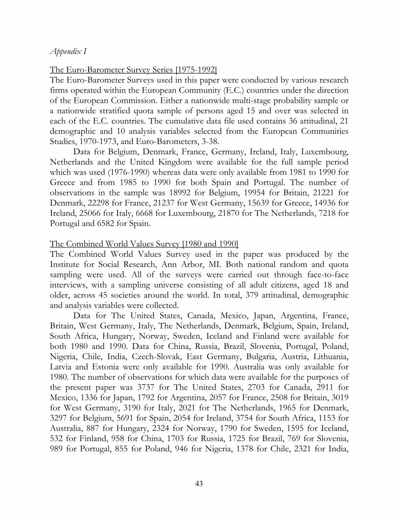
Appendix I The Euro-Barometer Survey Series [1975-1992] The Euro-Barometer Surveys used in this paper were conducted by various research firms operated within the European Community (E.C.) countries under the direction of the European Commission. Either a nationwide multi-stage probability sample or a nationwide stratified quota sample of persons aged 15 and over was selected in each of the E.C. countries. The cumulative data file used contains 36 attitudinal, 21 demographic and 10 analysis variables selected from the European Communities Studies, 1970-1973, and Euro-Barometers, 3-38.

Data for Belgium, Denmark, France, Germany, Ireland, Italy, Luxembourg, Netherlands and the United Kingdom were available for the full sample period which was used (1976-1990) whereas data were only available from 1981 to 1990 for Greece and from 1985 to 1990 for both Spain and Portugal. The number of observations in the sample was 18992 for Belgium, 19954 for Britain, 21221 for Denmark, 22298 for France, 21237 for West Germany, 15639 for Greece, 14936 for Ireland, 25066 for Italy, 6668 for Luxembourg, 21870 for The Netherlands, 7218 for Portugal and 6582 for Spain. The Combined World Values Survey [1980 and 1990] The Combined World Values Survey used in the paper was produced by the Institute for Social Research, Ann Arbor, MI. Both national random and quota sampling were used. All of the surveys were carried out through face-to-face interviews, with a sampling universe consisting of all adult citizens, aged 18 and older, across 45 societies around the world. In total, 379 attitudinal, demographic and analysis variables were collected. Data for The United States, Canada, Mexico, Japan, Argentina, France, Britain, West Germany, Italy, The Netherlands, Denmark, Belgium, Spain, Ireland, South Africa, Hungary, Norway, Sweden, Iceland and Finland were available for both 1980 and 1990. Data for China, Russia, Brazil, Slovenia, Portugal, Poland, Nigeria, Chile, India, Czech-Slovak, East Germany, Bulgaria, Austria, Lithuania, Latvia and Estonia were only available for 1990. Australia was only available for 1980. The number of observations for which data were available for the purposes of the present paper was 3737 for The United States, 2703 for Canada, 2911 for Mexico, 1336 for Japan, 1792 for Argentina, 2057 for France, 2508 for Britain, 3019 for West Germany, 3190 for Italy, 2021 for The Netherlands, 1965 for Denmark, 3297 for Belgium, 5691 for Spain, 2054 for Ireland, 3754 for South Africa, 1153 for Australia, 887 for Hungary, 2324 for Norway, 1790 for Sweden, 1595 for Iceland, 532 for Finland, 958 for China, 1703 for Russia, 1725 for Brazil, 769 for Slovenia, 989 for Portugal, 855 for Poland, 946 for Nigeria, 1378 for Chile, 2321 for India,

43

1391 for Czech-Slovak, 1280 for East Germany, 928 for Bulgaria, 1288 for Austria, 932 for Lithuania, 765 for Latvia and 890 for Estonia.

44

Appendix II The Microeconometric Determinants of the Desire for Revolution (Logit Regressions): 1976-90.

Dep Var: Revolution Desired?

U.K.

Italy

Germany

Belgium

Unemployed

0.373

(0.122)

0.287

(0.106)

-0.176

(0.211)

0.247

(0.108) Self employed

0.150

(0.124)

0.164

(0.075)

0.063

(0.173)

0.110

(0.110) Male

0.115

(0.071)

0.403

(0.059)

0.278

(0.096)

0.430

(0.071) Age

-0.009

(0.012)

-0.015

(0.011)

-6.7e-4 (0.016)

-0.038

(0.012) Age Squared

-7.7e-5

(1.3e-4)

-3.7e-5

(1.2e-4)

1.9e-5

(1.7e-4)

2.9e-4

(1.3e-4) Education to age: 15-18 years

-0.279

(0.096)

0.043

(0.073)

-0.210

(0.105)

-0.058

(0.079) ≥ 19 years

-0.530

(0.133)

0.090

(0.073)

-0.143

(0.139)

-0.291

(0.096) Marital Status: Married

-0.243

(0.094)

-0.204

(0.076)

-0.416

(0.122)

-0.041

(0.093) Divorced

-0.016

(0.163)

0.794

(0.260)

-0.044

(0.192)

0.467

(0.177) Separated

0.184

(0.216)

0.696

(0.193)

-0.066

(0.400)

0.373

(0.185) Widowed

-0.287

(0.155)

-0.346

(0.152)

-0.480

(0.194)

0.038

(0.164) No. of children ≥ 8 & 15 yrs: 1

0.127

(0.089)

-0.082

(0.067)

-0.039

(0.133)

0.078

(0.081) 2

0.238

(0.100)

-0.154

(0.100)

0.111

(0.168)

0.095

(0.112) 3

-0.135

(0.173)

0.224

(0.169)

0.324

(0.274)

0.241

(0.160) Income Quartiles: Second

-0.231

(0.092)

-0.166

(0.071)

-0.292

(0.111)

-0.162

(0.087) Third

-0.415

(0.098)

-0.282

(0.075)

-0.601

(0.122)

-0.311

(0.092) Fourth (highest)

-0.764

(0.109)

-0.301

(0.079)

-0.866

(0.133)

-0.447

(0.101) Retired

-0.040

(0.134)

-0.107

(0.118)

-0.634

(0.185)

-0.393

(0.138) School

0.275

(0.174)

0.113

(0.104)

0.060

(0.168)

0.054

(0.135) At home

0.022

(0.095)

-0.099

(0.095)

0.006

(0.135)

0.035

(0.105) Obs.

19,954

25,066

21,237

18,992

Notes: All regressions include region and year dummies from 1976 to 1990. For the U.K., Italy, Germany and Spain, Log-likelihood=-4474, -6325, -2715 and -4574, respectively, and Chi2(46)= 299, Chi2(38)=534, Chi2(44)=208 and Chi2(44)=343, respectively. Standard errors in parentheses.

Appendix III

P ro p o r t io nw h o

D es ireR ev o lu t io n

B e lg iu mY E A R

7 6 7 7 7 8 7 9 8 0 8 1 8 2 8 3 8 4 8 5 8 6 8 7 8 8 8 9 9 0

0

.0 2

.0 4

.0 6

.0 8

.1

.1 2

.1 4

P ro p o r t io nw h o

D es ireR ev o lu t io n

F ra n c eY E A R

7 6 7 7 7 8 7 9 8 0 8 1 8 2 8 3 8 4 8 5 8 6 8 7 8 8 8 9 9 0

0

.0 2

.0 4

.0 6

.0 8

.1

.1 2

.1 4

P ro p o rt io nw h o

D e s ireR e vo lu t io n

G e rm a n y Y E A R

7 6 7 7 7 8 7 9 8 0 8 1 8 2 8 3 8 4 8 5 8 6 8 7 8 8 8 9 9 00

.0 2

.0 4

.0 6

.0 8

.1

.1 2

.1 4

P ro po rtionw ho

D es ireR evo lu tion

D e n m a rkY E A R

76 77 78 7 9 80 81 82 8 3 84 85 86 8 7 88 89 90

0

.0 2

.0 4

.0 6

.0 8

.1

.1 2

.1 4

P ro p o r t io nw h o

D es ireR evo lu tio n

Ire la n dY E A R

7 6 7 7 7 8 7 9 8 0 8 1 8 2 8 3 8 4 8 5 8 6 8 7 8 8 8 9 9 0

0

.0 2

.0 4

.0 6

.0 8

.1

.1 2

.1 4

P ro p o rt io nw h o

D es ireR evo lu t io n

I ta lyY E A R

7 6 7 7 7 8 7 9 8 0 8 1 8 2 8 3 8 4 8 5 8 6 8 7 8 8 8 9 9 0

0

.0 2

.0 4

.0 6

.0 8

.1

.1 2

.1 4

P rop o rt io nw h o

D es ireR evo lu t io n

T he N e th e r la n d sY E A R

7 6 7 7 78 79 8 0 8 1 8 2 83 8 4 8 5 8 6 87 8 8 8 9 9 0

0

.0 2

.0 4

.0 6

.0 8

.1

.1 2

.1 4

P ropo rtionw ho

D es ireR evo lu tion

S p a inY E A R

76 77 78 79 80 81 82 83 84 85 86 87 88 89 90

0

.02

.04

.06

.08

.1

.12

.14

Proportionwho

DesireRevolu tion

U n ited K ingdomYEAR

76 77 78 79 80 81 82 83 84 85 86 87 88 89 90

0

.02

.04

.06

.08

.1

.12

.14

P ro p o rt io nw h o

D es ireR ev o lu t io n

G re e c e Y E A R7 6 7 7 7 8 7 9 8 0 8 1 8 2 8 3 8 4 8 5 8 6 8 7 8 8 8 9 9 0

0

.0 2

.0 4

.0 6

.0 8

.1

.1 2

.1 4

LuxembourgYEAR

76 77 78 79 80 81 82 83 84 85 86 87 88 89 90

0

.02

.04

.06

.08

Proportionwho

DesireRevolution Proportion

whoDesire

Revolution

PortugalYEAR

76 77 78 79 80 81 82 83 84 85 86 87 88 89 90

0

.02

.04

.06

.08

.1

.12

.14

47

Appendix IV Data Definitions Countries: Belgium, Britain, Denmark, France, Germany, Greece, Ireland, Italy, Luxembourg, The Netherlands, Portugal and Spain. The base category for the cumulative regression in Table D is France. REVOLUTIONARY SUPPORT: The coefficients on the year dummies from an Ordinary Least Squares regression of whether or not a respondent answers that “The entire way our society is organised must be radically changed by revolutionary action”, controlling for personal characteristics, for each country. NET INCOME: Average household current receipts per capita, after deducting direct taxes (=income taxes plus employee social security contributions), at 1985 price levels and exchange rates (in U.S. dollars), from the CEP-OECD data set [1950-1992]. INCOME INEQUALITY: The Gini coefficient from the Deininger and Squire (1996) ‘high quality’ data set. Missing years were linearly interpolated, which includes 1976-78 and 1980-83 for France; 1979-80 and 1982 for Germany; 1981-86 for Ireland; 1985, 1988 and 1990 for Italy; 1976, 1978, 1980 and 1984 for The Netherlands; 1980-84 and 1986-87 for Belgium; 1977-80, 1982-86 and 1988-90 for Denmark; 1985-87 for Greece; and 1985-89 for Portugal. No interpolated years were used for Britain, Luxembourg or Spain. MILITARY: Total military expenditures divided by GDP, from the Statistical Abstract of the United States and World Military Expenditures and Arms Transfers. OIL: An index of the country-specific price of oil, calculated as the price of oil in the local currency, divided by each nation’s GDP deflator and standardized to equal 1 across all nations in 1975. The oil price is taken from The Statistical Abstract of the United States (various issues). Exchange rate and GDP deflator data are from the CEP-OECD data set [1950-1992]. RIGHT WING: Index of left/right political party strength, defined as the sum of the number of votes received by each party participating in cabinet expressed as a percentage of total votes received by all parties with cabinet representation, multiplied by a left/right political scale constructed by political scientists. Votes are from Mackie and Rose’s (1982), The International Almanac of Electoral History, cabinet composition is from The Europa Yearbook (1969-1989 editions), and the left/right scale is from Castles and Mair (1984). OPENNESS: Imports plus exports, all divided by GDP, from CEP-OECD [1950-1992]. UNEMPLOYMENT: The unemployment rate, from CEP-OECD data set [1950-1992]. INFLATION RATE: Rate of change in the GDP deflator, from CEP-OECD [1950-1992].