what is your farm worth? - australian dairy conference is your farm worth? liesl malcolm –pitcher...

1

What is Your Farm Worth?Liesl Malcolm – Pitcher Partners

• Senior Manager in the Corporate Finance division of Pitcher Partners,

specialising in the valuation of all types of businesses, shares and

other equity instruments.

• Chartered Accountant and also an accredited Senior Appraiser with

the American Society of Appraisers.

• Discuss the valuation principles, how they apply to your business and

the key drivers in determining what your farm is worth.

• In particular we are going to discuss the discounted cash flow

approach.

• Ways in which you can increase the value of your farm.

Introduction

2

Enterprise/Business Value or Equity Value?

What is Being Valued?

3

Enterprise

/ Business

Value

Net Debt

& Surplus

Assets

Equity

Value

=

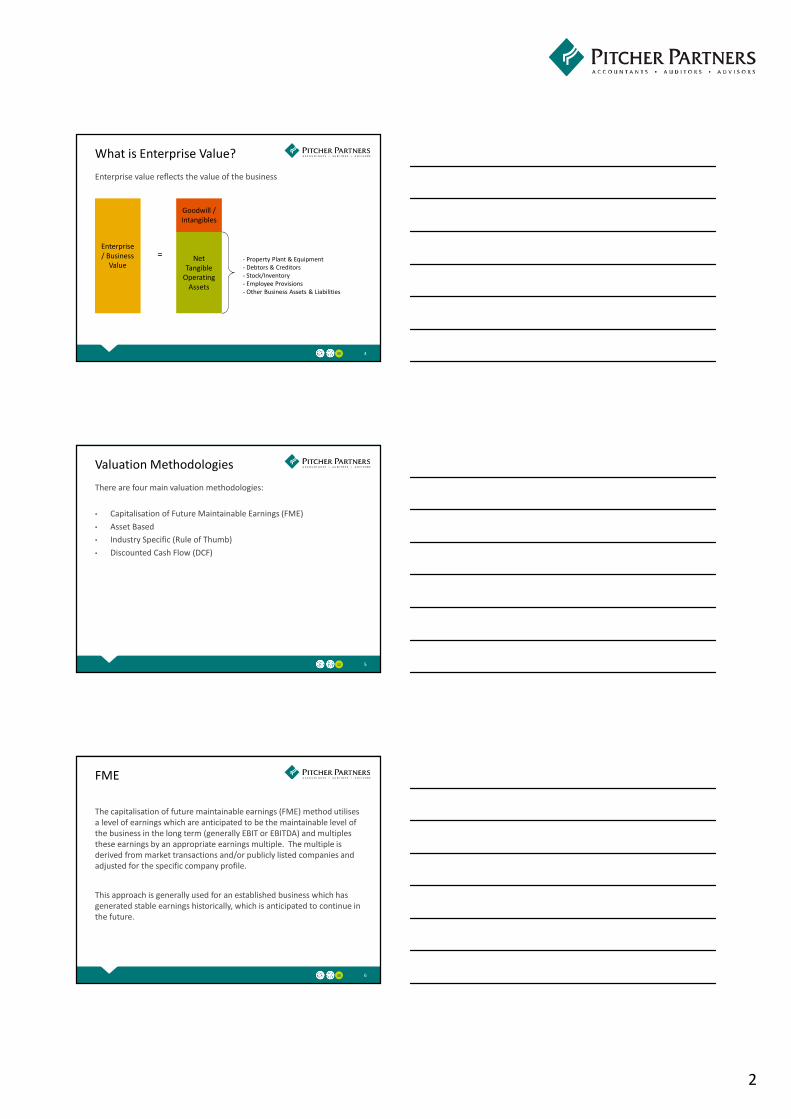
2

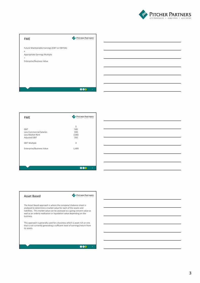
Enterprise value reflects the value of the business

What is Enterprise Value?

4

- Property Plant & Equipment

- Debtors & Creditors

- Stock/Inventory

- Employee Provisions

- Other Business Assets & Liabilities

Goodwill /

Intangibles

Net

Tangible

Operating

Assets

Enterprise

/ Business

Value

=

There are four main valuation methodologies:

• Capitalisation of Future Maintainable Earnings (FME)

• Asset Based

• Industry Specific (Rule of Thumb)

• Discounted Cash Flow (DCF)

Valuation Methodologies

5

The capitalisation of future maintainable earnings (FME) method utilises

a level of earnings which are anticipated to be the maintainable level of

the business in the long term (generally EBIT or EBITDA) and multiples

these earnings by an appropriate earnings multiple. The multiple is

derived from market transactions and/or publicly listed companies and

adjusted for the specific company profile.

This approach is generally used for an established business which has

generated stable earnings historically, which is anticipated to continue in

the future.

FME

6

3

Future Maintainable Earnings (EBIT or EBITDA)

x

Appropriate Earnings Multiple

=

Enterprise/Business Value

FME

7

FME

8

EBIT

Less Commercial Salaries

Less Market Rent

Adjusted EBIT

EBIT Multiple


$

500

(50)

(100)

350

4

1,400

The Asset Based approach is where the company’s balance sheet is

analysed to determine a market value for each of the assets and

liabilities. This market value can be assessed as a going concern value as

well as an orderly realisation or liquidation value depending on the

business.

This approach is generally used for a business which is asset rich or one

that is not currently generating a sufficient level of earnings/return from

its assets.

Asset Based

9

4

Market Value of Assets

-

Market Value of Liabilities

-

Costs of recovery (if applicable)

=

Equity Value

Asset Based

10

Asset Based

11

Net Book

Value

Adjustments Orderly

Realisation

$'000 $'000 $'000

Assets

Cash at Bank 171 - 171

Debtors 48 (5) 43

Inventory 96 (10) 86

Investments 253 (13) 240

Land and Buildings 4,930 (99) 4,831

Equipment 281 (28) 253

Intangibles 285 (285) -

Total Assets 6,064 (440) 5,624

Liabilities

Payables (324) - (324)

Employee Provisions (75) - (75)

Loans (1,500) - (1,500)

Total Liabilities (1,899) - (1,899)

Net Assets 4,165 3,725

Costs of Recovery (150)

Equity Value 4,165 3,575

An industry specific methodology uses some available industry measure

such as a revenue multiple or earnings multiple to apply to the business.

This methodology is not appropriate to use as a primary methodology

and is generally only used to cross check one of the other

methodologies.

Industry Specific

12

5

Revenue or other KPI measure

x

Industry multiple

=

Goodwill or Enterprise/Business Value

Industry Specific

13

$2 million revenue from recurring accounting fees

X

0.6 to 0.8 industry multiple

=

$1.2 million to $1.6 million goodwill

Industry Specific

14

The discounted cash flow (DCF) methodology has regard to the expected

future economic benefits discounted to present value. It uses the

forecast cash flows projected by the business in the short term, a

perpetuity or terminal value and an appropriate discount rate having

regard to market and company specific factors.

The DCF is most appropriate for a business with volatile earnings, a

growing or new business, or a changing business.

DCF

15

6

Future ungeared cash flows

Discounted using a discount rate (WACC)

=


DCF

16

The ungeared post tax cash flows utilised in a DCF are as follows:

Earnings before interest, tax, depreciation & amortisation (EBITDA)

-

Capital Expenditure

+/-

Decrease/increase in working capital

-

Tax (on EBIT)

=

Ungeared post tax cash flows

Cash Flows

17

Need to ensure that your cash flows reflect the following:

• adjustments for market rent

• if the land and buildings is owned by the business and is valued

separately, which is generally the case, then a market rental needs to

be included to avoid the double counting of the property

• adjustments for market salaries for all employees including

management and owners

• add backs of any non business expenditure

• capital expenditure requirements which are supportable

• tax payments reflect actual cash taxes paid

• working capital requirements of the business

Cash Flows

18

7

The cash flows are generally presented on an ungeared basis, so all

funding requirements are removed such as interest income and interest

expense.

The value of the business only is derived initially so as to determine the

value excluding the specific funding arrangements of the owner.

Any surplus cash and borrowings is valued separately when determining

the equity value of the business.

Cash Flows

19

• Scenario 1 – Assume 100% ownership of the business and farm

• Scenario 2 – As above, but assuming the farm is leased

• Scenario 3 – The same as scenario 2, expect that an employee has

purchased an equity stake in the business via a herd lease for a

number of cows.

5 Year Cash Flows – Farm

Scenarios

20

Cash Flows – Scenario 1

21

Year 1 Year 2 Year 3 Year 4 Year 5

Net Revenue 1,000 1,030 981 1,020 1,061

Other Expenses (830) (852) (803) (833) (866)

Less Notional Market Rent (80) (85) (90) (95) (100)

EBITDA 90 93 88 92 95

EBITDA Margin 9% 9% 9% 9% 9%

EBITDA 90 93 88 92 95

less Capital Expenditure (25) (40) (25) (25) (25)

less Working Capital Movements (5) (5) (5) (5) (5)

less Tax (21) (22) (21) (21) (22)

Free Cash Flow 39 26 37 41 43

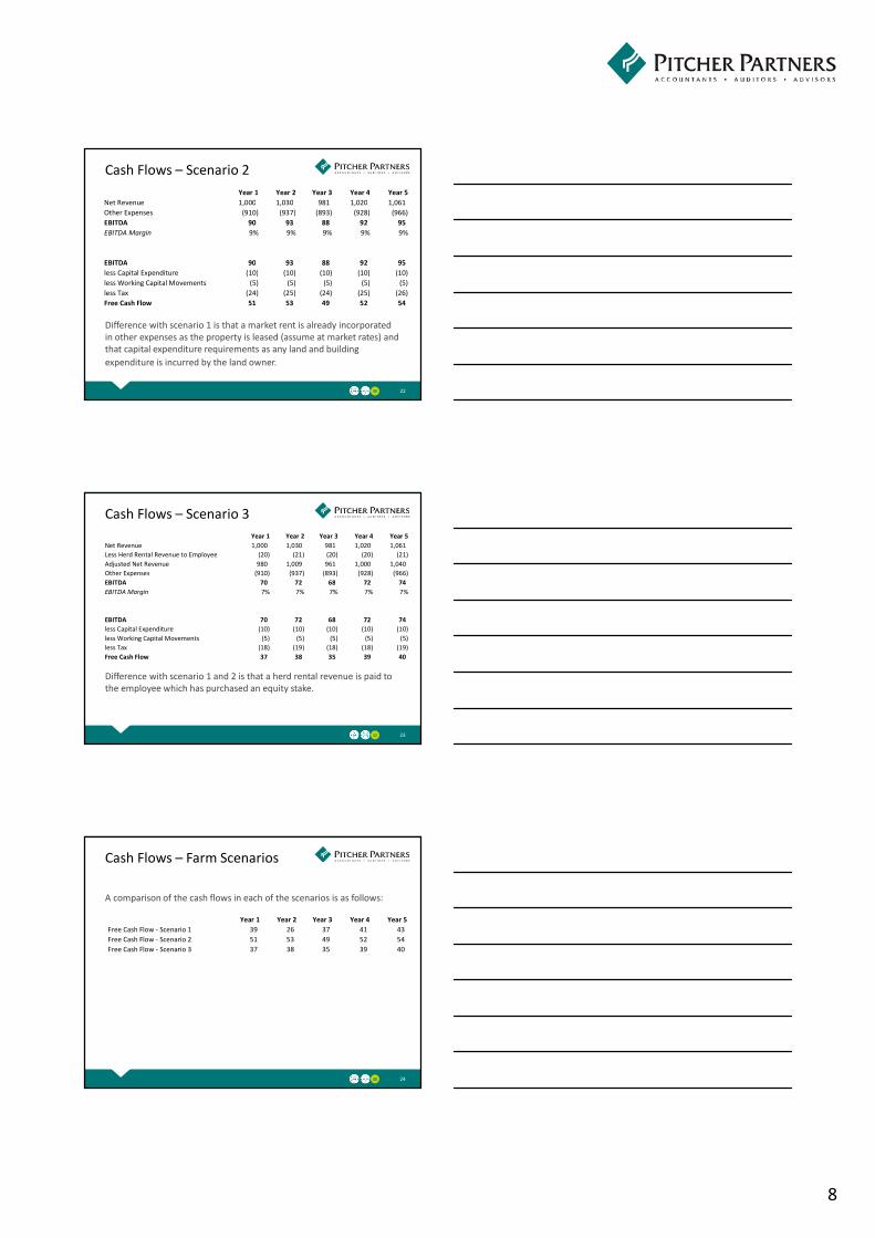
8

Difference with scenario 1 is that a market rent is already incorporated

in other expenses as the property is leased (assume at market rates) and

that capital expenditure requirements as any land and building

expenditure is incurred by the land owner.


22


Net Revenue 1,000 1,030 981 1,020 1,061

Other Expenses (910) (937) (893) (928) (966)

EBITDA 90 93 88 92 95


EBITDA 90 93 88 92 95



less Tax (24) (25) (24) (25) (26)


Difference with scenario 1 and 2 is that a herd rental revenue is paid to

the employee which has purchased an equity stake.


23


Net Revenue 1,000 1,030 981 1,020 1,061

Less Herd Rental Revenue to Employee (20) (21) (20) (20) (21)

Adjusted Net Revenue 980 1,009 961 1,000 1,040

Other Expenses (910) (937) (893) (928) (966)

EBITDA 70 72 68 72 74


EBITDA 70 72 68 72 74



less Tax (18) (19) (18) (18) (19)


A comparison of the cash flows in each of the scenarios is as follows:

Cash Flows – Farm Scenarios

24


Free Cash Flow - Scenario 1 39 26 37 41 43



9

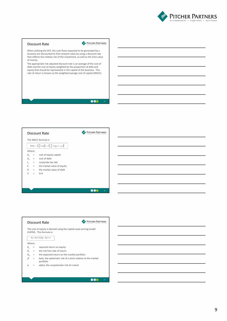
When utilising the DCF, the cash flows expected to be generated by a

business are discounted to their present value by using a discount rate

that reflects the relative risk of the investment, as well as the time value

of money.

The appropriate risk adjusted discount rate is an average of the cost of

debt and the cost of equity weighted by the proportion of debt and

equity that should be represented in the capital of the business. This

rate of return is known as the weighted average cost of capital (WACC).

Discount Rate

25

The WACC formula is:

Where:

Ke = cost of equity capital

Kd = cost of debt

tc = corporate tax rate

E = the market value of equity

D = the market value of debt

V = D+E

Discount Rate

26

�� = ( �

�× Ke) + (

�

� × Kd 1 − tc )

The cost of equity is derived using the capital asset pricing model

(CAPM). This formula is:

Where:

Ke = required return on equity

Rf = the risk free rate of return

Rm = the expected return on the market portfolio

β = beta, the systematic risk of a stock relative to the market

portfolio

α = alpha, the unsystematic risk of a stock

Discount Rate

27

Ke = Rf + � (Rm − Rf ) + �

10

The risk free rate on equity is derived with reference to the long term

government bond rate, currently this is approximately 3.5%.

The accepted market risk premium in Australia is between 5% and 7%.

The beta is derived from a list of comparable listed companies. The beta

of a stock is determined by the characteristics of the company and is

generally based on three factors:

• the nature of revenue and the extent to which it is cyclical;

• operating leverage; and

• financial leverage

A beta of 1 reflects a market beta, less than 1 means is generally less

risky than that of the market and greater than 1 means it moves

disproportionately to the market.

Cost of Equity

28

The unsystematic risk factor incorporates additional risks to the

company being valued as compared to the market such as small

company risk and diversification.

This component is where the risks specific to each business being valued

are taken into consideration.

The more risky a business is the higher the unsystematic risk factor and

the discount rate.

The higher the discount rate, the lower the value of the business.

Cost of Equity

29

The current cost of debt for dairy farms ranges from 6% to 9%. The rate

applied should be that specific to the dairy farm being valued, so

whatever the available optimum borrowing rate would be to the

farmer/operator.

Cost of Debt

30

11

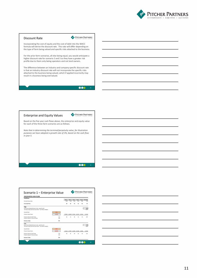
Incorporating the cost of equity and the cost of debt into the WACC

formula will derive the discount rate. This rate will differ depending on

the type of farm being valued and specific risks attached to the business.

For the prior farm scenarios, all else being equal, you would anticipate a

higher discount rate for scenario 2 and 3 as they have a greater risk

profile due to them only being operators and not land owners.

The difference between an industry and company specific discount rate

is that an industry discount rate will not incorporate the specific risks

attached to the business being valued, which if applied incorrectly may

result in a business being overvalued.

Discount Rate

31

Based on the five year cash flows above, the enterprise and equity value

for each of the three farm scenarios are as follows.

Note that in determining the terminal/perpetuity value, for illustration

purposes we have adopted a growth rate of 3%, based on the cash flow

in year 5.

Enterprise and Equity Values

32

Scenario 1 – Enterprise Value

33

DISCOUNTED CASH FLOW

CashflowsYear 1 Year 2 Year 3 Year 4 Year 5 Terminal

Periods Discounting 0.50 1.50 2.50 3.50 4.50 4.50

Free Cash Flow 39 26 37 41 43 45

HighCash flow multiple (discount rate - growth rate) 8.3

Terminal Value (terminal cash flow * cash flow multiple) $373

Growth Rate 3.0%

Present Value Factor 15.00% 0.9325 0.8109 0.7051 0.6131 0.5332 0.5332

Present Value of Cash Flows 132 36 21 26 25 23 199

Present Value of Terminal Value 199

Business Value 331

LowCash flow multiple (discount rate - growth rate) 5.9


Growth Rate 3.0%




Business Value 235

12

Scenario 1 – Equity Value

34

Low High

$'000 $'000

Enterprise Value 235 331

Add Land and Buildings (market value) 5,000 5,000

Less Debt (4,000) (4,000)

Equity Value 1,235 1,331

To determine the equity value, need to consider any surplus assets and

debt items. In this scenario, the operator also is the land owner, the

surplus asset will be the land and buildings (as a market rent has been

charged in the cash flows) and the debt will be the loan attached to it.


35




Free Cash Flow 51 53 49 52 54 56



Growth Rate 3.0%




Business Value 377



Growth Rate 3.0%




Business Value 284


36


debt items. In this scenario, the operator does not own the land and

buildings and has no surplus cash. It does however have a small amount

of bank debt.

Low High

$'000 $'000


Add Land and Buildings (market value) - -

Less Debt (20) (20)

Equity Value 264 357

13


37




Free Cash Flow 37 38 36 38 40 41



Growth Rate 3.0%




Business Value 277



Growth Rate 3.0%




Business Value 219


38


debt items. In this scenario, the operator does not own the land and

buildings but has some surplus cash from the employee purchase of a

herd. It does also have a small amount of bank debt.

Low High

$'000 $'000


Add Surplus Cash (from Sale of Herd) 120 120

Add Land and Buildings (market value) - -

Less Debt (20) (20)

Equity Value 319 377

Comparison – Enterprise and

Equity Values

39

Enterprise Values

Scenario 1 235 331

Scenario 2 284 377

Scenario 3 219 277

Equity Values

Scenario 1 1,235 1,331

Scenario 2 264 357

Scenario 3 319 377

14

The number one and easiest way to increase the value of your farm is to

increase your earnings and profitability. The greater the cash flows,

providing they are realistic and supportable, the greater the value of

your farm.

However, there are also other ways in which you can increase the value

as they reduce the risk of the business. These include:

• stable workforce with long term employees

• succession plans for key staff to reduce the reliance on these key

people

• strong management team

• strong relationships with customers (and suppliers)

• building new relationships with new customers

How to Increase the Value of

your Farm

40

• development of a business plan setting the short and long term

strategy for the business

• negotiating favourable agreements with key stakeholders, for

example a long term lease with the owner of the farm/property

• monitoring the performance of competitors and identifying ways in

which the farm could improve

• corporatise the farm as much as possible, document all policies and

procedures, OH&S plans, prepare detailed financial statements,

prepare forecasts/budgets, undertake industry research, training

manuals, etc.

How to Increase the Value of

your Farm

41

• Enterprise value is the value of the business whereas Equity Value is

the return to the equity holders after repayment of all debt.

• There are three main methodologies to value a business, FME,

Assets, Industry and DCF.

• FME is best for a stable business.

• Assets based is appropriate for an asset rich business.

• Industry methodology is generally only used as a cross check.

• DCF is best for a growing, volatile or changing business.

• Discount rate is a rate which reflects the relative risk of the

investment, as well as the time value of money. The greater the

discount rate the lower the value.

Overview

42

15

• Incorporated in the discount rate is an unsystematic risk factor which

relates to the specific risks of the business compared with the

market.

• Difference between an industry and company discount rate is that

the industry discount rate will not incorporate the specific risks of a

business.

• There are a number of ways in which you can increase the value of

your farm, these include improving the earnings and profitability of

your business, corporatising the farm, strong management and

workforce and key relationships with stakeholders.

Overview

43

Go ahead. Don’t hesitate.Q&A

44

Questions & Answers

Thank youFor your attention

45

Thank you!

16

46

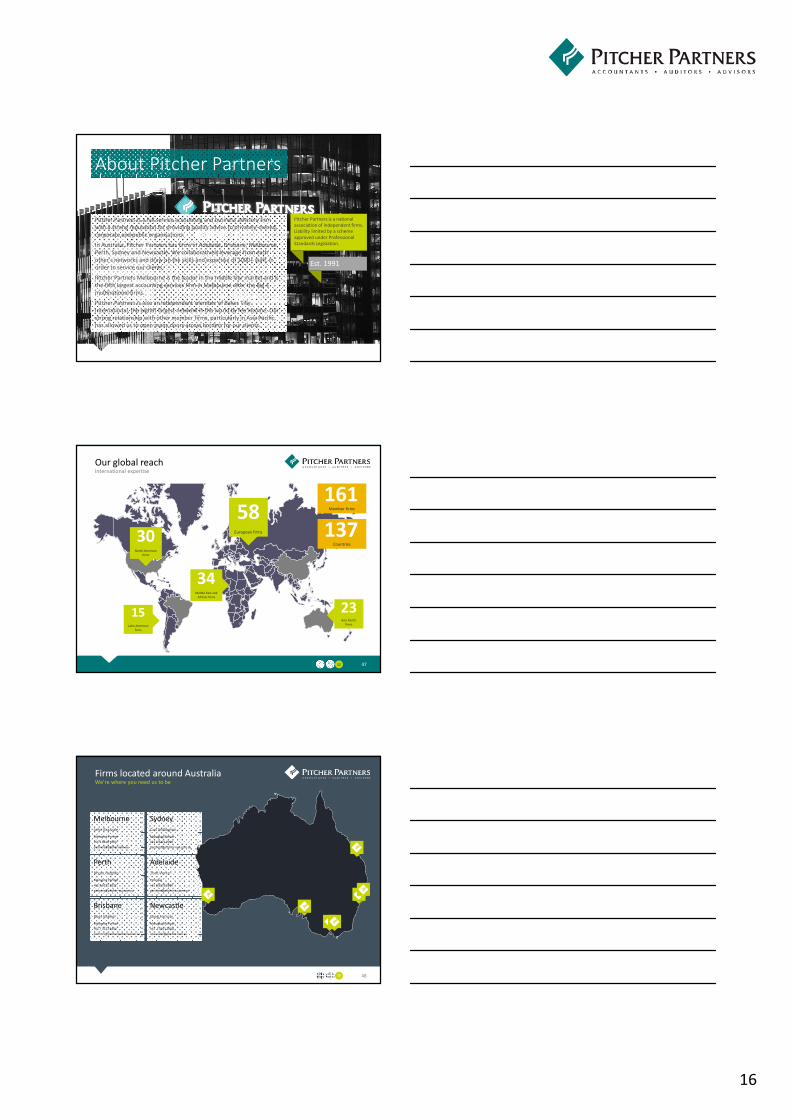
Pitcher Partners is a full service accounting and business advisory firm

with a strong reputation for providing quality advice to privately-owned,

corporate and public organisations.

In Australia, Pitcher Partners has firms in Adelaide, Brisbane, Melbourne,

Perth, Sydney and Newcastle. We collaboratively leverage from each

other’s networks and draw on the skills and expertise of 1000+ staff, in

order to service our clients.

Pitcher Partners Melbourne is the leader in the middle-tier market and is

the fifth largest accounting services firm in Melbourne after the Big 4

multinational firms.

Pitcher Partners is also an independent member of Baker Tilly

International, the eighth largest network in the world by fee income. Our

strong relationship with other member firms, particularly in Asia Pacific,

has allowed us to open many doors across borders for our clients.

Pitcher Partners is a national

association of independent firms.

Liability limited by a scheme

approved under Professional

Standards Legislation.

Est. 1991

About Pitcher Partners

Our global reachInternational expertise

47

North American

firms

30

Middle East and

African firms

34

European firms

58

Latin American

firms

15Asia Pacific

firms

23

Member firms

161

Countries

137

48

Firms located around AustraliaWe’re where you need us to be

Melbourne

John Brazzale

Managing Partner

+61 3 8610 5000

[email protected]

Sydney

Carl Millington

Managing Partner

+61 2 9221 2099

[email protected]

Perth

Bryan Hughes

Managing Partner

+61 8 9322 2022

[email protected]

Adelaide

Tom Verco

Principal

+61 8 8179 2800

[email protected]

Brisbane

Ross Walker

Managing Partner

+61 7 3222 8444

[email protected]

Newcastle

Greg Farrow

Managing Partner

+61 2 4911 2000

[email protected]

what is your farm worth? - australian dairy conference is your farm worth? liesl malcolm –pitcher...

Documents