Department of Economics and Finance

Working Paper No. 10-01

http://www.brunel.ac.uk/about/acad/sss/depts/economics

Econ

omic

s an

d Fi

nanc

e W

orki

ng P

aper

Ser

ies

Ahmed A. Alzahrani and Andros Gregoriou

What Happens Around Earning Announcements? An Investigation of Information Asymmetry and Trading Activity in the Saudi Market

March 2010

1

What Happens Around Earning Announcements? An Investigation of Information Asymmetry and

Trading Activity in the Saudi Market.

Ahmed A. Alzahrani*

Department of Economics and Finance, Brunel University

Andros Gregoriou

Norwich Business School, University of East Anglia

Abstract:

This paper examines stock returns and trading activities around earnings announcements for

listed companies in the Saudi stock market (SSM). Specifically, we examine the levels of

stock liquidity, trading activity, volatility, bid-ask spread, asymmetric information and

investor trading behaviour around earnings announcements for all firms in the market for the

period 2002-2009. Abnormal price and volume reactions around earnings announcements

suggest that these announcements produce highly informative contents. The magnitude of the

cumulative abnormal returns around earnings announcement is induced by trading activity in

the two weeks before the release date. We also show evidence of an increased adverse

selection cost around earnings announcement, which is then gradually reduced in the post-

announcement period, indicating that earnings announcements reduce uncertainty in the

market. We also examine trading behaviour among small and large investors in the market

through constructing order imbalance measures. In general, large investors are more

sophisticated and show higher informed trading before earnings announcements whereas

smaller investors show stronger reaction to news. Moreover, small investors show a buying

pattern which is consistent with times-series based earnings surprise. They are net-buyers for

good news and net-sellers for bad news portfolios.

Corresponding author: zahraniaa@ipa.edu.sa

2

1 Introduction

Our paper is motivated by many factors: first, we investigate the Saudi stock market

(hereafter, SSM) to provide out-of-sample evidence regarding the on-going debate about

Post-Earnings Announcements Drift (PEAD) and the way in which it can be explained,

because the nature of this anomaly is not well understood. Second, the SSM is dominated by

individual investors, 90% of its total trading, which provides an ideal setting for studying

how investors react to informational events. Third, the SSM has unique institutional

characteristics which make it suitable to test for these characteristics on stock returns and

trading activities. For instance, it allows no short selling nor derivatives trading. Moreover

few analysts follow the market and reports are scarce and not regularly published, which

makes it hard to anticipate earnings and news in the market. Finally, the SSM is an order-

driven market; thus, analysing traders‟ placement strategies around earnings announcements

provides an insight which is applicable to other order-driven markets.

All these factors motivate us to study how information content affects trading behaviour

around earnings announcements. It is of great value to both academics and practitioners to

study the effect of these unique aspects on stock trading and return behaviour.

The paper is organized as following. Section discusses the literature review. Sections 3 & 4

illustrate the data and methodology used to implement the event study. Section 5 documents

the event study restuls. Section 6 empirically examines the magnitude of abnormal returns

and information asymmetry around earnings announcments. Finally, Section 7 summarizes

and concludes.

2 Literature review

For over 40 years, researchers have consistently documented the phenomena in stock markets

where stock prices tend to drift in the direction of the earnings surprise following earnings

announcements; this phenomenon is called Post-Earnings Announcements Drift (PEAD). In

this study, we explore the trading activities around earnings announcements with the aim of

3

examining how investors and the market in aggregate level behave around earnings

announcements. This behaviour is reflected in trading volume, volatility, bid/ask spread,

abnormal returns, order imbalance and other factors. A vast body of research has documented

the tendency of stock price returns to show a continuous drift after the release of earnings

announcement .The systematic increase in price returns around earnings announcements can

be observed in periods either before or after earnings announcements .Early event studies

even document that the information content of earnings announcement not only affects

returns, but other stock characteristics of trading, such as higher abnormal trading volume

surrounding announcements (Beaver, 1968).

Many researchers have confirmed the robustness of PEAD using different techniques and

different data (e.g., Bernard and Thomas, 1989;Ball, 1992). Findings of research on the

capital market suggest that earnings announcements contain information which is believed to

alter investors‟ opinion about the values of stocks, through the process of impounding

information into prices. This impounding of information into prices and trading activities

suggests the existence of privately informed traders and leakage of information

PEAD is typically explained by the magnitude of the earnings surprises or unexpected

component of the earnings. The higher the surprise (the difference between anticipated

earnings and actual earnings), the higher the drift found. In attempting to explain the drift,

many studies have distinguished between individual trading and institutional trading and

suggest that institutional trading is more sophisticated than individual trading. On this basis,

individual trading may be more closely related than institutional trading is to market

inefficiencies in general and PEAD in particular (see, for instance, Walther, 1997; Berkman

et al., 2009). However, recent research provides some evidence that even relatively more

sophisticated investors have difficulty in processing financial information which could delay

the price reaction to news (Callen et al., 2005).

Analysing trading activities around earnings announcements should provide us with a clearer

picture of the way in which different aspects of the market respond in general, not only the

stock returns. The persistent increase of stock returns can be induced by factors other than the

earnings surprise. Liquidity, level of information asymmetry, trading volume and order

imbalance can all have major effects on price drift.

4

Trading volume and volatility

In general, stock returns and trading volume tend to be positively correlated. Stocks tend to

rise on high volume and decline on low volume.1 Most of the theories explaining the volume-

return relationship emphasise the dispersion of beliefs among investors. Earnings

announcements provide an ideal environment to test the volume effect on returns, because

they are regular, exogenous, generate substantial volume and have almost fixed intervals

(Frazzini and Lamont, 2007).

Past empirical work shows that stock returns around earnings announcements are usually

associated with an increase in trading volume and volatility. Trading volume usually

increases in response to earnings announcements, due to the reduction of information

uncertainty among investors. In addition, as some researchers suggest, investors have

different levels of ability to process information and may interpret earnings news differently,

hence responding differently (Karpoff, 1986; and Kim and Verrecchia, 1994).

Other researchers have explained the relationship between volume and returns in the context

of noise traders. Higher trading volume indicates the presence of irrational or noise traders,

who push up prices (Baker and Stein, 2004). Other similar explanations have focused on the

“attention-grabbing hypothesis”, under which individual traders have limited attention and

rarely use short selling. If a stock attracts their attention, they are likely to buy it, regardless

of the nature of the news good or bad. This hypothesis predicts that stocks in the news have

both high volume and high net buying by individuals (Barber and Odean, 2008).

Frazzini and Lamont (2007) find that, around earnings announcements, stocks with high

volume have subsequently both high premiums and high imputed buying by individual

investors.

If new information is believed to either increase or decrease uncertainty in the market, then

we can safely assume that volatility will also change around earnings announcements. The

increase in return volatility and trading volume around earnings announcements compared

with non-announcement periods is well documented in the literature. However, the

relationship property between volatility in the post-announcement period and the content or

precision of the earnings announcement cannot be exactly defined.

1 See, among others, Karpoff‟s review of the subject (1987)

5

Acker (2002) links volatility with the content of the earnings announcement. If an

announcement is easy to interpret or contains good news, an increase in volatility is usually

observed on the day of the announcement, while bad news or difficult-to-interpret news has a

delayed price and volatility reaction until the following day.

Liquidity and information asymmetry

Hakansson (1977) shows that if investors differ in their information acquisition abilities or

resources, different patterns of information acquisition and processing emerge. In making

investment decisions, investors with low information processing skills or resources (small

investors) tend to rely on public information, whereas more sophisticated investors with

better information processing skills or resources rely on pre-disclosure information. Kim and

Verrecchia( 1991) suggest that since some investors are asymmetrically informed before the

anticipated announcement, they may respond to it differently.

Demsetz (1968) proposes the bid-ask spread as a measure of liquidity where the spread

reflects the adverse selection costs entailed by asymmetric information among investors.

Higher information asymmetry would increase the adverse selection cost and this is reflected

in a wider bid-ask spread. More recent papers have shown that adverse selection or

information asymmetry component represents a significant portion of the spread and that

increased adverse selection cost is the dominant factor affecting bid-ask spread around

earnings announcements. Kim and Verrecchia (1994) argue that, due to the different levels of

ability of market participants to process information, information asymmetry should not only

increase on the day before the announcement, but should also stay at a high level in the post-

announcement period, since some investors are better able to interpret news than other. Some

participants, for example, process the public information (earnings announcements) into

private information about a firm‟s performance and make better informed judgements.

Chiang and Venkalesh (1986) and Glosten and Harris, (1988) among many others, suggest

that spreads are negatively associated with trading volume and share price but positively

associated with return volatility. Affleck-Graves et al. (2002) find that, on the day of the

announcement, the adverse selection component of the spread increases. They also find that

component increases even before the announcement day and suggest that spread is used as a

proxy for both information asymmetry and market liquidity. Handa et al. (2003) argue that

6

spread serves also as a proxy of information asymmetry in an order-driven market, because it

is a function of adverse selection and also of difference in valuation among investors.

The inconclusive evidence of information asymmetry and liquidity behaviour around

earnings announcements has been explained by Krinsky and Lee (1996), who investigate the

spread components around earnings announcements and find an offsetting effect. While

other components decrease because of higher trading volume, adverse selection costs

increase because some traders have a superior capacity to estimate firm performance.

Because the SSM is an order-driven market, we also study the traders‟ order placement

strategies around the release of this accounting information by classifying traders into two

categories, large and small. The different analyses allow us to infer the effect of earnings

announcements on the level of information asymmetry and market liquidity among different

types of investor.

Since earnings announcements convey new information to the market as observed through a

reduction in information asymmetry, some investors will actively seek information in the pre-

disclosure period which will be reflected in the concentration of trading activities before the

earnings announcement. Trading activities can be examined by various groups of variables

(i.e., trading volume, bid/ask spread and number of buy and sell orders in the market). On the

basis of the earlier arguments, we expect quarterly earnings announcements in the SSM to

exhibit significant abnormal returns, higher abnormal trading volume, wider bid-ask spread

and more net buying by small traders. We also predict that the stock market reaction occurs

even before the day of the earnings announcement, for some investors will be actively

seeking information in this period and this will increase the information asymmetry before

the expected release date.

Like Lakhal (2008), we conjecture that, in an order-driven market such as the SSM, earnings

announcements are likely to narrow the subsequent bid-ask spread and to increase trading

volume around the day of the announcement, thus improving market liquidity and reducing

information asymmetry. We also anticipate that the spread increases before the

announcement is made, because liquidity traders widen the spread in order to compensate for

their potential losses from trading with informed traders.

7

3 Data

We use three sets of data:

1) Earnings announcements data which are recorded manually from the official stock

exchange bulletin (Tadawul) with their time and date stamped. We document 2,437 quarterly

earnings announcements covering the period between Q1 in 2002 and Q2 in 2009. After

removing announcements whose time or date cannot be verified or announcements

coinciding with those of other corporate events, we are left with 2170 earnings

announcements. For each observation, we document the date, earnings and nature of the news

as good or bad, compared either with the reaction of prices to the news on the announcement

day or to a seasonal ranking walk surprise measure. Ninety-five listed firms are included in

the sample, which each have at least six observations (earnings announcements). 2

2) Data regarding stock daily prices for all stocks and market index were provided by the

official stock exchange bulletin, Tadawul. It includes the following fields: Close, High, Low,

Volume, Value and Trades for the eight-year period of 2002-2009.

3) Intraday data for all trades stamped to the nearest minute for the same period with the

same field for the daily stock data. These data are extracted with a programming capability

which stores and processes all historical data. Current high frequency data providers in the

SSM provide data only for the last 25 days. These data were used for estimating the bid- ask

spread, calculating order imbalance, classifying traders into small and large, computing the

number of buyer and seller initiated trades and finally for computing intraday volatility.

All the listed companies in the SSM are required to publish their earnings in the

fortnight starting from the last day of the quarter, but the exact timing of announcements is

not known until they have been made public. At the end of each financial year,

announcements must be made in the first forty days from the end of each company‟s

financial year.

Our unique datasets allow us to precisely investigate trading activities around

earnings announcements in more detail, since intraday data has never been used in this

market.

2 The sample firms represent around 95% of the total market value , only newly-found firms which haven‟t

made operating earnings were excluded.

8

4 Methodology

We first use standard event study to capture the informativeness of earnings announcements

through estimating daily abnormal returns, trading activity measures, volatility and spread

over time.3 To compute abnormal return (AR) and cumulative abnormal return (CAR), we

consider the following two return generating models (i.e., models for „normal returns‟):

A) Market-adjusted return model

𝑨𝑹𝒊𝒕= 𝑹𝒊𝒕 − 𝑹𝒎𝒕 (1)

Where the abnormal return is the difference between the raw return 𝑅𝑖𝑡 and the market return

(TASI index) 𝑅𝑚𝑡 at time t,

B) Market model where returns are estimated using the following equation:

𝐄(𝐑𝐢𝐭

) = 𝛂𝐢 + 𝛃𝐢 (𝐑

𝐦𝐭) (2)

Then estimated returns are subtracted from the raw returns 𝑹𝒊𝒕 to formulate the abnormal

returns 𝑨𝑹𝒊𝒕 . If an earnings announcement occurs within trading hours, then the

announcement day is labelled day 0. If an announcement is made after the close of the day,

then day 0 is the next trading day. The abnormal return for a given day is computed as the

difference between the realised returns predicted from the market model and the raw

returns 𝑅𝑖𝑡 . Abnormal returns are then aggregated across two dimensions, across events or

firms (cross-section) and across a time interval [t1, t2]. Within the event window sample, the

cross-sectional averages of all stock returns and other measures are constructed for each day

and then a time series of cross-section averages is computed for the whole event window. To

construct a control sample, the time series for each stock [-100,-11] relative to the day of the

earnings announcement (day 0) is formed, to estimate the parameters. The time-series

averages of these cross-sectional measures are then calculated to arrive at a single number

which represents the control for comparison purposes for the measures of trading activity.

Cumulative Abnormal Returns (CARs) are then computed for various windows around the

event day. We define our event period to be various event windows [-10, +10], [-5, +5] and

[-1, +1], so as to fully capture the earnings announcements effects. We focus on stock returns

3 For reviews of the subject and event study econometrics, see MacKinlay (1997); Campbell et al. (1997);

Binder(1998); and Kothari and Warner (2007).

9

and trading activity during the 21-, 11- and 3-day event windows around earnings

announcements.

Measures of trading activities and information asymmetry

For trading activates, we assign our “normal period” for trading activities to be days [-30,-

11]. We then construct our measure of abnormal trading activity for each day in the event

window relative to our “normal” control period. We compare the behaviour pattern of each

variable around the earnings announcement to its “normal behaviour” estimated from the

non- announcement control period (benchmark period). For each variable chosen, the

abnormal measure is normalised and defined as:

𝑽𝒆𝒗𝒆𝒏𝒕 − 𝑽 𝒃𝒆𝒏𝒄𝒉𝒎𝒂𝒓𝒌

𝑽𝒂𝒓(𝑽 𝒃𝒆𝒏𝒄𝒉𝒎𝒂𝒓𝒌)

Where Vevent is the event period interval, 𝑉 𝑏𝑒𝑛𝑐 ℎ𝑚𝑎𝑟𝑘 is the mean value over the benchmark

period intervals [-30,-11] and 𝑉𝑎𝑟(𝑉 𝑏𝑒𝑛𝑐 ℎ𝑚𝑎𝑟𝑘 ) is the standard deviation over the control

period [-30,-11]. Because we are interested in observing the change in trading activity around

corporate events, we do not focus on the level of trading activity, but rather in recognising

unusual activity. The deviation from normal trading activity is measured through normalising

these trading activities.

We use various measures of trading activates which have been used in the literature to

capture the market behaviour before, during and after the earnings announcement day. We

consider three different measures of trading activity; trading volume (TV) in SAR, share

turnover (Turnover) which is computed as a percentage of the daily volume traded relative to

outstanding shares and the number of trades (NT), since these measures have been used

frequently to proxy for the level of trading activity. For the remaining variables, we define

each variable and document how it is computed below.

For the volatility measure we use the intraday high-low price range. For the liquidity and

information asymmetry, we use three measures: the bid-ask spread, order imbalance and

overnight indicator. We define each variable and document according to the way in which it

is computed.

10

Volatility (VOL) is measured as daily High and Low prices scaled by Low prices. The

market volatility is expected to increase around the date of the earnings announcement due to

the release of price-sensitive information. We compute our volatility measure similarly to

those of Bushee et al. (2003) which can be written as follows:

𝑽𝑶𝑳𝒊,𝒕 =

𝑷𝒊,𝒕𝑯 − 𝑷𝒊,𝒕

𝑳

𝑷𝒊,𝒕𝑳

(3)

where 𝑃𝑖,𝑡 denotes respectively the highest (H) and the lowest (L) prices for firm i and day t.

Bid-ask spreads are used as a proxy for both information asymmetry and liquidity. Spreads

are commonly considered a proxy for information asymmetry .The wider spreads reflect the

higher adverse selection cost, as suggested by many researchers (see, for example, Coller and

Yohn, 1997; Affleck-Graves et al., 2002). The order processing and inventory components

reflect the liquidity while the adverse selection component reflects the information

asymmetry. We follow Affleck-Graves et al. (2002), who suggest using the bid-ask spread as

proxy for both the liquidity and information asymmetry.

Since quote data are not directly available in the SSM, we estimate the spread using high

frequency data (with one-minute intervals). We make use of the covariance model of George

et al. (1991) which shows how the first-order auto-correlation in stock returns can be used to

estimate the bid-ask spread.

They estimate the informational asymmetry component of the bid-ask spread, ∅i,m = 1 −

πi,m which is that part of the spread that is derived from the information asymmetry of firm i

and time 𝑚 . George et al (1991) used daily prices, but we use intraday prices at one-minute

intervals; hence, we give the time period the subscription 𝑚. Furthermore, πi,m represents

that part of the spread which is not due to information asymmetry. The spread estimation

equation can be written as follows:

𝝅𝒊,𝒎 =𝟐 −𝒄𝒐𝒗 𝑹𝑫𝒊,𝒕 ,𝑹𝑫𝒊,𝒕−𝟏

𝑺𝒊,𝒅

(4)

11

where 𝑅𝐷𝑖,𝑡 = 𝑅𝐷𝑖𝑇𝑡 − 𝑅𝐷𝑖𝐿𝑡 is the difference between the intraday returns of the

transaction prices 𝑅𝐷𝑖𝑇𝑡 and bid prices 𝑅𝐷𝑖𝐿𝑡 (intraday Low prices) ,𝑅𝐷𝑖,𝑡−1 is the one-

minute lag of 𝑅𝐷𝑖,𝑡 , 𝑅𝐷𝑖𝑇𝑡 is the 1-minute intraday return of firm i using the transaction

prices of the time interval between t-1 and t, 𝑅𝐷𝑖𝐿𝑡 is the 1-minute intraday return of firm i

using bid prices computed between time t-1 and time t, 𝑆𝑖 ,𝑑 is the average of intraday bid-

ask spreads of all transactions recorded for firm i on day d and finally 𝑐𝑜𝑣 𝑅𝐷𝑖,𝑡 , 𝑅𝐷𝑖,𝑡−1 is

the serial covariance of 𝑅𝐷𝑖,𝑡 .4

The overnight indicator (ONI) of Gallo and Pacini (2000) is used to measure the

disagreement and dispersion of opinion among investors regarding the fundamental value of

a stock. ONI represents the surprise between the closing of one day and the opening of the

next day; we find this a good proxy for information asymmetry and arrival in the SSM.5 It is

calculated as follows:

𝑶𝑵𝑰𝒕 = 𝒍𝒐𝒈

𝑶𝒑𝒆𝒏𝒕

𝑪𝒍𝒐𝒔𝒆𝒕−𝟏

(5)

In principle, there should be no increase of information arrival in the immediate pre-

announcement period beyond that of the non-announcement period. The SSM has few

reports which publicly forecast and publish future anticipated sales and earnings; therefore,

the overnight indicator should provide us with a precise measure of information asymmetry

and informational arrival.

In our study, we also use Order Imbalance (OI) as another proxy for information asymmetry

and examine the way in which it influences volume and returns. Order imbalance has

frequently been used in the market microstructure literature as a proxy for informed trading

and for liquidity asymmetry. OI is the excess of net buying or selling orders at one time

which reflect the forces behind the orders. The OI is then classified by types of investor,

whether small or large. Any large positive order imbalance in the stock, indicates excess

buying, while a large negative order imbalance indicates excess selling. For this purpose we

use Lee and Ready‟s “Tick Rule Test” (1991), which infers trade direction using trade to

4 Van Ness et al. (2001) have examined several spread decomposition models and concluded that no single

model appears to perform better than the others. 5 Gregoriou et al. (2005) and many others have used the variance of analysts‟ forecasts as a proxy for the

diversity of opinion amongst investors. However, in the SSM, it is not possible to obtain such data.

12

trade prices. If the price change between trades is positive, then the transaction is coded as a

buy-initiated trade. A negative price change yields a sell-initiated trade. Like Shanthikumar

(2004), we define order imbalance as follows:

𝑶𝑰𝒊.𝒙.𝒕 =

𝑩𝒖𝒚𝒔𝒊,𝒙,𝒕 − 𝑺𝒆𝒍𝒍𝒔𝒊,𝒙,𝒕

𝑩𝒖𝒚𝒔𝒊,𝒙,𝒕 + 𝑺𝒆𝒍𝒍𝒔𝒊,𝒙,𝒕

(6)

Where we add all buyer and seller initiated trades for firm 𝑖 and investor type 𝑥 at time t. A

positive OI indicates net-buying while negative outcome indicates net-selling. We classify

investors into small and large, according the value of the transaction. We use two primary

cut-offs to classify investors of type x with a buffer between small and large trades to reduce

noise, a method which has been used by Shanthikumar (2004), and Chiang and Wang (2007).

The lower cut-off is all trades with a value of SAR 75,000 or lower (USD 20,000) and the

higher cut-off is all trades with a value of SAR 250, 000 or higher (USD 66,666).

5 Event study results

We first show results which examine the informativeness of earnings announcements

measured by stock price reaction in the event window, more precisely by cumulative

abnormal returns, CARs, around earnings announcements. We calculate abnormal returns

using two models, the market model and the market adjusted model. Once we have computed

the abnormal returns, we construct two event windows [-5,+5] to measure CAR in the eleven

days around the announcement day (0) and a smaller event window[-1,+1] to measure

immediate reaction to public announcements.

13

Table 1 : Cumulative Abnormal Returns (CARs) around Earnings Announcements.

Panel A:

Market model 𝑨𝑹𝒊𝒕−(𝑹

𝒊𝒕= 𝜶𝒊 + 𝜷

𝒊 𝑹𝒎𝒕)

All

(N= 2133)

Good

( N=790)

Bad

( N=1003)

Neutral

(N=338)

CAR(-5,+5) -.01633 *** (.0018) -8.91

0.0111*** (.0030) 3.66

-.0397*** (.0027)-14.63

-.0112*** (.0028)-3.98

Car(-1,+1) -.0110***

(.0013)-7.29

.01354 ***

(.0023) 5.83

-.0314 ***

(.0019) -16.31

-.01002 ***

(.0020)-4.82

Panel B:

Market adjusted returns 𝑨𝑹𝒊𝒕= 𝑹𝒊𝒕 − 𝑹𝒎𝒕

All

(N=2179)

Good

( N=961)

Bad

(N=1218)

Neutral

(N=247)

CAR(-5,+5) -.00079***

(.0002) -3.69

0.01194***

(0.0003)

-.01180 ***

(.0003) -30.61

-.0003***

(.00007) -4.55

Car(-1,+1) -.00462***

(0.0012) 3.67

.04006 ***

( .0014)26.89

-.0398 ***

(.0011) -33.70

0.0002

( .0001) 0.13

Notes: reports the cumulative abnormal returns (CARs) along with the test statistic for Good, Bad and Neutral portfolios and across different event windows (-5,+5) and (-1,+1). The T-test of average stock price response to earnings announcements around different event windows is

shown as follows: t − statistics =CAAR (t1,t2)

(K+1)sAAR t2 .Estimated standard errors are reported in

parentheses after each CAR, along with t-statistics values. Significance levels are reported as *** p<0.01, ** p<0.05, * p<0.1.

Portfolios were constructed on the basis of the earnings announcement return (EAR)

on days (0, +1). A positive EAR belongs to the good news portfolio, whereas a negative EAR

is in the bad news portfolio and the neutral portfolio is one which contains all the stocks that

have the lowest 10% absolute EAR during the announcement day (0, +1). In general, it was

found that market reaction was negative in the days around earnings announcements, but this

could be a reflection of the higher incidence of bad news at the time of the study. The CARs

in panel A were computed using the market model, which produces different behaviour of

CARs than the ones computed using the market adjusted model in Panel B. The latter

assumes changing the expected return but is constant among firms and discounts matching

the market return with the firm raw return, while the former measures the linear relationship

between a stock and a market return and discounts only that relationship from the raw

returns. However, all CARs are statistically significant at the 1% level, indicating that the

14

market in general reacts positively (negatively) to good (bad) news and that public earnings

announcements change the perceived value of a stock. Panel A reports asymmetry in the

price reaction between good and bad news portfolios for both event windows (-5, +5) and (-1,

+1). The bad portfolio shows a higher CAR at (-3.9%) and (-3.2%) for both event windows

while a good portfolio exhibits an averages of 1.1% for one window and 1.3% for the other

windows. The different price reactions to bad news and good news have been found in many

studies (see Hayn, 1995, for example). The underreaction to good news has been established

and explained in Chapter 1 of this thesis. When using market adjusted returns, the

asymmetry of CAR disappears altogether; we see a similar reaction to good and bad news at

1.1% (-1.1) and 4% (-3.9%) for good (bad) portfolios in the event windows (-5, +5) and (-1,

+1), respectively.

Abnormal Trading activity

we present average abnormal returns (AARs) along with three measures of abnormal trading

(AT). We focus on AT, by taking each daily measure of trading activity during the event

window (-5, +10), subtracting the mean and dividing by the standard deviation over the

control period, (- 30, -11).

Under the null hypothesis that the abnormal returns or trading activities of the event window

have the same distribution as non-event (control period) returns or trading activity, we test

for differences between each daily trading activity in the event window against the average of

the control period of the event window [-30,-11]. Abnormal dollar (riyal) trading volumes

are highly significant; however, there is mostly negative reaction in the five days before the

event day (0). A higher than average significant positive reaction is experienced one day

before the announcement and stays mainly positive until day 7. This pattern of a negative

trading activity reaction in the pre-announcement period followed by a positive one is also

observed in the turnover and number of trades. Turnover is negative and significant in days (-

3) and (-2). The number of trades is also negative and significant in all of the week before the

announcement day, but both the turnover and the number of trades shows positive and

significant reaction during and after the announcement day. However, the positive reaction is

more persistent in the dollar trading volume and turnover than in the number of trades.

In general, this result indicates that daily trading activity during the event period significantly

exceeds the mean daily activity over the control period [-30,-11]. These findings suggest that

there is systematic evidence of informed trading before the release of earnings

15

announcements. The substantial increase in trading activity subsequent to the announcement

on the event day (0) in particular is consistent with the finding in cumulative abnormal

returns where the market reaction to new information indicates the informativeness of these

announcements.

Table 2 :Abnormal Returns and Trading Activity around Earnings Announcements.

Days Abnormal Returns

%

Abnormal Dollar

Volume Turnover Number of trades

-5 0.04

(0.61) - 0.45

(-1.22) -0.41

(-0.97) -0.014**

(-2.53)

-4 - 0.11*

(-1.80) -0.49 ***

(-2.65) -0.40

(-1.28) -0.004

(-1.34)

-3 - 0.09

(-1.33) - 0.45 ***

(-3.03) -0.39*

(-2.20) -0.015***

(-2.70)

-2 - 0.07

(-1.04) -0.45 **

(-2.23) -0.38***

(-2.74)

-0.015***

(-2.74)

-1 - 0.10* (-1.70)

1.42 * (-1.85)

0.39 ** (1.98)

-0.011***

(-2.20)

0 - 0.17**

(-2.34) 1.10 ***

(6.15) 0.45 *

(1.61) 0.041***

(4.65)

1 - 0.26***

(-3.65) 0.85

(1.29) 0.39

(0.03)

0.045***

(5.01)

2 - 0.09 (-1.67)

0.52 (-1.38)

0.37*** (2.10)

0.022***

(2.20)

3 - 0.06 (-0.90)

0.43*** (-2.84)

0.37 *** (3.69)

0.010 (0.66)

4 - 0.08

(-1.34) 0.32 ***

(-2.64) 0.38 ***

(2.96) -0.005

(-0.07)

5 0.05

(0.94) 0.18 ***

(-3.52) 0.38 ***

(2.59) -0.004

(-0.10)

6 - 0.01 (-0.24)

0.10 (-1.13)

0.37 *** (-3.51)

0.004 (0.13)

7 0.20 ***

(3.25) 0.03 ***

(-3.48) 0.39 **

(-2.18) -0.007**

(-1.69)

8 0.03 (0.34)

- 0.03** (2.22)

0.39 * (-2.00)

-0.003 (-0.26)

9 0.29***

(4.87) -0.01**

(2.44) 0.42

(-0.14) 0.007

(0.29)

10 0.25***

(4.09) -0.04**

(2.22) 0.41

(-0.47) -0.003

(-1.14)

Notes: Average Abnormal Returns (AARs) represent the daily average cross-section market adjusted

returns. The three measures of trading activity (TA) are dollar trading volume, turnover and number of trades. TA measures are normalised by the average and standard deviation of the estimation period [-30,-

11], as follows Vevent −V benchmark

Var (V benchmark ).For both Abnormal returns and TA measures, all hypotheses were

accepted or rejected according to the t-statistic, formulated as follows:t =AAR t

(var AAR t )1

2 ,

TA t

(var TA t )1

2 ,

respectively. The t-statistics are reported in parentheses and are based upon the null hypothesis that AAR

(TA) is equal to 0(AT ) and the alternative hypothesis which states that AAR (AT) is not equal to zero

(AT ).

*, **, *** denote statistical significance at the 10%, 5%, 1% levels, respectively.

16

Liquidity and information asymmetry

Table (3) reports the volatility, overnight indicator and bid-ask spreads around earnings

announcements as measures of investors‟ disagreement and information asymmetry in the

market. The variable spread is closely related to the liquidity level in the markets, whereas

the overnight indicator should measure the arrival of information and disagreement between

investors regarding the value of a security. We measure price volatility by the difference

between the highest and lowest prices scaled by lowest prices for every day in the event

window (-5, +10). The overnight indicator (ONI) measures the dispersion of opinion among

investors regarding the fundamental value of a stock. The ONI represents the surprise

between the closing of one day and the opening of the next day; we find it a plausible proxy

for information asymmetry and the arrival of information, as most corporate events and

announcements happens toward the end of the trading day. The bid-ask spread is estimated

from transaction prices using the model of George et al. (1991); hence, it may not reflect the

actual quoted bid-ask spread. All variables were computed for every day in the event window

(-5, +10) and compared with the averages for the non-event window [-30,-11].

Under the null hypothesis that information symmetry and the liquidity of the event window

has the same distribution as those of the non-event (control period), we test for differences

between each daily measure of liquidity and information asymmetry in the event window

against the average of the control period of the event window [-30,-11].

Volatility and the overnight indicator are higher at the time of the announcement and

immediately following it. They steadily increase in magnitude over the five days before the

announcement and peak on the day of the announcement and the day after (days 0 and +1).

In the subsequent days, volatility declines but remains above the pre-announcement levels.

The highest volatility in prices is found on the announcement day at 5%, which indicates

different opinions and interpretation of news on the part of different types of investor. If

investors in the market were homogeneous, then we should anticipate a lower level of

volatility, at least in the announcement day. The t-statistics indicate that volatility is

significantly higher than volatility in control period.

17

The ONI measures the rate of arrival of information in the market. It shows the highly

significant arrival of information for every day in the pre-announcement period, indicating

informed trading and engagement in private information seeking. The highest level of

information arrival is found on day (1) and not on day (0), which can be explained by the fact

that most of the news is made after the closing hour of day (0). The ONI declines

substantially only 2 days after the announcement is made, to a lower level than before the

announcement. Overall, bid-ask spreads increase around earnings announcements; however,

they substantially decrease on the two days around the earnings announcement before they

bounce back to the same level as in the pre-announcement period. Spread is significant on

days (0) and (1) only, but shows no significant level in the week before or after the

announcement period; however it remains high after the announcement period. Even though

earnings announcements in the SSM are not scheduled, evidence from trading activity and

information asymmetry suggests that announcements can be anticipated by some market

participants. Many studies found no significant changes in spread surrounding earnings

announcements, despite evidence that the adverse selection component of the spreads widens

significantly (see, Venkatesh and Chiang, 1986; Krinsky and Lee, 1996).

Since spread has three components and each component is induced by different factors, many

previous researchers have suggested that these factors may have opposite directional effect

and that this could explain the lack of evidence of changing spread around earnings

announcements (Krinsky and Lee, 1996). For example, trading volume reduces the spread,

due to lower order processing cost, while private information induces the adverse selection

component of the spread, hence increasing the spread. Obviously, a high number of trades

surrounding earnings announcements in the SSM will reduce inventory and order processing

costs, which eventually narrows the spread.

The pre-release information asymmetry level indicates disagreement between market

participants about the content and implication of forthcoming earnings announcements,

whereas the persistence in volatility after the announcement compared to the volatility of a

non-event period suggests that different market participants have different levels of ability to

process the content of the earnings announcements and supports the assumption that some

investors convert public information into private. Since the dates of announcements are not

predictable in the SSM, most imminent days before earnings announcements show significant

18

levels of information asymmetry, indicating a higher incidence of private acquisition of

information.

These results support the hypothesis suggested by Kim and Verrecchia (1994), who explain

the persistence of adverse selection problems after the announcement day by the varying

abilities of investors to process corporate disclosure. An informed judgement based on

earnings release increases the information asymmetry between different traders in the market.

Table 3: information asymmetry and liquidity around earnings announcements

Days Volatility Overnight(ONI) Spread

-5 4.0 (0.51)

0.11 ** (2.18)

3.17 (0.25)

-4 4.1**

(2.15) 0.14 ***

(5.07) 3.16

(0.81)

-3 4.0 (1.56)

0.18 *** (4.80)

3.08 (0.31)

-2 4.2***

(4.08) 0.18 ***

(5.47) 3.14

(0.28)

-1 4.5***

(6.49) 0.20 ***

(5.37) 3.19

(1.62)

0 5.0***

(12.97) 0.21 ***

(5.27) 3.07**

(2.00)

1 4.8***

(9.93) 0.25***

(6.20) 3.13*

(1.65)

2 4.7*** (8.54)

0.14 *** (2.44)

3.18 (0.68)

3 4.4***

(6.26) 0.12*

(1.70) 3.19

(0.21)

4 4.4***

(5.66) 0.09

(0.45) 3.22

(0.15)

5 4.2***

(3.76) 0.14*

(1.69) 2.19

(0.34)

6 4.1***

(2.72) 0.10

(0.30) 3.21

(0.38)

7 4.2*** (3.05)

0.10 (0.10)

3.18 (0.75)

8 4.1*

(1.90) 0.01

(1.25) 3.22

(0.77)

9 4.0

(1.36) 0.07

(0.06) 3.14

(0.70)

10 4.0

(0.92) 0.04 *

(1.70) 3.20

(0.83) Notes: this table reports the volatility, overnight indicator and estimated bid-ask spread around earnings

announcments along with their t-statistics. All variables are averaged cross-sectionally for all days in the event

window (-5, +10). All hypotheses were accepted or rejected according to the t-statistic, formulated as follows:

t =Volatility t

(var Volatility T )1

2 ,

ONI t

(var ONI T )1

2 ,,

Spread

(var Spread T )1

2 .The t-statistics, reported in parentheses, are based upon

the null hypothesis that the daily cross-section average is equal to its time-series average in the estimation

window [-30,-11].The alternative hypothesis states that the daily average is not equal to the normal period

average. *, **, *** denote statistical significance at the 10%, 5%, 1% levels, respectively.

19

Investors’ behaviour around earnings announcements

In this section, we analyse different types of investor and the ways in which they react to

news. The aim is to examine any pattern in buying or selling and whether this pattern differs

according to the type of investor. In other words, we investigate who is buying around

earnings announcement dates. Many studies suggest that small investors are less rat ional and

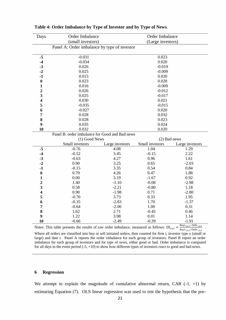
become net buyers around earnings announcements. Panel A in Table (4) reports order

imbalance according to the type of investor. Assuming that different investors have different

levels of ability and resources of information regarding the true value of a security, we use

the value of trades to separate small and large investors. If this assumption is valid, we should

observe different behaviour between the two groups. It is worth mentioning that because

event window (-5,+10) is relatively short, we do not aim to examine trading strategy followed

by investors , but instead examine immediate reaction to news.

The small investors order imbalance in Panel A indicates that they tend to buy more

than sell around earnings announcements, whereas large investors tend to sell immediately

after the announcements; they buy every day and sell on days (-3,-2, 1, 2 and 5). Panel B

shows the order imbalance split further by type of news. Good news is reported in subgroup

(1) and bad news in subgroup (2). The good news portfolio shows interesting results: while

large investors are mainly net-buyers in the pre-announcement period and net-sellers in most

days after the announcement, small investors are net-buyers in the days immediately

following the release of the news. The bad news portfolio in subgroup (2) indicates

concentrated selling for small investors in days (1), (2) and 3), while large investors show no

strong pattern of selling around earnings announcements. The evidence suggests that small

investors are less sophisticated in acquiring pre-announcement information and in

interpreting news. Good news shows strong buying from small investors, while bad news

shows strong selling by small investors. Conversely, large investors show that they buy

shares in good news firms even before the announcement day and sell them afterwards.

Moreover, large investors show a buying pattern on the day of bad news announcements and

the next day. The evidence suggests informed trading and a higher ability to interpret news

among large investors in the SSM. Our results are in some ways similar to those reported by

Barber and Odean (2008), who surmise that individuals tend to be net-buyers whether the

news is good or bad. Their buying behaviour is motivated by the attention-grabbing

20

hypothesis, under which any stock in the news experiences higher abnormal buying. Our

order imbalance results are also similar to those found in Shanthikumar (2004) and Chiang

and Wang (2007), who use similar methodology and find that small investors in general react

more strongly to earnings surprises than do large investors. Moreover, our results suggest that

informed trading is associated with the size of the trades, evidenced by the buying of good

news stocks by large investors in the pre-announcement period.

21

Table 4: Order Imbalance by Type of Investor and by Type of News.

Days Order Imbalance

(small investors)

Order Imbalance

(Large investors) Panel A: Order imbalance by type of investor

-5 -0.031

-0.034 0.026

0.025

0.015 0.023

0.016

0.026

0.025 0.030

-0.035

-0.027 0.028

0.028

0.035 0.032

0.023

0.020 -0.019

-0.009

0.020 0.028

-0.009

-0.012

-0.017 0.021

-0.015

0.020 0.032

0.023

0.024 0.020

-4

-3

-2

-1

0

1

2

3

4

5

6

7

8

9

10

Panel B: order imbalance for Good and Bad news

(1) Good News (2) Bad news

Small investors Large investors Small investors Large investors

-5 -0.76 4.08 1.04 1.29

-4 -0.52 3.45 -0.15 2.22

-3 -0.63 4.27 0.96 1.61

-2 0.90 3.25 0.65 -2.03

-1 -0.15 3.35 0.54 0.84

0 0.79 4.26 0.47 1.88

1 0.00 3.19 -1.67 0.92

2 1.40 -1.10 -0.08 -2.98

3 0.58 -2.21 -0.80 1.18

4 0.90 -1.98 0.71 -2.80

5 -0.70 3.73 0.33 1.95

6 -0.35 -2.83 1.70 -1.37

7 -0.64 -2.00 1.00 0.31

8 1.62 2.71 -0.45 0.46

9 1.22 3.98 0.01 1.14

10 -0.66 -2.49 -0.39 -1.91

Notes: This table presents the results of raw order imbalance, measured as follows: OIi.x.t =Buys i ,x ,t−Sells i ,x ,t

Buys i ,x ,t +Sells i ,x ,t .

Where all orders are classified into buy or sell initiated orders, then counted for firm i, investor type x (small or

large) and date t. Panel A reports the order imbalance for each group of investors. Panel B report an order

imbalance for each group of investors and for type of news, either good or bad. Order imbalance is computed

for all days in the event period (-5, +10) to show how different types of investors react to good and bad news.

6 Regression

We attempt to explain the magnitude of cumulative abnormal return, CAR (-1, +1) by

estimating Equation (7). OLS linear regression was used to test the hypothesis that the pre-

22

announcement stock behaviour and level of trading activity have an effect on the magnitude

of the abnormal returns on the announcement day. We use Cumulative Abnormal Return

(CAR) in the window (-1, +1) to capture the market reaction of the announcement. Then, We

regress CAR on a set of variables which is expected to affect the magnitude of the stock

return. For the pre-announcement explanatory variables, We include the price trend in the

stock returns (momentum), cumulative overnight indicator, average abnormal volume. All

the previous variables are computed using a time frame of the three weeks before the

announcement day, that is, 15 trading days. We also include two firm characteristics; size

measured in market value and the earnings surprise of the current quarter compared to same

quarter of the previous year. Good (Bad) news portfolios contain all the companies which

have positive (negative) CAR (-1, +1).

The aim is to test whether the level of pre-announcement trading activity or firm

characteristic would have predictive power to explain the magnitude of the earnings

announcement returns.

We expect a positive relationship, positive (negative) coefficient estimates for the

good (bad) subsamples for pre-announcement trading activity and the earnings surprise with

regard to abnormal return. At the same time, we expect a negative relationship between firm

size and the magnitude of price reaction CAR that is a negative (positive) coefficient sign for

the good (bad) subsamples.

A cross-sectional model is used to investigate the association between the absolute

CARs and a set of pre-announcement variables covering trading activity and firm

characteristics (Size and SUE) specific to the event observation. The model is constructed as

follows:

𝑪𝑨𝑹𝒊 = 𝜶 + 𝜷𝟏𝑴𝒐𝒎𝒆𝒏𝒕𝒖𝒎𝒊,𝒕 + 𝜷

𝟐𝑶𝑵𝑰𝒊 + 𝜷

𝟑 𝑨𝒃𝒗𝒐𝒍

𝒊 + 𝜷𝟒𝑺𝑼𝑬𝒊,𝒕 + 𝜷

𝟓𝑺𝒊𝒛𝒆𝒊,𝒕

+ 𝜺𝒊,𝒕

(7)

where:

1-Momentum is defined as the compounded stock returns for the past three trading weeks

before the earnings announcement, where: 𝑀𝑜𝑚𝑒𝑛𝑡𝑢𝑚𝑖,𝑡 = 𝑅𝑖 ,𝑡15𝑡=1 and 𝑅𝑖,𝑡 is the daily

stock return for firm i and day t in the window [-16,-2].

23

2-ONI is the summation of overnight indicators over the period [-16,-2] calculated as:

𝑂𝑁𝐼𝑖 = 𝑙𝑜𝑔𝑂𝑝𝑒𝑛

𝑡

𝐶𝑙𝑜𝑠𝑒𝑡−1

15

𝑡=1

(8)

3- 𝐴𝑏𝑣𝑜𝑙 is the average normalised abnormal volume which was first used by Jarrell and

Poulsen (1989). It is computed as the residual of daily volume less mean daily volume scaled

by trading volume standard deviation during the three weeks before an announcement [-16,-

2] as follows:

𝐴𝑏𝑣𝑜𝑙𝑖 ,𝑡 =𝑇𝑉𝑖,𝑡−𝑇𝑉 𝑖,𝑡

𝜎𝑖 ,𝑡 , where 𝑇𝑉

𝑖 ,𝑡 =1

20 𝑇𝑉𝑖 ,𝑡

20𝑡=1 , is the average trading volume for

20 days over the window of [-36,-17] and 𝜎𝑖 ,𝑡 = 1

20 𝑇𝑉𝑖,𝑡 − 𝑇𝑉𝑖,𝑡

220

𝑡=1 , is the standard

deviation of trading volume during the estimation period [-36,-17]. The daily estimated

Abvol is then averaged as follows:

𝐴𝑏𝑣𝑜𝑙

𝑖 =1

15 𝐴𝑏𝑣𝑜𝑙

15

𝑡=1

(9)

4- Standard unexpected earnings (SUE) are measured by scaling the unexpected earnings

(seasonal random walk with a drift) to its standard deviation. The SUE for each firm i at

quarter t is given by:

𝑆𝑈𝐸𝑖,𝑡 =𝑒𝑖,𝑡 − 𝐸(𝑒𝑖,𝑡)

𝜎𝑖,𝑡

(10)

where ei,t represents actual earnings and E(ei,t) is the expected earnings computed using a

random walk model with drift E ei,t = et−4i + δi , where δi is the seasonal drift in a firm‟s

earnings and σi,t is estimated using the figures for the previous 8 quarters‟ earnings.

5- Finally, Size variable is the market value of each firm at the time of the announcement. We

multiply the number of outstanding shares by the closing price immediately before the

earnings announcement day.

24

Table 1: Cross-sectional Regression of Cumulative Abnormal Returns on Pre-

announcement trading activity and Firm Characteristics.

(1) (2)

VARIABLES Good News Bad News

Momentum 0.0140*** -0.00840**

(0.00538) (0.00416)

ONI 0.000215** -0.000218***

(0.000101) (4.67e-05)

𝑨𝒃𝒗𝒐𝒍 0.000328** -0.000272**

(0.000128) (0.000109)

SUE -0.000153* 0.000134***

(5.95e-05) (4.26e-05)

size -0.00130*** 0.00126***

(0.000403) (0.000327)

Constant 0.0402*** -0.0394***

(0.00907) (0.00733)

Observations 860 1131

R-squared 0.058 0.065

Note: This table presents regression coefficients of the earnings announcement returns CAR (-1, +1) on trading activity and firm characteristics for two types of disclosure (Good and Bad news portfolios) for 95 firms during the period 2002-2009 with 1991 as the total number of observations. Good (bad) news firms are defined according to the price reaction during the event window (-1, +1), while positive (negative) CARs are placed in the good (bad) news portfolios. *** p<0.01,*p<0.05, * p<0.1. Standard errors are in parentheses.

As expected, all trading activity variables have a positive relationship with CAR for both

types of news, good and bad. The price trend (momentum) has a positive relationship,

positive (negative) coefficients with good (bad news) firms. The momentum was selected to

show any pre-announcement trend in informed trading. A company which exhibited a price

trend before the release of its earnings shows higher cumulative abnormal returns. However,

the coefficient is higher for the good news firms at 1.4%, suggesting that traders in the good

news firms engage actively in private information seeking. The ONI, which is a measure of

investors‟ disagreement and information asymmetry in the market, also has a positive

relationship with abnormal returns. In the two portfolios, the abnormal volume increases

CAR and is significant at 5%. SUE shows a bizarre negative relationship which is not

expected, with significant coefficients at 10% and 1% for the good and bad news,

respectively. SUE was measured using the seasonal random walk model, since analysts‟

forecasts are not available in the SSM. The time-series model has proven to be inaccurate,

more precisely in the case of the Saudi market, where during the period of our study, the

25

price of oil and earnings per share (EPS) for the whole market rose to more than 400%

between 2002 and 2009. Finally size, as expected, is negatively related to the cumulative

abnormal returns, with positive (negative) coefficients for the bad (good) news which are

significant at 1%. Larger companies in the SSM have substantial government and institution

ownership and have better disclosure practices, which reduces information asymmetry and

the reaction to news for such stocks. In general, pre-announcement trading activity and

information asymmetry (momentum, overnight indicator and volume) have a positive

relationship with cumulative abnormal returns. However, firm characteristics (SUE and Size)

have a negative relationship with CAR.

Liquidity, Information asymmetry around earnings announcement

We first examine the change in liquidity (models 1 & 2 in table 6) around earnings

announcements using an approach similar to that of Venkatesh and Chiang (1986) and Chan

and Chunyan (2005), who examine the change in adverse selection cost around earnings

announcements. We use the estimated bid-ask spread as a proxy for liquidity. Model (1) uses

the effective estimated spread from the model of George et al. (1991) and model (2) uses a

relative estimated spread which deflates the spreads relative to prices. We use the estimated

information asymmetry component of the spread in model (3), where we distinguish adverse

selection cost behaviour with regard to good news and bad news firms. For each earnings

announcement, we estimate the following regression model:

𝑩𝑨𝑺𝒊𝒕 = 𝜶 + 𝜷

𝟏𝑽𝒐𝒍𝒂𝒕𝒊𝒍𝒊𝒕𝒚

𝒊𝒕+ 𝜷

𝟐𝑷𝒓𝒊𝒄𝒆𝒊𝒕 + 𝜷

𝟑 𝑽𝒐𝒍𝒖𝒎𝒆𝒊𝒕 + 𝜷

𝟒𝑫𝟏𝒊𝒕 + 𝜷

𝟓𝑫𝟐𝒊𝒕

+ 𝑩𝟔𝑫𝟑𝒊𝒕 + 𝜺𝒊𝒕

(11)

where:

𝐵𝐴𝑆𝑖𝑡 = Estimated spread of firm i on day t;

𝑉𝑜𝑙𝑎𝑡𝑖𝑙𝑖𝑡𝑦𝑖𝑡 = High to low price range divided by low prices for firm i on day t;

𝑃𝑟𝑖𝑐𝑒𝑖𝑡= closing stock prices of firm i on day t;

𝑉𝑜𝑙𝑢𝑚𝑒𝑖𝑡 =Ln (number of shares traded of firm i on day t multiplied by 𝑃𝑟𝑖𝑐𝑒𝑖𝑡 );

D1it =1 for days -20 to - 2; zero otherwise (pre-announcement period);

D2it =1 for days - 1 to +1; zero otherwise (announcement period);

D3it =1 for days +2 to +20; zero otherwise (post-announcement period).

Following the research design of Venkatesh and Chiang (1986) and Chan and Chunyan

(2005), volatility, price and volume are used in the model to measure the inventory and order

26

processing cost, as suggested by the literature. Dummy variables measure the change in

information asymmetry in the period before, during and after earnings announcements. An

increase in the volatility of a stock will increase its market risk, which would be reflected in

market makers/participants increasing the spread. Therefore, in line with the literature, we

expect volatility to widen the spread because the SSM is an order driven market which has no

designated market makers. Price is assumed to have a negative relationship with regard to

spread because order-processing costs are disproportionately higher for lower priced stocks

(Demsetz, 1968). We also expect a negative relationship between the “Saudi Riyal” trading

volume and the spread, because inventory and liquidation cost will decline with higher

trading. The dummy variables are constructed to test how the information asymmetry

component would affect the spread around earnings announcements. After controlling for

other components of the spread, namely, the inventory and order processing costs, the higher

level of information asymmetry should be reflected in positive coefficients between the bid-

ask spread and the dummy variable.

27

Table 2: Liquidity and Information Asymmetry around Quarterly Earnings

Announcements.

(1) (2) (3)

VARIABLES Spread Relative

Spread

Information Asymmetry

Good Bad

Volatility -2.062*** -0.0407***

(0.0206) (0.000756)

Price -0.00478*** -0.000175***

(1.48e-05) (5.43e-07)

Volume -0.0177*** -0.000121***

(0.000457) (1.68e-05)

D1 -0.000505 -7.88e-05 0.0291*** -0.00746

(0.00158) (5.79e-05) (0.00884) (0.00869)

D2 0.00991*** 0.000312*** 0.0303** 0.0148

(0.00247) (9.09e-05) (0.0128) (0.0127)

D3 0.00961*** 0.000271*** 0.0175* -0.0171**

(0.00157) (5.79e-05) (0.00889) (0.00864)

Constant 1.216*** 0.0266*** 0.370*** 0.754***

(0.00755) (0.000278) (0.0444) (0.0459)

Observations 105827 105827 58965 58110

R-squared 0.573 0.531 0.651 0.689

Notes: This table presents the estimated coefficients of the liquidity and information asymmetry components of volatility, stock price, volume and time dummies, representing the pre-announcement (D1), announcement (D2) and post-announcement periods (D3). Model (1) is run for the estimated spread, Model (2) uses relative spread (spread/price) and Model (3) uses the estimated adverse selection component of the spread as a dependent variable, which was run separately for the good and bad news portfolios. *** p<0.01, ** p<0.05, * p<0.1. Standard errors in parentheses

As expected, spread is negatively associated with stock price and “Saudi Riyal” trading

volume. However, volatility deviates from expectation and shows a negative coefficient too

which could be a reflection of noise trading. A lot of noise trading is expected during this

time.

Controlling for the previous variables should mainly control for the inventory and order

processing components of the spread. The dummy variables show an increasing information

asymmetry around and after earnings announcements (D2 and D3) with positive coefficients

of around 0.01 which are significant at the 1% level. The information asymmetry in the pre-

announcement period (D1) shows negative coefficient, but this is not significant. In general,

28

information asymmetry remains at a high level after the announcement. These results are

consistent with previous literature, maintaining that the different levels of ability among

traders to interpret news aggravate the information asymmetry between them.

Model (3) was used to confirm our original model of the spread around earnings

announcements; this model uses dummies to control for the adverse selection component. In

the information asymmetry model, we use an adverse selection component which was

estimated using the model of George et al (1991) and run the same model again on time

dummies. We show whether this component would differ from or confirm the behaviour of

the spread and time dummies in models 1 and 2. The behaviour of the information

asymmetry component of the spread is reported for three periods, the pre-announcement

period (D1), announcement period (D2) and post-announcement (D3). Regression was run

separately for good news and bad news. Good and bad news firms were defined according to

the earnings announcement return (EAR). Positive (negative) EAR is allocated in good (bad)

groups. Because we are interested only in the information asymmetry component around

earnings announcements, we report the dummies‟ coefficients and ignore the other

coefficients of volatility, price and volume.

The behaviour of information asymmetry differs slightly in model (3) from that in the

previous models, where information increased around and after the date of the earnings

announcement. When we run the information asymmetry component and take into

consideration the nature of the news, new and interesting results emerge. The good news

firms show an increasing positive relationship of information asymmetry relative to the time

of the announcement: information asymmetry gradually increases in the 20 days event

window before the news and then peaks at the announcement period. Information asymmetry

is then reduced after the announcement to the lowest level in the 20 days event window. The

time dummy coefficient is statistically significant at the 1%, 5% and 10 % levels for D1, D2

and D3, respectively. Information asymmetry is reduced substantially in the post-

announcement period, suggesting that earnings announcements reduce uncertainty in the

market. The bad news firms show different behaviour patterns for information asymmetry.

Information asymmetries are at their highest level during the announcement period D2; the

other two periods exhibit lower levels of information asymmetry. However, only period D3

shows a negative coefficient of (-.017) which is significant at the 1% level.

29

The difference between good and bad news information asymmetry supports our conclusion

in the price reaction regression, where we find that traders engage more actively in

information seeking activities in the good news firms. The evidence suggests that while

other components of the spread, inventory and order processing are reduced around the time

of earnings announcements, information asymmetry increases around this time.

Our results are consistent with those of Chan and Chunyan (2005), who also find evidence of

an increase in adverse selection cost around earnings announcements, using similar time

dummies to show an information asymmetry reaction to earnings news.

7 Summary

This study analyses abnormal returns, trading activity (dollar volume, turnover and number

of trades), and liquidity and information asymmetry for the Saudi stock market around its

quarterly earnings announcements. We use a sample of 2,437 quarterly earnings

announcements which covers all listed and operating firms in the period from 2002-2009. We

examine the market reaction to news through computing market adjusted abnormal returns

over various event windows. We also examine the changes in different measurements of

trading activity, liquidity, volatility, asymmetric information and in the traders‟ order

placement strategies. In general, we find a significant increase in abnormal returns, increases

in trading volume, a significant shift in systematic risk, widening bid-ask spread and above

average stock price variability.

The highly significant abnormal returns around earnings announcements indicate the

importance and informativeness of the information content of these announcements. We

observe a rise in trading activities and volatility around earnings announcement with a higher

information asymmetry which gradually reduces in the 20 days following the announcement

date. The persistence of volatility and information asymmetry in the post announcement

period can be explained by the heterogeneity in investors‟ ability to process the information

in the public announcement, which indicates that investors may respond differently to news.

When examining trading behaviour among small and large investors in the market through

order imbalance measures, we find that large investors are more sophisticated and show

higher informed trading before earnings announcements, whereas smaller investors show a

stronger reaction to news. Moreover, small investors show a buying pattern which is

30

consistent with the earnings surprise. Our investors trading placements around earnings

announcements is similar to those found Barber and Odean (2008) and Hirshleifer et al.

(2008). However, we find that small investors are net-buyers for the good news and net-

sellers for the bad news in the 3 days following earnings releases.

We investigate further the magnitude of the cumulative abnormal returns (CAR) and

find it to be positively related to information asymmetry and trading activity in the pre-

announcement period (15 trading days before earnings announcements). CAR is reduced by

the size of the company: larger companies which have higher institutional ownership and

better disclosure practices show a lower CAR around earnings announcement. Surprisingly,

CAR seems to converse effect of the time-series earnings surprise, SUE. One explanation of

this relationship is that time-series coefficients show downward bias in their estimating of the

earnings forecasts, since the market shows an exceptionally high growth in EPS for the years

2002-2009. Hence, SUE does not accurately measure the earnings surprise in the SSM.

Finally, liquidity measured by the bid-ask spread is negatively associated with stock

return volatility, stock price level and riyal trading volume. The time dummy variables which

control for other spread components and test for information asymmetry indicate increasing

spread around the date of earnings announcements which remains relatively high in the

following 20 days. An earnings release as suggested by Kim and Verrecchia (1994)

motivates informed judgement, creating information asymmetry between traders in the

market which can lasts for some time after the announcement.

31

References

1. ACKER, D., 2002. Implied standard deviations and post-earnings announcement volatility. Journal of Business Finance & Accounting, 29(3&4), 429-456.

2. AFFLECK-GRAVES, J., CALLAHAN, C.M. and CHIPALKATTI, N., 2002. Earnings

predictability, information asymmetry and market liquidity. Journal of Accounting Research, 40(3), 561-583.

3. BAKER, M. and STEIN, J.C., 2004. Market liquidity as a sentiment indicator. Journal of Financial

Markets, 7(3), 271-299.

4. BALL, R., 1992. The Earnings-Price Anomaly. Journal of Accounting and Economics, 15(2/3), 319–45.

5. BALSAM, S., BARTOV, E. and MARQUARDT, C., 2002. Accruals management, investor

sophistication and equity valuation: Evidence from 10-Q filings. Journal of Accounting Research, 40(4), 987-1012.

6. BARBER, B.M. and ODEAN, T., 2008. All that glitters: The effect of attention and news on the

buying behavior of individual and institutional investors. Review of Financial Studies, 21(2), 785-818.

7. BEAVER, W.H., 1968. The information content of annual earnings announcements. Journal of

Accounting Research, 6(3), 67-92.

8. BERKMAN, H., DIMITROV, V., JAIN, P.C., KOCH, P.D. and TICE, S., 2009. Sell on the news: Differences of opinion, short-sales constraints and returns around earnings announcements.

Journal of Financial Economics, 9(3), 376-399.

9. BERNARD, V.L. and THOMAS, J., 1989. Post-earnings-announcement drift: Delayed price response or risk premium. Journal of Accounting Research, 27(1), 1-48.

10. BONNER, S.E., WALTHER, B.R. and YOUNG, S.M., 2003. Sophistication-related differences in

investors' models of the relative accuracy of analysts' forecast revisions. The Accounting Review, 78(3), 679-706.

11. BUSHEE, B.J., MATSUMOTO, D.A. and MILLER, G.S., 2003. Open versus closed conference

calls: the determinants and effects of broadening access to disclosure. Journal of Accounting and

Economics, 34(1-3), 149-180. 12. CALLEN, J.L., HOPE, O.K. and SEGAL, D., 2005. Domestic and foreign earnings, stock return

variability and the impact of investor sophistication. Journal of Accounting Research, 43(3), 377-

412. 13. CHIANG,M.H.,Wang.J.Y., 2007. Information Asymmetry and Investors behavior around earnings

announcements. working paper edn. Vienna, Austria: European Financial Management

Association.

14. CHORDIA, T., ROLL, R. and SUBRAHMANYAM, A., 2005. Evidence on the speed of convergence to market efficiency. Journal of Financial Economics, 76(2), 271-292.

15. COLLER, M. and YOHN, T.L., 1997. Management forecasts and information asymmetry: An

examination of bid-ask spreads. Journal of Accounting Research, 35(2), 181-191. 16. DEMSETZ, H., 1968. The Cost of Transacting. The Quarterly Journal of Economics, 82(1), 33-53.

17. FRAZZINI, A. and LAMONT, O.A., 2007. The earnings announcement premium and trading

volume. NBER working paper. 18. GALLO, G.M. and PACINI, B., 2000. The effects of trading activity on market volatility. The

European Journal of Finance, 6(2), 163-175.

19. GEORGE, T.J., KAUL, G. and NIMALENDRAN, M., 1991. Estimation of the bid-ask spread and

its components: A new approach. Review of Financial Studies, 4, 623-656. 20. GLOSTEN, L.R. and HARRIS, L., 1988. Estimating the components of the bid-ask spread.

Journal of Financial Economics, 21(1), 123-142.

21. GREGORIOU, A., IOANNIDIS, C. and SKERRATT, L., 2005. Information Asymmetry and the Bid-Ask Spread: Evidence from the UK. Journal of Business Finance & Accounting, 32(9-10),

1801-1826.

22. GRINBLATT, M. and KELOHARJU, M., 2000. The investment behavior and performance of

various investor types: a study of Finland's unique data set. Journal of Financial Economics, 55(1), 43-67.

32

23. HAKANSSON, N.H., 1977. Interim disclosure and public forecasts: An economic analysis and a framework for choice. Accounting Review, 52(2), 396-426.

24. HAND, J.R.M., 1990. A test of the extended functional fixation hypothesis. Accounting Review,

65, 740-763.

25. HANDA, P., SCHWARTZ, R. and TIWARI, A., 2003. Quote setting and price formation in an order driven market. Journal of Financial Markets, 6(4), 461-489.

26. HAYN, C., 1995. The information content of losses. Journal of Accounting and Economics, 20(2),

125-153. 27. HIRSHLEIFER, D., MYERS, J., MYERS, L.A. and TEOH, S.H., 2008. Do individual investors

drive post-earnings announcement drift? working paper. Electronic copy available at:

http://ssrn.com/abstract=1120495.

28. JARRELL, G.A. and POULSEN, A.B., 1989. The returns to acquiring firms in tender offers: Evidence from three decades. Financial Management, 18(3), 12-19.

29. KARPOFF, J.M., 1986. A theory of trading volume. Journal of Finance, 41, 1069-1087.

30. KIM, O. and VERRECCHIA, R.E., 1994. Market liquidity and volume around earnings announcements. Journal of Accounting and Economics, 17(1), 41-67.

31. KRINSKY, I. and LEE, J., 1996. Earnings announcements and the components of the bid-ask

spread. Journal of Finance, 51, 1523-1535. 32. LAKHAL, F., 2008. Stock market liquidity and information asymmetry around voluntary earnings

disclosures: New evidence from France. International Journal of Managerial Finance, 4(1), 60-75.

33. LEUZ, C. and VERRECCHIA, R.E., 2000. The economic consequences of increased disclosure.

Journal of Accounting Research, 38 (Supplement), 91-124. 34. MUCKLOW, B. and READY, M.J., 1993. Spreads, depths and the impact of earnings

information: An intraday analysis. Review of Financial Studies, 6(2), 345-374.

35. SHANTHIKUMAR, D.M., 2004. Small and large trades around earnings announcements: Does trading behavior explain post-earnings-announcement drift? Working paper, edn. University of

Stanford.

36. VAN NESS, B.F., VAN NESS, R.A. and WARR, R.S., 2001. How well do adverse selection components measure adverse selection? Financial Management, 30(3), 77-98 .

37. VENKATESH, P.C. and CHIANG, R., 1986. Information asymmetry and the dealer's bid-ask

spread: A case study of earnings and dividend announcements. Journal of Finance, 41, 1089-1102.

38. WALTHER, B.R., 1997. Investor sophistication and market earnings expectations. Journal of Accounting Research, 35(2), 157-179.

39. WELKER, M., 1995. Disclosure policy, information asymmetry and liquidity in equity markets.

Contemporary Accounting Research, 11(2), 801-828.

33

Appendix

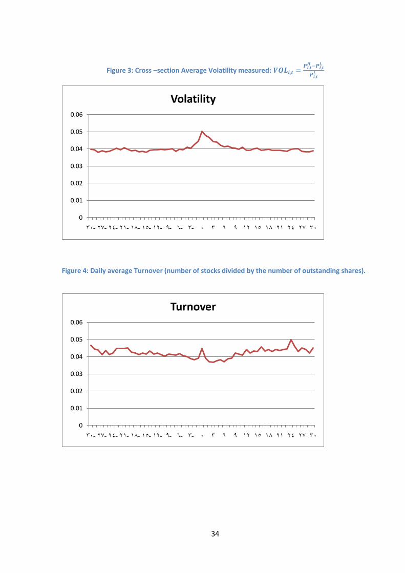
The following graphs depict the daily cross-section average of all observations for the event

window (-30,+30) for 2179 earnings announcements.

Figure 1: Daily estimated Average Bid-Ask Spread using the model of

George et al. (1991)

Figure 2 : Daily Overnight Indicator measured as: 𝑶𝑵𝑰𝒕 = 𝒍𝒐𝒈𝑶𝒑𝒆𝒏𝒕

𝑪𝒍𝒐𝒔𝒆𝒕−𝟏

0.6

0.62

0.64

0.66

0.68

0.7

0.72

0.74

-30 -27 -24 -21 -18 -15 -12 -9 -6 -3 0 3 6 9 12 15 18 21 24 27 30

Bid- Ask Spread

-0.002

-0.001

0

0.001

0.002

0.003

0.004

0.005

0.006

-30 -27 -24 -21 -18 -15 -12 -9 -6 -3 0 3 6 9 12 15 18 21 24 27 30

Overnight Indicator

34

Figure 3: Cross –section Average Volatility measured: 𝑽𝑶𝑳𝒊,𝒕 =𝑷𝒊,𝒕

𝑯 −𝑷𝒊,𝒕𝑳

𝑷𝒊,𝒕𝑳

Figure 4: Daily average Turnover (number of stocks divided by the number of outstanding shares).

0

0.01

0.02

0.03

0.04

0.05

0.06

-30 -27 -24 -21 -18 -15 -12 -9 -6 -3 0 3 6 9 12 15 18 21 24 27 30

Volatility

0

0.01

0.02

0.03

0.04

0.05

0.06

-30 -27 -24 -21 -18 -15 -12 -9 -6 -3 0 3 6 9 12 15 18 21 24 27 30

Turnover

35

Figure 5: Average Number of trades per day

Figure 6: Average Abnormal Returns for all earnings announcements (2,437) before data cleaning

164

166

168

170

172

174

176

178

180

182

184

186

-30 -27 -24 -21 -18 -15 -12 -9 -6 -3 0 3 6 9 12 15 18 21 24 27 30

Number of Trades

-0.008

-0.006

-0.004

-0.002

0

0.002

0.004

0.006

-30 -27 -24 -21 -18 -15 -12 -9 -6 -3 0 3 6 9 12 15 18 21 24 27 30

Abnormal Returns