what controls the mean depth of the pbl? - ucla ... controls the mean depth of the pbl? brian...

What Controls the Mean Depth of the PBL?

BRIAN MEDEIROS, ALEX HALL, AND BJORN STEVENS

Department of Atmospheric and Oceanic Sciences, University of California, Los Angeles, Los Angeles, California

(Manuscript received 2 September 2004, in final form 21 December 2004)

ABSTRACT

The depth of the planetary boundary layer (PBL) is a climatologically important quantity that hasreceived little attention on regional to global scales. Here a 10-yr climatology of PBL depth from theUniversity of California, Los Angeles (UCLA) atmospheric GCM is analyzed using the PBL mass budget.Based on the dominant physical processes, several PBL regimes are identified. These regimes tend toexhibit large-scale geographic organization. Locally generated buoyancy fluxes and static stability controlPBL depth nearly everywhere, though convective mass flux has a large influence at tropical marine loca-tions. Virtually all geographical variability in PBL depth can be linearly related to these quantities. Whiledry convective boundary layers dominate over land, stratocumulus-topped boundary layers are most com-mon over ocean. This division of regimes leads to a dramatic land–sea contrast in PBL depth. Diurnaleffects keep mean PBL depth over land shallow despite large daytime surface fluxes. The contrast arisesbecause the large daily exchange of heat and mass between the PBL and free atmosphere over land is notpresent over the ocean, where mixing is accomplished by turbulent entrainment. Consistent treatment ofremnant air from the deep, daytime PBL is necessary for proper representation of this diurnal behavior overland. Many locations exhibit seasonal shifts in PBL regime related to changes in PBL clouds. These shiftsare controlled by seasonal variations in buoyancy flux and static stability.

1. Introduction

The planetary boundary layer (PBL) is a critical com-ponent of earth’s climate system. It mediates the ex-changes of heat, momentum, moisture, and chemicalconstituents between the surface and free atmosphereand is the largest sink for atmospheric kinetic energy.Boundary layer processes are also primarily responsiblefor low clouds like stratocumulus and are of fundamen-tal importance for cumulus convection, implying thatthe PBL has important roles in both the atmosphericradiative and heat budgets. Because of this crucial role,there is general agreement that large-scale models mustinclude some representation of boundary layer pro-cesses to simulate essential climatic quantities like glob-al cloudiness, precipitation, and surface winds.

PBL parameterizations are often based around a fewboundary layer regimes. Figure 1 is an idealized sche-matic depicting a variety of these regimes and the large-scale environment thought to be conducive to their for-mation (see also Lock et al. 2000). On the left-hand side

are regimes with large surface latent heat and convec-tive mass fluxes, where active cumulus convection cov-ers a few percent of the area. The other cloudy bound-ary layers occur over cooler sea surfaces and mostlyexist under an inversion related to the subsiding branchof the Hadley–Walker circulation, encouraging morehomogeneous cloud coverage. Two kinds of clear PBLare shown over land: the stable boundary layer (SBL)and the (dry) convective boundary layer (CBL). SBLsoccur most often over cold surfaces or during nighttimeover land; CBLs are the dominant PBL regime overland during daytime, when surface fluxes drive convec-tive updrafts. Farthest to the right in the figure is afair-weather cumulus boundary layer, with a CBL be-low shallow cumulus.

There are now detailed datasets describing the PBLunder various large-scale conditions. Intensive observa-tional campaigns have been undertaken over diversesurface types in many regions. A few of these observa-tions are listed in Table 1. These and similar data havebeen used in developing large-eddy simulations (LESs)and PBL parameterizations. The local nature of thesekinds of observations, however, makes them most use-ful for understanding particular PBL regimes, not gen-eralized PBL behavior.

Large-scale modeling studies have mostly focused on

Corresponding author address: Brain Medeiros, Department ofAtmospheric and Ocean Sciences, 405 Hilgard Ave., Box 951565,Los Angeles, CA 90095-1565.E-mail: [email protected]

15 AUGUST 2005 M E D E I R O S E T A L . 3157

© 2005 American Meteorological Society

JCLI3417

parameterization validation. These studies sometimescompare observations and large-scale models usingsingle grid points (e.g., Garratt et al. 2002), keepingwith the local view of most observations. Comparisonson large scales are rare because few adequate large-scale PBL observations exist. As part of testing theparameterization of Lock et al. (2000), Martin et al.(2000) include a qualitative comparison with satelliteimagery. Randall et al. (1998) compare two climatemodels to global observations [Comprehensive Ocean–Atmosphere Data Set (COADS) surface fluxes, LidarIn-space Technology Experiment (LITE) PBL depth,and International Satellite Cloud Climatology Project(ISCCP) stratus cloud amount], but few conclusions aredrawn as the focus is on reviewing PBL parameteriza-tions in climate models. Parameterization evaluationsusually show cautious optimism about their relativesuccess, but a true validation must wait for a more com-plete PBL dataset.

Considering the attention given to treatment of thePBL, there is little sense of the global distribution ofPBL depth and its relationship to the large-scale con-ditions. Until now it has been impossible to observe the

large-scale structure of the PBL depth [except theproof-of-concept LITE (McCormick et al. 1993;Winker et al. 1996)]. In coming years though, satelliteremote sensing projects [e.g., Atmospheric InfraredSounder (AIRS); Cloud-Aerosol Lidar and InfraredPathfinder Satellite Observations (CALIPSO); Cloudsand the Earth’s Radiant Energy System (CERES); Ice,Cloud, and Land Elevation Satellite (ICESAT)] are ex-pected to produce global datasets for PBL depth andother boundary layer quantities. As these data becomeavailable, it is valuable to develop an intuition for thelarge-scale behavior of the PBL using large-scale mod-els. This will introduce a framework for integratedanalysis of observations and simulations in a global con-text. A global perspective is desirable for exploring therole of the PBL in global climate and may help in de-veloping simplified PBL representations for idealizedclimate models.

This study utilizes the University of California, LosAngeles (UCLA) atmospheric general circulationmodel (GCM) to reveal the processes regulating PBLdepth on large scales. This GCM is particularly appro-priate for such a study because it goes to extraordinary

FIG. 1. Schematic view of several PBL regimes. From left to right: deep convection, shallowcumulus (Cu), stratocumulus (Sc) decoupled from the subcloud layer, stratocumulus-toppedboundary layer (STBL), stratocumulus overlying a stable boundary layer (SBL), two clearboundary layers (convective and stable), and a fair-weather cumulus boundary layer (FWBL)with a convective subcloud layer and a cumulus cloud layer. The top of the PBL, as definedby the UCLA GCM, is marked by dotted lines, except in the case of the decoupled Sc layer,which is not represented by the model. Dark arrows are representative of the local circulation,with cumulus mass flux removing mass from the PBL in the cumulus regimes and convectivecells in the other convective regimes. Stable boundary layers may be turbulent, but notconvective, so arrows are neglected. The gray arrows pointed downward represent large-scalesubsidence, which tends to increase the static stability.

3158 J O U R N A L O F C L I M A T E VOLUME 18

lengths to consistently couple the budgets of mass, heat,and moisture within the PBL to the processes believedto influence the PBL (e.g., cumulus convection, radia-tive fluxes). This is accomplished using a mixed-layerframework in which PBL depth is a prognostic variable(see section 2). The climatological PBL depth from a10-yr simulation (Fig. 2) is analyzed primarily by exam-ining the PBL mass budget. A simple dry CBL modeland a second GCM simulation excluding the diurnalcycle are also used. The annual mean is the primaryfocus, although both the diurnal and seasonal variationsare important to the mean depth, and so are also studied.

2. Models

This section reviews some aspects of the UCLA at-mospheric GCM relevant for this study. A more com-

plete description is provided by Mechoso et al. (2000)and references therein. This GCM is well suited tostudying PBL processes because it makes use of a modi-fied vertical sigma coordinate in which the PBL is syn-onymous with the lowest model layer. The PBL top actseffectively as a material surface with immediately over-lying coordinate surfaces following the PBL’s verticalvariations and higher levels gradually tending towarduniform pressure surfaces. This configuration wasimplemented by Suarez et al. (1983), incorporating themixed-layer theory of Lilly (1968) and the surface fluxscheme of Deardorff (1972).

This vertical coordinate system distinguishes theUCLA GCM and its descendants from other models.Most GCMs use eddy diffusion models with fixed ver-tical levels to represent boundary effects, and the PBLdepth is often diagnosed separately from the dynamics.These treatments can introduce inconsistencies by fail-ing to ensure that effective mixing rates between thePBL and free troposphere are the same for mass, heat,and moisture. In some models the diagnosed depth isused in the subsequent dynamic time step, but manymodels do not use the depth as a dynamical length scale(see review in Moeng and Stevens 2000). In the UCLAGCM, however, the PBL has been integrated so it isconsistently coupled to processes in the lower tropo-sphere, making it especially useful for investigatingPBL behavior.

Parameterizing stratocumulus clouds is also simpli-fied by this approach. The GCM diagnoses cloud inci-dence by determining the lifting condensation level(LCL) of mixed-layer air and comparing it to the PBLdepth. If the LCL is below the PBL top, stratocumulusare predicted (see Suarez et al. 1983; Li and Arakawa1999; Li et al. 2002 for details). In later sections it isshown that the presence of stratocumulus profoundlyaffects mean PBL depth. Bearing that in mind, it isrelevant that stratocumulus in this GCM are also af-fected by cloud-top entrainment instability (CTEI;Randall 1980; Deardorff 1980). CTEI can dissipate stra-tocumulus by entraining warm, dry air into the PBL,and the assumptions involved may affect the global cli-matology in several ways, which is considered in thefollowing analysis.

One problem introduced by a single-layer PBL is thatsometimes the PBL depth is ambiguous. A prominentexample is deep convection, when the entire tropo-sphere becomes effectively well mixed. To avoid nu-merical problems in such situations, the PBL top is setat cloud base, so the PBL is only the subcloud layer(Fig. 1). As a consequence of this definition, stratocu-mulus layers tend to appear as regions of deep PBL,

TABLE 1. Some field studies with detailed PBL data.

Surface/region Project Reference

Flat grassland FIFEa Sellers et al. (1992)Boreal forest BOREAS Sellers et al. (1995)Amazon basin LBAb Avissar and Nobre

(2002)Eastern Pacific EPIC Bretherton et al. (2004)

DYCOMS-II Stevens et al. (2003)DYCOMS Lenschow et al. (1988)

Western Pacific TOGA COAREc Webster and Lukas(1992)

SubtropicalAtlantic

ASTEXd Albrecht et al. (1995)

Ice-covered seas SHEBAe Uttal et al. (2002)

a First International Satellite Land Surface Climatology Project(ISLSCP) Field Experiment.

b Large Scale Biosphere–Atmosphere Experiment in Amazonia.c Tropical Ocean Global Atmosphere Coupled Ocean–Atmo-

sphere Response Experiment.d Atlantic Stratocumulus Transition Experiment.e Surface Heat Budget of the Arctic Ocean.

FIG. 2. Annual-mean PBL depth (hPa) from the 10-yr GCMsimulation. Contours are every 10 hPa, from 10 to 140 hPa.


while regions dominated by cumulus convection usuallyhave a comparatively shallow PBL. This conventionalso applies to regions of shallow cumulus convection,for example, downstream of stratocumulus decks. TheGCM does not explicitly parameterize shallow convec-tion, but relies on the moist convection scheme andCTEI to capture this regime (see Randall et al. 1985).Occasionally this leads to some discrepancy betweenthe GCM and observed climatologies; usually shallowconvection appears as a shallow PBL with the top atcloud base.

For numerical stability, upper and lower limits areimposed on the PBL depth. The upper limit is 15% ofthe total tropospheric depth. This limit can be circum-vented since the second vertical layer is not required tobe thermodynamically distinct from the PBL (Suarez etal. 1983). The lower limit (10 hPa) avoids difficultieswith horizontal advection in the PBL. Because themodel framework is a mixed-layer approach, stableboundary layers are not well represented. However,since a typical SBL depth is around 10 hPa [e.g., Barrand Betts (1997) report 9–13 hPa during BOREAS], itis assumed that the lower limit represents the stableregime of Fig. 1. The lower limit is most often foundwhere surface temperatures are low and/or where thereis little solar radiation, conditions that promote gravi-tational stability, so the assumption seems reasonable.

For this study, a coarse resolution (4° � 5°) grid isused with climatological SST and sea ice concentration.Most of the analysis uses monthly means calculatedfrom hourly snapshots of the simulation. Additionally,12-times-daily snapshots were saved for one year forexamination of the diurnal cycle. The large grid spacingprecludes discussion of mesoscale (or smaller) featuressuch as the shoaling of the PBL near coastlines wherestratocumulus become thin (Neiburger et al. 1961).Thus the focus is on regional-scale and larger charac-teristics of PBL depth.

To isolate physical processes determining the clima-tological PBL depth and its diurnal variation, a modelof the dry convective PBL was developed. The modeluses prescribed solar forcing and a surface energy bud-get to calculate PBL depth. The surface warms theboundary layer, which grows by a simple entrainmentrule. A slowly cooling residual layer is included abovethe boundary layer to represent remnant air oftenfound above the nocturnal PBL. The advantage of sucha simplified model is its small number of parameters,making interpretation of the results more straightfor-ward than the GCM. This allows dominant processesdetermining PBL depth to be isolated. The details ofthis CBL model are found in the appendix.

3. Mean state of the PBL

a. Mean PBL depth

In Fig. 2 the climatological mean PBL depth is gen-erally much shallower over land than ocean. This runscounter to the intuitive notion of a deep PBL overwarm land regions. The large diurnal variation inground temperature is a key factor in this land–sea con-trast, as will be shown in the next section.

Also evident in Fig. 2 are regions of deep PBL overeastern ocean basins. A comparison with a map of stra-tus incidence (not shown) shows qualitative agreementbetween these regions and high stratus incidence. TheCalifornian and Peruvian stratiform regions have espe-cially deep PBL. The Namibian, Canarian, and Austra-lian stratus are also evident, though less dramatically.Stratocumulus correspond to large PBL depth becauseconvective fluxes raise the PBL top above the LCLwithout initiating deeper convection. When conditionsbecome more favorable for cumulus, the GCM reducesthe PBL top to cloud base (section 2).

At high latitudes, the mean PBL depth is shallow,frequently near the 10 hPa. This shallow layer resultsfrom a cold surface and stable conditions. Occasionallystratocumulus form at these locations, especially overNorthern Hemisphere (NH) land and Southern Hemi-sphere (SH) sea ice (see below), deepening the PBLwhile the clouds persist. Though Fig. 2 suggests theshallow PBL is the dominant regime here, the deeperregime also influences the mean value. This modifica-tion is due to strong seasonal variation, discussed be-low.

b. Seasonal variation

The phase and amplitude of the seasonal variation ofPBL depth in the 10-yr simulation is shown in Fig. 3.For many locations large seasonal variation is associ-ated with changes in PBL regime, which modifies theclimatological depth.

The largest seasonal variation is found over the NHstorm tracks, where the amplitude is �100 hPa, gener-ally exceeding the mean value (�70 hPa). The maxi-mum PBL depth occurs here during boreal autumn andwinter. As cold, continental air is advected over thewarm western boundary currents, the lower atmo-sphere becomes unstable and a deep PBL forms. Thesurface air reaches the LCL and low clouds form, in-terpreted as stratocumulus in the GCM. The resultingstratocumulus-topped boundary layer is thus a strongseasonal phenomena, existing only during the winter-time.

Throughout the SH sea ice region around the Ant-arctic coast, the PBL depth generally reaches its sea-


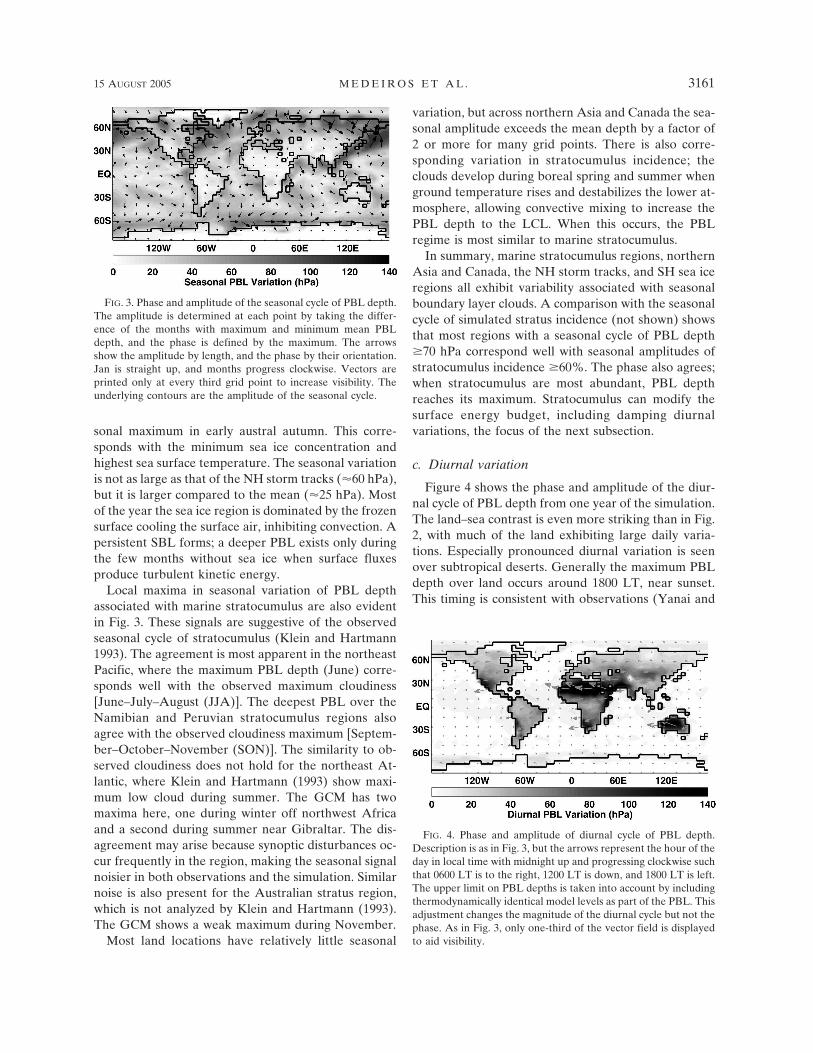
sonal maximum in early austral autumn. This corre-sponds with the minimum sea ice concentration andhighest sea surface temperature. The seasonal variationis not as large as that of the NH storm tracks (�60 hPa),but it is larger compared to the mean (�25 hPa). Mostof the year the sea ice region is dominated by the frozensurface cooling the surface air, inhibiting convection. Apersistent SBL forms; a deeper PBL exists only duringthe few months without sea ice when surface fluxesproduce turbulent kinetic energy.

Local maxima in seasonal variation of PBL depthassociated with marine stratocumulus are also evidentin Fig. 3. These signals are suggestive of the observedseasonal cycle of stratocumulus (Klein and Hartmann1993). The agreement is most apparent in the northeastPacific, where the maximum PBL depth (June) corre-sponds well with the observed maximum cloudiness[June–July–August (JJA)]. The deepest PBL over theNamibian and Peruvian stratocumulus regions alsoagree with the observed cloudiness maximum [Septem-ber–October–November (SON)]. The similarity to ob-served cloudiness does not hold for the northeast At-lantic, where Klein and Hartmann (1993) show maxi-mum low cloud during summer. The GCM has twomaxima here, one during winter off northwest Africaand a second during summer near Gibraltar. The dis-agreement may arise because synoptic disturbances oc-cur frequently in the region, making the seasonal signalnoisier in both observations and the simulation. Similarnoise is also present for the Australian stratus region,which is not analyzed by Klein and Hartmann (1993).The GCM shows a weak maximum during November.

Most land locations have relatively little seasonal

variation, but across northern Asia and Canada the sea-sonal amplitude exceeds the mean depth by a factor of2 or more for many grid points. There is also corre-sponding variation in stratocumulus incidence; theclouds develop during boreal spring and summer whenground temperature rises and destabilizes the lower at-mosphere, allowing convective mixing to increase thePBL depth to the LCL. When this occurs, the PBLregime is most similar to marine stratocumulus.

In summary, marine stratocumulus regions, northernAsia and Canada, the NH storm tracks, and SH sea iceregions all exhibit variability associated with seasonalboundary layer clouds. A comparison with the seasonalcycle of simulated stratus incidence (not shown) showsthat most regions with a seasonal cycle of PBL depth�70 hPa correspond well with seasonal amplitudes ofstratocumulus incidence �60%. The phase also agrees;when stratocumulus are most abundant, PBL depthreaches its maximum. Stratocumulus can modify thesurface energy budget, including damping diurnalvariations, the focus of the next subsection.

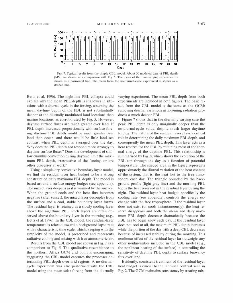
c. Diurnal variation

Figure 4 shows the phase and amplitude of the diur-nal cycle of PBL depth from one year of the simulation.The land–sea contrast is even more striking than in Fig.2, with much of the land exhibiting large daily varia-tions. Especially pronounced diurnal variation is seenover subtropical deserts. Generally the maximum PBLdepth over land occurs around 1800 LT, near sunset.This timing is consistent with observations (Yanai and

FIG. 3. Phase and amplitude of the seasonal cycle of PBL depth.The amplitude is determined at each point by taking the differ-ence of the months with maximum and minimum mean PBLdepth, and the phase is defined by the maximum. The arrowsshow the amplitude by length, and the phase by their orientation.Jan is straight up, and months progress clockwise. Vectors areprinted only at every third grid point to increase visibility. Theunderlying contours are the amplitude of the seasonal cycle.

FIG. 4. Phase and amplitude of diurnal cycle of PBL depth.Description is as in Fig. 3, but the arrows represent the hour of theday in local time with midnight up and progressing clockwise suchthat 0600 LT is to the right, 1200 LT is down, and 1800 LT is left.The upper limit on PBL depths is taken into account by includingthermodynamically identical model levels as part of the PBL. Thisadjustment changes the magnitude of the diurnal cycle but not thephase. As in Fig. 3, only one-third of the vector field is displayedto aid visibility.


Li 1994; Betts et al. 1996; Barr and Betts 1997; LeMoneet al. 2000), though the maximum depth is underesti-mated by the GCM. For example, mixed layers werecommonly observed to reach higher than 3 km duringthe Boreal Ecosystem–Atmosphere Study (BOREAS)(Sellers et al. 1995), while the GCM rarely predicts amaximum PBL depth greater than about 1.5 km for thesame region of Canada.

Comparing two PBL depth time series from July(Fig. 5) illustrates the difference in PBL depth overland and ocean. The land grid point is in the Sahara(26°N, 0°), where high daytime temperatures indicatelarge surface buoyancy flux. This leads to the deep PBLduring the afternoon. The ocean point (22°N, 130°W) isin the northeast Pacific where stratocumulus are com-mon during July. The mean of the Saharan time series(63 hPa) is much smaller than its mean daily maximum(177 hPa), while the marine series maintains a deeperPBL (�127 hPa) and has no diurnal cycle. While theGCM underestimates the daily maximum PBL depthover land, the depth of stratocumulus-topped PBLsseems reasonable. The GCM estimates PBL depth ofaround 1 km in the eastern Pacific (Fig. 2); observationsfrom the second Dynamics and Chemistry of MarineStratocumulus field study (DYCOMS-II) (Stevens etal. 2003) are around 800–900 m, and those from theEastern Pacific Investigation of Climate (EPIC) arecloser to 1200 m (Bretherton et al. 2004).

Both the diurnal and seasonal variation of PBL depthultimately result from the surface response to solarforcing. The contrast between Figs. 3 and 4 highlightsthe difference in the response time scales of ocean andland. Land surfaces have a smaller thermal conductivitythan water, so they respond faster to solar forcing, al-lowing large diurnal variation in ground temperatureand surface heat fluxes. The results shown in this sec-tion show that the land–sea contrast is the primarysource of spatial variability in the climatological PBLdepth, and that it is related to the diurnal variation overland. In the next section the land–sea contrast is exam-ined in detail.

4. The land–sea contrast

To understand the impact of the diurnal cycle onmean PBL depth, a second GCM experiment was per-formed in which the diurnal cycle was removed. Toeliminate diurnal variation, the incoming solar radia-tion was modified so each grid point receives the sameinsolation each day as in the original simulation, butuniformly distributed over 24 h, much like the “toroidalsun” experiment of Randall et al. (1985). The resultingmean PBL depth (Fig. 6) shows a greatly diminishedland–sea contrast compared to Fig. 2; there is little dif-

ference over the ocean, but over land mean PBL depthchanges from 29 to 57 hPa. Over deserts mean PBLdepth more than doubles compared to the control simu-lation. The only land points where PBL depth is unaf-fected are high latitudes where diurnal variation is al-ways small and Amazonia where cumulus convectionwas much more pervasive than in the control simula-tion, keeping the PBL shallow.

The diurnal behavior of the PBL over land is wellknown. In the simplest terms it is characterized by anextremely shallow, shear-driven SBL at night, thedevelopment of a deep convectively mixed structurein the morning and through the day, and a collapseback to a shallow layer after sunset, leaving a warmresidual layer above the nocturnal PBL (cf. Stull 1988;

FIG. 5. Time series of PBL depth for 1 Jul for a grid point in(top) northern Africa and (bottom) the eastern Pacific. The diur-nal cycle of PBL depth is clear for the African point, but is not atall evident for the eastern Pacific. The shallow nocturnal PBL atthe African point brings the mean (horizontal line at 72 hPa) to afairly low value despite the deep daily maxima. The oceanic pointon has a much deeper mean (114 hPa), but less variation. Thedashed lines are the Jul mean from the no-diurnal-cycle experi-ment at the same points.

FIG. 6. Annual-mean PBL depth (hPa) from the 10-yr GCMsimulation with no diurnal variation in solar insolation. The scalecorresponds with that of Fig. 2.


Betts et al. 1996). The nighttime PBL collapse couldexplain why the mean PBL depth is shallower in situ-ations with a diurnal cycle in the forcing, assuming themean daytime depth of the PBL is not substantiallydeeper at the diurnally modulated land locations thanmarine locations, as corroborated by Fig. 5. However,daytime surface fluxes are much greater over land. IfPBL depth increased proportionally with surface forc-ing, daytime PBL depth would be much greater overland than ocean, and there would be little land–seacontrast when PBL depth is averaged over the day.Why does the PBL depth not respond more strongly todaytime surface fluxes? Does the development of shal-low cumulus convection during daytime limit the maxi-mum PBL depth, irrespective of the forcing, or areother processes at work?

Using a simple dry convective boundary layer model,we find the residual-layer heat budget to be a strongconstraint on daily maximum PBL depth. The model isbased around a surface energy budget (see appendix).The mixed layer deepens as it is warmed by the surface.When the ground cools and the heat flux becomesnegative (after sunset), the mixed layer decouples fromthe surface and a cool, stable boundary layer forms.The residual layer is retained as a slowly cooling layerabove the nighttime PBL. Such layers are often ob-served above the boundary layer in the morning (e.g.,Betts et al. 1996). In the CBL model, the residual-layertemperature is relaxed toward a background lapse ratewith a characteristic time scale, which, keeping with thesimplicity of the model, is prescribed and representsradiative cooling and mixing with free atmospheric air.

Results from the CBL model are shown in Fig. 7 as acomparison to Fig. 5. The qualitative resemblance tothe northern Africa GCM grid point is encouraging,suggesting the CBL model captures the processes de-termining PBL depth over arid regions. A no-diurnal-cycle experiment was also performed with the CBLmodel using the mean solar forcing from the diurnally

varying experiment. The mean PBL depth from bothexperiments are included in both figures. The basic re-sult from the CBL model is the same as the GCM:removing diurnal variations in incoming radiation pro-duces a much deeper PBL.

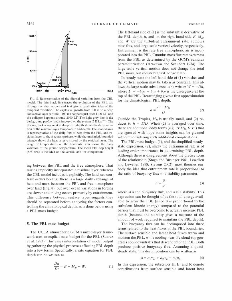
Figure 7 shows that in the diurnally varying case thepeak PBL depth is only marginally deeper than theno-diurnal-cycle value, despite much larger daytimeforcing. The nature of the residual layer plays a criticalrole in determining the daily maximum PBL depth, andconsequently the mean PBL depth. This layer acts as aheat reserve for the PBL by retaining most of the ther-mal energy of the daytime PBL. This relationship issummarized by Fig. 8, which shows the evolution of thePBL top through the day as a function of potentialtemperature. The shaded area in the figure representsapproximately the diurnal variation of the heat contentof the system, that is, the heat lost to the free atmo-sphere each day. The triangle bounded by the back-ground profile (light gray line) and the morning PBLtop is the heat reserved in the residual layer during thenight. The residual-layer heat budget, specifically thecooling rate (see appendix), controls the energy ex-change with the free troposphere. If the residual layerdoes not exist (or cools instantaneously), the heat re-serve disappears and both the mean and daily maxi-mum PBL depth decrease dramatically because thePBL has to begin anew each day. If the residual layerdoes not cool at all, the maximum PBL depth increaseswhile the portion of the day with a deep CBL decreasesbecause of increased stability during the morning. Thisnonlinear effect of the residual layer far outweighs anyother nonlinearities included in the CBL model (e.g.,the nonlinear heating of the surface) in controlling thesensitivity of daytime PBL depth to surface buoyancyflux over land.

Evidently, consistent treatment of the residual-layerheat budget is crucial to the land–sea contrast seen inFig. 2. The GCM maintains consistency by treating mix-

FIG. 7. Typical results from the simple CBL model. About 30 modeled days of PBL depth(hPa) are shown as a comparison with Fig. 5. The mean of the time-varying experiment isshown as a horizontal line. The mean from the no-diurnal-cycle experiment is shown as adashed line.


ing between the PBL and the free atmosphere. Thatmixing implicitly incorporates a residual layer, whereasthe CBL model includes it explicitly. The land–sea con-trast occurs because there is a large daily exchange ofheat and mass between the PBL and free atmosphereover land (Fig. 8), but over ocean variations in forcingare slower and mixing occurs primarily by entrainment.This difference between surface types suggests theyshould be separated before analyzing the factors con-trolling the climatological depth, as is done below usinga PBL mass budget.

5. The PBL mass budget

The UCLA atmospheric GCM’s mixed-layer frame-work uses an explicit mass budget for the PBL (Suarezet al. 1983). This eases interpretation of model outputby gathering the physical processes affecting PBL depthinto a few terms. Specifically, a rate equation for PBLdepth can be written as

Dh

Dt� E � MB � W. �1�

The left-hand side of (1) is the substantial derivative ofthe PBL depth, h, and on the right-hand side E, MB,and W are the turbulent entrainment rate, cumulusmass flux, and large-scale vertical velocity, respectively.Entrainment is the rate free atmospheric air is incor-porated into the PBL. Cumulus mass flux removes massfrom the PBL as determined by the GCM’s cumulusparameterization (Arakawa and Schubert 1974). Thelarge-scale vertical motion does not change the totalPBL mass, but redistributes it horizontally.

In steady state the left-hand side of (1) vanishes andthe vertical motion may be taken as constant. This al-lows the large-scale subsidence to be written W � �Dh,where D � ��zw � �xu � �y is the divergence at thetop of the PBL. Rearranging gives a first approximationfor the climatological PBL depth,

h �E � MB

D. �2�

Outside the Tropics, MB is usually small, and (2) re-duces to h � E/D. When (2) is averaged over time,there are additional eddy terms (e.g., DMB, DE) thatare ignored with hope some insights can be gleanedwithout considering such additional complications.

The PBL mass budget, (1), and the simplified steady-state expression, (2), imply the entrainment rate is ofleading-order importance in determining PBL depth.Although there is disagreement about the precise formof the relationship (Stage and Businger 1981; Lewellenand Lewellen 1998; Stevens 2002), most theories em-body the idea that entrainment rate is proportional tothe ratio of buoyancy flux to a stability parameter,

E �B

�, �3�

where B is the buoyancy flux, and � is a stability. Thisexpression can be thought of as the total energy avail-able to grow the PBL (since B is proportional to theturbulent kinetic energy) compared to the potentialbarrier that must be overcome to actually increase PBLdepth (because the stability gives a measure of theamount of work required to maintain the PBL depth).

The buoyancy flux can be decomposed into threeterms related to the heat fluxes at the PBL boundaries.The surface sensible and latent heat fluxes warm andmoisten the PBL, while cooling near the cloud-top gen-erates cool downdrafts that descend into the PBL. Bothproduce positive buoyancy flux. Assuming a quasi-steady state, this decomposition can be written as

B � �1BH � �2BE � �3BR. �4�

In this expression, the subscripts H, E, and R denotecontributions from surface sensible and latent heat

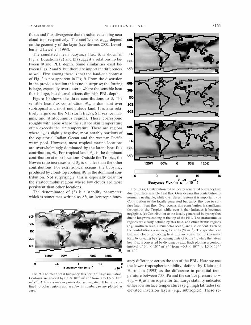
FIG. 8. Representation of the diurnal variation from the CBLmodel. The thin black line traces the evolution of the PBL topthrough the day; arrows and text give a qualitative idea of thetemporal evolution. The explosive growth from 100 m to a deepconvective layer (around 1100 m) happens just after 1100 LT, andthe collapse happens around 2000 LT. The light gray line is thebackground profile that is imposed on the system (5 K km�1). Thethicker, darker segment at deep PBL depth shows the daily varia-tion of the residual-layer temperature and depth. The shaded areais representative of the daily flux of heat from the PBL and re-sidual layer to the free atmosphere, while the unshaded, boundedtriangle shows the heat reserve stored by the residual layer. Therange of temperatures on the horizontal axis shows the dailyvariation of the ground temperature. The mean PBL top height(575 hPa) is included on the vertical axis for comparison.


fluxes and flux divergence due to radiative cooling nearcloud top, respectively. The coefficients �1,2,3 dependon the geometry of the layer (see Stevens 2002; Lewel-len and Lewellen 1998).

The simulated mean buoyancy flux, B, is shown inFig. 9. Equations (2) and (3) suggest a relationship be-tween B and PBL depth. Some similarities exist be-tween Figs. 2 and 9, but there are important differencesas well. First among these is that the land–sea contrastof Fig. 2 is not apparent in Fig. 9. From the discussionin the previous section this is not a surprise; the forcingis large, especially over deserts where the sensible heatflux is large, but diurnal effects diminish PBL depth.

Figure 10 shows the three contributions to B. Thesensible heat flux contribution, BH, is dominant oversubtropical and most midlatitude land. It is also rela-tively large over the NH storm tracks, SH sea ice mar-gins, and stratocumulus regions. These correspondroughly with areas where the surface skin temperatureoften exceeds the air temperature. There are regionswhere BH is slightly negative, most notably portions ofthe equatorial Indian Ocean and the western Pacificwarm pool. However, most tropical marine locationsare overwhelmingly dominated by the latent heat fluxcontribution, BE. For tropical land, BH is the dominantcontribution at most locations. Outside the Tropics, theBowen ratio increases, and BE is smaller than the othercontributions. For extratropical oceans, the buoyancyproduced by cloud-top cooling, BR, is the dominant con-tribution. Not surprisingly, this is especially clear forthe stratocumulus regions where low clouds are morepersistent than other locations.

The denominator of (3) is a stability parameter,which is sometimes written as b, an isentropic buoy-

ancy difference across the top of the PBL. Here we usethe lower-tropospheric stability, defined by Klein andHartmann (1993) as the difference in potential tem-perature between 700 hPa and the surface pressure, � ��700 � �s as a surrogate for b. Large stability indicateseither low surface temperatures (e.g., high latitudes) orelevated inversion layers (e.g., subtropics). These re-

FIG. 9. The mean total buoyancy flux for the 10-yr simulation.Contours are spaced by 0.1 � 10�3 m2 s�3 from 0 to 1.5 � 10�3

m2 s�3. A few anomalous points do have negative B, but are con-fined to polar regions and are few in number, so are plotted aszero.

FIG. 10. (a) Contribution to the locally generated buoyancy fluxdue to surface sensible heat flux. Over oceans this contribution isnormally negligible, while over desert regions it is important. (b)Contribution to the locally generated buoyancy flux due to sur-face latent heat flux. Over oceans this contribution is significantthroughout the Tropics, while over higher latitudes it becomesnegligible. (c) Contribution to the locally generated buoyancy fluxdue to longwave cooling at the top of the PBL. The stratocumulusregions are clearly defined by this field, and other stratus regions(e.g., northern Asia, circumpolar ocean) are also evident. Each ofthe contributions is in energetic units (W m�2). The specific heatflux and cloud-top cooling heat flux are converted to kinematicform by dividing by cp�, leaving units of K m s�1, while the latentheat flux is converted by dividing by L�. Each plot has a contourinterval of 0.1 � 10�3 m2 s�3 from �0.5 � 10�3 to 1.5 � 10�3

m2 s�3.


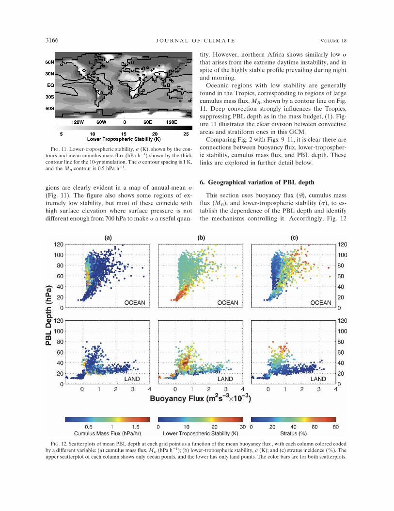
gions are clearly evident in a map of annual-mean �(Fig. 11). The figure also shows some regions of ex-tremely low stability, but most of these coincide withhigh surface elevation where surface pressure is notdifferent enough from 700 hPa to make � a useful quan-

tity. However, northern Africa shows similarly low �that arises from the extreme daytime instability, and inspite of the highly stable profile prevailing during nightand morning.

Oceanic regions with low stability are generallyfound in the Tropics, corresponding to regions of largecumulus mass flux, MB, shown by a contour line on Fig.11. Deep convection strongly influences the Tropics,suppressing PBL depth as in the mass budget, (1). Fig-ure 11 illustrates the clear division between convectiveareas and stratiform ones in this GCM.

Comparing Fig. 2 with Figs. 9–11, it is clear there areconnections between buoyancy flux, lower-tropospher-ic stability, cumulus mass flux, and PBL depth. Theselinks are explored in further detail below.

6. Geographical variation of PBL depth

This section uses buoyancy flux (B), cumulus massflux (MB), and lower-tropospheric stability (�), to es-tablish the dependence of the PBL depth and identifythe mechanisms controlling it. Accordingly, Fig. 12

FIG. 11. Lower-tropospheric stability, � (K), shown by the con-tours and mean cumulus mass flux (hPa h�1) shown by the thickcontour line for the 10-yr simulation. The � contour spacing is 1 K,and the MB contour is 0.5 hPa h�1.

FIG. 12. Scatterplots of mean PBL depth at each grid point as a function of the mean buoyancy flux , with each column colored codedby a different variable: (a) cumulus mass flux, MB (hPa h�1); (b) lower-tropospheric stability, � (K); and (c) stratus incidence (%). Theupper scatterplot of each column shows only ocean points, and the lower has only land points. The color bars are for both scatterplots.


Fig 12 live 4/C

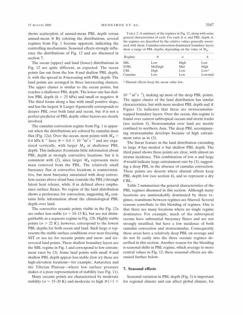
shows scatterplots of annual-mean PBL depth versusannual-mean B. By coloring the distributions, severalregimes from Fig. 1 become apparent, indicating thecontrolling mechanisms. Seasonal effects strongly influ-ence the distributions of Fig. 12 and are discussed insection 7.

The ocean (upper) and land (lower) distributions inFig. 12 are quite different, as expected. The oceanpoints fan out from the low B and shallow PBL depth,h, with the spread in B increasing with PBL depth. Theland points are arranged in three intersecting clusters.The upper cluster is similar to the ocean points, butreaches a shallower PBL depth. The lower one has shal-low PBL depth (h � 25 hPa) and small or negative B.The third forms along a line with small positive slope,and has the largest B. Larger B generally corresponds todeeper PBL over both land and ocean, but B is not aperfect predictor of PBL depth; other factors are clearlyinvolved.

The cumulus convection regime from Fig. 1 is appar-ent when the distributions are colored by cumulus massflux (Fig. 12a). Over the ocean, most points with MB �0.4 hPa h�1 have B � 0.4 � 10�3m2 s�3 and are orga-nized vertically, with larger MB at shallower PBLdepth. This indicates B contains little information aboutPBL depth at strongly convective locations, but it isconsistent with (2), since larger MB represents moremass removed from the PBL. The relatively smallbuoyancy flux at convective locations is counterintui-tive, but most buoyancy associated with deep convec-tion occurs above cloud base (outside the PBL) throughlatent heat release, while B as defined above empha-sizes surface fluxes. No region of the land distributionshows a preference for convection, suggesting MB con-tains little information about the climatological PBLdepth over land.

The convective oceanic points visible in the Fig. 12aare rather less stable (� � 10–13 K), but are not distin-guishable as a separate regime in Fig. 12b. Highly stablepoints (� � 22 K), however, correspond to the lowestPBL depths for both ocean and land. Such large � rep-resents the stable surface conditions over near-freezingSST or sea ice for oceanic points and snow- and ice-covered land points. These shallow boundary layers arethe SBL regime in Fig. 1 and correspond to low entrain-ment rates by (3). Some land points with small B andshallow PBL depth appear less stable (low �); these arehigh-elevation locations—for example, Antarctica andthe Tibetan Plateau—where low surface pressuremakes � a poor representation of stability (see Fig. 11).

Many oceanic points are characterized by moderatestability (� � 15–20 K) and moderate to high B (�1 �

10�3 m2 s�3), making up most of the deep PBL points.The upper cluster of the land distribution has similarcharacteristics, but with more modest PBL depth and B.Figure 12c indicates that these are stratocumulus-topped boundary layers. Over the ocean, this regime isfound over eastern subtropical oceans and storm tracks(see section 3). Stratocumulus over land are mostlyconfined to northern Asia. The deep PBL accompany-ing stratocumulus develops because of high entrain-ment rates as in (3).

The linear feature in the land distribution extendingto large B has modest � but shallow PBL depth. Thethird panel shows these points are clear, with almost nostratus incidence. This combination of low � and largeB would indicate large entrainment rate by (3), suggest-ing a deep PBL in the absence of cumulus convection.These points are deserts where diurnal effects keepPBL depth low (see section 4), and so represent a dryCBL.

Table 2 summarizes the general characteristics of thePBL regimes discussed in this section. Although manylocations are unmistakably dominated by these re-gimes, transitions between regimes are blurred. Severalreasons contribute to this blending of regimes. One isthat there are many locations where no single regimedominates. For example, much of the subtropicaloceans have substantial buoyancy fluxes and are notstrongly stratified, but have a low incidence of bothcumulus convection and stratocumulus. Consequentlythese areas have a relatively deep PBL on average anddo not fit easily into the three oceanic regimes de-scribed in this section. Another reason for the blendingis seasonal shifts in PBL regime, which average to morecentral values in Fig. 12; these seasonal effects are dis-cussed further below.

7. Seasonal effects

Seasonal variation in PBL depth (Fig. 3) is importantfor regional climate and can affect global climate, for

TABLE 2. A summary of the regimes in Fig. 12, along with somegeneral characteristics of each. For each B, �, and PBL depth, h,the regimes are described by the relative values generally associ-ated with them. Cumulus-convection-dominated boundary layersshow a range of PBL depths, depending on the value of MB.

Regime B � h

SBL Low High LowSTBL Mid/high Mid HighCBL High Low Low*Cumulus Low Low Low/mid

* Diurnal effects keep the mean value low.


example, by influencing seasonal deep convection orlow-level cloudiness. This section examines seasonalvariations in PBL depth using the concepts from above.

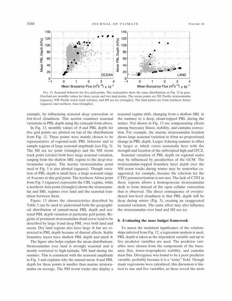
In Fig. 13, monthly values of B and PBL depth forfive grid points are plotted on top of the distributionsfrom Fig. 12. These points were mainly chosen to berepresentative of regional-scale PBL behavior and tosample regions of large seasonal amplitude (see Fig. 3).The SH sea ice point (triangles) and the NH stormtrack point (circles) both have large seasonal variation,ranging from the shallow SBL regime to the deep stra-tocumulus regime. The marine stratocumulus pointused in Fig. 5 is also plotted (squares). Though varia-tion of PBL depth is small here, a large seasonal rangeof B occurs at this grid point. The northern Africa pointfrom Fig. 5 (squares) represents the CBL regime, whilea northern Asia point (triangles) shows the stratocumu-lus and SBL regimes over land and the seasonal tran-sition between them.

Figure 13 shows the characteristics described byTable 2 can be used to understand both the geographi-cal distribution of annual-mean PBL depth and sea-sonal PBL depth variation at particular grid points. Re-gions of persistent stratocumulus cloud cover tend to bedescribed by large B and deep PBL over both land andocean. Dry land regions also have large B, but are re-stricted in PBL depth because of diurnal effects. Stableboundary layers have shallow PBL depth and small B.

The figure also helps explain the mean distributions.Stratocumulus over land is strongly seasonal and ismostly restricted to high-latitude, NH land during thesummer. This is consistent with the seasonal amplitudein Fig. 3 and explains why the annual-mean B and PBLdepth for these points is smaller than marine stratocu-mulus on average. The NH storm tracks also display a

seasonal regime shift, changing from a shallow SBL inthe summer to a deep, cloud-topped PBL during thewinter. Not shown in Fig. 13 are compensating effectsamong buoyancy fluxes, stability, and cumulus convec-tion. For example, the marine stratocumulus locationshows large seasonal variation in B but no proportionalchange in PBL depth. Larger B during summer is offsetby larger �, which varies seasonally here with thestrength and location of the subtropical high and ITCZ.

Seasonal variation of PBL depth on regional scalesmay be influenced by peculiarities of the GCM. Thestratocumulus-topped boundary layer depth over theNH storm tracks during winter may be somewhat ex-aggerated, for example, because the criterion for theCTEI parameterization is not met. The lack of CTEI inthese regions allows a homogeneous stratocumulusdeck to form instead of the open cellular convectionthat is observed. The direct consequence of overpre-dicted low-level cloudiness is that PBL depth will bedeep during winter (Fig. 3), creating an exaggeratedseasonal variation. The same effect may also influencethe stratocumulus over land and SH sea ice.

8. Evaluating the mass budget framework

To assess the statistical significance of the relation-ships inferred from Fig. 12, a regression analysis is used.PBL depth is taken as the dependent variable and up tofive predictor variables are used. The predictor vari-ables were chosen from the components of the buoy-ancy flux, lower-tropospheric stability, and cumulusmass flux. Divergence was found to be a poor predictorvariable, probably because it is a “noisy” field. Thoughmany regressions were calculated, this discussion is lim-ited to one and five variables, as these reveal the most

FIG. 13. Seasonal behavior for five grid points. The scatterplots show the same distributions as Fig. 12 in gray.Overlaid are monthly values for three ocean and two land points. The ocean points are NE Pacific stratocumulus(squares), NW Pacific storm track (circles), and SH sea ice (triangles). The land points are from northern Africa(squares) and northern Asia (triangles).


important physical insights. Because of the differencein PBL behavior over land and ocean, they are dis-cussed separately.

Correlations between predictor variables and PBLdepth showed differences between the land and oceanpoints. Lower-tropospheric stability, �, is the best pre-dictor over the ocean, while buoyancy flux due tocloud-top cooling, BR, does the best over land. Lower-tropospheric stability is anticorrelated with PBL depthand accounts for 65% of the variability for the oceanpoints while BR accounts for 66% of the variability inPBL depth over land.

For both land and ocean, the best predictor variables(BR and �, respectively) are variables that can discrimi-nate between clear and cloudy boundary layers. Thefact that the best predictor is different between landand ocean gives some sense that there is a fundamentaldifference arising from the land–sea contrast discussedin section 4. Lower-tropospheric stability explainsmuch of the oceanic variability by differentiating be-tween the less stable low latitudes and the highly stablehigh latitudes, and it contains information about re-gional-scale variability associated with cloud-toppedPBL regimes. Over land, BR is the best predictor be-cause it discriminates clear and cloudy boundary layers.It is a better predictor than � over land because diurnaland topographic effects erode the effectiveness of � incapturing PBL depth variability over land.

Using all five variables (BH,E,R, �, and MB) accountsfor 83% of PBL depth variability over land, and almost91% of the variability over ocean. The resulting esti-mates for PBL depth are given by

ho � 60.27 � 6005BH � 1.424 � 105BE � 32130BR

� 1.830� � 12.58MB, �5�

hl � 12.72 � 4434BH � 43990BE � 56003BR

� 0.0425� � 2.207MB. �6�

The much larger regression constant for ocean (60 ver-sus 12) suggests the larger oceanic mean PBL depth. Inboth expressions, the BH coefficient is much smallerthan the other buoyancy contributions, showing therelative insignificance of sensible heat flux anomaliesfor mean PBL depth. In both expressions the otherbuoyancy flux coefficients are positive, with BE espe-cially dominant over ocean and BR largest over land.Ocean points are most sensitive to BE because changesin latent heat flux are most likely to correspond with achange in PBL regime, while over land BR more suc-cessfully indicates changes between regimes. The � co-efficient is opposite signed for ocean and land. Oceanlocations have a strong anticorrelation between PBL

depth and �, as discussed above, while � is nearly neg-ligible over land. Cumulus mass flux reduces PBLdepth everywhere, but is more predictive for ocean, asinferred from Fig. 12. These results show the mass bud-get framework is appropriate for understanding themean behavior of the PBL.

9. Summary and conclusions

This paper seeks an understanding of the large-scalespatial structure of climatological PBL depth, includingseasonal and diurnal variations. The analysis uses theUCLA atmospheric GCM, a simple convective bound-ary layer model, and the PBL mass budget to show thePBL is organized into a few regimes and the depth iscontrolled largely by a few parameters. The most com-mon regimes are stratocumulus-topped boundary lay-ers, dry convective boundary layers, stable boundarylayers, and shallow boundary layers under the influenceof deep convection. Some general characteristics ofthese regimes are listed in Table 2 and are representedschematically in Fig. 1. The global perspective pre-sented here anticipates global PBL datasets providingsufficient information for a similar analysis, whichcould be useful in understanding the PBL and its role inclimate as well as comparison with climate models.

Great effort was devoted to parameterizing the PBLin the UCLA atmospheric GCM, with special caregiven to the treatment of boundary layer clouds. Therepresentation of stable boundary layers, however, suf-fers somewhat under the assumptions used. Relying ona CTEI assumption may also have an impact on meanPBL depth by overpredicting seasonal cloud cover overland and storm tracks. Despite these deficiencies, themixed-layer framework compares favorably againstother PBL schemes (Ayotte et al. 1996).

Figure 2 shows a strong land–sea contrast in annual-mean PBL depth, with much shallower PBL over land.A GCM simulation excluding diurnal variation in sun-shine showed much less difference between land andocean (Fig. 6). A CBL model also shows an increase inmean PBL depth without the diurnal cycle. In this CBLmodel the nightly PBL collapse reduces mean PBLdepth and creates a residual layer above the PBL. Theresidual layer acts as a heat reserve for the PBL, allow-ing its heat budget to control both daily maximum PBLdepth and the fraction of the day with a deep PBL.These effects are strong over land, where surface ther-mal conductivity is small, but the ocean feels much lessdiurnal variation. This leads to the land–sea contrastapparent in Fig. 2. The diurnal variation of PBL depthhas important implications for surface–atmosphere ex-change (see also Denning et al. 1996), and its represen-tation may be necessary for many applications.


The PBL mass budget, (1), decomposes the processesaffecting PBL depth, and the steady-state solution, (2),gives an approximate expression for PBL depth. Lo-cally generated buoyancy fluxes and lower-tropospher-ic stability account for most of the spatial variability inannual-mean PBL depth. These are related to the en-trainment rate by (3), and PBL depth scales as the en-trainment rate. Cumulus mass flux can also play animportant role in PBL depth over the tropical ocean.Figure 12 captures much of the large-scale organizationof PBL depth, clearly showing the most prevalent PBLregimes and the difference between land and ocean.Regression analysis shows the mass budget approachsuccessfully accounts for most PBL depth variability onlarge scales, and indicates the relative importance ofthe mass budget terms. The majority of the variability isaccounted for by only a few predictor variables. Such anestimation may be useful in the development of simpli-fied climate models in which detailed PBL schemes arean impediment.

Acknowledgments. This work was supported by NSFGrants ATM-0135136 and ATM-9985413.

APPENDIX

A Simple CBL Model

The formulation of the simple CBL model is similarto Tennekes (1973) and Carson (1973). To start, anenvironmental temperature profile, �(z) � �ref � �h, isprescribed, where � is potential temperature, �ref a ref-erence temperature, � a stability, and h the PBL depth.This is solved for h once �(z) is determined. When awell-mixed assumption is included, the vertical depen-dence vanishes. The PBL’s potential temperature is de-termined by surface heat fluxes. To obtain the heat flux,a surface energy balance is used to establish the groundtemperature, Tg,

cpg

dTg

dt� S � �Tg

4 � F, �A1�

where cpg is the surface isobaric specific heat, S is in-coming radiative flux, �T 4

g is outgoing blackbody radia-tion, and F is surface heat flux.

For experiments with a diurnal cycle, the incomingradiation is a clipped sine wave,

S � �S� sin�2�t

�� if sin�2�t

�� 0

0 if sin�2�t

�� 0

, �A2�

where S� is the solar flux and �� (� 86 400 s�1) is therotation frequency of earth. When the diurnal cycle is

removed, S is set to its mean from the time-varyingexperiment.

Sensible heat flux is determined from a bulk aero-dynamic formula, F � cpd�CD||V ||(Tg � �), where CD

(� 0.0011) and ||V || is a prescribed mean wind speed.The mixed-layer potential temperature is used since itis identical to the surface air temperature by construc-tion.

The evolution of the potential temperature is takenas the change in vertical heat flux [�t� � ��z(w�)].Integrating across the PBL, and assuming the heat fluxat the CBL top is 20% of the surface value ��(w�)h �0.2(w�)0] gives an expression for potential tempera-ture, �t� � 1.2(w�)0h�1.

The surface heat flux is transformed between kine-matic and energetic units by cpd�(w�)0 � F. This givesan equation for the potential temperature in terms of Fand h[�t� � 1.2F(cpd�h)�1] and closes this model.

To model the diurnal variation in PBL height, it isnecessary to allow a rapid collapse of the PBL. Thecollapse is due a surface inversion forming when theground cools, decoupling the surface fluxes from thedaytime mixed layer. In keeping with the simplicity ofthe current framework, a switching rule determines thecollapse of the PBL,

h � ��ML � �ref

�H�F � � hminH��F �, �A3�

where H denotes the Heaviside function, and hmin is aminimum PBL height representing mechanically driventurbulence (usually set to 100 m). To avoid instanta-neous mixing of residual-layer air, and maintain a con-sistent heat budget, the residual layer is explicitly in-cluded. This layer is considered well mixed in �, whoseinitial value is determined by the deep daytime PBL. Arelaxation parameter, �, represents the time it takes forthe residual layer to cool to the free tropospheric lapserate,

d�r

dt� ��ML � �ref

�. �A4�

In this case, �ML is the larger of the mixed-layer orresidual-layer potential temperature.

Without (A3) the model cannot reproduce the dailycycle of PBL depth (Fig. 5), but it complicates the heatbudget. Equation (A4) is a parameterization of diabaticprocesses that fits with our simple approach to theproblem, and it successfully balances the heat budget.

The choice of � accounts for radiative cooling andmixing in the residual layer, so depends on factors nottaken into account by this CBL model. A test of thesensitivity of the CBL model to this time scale is shownin Fig. A1. As � increases, the mean and maximum daily


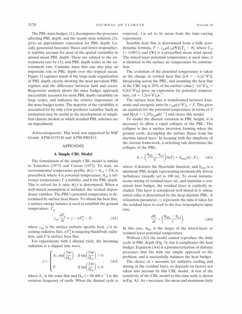
PBL depth increase parabolically as less heat acquiredby the residual layer from the PBL is lost during thenight. Daily maximum PBL depth is somewhat moresensitive to changes in the relaxation time scale thanmean PBL depth. This follows the reasoning given insection 4.

REFERENCES

Albrecht, B. A., C. S. Bretherton, D. Johnson, W. S. Schubert,and A. S. Frisch, 1995: The Atlantic stratocumulus transitionexperiment—ASTEX. Bull. Amer. Meteor. Soc., 76, 889–904.

Arakawa, A., and W. H. Schubert, 1974: Interaction of a cumuluscloud ensemble with the large-scale environment, Part I. J.Atmos. Sci., 31, 674–701.

Avissar, R., and C. Nobre, 2002: Preface to special issue on theLarge-Scale Biosphere–Atmosphere Experiment in Amazonia(LBA). J. Geophys. Res., 107, 8034, doi:10.1029/2002JD002507.

Ayotte, K. W., and Coauthors, 1996: An evaluation of neutral andconvective planetary boundary-layer parameterizations rela-tive to large eddy simulations. Bound.-Layer Meteor., 79,131–175.

Barr, A. G., and A. K. Betts, 1997: Radiosonde boundary layerbudgets above a boreal forest. J. Geophys. Res., 102 (D24),29 205–29 212.

Betts, A. K., J. H. Ball, A. C. M. Beljaars, M. J. Miller, and P. A.Viterbo, 1996: The land surface–atmosphere interaction: Areview based on observational and global modeling perspec-tives. J. Geophys. Res., 101 (D3), 7209–7225.

Bretherton, C. S., and Coauthors, 2004: The EPIC 2001 stratocu-mulus study. Bull. Amer. Meteor. Soc., 85, 967–977

Carson, D., 1973: The development of a dry inversion-cappedconvectively unstable boundary layer. Quart. J. Roy. Meteor.Soc., 99, 450–467.

Deardorff, J. W., 1972: Parameterization of the planetary bound-ary layer for use in general circulation models. Mon. Wea.Rev., 100, 93–106.

——, 1980: Cloud top entrainment instability. J. Atmos. Sci., 37,131–147.

Denning, A. S., D. A. Randall, G. J. Collatz, and P. J. Sellers,1996: Simulations of terrestrial carbon metabolism and atmo-spheric CO2 in a general circulation model: Part 2: SimulatedCO2 concentrations. Tellus, 48B, 543–567.

Garratt, J., L. Rotstayn, and P. Krummel, 2002: The atmosphericboundary layer in the CSIRO global climate model: Simula-tions versus observations. Climate Dyn., 19, 397–415.

Klein, S. A., and D. L. Hartmann, 1993: The seasonal cycle of lowstratiform clouds. J. Climate, 6, 1587–1606.

LeMone, M. A., and Coauthors, 2000: Land–atmosphere interac-tion research, early results, and opportunities in the WalnutRiver Watershed in southeast Kansas: CASES and ABLE.Bull. Amer. Meteor. Soc., 81, 757–779.

Lenschow, D. H., and Coauthors, 1988: Dynamics and chemistryof marine stratocumulus (DYCOMS) experiment. Bull.Amer. Meteor. Soc., 69, 1058–1067.

Lewellen, D., and W. Lewellen, 1998: Large-eddy boundary layerentrainment. J. Atmos. Sci., 55, 2645–2665.

Li, J.-L. F., and A. Arakawa, 1999: Improved simulation of PBLmoist processes with the UCLA GCM. Preprints, SeventhConf. on Climate Variation, Long Beach, CA, Amer. Meteor.Soc., 35–40.

——, M. Köhler, J. D. Farrara, and C. Mechoso, 2002: The impactof stratocumulus cloud radiative properties on surface heatfluxes simulated with a general circulation model. Mon. Wea.Rev., 130, 1433–1441.

Lilly, D. K., 1968: Models of cloud topped mixed layers under astrong inversion. Quart. J. Roy. Meteor. Soc., 94, 292–309.

Lock, A., A. Brown, M. Bush, G. Martin, and R. Smith, 2000: Anew boundary layer mixing scheme. Part I: Scheme descrip-tion and single-column model tests. Mon. Wea. Rev., 128,3187–3199.

Martin, G., M. Bush, A. Brown, A. Lock, and R. Smith, 2000: Anew boundary layer mixing scheme. Part II: Tests in climateand mesoscale models. Mon. Wea. Rev., 128, 3200–3217.

McCormick, M. P., and Coauthors, 1993: Scientific investigationsplanned for the Lidar In-space Technology Experiment(LITE). Bull. Amer. Meteor. Soc., 74, 205–214.

Mechoso, C. R., J.-Y. Yu, and A. Arakawa, 2000: A coupledGCM pilgrimage: From climate catastrophe to ENSO simu-lations. General Circulation Model Development: Past,Present, and Future, D. A. Randall, Ed., Academic Press,539–575.

Moeng, C.-H., and B. Stevens, 2000: Marine stratocumulus and itsrepresentation in GCMs. General Circulation Model Devel-opment: Past, Present, and Future, D. A. Randall, Ed., Aca-demic Press, 577–604.

Neiburger, M., D. S. Johnson, and C.-W. Chien, 1961: Studies ofthe structure of the atmosphere over the eastern Pacificocean in summer. University of California Tech. Rep., 94 pp.

Randall, D. A., 1980: Entrainment into a stratocumulus layer withdistributed radiative cooling. J. Atmos. Sci., 37, 148–159.

——, J. A. Abeles, and T. G. Corsetti, 1985: Seasonal simulationsof the planetary boundary layer and boundary-layer stratocu-mulus clouds with a general circulation model. J. Atmos. Sci.,42, 641–676.

——, Q. Shao, and M. Branson, 1998: Representation of clear andcloudy boundary layers in climate models. Clear and CloudyBoundary Layers, A. A. M. Holtslag and P. G. Duynkerke,Eds., Royal Netherlands Academy of Arts and Sciences, 305–322.

FIG. A1. Sensitivity of mean and maximum PBL height (m) toresidual-layer relaxation time scale, � (h). The solid line is themean PBL top height from the CBL model, and the dashed line isthe peak height. Experiments were run with � equal to 1, 6, 10, andmultiples of 6 up to 120 h.


Sellers, P. J., F. G. Hall, G. Asrar, D. E. Strebel, and R. E. Mur-phy, 1992: An overview of the First ISLSCP Field Experi-ment. J. Geophys. Res., 97 (D17), 18 345–18 372.

——, and Coauthors, 1995: The Boreal Ecosystem–AtmosphereStudy (BOREAS): An overview and early results from the1994 field year. Bull. Amer. Meteor. Soc., 76, 1549–1577.

Stage, S. A., and J. A. Businger, 1981: A model for entrainmentinto a cloud-topped marine boundary layer. Part I: Modeldescription and application to a cold-air outbreak episode. J.Atmos. Sci., 38, 2213–2229.

Stevens, B., 2002: Entrainment in stratocumulus-topped mixedlayers. Quart. J. Roy. Meteor. Soc., 128, 2663–2690.

——, and Coauthors, 2003: Dynamics and chemistry of marinestratocumulus—DYCOMS-II. Bull. Amer. Meteor. Soc., 84,579–593.

Stull, R. B., 1988: Introduction to Boundary Layer Meteorology.Kluwer Academic, 666 pp.

Suarez, M., A. Arakawa, and D. Randall, 1983: The parameter-ization of the planetary boundary layer in the UCLA generalcirculation model: Formulation and results. Mon. Wea. Rev.,111, 2224–2243.

Tennekes, H., 1973: A model for the dynamics of the inversionabove a convective boundary layer. J. Atmos. Sci., 30, 558–567.

Uttal, T., and Coauthors, 2002: Surface heat budget of the ArcticOcean. Bull. Amer. Meteor. Soc., 83, 255–276.

Webster, P. J., and R. Lukas, 1992: TOGA COARE: TheCoupled Ocean–Atmosphere Response Experiment. Bull.Amer. Meteor. Soc., 73, 1377–1416.

Winker, D. H., R. H. Couch, and M. P. McCormick, 1996: Anoverview of LITE: NASA’s Lidar In-space Technology Ex-periment. Proc. IEEE, 84 (2), 1–17.

Yanai, M., and C. Li, 1994: Mechanism of heating and the bound-ary layer over the Tibetan Plateau. Mon. Wea. Rev., 122,305–323.


what controls the mean depth of the pbl? - ucla ... controls the mean depth of the pbl? brian...

Documents