weno scheme with subcell resolution for computing ...scholarism.net/fulltext/ijmcs20154004.pdf ·...

International Journal of Mathematics and Computer Sciences (IJMCS) ISSN: 2305-7661 Volume.40 2015 www.scholarism.net

1301

WENO Scheme with Subcell Resolution for Computing Nonconservative Euler

Equations with Applications to One-Dimensional Compressible Two-Medium Flows

1 Tao Xiong

, 2 Chi-Wang Shu

1 School of Mathematical Sciences, University of Science and Technology of China, Hefei, Anhui, China

2 Division of Applied Mathematics, Brown University, Providence

Abstract

High order path-conservative schemes have been developed for solving nonconservative hyperbolic systems in

(Parés, SIAM J. Numer. Anal. 44:300–321, 2006; Castro et al., Math. Comput. 75:1103–1134, 2006; J. Sci.

Comput. 39:67–114, 2009). Recently, it has been observed in (Abgrall and Karni, J. Comput. Phys. 229:2759–

2763, 2010) that this approach may have some computational issues and shortcomings. In this paper, a

modification to the high order path-conservative scheme in (Castro et al., Math. Comput. 75:1103–1134, 2006)

is proposed to improve its computational performance and to overcome some of the shortcomings. This

modification is based on the high order finite volume WENO scheme with subcell resolution and it uses an

exact Riemann solver to catch the right paths at the discontinuities. An application to one-dimensional

compressible two-medium flows of nonconservative or primitive Euler equations is carried out to show the

effectiveness of this new approach.

Keywords

Path-conservative schemes High order finite volume WENO scheme Subcell resolution Nonconservative

hyperbolic systems Primitive Euler equations Two-medium flows Exact Riemann solver

Dedicated to Professor Saul Abarbanel on the occasion of his 80th birthday.

C.-W. Shu was supported by ARO grant W911NF-11-1-0091 and NSF grant DMS-1112700.

M. Zhang was supported by NSFC grant 11071234.

Introduction

Recent years have seen a growing interest in developing numerical algorithms for solving compressible

multicomponent flows. The dynamics of inviscid multicomponent fluid may be modeled by the Euler equations.

However, computations often run into unexpected difficulties due to nonphysical oscillations generated at the

vicinity of the material interface, while such oscillations do not arise in single-fluid computations when a

nonlinearly stable scheme, such as the essentially non-oscillatory (ENO) or weighted ENO (WENO) scheme

[18, 22, 32, 41], is used. The underlying mechanisms have been analyzed and several methods have been

developed to overcome these difficulties, e.g. in [1, 2, 5, 10, 24, 25, 28].

There are mainly two approaches to circumvent these oscillations. One is still based on the conservative Euler

equations, and the other is to write the Euler equations in nonconservative or primitive form.

The ghost fluid method (GFM) developed in [14] with the isobaric fix technique in [15] has provided an

attractive and flexible way to treat the two-medium flow model for conservative Euler equations. The GFM

treats the material interface as an internal boundary, and by defining ghost cells and ghost fluids, the two-

medium flow can be solved via two respective single-medium Riemann problems. This method is simple, can be

easily extended to multi-dimensions, and can maintain a sharp interface without oscillations. Variants of the

original GFM and their applications can be found in, e.g. [28–30, 30] and the references therein. Later, these

techniques are used to develop the Runge-Kutta discontinuous Galerkin (RKDG) finite element method for

multi-medium flow in [36, 37, 29, 33]. The GFM, even though approximating directly the conservative Euler

equations, is in general not a conservative method because the flux at the interface is double-valued. Recently, a

conservative modification to the GFM using the fifth order finite difference WENO scheme with third order

http://link.springer.com/article/10.1007/s10915-012-9578-7/fulltext.html#ContactOfAuthor2

http://link.springer.com/article/10.1007/s10915-012-9578-7/fulltext.html#CR35


























1302

Runge-Kutta time discretization has been studied in [31], which attempts to reduce the conservation error of the

GFM without affecting its performance.

The other approach is based on the observation that erroneous pressure fluctuations are generated by the

conservative equations, hence a better approximation can be obtained when writing the equations in a

nonconservative (primitive) form [23, 24]. In these papers a scheme for the nonconservative Euler formulation

is proposed, with consistent correction terms to remove the leading order conservation errors. This scheme can

completely eliminate spurious oscillations at the material interface, yielding clean monotonic solution profiles.

This work has been extended to solve two dimensional problems in [38]. In this method, the correction terms

depend heavily on the corresponding conservative numerical scheme. Only second order nonconservative

schemes are considered and they are only applied to shocks of weak to moderate strengths. This method is also

less justifiable for high-resolution schemes with narrow shock transition and it is not justified in cases of strong

shocks [20]. It is noted in these papers that, for nonconservative hyperbolic systems, the shock relationships are

not uniquely defined by the limiting left and right states, as they also depend on the viscous path connecting the

two states. The correct shock capturing lies in getting correctly the viscous path.

The theory developed by Dal Maso, LeFloch and Murat [12] gives a rigorous definition of nonconservative

products, associated with the choice of a family of paths. Later, people have paid much attention to the

development of numerical schemes for solving nonconservative hyperbolic systems, see for example [6–8,35]

and references therein. A high order Roe-type scheme based on the reconstructed states has been provided in [7]

for the one-dimensional case, and then extended to two dimensions in [6], but only with applications to shallow-

water systems. Other work based on this high order method has been carried out for solving two-phase flow

models in [13, 24, 26]. A limitation of this approach has been pointed out recently in [3] when applied to

nonconservative Euler equations. The problem is related to the effective choice of a correct path in the

nonconservative high order scheme. It appears that, for nonconservative Euler equations, using the Roe

linearization to choose a path as in [6, 7, 28] might end up in converging to a weak solution of a different path

[3], see also this deficiency in Fig. 3 of our Example 3 in Sect. 8. Several natural questions were raised in [3] for

the path-conservative schemes, including (i) how does one go about choosing a path; (ii) what influence does

the choice of path and discretization scheme have on the computed solution; (iii) once a path is specified and a

consistent path-conservative scheme designed, does the numerical solution converge to the assumed path; and

(iv) in cases where the correct jump conditions are known unambiguously, can a path-conservative scheme be

designed so that it converges to the correct solution. The answer to (i) is likely to have to come from physics.

For a non-conservative formulation of a conservative system, as is the case discussed in this paper, the choice of

the path can be achieved by an exact Riemann solver. We attempt to discuss possible approaches to address (ii),

(iii) and (iv) in this paper. We focus on adapting high order schemes for solving nonconservative Euler

equations, still based on high order Roe-type finite volume schemes as those in [6, 7]. For the nonconservative

or primitive Euler equations, the right path should recover the weak solution of the conservative Euler

formulation with density, momentum and energy as its variables. In smooth regions, the conservative and

nonconservative Euler equations are equivalent, but at discontinuities, they are not [23]. As is well known,

shock capturing schemes such as monotone, total variation diminishing (TVD), or ENO and WENO schemes,

smear discontinuities with one or several transitional points. These transitional points are necessary for

conservation, however in a nonconservative formulation, they may not land on the correct path in the phase

space and hence may lead to convergence to erroneous weak solutions on different paths. Realizing this

difficulty, which unfortunately is generic with all shock capturing schemes, our basic idea in this paper is to use

Harten’s subcell resolution technique [17] to sharpen the discontinuities and effectively eliminate (or at least

significantly reduce) the transitional points. As a result, the convergence towards the correct weak solution

based on the originally desired path seems to be restored.

Harten’s subcell resolution idea [17] is based on ENO schemes with a Lax-Wendroff time discretization

procedure in a cell-averaged framework. Later, this idea is extended in [42] to both finite volume and finite

difference ENO schemes with Runge-Kutta time discretization. Recently, this subcell resolution idea has been

used in solving advection equations with stiff source terms, to obtain correct shock speed on coarse meshes [31].

In this paper, with the sharp left and right states at the discontinuities, we use an exact Riemann solution to catch

the right path that connects the two states, as the correct capturing of the shock speed is sensitive to the accuracy

of the numerically achieved path. Numerical experiments for one-dimensional compressible one- and two-

medium flows of nonconservative Euler equations show the effectiveness of our new approach. Based on these

results, we give partial answers to the questions in [3] as quoted above: (i) at least for nonconservative or

primitive Euler equations, the right path should recover the weak solution of the conservative Euler formulation

with density, momentum and energy as its variables; (ii) at least for non-conservative Euler equations, different

paths would lead to very different weak solutions; (iii) numerical solution from a path-conservative scheme

designed for a specified path, with a smeared shock front, does not necessarily converge to the weak solution

corresponding to the desired path, see for example Fig. 3 in Sect. 8; (iv) at least for the nonconservative Euler

equations, where we know the correct jump conditions, our approach of high order Roe path-conservative




















http://link.springer.com/article/10.1007/s10915-012-9578-7/fulltext.html#Fig3

http://link.springer.com/article/10.1007/s10915-012-9578-7/fulltext.html#Sec11













1303

scheme with subcell resolution can effectively remove smearing of discontinuities, leading to convergence to the

correct solution.

This paper is organized with the following sections. In Sect. 2, we first describe the high order Roe scheme for

the nonconservative hyperbolic systems. Then we introduce the two-medium flow model for nonconservative

Euler equations in Sect. 3. In Sect. 4, we illustrate how to apply the WENO reconstruction with subcell

resolution to the high order Roe scheme. In Sect. 5, we describe the computation of the integral term in the high

order Roe scheme in detail. In Sect. 6, we present the level set function to track the material interface.

A summary of our algorithm to aid implementation is given in Sect. 7, and one-dimensional numerical examples

are provided to demonstrate the effectiveness of our approach in Sect. 8. Concluding remarks follow in the last

section.

High Order

Roe Scheme for Nonconservative Hyperbolic Systems

In this section, we follow the procedure in [7] to define the high order Roe scheme for solving nonconservative

hyperbolic systems. For the one-dimensional case, a nonconservative hyperbolic system reads

Wt+A(W)Wx=0,x∈Ω⊂R, t>0

(2.1)

where W=W(x,t) is a N-component state vector and A(W) is a N×N matrix. The system is supposed to be

hyperbolic, i.e. A(W) has N real eigenvalues and a full set of N linearly independent eigenvectors.

For simplicity, we use a uniform grid

$$a = x_{\frac{1}{2}} < x_{\frac{3}{2}} < \cdots< x_{N_x-\frac{1}{2}}<="" div="" style="outline: 0px;">

The cells, cell centers, and the uniform cell size are denoted by

Ii≡[xi−12,xi+12],xi≡12(xi−12+xi+12),Δx≡xi+12−xi−12,i=1,2,…,Nx.

In the case of systems of conservation laws, that is when A(W)=∂F/∂W, which is the Jacobian of a flux

function F(W), (2.1) reduces to a classical conservation law

Wt+F(W)x=0.

(2.2)

A conservative finite volume semi-discretization [26] of the system (2.2) is

W′i(t)=1Δx(Gi−1/2−Gi+1/2),

(2.3)

with the numerical flux

Gi+1/2=G(W−i+1/2(t),W+i+1/2(t)),

(2.4)

where W i (t) is used to approximate the cell averaged value W¯¯¯¯i(t), which is defined as

W¯¯¯¯i(t)=1Δx∫xi+1/2xi−1/2W(x,t)dx,

and W±i+1/2(t) are the left and right limits of solutions at the cell boundary x i+1/2, which are the reconstructed

states associated to the cell average sequence {W j (t)}.

The semi-discrete high order Roe scheme for (2.3) can be written as

(2.5)

which is equivalent to the conservative scheme (2.3) with the numerical flux (2.4) defined to be

(2.6)

Here

|Ai+1/2|=A+i+1/2−A−i+1/2









http://link.springer.com/article/10.1007/s10915-012-9578-7/fulltext.html#Equ1







1304

(2.7)

and the Roe property

Ai+1/2(W+i+1/2(t)−W−i+1/2(t))=F(W+i+1/2(t))−F(W−i+1/2(t))

(2.8)

has been used. The intermediate matrices are defined by

Ai+1/2=A^(W+i+1/2(t),W−i+1/2(t))

(2.9)

and

A±i+1/2=Ri+1/2Λ±i+1/2R−1i+1/2,Λ±i+1/2=diag((λ1)±i+1/2,…,(λN)±i+1/2)

(2.10)

where R i+1/2 is a N×N matrix with each column as a right eigenvector of A i+1/2, and Λ i+1/2 is the diagonal matrix

whose diagonal entries are the corresponding eigenvalues of A i+1/2. We have A^(W,W)=A(W), and a specific

definition of (2.9) is given in Sect. 4. In (2.10), we define

(x)+={x,0,if x>0otherwise(x)−={x,0,if x<0otherwise

so Λ±i+1/2 are the corresponding diagonal matrices with positive or negative eigenvalues.

We introduce Pti(x) as any smooth function defined in the cell I i , such that

limx→x+i−1/2Pti(x)=W+i−1/2(t),limx→x−i+1/2Pti(x)=W−i+1/2(t).

(2.11)

Then, (2.5) can be rewritten as

(2.12)

Now the numerical high order Roe scheme for solving the nonconservative system (2.1) can be easily

generalized from (2.12)

(2.13)

with the function Pti(x) satisfying (2.11). In order to obtain entropy-satisfying solutions, the Harten-Hyman

entropy fix technique [19, 47] can be applied to this scheme.

Two-Medium

Flow Model for Nonconservative Euler Equations

In this section, we describe the two-medium inviscid compressible flow model for the nonconservative or

primitive Euler equations. As pointed out in [23], the choice of the primitive set of variables, that include

density, velocity and pressure, provides a model better suited than the conserved variables for computations of

propagating material fronts. Such model results in clean and monotonic solution profiles, so we consider the

one-dimensional primitive Euler equations

Wt+A(W)Wx=0

(3.1)

with

(3.2)












1305

Here ρ is the density, u is the velocity, p is the pressure, γ is the ratio of specific heats. The total energy is given

by E=ρe+12ρu2, where e is the specific internal energy per unit mass. In Sect. 8, we will consider systems of

two gases and systems involving air and water. We will use the following γ-law equation of state (EOS) for both

air and water

ρe=p/(γ−1)

(3.3)

note that for the water medium, what we have actually used is the Tait EOS [9, 14, 28, 36], and we need to

use p¯=p+γB¯ instead of p in all the above formulae, where B¯=B−A, A=1.0E5 Pa and B=3.31E8 Pa. For

water, γ=7.15, and the displayed pressure for the water in Sect. 8 is p, not p¯.

WENO Reconstruction with Subcell Resolution

In this section, we will describe how to use the WENO reconstruction with subcell resolution to

reconstruct W±i+1/2(t) from the cell averages {W j (t)}. The WENO reconstruction is described in detail in

[22, 40]. We follow the procedure in [42] to describe how to apply the subcell resolution technique of Harten

[17] to the scheme (2.13) with the third order total variation diminishing (TVD) Runge-Kutta time discretization

[41], also called strong stability preserving (SSP) time discretization [16].

We first consider the 1D, scalar, linear version u t +f(u) x =0, with f(u)=au and a>0, to describe the WENO

reconstruction with the subcell resolution technique. The extension to the nonlinear and system cases will

follow. We would like to reconstruct u−i+1/2 and u+i−1/2 in each cell from the sequence of cell averages {u¯j},

with the following algorithm.

WENO Reconstruction Algorithm

Given the cell averages {u¯j} of a function u(x):

u¯j=1Δx∫xj+1/2xj−1/2u(ξ)dξ,j=1,2,…,Nx,

(4.1)

based on the big stencil S i ≡{I i−r ,…,I i ,…,I i+r }, a k-th (k=2r+1) order accurate approximation to the boundary

values u−i+1/2 and u+i−1/2 in the cell I i is reconstructed as

u−i+1/2=∑j=0rωj(xi+1/2)pj(xi+1/2),u+i−1/2=∑j=0rωj(xi−1/2)pj(xi−1/2)

(4.2)

where each p j (x) is a reconstruction polynomial that uses the cell averages in the small

stencil Sji≡{Ii−j,…,Ii−j+r}⊂Si. The nonlinear weights {ωj(x)}rj=0 are calculated from the

polynomials {pj(x)}rj=0 and the linear weights {dj(x)}rj=0 at each fixed point x, and they satisfy

ωj(x)>0,∑j=0rωj(x)=1.

(4.3)

The nonlinear weight ω j (x) is close to zero when a discontinuity is located in the stencil Sji, so as to avoid

involving much information from any stencil Sji which contains discontinuities.

Remark

For the cell boundaries (4.2), the linear weights d j (x i+1/2) and d j (x i−1/2) are positive. However, at certain

internal points x∈I i (reconstruction at those points are needed in Sect. 5), the linear weights d j (x) may be

negative. The linear weights may also become negative if the stencil S i is changed to S i+1 or S i−1, while still

reconstructing values in the cell I i (e.g. in the following subcell resolution algorithm). In these cases, the

technique to treat negative weights in [39] needs to be applied.

Subcell Resolution Algorithm

We describe the procedure for the three-stage third order TVD time discretization, specifically given as (7.1) in

Sect. 7. First, at the beginning of every Runge-Kutta stage:

(I) Define the “critical intervals” (intervals containing discontinuities) I i =(x i−1/2,x i+1/2) by σ i ≥σ i+1, σ i >σ i−1,

where σi=|m(Δ+u¯i,Δ−u¯i)|, Δ+u¯i=u¯i+1−u¯i, Δ−u¯i=u¯i−u¯i−1 and m is the minmod function which is

defined to be

m(a1,…,an)={smin1≤i≤n|ai|,0,if s=sign(a1)=⋯=sign(an)otherwise.

(4.4)

(II) For any “critical interval” I i , let θi=(u¯i+1−u¯i)/(u¯i+1−u¯i−1), and use x i−1/2+θ i Δx as an approximation

to the discontinuity location inside the cell I i .

Then, in each Runge-Kutta time stage, we perform:

(III) Let the cell I i boundary values u−i+1/2 and u+i−1/2 be defined as usual, using the standard WENO

reconstruction algorithm (4.2), unless I i or (for the second and third Runge-Kutta stages) I i−1 is a “critical

interval”. If I i is a “critical interval”, we define





















1306

(4.5)

(4.6)

where u−,oldi−1/2 is the standard WENO reconstruction with the stencil S i−1, u(L)i+1/2 is also the standard

WENO reconstruction with the stencil S i−1, but evaluated at x i+1/2 of the cell I i , and u(R)i+1/2 is the WENO

reconstruction with the stencil S i+1 and evaluated at x i+1/2. Notice that here for u(L)i+1/2 the technique for

treating negative weights needs to be used. For the second and third Runge-Kutta stages, we choose the

stencil S i+2 for u(R)i+1/2 if ξ i <1 and the negative weight treating technique needs to be used here as well.

When I i−1 is a “critical interval” and ξ i−1<1, we choose the stencil S i+1 for u−i+1/2.

Remark

(a) The case for a<0 is easily obtained by symmetry.

(b) For nonlinear systems, the subcell resolution algorithm is simply applied in each local characteristic field.

The detailed procedure can be found in [42]. The only difference in our current situation is that we just

useA(W i (t)) to do the characteristic decomposition when defining if I i is a “critical interval”. However if the

material interface is located in the cell I i , we always set it to be a “critical interval”, and we

use A(Wi(t)+Wi+1(t)2) to do the characteristic decomposition for the right cell boundary at x i+1/2,

and A(Wi−1(t)+Wi(t)2) for the left cell boundary at x i−1/2. The average to define the intermediate matrix in (2.9)

is

Ai+1/2=A^(W+i+1/2(t),W−i+1/2(t))=A(W+i+1/2(t)+W−i+1/2(t)2).

(c) For systems, due to different local characteristic decomposition, two adjacent cells might both be “critical

intervals”. In this situation, we remove the one with a smaller σ i from the list of critical intervals.

(d) It is pointed out in [17, 42] that the subcell resolution technique should be applied only to sharpen contact

discontinuities. Special caution is needed when one tries to sharpen a (nonlinear) shock, to avoid obtaining a

nonphysical, entropy condition violating solution. In our approach, the subcell resolution is used to get sharp left

and right states at the discontinuities. At a nonlinear shock, this is also needed so as to get a more accurate shock

speed which heavily depends on the left and right states. In the computation for Euler equations of compressible

gas dynamics, we apply the subcell resolution algorithm in both the linearly degenerate field and genuinely

nonlinear fields [26], but for the genuinely nonlinear fields, with eigenvalues λ Land λ R corresponding to the

left and right states respectively, we only apply the subcell resolution for the case λ L ≥λ R

to avoid sharpening a

rarefaction wave.

5 Choice of the Path and Evaluation of the Path Integral

In smooth regions, all simple wave models for conservative Euler equations and primitive Euler equations are

equivalent. However, near discontinuities, they are not equivalent [23]. According to this, our choice of the path

is divided into three parts: the smooth case, discontinuities in a single medium, and discontinuities at the

material interface.

5.1 The Smooth Case

In the smooth case, the integral term in (2.13)

∫xi+1/2xi−1/2A(Pti(x))ddxPti(x)dx

(5.1)

can be computed via a high order accurate Gauss-Lobatto quadrature rule. Given the positions {s j } and

associated weights {ω j } for a G-point quadrature in the interval [−12,12], we can replace the analytical path

integral (5.1) by

∫xi+1/2xi−1/2A(Pti(x))ddxPti(x)dx≈∑j=1GωjA(Pti(sj))ddxPti(sj).

(5.2)

In our numerical experiments, we use the four-point Gauss-Lobatto quadrature rule:

s1,4=∓12,s2,3=∓5√10,ω1,4=16,ω2,3=56.

(5.3)

For Pti(s1,4), from (2.11) we already have

Pti(s1)=W+i−1/2,Pti(s4)=W−i+1/2

(5.4)

following the same procedure for obtaining Pti(s1,4), we can also obtain Pti(s2,3), where Pti(s2) is obtained in

the same way as Pti(s1) corresponding to the local characteristic field at x i−1/2,











1307

and Pti(s3) as Pti(s4)corresponding to the local characteristic field at x i+1/2. Note here for the smooth case, we

do not need the subcell resolution in the WENO reconstruction. Since we have {Pti(sj)}4j=1, ddxPti(x) can be

approximated by Q(x), the derivative of the Lagrangian interpolation polynomial based on {Pti(sj)}4j=1.

Then ddxPti(sj) can be replaced by Q(s j ) in (5.2).

5.2 Discontinuities in a Single Medium

At the discontinuities, the cell is defined as a “critical interval”, and we have obtained the left and right

states W+i−1/2 and W−i+1/2 from the WENO reconstruction with subcell resolution in Sect. 4. Denote the left

and right states W+i−1/2 and W−i+1/2 to be W L and W R , we can use the exact Riemann solver [23, 26] to

obtain the exact Riemann solution between the two states. The exact Riemann solution for the compressible

Euler equations contains four constant states connected by a rarefaction wave or a shock wave, a contact

discontinuity, and another rarefaction wave or shock wave. The four constant states can be denoted

as W L ,W ∗L , W ∗R and W R . In this case of the “critical interval”, we use the exact Riemann solution to get the

integral path for the integral term (5.1). It can be computed as the following seven parts:

(a) The four constant-state parts, since ddxPti(x)=0, the integral in these four parts are all zero.

(b) If W L and W ∗L are connected by a rarefaction wave, we similarly use the 4-point Gauss-Lobatto quadrature

rule (5.3), and Pti(x) in this part is just the rarefaction wave line. Otherwise, if W L and W ∗L are connected by a

shock wave, then the integral path for this part needs to satisfy the Rankine-Hugoniot jump condition of the

conservative Euler equations, and the integral result is σ(W ∗L −W L ), with σ being the shock speed related to the

two states W L and W ∗L . Similar results can be obtained for the connection between W∗R and W R .

(c) For the contact discontinuity part between W ∗L and W ∗R , the integral path also needs to satisfy the Rankine-

Hugoniot jump condition. Since W ∗L and W ∗R have the same pressure p and velocity u and different

densities ρ ∗L and ρ ∗R , the integral result is simply (u(ρ ∗R −ρ ∗L ),0,0) T

.

Remark

In (b) and (c) above, for the shock wave and contact discontinuity, we do not need to know the exact integral

paths for satisfying the Rankine-Hugoniot jump condition, in order to get the integral results along those paths.

We only need to make sure that these paths exist, which can be easily verified.

5.3 Discontinuities at the Material Interface

We always set the cell at the material interface as a “critical interval”. The integral term (5.1) can be computed

similar to the second case of discontinuities in a single medium, as the exact Riemann solution at the material

interface is almost the same as that for the single-component compressible Euler equations, also containing four

constant states connected by a rarefaction wave or a shock wave, a contact discontinuity, and another rarefaction

wave or shock wave [27, 28, 30]. Apart from W ∗L and W ∗R which are connected by a contact discontinuity, the

left part is for medium one with the ratio of specific heats γ 1 and the right part is for medium two with the ratio

of specific heats γ 2.

6 Tracking the Moving Medium Interface

In this section, we describe how to use the level set equation [4, 34, 24] to track the moving fluid interface. The

level set equation for the one-dimensional case is

ϕt+uϕx=0.

(6.1)

The interface is tracked as the zero level set of ϕ, with the initialized ϕ(x) to be the signed normal distance to

the material front. We use a fifth order finite difference WENO method [22, 40] with the third order TVD

Runge-Kutta time discretization [41] to solve the level set equation (6.1). This equation is solved concurrently

with the nonconservative Euler equations (3.1), using the velocity u coming from the Euler equations. The

solution ϕ=ϕ 0 from solving the level set equation (6.1) has the zero level set as the material interface, but it

does not need to be the distance function for t>0. A serious distorted level set function ϕ=ϕ 0 may lead to

significant errors for t>0. For this reason, ϕ 0(x) is reinitialized to be a signed normal distance function to the

interface by solving the following eikonal equation to steady state

ϕτ=S(ϕ0)(1−|ϕx|)

(6.2)

through iterating the pseudo-time τ, where S(ϕ)=ϕϕ2+(Δx)2√ is the approximate sign function. We use the

Godunov Hamiltonian and the fifth order finite difference WENO discretization in [21, 54] to solve (6.2). The

stopping criterion for this iteration is e 1<Δτ(Δx)2, where e 1 is the L

1 difference of ϕ between two consecutive

iteration steps, and we take Δτ=Δx/10 in the experiments [24].

7 Algorithm Summary

Our basic semi-discrete scheme is (2.13), which can be written as

Wt=L(W).


























1308

It is discretized in time by the third order TVD Runge-Kutta method [41], also referred to as the SSP Runge-

Kutta method SSPRK(3,3) [16]:

(7.1)

Notice that this high order SSP Runge-Kutta method is simply a convex combination of three Euler forwards.

We can now summarize our algorithm to advance one time step (from t n to t n

+1) in the following steps.

Step 1. Compute the new time step size based on the CFL condition:

Δt=CFLΔx/max1≤j≤Nx(|unj|+cnj)

(7.2)

where cnj=γpnj/ρnj−−−−−√ is the sound speed, and ρnj,unj,pnj are the density, velocity and pressure at time

levelt n , respectively. This step needs to be done only at the beginning of the whole Runge-Kutta step.

Step 2. Taking W n and ϕ n

as the initial condition, solve

(7.3)

(7.4)

for one time step using the Runge-Kutta time discretization (7.1). Here (7.4) is written from (6.1) with the fifth

order finite difference WENO spatial discretization. At each Runge-Kutta time stage, we first

reconstruct W+i−1/2 and W−i+1/2 as described in Sect. 4, then, based on W+i−1/2 and W−i+1/2, we compute

the integral term (5.1) as described in Sect. 5. We can then formulate the right side of (7.3). P(ϕ) can be

formulated simultaneously, given the velocity u=u n from the Euler equations. Denote the updated W by W n

+1,

and the updated ϕ by ϕ~n+1.

Step 3. Reinitialize ϕ~n+1 by solving (6.2) with ϕ0=ϕ~n+1, and denote this solution by ϕ n+1

.

Step 4. Define the new interface position from the zero level set of ϕ n+1

. Now we have advanced one time step.

8 Numerical Experiments

In the following, we show several one-dimensional numerical examples to demonstrate that our approach can

improve the performance of the high order Roe scheme for the nonconservative Euler equations. With fifth

order WENO reconstruction in Sect. 4 (r=2) and four-point Gauss-Lobatto quadrature rule in Sect. 5.1, the Roe

scheme can achieve fifth order accuracy for smooth solutions, which will be tested in Example 1. Except for

Example 1, Example 3 and Example 5, the computational domain for all other examples are taken as [0,1], and

the initial material interface for the two-medium flow problems is located at x=0.5. Due to the need of good

performance for the subcell resolution in the Runge-Kutta context, we take a small CFL number 0.1 for all

examples [42]. The computational domain is divided with N x =100 uniform grids. Units for density, velocity,

pressure, length and time are kg/m3, m/s, Pa, m and s, respectively.

Example 1

In this example, we first test the accuracy for a smooth solution to a single component nonconservative Euler

equations with initial conditions

ρ0(x)=1+0.8sin(x),u0(x)=1,p0(x)=1

(8.1)

on a domain [0, 2π] with periodic boundary conditions. The exact solution is

ρ(x)=1+0.8sin(x−t),u(x)=1,p(x)=1.

Since the solution to this problem is smooth, theoretically we do not need to apply the subcell resolution. We

use fifth order WENO reconstruction in Sect. 4 (r=2) and four-point Gauss-Lobatto quadrature rule for the

integral term in the smooth case in Sect. 5.1. Without subcell resolution, the fifth order accuracy for

both L 1and L

∞ norms can be achieved for this path-conservative scheme applied to the single-component

nonconservative Euler equations, as listed in Table 1. If we apply the subcell resolution in the tracked critical

intervals, we can also obtain fifth order accuracy for the L 1 norm, but we lose one order for the L

∞ norm, as
















http://link.springer.com/article/10.1007/s10915-012-9578-7/fulltext.html#Tab1


1309

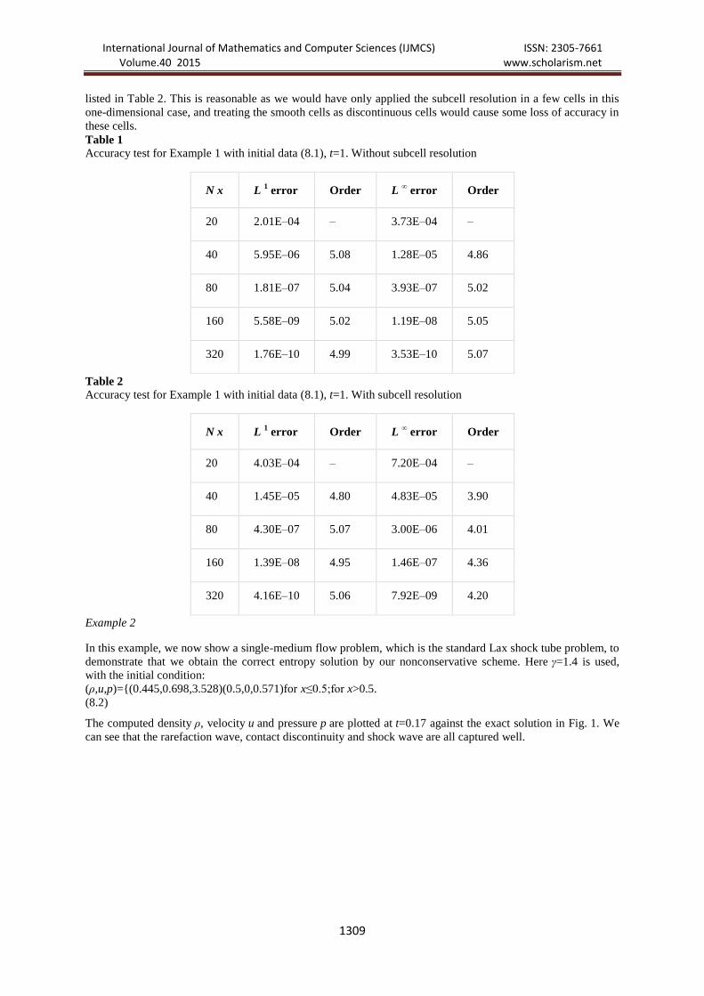
listed in Table 2. This is reasonable as we would have only applied the subcell resolution in a few cells in this

one-dimensional case, and treating the smooth cells as discontinuous cells would cause some loss of accuracy in

these cells.

Table 1 Accuracy test for Example 1 with initial data (8.1), t=1. Without subcell resolution

N x L 1 error Order L

∞ error Order

20 2.01E–04 – 3.73E–04 –

40 5.95E–06 5.08 1.28E–05 4.86

80 1.81E–07 5.04 3.93E–07 5.02

160 5.58E–09 5.02 1.19E–08 5.05

320 1.76E–10 4.99 3.53E–10 5.07

Table 2 Accuracy test for Example 1 with initial data (8.1), t=1. With subcell resolution

N x L 1 error Order L

∞ error Order

20 4.03E–04 – 7.20E–04 –

40 1.45E–05 4.80 4.83E–05 3.90

80 4.30E–07 5.07 3.00E–06 4.01

160 1.39E–08 4.95 1.46E–07 4.36

320 4.16E–10 5.06 7.92E–09 4.20

Example 2

In this example, we now show a single-medium flow problem, which is the standard Lax shock tube problem, to

demonstrate that we obtain the correct entropy solution by our nonconservative scheme. Here γ=1.4 is used,

with the initial condition:

(ρ,u,p)={(0.445,0.698,3.528)(0.5,0,0.571)for x≤0.5;for x>0.5.

(8.2)

The computed density ρ, velocity u and pressure p are plotted at t=0.17 against the exact solution in Fig. 1. We

can see that the rarefaction wave, contact discontinuity and shock wave are all captured well.

http://link.springer.com/article/10.1007/s10915-012-9578-7/fulltext.html#Tab2





1310

Fig. 1 Density, velocity and pressure for Example 2. t=0.17. Solid line: the exact solution. Symbol: the numerical

solution

Example 3

This example is a right moving shock for a single-medium flow. Here γ=5/3 is used, with the initial condition:

(ρ,u,p)=⎧⎩⎨(4114,9341−−−√,10)(1,0,1)for x≤0.5;for x>0.5.

(8.3)

We compute this problem on a domain [0,1]. A similar example (in Lagrangian form) is used in [3] to

demonstrate potential problems of nonconservative path-based Roe-type and Lax-Friedrichs (LxF)-type



1311

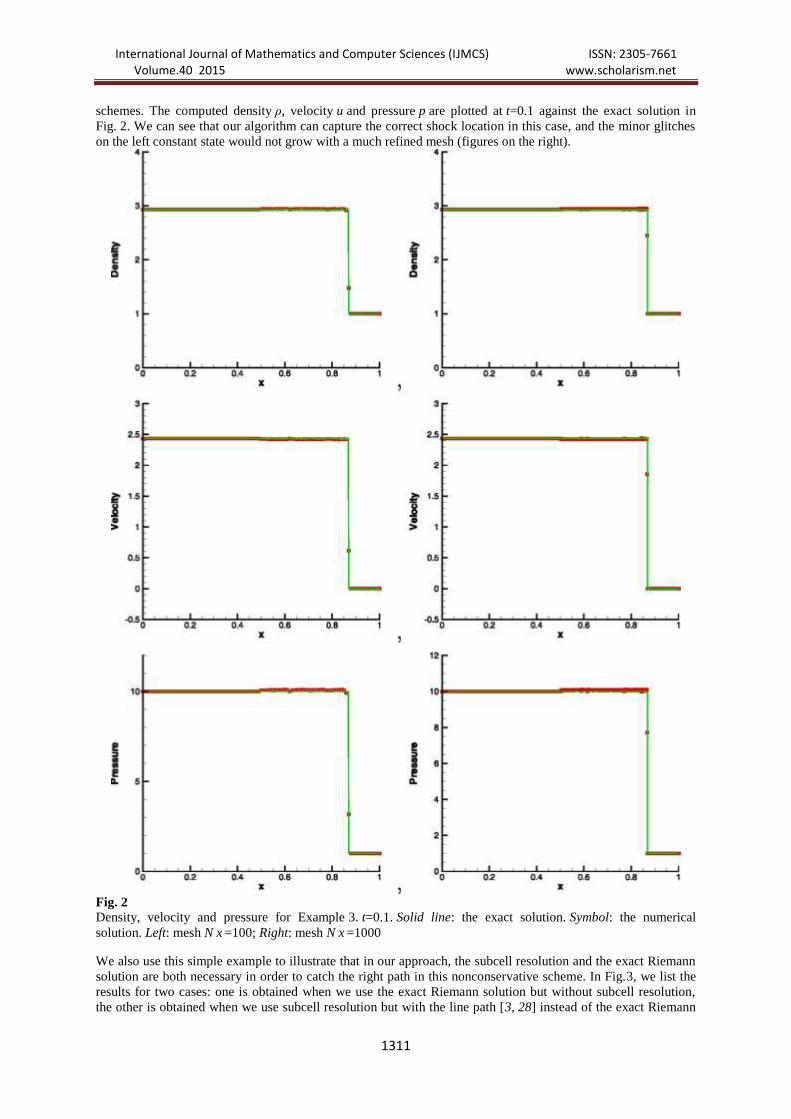
schemes. The computed density ρ, velocity u and pressure p are plotted at t=0.1 against the exact solution in

Fig. 2. We can see that our algorithm can capture the correct shock location in this case, and the minor glitches

on the left constant state would not grow with a much refined mesh (figures on the right).


solution. Left: mesh N x =100; Right: mesh N x =1000

We also use this simple example to illustrate that in our approach, the subcell resolution and the exact Riemann

solution are both necessary in order to catch the right path in this nonconservative scheme. In Fig.3, we list the

results for two cases: one is obtained when we use the exact Riemann solution but without subcell resolution,

the other is obtained when we use subcell resolution but with the line path [3, 28] instead of the exact Riemann






1312

solution, on a very refined mesh N x =1000. We can see that neither of them can catch the correct shock

solution.

Fig. 3 Density, velocity and pressure for Example 3. t=0.1. N x =1000. Solid line: the exact solution. Symbol: the

numerical solution. Left: exact Riemann solution without subcell resolution; Right: subcell resolution and with

the line path instead of the exact Riemann solution

Example 4

This is an air-helium shock tube problem taken from [14, 31, 36], with the initial condition:

(ρ,u,p,γ)={(1,0,1×105,1.4)(0.125,0,1×104,1.2)for x≤0.5;for x>0.5.





1313

(8.4)

The computed density ρ, velocity u and pressure p are plotted at t=0.0007 running with 495 time steps in our

code, against the exact solution in Fig. 4. We can see that the rarefaction wave, the contact discontinuity and the

shock wave are all captured well for this two-medium flow.


solution

Example 5



1314

This example is used to demonstrate the advantage of high order methods as in [29] for two-medium flows. It

contains both shocks and fine structures in smooth regions, which is a simple model for shock-turbulence

interactions. The initial discontinuity is right on the material interface and located at x=−4, the left and right

states for the initial discontinuity are

(ρ,u,p,γ)={(3.857143,2.629369,10.333333,1.4)(1+0.2sin(5x),0,1,5/3)for x<−4,for x>−4.

(8.5)

We compute the example up to time t=1.8 on a domain [−5, 5]. For comparison, we also show the results

obtained with a second order method, by replacing the fifth order WENO reconstruction with subcell resolution

in Sect. 4 with a second order ENO reconstruction [17, 42], and replacing the four-point Gauss-Lobatto

quadrature rule for the smooth integral term in Sect. 5.1 with a trapezoid rule. We plot the densities obtained by

the second order and the fifth order methods with N x =200 in Fig. 5. The solid line is the solution obtained by

the fifth order method with N x =1000 points, which can be considered as a converged reference solution. We

can find that the two methods can both capture the correct solution. However the result of the fifth order method

is in better agreement with the converged reference solution than the second order method, especially in the

region with fine structures, on this relatively coarse mesh. This is similar to the results in [50].

Fig. 5 Density, velocity and pressure for Example 5. t=1. Solid line: the converged reference solution for the fifth order

method with N x =1000. Symbol: the numerical solution with N x =200. Left: second order method;Right: fifth

order method

Example 6

This is a problem of a shock wave refracting at an air-helium interface with a reflected weak rarefaction wave

taken from [14, 31, 36], with the initial condition:

(ρ,u,p,γ)=⎧⎩⎨⎪⎪ (1.3333,0.3535105−−−√,1.5×105,1.4)(1,0,1×105,1.4)(0.1379,0,1×105,5/3)for x≤0.05,for 0.0

5<x≤0.5,for x>0.5.

(8.6)

The computed density ρ, velocity u and pressure p are plotted at t=0.0012 against the exact solution in Fig. 6.

The strength of the shock for this example is p L /p R =1.5, the computed results compare well with the exact

solutions, without oscillation around the material interface for the density.

Density, velocity and pressure for Example 6. t=0.0012. Solid line: the exact solution. Symbol: the numerical

solution

Concluding Remarks

In this paper, we have investigated using the WENO reconstruction with a subcell resolution technique when

applied to high order Roe-type schemes for nonconservative Euler equations. The subcell resolution is to

sharpen discontinuities, in order to remove or significantly reduce transitional points at discontinuities. The

technique has been shown to significantly improve the capturing of the correct discontinuity waves by defining

the correct path in the path integral at discontinuities. The smearing of discontinuities by shock capturing

schemes has transitional points at the discontinuities which do not necessarily land on the desired paths. We

have identified this numerical smearing as the most probable reason for the failure of schemes to converge to the

correct weak solution on the desired paths. The proposed subcell resolution technique within a Runge-Kutta













1315

time discretization seems to have robustness problems for very strong discontinuities, especially during

interactions of such discontinuities. An improvement on the robustness of the algorithms when transitional

points are removed or significantly reduced constitutes our future work.

Our discussion is restricted to the one-dimensional case. A preliminary study on the extension of our

methodology to two-dimensional problems (not reported in this paper), implemented in a dimension by

dimension fashion (not dimension splitting), has indicated limitations for some of the complex discontinuity

wave patterns. This may be due to the complication of two-dimensional waves and the limitation of the subcell

resolution technique to capture accurately the correct states and the corresponding paths at the discontinuities.

Further investigation of effective multi-dimensional algorithm in this context, for example, discontinuous

Galerkin (DG) method [11] and spectral finite volume method [32], also constitutes our future work.

Acknowledgements

We would like to thank Dr. Wei Liu for helpful discussions.

References

1.Abgrall, R.: How to prevent pressure oscillations in multicomponent flow calculations: a quasi-conservative

approach. J. Comput. Phys. 125, 150–160 (1996)MathSciNetMATHCrossRef

2.Abgrall, R., Karni, S.: Computations of compressible multifluids. J. Comput. Phys. 169, 594–623

(2001)MathSciNetMATHCrossRef

3.Abgrall, R., Karni, S.: A comment on the computation of non-conservative products. J. Comput. Phys. 229,

2759–2763 (2010)MathSciNetMATHCrossRef

4.Adalsteinsson, D., Sethian, J.A.: A fast level set method for propagating interfaces. J. Comput. Phys. 118,


5.van Brummelen, E.H., Koren, B.: A pressure-invariant conservative Godunov-type method for barotropic two-

fluid flows. J. Comput. Phys. 185, 289–308 (2003)MathSciNetMATHCrossRef

6.Castro, M.J., Fernández-Nieto, E.D., Ferreiro, A.M., García-Rodríguez, J.A., Parés, C.: High order extensions

of Roe schemes for two-dimensional nonconservative hyperbolic systems. J. Sci. Comput. 39, 67–114


7.Castro, M.J., Gallardo, J.M., Parés, C.: High order finite volume schemes based on reconstruction of states for

solving hyperbolic systems with nonconservative products. Application to shallow-water systems. Math.

Comput. 75, 1103–1134 (2006)MATHCrossRef

8.Castro, M.J., LeFloch, P., Muñoz-Ruiz, M.L., Parés, C.: Why many theories of shock waves are necessary:

Convergence error in formally path-consistent schemes. J. Comput. Phys. 227, 8107–8129


9.Chen, T.-J., Cooke, C.H.: On the Riemann problem for liquid or gas-liquid media. Int. J. Numer. Methods

Fluids 18, 529–541 (1994)MathSciNetMATHCrossRef

10.Cocchi, J.-P., Saurel, R.: A Riemann problem based method for the resolution of compressible multimaterial

flows. J. Comput. Phys. 137, 265–298 (1997)MathSciNetMATHCrossRef



http://www.ams.org/mathscinet-getitem?mr=1381808


http://dx.doi.org/10.1006/jcph.1996.0085






http://dx.doi.org/10.1016/j.jcp.2009.12.015






http://dx.doi.org/10.1016/S0021-9991(02)00058-X



http://dx.doi.org/10.1007/s10915-008-9250-4

http://www.emis.de/MATH-item?$1096.65082







http://dx.doi.org/10.1002/fld.1650180507





1316

11.Cockburn, B., Shu, C.-W.: The Runge-Kutta discontinuous Galerkin method for conservation laws V:

multidimensional systems. J. Comput. Phys. 141, 199–224 (1998)MathSciNetMATHCrossRef

12.Dal Maso, G., LeFloch, P., Murat, F.: Definition and weak stability of non-conservative products. J. Math.

Pure Appl. 74, 283–528 (1995)MathSciNetMATH

13.Dumbser, M., Toro, E.F.: A simple extension of the Osher Riemann solver to non-conservative hyperbolic

systems. J. Sci. Comput. 28, 70–88 (2011)MathSciNetMATHCrossRef

14.Fedkiw, R.P., Aslam, T., Merriman, B., Osher, S.: A non-oscillatory Eulerian approach to interfaces in

multimaterial flows (the Ghost Fluid Method). J. Comput. Phys. 152, 457–492


15.Fedkiw, R.P., Marquina, A., Merriman, B.: An isobaric fix for the overheating problem in multimaterial

compressible flows. J. Comput. Phys.128, 545–578 (1999)MathSciNetMATHCrossRef

16.Gottlieb, S., Ketcheson, D.I., Shu, C.-W.: High order strong stability preserving time discretizations. J. Sci.

Comput. 38, 251–289 (2009)MathSciNetMATHCrossRef

17.Harten, A.: ENO schemes with subcell resolution. J. Comput. Phys. 83, 128–184


18.Harten, A., Engquist, B., Osher, S., Chakravarthy, S.: Uniformly high order essentially non-oscillatory

schemes, III. J. Comput. Phys. 71, 231–303 (1987)MathSciNetMATHCrossRef

19.Harten, A., Hyman, J.M.: Self adjusting grid methods for one-dimensional hyperbolic conservation laws. J.

Comput. Phys. 50, 235–269 (1983)MathSciNetMATHCrossRef

20.Hou, T.Y., LeFloch, P.: Why nonconservative schemes converge to wrong solutions: error analysis. Math.

Comput. 62, 497–530 (1994)MathSciNetMATHCrossRef

21.Jiang, G., Peng, D.-P.: Weighted ENO schemes for Hamilton-Jacobi equations. SIAM J. Sci. Comput. 21,


22.Jiang, G., Shu, C.-W.: Efficient implementation of weighted ENO schemes. J. Comput. Phys. 126, 202–228


23.Karni, S.: Viscous shock profiles and primitive formulations. SIAM J. Numer. Anal. 29, 1592–1609


24.Karni, S.: Multicomponent flow calculations by a consistent primitive algorithm. J. Comput. Phys. 112, 31–

43 (1994)MathSciNetMATHCrossRef

25.Larrouturou, B.: How to preserve the mass fractions positivity when computing compressible multi-

component flow. J. Comput. Phys. 95, 31–43 (1991)MathSciNetCrossRef

26.LeVeque, R.J.: Finite Volume Methods for Hyperbolic Problems. Cambridge University Press, Cambridge

(2004)

27.Liu, T.G., Khoo, B.C., Wang, C.W.: The ghost fluid method for compressible gas-water simulation.

J. Comput. Phys. 204, 193–221 (2005)MathSciNetMATHCrossRef








http://dx.doi.org/10.1007/s10915-010-9400-3









http://dx.doi.org/10.1007/s10915-008-9239-z



http://dx.doi.org/10.1016/0021-9991(89)90226-X



http://dx.doi.org/10.1016/0021-9991(87)90031-3



http://dx.doi.org/10.1016/0021-9991(83)90066-9



http://dx.doi.org/10.1090/S0025-5718-1994-1201068-0



http://dx.doi.org/10.1137/S106482759732455X






http://dx.doi.org/10.1137/0729092










1317

28.Liu, T.G., Khoo, B.C., Yeo, K.S.: The simulation of compressible multi-medium flow. Part I: a new

methodology with applications to 1D gas-gas and gas-water cases. Comput. Fluids 30, 291–314

(2001)MATHCrossRef

29.Liu, T.G., Khoo, B.C., Yeo, K.S.: The simulation of compressible multi-medium flow. Part II: applications to

2D underwater shock refraction. Comput. Fluids 30, 315–337 (2001)CrossRef

30.Liu, T.G., Khoo, B.C., Yeo, K.S.: Ghost fluid method for strong shock impacting on material interface. J.

Comput. Phys. 190, 651–681 (2003)MATHCrossRef

31.Liu, W., Yuan, Y., Shu, C.-W.: A conservative modification to the ghost fluid method for compressible

multiphase flows. Commun. Comput. Phys. 10, 1238–1228 (2011)MathSciNet

32.Liu, X.-D., Osher, S., Chan, T.: Weighted essentially non-oscillatory schemes. J. Comput. Phys. 115, 200–

212 (1994)MathSciNetMATHCrossRef

33.Mulder, W., Osher, S., Sethian, J.A.: Computing interface motion in compressible gas dynamics. J. Comput.

Phys. 100, 209–228 (1992)MathSciNetMATHCrossRef

34.Osher, S., Fedkiw, R.P.: Level Set Methods and Dynamic Implicit Surfaces. Springer, Berlin (2003)MATH

35.Parés, C.: Numerical methods for nonconservative hyperbolic systems: a theoretical framework. SIAM J.

Numer. Anal. 44, 300–321 (2006)MathSciNetMATHCrossRef

36.Qiu, J., Liu, T., Khoo, B.C.: Runge-Kutta discontinuous Galerkin methods for compressible two-medium

flow simulations: one-dimensional case. J. Comput. Phys. 222, 353–373 (2007)MathSciNetMATHCrossRef

37.Qiu, J., Liu, T., Khoo, B.C.: Simulations of compressible two-medium flow by Runge-Kutta discontinuous

Galerkin methods with the Ghost Fluid Method. Commun. Comput. Phys. 3, 479–504 (2008)MathSciNetMATH

38.Quirk, J.J., Karni, S.: On the dynamics of a shock-bubble interaction. J. Fluid Mech. 318, 129–163

(1996)MATHCrossRef

39.Shi, J., Hu, C., Shu, C.-W.: A technique of treating negative weights in WENO schemes. J. Comput.

Phys. 175, 108–127 (2002)MATHCrossRef

40.Shu, C.-W.: Essentially non-oscillatory and weighted essentially non-oscillatory schemes for hyperbolic

conservation laws. In: Cockburn, B., Johnson, C., Shu, C.-W., Tadmor, E. (eds.) Advanced Numerical

Approximation of Nonlinear Hyperbolic Equations. Lecture Notes in Mathematics, vol. 1697, pp. 325–432.

Springer, Berlin (1998) (Editor: A. Quarteroni)CrossRef

41.Shu, C.-W., Osher, S.: Efficient implementation of essentially non-oscillatory shock-capturing schemes. J.


42.Shu, C.-W., Osher, S.: Efficient implementation of essentially non-oscillatory shock-capturing schemes II. J.




http://dx.doi.org/10.1016/S0045-7930(00)00021-9









http://dx.doi.org/10.1016/0021-9991(92)90229-R




http://dx.doi.org/10.1137/050628052










http://dx.doi.org/10.1007/BFb0096355



http://dx.doi.org/10.1016/0021-9991(88)90177-5



http://dx.doi.org/10.1016/0021-9991(89)90222-2

weno scheme with subcell resolution for computing ...scholarism.net/fulltext/ijmcs20154004.pdf ·...

Documents