high-order weno schemes for hamilton–jacobi equations …yzhang10/triweno.pdf · high-order weno...

HIGH-ORDER WENO SCHEMES FOR HAMILTON–JACOBIEQUATIONS ON TRIANGULAR MESHES∗

YONG-TAO ZHANG† AND CHI-WANG SHU†

SIAM J. SCI. COMPUT. c© 2003 Society for Industrial and Applied MathematicsVol. 24, No. 3, pp. 1005–1030

Abstract. In this paper we construct high-order weighted essentially nonoscillatory (WENO)schemes for solving the nonlinear Hamilton–Jacobi equations on two-dimensional unstructuredmeshes. The main ideas are nodal based approximations, the usage of monotone Hamiltoniansas building blocks on unstructured meshes, nonlinear weights using smooth indicators of second andhigher derivatives, and a strategy to choose diversified smaller stencils to make up the bigger stencilin the WENO procedure. Both third-order and fourth-order WENO schemes using combinations ofsecond-order approximations with nonlinear weights are constructed. Extensive numerical experi-ments are performed to demonstrate the stability and accuracy of the methods. High-order accuracyin smooth regions, good resolution of derivative singularities, and convergence to viscosity solutionsare observed.

Key words. weighted essentially nonoscillatory schemes, Hamilton–Jacobi equations, high-orderaccuracy, unstructured mesh

AMS subject classification. 65M99

PII. S1064827501396798

1. Introduction. In this paper, we consider the numerical solution of Hamilton–Jacobi (H-J) equations

φt + H(φx1 , . . ., φxd) = 0, φ(x, 0) = φ0(x).(1.1)

Such equations appear often in applications, such as in optimal control, differentialgames, image processing and computer vision, and geometric optics. With the pop-ularity of level set methods [14] the necessity to have good algorithms to solve H-Jequations becomes even more obvious.

There have been many papers in the literature developing numerical methodsto solve H-J equations. In a certain sense H-J equations are easier to solve thantheir conservation laws counterparts because the solutions here are smoother: typicalsolutions are continuous with possibly discontinuous derivatives.

For a structured mesh, finite difference methods similar to those developed forconservation laws could be easily designed. Thus we have the earlier second-orderENO schemes of Osher and Sethian [14], higher-order ENO schemes of Osher andShu [15], higher-order weighted ENO (WENO) schemes of Jiang and Peng [9], andcentral high resolution schemes of Lin and Tadmor [12], among many others.

However, for unstructured meshes there are conceptional difficulties in designingschemes such as finite volume schemes and finite element schemes, which are veryuseful for conservation laws. The problem arises because the H-J equations cannotbe written in a “conservation form,” suitable for integration by parts, which is thebackbone of finite volume and finite element methods. Thus algorithms, especially

∗Received by the editors October 22, 2001; accepted for publication (in revised form) June24, 2002; published electronically January 23, 2003. This research was supported by ARO grantDAAD19-00-1-0405, NSF grants DMS-9804985 and ECS-9906606, NASA Langley grant NCC1-01035and contract NAS1-97046, while the second author was in residence at ICASE, NASA Langley Re-search Center, Hampton, VA 23681-2199, and AFOSR grant F49620-99-1-0077.

http://www.siam.org/journals/sisc/24-3/39679.html†Division of Applied Mathematics, Brown University, Providence, RI 02912 ([email protected],

[email protected]).

1005

1006 YONG-TAO ZHANG AND CHI-WANG SHU

high-order algorithms for H-J equations on unstructured meshes, are relatively few.We have the very good first- and second-order finite volume–type schemes of Abgrall[2] and ENO- or limiter-type high-order version of Augoula and Abgrall [4]. Themonotone Hamiltonians developed in [2] are used in this paper as building blocks.We also have the continuous finite element methods of Barth and Sethian [6] and thediscontinuous Galerkin methods of Hu and Shu [7]. However, the formulation of thefinite element methods in [7] actually uses the differentiated version of H-J, which is asystem of conservation laws. It would be desirable in many situations to use directlyH-J on an unstructured mesh and still obtain high-order, nonoscillatory numericalresults. The algorithms developed in this paper fulfills this purpose.

The WENO methodology adopted in this paper can be traced back to the earlierwork for conservation laws started in [13] for a third-order finite volume version in onespace dimension and in [10] for third- and fifth-order finite difference WENO schemesin multispace dimensions with a general framework for the design of the smoothnessindicators and nonlinear weights. The techniques most relevant to the current paperare the third- and fourth-order finite volume WENO schemes for two-dimensional(2D) conservation laws in general triangulations [8] and the finite difference WENOschemes for H-J equations [9]. However, significant new components of the algorithmshave been developed in this paper to deal with the additional difficulty caused by the“nonconservation” form of the H-J equations and unstructured meshes. These includenodal based approximations, the usage of monotone Hamiltonians as building blockson unstructured meshes, nonlinear weights using smooth indicators of second andhigher derivatives, and a strategy to choose diversified smaller stencils to make up thebigger stencil in the WENO procedure. Both third-order and fourth-order WENOschemes using combinations of second-order approximations with nonlinear weightsare constructed. Extensive numerical experiments are performed to demonstrate thestability and accuracy of the methods. High-order accuracy in smooth regions, goodresolution of derivative singularities, and convergence to viscosity solutions are ob-served.

The algorithm is developed in section 2. Section 3 contains numerical exam-ples verifying the stability, convergence, and accuracy of the algorithms. Concludingremarks are given in section 4.

2. The WENO algorithm for 2D unstructured mesh. In this section wedevelop third- and fourth-order WENO schemes on unstructured meshes in two di-mensions for the H-J equations.

2.1. The framework. We take d = 2 in (1.1), and use x, y instead of x1, x2:

φt + H(φx, φy) = 0, φ(x, y, 0) = φ0(x, y).(2.1)

The equation (2.1) is solved in the domain Ω, which has a triangulation Th consistingof triangles. The nodes will be named by their indices 0 ≤ i ≤ N , with a total of N+1nodes. For every node i, we define the ki+1 angular sectors T0, . . ., Tki meeting at thepoint i; they are the inner angles at node i of the triangles having i as a vertex. Theindexing of the angular sectors is ordered counterclockwise. nl+ 1

2is the unit vector

of the half-line Dl+ 12

= Tl

⋂Tl+1, and θl is the inner angle of sector Tl, 0 ≤ l ≤ ki;

see Figure 2.1.We will denote by φi the numerical approximation to the viscosity solution of (2.1)

at node i. (∇φ)0, . . ., (∇φ)ki will, respectively, represent the numerical approximationof ∇φ at node i in each angular sector T0, . . ., Tki .

WENO SCHEMES FOR HJ EQUATIONS ON TRIANGULAR MESHES 1007

i

Tl+1

Tl

Tl−1

nl+1/2

θl

Fig. 2.1. Node i and its angular sectors.

An important building block for the algorithms in this paper is the Lax–Friedrichs-type monotone Hamiltonian for arbitrary triangulations developed by Abgrall in [2],which is a generalization of the Lax–Friedrichs monotone Hamiltonian for Cartesianmeshes in Osher and Shu [15]. This monotone Hamiltonian is given by

H((∇φ)0, . . ., (∇φ)ki) = H

ki∑l=0

θl(∇φ)l

2π

− α

π

ki∑l=0

βl+ 12

((∇φ)l + (∇φ)l+1

2

)· nl+ 1

2,

(2.2)

where

βl+ 12

= tan

(θl2

)+ tan

(θl+1

2

), α = max

max

A≤u≤BC≤v≤D

|H1(u, v)|, maxA≤u≤BC≤v≤D

|H2(u, v)|.

Here H1 and H2 are the partial derivatives of H with respect to φx and φy, re-spectively, or the Lipschitz constants of H with respect to φx and φy, if H is notdifferentiable. [A,B] is the value range for (φx)l, and [C,D] is the value range for(φy)l, over 0 ≤ l ≤ ki for the local Lax–Friedrichs Hamiltonian, and over 0 ≤ l ≤ kiand 0 ≤ i ≤ N for the global Lax–Friedrichs Hamiltonian.

The H in (2.2) defines a monotone Hamiltonian. It is Lipschitz continuous in allarguments and is consistent with H, i.e., H(∇φ, . . .,∇φ) = H(∇φ). Hence if we havehigh-order approximations to ∇φ at node i in every angular sector, the numericalHamiltonian H will be a high-order approximation to H.

The semidiscrete scheme is thus given by

d

dtφi(t) + H((∇φ)0, . . ., (∇φ)ki) = 0(2.3)


and it is discretized in time by the high order nonlinearly stable Runge–Kutta timediscretization in [18]. If the spatial dimension reduces to one, the numerical Hamil-tonian (2.2) will reduce to the local or global Lax–Friedrichs Hamiltonian [15]:

H(u−, u+) = H

(u− + u+

2

)− 1

2α(u+ − u−)(2.4)

with α = maxA≤u≤B |H ′(u)|. If the maximum for computing α is taken over therange covered by u− and u+, we get the local Lax–Friedrichs Hamiltonian; if it is alsotaken over all grid points, we get the global Lax–Friedrichs Hamiltonian.

2.2. Linear schemes. Now we discuss how to construct a high-order approx-imation for ∇φ in every angular sector of every node. Let P k denote the set of 2Dpolynomials of degree less than or equal to k. We use Lagrange interpolations as fol-lows: given a smooth function φ, and a triangulation with triangles 0,1, . . .,Mand nodes 0, 1, 2, . . ., N, we would like to construct, for each triangle i, a polyno-mial p(x, y) ∈ P k such that p(xl, yl) = φ(xl, yl), where (xl, yl) are the coordinates ofthe three nodes of the triangle i and a few neighboring nodes. p(x, y) would thusbe a (k + 1)st-order approximation to φ on the cell i.

Because kth degree polynomial p(x, y) has K = (k+1)(k+2)2 degrees of freedom, we

need to use the information of at least K nodes. In addition to the three nodes of thetriangle i, we may take the other K − 3 nodes from the neighboring cells aroundtriangle i. We rename these K nodes as Si = M1,M2, . . .,MK; Si is called a bigstencil for the triangle i. Let (xi, yi) be the barycenter of i. Define ξ = (x−xi)/hi,η = (y − yi)/hi, where hi =

√|i| with |i| denoting the area of the triangle i;then we can write p(x, y) as

p(x, y) =

k∑j=0

∑s+r=j

asrξsηr.

Using the K interpolation conditions,

p(Ml) = φ(Ml), l = 1, 2, . . .,K,

we get a K × K linear system for the K unknowns asr. The normalized variablesξ, η are used to make the condition number of the linear system independent of meshsizes.

It is well known that in two and higher dimensions such interpolation problemsis not always well defined. The linear system can be very ill-conditioned or evensingular; in such cases we would have to add more nodes to the big stencil Si from theneighboring cells around triangle i to obtain an overdetermined linear system andthen use the least-squares method to solve it. We remark that this ill-conditioningcomes from both the geometric distribution of the nodes, for which we could donothing other than changing the mesh, and from the choice of basis functions in theinterpolation. For higher-order methods, a closer to orthogonal basis rather thanξsηr would be preferred, such as the procedure using barycentric coordinates in [1]and [3]. However, for the third- and fourth-order cases considered in this paper, wehave chosen to use ξsηr for simplicity.

After we have obtained the approximation polynomial p(x, y) on the triangle i,∇p will be a kth-order approximation for ∇φ on i. Hence we get the high-orderapproximation ∇p(xl, yl) to ∇φ(xl, yl), for any one of the three vertices (xl, yl) of thetriangle i, in the relevant angular sectors.


i j

k1

G

4

2

5

9

3

6

7

8

Fig. 2.2. The nodes used for the big stencil of the third-order scheme.

2.2.1. Third-order linear schemes. A scheme is called linear if it is linearwhen applied to a linear equation with constant coefficients. We need a third-orderapproximation for ∇φ to construct a third-order linear scheme, hence we need a cubicpolynomial interpolation. A cubic polynomial p3 has 10 degrees of freedom. We willuse some or all of the nodes shown in Figure 2.2 to form our big stencil. For extremelydistorted meshes the number of nodes in Figure 2.2 may be fewer than the required 10.In such extreme cases we would need to expand the choice for the big stencil, followingthe idea in Figure 2.3 in the next subsection for the fourth-order scheme. For ourtarget triangle 0, which has three vertices i, j, k and the barycenter G, we need toconstruct a cubic polynomial p3; then ∇p3 will be a third-order approximation for ∇φon 0, and the values of ∇p3 at points i, j, and k will be third-order approximationsfor ∇φ at the angular sector 0 of nodes i, j, and k. We name the nodes of theneighboring triangles of triangle 0 as follows: nodes 1, 2, 3 are the nodes (otherthan i, j, k) of neighbors of 0, nodes 4, 5, 6, 7, 8, 9 (other than 1, 2, 3, i, j, k) arethe nodes of the neighbors of the three neighboring triangles of 0. Notice that thepoints 4, 5, 6, 7, 8, 9 do not have to be six distinct points. For example, the points 5and 9 could be the same point.

Our interpolation points are nodes taken from a sorted node set. An orderingis given in the set so that, when the nodes are chosen sequentially from it to formthe big stencil S0, the target triangle 0 remains central to avoid serious downwindbias which could lead to linear instability. Referring to Figure 2.2, our interpolationpoints for the polynomial p3 include nodes i, j, k and the nodes taken from the sortedset: W = 1, 2, 3, 4, 5, 6, 7, 8, 9. The detailed procedure to determine the big stencilS0 for the target triangle 0 is given below.

Procedure 2.1. The choice of the big stencil for the third-order scheme.

1. Referring to Figure 2.2, form a sorted node set: W = 1, 2, 3, 4, 5, 6, 7, 8, 9.In extreme cases when this set does not contain enough distinct points, wemay need to add more points from the next layer of neighbors.


2. To start with, we take S0 = i, j, k, 1, 2, 3, 4, 5, 6, 7. Use this stencil S0 toform the 10 × 10 interpolation coefficient matrix A.

3. Compute the reciprocal condition number c of A. This is provided by mostlinear solvers. If c ≥ δ for some threshold δ, we have obtained the final stencilS0. Otherwise, add the next node in W (i.e., node 8) to S0. Use the 11 nodesin S0 as interpolation points to get the 11 × 10 least square interpolation co-efficient matrix A. Judge the reciprocal condition number c again. Continuedoing this until c ≥ δ is satisfied. In our computation, we have taken δ = 10−3

as a good threshold after extensive numerical experiments. Notice that, sincewe have normalized the coordinates, this threshold does not change when themesh is scaled uniformly in all directions. For all the triangulations we havetested, at most 12 nodes are needed in S0 to reach the condition c ≥ δ.

Remark 2.1. The ordering in the sorted node set W is important to make thetarget cell 0 sufficiently “central” in the stencil, thus avoiding S0 to be seriouslydownwind biased, which could lead to linear instability. Linear instability is indeedobserved in our numerical experiments when 1, 2, 3 are not forced to be in S0.

We now have obtained the big stencil S0 and its associated cubic polynomial p3.For each node (xl, yl) in 0, ∇p3(xl, yl) is a third-order approximation to ∇φ(xl, yl).In order to construct a high-order WENO scheme, an important step is to obtain ahigh-order approximation using a linear combination of lower-order approximations.We will use a linear combination of second-order approximations to get the samethird-order approximation to ∇φ(xl, yl) as ∇p3(xl, yl), i.e., we require

∂

∂xp3(xl, yl) =

q∑s=1

γs,x∂

∂xps(xl, yl),

∂

∂yp3(xl, yl) =

q∑s=1

γs,y∂

∂yps(xl, yl),(2.5)

where ps are quadratic interpolation polynomials, and γs,x and γs,y are the linearweights for the x-directional derivative and the y-directional derivative, respectively,for s = 1, . . ., q. The linear weights are constants depending only on the local geometryof the mesh. The equalities in (2.5) should hold for any choices of the function φ.

Notice that to get a second-order approximation for the derivatives ∇φ(xl, yl),we need a quadratic interpolation polynomial. According to the argument in [8],the cubic polynomial p3(x, y) has four more degrees of freedom than each quadraticpolynomial ps(x, y), namely x3, x2y, xy2, y3. For the six degrees of freedom 1, x,y, x2, xy, y2, if we take φ = 1, φ = x, φ = y, φ = x2, φ = xy, and φ = y2, theequalities in (2.5) will hold for all these cases under only one constraint each on γs,xand γs,y, namely

∑qs=1 γs,x = 1 and

∑qs=1 γs,y = 1, because p3 and ps all reproduce

these functions exactly. Hence we should only need q ≥ 5. We take q = 5 in ourscheme.

We now need q = 5 small stencils Γs, s = 1, . . ., 5 for the target triangle 0,satisfying S0 =

⋃5s=1 Γs, and every quadratic polynomial ps is associated with a

small stencil Γs. In our third-order scheme, the small stencils will be the same forboth directions x, y and all three nodes i, j, k in 0. However, the linear weightsγs,x, γs,y can be different for different nodes i, j, k and different directions x, y. Becauseeach quadratic polynomial has six degrees of freedom, the number of nodes in Γs

must be at least six. To build a small stencil Γs, we start from several candidates

Γ(r)s , r = 1, 2, . . ., ns. These candidates are constructed by first taking a point A

(r)s as

the “center,” then finding at least six nodes from S0 which have the shortest distances

from A(r)s and can generate the interpolation coefficient matrix with a good condition

number, using the method of Procedure 2.1. We then choose the best Γs among Γ(r)s ,


r = 1, . . ., ns for every s = 1, . . ., 5. Here “best” means that by using this group ofsmall stencils, the linear weights γs,x, γs,y, s = 1, . . ., 5 for all three nodes i, j, k, areeither all positive or have the smallest possible negative values in magnitude. Thedetails of the algorithm is described in the following procedure.

Procedure 2.2. The third-order linear scheme. For every triangle l, l = 1, . . ., N ,do steps 1–5:

1. Follow Procedure 2.1 to obtain the big stencil Sl for l.

2. For s = 1, . . ., 5, find the set Ws = Γ(r)s , r = 1, 2, . . ., ns, which are the

candidate small stencils for the sth small stencil. We use the following method

to find the Γ(r)s in Ws: First, nodes i, j, k are always included in every Γ

(r)s ;

then, we take a point A(r)s as the center of Γ

(r)s , detailed below, and find at

least 3 additional nodes other than i, j, k from Sl which satisfy the following

two conditions: (1) they have the shortest distances from A(r)s ; and (2) taking

them and the nodes i, j, k as the interpolation points, we will obtain theinterpolation coefficient matrix A with a good condition number, namely thereciprocal condition number c of A satisfies c ≥ δ with the same thresholdδ = 10−3. For the triangulations we have tested, at most 8 nodes are used to

reach this threshold value. Finally, the center of the candidate stencils A(r)s ,

r = 1, . . ., ns; s = 1, . . ., 5 are taken from the nodes around l (see Figure 2.2)as follows:

• A(1)1 = point G, n1 = 1;

• A(1)2 = node 1, A

(2)2 = node 4, A

(3)2 = node 7, n2 = 3;

• A(1)3 = node 2, A

(2)3 = node 5, A

(3)3 = node 8, n3 = 3;

• A(1)4 = node 3, A

(2)4 = node 6, A

(3)4 = node 9, n4 = 3;

• A(r)5 9

r=1 = nodes 4, 5, 6, 7, 8, 9 and the middle points of nodes 4 and 8,5 and 9, 6 and 7. n5 ≤ 9.

3. By taking one small stencil Γ(rs)s from each Ws, s = 1, . . ., 5, to form a group,

we obtain n1×n2×· · ·×n5 groups of small stencils. We eliminate the groupswhich contain the same small stencils and also eliminate the groups which donot satisfy the condition

5⋃s=1

Γ(rs)s = Sl.

According to every group Γ(rs)s , s = 1, . . ., 5 of small stencils, we have 5

quadratic polynomials p(rs)s 5

s=1. We evaluate ∂∂xp

(rs)s and ∂

∂yp(rs)s at points

i, j, k, to obtain second-order approximation values for ∇φ at the three ver-tices of the triangle l. We remark that for practical implementation, we donot use the polynomial itself, but compute a series of constants alml=1 whichdepend on the local geometry only, such that

∂

∂xp(rs)s (xn, yn) =

m∑l=1

alφl,(2.6)

where every constant al corresponds to one node in the stencil Γ(rs)s and m

is the total number of nodes in Γ(rs)s . For every vertex (xn, yn) of triangle

l, we obtain a series of such constants. And for the y-directional partialderivative, we compute the corresponding constants too.


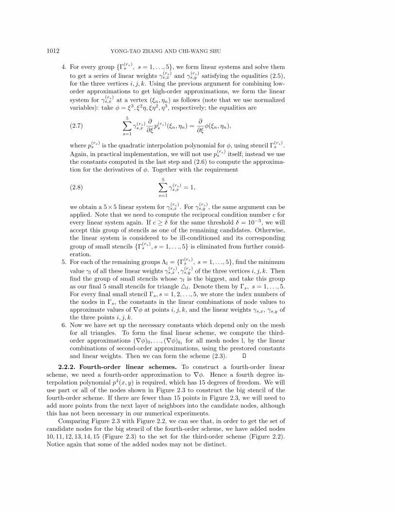
4. For every group Γ(rs)s , s = 1, . . ., 5, we form linear systems and solve them

to get a series of linear weights γ(rs)s,x and γ

(rs)s,y satisfying the equalities (2.5),

for the three vertices i, j, k. Using the previous argument for combining low-order approximations to get high-order approximations, we form the linear

system for γ(rs)s,x at a vertex (ξn, ηn) as follows (note that we use normalized

variables): take φ = ξ3, ξ2η, ξη2, η3, respectively; the equalities are

5∑s=1

γ(rs)s,x

∂

∂ξp(rs)s (ξn, ηn) =

∂

∂ξφ(ξn, ηn),(2.7)

where p(rs)s is the quadratic interpolation polynomial for φ, using stencil Γ

(rs)s .

Again, in practical implementation, we will not use p(rs)s itself; instead we use

the constants computed in the last step and (2.6) to compute the approxima-tion for the derivatives of φ. Together with the requirement

5∑s=1

γ(rs)s,x = 1,(2.8)

we obtain a 5×5 linear system for γ(rs)s,x . For γ

(rs)s,y , the same argument can be

applied. Note that we need to compute the reciprocal condition number c forevery linear system again. If c ≥ δ for the same threshold δ = 10−3, we willaccept this group of stencils as one of the remaining candidates. Otherwise,the linear system is considered to be ill-conditioned and its corresponding

group of small stencils Γ(rs)s , s = 1, . . ., 5 is eliminated from further consid-

eration.5. For each of the remaining groups Λl = Γ

(rs)s , s = 1, . . ., 5, find the minimum

value γl of all these linear weights γ(rs)s,x , γ

(rs)s,y of the three vertices i, j, k. Then

find the group of small stencils whose γl is the biggest, and take this groupas our final 5 small stencils for triangle l. Denote them by Γs, s = 1, . . ., 5.For every final small stencil Γs, s = 1, 2, . . ., 5, we store the index numbers ofthe nodes in Γs, the constants in the linear combinations of node values toapproximate values of ∇φ at points i, j, k, and the linear weights γs,x, γs,y ofthe three points i, j, k.

6. Now we have set up the necessary constants which depend only on the meshfor all triangles. To form the final linear scheme, we compute the third-order approximations (∇φ)0, . . ., (∇φ)kl

for all mesh nodes l, by the linearcombinations of second-order approximations, using the prestored constantsand linear weights. Then we can form the scheme (2.3).

2.2.2. Fourth-order linear schemes. To construct a fourth-order linearscheme, we need a fourth-order approximation to ∇φ. Hence a fourth degree in-terpolation polynomial p4(x, y) is required, which has 15 degrees of freedom. We willuse part or all of the nodes shown in Figure 2.3 to construct the big stencil of thefourth-order scheme. If there are fewer than 15 points in Figure 2.3, we will need toadd more points from the next layer of neighbors into the candidate nodes, althoughthis has not been necessary in our numerical experiments.

Comparing Figure 2.3 with Figure 2.2, we can see that, in order to get the set ofcandidate nodes for the big stencil of the fourth-order scheme, we have added nodes10, 11, 12, 13, 14, 15 (Figure 2.3) to the set for the third-order scheme (Figure 2.2).Notice again that some of the added nodes may not be distinct.


i j

k

1

5

G

10

13

11

14

1215

4

8

2

9

3

6

7

Fig. 2.3. The nodes used for the big stencil of the fourth-order scheme.

As in Procedure 2.1, in order to avoid possible linear instability due to seriousdownwinding, we first give an ordering to the candidate nodes. Referring to Figure 2.3,our interpolation points for the polynomial p4 include nodes i, j, k and the nodes takenfrom the sorted set: W = 1, 2, 3, 4, 5, 6, 7, 8, 9, 10, 11, 12, 13, 14, 15. The detailedprocedure to determine the big stencil S0 for the target triangle 0 is given below.

Procedure 2.3. The big stencil of the fourth-order scheme.

1. Referring to Figure 2.3, form a sorted node set: W = 1, 2, 3, 4, 5, 6, 7, 8, 9, 10,11, 12, 13, 14, 15. In extreme cases when this set does not contain enough dis-tinct points, we may need to add more points from the next layer of neighbors.

2. To start with, we take S0 = i, j, k, 1, 2, 3, 4, 5, 6, 7, 8, 9, 10, 11, 12. Use thisstencil S0 to form the 15 × 15 interpolation coefficient matrix A.

3. Compute the reciprocal condition number c of A. If c ≥ δ for the samethreshold δ = 10−3, we have obtained the final big stencil S0. Otherwise, weadd the next node (i.e., node 13) in W to S0. Then we obtain the 16 × 15interpolation coefficient matrix A associated with this S0, an overdeterminedsystem which can be solved by the least square procedure. Compute thereciprocal condition number of A and check whether c ≥ δ again. Repeatthis if necessary until c ≥ δ is satisfied. In our numerical tests, at most 16nodes are needed in S0 to reach our threshold value in all the cases.

We emphasize again that the ordering for the nodes as in Figure 2.3 is importantto guarantee the chosen stencil to yield to linear stability of the scheme.

Remark 2.2. Figures 2.2 and 2.3 are just the typical distribution of nodes arounda target triangle. If the node distribution is different from that in Figures 2.2 and 2.3because some nodes coincide, then the next level of neighboring nodes is added intothe candidate node set, and these extra nodes are also sorted to make the target cellcentral. We can always add more nodes into our candidate node set if the nodes arenot enough to reach our threshold value of condition number.

Using the big stencil, we obtain the fourth-order approximation ∇p4 for ∇φ.


The key step in building our fourth-order WENO scheme is to get a fourth-orderapproximation for ∇φ based on lower-order approximations. We still would like toconstruct several second-order approximations whose weighted average will give thesame result as ∇p4 at each angular sector of every node, i.e.,

∂

∂xp4(xl, yl) =

q∑s=1

γs,x∂

∂xps,x(xl, yl),

∂

∂yp4(xl, yl) =

q∑s=1

γs,y∂

∂yps,y(xl, yl),

(2.9)

where ps,x, ps,y are the quadratic interpolation polynomials and γs,x, γs,y are the linearweights.

Remark 2.3. The reason that we still use second-order approximations, not third-order ones, as the lower-order approximations is that each second-order approximationneeds fewer nodes in the big stencil; thus it is easier to make the small stencils to besufficiently diversified, which is important for the WENO technique to function wellnear discontinuous derivatives in the solutions. We have encountered difficulties inobtaining nonoscillatory results converging to the correct viscosity solutions for someof the more demanding test cases when third-order building blocks are used insteadof the second-order ones.

We now determine the value of q, which is the number of small stencils, in theequalities (2.9). Because p4 has nine more degrees of freedom than the quadratic poly-nomials ps,x, ps,y, i.e., x3, x2y, xy2, y3, x4, x3y, x2y2, xy3, y4, according to our previousargument, we would need q ≥ 10. We take q = 10 in our fourth-order scheme. Theprocedure to find all the small stencils is described below.

Procedure 2.4. The fourth-order linear scheme.For every triangle l, l = 1, . . ., N , do steps 1–3:1. Follow Procedure 2.3 to obtain the big stencil Sl for l.2. For each of the six approximations (φx, φy at vertices i, j, k of l), find 10

small stencils, respectively. Let Γs,x, s = 1, . . ., 10 denote the small stencilsto approximate φx at vertex i. To find them, we first determine 10 preliminarysmall stencils Γ0

s, s = 1, . . ., 10 as follows (see Figure 2.3):(1) Include nodes i, j, k, 1, 2, 3 in Γ0

1.(2) Include nodes i, j, k, 1, 4, 7 in Γ0



4.(5) Include nodes i, j, k in all Γ0

s, s = 5, 6, . . ., 10.(6) Take points As, s = 1, . . ., 10 as the center of Γ0

s10s=1, where A1 = point

G, A2 = node 1, A3 = node 2, A4 = node 3, A5 = node 10, A6 = node13, A7 = node 11, A8 = node 14, A9 = node 12, and A10 = node 15.

(7) Obtain 6 nodes for each of Γ0s10

s=1. There are already 6 points inΓ0

s4s=1. For Γ0

s10s=5, we add 3 nodes (other than i, j, k) from Sl to

each of them, which have the shortest distances from As. Then use Γ0s

to get the interpolation coefficient matrix, and judge the reciprocal con-dition number c of the matrix. If c reaches our threshold value δ = 10−3,then Γ0

s is found. Otherwise add one different node from Sl to Γ0s, which

has the shortest distance from As. Continue this until c ≥ δ is satisfied.(8) All of the 6 approximations (to φx, φy at vertices i, j, k of l) have the

common 10 preliminary small stencils Γ0s, s = 1, . . ., 10.

Now we come to determine Γs,x, s = 1, . . ., 10. Our goal is that the coeffi-

cient matrix A of the 10×10 linear system, which is obtained from Γs,x10s=1


and used to compute the linear weights, has a good condition number. Fors = 1, 2, . . ., 10, we perform the following steps:(1) Taking the original small stencil Γ0

s as the interpolation stencil, computethe constants alml=1, which depend on the mesh only and are the coef-ficients in the linear combination of function values at the nodes in Γ0

s

to get the second-order approximation to φx at vertex i.(2) Form the sth column of the matrix A. Let art be the elements of the

matrix A. Take the 9 functions φ(r)10r=2 = ξ3, ξ2η, ξη2, η3, ξ4, ξ3η, ξ2η2,

ξη3, η4, respectively, and let p(r)s,x be the second-order interpolation poly-

nomial for φ(r), r = 2, . . ., 10; then a1s = 1, and

ars =∂

∂ξp(r)s,x(ξi, ηi), r = 2, . . ., 10,(2.10)

where (ξi, ηi) is the coordinate of vertex i. (Again note that we usenormalized variables.) We use the constants computed at the last stepto implement this and will not need to use the polynomials themselves.

(3) Now A has s columns and is a 10 × s matrix. Compute its reciprocalcondition number c. If c ≥ δ, take the current small stencil as our sthsmall stencil Γs,x. Otherwise, change one node, which is in the currentsmall stencil and farthest from the center point As, to another node fromSl, which is not in the current small stencil but is nearest to As. Nowwe get a new small stencil. This part can be repeated if c ≥ δ is still notsatisfied. Then the current small stencil is our sth small stencil.

For the small stencils to approximate the y-directional derivative at vertexi and x, y-directional derivatives at other 2 vertices j, k, we use a similarprocedure.

3. Now we have obtained the coefficient matrix A with a good condition number.Along with the right hand vector b, whose components are b1 = 1 and

br =∂

∂ξφ(r)(ξi, ηi), r = 2, . . ., 10,(2.11)

we obtain the 10 × 10 linear system

Aγ = b.(2.12)

We solve it to get the linear weights γ = (γ1,x, . . ., γ10,x)T . We use a similarmethod to get γs,y10

s=1. Then for each of small stencils, we store the indexnumbers of the nodes in it, the constants in the linear combinations of nodevalues to approximate values of the derivatives of φ, and the linear weights.

4. Now we have set up necessary constants which depend only on the meshfor all triangles. To form the final linear scheme, we compute the fourth-order approximation (∇φ)0, . . ., (∇φ)kl

for all the mesh nodes l, by the linearcombinations of second-order approximations, using the prestored constantsand linear weights. We then form the scheme (2.3).

Remark 2.4. We notice that in the fourth-order scheme, although the big stencilis the same to approximate ∂

∂xφ and ∂∂yφ at all three vertices i, j, k of the target cell

0, the small stencils can be different for the x-direction and y-direction derivativesat one vertex and also different at the three vertices i, j, k in the same cell 0. Thisstrategy is different from that for the third-order scheme described before. The reason


for this difference is that we need more small stencils than in the third-order case andit is difficult to find a group of common small stencils for all the six cases (threevortices, 2 derivatives each), although the cost using common small stencils is muchcheaper.

Remark 2.5. The strategy described above of finding second-order smaller sten-cils to make up the third-order and fourth-order big stencils has been reached afterour extensive numerical experiments. They are found to be robust to different tri-angulations and equations. However, we are not claiming that these procedures willnot fail; the back-up strategy if Procedure 2.2 or 2.4 fails is to use more small stencils(e.g., use 6 small stencils for the third-order case, or use 11 small stencils for thefourth-order case), even though we have not had to use this back-up strategy in ournumerical experiments. The computational cost of these procedures is quite high, asmany choices and comparisons are needed. Fortunately, at least for problems withoutadaptive mesh refinements, this procedure is done only once at the beginning anddoes not need to be repeated during time marching. Because of the prestored con-stant coefficients for computing the approximation to derivatives, the time evolutionpart of the scheme is very efficient.

2.3. WENO schemes. In this section, we construct the WENO schemes basedon nonlinear weights. The resulting schemes will be suitable to compute the H-Jequations whose solutions are not smooth.

2.3.1. WENO approximation. We discuss only the case of WENO approxi-mation for the x-directional derivative at vertex i of the target cell l. Other casesare similar. In order to compute the nonlinear weights, we need to compute thesmoothness indicators first.

For a polynomial p(x, y) defined on the target cell 0 with degree up to k, wetake the smoothness indicator β as

β =∑

2≤|α|≤k

∫0

|0||α|−2 (Dαp(x, y))2dxdy,(2.13)

where α is a multi-index and D is the derivative operator. The smoothness indicatormeasures how smooth the function p is on the triangle 0: the smaller the smoothnessindicator, the smoother the function p is on 0. The scaling factor in front of thederivatives renders the smoothness indicator self-similar and invariant under uniformscaling of the mesh in all directions.

Remark 2.6. The definition of the smoothness indicator in (2.13) is different fromthat used in the WENO schemes for conservation laws [10]. In equation (2.13), therange of summation is 2 ≤ |α| ≤ k, but in [10] for conservation laws, it is 1 ≤ |α| ≤ k.An intuitive reason is that H-J equations are in some sense the conservation laws“integrated once”; hence smooth indicators for the former should involve derivativesone order higher than those for the latter. A similar strategy is also used in ENOschemes for H-J equations in [15]. We have found out through numerical experimentsthat if we still take 1 ≤ |α| ≤ k to compute the smoothness indicators, we cannotobtain the correct viscosity solutions for some nonconvex H-J equations.

Now we define the nonlinear weights as

ωj =ωj∑m ωm

, ωj =γj

(ε + βj)2,(2.14)


where γj is the jth linear weight (e.g., the γs,x in our linear schemes), βj is thesmoothness indicator for the jth interpolation polynomial pj(x, y) (e.g., the ps in (2.5)for the third-order case and the ps,x in (2.9) for the fourth-order case) associated withthe jth small stencil, and ε is a small positive number to avoid the denominator tobecome 0. We take ε = 10−6 for all the computations in this paper. The final WENOapproximation for the x-directional derivative at vertex i of target cell l is given by

(φx)i =

q∑j=1

ωj∂

∂xpj(xi, yi),(2.15)

where (xi, yi) are the coordinates of vertex i, q = 5 for the third-order schemes, andq = 10 for the fourth-order schemes.

In our WENO schemes, the linear weights γjqj=1 depend on the local geometryof the mesh and can be negative. If min(γ1, . . ., γq) < 0, we adopt the splittingtechnique of treating negative weights in WENO schemes developed by Shi, Hu, andShu [17]. We omit the details of this technique and refer the readers to [17].

Again, we remark that the smoothness indicator (2.13) is a quadratic functionof function values on nodes of the small stencil, so in practical implementation, tocompute the smoothness indicator βj for the jth small stencil by (2.13), we do notneed to use the interpolation polynomial itself; instead we use a series of constantsart, r = 1, . . ., t; t = 1, . . .,m, which can be precomputed and they depend on themesh only, such that

βj =

m∑t=1

φt

(t∑

r=1

artφr

),(2.16)

where m is the total number of nodes in the jth small stencil. These constants for allsmoothness indicators should be precomputed and stored once the mesh is generated.

2.3.2. Algorithm flowchart. We summarize the algorithm for the third-orderand the fourth-order WENO schemes as follows:

Procedure 2.5. The third- and fourth-order WENO schemes.1. Generate a triangular mesh.2. Compute and store all constants which depend only on the mesh and the ac-

curacy order of the scheme. These constants include the node index numbersof each small stencil, the coefficients in the linear combinations of functionvalues on nodes of small stencils to approximate the derivative values andthe linear weights, following the Procedure 2.2 for the third-order case andthe Procedure 2.4 for the fourth-order case, and the constants for computingsmoothness indicators in (2.16).

3. Using the prestored constants, for each angular sector of every node i, com-pute the low-order approximations for ∇φ and nonlinear weights, then com-pute the third- or fourth-order WENO approximations (2.15). Form thescheme (2.3). Use high-order TVD Runge–Kutta time stepping [18] to evolvein time.

Remark 2.7. The storage requirements for the third- and fourth-order methodsare proportional to the product of the number of nodes and the maximum num-ber of angular sectors. The constants for this proportion, taking into considerationsmooth indicators, linear weights, and coefficients for the derivatives, are about 730and 1460, respectively. These numbers can be dramatically reduced at the price of


additional calculations for each time step. In our implementation, the fourth-orderWENO scheme is about 7 times more costly in CPU time than the third-order version.Whether to use a higher-order or lower-order version of the scheme is problem de-pendent. Presumably, one would want to use a higher-order scheme if smooth regionaccuracy is important.

3. Numerical examples. In this section, we apply the WENO schemes devel-oped in the previous section to a set of one-dimensional (1D) and 2D problems. TheCFL number is taken as 0.5 in all the cases, except for the accuracy test where it istaken to be smaller if necessary to guarantee that spatial errors dominate. The localLax–Friedrichs flux is used for all the test cases. For the temporal discretization, weuse the third-order TVD Runge–Kutta scheme of Shu and Osher in [18].

We have not described the details of the 1D algorithm in the previous section. Thealgorithm in 1D is just the same 2D algorithm with only two “angular sectors.” TheWENO interpolation follows along the lines of [10] and [5]. In all the 1D numericalexamples, we use nonuniform meshes. These nonuniform meshes are obtained byrandomly shifting the cell boundaries in a uniform mesh in the range [−0.1h, 0.1h],where h is the uniform mesh size. When we perform the accuracy test, the refinementof the meshes is achieved by cutting each cell into two smaller equally sized ones.

Example 3.1. A 1D linear equation isφt + φx = 0, 0 ≤ x < 2π,

φ(x, 0) = sin(x),(3.1)

with periodic boundary conditions. We remark that even though this equation is alsoa conservation law, the method used here is different from the WENO schemes forconservation laws in [10].

We use third-, fifth-, and seventh-order linear and WENO schemes to computethe problem to t = 2.0. The errors and the numerical orders of accuracy are listedin Table 3.1. We can see that the correct orders of accuracy are obtained by boththe linear and WENO schemes. In all the accuracy tests, we list only results for L1

errors. Those for L2 or L∞ errors, which follow the same patterns for the smoothcases, are omitted to save space.

Table 3.1Accuracy for 1D linear equation, linear and WENO schemes, t = 2.

Linear 3rd order 5th order 7th orderN L1 error order L1 error order L1 error order10 2.68E-02 — 3.10E-03 — 7.95E-04 —20 3.57E-03 2.91 1.05E-04 4.88 6.83E-06 6.8640 4.55E-04 2.97 3.39E-06 4.95 5.45E-08 6.9780 5.74E-05 2.99 1.08E-07 4.97 4.31E-10 6.98160 7.20E-06 3.00 3.40E-09 4.99 3.39E-12 6.99

WENO 3rd order 5th order 7th orderN L1 error order L1 error order L1 error order10 1.18E-01 — 8.60E-03 — 2.27E-03 —20 2.60E-02 2.18 3.74E-04 4.52 1.95E-05 6.8740 4.68E-03 2.48 1.42E-05 4.72 1.83E-07 6.7480 7.44E-04 2.65 4.88E-07 4.87 1.81E-09 6.65160 8.93E-05 3.06 1.57E-08 4.96 1.54E-11 6.87


x

φ

-1 -0.5 0 0.5 1-5.5

-5

-4.5

-4

-3.5

-3

-2.5

-2

-1.5

-1

exact3rd-order5th-order7th-order

T=2

x

φ

-1 -0.5 0 0.5 1-5.5

-5

-4.5

-4

-3.5

-3

-2.5

-2

-1.5

-1

exact3rd-order5th-order7th-order

T=8

Fig. 3.1. 1D linear equation. Nonuniform mesh with 101 points. Solid line is the exactsolution; “o” is the third-order WENO solution; “∆” is the fifth-order WENO solution; and “” isthe seventh-order WENO solution. Left: results at t = 2; right: results at t = 8.

Example 3.2. A 1D linear equation isφt + φx = 0, −1 ≤ x < 1,

φ(x, 0) = g(x− 0.5),(3.2)

with periodic boundary conditions, where

g(x) = −(√

3

2+

9

2+

2π

3

)(x + 1) +

2 cos( 3πx2

2 ) −√3, −1 ≤ x < − 1

3 ;32 + 3 cos(2πx), − 1

3 ≤ x < 0;152 − 3 cos(2πx), 0 ≤ x < 1

3 ;28+4π+cos(3πx)

3 + 6πx(x− 1), 13 ≤ x < 1.

(3.3)

This example comes from [9]. We use third-, fifth-, and seventh-order WENOschemes with 101 nonuniformly spaced points and show the results at t=2 and 8in Figure 3.1. We can clearly observe better resolution with an increased order ofaccuracy, and the advantage of higher-order schemes is more prominent for longertime.

Example 3.3. A 1D Burgers equation isφt + (φx+1)2

2 = 0, −1 ≤ x < 1,

φ(x, 0) = − cos(πx),(3.4)

with periodic boundary conditions.At t = 0.5/π2, the solution is still smooth. We list the errors and the numerical

orders of accuracy in Table 3.2, using linear and WENO schemes. We see that thecorrect orders of accuracy are obtained. At t = 3.5/π2, the solution has developed adiscontinuous derivative. We list the L1 errors and the numerical orders of accuracyin Table 3.3 using WENO schemes, both globally and in the smooth regions 0.1 awayfrom the derivative singularity. We can see that globally the solution is a bit higherthan second order because of the lower accuracy at the singularity, although higher-order schemes have lower magnitudes of errors for the same mesh. In smooth regions


Table 3.2Accuracy for 1D Burgers equation, linear and WENO schemes, t = 0.5/π2.

Linear 3rd order 5th order 7th orderN L1 error order L1 error order L1 error order10 4.26E-03 — 7.84E-04 — 5.81E-04 —20 5.51E-04 2.95 4.73E-05 4.05 2.28E-05 4.6740 7.54E-05 2.87 2.39E-06 4.31 4.28E-07 5.7480 9.86E-06 2.93 9.07E-08 4.72 4.90E-09 6.45160 1.26E-06 2.97 3.08E-09 4.88 4.55E-11 6.75320 1.59E-07 2.98 9.91E-11 4.96 4.18E-13 6.77

WENO 3rd order 5th order 7th orderN L1 error order L1 error order L1 error order10 1.94E-02 — 1.81E-03 — 7.04E-04 —20 4.77E-03 2.02 8.58E-05 4.39 2.92E-05 4.5940 1.02E-03 2.22 4.93E-06 4.12 4.28E-07 6.0980 1.77E-04 2.53 2.04E-07 4.60 4.32E-09 6.63160 2.62E-05 2.76 7.98E-09 4.67 3.83E-11 6.81320 2.98E-06 3.13 2.58E-10 4.95 3.55E-13 6.75

Table 3.3Accuracy for 1D Burgers equation, WENO schemes, t = 3.5/π2. Global L1 errors and L1

errors in smooth regions 0.1 away from the derivative singularity.

3rd order 5th order 7th orderN L1 error order L1 error order L1 error order

Global region40 2.30E-03 1.50E-03 1.23E-0380 4.96E-04 2.21 3.44E-04 2.12 2.78E-04 2.15160 1.01E-04 2.29 7.11E-05 2.27 5.55E-05 2.32320 1.87E-05 2.44 1.17E-05 2.61 8.46E-06 2.71

Smooth region 0.1 away from the derivative singularity40 5.60E-05 1.45E-06 1.17E-0680 6.76E-06 3.05 3.16E-08 5.52 1.79E-08 6.03160 8.87E-07 2.93 4.20E-10 6.23 1.55E-10 6.86320 1.14E-07 2.97 1.28E-11 5.03 4.22E-13 8.52

away from the derivative singularity, the schemes maintain their correct high-orderaccuracy, thus justifying the usage of higher-order schemes if accuracy in smoothregions is a major concern. In Figure 3.2, we show the sharp corner-like numericalsolution with 41 points using the fifth- and seventh-order WENO schemes. From nowon, the solid line denotes the exact solution, and the circles denote the numericalsolutions.

Example 3.4. The 1D Riemann problem with a nonconvex flux is as follows:

φt + 1

4 (φ2x − 1)(φ2

x − 4) = 0, −1 < x < 1,

φ(x, 0) = −2|x|.(3.5)

We remark that this is a demanding test case. Many schemes have poor resolu-tions or could even converge to a nonviscosity solution for this case. Numerical resultsat t = 1 with 81 nonuniform grid points are shown in Figure 3.3. Third-, fifth-, andseventh-order WENO schemes are used.


x

φ

-1 -0.5 0 0.5 1

-1.1

-1

-0.9

-0.8

-0.7

-0.6

-0.5

-0.4

-0.3

-0.2

-0.1

5th order, N=41

x

φ

-1 -0.5 0 0.5 1

-1.1

-1

-0.9

-0.8

-0.7

-0.6

-0.5

-0.4

-0.3

-0.2

-0.1

7th order, N=41

Fig. 3.2. 1D Burgers equation, t = 3.5/π2. Solid line: the exact solution; circles: numericalsolutions. Nonuniform mesh with 41 points. Left: fifth-order WENO scheme; right: seventh-orderWENO scheme.

x

φ

-1 -0.5 0 0.5 1-2

-1.9

-1.8

-1.7

-1.6

-1.5

-1.4

-1.3

-1.2

-1.1

-1

3rd order, N=81,Local LF

x

φ

-1 -0.5 0 0.5 1-2

-1.9

-1.8

-1.7

-1.6

-1.5

-1.4

-1.3

-1.2

-1.1

-1

5th order, N=81,Local LF

x

φ

-1 -0.5 0 0.5 1-2

-1.9

-1.8

-1.7

-1.6

-1.5

-1.4

-1.3

-1.2

-1.1

-1

7th order, N=81,Local LF

Fig. 3.3. 1D Riemann problem, H(u) = 14(u2−1)(u2−4), t = 1. Solid line: the exact solution;

circles: numerical solutions. Nonuniform mesh with 81 points. Top left: third-order WENO scheme;top right: fifth-order WENO scheme; bottom: seventh-order WENO scheme.


X

Y

-2 -1 0 1 2-2

-1.5

-1

-0.5

0

0.5

1

1.5

2

X

Y

-2 -1 0 1 2-2

-1.5

-1

-0.5

0

0.5

1

1.5

2

Fig. 3.4. Left: coarsest uniform mesh with h = 25; right: coarsest nonuniform mesh with

N = 105 nodes.

Table 3.4Accuracy for 2D linear equation, nonuniform meshes, linear and WENO schemes, t = 2.

3rd order 4th orderLinear WENO Linear WENO

N L1 error order L1 error order L1 error order L1 error order105 1.89E-01 — 4.51E-01 — 4.81E-02 — 4.24E-01 —385 2.93E-02 2.69 1.61E-01 1.49 2.17E-03 4.47 1.36E-01 1.641473 3.88E-03 2.92 3.13E-02 2.37 9.99E-05 4.44 1.89E-02 2.845761 4.95E-04 2.97 4.81E-03 2.70 5.33E-06 4.23 1.64E-03 3.5222785 6.22E-05 2.99 5.51E-04 3.13 3.15E-07 4.08 1.08E-04 3.93

Example 3.5. A 2D linear equation isφt + φx + φy = 0, −2 ≤ x < 2,−2 ≤ y < 2,

φ(x, y, 0) = sin(π2 (x + y)),

(3.6)

with periodic boundary conditions.We first use uniform triangular meshes, shown in Figure 3.4, left, for the coarsest

case h = 25 , where h is the length of the right angled side, to test the accuracy for the

third- and fourth-order linear schemes and WENO schemes. We then use nonuniformmeshes, shown in Figure 3.4, right, for the coarsest case N = 105, where N is thetotal number of nodes in the mesh. The refinement of the nonuniform meshes is donein a uniform way, namely by cutting each triangle into four smaller similar ones. Theaccuracy results are shown only for the nonuniform meshes, to save space, in Table3.4. The expected orders of accuracy are obtained.

Example 3.6. A 2D Burgers equation isφt +(φx + φy + 1)2

2= 0, −2 ≤ x < 2,−2 ≤ y < 2,

φ(x, y, 0) = − cos(π(x+y)2 ),

(3.7)

with periodic boundary conditions.At t = 0.5/π2, the solution is still smooth. We use both the uniform meshes

(Figure 3.4, left) and the nonuniform meshes (Figure 3.4, right) to test the accuracy,but errors and orders of accuracy for the third- and fourth-order linear and WENO


Table 3.5Accuracy for 2D Burgers equation, nonuniform meshes, linear and WENO schemes, t = 0.5/π2.

3rd order 4th orderLinear WENO Linear WENO

N L1 error order L1 error order L1 error order L1 error order105 1.09E-02 — 3.76E-02 — 5.97E-03 — 4.00E-02 —385 1.58E-03 2.78 8.98E-03 2.07 4.72E-04 3.66 8.50E-03 2.231473 2.18E-04 2.85 2.05E-03 2.13 2.69E-05 4.14 1.61E-03 2.405761 2.90E-05 2.92 3.66E-04 2.49 1.30E-06 4.37 1.72E-04 3.2222785 3.74E-06 2.95 4.35E-05 3.07 6.06E-08 4.42 1.31E-05 3.72

-1

-0.5

0

0.5

φ

-2-1.5-1-0.500.511.52

X

-2

-1

0

1

2

Y

4th-order Linear Scheme, h=1/10

-1

-0.5

0

0.5

φ

-2-1.5-1-0.500.511.52

X

-2

-1

0

1

2

Y

4th-order WENO Scheme, h=1/10

Fig. 3.5. 2D Burgers equation, t = 1.5/π2. Uniform mesh with h = 110. Left: fourth-order

linear scheme; right: fourth-order WENO scheme.

schemes only for the nonuniform meshes are listed in Table 3.5, to save space. Wecan see that the correct orders of accuracy are obtained. At t = 1.5/π2, the solutionhas developed discontinuous derivatives. We use the third- and fourth-order linearand WENO schemes to compute, with uniform mesh of h = 1

10 . The results for thefourth-order case are shown in Figure 3.5. We can see that for this example, which isnot very demanding, the linear schemes which do not use WENO nonlinear weightscan also obtain nonoscillatory results. It seems that the nonlinear WENO strategy isneeded only for the more demanding cases such as those for some nonconvex fluxes.The L1 errors after the appearance of the singularity behave similarly as in the 1Dcase in Table 3.3 of Example 3.3; we thus omit the details.

Example 3.7. The 2D methods are applied to the 1D nonconvex Riemann problemin Example 3.4. This example is more demanding than the previous two examples,and we will see that the linear scheme will not work. We solve the problem in Example3.4 in the domain [−1, 1]× [−0.2, 0.2] with the triangulation shown in Figure 3.6. Theperiodic boundary condition is applied in the y-direction. We plot the solutions alongthe central cut line y = 0.

First we use the third-order linear scheme to compute this problem and refine themesh to test convergence. The results are plotted in Figure 3.7, with h = 1

20 ,140 ,

180 .

We can see that the solutions of the linear scheme with a mesh refinement does notconverge to the correct viscosity solution. This is similar to the conservation law caseof convergence to a entropy violating weak solution.

Next we use the third-order and fourth-order WENO schemes. From Figure 3.8,


X

Y

-1 -0.5 0 0.5 1-0.2

-0.1

0

0.1

0.2

Fig. 3.6. Mesh for Example 3.7 with h = 140.

x

φ

-1 -0.5 0 0.5 1-2

-1.9

-1.8

-1.7

-1.6

-1.5

-1.4

-1.3

-1.2

-1.1

-1

-0.9

-0.8

exacth=1/20h=1/40h=1/80

2D 3rd-order Linear Scheme

Fig. 3.7. Convergence study for Example 3.7, linear scheme, central line cut at y = 0. Solidline is the exact solution; diamonds are for the coarsest mesh with h = 1

20, circles are for the next

refined mesh with h = 140; reverse triangles are for the most refined mesh with h = 1

80.

we can see that the solutions of WENO schemes converge to the correct viscositysolution when the mesh is refined. And obviously, the fourth-order scheme has abetter resolution than the third-order scheme.

At last we use the first-order monotone scheme with the monotone Lax–FriedrichsHamiltonian (2.2) to compute the problem. The results are shown in Figure 3.9.It converges to the correct viscosity solution, as expected. But comparing with theresults of the third- and fourth-order WENO schemes, the first-order monotone schemeneeds a much more refined mesh to achieve the same resolution.

Example 3.8. A 2D Riemann problem is

φt + sin(φx + φy) = 0, −1 < x < 1,−1 < y < 1,

φ(x, y, 0) = π(|y| − |x|).(3.8)

For this example, we use the uniform triangular mesh with 40 × 40 × 2 elements.Third- and fourth-order WENO schemes are used. We show the numerical results att = 1 in Figure 3.10.


x

φ

-1 -0.5 0 0.5 1-2

-1.9

-1.8

-1.7

-1.6

-1.5

-1.4

-1.3

-1.2

-1.1

-1

exacth=1/20h=1/40h=1/80

2D 3rd-order WENO Scheme

x

φ

-1 -0.5 0 0.5 1-2

-1.9

-1.8

-1.7

-1.6

-1.5

-1.4

-1.3

-1.2

-1.1

-1

exacth=1/20h=1/40h=1/80

2D 4th-order WENO Scheme

Fig. 3.8. Convergence study for Example 3.7, WENO schemes, central line cut at y = 0. Solidline is the exact solution; diamonds are for the coarsest mesh with h = 1

20; circles are for the

next refined mesh with h = 140; reverse triangles are for the most refined mesh with h = 1

80. Left:

third-order WENO schemes; right: fourth-order WENO schemes.

x

φ

-1 -0.5 0 0.5 1-2

-1.9

-1.8

-1.7

-1.6

-1.5

-1.4

-1.3

-1.2

-1.1

-1

exacth=1/160h=1/320h=1/640

2D 1st-order Monotone Scheme

Fig. 3.9. Convergence study for Example 3.7, first-order monotone scheme, central line cut aty = 0. Solid line is the exact solution; dotted line is for the coarsest mesh with h = 1

160; dash-dotted

line is for the next refined mesh with h = 1320

; dashed line is for the most refined mesh with h = 1640

.

Example 3.9. A problem from optimal control is

φt + (sin y)φx + (sinx + sign(φy))φy − 1

2 sin2 y − (1 − cosx) = 0,

− π < x < π,−π < y < π,

φ(x, y, 0) = 0,

(3.9)

with periodic boundary conditions; see [15].We use the uniform triangle mesh with 60 × 60 × 2 elements. Third- and fourth-

order WENO schemes are used but only the result with the fourth-order WENOschemes are shown to save space. The solution at t = 1 is shown in Figure 3.11, left,and the optimal control ω = sign(φy) is shown in Figure 3.11, right.

Example 3.10. A 2D eikonal equation with a nonconvex Hamiltonian, which


-2

0

2

φ

-1

-0.5

0

0.5

1

X

-1-0.5

00.5

1

Y

3rd order WENO, h=1/20

-2

0

2

φ

-1

-0.5

0

0.5

1

X

-1-0.5

00.5

1

Y

4th order WENO, h=1/20

Fig. 3.10. 2D Riemann problem, H(u, v) = sin(u + v), t = 1. Uniform triangle mesh withh = 1

20. Left: third-order WENO scheme; right: fourth-order WENO scheme.

0

1

2

φ

-3-2-10123

X

-2

0

2Y

4th-order WENO scheme, h=2π/60

-1

-0.5

0

0.5

1ω

-2

0

2

X-2

02

Y

4th-order WENO scheme, h=2π/60

Fig. 3.11. Control problem, t = 1. Uniform triangle mesh with h = 2π60. Fourth-order WENO

scheme. Left: the solution; right: the optimal control ω = sign(φy).

arises in geometric optics [11], is given byφt +

√φ2x + φ2

y + 1 = 0, 0 ≤ x < 1, 0 ≤ y < 1,

φ(x, y, 0) = 0.25(cos(2πx) − 1)(cos(2πy) − 1) − 1.(3.10)

We use the third-order and fourth-order WENO schemes but show only the resultswith the fourth-order WENO scheme. We use both the uniform meshes and thenonuniform mesh shown in Figure 3.12, left, and present the result in Figure 3.12,right, for the nonuniform mesh case at t = 0.6.

Example 3.11. The level set equation in a domain with a hole isφt + sign(φ0)

(√φ2x + φ2

y − 1)

= 0, 12 <

√x2 + y2 < 1,

φ(x, y, 0) = φ0(x, y).(3.11)

This problem comes from [19]. The solution φ to (3.11) has the same zero level setas φ0, and the steady state solution is the distance function to that zero level curve.


X

Y

0 0.25 0.5 0.75 10

0.1

0.2

0.3

0.4

0.5

0.6

0.7

0.8

0.9

1

7438 elements, 3820 nodes

-1.6

-1.55

-1.5

-1.45

-1.4

φ

0

0.2

0.4

0.6

0.8

1

X

00.2

0.40.6

0.81

Y

4th-order WENO, 7438 elements, 3820 nodes

Fig. 3.12. The 2D eikonal equation, H(u, v) =√u2 + v2 + 1, t = 0.6, Left: the nonuniform

mesh for the 2D eikonal equation; right: solution of the fourth-order WENO scheme.

X

Y

-1 -0.5 0 0.5 1-1

-0.75

-0.5

-0.25

0

0.25

0.5

0.75

1

5598 triangles, 2949 nodes

0

0.2

0.4φ

-1

-0.5

0

0.5

1

X

-1

-0.5

0

0.5

1

Y

4th-order WENO, 5598 triangles, 2949 nodes

Fig. 3.13. The level set equation. Left: the mesh; right: the steady state solution of thefourth-order WENO scheme.

In this example, the exact steady state solution is the distance function to the innerboundary of the domain. We compute the time-dependent problem to reach a steadystate solution, using the exact solution of the steady state as the boundary condition.The mesh is shown in Figure 3.13, left, and the result using the fourth-order WENOscheme is shown in Figure 3.13, right.

Example 3.12. The problem of a propagating surface is

φt − (1 − εK)

√1 + φ2

x + φ2y = 0, 0 ≤ x < 1, 0 ≤ y < 1,

φ(x, y, 0) = 1 − 14 (cos 2πx− 1)(cos 2πy − 1),

(3.12)


-0.4

-0.2

0

0.2

0.4

0.6

0.8

1

1.2

1.4

1.6

1.8

2

φ

00.5

1

X00.250.50.751

Y

t=0.9

t=0.6

t=0.3

t=0.0φ - 0.35

4th order WENO, Non-uniform mesh, ε = 0

-0.5

0

0.5

1

1.5

φ

00.5

1

X00.250.50.751

Y

t=0.6

t=0.3

t=0.1φ - 0.2

t=0.0φ - 0.85

4th order WENO, uniform mesh, ε = 0.1

Fig. 3.14. Propagating surfaces. Fourth-order WENO. Left: ε = 0 with a nonuniform mesh;right: ε = 0.1 with a uniform mesh.

where K is the mean curvature defined by

K = −φxx(1 + φ2y) − 2φxyφxφy + φyy(1 + φ2

x)

(1 + φ2x + φ2

y)32

,(3.13)

and ε is a small constant. A periodic boundary condition is used.This problem came from [14]. We use the fourth-order WENO scheme, and the

second derivative terms are approximated by those of the interpolating polynomialusing the stable big stencil of our fourth-order scheme discussed in section 2. For ε = 0(pure convection), whose solution will develop a discontinuous derivative the centerof the domain, we use the nonuniform mesh shown in Figure 3.12, and for ε = 0.1,we use the uniform mesh with 50× 50× 2 elements since the solution is smooth. Theresults are shown in Figure 3.14. Notice that the surfaces at t = 0 and t = 0.1 (forε = 0.1) are shifted downward in order to show the detail of the solution at later time.

Example 3.13. A problem from computer vision isφt + I(x, y)

√1 + φ2

x + φ2y − 1 = 0, −1 < x < 1,−1 < y < 1,

φ(x, y, 0) = 0,(3.14)

where I is defined by

I(x, y) =1√

1 + (1 − |x|)2 + (1 − |y|)2(3.15)

with φ = 0 as the boundary condition.


0

0.2

0.4

0.6

0.8

1

φ

-1-0.5

00.5

1 X

-1-0.5

00.5

1Y

3rd-order WENO scheme, h=2/50

0

0.2

0.4

0.6

0.8

1

φ

-1-0.5

00.5

1 X

-1-0.5

00.5

1Y

4th-order WENO scheme, h=2/50

Fig. 3.15. Computer vision problem. Left: third-order WENO; right: fourth-order WENO.

This problem comes from [16]. The steady state solution of this problem is theshape lighted by a source located at infinity with vertical direction. The solution isnot unique if there are points at which I(x, y) = 1. Conditions must be prescribed atone of those points where I(x, y) = 1. The exact steady solution is

φ(x, y,∞) = (1 − |x|)(1 − |y|).(3.16)

We use the uniform mesh with 50 × 50 × 2 elements and the third-order andfourth-order WENO schemes to compute the steady state solution. The boundaryconditions are imposed exactly from the above exact steady solution. The results areshown in Figure 3.15.

4. Concluding remarks. We have constructed third-order and fourth-orderWENO schemes for H-J equation based on 2D triangular meshes. Extensive numericalexperiments have been performed to find the most robust strategies in the choice andgrouping of stencils for the WENO schemes. These methods have high-order accuracyfor smooth problems and high resolution for singularity of derivatives. No parametershave to be tuned in the algorithms. Numerical examples are shown to illustrate thecapability of the methods. These methods should be useful if geometry or adaptivityrequires unstructured meshes for the solution of H-J equations. The methods areefficient if the mesh does not change often, for example, for fixed mesh calculationsor for adaptive steady state calculations via time marching.

REFERENCES

[1] R. Abgrall, On essentially non-oscillatory schemes on unstructured meshes: Analysis andimplementation, J. Comput. Phys., 114 (1994), pp. 45–54.

[2] R. Abgrall, Numerical discretization of the first-order Hamilton-Jacobi equation on triangularmeshes, Comm. Pure Appl. Math., 49 (1996), pp. 1339–1373.

[3] R. Abgrall and Th. Sonar, On the use of Muehlbach expansions in the recovery step of ENOmethods, Numer. Math., 76 (1997), pp. 1–25.

[4] S. Augoula and R. Abgrall, High order numerical discretization for Hamilton-Jacobi equa-tions on triangular meshes, J. Sci. Comput., 15 (2000), pp. 197–229.

[5] D. Balsara and C.-W. Shu, Monotonicity preserving weighted essentially non-oscillatoryschemes with increasingly high order of accuracy, J. Comput. Phys., 160 (2000), pp. 405–452.


[6] T. Barth and J. Sethian, Numerical schemes for the Hamilton-Jacobi and level set equationson triangulated domains, J. Comput. Phys., 145 (1998), pp. 1–40.

[7] C. Hu and C.-W. Shu, A discontinuous Galerkin finite element method for Hamilton–Jacobiequations, SIAM J. Sci. Comput., 21 (1999), pp. 666–690.

[8] C. Hu and C.-W. Shu, Weighted essentially non-oscillatory schemes on triangular meshes, J.Comput. Phys., 150 (1999), pp. 97–127.

[9] G.-S. Jiang and D. Peng, Weighted ENO schemes for Hamilton–Jacobi equations, SIAM J.Sci. Comput., 21 (2000), pp. 2126–2143.

[10] G.-S. Jiang and C.-W. Shu, Efficient implementation of weighted ENO schemes, J. Comput.Phys., 126 (1996), pp. 202–228.

[11] S. Jin and Z. Xin, Numerical passage from systems of conservation laws to Hamilton–Jacobiequations, and relaxation schemes, SIAM J. Numer. Anal., 35 (1998), pp. 2385–2404.

[12] C.-T. Lin and E. Tadmor, High-resolution nonoscillatory central schemes for Hamilton–Jacobi equations, SIAM J. Sci. Comput., 21 (2000), pp. 2163–2186.

[13] X.-D. Liu, S. Osher, and T. Chan, Weighted essentially non-oscillatory schemes, J. Comput.Phys., 115 (1994), pp. 200–212.

[14] S. Osher and J. Sethian, Fronts propagating with curvature dependent speed: Algorithmsbased on Hamilton-Jacobi formulations, J. Comput. Phys., 79 (1988), pp. 12–49.

[15] S. Osher and C.-W. Shu, High-order essentially nonoscillatory schemes for Hamilton–Jacobiequations, SIAM J. Numer. Anal., 28 (1991), pp. 907–922.

[16] E. Rouy and A. Tourin, A viscosity solutions approach to shape-from-shading, SIAM J.Numer. Anal., 29 (1992), pp. 867–884.

[17] J. Shi, C. Hu, and C.-W. Shu, A technique of treating negative weights in WENO schemes,J. Comput. Phys., 175 (2002), pp. 108–127.

[18] C.-W. Shu and S. Osher, Efficient implementation of essentially non-oscillatory shock cap-turing schemes, J. Comput. Phys., 77 (1988), pp. 439–471.

[19] M. Sussman, P. Smereka, and S. Osher, A level set approach for computing solution toincompressible two-phase flow, J. Comput. Phys., 114 (1994), pp. 146–159.

high-order weno schemes for hamilton–jacobi equations …yzhang10/triweno.pdf · high-order weno...

Documents