We can’t hear the shape of drum: revisited in 3D case

Xiao Hui Liu1, Jia Chang Sun1, Jian Wen Cao1

Abstract

“Can one hear the shape of a drum?”was proposed by Kac in 1966. The simple answer isNO as shown through the construction of iso-spectral domains. There already exists 17 fam-ilies of planar domains which are non-isometric but display the same spectra of frequencies.These frequencies, deduced from the eigenvalues of the Laplacian, are determined by solvingthe wave equation in a domain, which is subject to Dirichlet boundary conditions. Thispaper revisits the serials of reflection rule inherent in the 17 families of iso-spectral domains.In accordance with the reflection rule visualized by “red-blue-black”, we construct real 3Diso-spectral models successfully. What’s more, accompanying with the proof of transplanta-tion method, we also use the numerical method to verify the iso-spectrality of the 3D models.

Keywords:17 families of iso-spectral pairs; Reflection rule; Transplantation method; 3Diso-spectral models.

AMS Subject Classification (2000): 65N25

1 Introduction

The famous question as to whether the shape of a drum can be heard has existed for half a

century[1], which deduces to the eigenvalues problem of a vibrating membrane in the Euclidean

space. Thus if you know the frequencies at which a drum vibrates, can you determine its shape?

As we know, the vibration of a drum which spans a domain Ω in R2 is governed by the wave

equation with Dirichlet boundary

∂2ν

∂t2−(∂2ν

∂x2+∂2ν

∂y2

)= 0, in Ω, (1.1)

ν = 0, on ∂Ω, (1.2)

where ν = ν(x, y, t) denotes the transverse displacement of a point (x, y) in Ω at time t. Seeking

a solution by separation of variables ν(x, y, t) = F (t)u(x, y), we obtain the stationary equation

∆u+ λu = 0, in Ω, (1.3)

u = 0, on ∂Ω. (1.4)

It is classical that there is an ordered set λk, k = 1, 2, . . . known as eigenvalue spectrum.

0 < λ1 < λ2 ≤ . . . ≤ λk . . . ; λk → +∞, if k → +∞. (1.5)

The value λk relates to the frequency of the drum with corresponding eigenfunction uk. Two

bounded domains, Ω1 and Ω2, which have the same set of eigenvalues are called iso-spectral.

Additionally, Ω1 and Ω2 are termed isometric if they are congruent in the sense of Euclidean

geometry. It is the popularization of Kac’s question as to whether there can exist two iso-spectral

1State Key Laboratory of Computer Science, Institute of Software, Chinese Academy of Sciences, Beijing100190, P.R. China

E–mail addresses: xiaohui2014@iscas.ac.cn, jiachang@iscas.ac.cn, jianwen@iscas.ac.cn

1

arX

iv:1

701.

0598

4v1

[m

ath-

ph]

21

Jan

2017

but non-isometric domains in the real face. It wasn’t until 1992 that Gordon et al. [12] answered

negatively by finding a pair of non-isometric planar domains with the same Laplace spectrum.

Actually at Kac’s time it was known that the answer is NO in the realm of Riemannian

manifolds. J. Milnor had constructed two flat tori of dimension 16 which are iso-spectral but not

isometric [2]. In the ensuing 25 years many examples of iso-spectral manifolds mathematically

were found, whose dimensions, topology, and curvature properties were discussed. For more

detailed specification, please see [3, 4, 5, 6, 7, 8, 9]. The crucial step was achieved in 1985 by

Sunada [10]. The simplest, but abstract theorem gives a sufficient condition for building pairs of

iso-spectral manifolds. So, the paradigmatic example given by Gordon et al. was also generated

from Sunada’s theorem. In fact, the other examples which were constructed after 1992 all

followed Sunada’s theorem. Buser et al. gave 17 families of iso-spectral pairs in planar case, and

a particularly simple method called transplantation technique for detecting iso-spectrality [16].

Interestingly, Chapman has visualized the transplantation map in terms of “paper-folding” [23].

With the paper-folding method, it is clear that what matters is the way how the building blocks

are glued together (i.e. reflection rule), irrespective of their shape. More exotic iso-spectral

shapes can be made just following the same patten of reflection rule.

It should be remarked that the transplantation method is not independent of the Sunada’s

theorem. In a summary paper [17], Brooks present four proofs of the Sunada’s theorem including

the alternative proof based on the transplantation method. Continuously, Okada and Shudo

employed the transplantation method to verify the equivalence between iso-spectrality and iso-

length [18]. 17 families of iso-length graph called “transplantation pairs” were enumerated to

compare with the preexisting planar iso-spectral pairs. Following the edged-graph proposed in

[18], theoretical physicist Giraud made a C program to exhaust all possible pairs numerically

[25][26]. He blazed a trial combining with the finite projective plane approach to explain the

reasons for the existence of iso-spectral pairs. Still, essentially only 17 families of examples

that say no to Kac’s question were constructed in a 50 year period. Thus far, all examples of

non-congruent iso-spectral domains in Euclidean space are non-convex. Please see [13, 14] for

the convex domain in hyperbolic plane. Giraud and Thas [27] have done good job by reviewing

mathematical and physical aspects of iso-spectrality, covering wide range of knowledge including

also pioneering contributions of the authors.

Although iso-spectrality is proved on mathematical grounds, the knowledge of exact eigenval-

ues and eigenfunctions can not be obtained analytically for such systems. Experiments including

numerical investigation and physical implementation contribute a lot. Early in 1994, Wu and

Sprung [28] verified the iso-spectrality of the first pair (termed as GWW ) numerically by an ex-

trapolated mode-matching method. The “analytical” 9th and 21st modes there, corresponding

to known simple modes of the underlying triangles, were not only emphasized but were taken

at their exact values to 4-5 digits. Subsequently, Driscoll [30], using a much more accurate

modified domain-decomposition method [31], verified iso-spectrality to 12 significant digits for

the first 25 modes, including the two “analytical” modes. In 2005, the same or better accu-

racy was achieved by Betcke and Trefethen with a simple approach [32]. They modified the

famous method–Method of Particular Solutions [33], and revived it to calculate eigenvalues and

eigenmodes of the Laplacian in planar regions.

On the experimental side, Sridhar and Kudrolli [29] performed measurements on thin mi-

crowave cavities shaped like GWW. The measured spectrum has subsequently been confirmed by

Wu’s numerical simulation [28]. Then Even and Pieranski [34] constructed actual shaped small

“drums”–membranes made from liquid crystal smectic films, and measured their vibrations. To

see earlier physical results, please refer [19, 20, 21] and references therein. More recently, Moon

et al. [36] utilized the iso-spectrality of the electronic nanostructures to extract the quantum

phase distributions. Interestingly, they checked that one could indeed “hear” iso-spectrality by

converting the average measured spectra into audio frequencies. For more details, please see the

movie caption in [36]. Later, phase extraction in disordered iso-spectral shapes was numerically

2

emphasized in [37]. Furthermore, P. Amore [38] extended the iso-spectrality to a wider class of

physical problems, including the cases of heterogeneous drums and of quantum billiards in an

external field.

The most basic known planar iso-spectral domains (GWW) are nine-sided polygons that

have also been termed as Bilby and Hawk [35]. Each is a polyform composed of seven identical

triangles and created via a specific series of reflections, such that every triangle is the mirror

image of its neighbors. Actually, they are a simplified version of the pair 73. Previously based

on the reflection rule of 73, Cox [40] constructed three dimensional iso-spectral domains. In

addition, 45 shapes assembled by unit cube, square-based prism and right-angled wedge were

depicted to show non-isospectrality in Moorhead’s Ph.D. thesis [39]. While the GWW solid iso-

spectral prisms (please also see [37]) take the equal eigenvalues, they are just constructed from

GWW by sweeping the face into a third orthogonal direction for the same distance. We revisit

the serials of reflection rule inherent in the 17 families of iso-spectral domains, and visualize

the rule in color red-blue-black. Figure 1 depicts the specific shape in 2D case. In accordance

with the reflection rule, we successfully construct real 3D iso-spectral models assembled by

seven tetrahedrons. The eigenfunctions of our 3D models are not only transplantable, but also

numerically equal .

In Section 2 we will study the transplantation method that guarantees the isospectrality

of the 17 planar pairs. In Section 3 we show how to construct the iso-spectral models in 3D

space. In Section 4 we present some visualized 3D pairs which are iso-spectral and non-isometric.

Finally, conclusion remark briefly shows that the extension of constructing iso-spectral pairs can

also be used in higher dimensions.

3

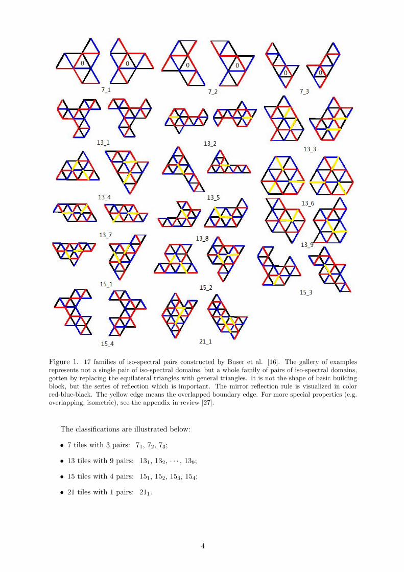
Figure 1. 17 families of iso-spectral pairs constructed by Buser et al. [16]. The gallery of examplesrepresents not a single pair of iso-spectral domains, but a whole family of pairs of iso-spectral domains,gotten by replacing the equilateral triangles with general triangles. It is not the shape of basic buildingblock, but the series of reflection which is important. The mirror reflection rule is visualized in colorred-blue-black. The yellow edge means the overlapped boundary edge. For more special properties (e.g.overlapping, isometric), see the appendix in review [27].

The classifications are illustrated below:

• 7 tiles with 3 pairs: 71, 72, 73;

• 13 tiles with 9 pairs: 131, 132, · · · , 139;

• 15 tiles with 4 pairs: 151, 152, 153, 154;

• 21 tiles with 1 pairs: 211.

4

2 Transplantation method

The transplantation proof was first applied to Riemann surfaces by Buser [11], and to reexamine

iso-spectrality of planar domains given in [16]. Quoting sentence from Buser “We shall show that

the eigenfunctions on the first surface can be suitable transplanted to yield eigenfunctions with

the same eigenvalue on the second surface and vice-versa”, we know suitable transplantation is

important. Berard [15] followed this versatile method to reproof the iso-spectrality of the pair

constructed by Gordon et al.. Okada and Shudo [18] formalised the matrix representation (i.e.

transplantation matrix T ) of transplantation of eigenfunctions. In fact, it turns out that the

matrix T is just the incidence matrix of the graph associated with a certain finite projective

space [25] [26]. Giraud and Thas [27] reviewed the fascinating relation between the iso-spectral

pairs and geometry of vector spaces over finite fields. Illustrating one simple method to obtain

transplantation matrix of the 17 pairs, we follow the definition mentioned in [18, 25, 26, 27],

and describe it with red-blue-black reflection rule.

Figure 2. The special pair of 211: termed as Aye-Aye and Beluga [36]. Each is a polyform composedof 21 identical triangles with angles (30o, 60o, 90o), and created via a specific series of mirror reflections(e.g. basic tile labeled 1 is mirrored to tile 2 by red side). The labels can be arbitrary, for convenience,we keep them consistent with the labels in [36].

Definition 2.1. The transplantation matrix T must be such that

TAν = BνT, ν = 1 (red), 2 (blue), 3 (black). (2.1)

In Equation (2.1), matrices Aν and Bν describe how the tiles are glued togethers (i.e. reflection

rule). For example,

• Aνi,j = 1 if and only if the edge number (color) ν of i glues tile i to tile j;

• Aνi,i = −1 if the edge number ν of i glues nothing (boundary);

• 0, otherwise.

For special pair of 211 depicted in Figure 2 , ν runs form 1 to 3 (red to black). That is also

alternatively corresponding with middle, long and short edge. If you keep the labels of Aye-Aye

and Beluga shape, line i contains a 1 at the column j where i and j are glued by their red

side; Otherwise the red side is the boundary of the tile, line i contains a -1. So for the red side,

the matrix A1 (associated with the Aye-Aye shape) would be that A11,2 = 1, A1

2,1 = 1, A13,3 =

−1, A14,5 = 1, A1

5,4 = 1 and so on. Similarly the B1 matrix would be associate with the Beluga

5

Figure 3. Three iso-spectral pairs following the reflection rule of 73 (e.g. basic tile labeled 1 is mirroredto tile 2 by blue side). (A) This pair is isometric with equilateral triangle as the basic tile. (B) This pair isnon-isometric with (30o, 60o, 90o) triangle as the basic tile. Sleeman and Hua [24] utilized it to constructiso-spectral domains with fractal border. (C) This pair (GWW) is the paradigmatic pair constructed byGordon et al.

shape and yields B11,2 = 1, B1

2,1 = 1, . . . , B16,6 = −1 and so on. Then once you have all matrices

Aν and Bν for the three sides, finding T just amounts to solving a system of equation. If we

keep the notations that T := CijN×N (N represents 7, 13, 15, 21), combining reflection rule

in Figure 3 with definition 2.1, T can be calculated in the following form:

T =

C11 −C13 C13 −C13 −C11 C11 C13

−C13 C11 −C13 C13 C13 −C11 −C11

C13 −C13 C11 −C13 −C11 C13 C11

−C11 C13 −C13 C11 C13 −C13 −C11

C13 −C11 C13 −C11 −C11 C13 C13

−C11 C11 −C11 C13 C13 −C13 −C13

−C13 C13 −C11 C11 C13 −C11 −C13

. (2.2)

C11 and C13 are the two remaining degrees of freedom after solving Equations (2.1). Extracting

C11 and C13 from Equation (2.2), hence T is simplified like this

T = C11T3 + C13T4, C11 6= C13. (2.3)

Tk has only k nonzero entries in each row and each column. In Buser’s words [16], T3 is the

original mapping while T4 is the complementary mapping. Any linear combination like Equation

(2.3) will also be a transplantation mapping. Once C11 is equal to C13, there will be the nodal line

case (i.e. eigenfunctions will vanish, see book [41] for the explaination), in which the “analytical”

solutions appear.

One can show that transplantation is a sufficient condition to guarantee iso-spectrality (if

the matrix T is not merely a permutation matrix, in which case the two domains would just

have the same shape). The underlying idea is that if φ is an eigenfunction of the first domain

6

and φi its restriction to tile i, then one can build an eigenfunction ϕ of the second domain as

ϕi = CN∑j=1

Tijφj , i = 1, 2, . . . , N. (2.4)

C is some normalization factor in Equation (2.4). The smoothness of ϕi can be easily checked on

all reflecting sides and zero boundary conditions of the second domain, if the above conditions

are satisfied. Following this procedure, the two domains discussed will then be iso-spectral, since

the same map transposing eigenfunctions of the second domain onto the first domain will work

as before. For more mathematical proof, please see pp. 8 in review [27]. Simultaneously, you

can also refer Chapman’s paper-folding for the visualization of transplantation.

As previously described, it is not even necessary for the basic tile to be a triangle. Arbitrary

shape with at least three edges will work. We simply choose a triangle with three sides to

represent the three edges, on which we will reflect the shape. Experiments drawn on frames of

arbitrary shapes were conducted by Even and Pieranski [34] using vibrations of smectic films.

Meanwhile, two series of reflections generating from 73 were highly emphasized. Taking the

words of Even and Pieranski, If one broke the reflection rule, the consequences on the spectrum

are drastic. Moon et al. [27] also designed one “Broken Hawk” violating the rule, which led

significantly difference compared with the spectrum of Bilby and Hawk. In summary, specific

reflection rules inherent in the 17 iso-spectral pairs are very important, when associating with

transplantation matrix to transplant eigenfunctions. Although this theorem considers the 2D

case only, the 3D case is similar.

With notations α and β meaning formal parameters, the calculating results of transplantation

matrix for 17 iso-spectral pairs are given below:

• 7 tiles: T = αT3 + βT4, α 6= β;

• 13 tiles: T = αT4 + βT9, α 6= β;

• 15 tiles: T = αT7 + βT8, α 6= β;

• 21 tiles: T = αT5 + βT16, α 6= β.

Remark 2.2. It is easy to obtain similar relations for Neumann boundary conditions by con-

jugating all matrices Aν and Bν in definition 2.1, with a diagonal entry Aνi,i = 1 according to

whether tile i glues nothing (boundary).

3 How to construct the 3D iso-spectral models

In this section, we explain the idea of constructing iso-spectral pairs in 3D space, which also

can be seen as a real extension of the 2D pairs. There are a number of options for selecting

basic tile in 3D space, such as parallelepiped, tetrahedron, etc. Once you have selected the

basic tile (tetrahedron for example), you only need to fix one of its faces (meaning that you just

forget about it) and color the three other faces by red, blue and black. Then you do the mirror

reflection with respect to red, blue and black according to the rule. That will automatically

generate many 3D iso-spectral pairs.

3.1 Extensions of 71 for instance

In order to facilitate the description of this extension, we first discuss the propeller-shaped

example [16], generated from the 71 pair. In both propellers the central triangle labelled “0” has

a distinguishing property: its sides connect the three inward corners of the propeller. Based on

this property, we choose one basic tetrahedron placing the position “0” of Figure 4. Following

7

the same orientation, we only need to perform the series of reflections rule depicted in Figure 4.

It is remarked that the biggest difference between 2D and 3D is that 2D is reflected by edges,

while 3D is reflected by faces. The following steps describe how to build up 3D iso-spectral

models.

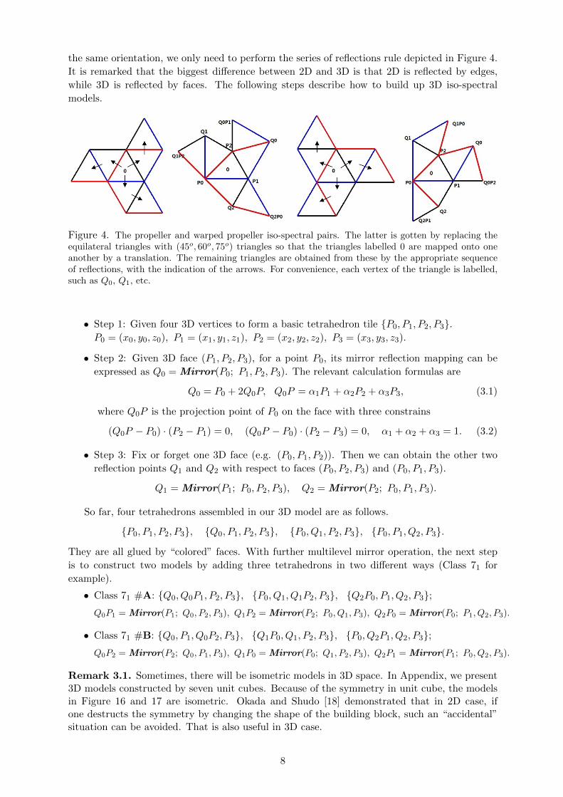
Figure 4. The propeller and warped propeller iso-spectral pairs. The latter is gotten by replacing theequilateral triangles with (45o, 60o, 75o) triangles so that the triangles labelled 0 are mapped onto oneanother by a translation. The remaining triangles are obtained from these by the appropriate sequenceof reflections, with the indication of the arrows. For convenience, each vertex of the triangle is labelled,such as Q0, Q1, etc.

• Step 1: Given four 3D vertices to form a basic tetrahedron tile P0, P1, P2, P3.P0 = (x0, y0, z0), P1 = (x1, y1, z1), P2 = (x2, y2, z2), P3 = (x3, y3, z3).

• Step 2: Given 3D face (P1, P2, P3), for a point P0, its mirror reflection mapping can be

expressed as Q0 = Mirror(P0; P1, P2, P3). The relevant calculation formulas are

Q0 = P0 + 2Q0P, Q0P = α1P1 + α2P2 + α3P3, (3.1)

where Q0P is the projection point of P0 on the face with three constrains

(Q0P − P0) · (P2 − P1) = 0, (Q0P − P0) · (P2 − P3) = 0, α1 + α2 + α3 = 1. (3.2)

• Step 3: Fix or forget one 3D face (e.g. (P0, P1, P2)). Then we can obtain the other two

reflection points Q1 and Q2 with respect to faces (P0, P2, P3) and (P0, P1, P3).

Q1 = Mirror(P1; P0, P2, P3), Q2 = Mirror(P2; P0, P1, P3).

So far, four tetrahedrons assembled in our 3D model are as follows.

P0, P1, P2, P3, Q0, P1, P2, P3, P0, Q1, P2, P3, P0, P1, Q2, P3.

They are all glued by “colored” faces. With further multilevel mirror operation, the next step

is to construct two models by adding three tetrahedrons in two different ways (Class 71 for

example).

• Class 71 #A: Q0, Q0P1, P2, P3, P0, Q1, Q1P2, P3, Q2P0, P1, Q2, P3;Q0P1 = Mirror(P1; Q0, P2, P3), Q1P2 = Mirror(P2; P0, Q1, P3), Q2P0 = Mirror(P0; P1, Q2, P3).

• Class 71 #B: Q0, P1, Q0P2, P3, Q1P0, Q1, P2, P3, P0, Q2P1, Q2, P3;Q0P2 = Mirror(P2; Q0, P1, P3), Q1P0 = Mirror(P0; Q1, P2, P3), Q2P1 = Mirror(P1; P0, Q2, P3).

Remark 3.1. Sometimes, there will be isometric models in 3D space. In Appendix, we present3D models constructed by seven unit cubes. Because of the symmetry in unit cube, the modelsin Figure 16 and 17 are isometric. Okada and Shudo [18] demonstrated that in 2D case, ifone destructs the symmetry by changing the shape of the building block, such an “accidental”situation can be avoided. That is also useful in 3D case.

8

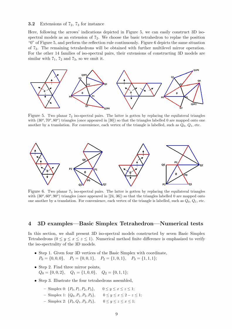
3.2 Extensions of 72, 73 for instance

Here, following the arrows’ indications depicted in Figure 5, we can easily construct 3D iso-spectral models as an extension of 72. We choose the basic tetrahedron to replae the position“0” of Figure 5, and perform the reflection rule continuously. Figure 6 depicts the same situationof 73. The remaining tetrahedrons will be obtained with further multilevel mirror operation.For the other 14 families of iso-spectral pairs, their extensions of constructing 3D models aresimilar with 71, 72 and 73, so we omit it.

Figure 5. Two planar 72 iso-spectral pairs. The latter is gotten by replacing the equilateral triangleswith (30o, 70o, 80o) triangles (once appeared in [30]) so that the triangles labelled 0 are mapped onto oneanother by a translation. For convenience, each vertex of the triangle is labelled, such as Q0, Q1, etc.

Figure 6. Two planar 73 iso-spectral pairs. The latter is gotten by replacing the equilateral triangleswith (30o, 60o, 90o) triangles (once appeared in [24, 36]) so that the triangles labelled 0 are mapped ontoone another by a translation. For convenience, each vertex of the triangle is labelled, such as Q0, Q1, etc.

4 3D examples—Basic Simplex Tetrahedron—Numerical tests

In this section, we shall present 3D iso-spectral models constructed by seven Basic SimplexTetrahedrons (0 ≤ y ≤ x ≤ z ≤ 1). Numerical method finite difference is emphasized to verifythe iso-spectrality of the 3D models.

• Step 1. Given four 3D vertices of the Basic Simplex with coordinate,P0 = 0, 0, 0, P1 = 0, 0, 1, P2 = 1, 0, 1, P3 = 1, 1, 1;

• Step 2. Find three mirror points,Q0 = 0, 0, 2, Q1 = 1, 0, 0, Q2 = 0, 1, 1;

• Step 3. Illustrate the four tetrahedrons assembled,

– Simplex 0: P0, P1, P2, P3, 0 ≤ y ≤ x ≤ z ≤ 1;

– Simplex 1: Q0, P1, P2, P3, 0 ≤ y ≤ x ≤ 2− z ≤ 1;

– Simplex 2: P0, Q1, P2, P3, 0 ≤ y ≤ z ≤ x ≤ 1;

9

Figure 7. Four Simplex Tetrahedrons assembled (termed as kernel Simplex), viewing from different an-gles. Face (P0, P1, P2) is special colored to help us forget it when performing reflection rule. Consequently,faces (Q0, P1, P2), (P0, Q1, P2) and (P0, P1, Q2) are not considered as reflection faces, either.

– Simplex 3: P0, P1, Q2, P3, 0 ≤ x ≤ y ≤ z ≤ 1.

As a foundation of constructing non-isometric 3D models, kernel Simplex (depicted in Fig.7) plays quite an important role, especially for the extension of 71, 72 and 73. Following thereflection rule, we just conduct the multilevel mirror operation on the kernel Simplex, whichis just adding some tetrahedrons. The following step is to classify two non-isometric modelsgenerated from 71.

• Class 71 #A, three mirror points: Q0P1 = 1, 0, 2, Q1P2 = 1, 1, 0, Q2P0 = 0, 0, 2.

– Simplex 4: Q0, Q0P1, P2, P3, 0 ≤ y ≤ 2− z ≤ x ≤ 1;

– Simplex 5: P0, Q1, Q1P2, P3, 0 ≤ z ≤ y ≤ x ≤ 1;

– Simplex 6: Q2P0, P1, Q2, P3, 0 ≤ x ≤ y ≤ 2− z ≤ 1.

• Class 71 #B, three mirror points: Q0P2 = 0, 1, 1, Q1P0 = 2, 0, 0, Q2P1 = 0, 1, 0.

– Simplex 4: Q0, P1, Q0P2, P3, 0 ≤ x ≤ y ≤ 2− z ≤ 1;

– Simplex 5: Q1P0, Q1, P2, P3, 0 ≤ y ≤ z ≤ 2− x ≤ 1;

– Simplex 6: P0, Q2P1, Q2, P3, 0 ≤ x ≤ z ≤ y ≤ 1.

Figure 8. Seven Simplex Tetrahedrons assembled (termed as Class 71 #A), viewing from different angles.The labels in each vertex help us to distinguish the tetrahedrons. The colored tetrahedrons means thethree added tetrahedrons on the Kernel Simplex. Because of the symmetry in Simplex Tetrahedron,points Q0 and Q2P0 coincide.

Remark 4.1. Figure 8 and 9 depict one 3D iso-spectral pair termed as Class 71 #A and Class71 #B respectively. They are all assembled by seven Simplex Tetrahedrons in different ways.Because of the symmetry in the Simplex Tetrahedron, faces (P1, P3, Q0) and (P1, P3, Q2P0)

10

Figure 9. Seven Simplex Tetrahedrons assembled (termed as Class 71 #B), viewing from different angles.The labels in each vertex help us to distinguish the tetrahedrons. The colored tetrahedrons means thethree added tetrahedrons on the Kernel Simplex. Because of the symmetry in Simplex Tetrahedron,points Q2 and Q0P2 coincide.

coincide in Class 71 #A. Similarly, faces (P0, P3, Q2) and (P0, P3, Q0P2) coincide in Class 71#B. For this case, we should also consider these faces as the boundary face.

Remark 4.2. Class 71 #A and Class 71 #B are non-isometric. With the aid of the 3D Printingtechnique, we obtain two models which are obviously non-congruent. Moreover, utilizing theirdistance matrix (the matrix of distances between all vertices), we can also judge they are non-isometric.

In Moorhead’s Ph.D thesis [39], he present 45 shapes to discuss iso-spectrality, using asimple finite difference scheme to calculate eigenvalues. We are also interested in applying finitedifference method to our 3D iso-spectral models. For more detailed results, please see Table 1.That is if we let λk be the approximated k-th eigenvalue for the first Class 71 #A and µk bethe approximated k-th eigenvalue for the second Class 71 #B then

max1≤k≤25

|λk − µk| = 6.2528× 10−13, ‖λk − µk‖L2 = 1.4503× 10−12.

The following step is to classify two non-isometric models generated from 72. You can seethe 3D view in Figure 10 and 11.

• Class 72 #A, three mirror points: Q2P1 = 0, 1, 0, Q1P0 = 2, 0, 0, [Q1P0]P2 = 1, 1, 0.

– Simplex 4: P0, Q2P1, Q2, P3, 0 ≤ x ≤ z ≤ y ≤ 1;

– Simplex 5: Q1P0, Q1, P2, P3, 0 ≤ y ≤ z ≤ 2− x ≤ 1;

– Simplex 6: Q1P0, Q1, [Q1P0]P2, P3, 0 ≤ z ≤ y ≤ 2− x ≤ 1.

• Class 72 #B, three mirror points: Q0P1 = 1, 0, 2, Q1P2 = 1, 1, 0, [Q1P2]P0 = 2, 0, 0.

– Simplex 4: Q0, Q0P1, P2, P3, 0 ≤ y ≤ 2− z ≤ x ≤ 1;

– Simplex 5: P0, Q1, Q1P2, P3, 0 ≤ z ≤ y ≤ x ≤ 1;

– Simplex 6: [Q1P2]P0, Q1, Q1P2, P3, 0 ≤ z ≤ y ≤ 2− x ≤ 1.

Please see Wiki: https://en.wikipedia.org/wiki/3D printing

11

Table 1. The first 25 approximated eigenvalues of the 3D iso-spectral pair: Class 71 #A and Class71 #B, using the simple finite difference method ( please also see [39]) with mesh size h = 1/20. TheDifference refers to the absolute difference between the eigenvalues.

Eigenvalue Class 71 #A Class 71 #B Difference (×10−12)

1 44.4718 44.4718 0.05682 62.8210 62.8210 0.04263 68.9764 68.9764 04 80.4222 80.4222 0.12795 86.0231 86.0231 0.02846 103.2302 103.2302 0.12797 105.6904 105.6904 0.18478 110.1293 110.1293 0.02849 117.5639 117.5639 0.341110 126.6846 126.6846 0.085311 130.2792 130.2792 0.312612 136.1989 136.1989 0.284213 136.5769 136.5769 0.369514 142.5582 142.5582 0.625315 147.9829 147.9829 016 154.1811 154.1811 0.085317 161.1378 161.1378 0.199018 164.5301 164.5301 0.397919 169.0497 169.0497 0.596920 172.1153 172.1153 0.397921 176.0983 176.0983 0.170522 180.6497 180.6497 0.170523 185.0137 185.0137 0.056824 190.4692 190.4692 0.028425 194.8700 194.8700 0.5116

Figure 10. Seven Simplex Tetrahedrons assembled (termed as Class 72 #A), viewing from differentangles. The labels in each vertex help us to distinguish the tetrahedrons. The colored tetrahedronsmeans the three added tetrahedrons on the Kernel Simplex.

12

Figure 11. Seven Simplex Tetrahedrons assembled (termed as Class 72 #B), viewing from differentangles. The labels in each vertex help us to distinguish the tetrahedrons. The colored tetrahedronsmeans the three added tetrahedrons on the Kernel Simplex.

The 3D views in Figure 10 and 11 shows Class 72 #A and 72 #B are non-isometric. Pleasealso see Table 2 for the approximated eigenvalues of this 3D iso-spectral pair. The maximumdifference and L2-norm error are as follows.

max1≤k≤25

|λk − µk| = 0.6821× 10−12, ‖λk − µk‖L2 = 1.4167× 10−12.

Figure 12 shows the GWW prisms which are iso-spectral. They are just constructed from GWWby sweeping the face into a third orthogonal direction for the same distance.

Figure 12. The GWW prisms once appeared in [22][39].

Table 3 shows the detailed results of the first 25 approximated eigenvalues of Class 73 #Aand Class 73 #B. Similarly, we also calculate the maximum difference and L2-norm error.

max1≤k≤25

|λk − µk| = 0.6821× 10−12, ‖λk − µk‖L2 = 1.6766× 10−12.

Figure 13 depicts the 3D X-ray form of Class 73 #A and 73 #B. At the same time, we alsoillustrate other 3D iso-spectral models constructed by Wall Tetrahedrons. Different from theconstruction of Class 73 #A and 73 #B, we fix or forget face (P0, P1, P3) and do multilevel

13

Table 2. The first 25 approximated eigenvalues of the 3D iso-spectral pair: Class 72 #A and Class72 #B, using the simple finite difference method (please also see [39]) with mesh size h = 1/20. TheDifference refers to the absolute difference between the eigenvalues.

Eigenvalue Class 72 #A Class 72 #B Difference (×10−12)

1 44.9835 44.9835 0.11372 61.4888 61.4888 0.12083 70.0240 70.0240 0.38374 80.6794 80.6794 0.17055 86.2937 86.2937 0.27006 102.1243 102.1243 0.19907 104.7903 104.7903 0.07118 110.7750 110.7750 0.18479 121.5084 121.5084 0.241610 124.1022 124.1022 0.127911 129.6075 129.6075 0.682112 136.1989 136.1989 0.056813 137.0019 137.0019 0.142114 142.1820 142.1820 0.284215 146.8989 146.8989 0.085316 157.7060 157.7060 0.284217 160.9049 160.9049 0.369518 163.9460 163.9460 0.142119 165.5862 165.5862 0.341120 171.1039 171.1039 0.369521 178.3842 178.3842 0.397922 183.0443 183.0443 0.454723 185.0180 185.0180 0.113724 191.9694 191.9694 0.227425 195.6234 195.6234 0.0284

Table 3. The first 25 approximated eigenvalues of the 3D iso-spectral pair: Class 73 #A and Class73 #B, using the simple finite difference method ( please also see [39]) with mesh size h = 1/20. TheDifference refers to the absolute difference between the eigenvalues.

Eigenvalue Class 73 #A Class 73 #B Difference (×10−12)

1 49.2289 49.2289 0.02132 56.0467 56.0467 0.02843 72.6396 72.6396 0.18474 79.9743 79.9743 0.11375 92.0586 92.0586 0.18476 99.5111 99.5111 0.38377 104.0452 104.0452 0.22748 113.2988 113.2988 0.29849 120.5720 120.5720 0.113710 124.4357 124.4357 0.554211 131.7220 131.7220 012 133.3562 133.3562 0.341113 136.1989 136.1989 0.369514 144.0266 144.0266 0.454715 152.4877 152.4877 0.170516 156.3340 156.3340 0.113717 156.5645 156.5645 0.056818 162.8653 162.8653 0.397919 169.5866 169.5866 0.085320 173.2912 173.2912 0.369521 179.6543 179.6543 0.085322 185.0656 185.0656 0.397923 186.5775 186.5775 0.426324 190.4249 190.4249 0.113725 193.5350 193.5350 0.6821

14

Figure 13. Seven Simplex Tetrahedrons assembled (termed as Class 73 #A and 73 #B), viewing in 3DX-ray form. Because of symmetry in Simplex Tetrahedron, faces (P1, P3, Q2) and (P1, P3, Q0P2) coincidein Class 73 #A, faces (P1, P3, Q0) and (P1, P3, Q2P2) coincide in Class 73 #B.

mirror reflection following the rule of 73. Given four 3D vertices of the Basic Wall Tetrahedronswith coordinate:

P0 = 0, 0, 0, P1 = 1, 0, 0, P2 = 0, 1, 0, P3 = 0, 0, 1.

We can calculate the mirror points according to Equation (3.1) and Equation (3.2). Figure 14depicts the two 3D iso-spectral models.

Figure 14. Two 3D models assembled by seven Wall Tetrahedrons, viewing in the 3D X-ray form.Generated from 73 by fixing the face (P0, P1, P3), this pair is iso-spectral and non-isometric.

Remark 4.3. For Basic Simplex Tetrahedron (0 ≤ y ≤ x ≤ z ≤ 1) , there exists “analytical”eigenmodes (please refer the explanation of the GWW’s eigenmodes in [30]). The first eigenmodeis expressed in Simplex Tetrahedron of (12 + 22 + 32)π. The first approximated eigenmodes cal-culated by finite difference method are marked in red color, see Table 1-3. Numerical techniquesare therefore employed to approximate such eigenvalues, but even this has its own problems(e.g. the way to deal with reentrant corners).

Remark 4.4. Note that if the colors of faces are permuted the resulting 3D pairs also becomeiso-spectral. For example, the pair 71 represents three distinguishable pairs of models for a fixedtetrahedron.

15

5 Conclusion

Milnor’s work is not a direct answer to the original version of Kac’s question because it isnot concerned with the planar domains. But from Milnor’s example one learned that therereally exists non-congruent domains with the same eigenvalue spectrum. From a mathematicalpoint of view, the spectrum of a drum corresponds to the set of eigenvalues of the negativeLaplacian on a given planar domain, where the solutions vanish at the border (Dirichlet boundaryconditions). Sunada’s idea was to reduce the problem of finding iso-spectral manifolds to a group-theoretical problem, namely, constructing triplets of groups having a certain property. Based onthe Sunada’s method, Buser et al. constructed 17 families of iso-spectral pairs, and confirmedtheir iso-spectrality by the transplantation method. Giraud and Thas reviewed the highlightingmathematical and physical aspects of iso-spectrality.

We revisit the serials of reflection rule inherent in the 17 families of planar iso-spectraldomains. Following the reflection rule visualized by red-blue-black, many 3D iso-spectral modelscan be constructed. Especially for the tetrahedron as the basic building block, we present somevisualized 3D pairs which are iso-spectral and non-isometric. This extension of constructing iso-spectral pairs can also be used in higher dimensions, with transplantation method to guaranteethe respective iso-spectrality.

6 Acknowledgements

This work was supported by the National Science Foundation of China (NSFC 91230109). Thefirst author would like to thank Professor Olivier Giraud for illuminating email indication andwould also like to thank Professor Hua Li, introducing me the software Google SketchUp todraw the 3D Figures.

A Appendix

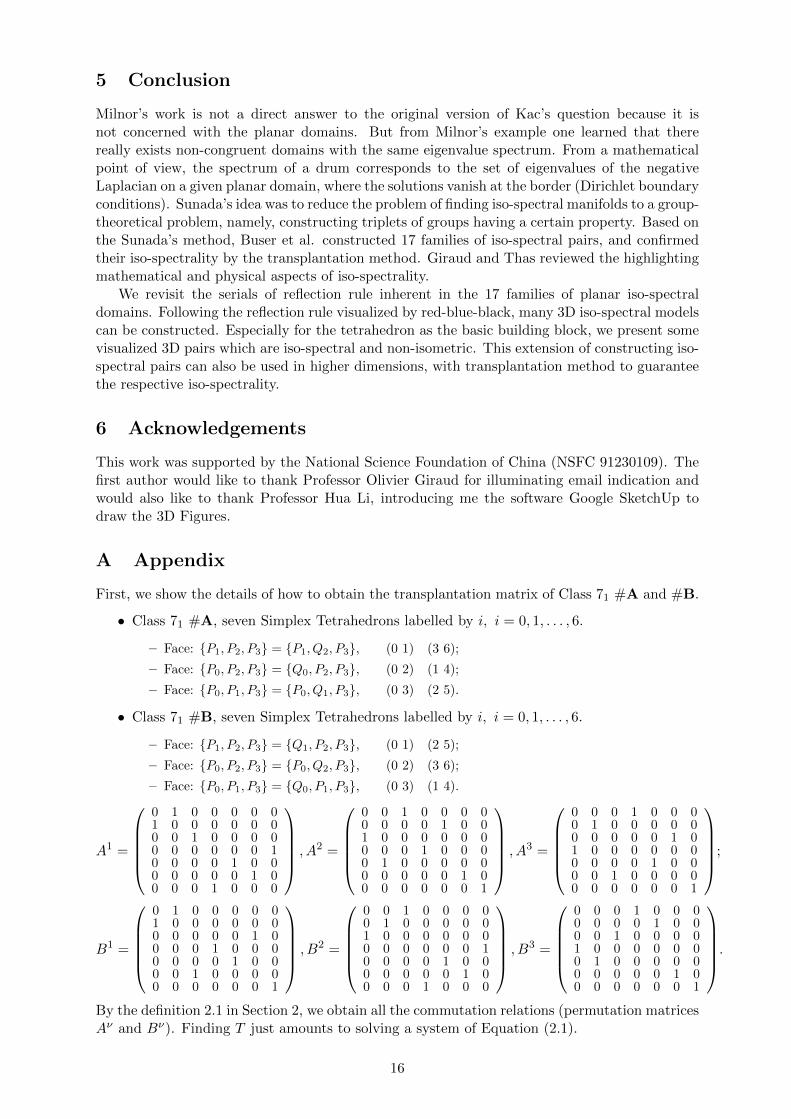
First, we show the details of how to obtain the transplantation matrix of Class 71 #A and #B.

• Class 71 #A, seven Simplex Tetrahedrons labelled by i, i = 0, 1, . . . , 6.

– Face: P1, P2, P3 = P1, Q2, P3, (0 1) (3 6);

– Face: P0, P2, P3 = Q0, P2, P3, (0 2) (1 4);

– Face: P0, P1, P3 = P0, Q1, P3, (0 3) (2 5).

• Class 71 #B, seven Simplex Tetrahedrons labelled by i, i = 0, 1, . . . , 6.

– Face: P1, P2, P3 = Q1, P2, P3, (0 1) (2 5);

– Face: P0, P2, P3 = P0, Q2, P3, (0 2) (3 6);

– Face: P0, P1, P3 = Q0, P1, P3, (0 3) (1 4).

A1 =

0 1 0 0 0 0 01 0 0 0 0 0 00 0 1 0 0 0 00 0 0 0 0 0 10 0 0 0 1 0 00 0 0 0 0 1 00 0 0 1 0 0 0

, A2 =

0 0 1 0 0 0 00 0 0 0 1 0 01 0 0 0 0 0 00 0 0 1 0 0 00 1 0 0 0 0 00 0 0 0 0 1 00 0 0 0 0 0 1

, A3 =

0 0 0 1 0 0 00 1 0 0 0 0 00 0 0 0 0 1 01 0 0 0 0 0 00 0 0 0 1 0 00 0 1 0 0 0 00 0 0 0 0 0 1

;

B1 =

0 1 0 0 0 0 01 0 0 0 0 0 00 0 0 0 0 1 00 0 0 1 0 0 00 0 0 0 1 0 00 0 1 0 0 0 00 0 0 0 0 0 1

, B2 =

0 0 1 0 0 0 00 1 0 0 0 0 01 0 0 0 0 0 00 0 0 0 0 0 10 0 0 0 1 0 00 0 0 0 0 1 00 0 0 1 0 0 0

, B3 =

0 0 0 1 0 0 00 0 0 0 1 0 00 0 1 0 0 0 01 0 0 0 0 0 00 1 0 0 0 0 00 0 0 0 0 1 00 0 0 0 0 0 1

.By the definition 2.1 in Section 2, we obtain all the commutation relations (permutation matricesAν and Bν). Finding T just amounts to solving a system of Equation (2.1).

16

Second,we present two isometric models generated from the Class 71. They are constructedby seven unit cubes depicted in Figure 16 and 17. The gaps between some cubes are to beinterpreted as having zero boundary.

Figure 15. One unit cube and four unit cubes assembled (termed as Kernel Unit Cube). The colors onfaces help us to perform mirror reflection operation.

Figure 16. Seven unit cubes assembled (generated from Class 71 #A), viewing in two angles. The colorson faces help us to perform mirror reflection operation.

Figure 17. Seven unit cubes assembled (generated from Class 71 #B), viewing in two angles. The colorson faces help us to perform mirror reflection operation.

References

[1] M. Kac, Can one hear the shape of a drum? Amer. Math. Monthly 73 (1966) 1-23.

[2] J. Milnor, Eigenvalues of Laplace operator on certain manifolds, Proc. Natl. Acad. Sci. 51(1964) 542.

17

[3] A. Ikeda, On lens spaces which are iso-spectral but not isometric, Ann. Sci. Ecole NormaleSuper. 13 (1980) 303.

[4] M.F. Vigneras, Riemannienes iso-spectrales et non isometrigues, Ann. Math. 112 (1980)21-32.

[5] H. Urakawa, Bounded domains which are iso-spectral but not congruent, Ann. Sci. EcoleNorm. Sup. (1982) 441-456.

[6] M.H. Protter, Can one hear the shape of a drum? Revisited, SIAM Review 29 (1987)185-197.

[7] R. Melrose, Iso-spectral sets of drumheads are compact in C, Math. Sci. Res. Inst. Report(1983) No. 48-83.

[8] B. Osgood, Phillips R and Sarnak P. Compact iso-spectral sets of face domains, Proc. Natl.Acad. Sci. 85 (1988a) 5359-5361.

[9] B. Osgood, Phillips R and Sarnak P. Compact iso-spectral sets of surfaces, J. Funct. Anal.textbf80 (1988b) 212-234.

[10] T. Sunada, Riemannian coverings and iso-spectral manifolds, Ann. of Math. 121 (1985)169-186.

[11] P. Buser, Iso-spectral Riemann surfaces, Ann. Inst. Fourier 36 (1986) 167-192.

[12] C. Gordon, D.L. Webb, S. Wolpert, Iso-spectral face domains and surfaces via Riemannianorbifolds, Invent. Math. 110 (1992a) 1-22.

[13] C. Gordon, D.L. Webb, Iso-spectral convex domains in Euclidean space, Math. ResearchLett. 1 (1994) 539-545.

[14] Gordon C, Webb D L. Iso-spectral convex domains in the hyperbolic face, Proc. Natl. Acad.Sci. 120(3) (1994).

[15] P. Berard, Transplantation et isopectralite, Math. Ann. 292 (1992) 547-559.

[16] P. Buser, J. Conway, P. Doyle, Some planar iso-spectral domains, Int. Math. Res. Notices9 (1994) 391-400.

[17] R. Brooks R, The Sunada method, Comtemp. Math. 231 (1999) 25-35.

[18] Y. Okada, A. Shudo, Equivalence between iso-spectrality and iso-length spectrality for acertain class of planar billiard domains, J. Phys. A: Math. Gen. 34 (2001) 5911-5922.

[19] A. Dhar, D.M. Rao, N. UdayaShankar, S. Sridhar, Iso-spectrality in chaotic billiards, Phys-ical Review 68 (2003) 026208.

[20] H.P.W. Gottlied, Iso-spectral circular membrane. Inverse problems 20(1 (2004) 155.

[21] I.W. Knowles, M.L. McCarthy, Iso-spectral membranes: a connection between shape anddensity, J. Phys. A: Math. Gen. 37 (2004) 8103-8109.

[22] M. Reuter, F.E. Wolter, N. Peinecke, Laplace-Beltrami spectra as Shape-DNA of surfacesand solids, Computer-Aided Design 38 (2006) 342-366.

[23] S.J. Chapman, Drums that sound the same. Amer. Math. Monthly 102(2) (1995) 124-138.

[24] B.D. Sleeman, H. Chen, On nonisometric iso-spectral connected fractal domains, Rev. Mat.Iberoam. 16 (2000) 351-361.

18

[25] O. Giraud, Diffractive orbits in isospectral billiards, J. Phys. A: Math. Gen. 37 (2004)2571-2764.

[26] O. Giraud, Finite geometries and diffractive orbits in iso-spectral billiards, J. Phys. A:Math. Gen. 38 (2005) L477.

[27] O. Giraud, K. Thas, Hearing shapes of drums–mathematical and physical aspects of iso-spectrality. Reviews of modern physics 82(3) (2010) 2213-2255.

[28] H. Wu, D.W.L. Sprung, J. Martorell, Numerical investigation of iso-spectral cavities builtfrom triangles? Phys. Rev. E. 51(1) (1995) 703-708.

[29] S. Scridhar, A. Kudrolli. Experiments on Not Hearing the shape of Drum, Phys. Rev. Lett.72(14) (1995) 2175-2178.

[30] T.A. Driscoll, Eigenmodes of iso-spectral drums, SIAM Rev. 39(1) (1997) 1-17.

[31] J. Descloux, M. Tolley, An accurate algorithm for computing the eigenvalues of a polygonalmembrane, Comput. Methods Appl. Mech. Engrg. 39 (1983) 37-53.

[32] T. Betcke, L.N.Trefethen, Reviving the Method Of particular Solutions, SIAM Rev. 47(3)(2005) 469-491.

[33] L. Fox, P. Henrici, C. Moler C, Approximations and bounds for eigenvalues of ellipticoperators, SIAM J. Numer. Anal. 4(1) (1967) 89-102.

[34] C. Even, P. Pieranski, On “hearing the shape of drums”: An experimental study usingvibrating smectic film, Europhysics Lett. 47(5) (1999) 531-537.

[35] T. A. Driscoll, H. P. W. Gottlieb, Isospectral Shapes with Neumann and Alternating Bound-ary Conditions, Phys. Rev. E. 68 (2003) 016702.

[36] C.R. Moon, L.S. Mattos, B.K. Foster, G. Zeltzer, W. Ko, H.C Manoharan. Quantum phaseextraction in iso-spectral electronic nanostructures, Science 319 (2008) 782-787.

[37] M. Tolea, B. Ostahie, M. Nita, F. Tolea, A. Aldea, Phase extraction in disordered iso-spectral shapes. Phys. Rev. E. 85 (2012) 036604.

[38] P. Amore, One cannot hear the density of a drum (and further aspects of iso-spectrality),Phys. Rev. E. 88(4) (2013) 042915.

[39] S. Moorhead, Can you hear the shape of a cavity? Ph.D. thesis, (2012) University of Oxford.

[40] C. Cox, Iso-spectral Domains in Euclidean 3-Space, Amer. Jour. Under. Res. 11(1) 2012.

[41] R. Courant, D. Hilbert, Methods of mathematical physics. Vol. I. Interscience Publishers,Inc., New York, N.Y., 1953.

19