waves & normal modes - university of oxford · 2 normal modes 5 2.1 the coupled ... before we...
TRANSCRIPT

Waves & Normal Modes
Matt Jarvis
February 2, 2016
Contents
1 Oscillations 2
1.0.1 Simple Harmonic Motion - revision . . . . . . . . . . . . . . . . . . . 2
2 Normal Modes 5
2.1 The coupled pendulum . . . . . . . . . . . . . . . . . . . . . . . . . . . . . . 62.1.1 The Decoupling Method . . . . . . . . . . . . . . . . . . . . . . . . . 72.1.2 The Matrix Method . . . . . . . . . . . . . . . . . . . . . . . . . . . 102.1.3 Initial conditions and examples . . . . . . . . . . . . . . . . . . . . . 132.1.4 Energy of a coupled pendulum . . . . . . . . . . . . . . . . . . . . . 15
2.2 Unequal Coupled Pendula . . . . . . . . . . . . . . . . . . . . . . . . . . . . 182.3 The Horizontal Spring-Mass system . . . . . . . . . . . . . . . . . . . . . . . 22
2.3.1 Decoupling method . . . . . . . . . . . . . . . . . . . . . . . . . . . . 222.3.2 The Matrix Method . . . . . . . . . . . . . . . . . . . . . . . . . . . 232.3.3 Energy of the horizontal spring-mass system . . . . . . . . . . . . . . 252.3.4 Initial Condition . . . . . . . . . . . . . . . . . . . . . . . . . . . . . 26
2.4 Vertical spring-mass system . . . . . . . . . . . . . . . . . . . . . . . . . . . 262.4.1 The matrix method . . . . . . . . . . . . . . . . . . . . . . . . . . . 27
2.5 Interlude: Solving inhomogeneous 2nd order di↵erential equations . . . . . . 282.6 Horizontal spring-mass system with a driving term . . . . . . . . . . . . . . 312.7 The Forced Coupled Pendulum with a Damping Factor . . . . . . . . . . . 33
3 Normal modes II - towards the continuous limit 39
3.1 N -coupled oscillators . . . . . . . . . . . . . . . . . . . . . . . . . . . . . . . 393.1.1 Special cases . . . . . . . . . . . . . . . . . . . . . . . . . . . . . . . 403.1.2 General case . . . . . . . . . . . . . . . . . . . . . . . . . . . . . . . 423.1.3 N very large . . . . . . . . . . . . . . . . . . . . . . . . . . . . . . . 443.1.4 Longitudinal Oscillations . . . . . . . . . . . . . . . . . . . . . . . . 47
4 Waves I 48
4.1 The wave equation . . . . . . . . . . . . . . . . . . . . . . . . . . . . . . . . 484.1.1 The Stretched String . . . . . . . . . . . . . . . . . . . . . . . . . . . 48
4.2 d’Alambert’s solution to the wave equation . . . . . . . . . . . . . . . . . . 504.2.1 Interpretation of d’Alambert’s solution . . . . . . . . . . . . . . . . . 514.2.2 d’Alambert’s solution with boundary conditions . . . . . . . . . . . . 52
4.3 Solving the wave equation by separation of variables . . . . . . . . . . . . . 544.3.1 Negative C . . . . . . . . . . . . . . . . . . . . . . . . . . . . . . . . 55
i

1
4.3.2 Positive C . . . . . . . . . . . . . . . . . . . . . . . . . . . . . . . . . 564.3.3 C=0 . . . . . . . . . . . . . . . . . . . . . . . . . . . . . . . . . . . . 56
4.4 Sinusoidal waves . . . . . . . . . . . . . . . . . . . . . . . . . . . . . . . . . 564.5 Phase Di↵erences . . . . . . . . . . . . . . . . . . . . . . . . . . . . . . . . . 574.6 Energy stored in a mechanical wave . . . . . . . . . . . . . . . . . . . . . . 58
4.6.1 Kinetic Energy . . . . . . . . . . . . . . . . . . . . . . . . . . . . . . 584.6.2 Potential Energy . . . . . . . . . . . . . . . . . . . . . . . . . . . . . 59
5 Waves II 62
5.1 Reflection & Transmission of waves . . . . . . . . . . . . . . . . . . . . . . . 625.1.1 Boundary Conditions . . . . . . . . . . . . . . . . . . . . . . . . . . 635.1.2 Particular cases . . . . . . . . . . . . . . . . . . . . . . . . . . . . . . 64
5.2 Power flow at a boundary . . . . . . . . . . . . . . . . . . . . . . . . . . . . 645.3 Standing Waves . . . . . . . . . . . . . . . . . . . . . . . . . . . . . . . . . . 65

Chapter 1
Oscillations
Before we go into the main body of the course on waves and normal modes, it is useful to
have a small recap on what we know about simple systems where we only have a single
mass on a pendulum for example. This would all come under the remit of simple harmonic
motion, which forms the basis of some of the problems that we will encounter in this course.
1.0.1 Simple Harmonic Motion - revision
First, consider Hooke’s Law,
F = �kx, (1.1)
where F is the force, x is the displacement with respect to the equilibrium position, and k
is the constant of proportionality relating the two.
The usual aim is to solve for x as a function of time t in the oscillation of the spring
or pendulum for example.
We know that F = ma, therefore
F = �kx = m
d
2
x
dt
2
. (1.2)
This equation tells us that we need to find a solution for which the second derivative
is proportional to the negative of itself. We know that functions that obey this are the
sine, cosine and exponentials. So we can try a fairly general solutions of the form,
x(t) = A cos(!t+ �) or x(t) = Ae
i!t (1.3)
2

3
The phase � just provides a linear shift on the time axis, the scale factor ! expands
or contracts the curve on the time axis and the constant A gives the amplitude of the curve.
To check that this all works we can substitute Eq. 1.3 into Eq. 1.2, obtaining
�k [A cos(!t+ �)] = m
⇥�!
2
A cos(!t+ �)⇤
(1.4)
=) (�k +m!
2) [A cos(!t+ �)] = 0 (1.5)
Since this equation must hold at all times, t, we must therefore have,
k �m!
2 = 0 =) ! =
rk
m
. (1.6)
You can also do this slightly more rigourously by writing the di↵erential equation as
�kx = m.
dv
dt
(1.7)
but this is awkward as it contains three variables, x, vv and t. So you can’t use the standard
strategy of separation of variables on the two sides of the equation and then integrate. But
we can write
F = ma = m.
dv
dt
= m.
dx
dt
.
dv
dx
= mv.
dv
dx
. (1.8)
Which then leads to,
F = ma =) � kx = m
✓v
dv
dx
◆=) �
Zkx.dx =
Zmv.dv (1.9)
Integrating, we find
�1
2kx
2 =1
2mv
2 + E, (1.10)
where the constant of integration, E happens to be the energy. It follows that
v = ±r
2
m
rE � 1
2kx
2
, (1.11)
which can be written as,
dx
pE
q1� kx
2
2E
= ±r
2
m
Zdt. (1.12)

4
A trig substitution turns the LHS into an arcsin or arccos function, and the result is
x(t) = A cos(!t+ �) where ! =
rk
m
(1.13)
which is the same result given in Eq. 1.3.
General solutions to Hooke’s law can obviously also encompass combinations of trig
functions and/or exponentials, for example,
x(t) = A sin(!t+ �) (1.14)
x(t) = A sin(!t+ �) = A cos� sin!t+A sin� cos!t (1.15)
therefore,
x(t) = A
1
sin!t+A
2
cos!t (1.16)
is also a solution.
Finally, for the complex exponential solution
x(t) = Ce
i�t (1.17)
F = �kx = Ce
i�t = m
d
2
x
dt
2
= �m�
2
Ce
i�t (1.18)
=) �
2 =k
m
= !
2 (1.19)
=) x(t) = A
0e
i!t +B
0e
�i!t (1.20)
Using Euler’s formula,
e
i✓ = cos ✓ + i sin ✓ (1.21)
x(t) = A
0 cos!t+A
0i sin!t+B
0 cos!t�B
0i sin!t (1.22)
If A = i(A0 �B
0) and B = (A0 +B
0) then
x(t) = A sin!t+B cos!t (1.23)

Chapter 2
Normal Modes
Many physical systems require more than one variable to quantify their configuration; for
example a circuit may have two connected current loops, so one needs to know what current
is flowing in each loop at each moment. Another example is a set of N coupled pendula each
of which is a one-dimensional oscillator. A set of di↵erential equations one for each variable
will determine the dynamics of such a system. For a system of N coupled 1-D oscillators
there exist N normal modes in which all oscillators move with the same frequency and thus
have fixed amplitude ratios (if each oscillator is allowed to move in x�dimensions, then
xN normal modes exist). The normal mode is for whole system. Even though uncoupled
angular frequencies of the oscillators are not the same, the e↵ect of coupling is that all
bodies can move with the same frequency. If the initial state of the system corresponds to
motion in a normal mode then the oscillations continue in the normal mode. However in
general the motion is described by a linear combination of all the normal modes; since the
di↵erential equations are linear such a linear combination is also a solution to the coupled
linear equations.
A normal mode of an oscillating system is the motion in which all parts of the system
move sinusoidally with the same frequency and with a fixed phase relation.
The best way to illustrate the existence and nature of normal modes is to work
through some examples, and to see what kind of motion is produced.
5

6
Figure 2.1: The Coupled Pendulum
2.1 The coupled pendulum
Rather than a single pendulum, now let us consider two pendula which are coupled together
by a spring which is connected to the masses at the end of two thin strings. The spring has
a spring constant of k and the length, l of each string is the same, as shown in Fig. 2.1
Unlike the simple pendulum with a single string and a single mass, we now have to
define the equation of motion of the whole system together. However, we do this in exactly
the same way as we would in any simple pendulum.
We first determine the forces acting on the first mass (left hand side). Like in the
simple pendulum case, we assume that the displacements form the equilibrium positions
are small enough that the restoriing force due to gravity is approximately given by mg tan ✓
and acts along the line of masses. This force related to gravity produces the oscillatory
motions if the pendulum is o↵set from the equilibrium position, i.e.
m
d
2
x
dt
2
= mx = �mg sin ✓x
= �mg
x
l
. (2.1)
Likewise, for the second mass
m
d
2
y
dt
2
= my = �mg sin ✓y
= �mg
y
l
. (2.2)
However, in addition to this gravitational force we also have the force due to the

7
spring that is connected to the masses. This spring introduces additional forces on the two
masses, with the force acting in the opposite direction to the direction of the displacement,
if we assume that the spring obeys Hooke’s law. Therefore, the equations of motion become
modified:
mx = �mg
x
l
� kx+ ky
= �mg
x
l
+ k(y � x),(2.3)
and
my = �mg
y
l
� ky + kx
= �mg
y
l
� k(y � x).(2.4)
We now have two equations and two unknowns. How can we solve these?
2.1.1 The Decoupling Method
The first method is quick and easy, but can only be used in relatively symmetric systems,
e.g. where l and m are the same, as in this case. The underlying strategy of this method is
to combine the equations of motion given in Eqs. 2.3 and 2.4 in ways so that x and y only
appear in unique combinations.
In this problem we can simply try adding the equations of motion, which is one of
the two useful combinations that we will come across.
m(x+ y) = �mg
x
l
+ k(y � x)�mg
y
l
� k(y � x)
= �mg
l
(x+ y)(2.5)
This type of equation should look familiar, where the left-hand side is a second deriva-
tive of the displacement with respect to time, and the right-hand side is a constant multi-
plied by a displacement in x and y. It becomes more clear if we define
q
1
= x+ y and q
1
= x+ = y. (2.6)
Eq. 2.5 then becomes,
mq
1
= �mg
l
q
1
=) q
1
= �g
l
q
1
(2.7)
This is now easily recognisable as the the usual SHM equation, with q
1
= �!
2
q
1
, where

8
Figure 2.2: The centre of mass motion of the coupled pendulum as described by q
1
= x+y.
!
1
=
rg
l
. (2.8)
We can then immediately write a solution for the system as
q
1
= A
1
cos(!1
t+ �
1
), (2.9)
where A
1
and �
1
are arbitrary constants set by the initial or boundary conditions.
The motion described by q
1
= x + y tells us about the coupled motion of the two
pendula in terms of how they oscillate together around a centre of mass. There is no
dependence on the spring whatsoever, as !
1
does not have a term which involves k. This
motion can be visualised as shown in Fig. 2.1.1.
Given what we have learnt, the obvious other combination of x and y is to subtract
Eq. 2.4 from Eq. 2.3:
m(x� y) = �mg
x
l
+ k(y � x) +mg
y
l
+ k(y � x)
= �m
✓g
l
+2k
m
◆(x� y)
(2.10)
Now let us define
q
2
= x� y and q
2
= x� y. (2.11)
This gives us the following,
q
2
= �✓g
l
+2k
m
◆q
2
. (2.12)
We have SHM again, but this time with the q
2
coordinate, i.e. q
2
= �!
2
q
2
, where in this
case

9
Figure 2.3: The relative motion of the coupled pendulum as described by q
2
= x� y.
!
2
=
rg
l
+2k
m
. (2.13)
Again, we can write a solution immediately as
q
2
= A
2
cos(!2
t+ �
2
), (2.14)
with A
2
and �
2
arbitrary constants defined by the initial and boundary conditions.
In this case the q2
represents the relative motion of the coupled pendulum. As should
be clear from the dependence of !2
on the spring constant, this motion must describe how
the motion of the system depends on the compression and expansion of the spring.
The variables q
1
and q
2
are the modes or normal coordinates of the system. In
any normal mode, only one of these coordinates is active at any one time.
It is actually more common to define the normal coordinates with a normalising factor
of 1/p2, such that
q
1
=1p2(x+ y) and q
2
=1p2(x� y). (2.15)
The factor of 1/p2 is chosen to give standard form for the kinetic enery in terms of the
normal modes. We will come to this later.
We now have the two normal modes that describe the system, and the general solution
of the coupled pendulum is just the sum of these two normal modes.
q
1
+ q
2
= x+ y + x� y = 2x

10
which leads to,
x = A
1
cos(!1
t+ �
1
) +A
2
cos(!2
t+ �
2
) (2.16)
and
q
1
� q
2
= x+ y � x+ y = 2y
which leads to,
y = A
1
cos(!1
t+ �
1
)�A
2
cos(!2
t+ �
2
) (2.17)
The constant are then just set by the initial conditions.
2.1.2 The Matrix Method
This method is a bit more involved but in principle it can be used to solve any set up. But
first of all we will use the example of the coupled pendulum shown in Fig. 2.1. One strategy
that we can use is to look for simple kinds of motion where the masses all move with the
same frequency, building up to a general solution by combinig these simple kinds of motion.
So in the matrix method we start by having a guess at the solutions to the system.
By rearranging Eqs. 2.3 and 2.4, we find
mx+mg
l
+ kx� ky = 0
= x+ x
✓g
l
+k
m
◆� k
m
y = 0(2.18)
and similarly,
y + y
✓g
l
+k
m
◆� k
m
x = 0. (2.19)
We can write this as a matrix in the following way,
"d
2
dt
2 +�g
l
+ k
m
�� k
m
� k
m
d
2
dt
2 +�g
l
+ k
m
�#
x
y
�=
00
�. (2.20)

11
Given this equation, we could multiply both sides of the equation by the inverse of
the matrix, which would lead to (x, y) = (0, 0). This is obviously a solution and would
mean that the pendula just hang there and do not move. However, we want to find a
general solution which would involve describing how the masses move, not just when they
are stationary.
We are expecting oscillatory solutions, so let’s just try one, such that
x
y
�= <
X
Y
�e
i!t
, (2.21)
where X and Y are complex constants. Substituting this trial solution into Eq. 2.20 we
find,
�!
2 + g
l
+ k
m
� k
m
� k
m
�!
2 + g
l
+ k
m
� X
Y
�=
00
�. (2.22)
This is the Eigenvector Equation with �!
2 being the eigenvalues.
Therefore we need to find the non-trivial solutions, and the only way to escape the
trivial solution is to ensure that both X and Y must be zero when the inverse of the matrix
does not exist.
To find the inverse of a matrix involves finding cofactors and determinants, which can
be a bit messy. However, the key thing to remember is that
A�1 =1
|A| ⇥CT, (2.23)
where |A| is the determinant of the matrix A and CT is the transposed matrix of the
cofactors.
So determining the inverse of a matrix always involves dividing by the determinant
of that matrix. Therefore, if the determinant is zero then the inverse does not exist. This
is what we want in order to solve Eqn. 2.22. So setting the determinant to zero,
�����!
2 + g
l
+ k
m
� k
m
� k
m
�!
2 + g
l
+ k
m
���� = 0. (2.24)

12
we find the solution to be
✓�!
2 +g
l
+k
m
◆2
�✓
k
m
◆2
= 0 (2.25)
therefore,
✓�!
2 +g
l
+k
m
◆2
�✓
k
m
◆2
= 0
=) �!
2 +g
l
+k
m
= ± k
m
(2.26)
So we get two solutions for !,
!
2
1
=g
l
and !
2
2
=g
l
+2k
m
(2.27)
The ± ambiguity in ! is ignored as you get sinusoidal solutions.
To complete the solution we substitute the values for ! back into the eigenvector
equation.
For !2
1
= g/l, k
m
� k
m
� k
m
k
m
� X
1
Y
1
�=
00
�(2.28)
which leads to X
1
= Y
1
. So (X,Y ) is proportional to the vector (1, 1).
For !2
2
= g/l + 2k/m, � k
m
� k
m
� k
m
� k
m
� X
2
Y
2
�=
00
�(2.29)
which leads to X
2
= �Y
2
. So (X,Y ) is proportional to the vector (1,�1).
We can now write the general solution as the sum of the two solutions that we have
found, x(t)y(t)
�= X
1
11
�e
i!1t +X
2
1�1
�e
i!2t (2.30)
X and Y are complex constants, lets define them as A1
e
i�1 when X = Y , and A
2
e
i�2
when X = �Y . Substituting back into Eq. 2.30, we find
x = A
1
e
i�1e
i!1t +A
2
e
i�2e
i!2t (2.31)

13
y = A
1
e
i�1e
i!1t �A
2
e
i�2e
i!2t (2.32)
Using Euler’s formula (Eq. 1.21) and just considering the real components and re-
moving the imaginary parts,
x = A
1
cos(!1
t+ �
1
) +A
2
cos(!2
t+ �
2
) (2.33)
y = A
1
cos(!1
t+ �
1
)�A
2
cos(!2
t+ �
2
) (2.34)
which are the same normal modes and frequencies that we found from the decoupling
method. These are the general solutions of a coupled pendulum.
The advantage of using the complex exponential is only evident if there is a mixture
of single and double derivatives as in the case of a damped pendulum discussed later. In
the undamped case just discussed it would be equally simple to start with a normal mode
trial solution proportional to cos(!t+ �).
2.1.3 Initial conditions and examples
In this section we will go through an examples using initial conditions, and the motions
that these produce in the coupled pendulum. Further example will be given in the lectures.
Let’s consider the case where, x(t = 0) = a, y(t = 0) = 0 and the initial velocity
of the masses x = (y) = 0. Before we go into the maths, what does this look like? We
know from SHM of a single pendulum that the velocity of the pendulum is zero at its
maximum displacement from equilibrium. But in this case the second pendulum that is
displaced in the y�direction starts at it’s equilibrium position. This must mean that the
spring connecting the two is either stretched or compressed, depending on the definition of
the direction of x and y. It is useful to sketch these initial conditions so that you know
roughly what to expect in terms of the excitation of the normal modes.

14
Using our solutions to the coupled pendulum from Eqs. 2.16 and 2.17, for t = 0 we
get
x(0) = A
1
cos(�1
) +A
2
cos(�2
) = a
y(0) = A
1
cos(�1
)�A
2
cos(�2
) = 0(2.35)
Adding the Eqs. 2.35 together we find 2A1
cos�1
= a, subtracting we find 2A2
cos�2
=
a. So A
1
and A
2
must have non-zero solutions.
We also have information about the initial velocity of the two masses. This therefore
leads us to looking at the first di↵erential of Eqs. 2.16 and 2.17 with respect to time.
x(0) = �A
1
!
1
sin(�1
)�A
2
!
2
sin(�2
) = 0
y(0) = �A
1
!
1
sin(�1
) +A
2
!
2
sin(�2
) = 0(2.36)
Again adding and subtracting Eqs. 2.36, we find A
1
sin�1
= 0 and A
2
sin�2
= 0. As
both A
1
and A
2
have non-zero values, then �
1
= �
2
= 0. Therefore, 2A1
cos�1
= a = 2A1
and 2A2
cos�2
= a = 2A2
, thus A1
= A
2
= a/2.
Substituting these back into Eqs. 2.16 and 2.17, we find
x =a
2(cos!
1
t+ cos!2
t) (2.37)
y =a
2(cos!
1
t� cos!2
t) (2.38)
In this case both normal modes are excited as q1
= (x+ y) 6= 0 and q
2
= (x� y) 6= 0.
As you will see in lectures, we also have cases where only one normal mode is active.
But let us continue with this system and try and see what it is actually doing. We
can rewrite Eqs. 2.37 and 2.38 using some trig identities as,
x = a cos
✓!
1
+ !
2
2t
◆cos
✓!
1
� !
2
2t
◆(2.39)
y = a sin
✓!
1
+ !
2
2t
◆sin
✓!
1
� !
2
2t
◆(2.40)
This shows that we have two distinct frequencies that the system is oscillating in. A
high-frequency mode where the frequency is (!1
+ !
2
)/2 and a low-frequency mode with

15
Figure 2.4: Oscillatory pattern for a system where both normal modes are excited.
(!1
�!
2
)/2. This means that if we were to visualise the oscillations in x and y as a function
of time then we would see a broad envelope defined by the low-frequency term, but within
this enevelope we see much higher frequency oscillations (Fig. 2.1.3).
We can also calculate the period of the oscillations in the usual way. For example the
period od the envelope is
T
env
=2⇡
!
=4⇡
!
1
� !
2
. (2.41)
Here we have a ‘beat’ frequency, where one complete period of the envelope is equal to 2
beats.
‘Beats’ is when energy is transferred between pendula.
2.1.4 Energy of a coupled pendulum
So we have now found the solutions to the coupled pendulum in tersm of how the two
pendula oscillate with time. We can also determine how the energy in the system varies
between di↵erent types of energy, the two main forms of energy being kinetic and potential
energy.
We know that for a perfect system with no friction, then the total energy of the
system is given by the sum of the potential and kinetic energies, U = KE + PE = T + V .

16
The total kinetic energy is given by
T =1
2mx
2 +1
2my
2 (2.42)
and the potential energy comes from two sources in the coupled pendulum, namely the
spring and gravity.
V
spring
=1
2k(y � x)2 (2.43)
V
gravity
= mgh = mg(l � l cos ✓) = lmg(1� cos ✓) (2.44)
Using 2 sin2 ✓ = 1� cos 2✓ and sin ✓ = x/l we find for the x-pendulum
mgh =mgl
2l2x
2 (2.45)
and for the y-pendulum
mgh =mgl
2l2y
2 (2.46)
so that
V
gravity
=mg
2lk(x2 � y
2). (2.47)
Therefore the total potential energy is just the sum of the gravitational and spring
components,
V
total
=1
2m
✓g
l
+k
m
◆(x2 + y
2)� kxy. (2.48)
This is not the only way to find the total energy of the system. We can also use our
knowledge of how the energy is related to the force, and therefore the equations of motion.
We know,
F
X
= �@V
x
@x
and F
y
= �@V
y
@y
, (2.49)
therefore
F
x
= �@V
x
@x
= mx = �mg
x
l
+ k(y � x)
F
y
= �@V
y
@y
= my = �mg
y
l
� k(y � x).(2.50)
Integrating these equations we find,

17
V (x, y) = mg
x
2
2l+
1
2kx
2 � kxy + f(y) + C
V (x, y) = mg
y
2
2l+
1
2ky
2 � kxy + f(x) + C
(2.51)
Neglecting the arbitrary constant C and this just relates to how we define the zero potential,
then we find that the total potential energy is
V
total
=1
2m
✓g
l
+k
m
◆(x2 + y
2)� kxy. (2.52)
as before.
So we have expressions for the kinetic energy and the potential energy, so we can now
write the total energy of the system as
U = T + V =1
2m(x2 + y
2) +1
2
✓g
l
+k
m
◆(x2 + y
2)� kxy (2.53)
but this doesn’t really convey much about what is going on in terms of the energy associated
with each normal mode. So why don’t we go back and rewrite this in terms of the normal
coordinates q1
and q
2
, where we defined
q
1
=1p2(x+ y) and q
2
=1p2(x� y). (2.54)
and found that
!
1
=
rg
l
. and !
2
=
rg
l
+2k
m
. (2.55)
Substituting these into Eq. 2.53, and with a bit of rearranging, we obtain
U =
✓1
2mq
1
2 +1
2m!
2
1
q
2
1
◆+
✓1
2mq
2
2 +1
2m!
2
2
q
2
2
◆. (2.56)
The first term here is then the energy associated with the first normal mode and the second
term is the energy associted with the second normal mode. Therefore the total energy of
the system is simply the sum of the energies in each mode.
So now we have gone through most of the mathematics that we will use when looking
at coupled systems, although we have started with the simplest example. Let us now have
a look ata slightly more complicated system, where the two pendula that are coupled by a
spring are no longer the same.

18
Figure 2.5: The Unequal Coupled Pendulum
2.2 Unequal Coupled Pendula
In Fig. 2.2 we show a system where there are still two pendula coupled by a spring, with
spring constant k, but this time the length of the pendula are di↵erent, with the left-hand
pendulum having length l
1
and the right-hand pendulum having a length of l2
.
This alters the equations of motion and therefore also the solutions to the system. So
the equations of motions of this system are similar to Eqs. 2.3 and 2.4, and are:
mx = �mg
x
l
1
+ k(y � x), (2.57)
and
my = �mg
y
l
2
� k(y � x). (2.58)
Unlike in the previous coupled pendulum, this system is not symmetric. Therefore
let us go straight to the matrix method in order to solve for x and y.
As before, we equate Eqs. 2.57 and 2.58 to zero and write them in a matrix format.
"d
2
dt
2 + g
l1+ k
m
� k
m
� k
m
d
2
dt
2 + g
l2+ k
m
# x
y
�=
00
�(2.59)

19
As before, we define x and y in terms of complex constants and assume an oscillatory
solution of the form e
i!t.
x
y
�= <
X
Y
�e
i!t
, (2.60)
and substituting to form the Eigenfunction equation,"�!
2 + g
l1+ k
m
� k
m
� k
m
�!
2 + g
l2+ k
m
# X
Y
�=
00
�. (2.61)
Again we have the trivial soluton for x = y = 0, but for the non-trivial solutions we
adopt the same process and set the determinant of the matrix to zero, i.e.
������!
2 + g
l1+ k
m
� k
m
� k
m
�!
2 + g
l2+ k
m
����� = 0. (2.62)
Calculating the determinant, we find
✓�!
2 +g
l
1
+k
m
◆✓�!
2 +g
l
2
+k
m
◆�
✓k
m
◆2
= 0 (2.63)
Expanding this and the solving for !2 gives the following,
!
2
1,2
=1
2
2
4(�2
1
+ �
2
2
) +2k
m
±
s
(�2
1
� �
2
2
)2 +
✓2k
m
◆2
3
5 (2.64)
where �
2
1,2
= g
l1,2.
We can check whether this agrees with the previous solution for the equal coupled
pendulum from Section 2.1, by setting l
1
= l
2
= l and checking that we get the same values
for !1
and !
2
that are given in Eq. 2.27.
So now that we have the equations for !
1
and !
2
, we can find x(t) and y(t) in the
usual way, i.e. by substituting Eq. 2.64 into the matrix given in 2.61. Doing this, we find
✓Y
1
X
1
◆
1
=�!
2
1
+ �
2
1
+ (k/m)
k/m
(2.65)
✓X
1
Y
1
◆
2
=�!
2
1
+ �
2
2
+ (k/m)
k/m
(2.66)

20
✓Y
2
X
2
◆
1
=�!
2
2
+ �
2
1
+ (k/m)
k/m
(2.67)
✓X
2
Y
2
◆
2
=�!
2
2
+ �
2
2
+ (k/m)
k/m
(2.68)
Substituting in for !1,2
we find,
✓X
1
Y
1
◆
1
= �2k
m
(�2
2
� �
2
1
) +q
(�2
1
� �
2
2
)2 + (2k/m)2��1
(2.69)
✓X
1
Y
1
◆
2
= �2k
m
(�2
2
� �
2
1
)�q
(�2
1
� �
2
2
)2 + (2k/m)2��1
(2.70)
✓Y
2
X
2
◆
1
= �2k
m
(�2
1
� �
2
2
) +q
(�2
1
� �
2
2
)2 + (2k/m)2��1
(2.71)
✓Y
2
X
2
◆
2
= �2k
m
(�2
1
� �
2
2
)�q
(�2
1
� �
2
2
)2 + (2k/m)2��1
(2.72)
and therefore
✓X
1
Y
1
◆
1
= �1
✓X
2
Y
2
◆
1
(2.73)
similarly, ✓X
1
Y
1
◆
2
= �1
✓X
2
Y
2
◆
2
(2.74)
and we can define this ratio of the amplitudes,
r =
✓Y
2
X
2
◆
1
= �2k
m
(�2
1
� �
2
2
) +q
(�2
1
� �
2
2
)2 + (2k/m)2��1
(2.75)
therefore rX
1
= Y
1
and X
2
= �rY
2
.
We can therefore write the general solution as a function of this amplitude ratio,
x
y
�=
1r
�A
1
cos(!1
t+ �
1
) +
�r
1
�A
2
cos(!2
t+ �
2
) (2.76)

21
Figure 2.6: Oscillatory pattern for the unequal coupled pendulum. Both normal modes areexcited again and a ‘Beats’ solution is apparent but in this case with r < 1 there is anincomplete transfer of energy between the pendula .
So again we can set up some initial conditions and solve for these. As we did in
Sec. 2.1 let us consider x = a; y = 0; x = y = 0, to see what di↵erence the unequal
pendulum length makes.
Without going through all of the maths (which you should try), we find that A
1
=
a/(1 + r
2); A2
= �ra/(1 + r
2); �1
= �
2
= 0.
Hence, substituting these in to the general solution we find
x(t) = a(cos!1
t+ r
2 cos!2
t)/(1 + r
2) (2.77)
y(t) = ar(cos!1
t� cos!2
t)/(1 + r
2) (2.78)
which can be written in terms of the two active frequencies (!1
�!
2
)/2 and (!1
+!
2
)/2
as before. Doing this we get
x(t) = a cos
✓!
1
+ !
2
2t
◆cos
✓!
1
� !
2
2t
◆� a
✓1� r
2
1 + r
2
◆sin
✓!
1
+ !
2
2t
◆sin
✓!
1
� !
2
2t
◆
(2.79)

22
y(t) = �2a
✓r
1 + r
2
◆sin
✓!
1
+ !
2
2t
◆sin
✓!
1
� !
2
2t
◆(2.80)
2.3 The Horizontal Spring-Mass system
We now more away from pendula and consider other systems which produce normal modes.
Here we look at the horizontal spring-mass system (Fig. 2.3) where three spring are con-
necting two masses of mass m to two fixed points at either end.
Figure 2.7: The horizontal spring-mass system.
As usual we first set up the equations of motion:
mu
1
= �↵ku
1
� k(u1
� u
2
) (2.81)
mu
2
= �↵ku
2
+ k(u1
� u
2
) (2.82)
We have what looks like a symmetrical system, so we can probably use the decoupling
method. So let’s use this first and then check that it all looks fine with the matrix method.
2.3.1 Decoupling method
In the decoupling method we define new coordinates which describe the coupled motion
of the two masses, with the usual coordinates being u
1
+ u
2
and u
1
� u
2
, along with a
normalising factor of 1/p2 that ensures that the energies all work out as expected. So as
before, we have
q
1
=1p2(u
1
+ u
2
) and q
2
=1p2(u
1
� u
2
)
q
1
= (u1
+ u
2
) and q
2
= (u1
� u
2
).
(2.83)

23
First, we add Eqs. 2.81 and 2.82,
m(u1
+ u
2
) = mq
1
= �↵k(u1
+ u
2
)� ku
1
+ ku
2
+ ku
1
� ku
2
= �↵k(u1
+ u
2
)(2.84)
=) q
1
=�↵k
m
q
1
(2.85)
Then subtract Eq. 2.82 from 2.81
m(u1
� u
2
) = mq
2
= �↵k(u1
� u
2
)� ku
1
+ ku
2
� ku
1
+ ku
2
= �(↵+ 2)kq2
)(2.86)
=) q
2
= �(↵+ 2)k
m
q
2
(2.87)
We can see that by using the decoupling method we have arrived immediately that
we have two equations that have the usual SHM structure, as such we can easily obtain the
values for omega:
!
2
1
=↵k
m
and !
2
2
=↵+ 2
m
k (2.88)
2.3.2 The Matrix Method
As stated earlier, the matrix method can be used for all systems, not only symmetric
systems so we can check that what we obtain using the decoupling method is in agreement
with an independent method.
So we follow exactly the same process as we did for the coupled pendula, and
1) write out the equations of motion with a homogeneous matrix equation:
"d
2
dt
2 + ↵k
m
+ k
m
� k
m
� k
m
d
2
dt
2 + ↵k
m
+ k
m
# u
1
u
2
�=
00
�. (2.89)
2) Substitute in the trial solution:
u
1
u
2
�= <
X
Y
�e
i!t
. (2.90)
24
�!
2 + ↵k
m
+ k
m
� k
m
� k
m
�!
2 + ↵k
m
+ k
m
� X
Y
�=
00
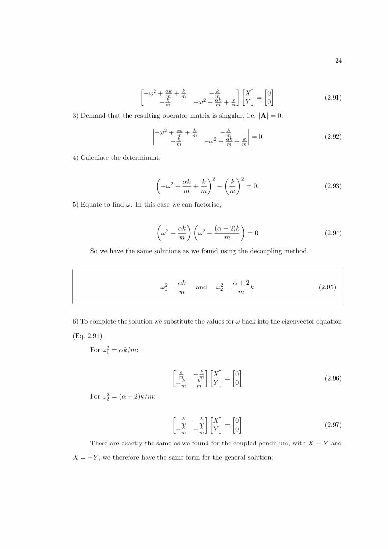
�(2.91)
3) Demand that the resulting operator matrix is singular, i.e. |A| = 0:
�����!
2 + ↵k
m
+ k
m
� k
m
� k
m
�!
2 + ↵k
m
+ k
m
���� = 0 (2.92)
4) Calculate the determinant:
✓�!
2 +↵k
m
+k
m
◆2
�✓
k
m
◆2
= 0, (2.93)
5) Equate to find !. In this case we can factorise,
✓!
2 � ↵k
m
◆✓!
2 � (↵+ 2)k
m
◆= 0 (2.94)
So we have the same solutions as we found using the decoupling method.
!
2
1
=↵k
m
and !
2
2
=↵+ 2
m
k (2.95)
6) To complete the solution we substitute the values for ! back into the eigenvector equation
(Eq. 2.91).
For !2
1
= ↵k/m:
k
m
� k
m
� k
m
k
m
� X
Y
�=
00
�(2.96)
For !2
2
= (↵+ 2)k/m:
� k
m
� k
m
� k
m
� k
m
� X
Y
�=
00
�(2.97)
These are exactly the same as we found for the coupled pendulum, with X = Y and
X = �Y , we therefore have the same form for the general solution:

25
x = A
1
cos(!1
t+ �
1
) +A
2
cos(!2
t+ �
2
) (2.98)
y = A
1
cos(!1
t+ �
1
)�A
2
cos(!2
t+ �
2
) (2.99)
2.3.3 Energy of the horizontal spring-mass system
Unlike in the case of the coupled pendulum, we do not have any gravitational component
to the potential energy, and all energy in this system is contained within the springs. So
let us now just follow through the same method as we used for the coupled pendulum and
determine the total energy of the system.
Again using
q
1
=1p2(u
1
+ u
2
) and q
2
=1p2(u
1
� u
2
).
The total kinetic energy of the system is simply:
K =1
2m(u2
1
+ u
2
2
) =1
2m(q2
1
+ q
2
2
) (2.100)
For the potential energy, we have the component for the two springs at either end
which are fixed to the wall, and a relative displacement term for the middle spring.
V =1
2↵ku
2
1
+1
2k(u
2
� u
1
)2 +1
2↵ku
2
2
(2.101)
Substituting in q
1
and q
2
, we find
V =1
2kq
2
1
+1
2kq
2
2
(↵+ 2) (2.102)
Using the values for !
2
1,2
that we found in the last section !
2
1
= ↵k/m and !
2
2
=
(↵+ 2)k/m:
V =1
2m!
2
1
q
2
1
+1
2m!
2
2
q
2
2
(2.103)

26
Finally, combining the Kinetic Energy and the Potential Energy, we find the total
energy
U =
✓1
2mq
2
1
+1
2m!
2
1
q
2
1
◆+
✓1
2mq
2
2
+1
2m!
2
2
q
2
2
◆(2.104)
Again, the sum of the energies in each normal mode.
2.3.4 Initial Condition
As with the coupled pendulum is is possible to use the general solution to find the motion
of the system given a set of initial conditions. If one were to use the same set of initial
conditions as stated in Sec. 2.1.3 then we also find a similar solution here, i.e.
u
1
= a cos
✓!
1
+ !
2
2t
◆cos
✓!
1
� !
2
2t
◆, (2.105)
u
2
= a sin
✓!
1
+ !
2
2t
◆sin
✓!
1
� !
2
2t
◆, (2.106)
where both normal modes are excited and we have a ‘Beats’ solution, defined by the low-
frequency envelope (!1
� !
2
)/2.
2.4 Vertical spring-mass system
The final ideal oscillating system that we are going to look at is the vertical spring-mass
system (Fig. 2.4).
As usual the first thing that we need to do is to write down the equations of motion.
2mx = �kx� k(x� y) = k(y � 2x) (2.107)
my = �ky + kx = k(x� y) (2.108)
One thing to notice here is that we have unequal masses, this probably means that
the decoupling method is not going to work (try it for yourself). So let us skip straight to
using the matrix method.

27
Figure 2.8: The vertical spring-mass system
2.4.1 The matrix method
Write the equations of motion as a homogeneous matrix equation:
"d
2
dt
2 + k
m
� k
2m
� k
m
d
2
dt
2 + k
m
# x
y
�=
00
�. (2.109)
Substitute in the trial solution
u
1
u
2
�= <
X
Y
�e
i!t
. (2.110)
�!
2 + k
m
� k
2m
� k
m
�!
2 + k
m
� X
Y
�=
00
�(2.111)
Demans that the resulting operator matrix is singular, i.e. |A| = 0 and get the
eigenvalue equation:
✓�!
2 +k
m
◆2
� 1
2
✓k
m
◆2
= 0 (2.112)
From this we can easily show, using the equation to solve a quadratic, that the normal
frequencies !1
and !
2
are
!
2
1,2
=k
m
✓1± 1p
2
◆(2.113)

28
We can now obtain the normal modes of the vertical spring-mass system by substi-
tuting the values for !1,2
in to the eigenvector equation.
✓�!
2
1,2
+k
m
◆X �
✓k
2m
◆Y = 0, (2.114)
For normal mode 1, (!1
) yields, X/Y = �1/p2, and for normal mode 2 (!
2
) yields
X/Y = 1/p2.
We can easily visualise the motion that these two normal modes represent, as they
are again analogous to the couple pendulum, with one representing a centre of mass motion,
where both X and Y are moving in the same direction, or relative motion where they are
moving in opposite directions (Fig. 2.4.1)..
Figure 2.9: The vertical spring-mass system normal modes. On the left-hand side is thecentre of mass motion described by X/Y = 1/
p2 and on the right-hand side is the relative
motion described by X/Y = �1/p2.
2.5 Interlude: Solving inhomogeneous 2nd order di↵erentialequations
In the next section we will tackle a problem which involves dealing with a inhomogeneous
2nd order di↵erential equation, where the simple solution obtained by setting the determi-
nant of the matrix is zero only makes up a part of the general solution. As a precursor to
this, in this section we will go through solving a simple 2nd order di↵erential equation that
is no equal to zero.
Let us consider the problem:
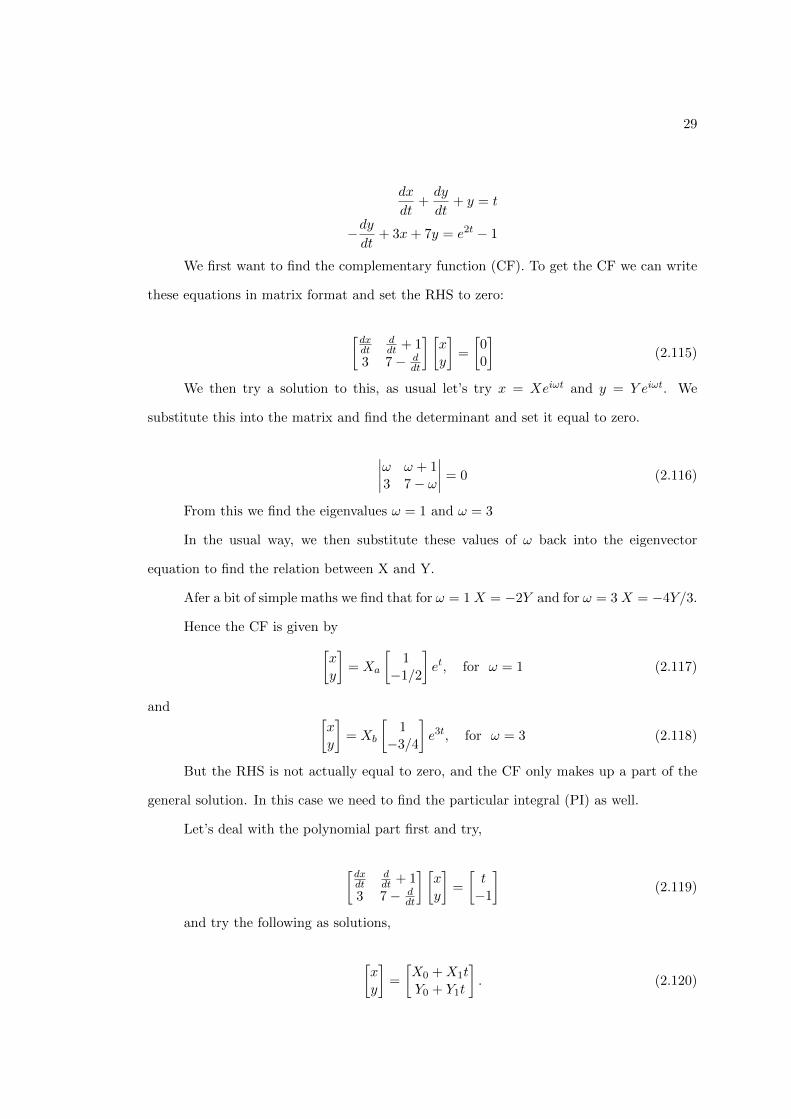
29
dx
dt
+dy
dt
+ y = t
�dy
dt
+ 3x+ 7y = e
2t � 1
We first want to find the complementary function (CF). To get the CF we can write
these equations in matrix format and set the RHS to zero:
dx
dt
d
dt
+ 13 7� d
dt
� x
y
�=
00
�(2.115)
We then try a solution to this, as usual let’s try x = Xe
i!t and y = Y e
i!t. We
substitute this into the matrix and find the determinant and set it equal to zero.
����! ! + 13 7� !
���� = 0 (2.116)
From this we find the eigenvalues ! = 1 and ! = 3
In the usual way, we then substitute these values of ! back into the eigenvector
equation to find the relation between X and Y.
Afer a bit of simple maths we find that for ! = 1X = �2Y and for ! = 3X = �4Y/3.
Hence the CF is given by
x
y
�= X
a
1
�1/2
�e
t
, for ! = 1 (2.117)
and x
y
�= X
b
1
�3/4
�e
3t
, for ! = 3 (2.118)
But the RHS is not actually equal to zero, and the CF only makes up a part of the
general solution. In this case we need to find the particular integral (PI) as well.
Let’s deal with the polynomial part first and try,
dx
dt
d
dt
+ 13 7� d
dt
� x
y
�=
t
�1
�(2.119)
and try the following as solutions,
x
y
�=
X
0
+X
1
t
Y
0
+ Y
1
t
�. (2.120)

30
With this trial solution dx
dt
= X
1
and dy
dt
= Y
1
, therefore substituting these into
Eq. 2.119, we obtain,
X
1
+ Y
1
+ Y
0
+ Y
1
t = t
it therefore follows that Y
1
= 1 and X
1
+ Y
1
+ Y
0
= 0 =) X
1
+ Y
0
= �1 (2.121)
We also have,
3(X0
+X
1
t) + 7(Y0
+ Y
1
t)� Y
1
= �1
it therefore follows that 3X0
+ 7Y0
= 0 and 3X1
+ 7Y1
= 0 =) X
1
= �7
3
(2.122)
Therefore, we have Y
0
= �1 + 7
3
= 4
3
and X
0
= �7
3
Y
0
= �28
9
. We therefore get,
x
y
�=
�28
9
� 7
3
t
4
3
+ t
�(2.123)
Finally, we now have to look at the exponential term. Let’s try,
x
y
�=
X
Y
�e
2t (2.124)
so dx
dt
= 2Xe
2t and dy
dt
= 2Y e
2t.
From this we find the following,
2 2 + 13 7� 2
� X
Y
�=
01
�(2.125)
Therefore,
2X + 3Y = 0 ! X = �3
2
Y
3X + 5Y = 1 ! (�9
2
+ 5)Y = 1 .
So we find that Y = 2 and X = �3..
To find the general solution we just bring all of these together, i.e. CF + PI1
+ PI2
.
x
y
�= X
a
1
�1/2
�e
t +X
b
1
�3/4
�e
3
t+
�32
�e
2t +
�28
9
� 7
3
t
4
3
+ t
�(2.126)
where the first two terms come from the CF and the second two terms comes from
the two PIs.

31
Figure 2.10: The driven horizontal spring.
2.6 Horizontal spring-mass system with a driving term
This brings us on to the penultimate system that we are going to consider in this part of
the course.
Consider two masses moving without friction connected to two springs, of spring
constant 2k and k, with the spring of 2k connected to a wall, which is driven by an external
force to have a time-dependent displacement, given by x(t) = A sin
✓qk
m
t
◆.
The equations of motion are therefore,
mu
1
= 2k[x(t)� u
1
]� k(u1
� u
2
)
mu
2
= k(u1
� u
2
)(2.127)
So as in Sec. 2.5 we first find the complementary function, and consider the homoge-
neous case with x(t) = 0. In this case the equations of motion form the following,
"d
2
dt
2 + 3k
m
� k
m
� k
m
d
2
dt
2 + k
m
# u
1
u
2
�=
00
�(2.128)
Let us try the usual form of a solution,
u
1
u
2
�= <
X
Y
�e
i!t (2.129)
and the equate the determinant of this matrix to zero, and find the eigenvalues.
✓!
2 +3k
m
◆✓�!
2 +k
m
◆� k
2 = 0

32
!
2 =2k
m
± 1
2
s
16
✓k
m
◆2
� 8
✓k
m
◆2
) !
2 =k
m
(2±p2)
Substituting these values for ! back into the eigenvector equation (�!
2+3k/m)X �
kY = 0 we find;
for !2 = (2 +p2)k/m
X(3k � (2 +p2)k) = kY therefore Y = (1 +
p2)X (2.130)
for !2 = (2�p2)k/m
X(3k � (2�p2)k) = kY therefore Y = (1�
p2)X (2.131)
So the ratio of the amplitudes in the CF are
✓Y
X
◆
1
= 1 +p2 and
✓Y
X
◆
2
= 1�p2
Now we have to go back to the original equations of motion and find a solution for
the particular integral. Writing the equations of motion in matrix form, we have
"d
2
dt
2 + 3k
m
� k
m
� k
m
d
2
dt
2 + k
m
# u
1
u
2
�=
Ak
m
20
�<e
i
qk
m
t
�(2.132)
Try the ansatz, u
1
u
2
�= <
✓P
Q
�e
i
qk
m
t
◆(2.133)
from which we find that d2P/dt2 = �k exp[ip
k/mt]/m, therefore we have
� k
m
+ 3k
m
� k
m
� k
m
0
� P
Q
�=
kA
m
20
�(2.134)
This equation is of the form MU = V, rearranging to find U = M�1V. So we need
to calculate the inverse of the matrix M. So to calculate the inverse, we are required to
find the determinant and the transpose of the cofactor matrix (see Eq. 2.23).
The determinant is simply |M| = �( k
m
)2, and the cofactor matrix is

33
adj =
0 k
m
k
m
2k
m
�and therefore M�1 = �
⇣m
k
⌘2
0 k
m
k
m
2k
m
�=
⇣m
k
⌘0 �1�1 �2
�(2.135)
Substituing back into Eq. 2.134 we obtain
P
Q
�=
kA
m
20
�⇣m
k
⌘0 �1�1 �2
�(2.136)
Therefore, P
Q
�=
0
�2A
�(2.137)
So finally we get to the general solution which is the sum of the CF and PI:
u
1
u
2
�= A
1
1
1�p2
�cos
(k
m
(2 +p2)
� 12
t+ �
1
)
+A
2
1
1 +p2
�cos
(k
m
(2�p2)
� 12
t+ �
2
)
+
0
�2A
�cos
rk
m
t
(2.138)
2.7 The Forced Coupled Pendulum with a Damping Factor
Figure 2.11: The Forced Coupled Pendulum. The coupled pendulum in this case has botha driving terms given by F cos↵t and a retarding force �⇥ v, where v is the velocity of themasses.

34
The last example that we will work through in this section of the course, is one in
which we not only have a driving force, but also a damping term. This is therefore more
akin to a real-life system where things are not frictionless. In fact such a system forms of
the basis for many mechanical systems in the real world.
So let us consider the system which is shown in Fig. 2.7. However, in addition to the
gravitational force and the force due to the spring, we also apply a driving force to the x
mass, as denoted by the F cos↵t term, which provides a cyclic pumping motion. We also
consider a damping force acting on both masses, which is related to the velocity of the
masses by F
ret
= �v.
As before we set up the equations of motion.
mx = �x� mg
l
x+ k(y � x) + F cos↵t (2.139)
my = �y � mg
l
y + k(y � x) (2.140)
These are exactly the same equations of motion as foind for the coupled pendulum
as you would expect, but with the additional terms due to the damping force (in both
expressions) and the driving force (in the expression for the x motion).
This looks like a non-trivial problem, so let us go straight to using the matrix method.
So the general matrix for the equations of motion is given by
"d
2
dt
2 + g
l
+ k
m
+ �
m
d
dt
� k
m
� k
m
d
2
dt
2 + g
l
+ k
m
+ �
m
d
dt
# x
y
�=
F
m
10
�<(ei↵t) (2.141)
We use the fact that cos↵t = <(ei↵t) here, but you will obtain the same solution if you use
cos↵t.
The right-hand side is not equal to zero, so this is an inhomogeneous matrix as we
could infer directly from the equations of motion. Therefore, we need to find the solution to
the homogeneous equivalent (the complementary function; CF), and the particular integral.
To find the CF, we write down the homogeneous equations and solve as before;

35
"d
2
dt
2 + g
l
+ k
m
+ �
m
d
dt
� k
m
� k
m
d
2
dt
2 + g
l
+ k
m
+ �
m
d
dt
# x
y
�=
00
�(2.142)
Try the following, x
y
�= <
X
Y
�e
i!t (2.143)
so that
dx
dt
= i!Xe
i!t andd
2
x
dt
2
= �!
2
Xe
i!t
dy
dt
= i!Y e
i!t andd
2
y
dt
2
= �!
2
Y e
i!t
and find the eigenvalues from the following determinant,
�����!
2 + g
l
+ k
m
+ �
m
i! � k
m
� k
m
�!
2 + g
l
+ k
m
+ �
m
i!
���� = 0, (2.144)
which leads to,
✓�!
2 + i!
�
m
+g
l
+k
m
◆2
�✓
k
m
◆2
= 0
=)✓�!
2 + i!
�
m
+g
l
+k
m
◆= ±
✓k
m
◆ (2.145)
Solve using the equations for solving a quadratic for both ±(k/m).
For +(k/m),
!
1
=i�
2m±
rg
l
�⇣
�
2m
⌘2
(2.146)
For �(k/m),
!
1
=i�
2m±
s✓g
l
+2k
m
◆�
⇣�
2m
⌘2
(2.147)
You should notice that these are similar to the eigenvalues in the simple coupled
pendulum case, where !
2
1
= g/l and !
2
= g/l + 2k/m (Eq. 2.27). We have the same terms
for this system, as you might expect, but also the additional terms that include the damping
factor.
So we can rewrite these in terms of these original values for !1,2
as,
!
1,2
=i�
2m±
r!
2
1,2
�⇣
�
2m
⌘2
. (2.148)

36
There is no physical di↵erence between the ± variants here, so from now on we will just
use the positive solution.
We substitute these eigenvalues into the eigenvector equation to find the ratio of the
amplitudes in each normal mode, and thus find the CF. With a bit of simple maths, for !1
,
we find X = Y and for !2
we find X = �Y .
Remembering Eq. 2.143,
x = <(Xe
i!1,2t) and y = <(Y e
i!1,2t)
we find that,
x
y
�= e
(� �t
2m)
(A
1
11
�cos
"✓!
2
1
�⇣
�
2m
⌘2
◆ 12
t+ �
1
#+A
2
1�1
�cos
"✓!
2
2
�⇣
�
2m
⌘2
◆ 12
t+ �
2
#)
(2.149)
where !
1
= g/l and !
2
= g/l + 2k/m. As we might expect, we introduce an exponential
decay factor, which describes the damping force acting on the two masses.
As a note, you can solve this part with the decoupling method and then using a trial
solution of the form q = <(ei!t) and you get the same results.
However, to obtain the general solution, which includes the driving force term, we
need to calculate the PI as well.
Starting from Eqn. 2.141, we now try the ansatz,
x
y
�= <
⇢P
Q
�e
i↵t
�(2.150)
which requires us to solve a matrix of the form MU = V, as we did in Sec. 2.6, so
we rearrange to find U = M�1V.
Therefore we have,
P
Q
�= M�1
F
m
10
�(2.151)
and use Eq. 2.23 to find M�1.
So we first find the determinant of M,
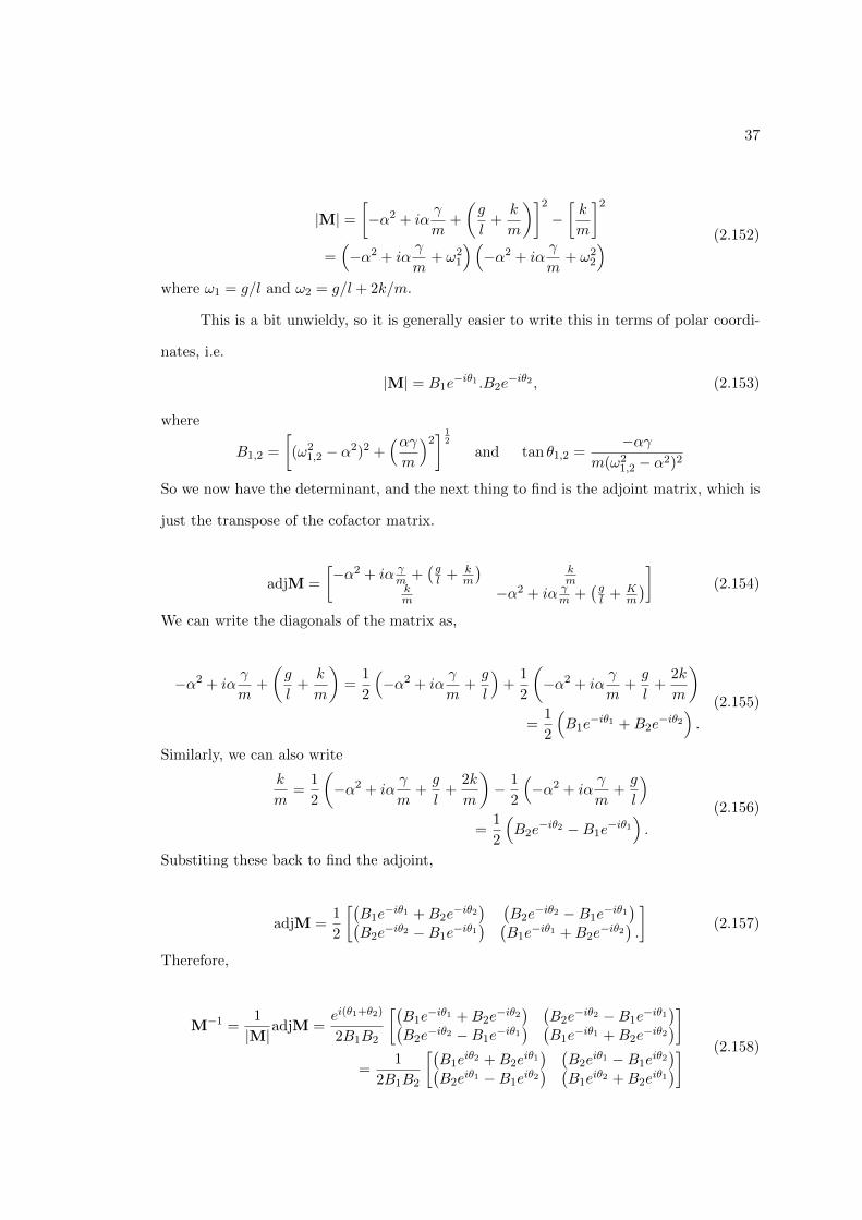
37
|M| =�↵
2 + i↵
�
m
+
✓g
l
+k
m
◆�2
�k
m
�2
=⇣�↵
2 + i↵
�
m
+ !
2
1
⌘⇣�↵
2 + i↵
�
m
+ !
2
2
⌘ (2.152)
where !
1
= g/l and !
2
= g/l + 2k/m.
This is a bit unwieldy, so it is generally easier to write this in terms of polar coordi-
nates, i.e.
|M| = B
1
e
�i✓1.B
2
e
�i✓2, (2.153)
where
B
1,2
=
(!2
1,2
� ↵
2)2 +⇣↵�
m
⌘2
� 12
and tan ✓1,2
=�↵�
m(!2
1,2
� ↵
2)2
So we now have the determinant, and the next thing to find is the adjoint matrix, which is
just the transpose of the cofactor matrix.
adjM =
�↵
2 + i↵
�
m
+�g
l
+ k
m
�k
m
k
m
�↵
2 + i↵
�
m
+�g
l
+ K
m
��
(2.154)
We can write the diagonals of the matrix as,
�↵
2 + i↵
�
m
+
✓g
l
+k
m
◆=
1
2
⇣�↵
2 + i↵
�
m
+g
l
⌘+
1
2
✓�↵
2 + i↵
�
m
+g
l
+2k
m
◆
=1
2
⇣B
1
e
�i✓1 +B
2
e
�i✓2
⌘.
(2.155)
Similarly, we can also write
k
m
=1
2
✓�↵
2 + i↵
�
m
+g
l
+2k
m
◆� 1
2
⇣�↵
2 + i↵
�
m
+g
l
⌘
=1
2
⇣B
2
e
�i✓2 �B
1
e
�i✓1
⌘.
(2.156)
Substiting these back to find the adjoint,
adjM =1
2
�B
1
e
�i✓1 +B
2
e
�i✓2� �
B
2
e
�i✓2 �B
1
e
�i✓1�
�B
2
e
�i✓2 �B
1
e
�i✓1� �
B
1
e
�i✓1 +B
2
e
�i✓2�.
�(2.157)
Therefore,
M�1 =1
|M|adjM =e
i(✓1+✓2)
2B1
B
2
�B
1
e
�i✓1 +B
2
e
�i✓2� �
B
2
e
�i✓2 �B
1
e
�i✓1�
�B
2
e
�i✓2 �B
1
e
�i✓1� �
B
1
e
�i✓1 +B
2
e
�i✓2��
=1
2B1
B
2
�B
1
e
i✓2 +B
2
e
i✓1� �
B
2
e
i✓1 �B
1
e
i✓2�
�B
2
e
i✓1 �B
1
e
i✓2� �
B
1
e
i✓2 +B
2
e
i✓1�� (2.158)

38
Recall, x
y
�=
F
m
<✓M�1
10
�e
i↵t
◆, (2.159)
therefore x
y
�=
F
2mB
1
B
2
B
1
cos(↵t+ ✓
2
) +B
2
cos(↵t+ ✓
1
)B
2
cos(↵t+ ✓
1
)�B
1
cos(↵t+ ✓
2
)
�(2.160)
with
B
1,2
=
(!2
1,2
� ↵
2)2 +⇣↵�
m
⌘2
� 12
and tan ✓1,2
=�↵�
m(!2
1,2
� ↵
2)2
So finally, the general solution is the sum of the CF and the PI;
x
y
�= e
(� �t
2m)
(A
1
11
�cos
"✓!
2
1
�⇣
�
2m
⌘2
◆ 12
t+ �
1
#)
+e
(� �t
2m)
(A
2
1�1
�cos
"✓!
2
2
�⇣
�
2m
⌘2
◆ 12
t+ �
2
#)
+F
2mB
1
B
2
B
1
cos(↵t+ ✓
2
) +B
2
cos(↵t+ ✓
1
)B
2
cos(↵t+ ✓
1
)�B
1
cos(↵t+ ✓
2
)
�.
(2.161)
The complementary function is the “transient” solution determined by the external
conditions, whereas the particular integral gives the “steady state” solution determined by
the driving force.

Chapter 3
Normal modes II - towards thecontinuous limit
In the last few sections we have built up the foundations for the study of waves in general.
For the remainder of the course we will be focusing on various types of wave, and the general
applicability of the equations which govern waves across many parts of physics.
We will look at two general forms of waves; first we will consider the non-dispersive
system, which means that the speed at which the wav travels is not dependent on the
wavelength and frequency. Later one we will look at dispersive waves, where the speed at
which the wave travels does depend on the frequency, this leads to the introduction of group
velocity.
3.1 N-coupled oscillators
From our work looking at normal modes, we know that we can describe a system of coupled
oscillators by the linear superposition ofN normal modes, whereN in the coupled pendulum
case was the number of masses on pendula for example.
In this section we will look what happens when we extend this superposition to the
continuous limit, i.e. for a single piece of wire or string. Rather than individual masses
here, we would have a string that you could consider as being the summation of very small
bits of string of length dl and a mass that relates to these very small parts of the string.
Fig. 3.1.2 shows a diagram of a stretched string, where we split the string up into
small mass elements. In this example, we assume that all of the angles of the stretched
39

40
Figure 3.1: A simple string that has been stretched by a very small amount at its centre.
string from the horizontal are small.
As before, we write down the equations of motion for each element of the string:
In the vertical direction we have,
F
p
y
= my
p
= �T sin↵p�1
+ T sin↵p
(3.1)
For the horizontal direction we have
F
p
x
= �T cos↵p�1
+ T cos↵p
. (3.2)
As we assume ↵ is small, then sin↵i
⇡ tan↵i
⇡ ↵
i
. We can also assume, cos↵i
⇡
1� ↵
2i
2
, using the trig identities cos2 ✓ + sin2 ✓ = 1 and cos 2✓ = cos2 ✓ � sin2 ✓.
Therefore, in the horizontal direction we have zero net force as ↵
p�1
⇡ ↵
p
, as we
would expect if we only stretch the string in the vertical direction at its centre.
For the vertical direction, Eq. 3.1 becomes
F
p
= my
p
= �T
l
(yp
� y
p�1
) +T
l
(yp+1
� y
p
). (3.3)
If we define !
2
0
= T/ml then this becomes
y
p
+ 2!2
0
y
p
� !
2
0
(yp+1
� y
p�1
) = 0. (3.4)
3.1.1 Special cases
Before we move on to the general solution to this equation, let us first look at a few specific,
special cases. Namely, the most simple ones with N = 1 and N = 2.

41
So if we have N = 1 then the stretch string just looks like the system shown in
Fig. 3.1.1.
Figure 3.2: A stretched string with N = 1.
Eq.3.4 becomes
y
1
+ 2!2
0
y
1
= 0, (3.5)
as y
p+1
= y
p�1
in this case, and the equation is the usual form for SHM, i.e. acceleration
proportional to the displacement. Therefore, we can immediately show that the angular
frequency of the oscillation
! =p2!
0
with !
2
0
=T
ml
for N = 1
Now let us look at the N = 2 case. By just drawing what the possibilties are in this
case (Fig. 3.1.1), we know that we should have two solutions.
Figure 3.3: Two possibilities for the starting points for a stretched string with N = 2.Obviously you can have the inverse of these but that is just the same as inverting thedirection of y.
Writing 3.4 for N = 2 we get,
y
1
+ 2!2
0
y
1
� !
2
0
y
2
= 0
y
2
+ 2!2
0
y
2
� !
2
0
y
1
= 0.(3.6)
Let us define the normal coordinates, as we did in Sec. 2.1, i.e.
q
1
=1p2(y
1
+ y
2
) and q
2
=1p2(y
1
� y
2
)

42
which lead to,
q
1
+ !
2
0
q
1
= 0 therefore ! = !
0
q
2
+ 3!2
0
q
2
= 0 therefore ! =p3!
0
.
Therefore, we have two possible normal modes, as you would expect for N = 2. This
is simply analagous to the coupled pendula and N -spring systems that we looked at in
previous lectures.
So now that we have discussed these two special cases, let us move on an try to find
a general solution to the system, where N can be anything.
3.1.2 General case
From Eq. 3.4 we have
y
p
+ 2!2
0
y
p
� !
2
0
(yp+1
� y
p�1
) = 0.
This is a second order di↵erential equation and we expect an oscillatory solution, so
let us consider a solution of the form y
p
= A
p
cos!t.
Note that here we have not included a phase o↵set term, which we represented by �
in previous lectures. By omitting this term here we are just imposing the fact that all the
masses start at rest. Obviously we could reintroduce this terms later.
So substituting the trial solution into Eq. 3.4 gives N equations:
(�!
2 + 2!2
0
)Ap
� !
2
0
(Ap+1
�A
p�1
) = 0 with p = 1, 2, 3...., N
=) A
p+1
+A
p�1
A
p
=�!
2 + 2!2
0
!
2
0
(3.7)
But we know that since ! is the same for all masses, i.e. it doesn’t matter where we
are on the string, then the right-hand side cannot depend on p. So if the RHS does not
depend on p, neither can the left hand side. We also know that if the string is fixed at both
ends, then for p = 0 and p = N + 1, Ap
= 0.
So we need to look for forms of Ap
which satisfy these criteria.
Let us try a description of Ap
of the form, Ap
= C sin p✓, so the left-hand side of
Eq. 3.7 becomes,

43
A
p+1
+A
p�1
A
p
=C [sin(p+ 1)✓ + sin(p� 1)✓]
C sin(p✓)=
2C sin(p✓) cos ✓
C sin(p✓)= 2 cos ✓, (3.8)
which satisfies the criteria for the equation to be independent of p.
Now for the second criteria of when p = 0 or p = N + 1, then A
p
= 0, we just have
to require that (N + 1)✓ = n⇡.
So combining all of this we have
A
p
= C sin
✓pn⇡
N + 1
◆(3.9)
Substituting this back into Eq. 3.7,
!
2 = 2!2
0
1� cos
✓n⇡
N + 1
◆�
=) ! = 2!0
sin
✓n⇡
2(N + 1)
◆ (3.10)
So now we can write the general solution for the displacement in y. Combining Eq. 3.4
with Eq. 3.10 and reintroducing the phase o↵set such that yp
A
p
cos(!t+ �
p
), we obtain
y
pn
(t) = C
n
sin
✓pn⇡
N + 1
◆cos(!
n
t+ �
n
) with !
n
= 2!0
sin
✓n⇡
2(N + 1)
◆(3.11)
where !
0
=
rT
ml
Although the value of n can be greater than N , this would just generate duplicate
solutions, and there are always N normal modes in total. Fig. 3.1.2 shows the 5 normal
modes for the case of N = 5. One thing to note is that all the masses are displaced in such
a way that they fall on an underlying sine curve, as you would expect given the solution
that we have just found.
44
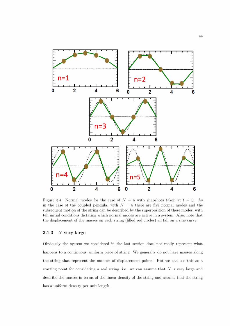
Figure 3.4: Normal modes for the case of N = 5 with snapshots taken at t = 0. Asin the case of the coupled pendula, with N = 5 there are five normal modes and thesubsequent motion of the string can be described by the superposition of these modes, withteh initial conditions dictating which normal modes are active in a system. Also, note thatthe displacement of the masses on each string (filled red circles) all fall on a sine curve.
3.1.3 N very large
Obviously the system we considered in the last section does not really represent what
happens to a continuous, uniform piece of string. We generally do not have masses along
the string that represent the number of displacement points. But we can use this as a
starting point for considering a real string, i.e. we can assume that N is very large and
describe the masses in terms of the linear density of the string and assume that the string
has a uniform density per unit length.

45
So let us consider a string-mass system which has a length L and a total mass M .
We can consider this string as being made up of a series of small elements of length l and
mass m, such that
L = (N + 1)l and M = Nm, and define the linear density of the string as ⇢ = m/l.
Eq. 3.10 describes how the frequency of the oscillation for each normal mode. If we
just consider the mode numbers n which are small in comparison to N , which would be the
case of N is very large as we are assuming, then we essentially remove the sine dependence
and find,
!
n
= 2!0
sin
✓n⇡
2(N + 1)
◆= 2
rT
ml
sin
✓n⇡
2(N + 1)
◆
=) !
n
⇡ 2
sT
m/l
✓n⇡
2(N + 1)l
◆.
(3.12)
As we have defined the linear density above, this then becomes,
!
n
=n⇡
L
sT
⇢
.
(3.13)
This means that all of the normal frequencies are integer multiples of the lowest
frequency given when n = 1, i.e.
!
1
=⇡
L
sT
⇢
.
So we now know that the normal frequencies are just given my integer multiples of
the lowest frequency mode. We now consider the displacement of the string for the same
limit of n small compared to N . Starting from Eq. 3.11, we have
y
pn
(t) = C
n
sin
✓pn⇡
N + 1
◆cos(!
n
t+ �
n
),
but as the elements of the string, each of length l, become smaller and smaller, we approach
a continuous variable along the x�axis, which we define as x = pl, such that
y
n
(x, t) = C
n
sin⇣xn⇡
L
⌘cos(!
n
t+ �
n
), (3.14)
46
resulting in a sinusoidal wave in both x and t, i.e. we have derived the equation for the
complete motion of the string, at least for when n << N . From this we can calculate the
vertical (y) displacement of the string at and time t and at any point along the axis of the
string x.
Let us now look what happens when we move to n = N . From Eq. 3.13 we know
that this must give us the highest frequency mode of the oscillations,
!
N
= 2!0
sin
✓n⇡
2(N + 1)
◆⇡ 2!
0
(3.15)
If we now consider the ratio of the displacements of successive elements of the string
for the n = N mode using Eq. 3.11, i.e.
y
p
y
p+1
=sin
⇣pN⇡
N+1
⌘
sin⇣(p+1)N⇡
N+1
⌘ ⇡ sin(p⇡)
sin(p⇡ + ⇡)⇡ �1. (3.16)
So everything successive element is approximately displaced equally but in the opposite
direction to the previous element. If we lost the approximations, and calculated a more
rigourous solution then what we would find is that we obtain adjacent positive and negative
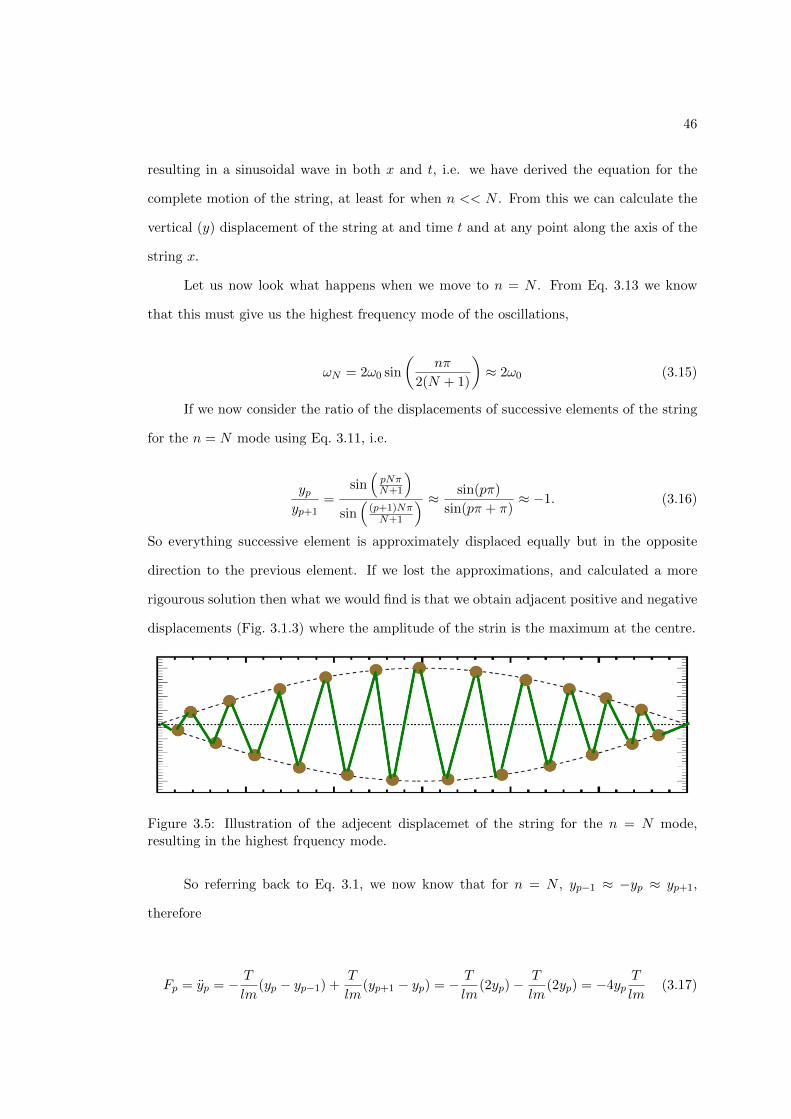
displacements (Fig. 3.1.3) where the amplitude of the strin is the maximum at the centre.
Figure 3.5: Illustration of the adjecent displacemet of the string for the n = N mode,resulting in the highest frquency mode.
So referring back to Eq. 3.1, we now know that for n = N , yp�1
⇡ �y
p
⇡ y
p+1
,
therefore
F
p
= y
p
= � T
lm
(yp
� y
p�1
) +T
lm
(yp+1
� y
p
) = � T
lm
(2yp
)� T
lm
(2yp
) = �4yp
T
lm
(3.17)

47
We defined !
0
= T/ml, therefore y ⇡ �4y!2
0
, from which we find the result !N
⇡ 2!0
.
3.1.4 Longitudinal Oscillations
In the previous section we considered only transverse motion of a string. Obviously waves
can also exist as longitudinal waves, e.g. sound waves and oscillations on a spring. Here
we will quickly demonstrate that the same equations that we found in the previous section
also hold for longitudinal waves.
So rather than the string with N -mass elements, let us consider a horizontal spring
system with N masses between similar springs with spring constant k (Fig. 3.1.4).
Figure 3.6: Horizontal spring-mass system with N -masses.
If up
is the displacement from equilibrium of mass p, then the equation of motions of
each mass is given by,
mu
p
= k(up+1
� u
p
) + k(up�1
� u
p
)
=) u
p
+ 2!2
0
u
p
� !
2
0
(up+1
+ u
p�1
) = 0 with !
2
0
=k
m
.
(3.18)
This is exactly the same form as the equation of motion as given in Eq. 3.4 for the transerve
oscillations of a string made up of N masses. Therefore, the solutions will be exactly the
same.