normal modes and waves
TRANSCRIPT

Chapter 9
Normal Modes and Waves
c©2000 by Harvey Gould and Jan Tobochnik6 December 2000
We discuss the physics of wave phenomena and the motivation and use of Fourier transforms.
9.1 Coupled Oscillators and Normal Modes
Terms such as period, amplitude, and frequency are used to describe both waves and oscillatorymotion. To understand the relation between the latter two phenomena, consider a flexible ropethat is under tension with one end fixed. If we flip the free end, a pulse propagates along therope with a speed that depends on the tension and on the inertial properties of the rope. Atthe macroscopic level, we observe a transverse wave that moves along the length of the rope.In contrast, at the microscopic level we see discrete particles undergoing oscillatory motion in adirection perpendicular to the motion of the wave. One goal of this chapter is to use simulationsto understand the relation between the microscopic dynamics of a simple mechanical model andthe macroscopic wave motion that the model can support. For simplicity, we consider a one-dimensional chain of L particles each of mass M . The particles are coupled by massless springswith force constant K. The equilibrium separation between the particles is a. We denote thedisplacement of particle j from its equilibrium position at time t by uj(t) (see Figure ??). Formany purposes the most realistic boundary conditions are to attach particles j = 1 and j = L tosprings which are attached to fixed walls. We denote the walls by j = 0 and j = L+1, and requirethat u0(t) = uL+1(t) = 0.
The force on an individual particle is determined by the compression or extension of theadjacent springs. The equation of motion of particle j is given by
Md2uj(t)dt2
= −K[uj(t) − uj+1(t)
]−K
[uj(t) − uj−1(t)
]= −K
[2uj(t) − uj+1(t) − uj−1(t)
]. (9.1)
269

CHAPTER 9. NORMAL MODES AND WAVES 270
a
0
a
1
a
2 3 L + 1
u1 u2 u3
Figure 9.1: A one-dimensional chain of L particles of mass M coupled by massless springs withforce constant K. The first and last particles (0 and L + 1) are attached to fixed walls. The topchain shows the oscillators in equilibrium. The bottom chain shows the oscillators displaced fromequilibrium.
As expected, the motion of particle j is coupled to its two nearest neighbors. The equations ofmotion (9.1) describe longitudinal oscillations, i.e., motion along the length of the system. It isstraightforward to show that identical equations hold for the transverse oscillations of L identicalmass points equally spaced on a stretched massless string (cf. French).
The equations of motion (9.1) are linear, that is, only terms proportional to the displacementsappear. It is straightforward to obtain analytical solutions of (9.1). Although the analyticalsolution will help us interpret the numerical solutions in terms of normal modes, it is not necessaryto understand the analytical solution in detail to understand the numerical solutions.
To find the normal modes, we look for solutions for which the displacement of each particle isproportional to sinωt or cosωt. We write
uj(t) = uj cosωt, (9.2)
where uj is the amplitude of vibration of the jth particle. If we substitute the form (??) into (9.1),we obtain
−ω2uj = −KM
[2uj − uj+1 − uj−1
]. (9.3)
We next assume that uj depends sinusoidally on the distance ja:
uj = C sin qja. (9.4)
The magnitude of the constant C will be determined later. If we substitute the form (??) into(??), we find the following condition for ω:
−ω2 sin qja = −KM
[2 sin qja− sin q(j − 1)a− sin q(j + 1)a
]. (9.5)

CHAPTER 9. NORMAL MODES AND WAVES 271
We write sin q(j ± 1)a = sin qja cos qa± cos qja sin qa and find that (??) is a solution if
ω2 = 2K
M
(1 − cos qa
). (9.6)
We need to find the values of the wavenumber q that satisfy the boundary conditions u0 = 0and uL+1 = 0. The former condition is automatically satisfied by assuming a sine instead of acosine solution in (??). The latter boundary condition implies that
q = qn =πn
a(L+ 1)n = 1, . . . , L (fixed boundary conditions) (9.7)
What are the corresponding possible values of the wavelength λ? The latter is related to q byq = 2π/λ. The corresponding values of the angular frequencies are given by
ωn2 = 2
K
M
[1 − cos qna
]= 4
K
Msin2 qna
2(9.8)
or
ωn = 2
√K
Msinqna
2. (9.9)
The relation (??) between ωn and qn is known as a dispersion relation.A particular value of the integer n corresponds to the nth normal mode. We write the (time-
independent) normal mode solutions as
uj,n = C sin qnja. (9.10)
The linear nature of the equation of motion (9.1) implies that the time dependence of the displace-ment of the jth particle can be written as a superposition of normal modes:
uj(t) = CL∑
n=1
(An cosωnt+Bn sinωnt
)sin qnja (9.11)
The coefficients An and Bn are determined by the initial conditions:
uj(t = 0) = C
L∑n=1
An sin qnja (9.12a)
and
vj(t = 0) = C
L∑n=1
ωnBn sin qnja. (9.12b)
To solve (??) for An and Bn, we note that the normal mode solutions, uj,n, are orthogonal,that is, they satisfy the condition
L∑j=1
uj,n uj,m ∝ δn,m. (9.13)

CHAPTER 9. NORMAL MODES AND WAVES 272
The Kronecker δ symbol δn,m = 1 if n = m and is zero otherwise. It is convenient to normalizethe uj,n so that they are orthonormal, i.e.,
L∑j=1
uj,n uj,m = δn,m. (9.14)
It is easy to show that the choice, C = 1/√
(L+ 1)/2, in (??) and (??) insures that (??) is satisfied.We now use the orthonormality condition to determine the coefficients An and Bn. If we
multiply both sides of (??) by C sin qmja, sum over j, and use the orthogonality condition (??),we obtain
An = CL∑
j=1
uj(0) sin qnja (9.15)
and
Bn = CL∑
j=1
(vj(0)/ωn) sin qnja. (9.16)
For example, if the initial displacement of every particle is zero, and the initial velocity of everyparticle is zero except for v1(0) = 1, we find An = 0 for all n, and
Bn =C
ωnsin qna. (9.17)
The corresponding solution for uj(t) is
uj(t) =2
L+ 1
L∑n=1
1ωn
cosωnt sin qna sin qnja. (9.18)
What is the solution if the particles start in a normal mode, i.e., uj(t = 0) ∝ sin q2ja?The analytical solution (??) together with the initial conditions represent the complete so-
lution of the displacement of the particles. If we wish, we can use a computer to compute thesum in (??) and plot the time dependence of the displacements uj(t). There are many interestingextensions that are amenable to analytical solutions. What is the effect of changing the bound-ary conditions? What happens if the spring constants are not all equal, but are chosen from aprobability distribution? What happens if we vary the masses of the particles? For these cases wecan follow a similar approach and look for the eigenvalues ωn and eigenvectors uj,n of the matrixequation
Tu = ω2 u. (9.19)
The matrix elements Ti,j are zero except for
Ti,i =1Mi
[Ki,i+1 +Ki,i−1
](9.20a)
Ti,i+1 = −Ki,i+1
Mi(9.20b)
and

CHAPTER 9. NORMAL MODES AND WAVES 273
Ti,i−1 = −Ki,i−1
Mi, (9.20c)
where Ki,j is the spring constant between particles i and j. The solution of matrix equations is awell studied problem in linear programming, and a commercial subroutine package such as IMSLor a symbolic programming language such as Maple, MatLab, or Mathematica can be used toobtain the solutions.
For our purposes it is easier to find the numerical solution of the equations of motion (9.1)directly because we also are interested in the effects of nonlinear forces between the particles, acase for which the matrix approach is inapplicable. In Program oscillators we use the Euler-Richardson algorithm to simulate the dynamics of L linearly coupled oscillators. The particle dis-placements are displayed as transverse oscillations using techniques similar to Program animationin Chapter 5. Note that we have used the MAT instruction to assign the array usave to u (seeSUB initial). This instruction is equivalent to assigning every element of the array usave thecorresponding value of the array u.
PROGRAM oscillators! simulate coupled linear oscillators in one dimensionDIM u(0 to 21),v(0 to 21),usave(0 to 21)CALL initial(L,u(),v(),t,dt,usave(),mass$,erase$)DO
CALL update(L,u(),v(),ke,t,dt,usave())CALL animate(L,u(),ke,t,usave(),mass$,erase$)
LOOP until key inputEND
SUB initial(L,u(),v(),t,dt,usave(),mass$,erase$)DATA 0,0.5,0,0,0,0,0,0,0,0DATA 0,0,0,0,0,0,0,0,0,0LET t = 0LET dt = 0.025LET L = 10 ! number of particlesSET WINDOW -1,L+1,-4,4SET COLOR "red"BOX AREA 0.9,1.1,-0.1,0.1BOX KEEP 0.9,1.1,-0.1,0.1 in mass$SET COLOR "background"BOX AREA -0.1,0.1,-0.1,0.1BOX KEEP -0.1,0.1,-0.1,0.1 in erase$PLOT line -2,0;L+2,0FOR j = 1 to L
READ u(j) ! initial displacementsBOX SHOW mass$ at j-0.1,u(j)-0.1
NEXT jFOR j = 1 to L
READ v(j) ! initial velocities

CHAPTER 9. NORMAL MODES AND WAVES 274
NEXT jLET u(0) = 0 ! fixed wall boundary conditionsLET u(L+1) = 0MAT usave = u ! note use of matrix assignment instruction
END SUB
SUB update(L,u(),v(),ke,t,dt,usave())! Euler-Richardson algorithmDIM a(20),amid(20),umid(0 to 21),vmid(20)LET ke = 0! K/M equal to unityFOR j = 1 to L
LET usave(j) = u(j)LET a(j) = -2*u(j) + u(j+1) + u(j-1)LET umid(j) = u(j) + 0.5*v(j)*dtLET vmid(j) = v(j) + 0.5*a(j)*dt
NEXT jLET umid(0) = 0LET umid(L+1) = 0FOR j = 1 to L
LET amid(j) = -2*umid(j) + umid(j+1) + umid(j-1)LET u(j) = u(j) + vmid(j)*dtLET v(j) = v(j) + amid(j)*dtLET ke = ke + v(j)*v(j)
NEXT jLET t = t + dt
END SUB
SUB animate(L,u(),ke,t,usave(),mass$,erase$)LET pe = (u(1) - u(0))^2 ! interaction with left springFOR j = 1 to L
! compute potential energyLET pe = pe + (u(j+1) - u(j))^2! transverse oscillationBOX SHOW erase$ at j-0.1,usave(j)-0.1BOX SHOW mass$ at j-0.1,u(j)-0.1
NEXT jPLOT line -2,0;L+2,0SET CURSOR 1,1SET COLOR "black"PRINT using "t = ###.##": tLET E = 0.5*(ke + pe)PRINT using "E = #.####": E
END SUB
Problem 9.1. Motion of coupled oscillators

CHAPTER 9. NORMAL MODES AND WAVES 275
1. Run Program oscillators for L = 2 and choose the initial values of u(1) and u(2) sothat the system is in one of its two normal modes, e.g., u(1) = u(2) = 0.5. Set the initialvelocities equal to zero. Note that the program sets the ratio K/M = 1. Describe thedisplacement of the particles. Is the motion of each particle periodic in time? To answerthis question, add a subroutine that plots the displacement of each particle versus the time.Then consider the other normal mode, e.g., u(1) = 0.5, u(2) = −0.5. What is the period inthis case? Does the system remain in a normal mode indefinitely? Finally, choose the initialparticle displacements equal to random values between −0.5 and +0.5. Is the motion of eachparticle periodic in this case?
2. Consider the same questions as in part (a), but with L = 4 and L = 10. Consider the n = 2mode for L = 4 and the n = 3 and n = 8 modes for L = 10. (See (??) for the form of thenormal mode solutions.) Also consider random initial displacements.
3. Program oscillators depicts the oscillations as transverse because they are easier to visu-alize. Modify the program to represent longitudinal oscillations instead. Define the densityas the number of particles within a certain range of x. For example, set L = 20 and de-scribe how the average density varies as a function of the time within the region defined by8 < x < 12. Use the initial condition uj = sin(3jπ/(L + 1)) corresponding to the thirdnormal mode. Repeat for another normal mode.
4. Write a program to verify that the normal mode solutions (??) are orthonormal. Thencompare the analytical results and the numerical results for L = 10 using the initial conditionslisted in the DATA statements in Program oscillators. How much faster is it to calculate theanalytical solution? What is the maximum deviation between the analytical and numericalsolution of uj(t)? How well is the total energy conserved in Program oscillators? Howdoes the maximum deviation and the conservation of the total energy change when the timestep ∆t is reduced?
Problem 9.2. Motion of coupled oscillators with external forces
1. Modify Program oscillators so that an external force Fe is exerted on the first particle,
Fe/m = 0.5 cosωet, (9.21)
where ωe is the angular frequency of the external force. (Note that ωe is an angular fre-quency, but as is common practice, we frequently refer to ωe as a frequency.) Let the initialdisplacements and velocities of all L particles be zero. Choose L = 3 and then L = 10 andconsider the response of the system to an external force for ω = 0.5 to 4.0 in steps of 0.5.Record A(ω), the maximum amplitude of any particle, for each value of ω. Explain how thissystem can be used as a high frequency filter.
2. Choose ωe to be one of the normal mode frequencies. Does the maximum amplitude remainconstant or does it increase with time? How can you use the response of the system to anexternal force to determine the normal mode frequencies? Discuss your results in terms ofthe power input, Fev1?
3. In addition to the external force exerted on the first particle, add a damping force equal to−γvi to all the oscillators. Choose the damping constant γ = 0.05. How do you expect the

CHAPTER 9. NORMAL MODES AND WAVES 276
system to behave? How does the maximum amplitude depend on ωe? Are the normal modefrequencies changed when γ = 0?
Problem 9.3. Different boundary conditions
1. Modify Program oscillators so that periodic boundary conditions are used, i.e., u(L+1) =u(1) and u(0) = u(L). Choose L = 10, and the initial condition corresponding to thenormal mode (??) with n = 2. Does this initial condition yield a normal mode solution forperiodic boundary conditions? It might be easier to answer this question by plotting u(i)versus time for two or more particles. For fixed boundary conditions there are L+ 1 springs,but for periodic boundary conditions there are L springs. Why? Choose the initial conditioncorresponding to the n = 2 normal mode, but replace L + 1 by L in (??). Does this initialcondition correspond to a normal mode? Now try n = 3, and other values of n. Whichvalues of n give normal modes? Only sine functions can be normal modes for fixed boundaryconditions (see (??)). Can there be normal modes with cosine functions if we use periodicboundary conditions?
2. Modify Program oscillators so that free boundary conditions are used, that is, u(L+1) =u(L) and u(0) = u(1). Choose L = 10. Use the initial condition corresponding to then = 3 normal mode found using fixed boundary conditions. Does this condition correspondto a normal mode for free boundary conditions? Is n = 2 a normal mode for free boundaryconditions? Are the normal modes purely sinusoidal?
3. Choose free boundary conditions and L ≥ 10. Let the initial condition be a pulse of theform, u(1) = 0.2, u(2) = 0.6, u(3) = 1.0, u(4) = 0.6, u(5) = 0.2, and all other u(j) = 0.After the pulse reaches the right end, what is the phase of the reflected pulse, i.e., are thedisplacements in the reflected pulse in the same direction as the incoming pulse (a phase shiftof zero degrees) or in the opposite direction (a phase shift of 180 degrees)? What happensfor fixed boundary conditions? Choose L to be as large as possible so that it is easy todistinguish the incident and reflected waves.
4. Set L = 20 and let the spring constants on the right half of the system be four times greaterthan the spring constants on the left half. Use fixed boundary conditions. Set up a pulse onthe left side. Is there a reflected pulse at the boundary between the two types of springs?If so, what is its relative phase? Compare the amplitude of the reflected and transmittedpulses. Consider the same questions with a pulse that is initially on the right side.
9.2 Fourier Transforms
In Section 9.1, we showed that the displacement of a single particle can be written as a linearcombination of normal modes, that is, a linear superposition of sinusoidal terms. In general, anarbitrary periodic function f(t) of period T can be expressed as a Fourier series of sines and cosines:
f(t) =12a0 +
∞∑k=1
(ak cosωkt+ bk sinωkt
), (9.22)

CHAPTER 9. NORMAL MODES AND WAVES 277
where
ωk = kω0 and ω0 =2πT. (9.23)
The quantity ω0 is the fundamental frequency. The sine and cosine terms in (??) for k = 2, 3, . . .represent the second, third, . . . , and higher order harmonics. The Fourier coefficients ak and bkare given by
ak =2T
∫ T
0
f(t) cosωkt dt (9.24a)
bk =2T
∫ T
0
f(t) sinωkt dt. (9.24b)
The constant term 12a0 in (??) is the average value of f(t). The expressions (??) for the coefficients
follow from the orthogonality conditions:
2T
∫ T
0
sinωkt sinωk′t dt = δk,k′ (9.25a)
2T
∫ T
0
cosωkt cosωk′t dt = δk,k′ . (9.25b)
2T
∫ T
0
sinωkt cosωk′t dt = 0. (9.25c)
In general, an infinite number of terms is needed to represent an arbitrary periodic functionexactly. In practice, a good approximation usually can be obtained by including a relatively smallnumber of terms. Unlike a power series, which can approximate a function only near a particularpoint, a Fourier series can approximate a function at all points. Program synthesize, listed inthe following, plots the sum (??) for various values of N , the number of terms in the series. Onepurpose of the program is to help us visualize how well a finite sum of harmonic terms can representan arbitrary periodic function.
PROGRAM synthesizeCALL plotf(0,0.5,0.5,1)CALL plotf(0,0.5,0,0.5)CALL plotf(0.5,1,0.5,1)CALL plotf(0.5,1,0,0.5)END
SUB plotf(xmin,xmax,ymin,ymax)OPEN #1: screen xmin,xmax,ymin,ymaxSET WINDOW -4,4,-2,2PLOT LINES: -pi,0;pi,0PLOT LINES: 0,-1.5;0,1.5INPUT prompt "number of modes = ": NSET COLOR "red"

CHAPTER 9. NORMAL MODES AND WAVES 278
CALL fourier(N)CLOSE #1
END SUB
SUB fourier(N)! compute Fourier series and plot functionDIM a(0 to 1000),b(1000)CALL coefficients(N,a(),b())LET nplot = 100LET t = -piLET dt = pi/100DO while t <= pi
LET f = a(0)/2FOR k = 1 to N
IF a(k) <> 0 then LET f = f + a(k)*cos(k*t)IF b(k) <> 0 then LET f = f + b(k)*sin(k*t)
NEXT kPLOT LINES: t,f;LET t = t + dt
LOOPEND SUB
SUB coefficients(N,a(),b())! generate Fourier coefficients for special caseLET a(0) = 0FOR k = 1 to N
LET a(k) = 0IF mod(k,2) <> 0 then
LET b(k) = 2/(k*pi)ELSE
LET b(k) = 0END IF
NEXT kEND SUB
Problem 9.4. Fourier synthesis
1. The process of constructing a function by adding together a fundamental frequency andharmonics of various amplitudes is called Fourier synthesis. Use Program synthesize tovisualize how a sum of harmonic functions can represent an arbitrary periodic function.Consider the series
f(t) =2π
(sin t+13
sin 3t+15
sin 5t+ · · · ). (9.26)
Describe the nature of the plot when only the first three terms in (??) are retained. Increasethe number of terms until you are satisfied that (??) represents the function sufficientlyaccurately. What function is represented by the infinite series?

CHAPTER 9. NORMAL MODES AND WAVES 279
2. Modify Program synthesize so that you can “zoom in” on the visual representation of f(t)for different intervals of t. Consider the series (??) with at least 32 terms. For what values oft does the finite sum most faithfully represent the exact function? For what values of t doesit not? Why is it necessary to include a large number of terms to represent f(t) where it hassharp edges? The small oscillations that increase in amplitude as a sharp edge is approachedare known as the Gibbs phenomenon.
3. Use Program synthesize to determine the function that is represented by the Fourier serieswith coefficients ak = 0 and bk = (2/kπ)(−1)k−1 for k = 1, 2, 3, . . . Approximately how manyterms in the series are required?
So far we have considered how a sum of sines and cosines can approximate a known periodicfunction. More typically, we measure a time series consisting of N data points, f(ti), whereti = 0,∆, 2∆, . . . (N − 1)∆. We assume that the data repeats itself with a period T given byT = N∆. (The time interval ∆ between the measurements should not be confused with the finitetime step ∆t used in the numerical solution of a differential equation.) Our goal is to determine theFourier coefficients ak and bk because, as we will see, these coefficients contain important physicalinformation.
If we know only a finite number of terms in a time series, it is possible to find only a finiteset of Fourier coefficients. For a given value of ∆, what is the largest frequency component wecan extract? In the following, we give a plausibility argument that suggests that the maximumfrequency we can analyze is
ωc =π
∆. (Nyquist critical frequency) (9.27)
One way to understand this result is to imagine that f(t) is a sine wave. If f(ti) has the samevalue for all ti, the period is equal to either ∆ or ∆/n, where n is an integer. The largest frequencycomponent we can determine in this case is ω = 2πn/∆, an arbitrarily large quantity. Hence, aconstant data set does not impose any limitations on the maximum frequency. Now suppose thatf(ti) has one value for even i and another value for odd i. In this case we know that the periodis 2∆, and hence the maximum possible frequency of this function is ω = 2π/(2∆) = π/∆. Morevariations in f(ti) would correspond to lower frequencies, and hence we conclude that the highestfrequency is π/∆.
One consequence of (??) is that there are ωc/ω0 + 1 independent coefficients for ak (includinga0), and ωc/ω0 independent coefficients for bk, a total of N + 1 independent coefficients. (Recallthat ωc/ω0 = N/2, where ω0 = 2π/T and T = N∆.) However, because sinωct = 0 for all valuesof t that are multiples of ∆, we have that bN/2 = 0 from (??). Consequently, there are N/2 − 1values for bk, and hence a total of N Fourier coefficients that can be computed. This conclusionis reasonable because the number of meaningful Fourier coefficients should be the same as thenumber of data points.
Program analyze computes the Fourier coefficients ak and bk of a function f(t) defined be-tween t = 0 and t = T at intervals of ∆, and plots ak and bk versus k. To compute the coefficientswe do the integrals in (??) numerically using the simple rectangular approximation (see Section ??):

CHAPTER 9. NORMAL MODES AND WAVES 280
ak ≈ 2∆T
N−1∑i=0
f(ti) cosωkti (9.28a)
bk ≈ 2∆T
N−1∑i=0
f(ti) sinωkti, (9.28b)
where the ratio 2∆/T = 2/N .
PROGRAM analyze! determine the Fourier coefficients a_k and b_kCALL parameters(N,nmax,delta,period)CALL screen(nmax,period,#1,#2)CALL coefficents(N,nmax,delta,period,#1,#2)END
SUB parameters(N,nmax,delta,period)INPUT prompt "number of data points N (even) = ": NINPUT prompt "sampling time dt = ": deltaLET period = N*delta ! assumed period! maximum value of mode corresponding to Nyquist frequencyLET nmax = N/2
END SUB
SUB screen(nmax,period,#1,#2)LET ymax = 2LET ticksize = ymax/50OPEN #1: screen 0,1,0.5,1PRINT " a_k";PRINT " ";PRINT using "frequency interval = #.#####": 2*pi/periodSET WINDOW -1,nmax+1,-ymax,ymaxCALL plotaxis(nmax,ticksize)SET COLOR "red"OPEN #2: screen 0,1,0,0.5PRINT " b_k"SET WINDOW -1,nmax+1,-ymax,ymaxCALL plotaxis(nmax,ticksize)SET COLOR "red"
END SUB
SUB plotaxis(nmax,ticksize)PLOT LINES: 0,0;nmax,0FOR k = 1 to nmax
PLOT LINES: k,-ticksize;k,ticksize

CHAPTER 9. NORMAL MODES AND WAVES 281
NEXT kEND SUB
SUB coefficents(N,nmax,delta,period,#1,#2)DECLARE DEF fFOR k = 0 to nmax
LET ak = 0LET bk = 0LET wk = 2*pi*k/period! rectangular approximationFOR i = 0 to N - 1
LET t = i*deltaLET ak = ak + f(t)*cos(wk*t)LET bk = bk + f(t)*sin(wk*t)
NEXT iLET ak = 2*ak/NLET bk = 2*bk/NWINDOW #1PLOT LINES: k,0;k,akWINDOW #2PLOT LINES: k,0;k,bk
NEXT kEND SUB
FUNCTION f(t)LET w0 = 0.1*piLET f = sin(w0*t) ! simple example
END DEF
In Problem ?? we compute the Fourier coefficients for several known functions. We will seethat if f(t) is a sum of sinusoidal functions with different periods, it is essential that the period Tin Program analyze be an integer multiple of the periods of all the functions in the sum. If T doesnot satisfy this condition, then the results for some of the Fourier coefficients will be spurious. Inpractice, the solution to this problem is to vary the sampling rate and the total time over whichthe signal f(t) is sampled. Fortunately, the results for the power spectrum (see below) are lessambiguous than the values for the Fourier coefficients themselves.
Problem 9.5. Fourier analysis
1. Use Program analyze with f(t) = sinπt/10. Determine the Fourier coefficients by doing theintegrals in (??) analytically before running the program. Choose the number of data pointsto be N = 200 and the sampling time ∆ = 0.1. Which Fourier components are nonzero?Repeat your analysis for N = 400,∆ = 0.1; N = 200,∆ = 0.05; N = 205,∆ = 0.1; andN = 500,∆ = 0.1, and other combinations of N and ∆. Explain your results by comparingthe period of f(t) with N∆, the assumed period. If the combination of N and ∆ are notchosen properly, do you find any spurious results for the coefficients?

CHAPTER 9. NORMAL MODES AND WAVES 282
2. Consider the functions f1(t) = sinπt/10 + sinπt/5, f2(t) = sinπt/10 + cosπt/5, and f3(t) =sinπt/10 + 1
2 cosπt/5, and answer the same questions as in part (a). What combinations ofN and ∆ give reasonable results for each function?
3. Consider a function that is not periodic, but falls to zero for large ±t. For example, tryf(t) = t4e−t2 and f(t) = t3e−t2 . Interpret the difference between the Fourier coefficients ofthese two functions.
Fourier analysis can be simplified by using exponential notation and combining the sine andcosine functions in one expression. We express f(t) as
f(t) =∞∑
k=−∞ck e
iωkt, (9.29)
and use (??) to express the complex coefficients ck in terms of ak and bk:
ck =12(ak − ibk) (9.30a)
c0 =12a0 (9.30b)
c−k =12(ak + ibk). (9.30c)
The coefficients ck can be expressed in terms of f(t) by using (??) and (??) and the fact thate±iωkt = cosωkt± i sinωkt. The result is
ck =1T
∫ T
0
f(t) e−iωkt dt. (9.31)
As in (??), we can approximate the integral in (??) using the rectangular approximation. Wewrite
g(ωk) ≡ ckT
∆≈
N−1∑j=0
f(j∆) e−iωkj∆ =N−1∑j=0
f(j∆) e−i2πkj/N . (9.32)
If we multiply (??) by ei2πkj′/N , sum over k, and use the orthogonality condition
N−1∑k=0
ei2πkj/N e−i2πkj′/N = Nδj,j′ , (9.33)
we obtain the inverse Fourier transform
f(j∆) =1N
N−1∑k=0
g(ωk) ei2πkj/N =1N
N−1∑k=0
g(ωk) eiωktj . (9.34)
The frequencies ωk for k > N/2 in the summations in (??) are greater than the Nyquist frequencyωc. However, from (??), we see that g(ωk) = g(ωk − ωN ). Hence, we can interpret all frequencies

CHAPTER 9. NORMAL MODES AND WAVES 283
for k > N/2 as negative frequencies equal to (k − N)ω0. If f(t) is real, then g(−ωk) = g(ωk).The occurrence of negative frequency components is a consequence of the use of the exponentialfunctions rather than a sum of sines and cosines.
The importance of a particular frequency component within a signal is measured by the powerP (ω) associated with that frequency. To obtain this power, we use the discrete form of Parseval’stheorem which can be written as
N−1∑j=0
|f(tj)|2 =1N
N−1∑k=0
|g(ωk)|2. (9.35)
In most measurements the function f(t) corresponds to an amplitude, and the power or intensity isproportional to the square of this amplitude or for complex functions, the modulus squared. Notethat the left-hand sum in (??) (and hence the right-hand side) is proportional to N , and hence weneed to divide both sides by N to obtain a quantity independent of N . The power in the frequencycomponent ωk is proportional to
P (ωk) =1N2
[|g(ωk)|2 + |g(−ωk)
∣∣2] =2N2
|g(ωk)|2. (0 < ωk < ωc) (9.36a)
The last equality follows if f(t) is real. Because the Fourier coefficients for ω = ωc and ω = −ωc
are identical, we write for this case:
P (ωc) =1N2
∣∣g(ωc)∣∣2. (9.36b)
Similarly, there is only one term with zero frequency, and hence P (0) is given by
P (0) =1N2
∣∣g(0)∣∣2. (9.36c)
The power spectrum P (ω) defined in (??) is proportional to the power associated with a particularfrequency component embedded in the quantity of interest.
What happens to the power associated with frequencies greater than the Nyquist frequency?To answer this question, consider two choices of the Nyquist frequency, ωa
c and ωbc > ωa
c , andthe corresponding sampling times, ∆b < ∆a. The calculation with ∆ = ∆b represents the moreaccurate calculation because the sampling time is smaller. Suppose that this calculation of thespectrum yields the result that P (ω > ωa
c ) > 0. What happens if we compute the power spectrumusing ∆ = ∆a? The power associated with ω > ωa
c must be “folded” back into the ω < ωac
frequency components. For example, the frequency component at ω + ωac is added to the true
value at ω − ωac to produce an incorrect value at ω − ωa
c in the computed power spectrum. Thisphenomenon is called aliasing and leads to spurious results. Aliasing occurs in calculations ofP (ω) if the latter does not vanish above the Nyquist frequency. To avoid aliasing, it is necessaryto sample more frequently, or to remove the high frequency components from the signal beforecomputing the Fourier transform.
The power spectrum can be computed by a simple modification of Program analyze. Theprocedure is order N2, because there are N integrals for the N Fourier components, each of whichis divided into N intervals. However, many of the calculations are redundant, and it is possibleto organize the calculation so that the computational time is order N logN . Such an algorithm iscalled a fast Fourier transform (FFT) and is discussed in Appendix 9A. It is a good idea to usethe FFT for many of the following problems.

CHAPTER 9. NORMAL MODES AND WAVES 284
Problem 9.6. Examples of power spectra
1. Create a data set corresponding to f(t) = 0.3 cos( 2πt/T ) + r, where r is a random numberbetween 0 and 1. Plot f(t) versus t in intervals of ∆ = 4T/N for N = 128 values. Can youvisually detect any periodicity? Then compute the power spectrum using the same samplinginterval ∆ = 4T/N . Does the behavior of the power spectrum indicate that there are anyspecial frequencies?
2. Simulate a one-dimensional random walk, and compute x2(t), where x(t) is the distance fromthe origin of the walk after t steps. Compute the power spectrum for a walk of t = 256. Inthis case ∆ = 1, the time between steps. Do you observe any special frequencies? Rememberto average over several samples.
3. Let fn be the nth number of a random number sequence so that the time t = n with∆ = 1. Compute the power spectrum of the random number generator. Do you detect anyperiodicities? If so, is the random number generator acceptable?
Problem 9.7. Power spectrum of coupled oscillators
1. Modify Program oscillators so that the power spectrum of one of the L particles iscomputed at the end of the simulation. Set ∆ = 0.1 so that the Nyquist frequency isωc = π/∆ ≈ 31.4. Choose the time of the simulation equal to T = 25.6 and let K/M = 1.Plot the power spectrum P (ω) at frequency intervals equal to ∆ω = ω0 = 2π/T . First chooseL = 2 and choose the initial conditions so that the system is in a normal mode. What doyou expect the power spectrum to look like? What do you find? Then choose L = 10 andchoose initial conditions corresponding to various normal modes.
2. Repeat part (a) for L = 2 and L = 10 with the initial particle displacements equal to randomvalues between −0.5 and 0.5. Can you detect all the normal modes in the power spectrum?Repeat for a different set of random initial displacements.
3. Repeat part (a) for initial displacements corresponding to the sum of two normal modes.
4. Recompute the power spectrum for L = 10 with T = 6.4. Is this time long enough? Howcan you tell?
∗Problem 9.8. Quasiperiodic power spectra
1. Write a program to compute the power spectrum of the circle map (6.56). Begin by exploringthe power spectrum for K = 0. Plot lnP (ω) versus ω, where P (ω) is proportional to themodulus squared of the Fourier transform of xn. Begin with N = 256 iterations. How doesthe power spectra differ for rational and irrational values of the parameter Ω? How are thelocations of the peaks in the power spectra related to the value of Ω?
2. Set K = 1/2 and compute the power spectra for 0 < Ω < 1. Does the power spectra differfrom the spectra found in part (a)?
3. Set K = 1 and compute the power spectra for 0 < Ω < 1. How does the power spectracompare to those found in parts (a) and (b)?

CHAPTER 9. NORMAL MODES AND WAVES 285
In Problem ?? we found that the peaks in the power spectrum yield information about thenormal mode frequencies. In Problem ?? and ?? we compute the power spectra for a system ofcoupled oscillators where disorder is present. Disorder can be generated by having random massesand/or random spring constants. We will see that one effect of disorder is that the normal modesare no longer simple sinusoidal functions. Instead, some of the modes are localized, meaning thatonly some of the particles move significantly while the others remain essentially at rest. This effectis known as Anderson localization. Typically, we find that modes above a certain frequency arelocalized, and those below this threshold frequency are extended. This threshold frequency is welldefined for large systems. In one dimension with a finite disorder (e.g., a finite density of defects)all states are localized in the limit of an infinite chain.
Problem 9.9. Localization with a single defect
1. Modify Program oscillators so that the mass of one oscillator is equal to one fourth thatof the others. Set L = 20 and use fixed boundary conditions. Compute the power spectrumover a time T = 51.2 using random initial displacements between −0.5 and 0.5 and zero initialvelocities. Sample the data at intervals of ∆ = 0.1. The normal mode frequencies correspondto the well defined peaks in P (ω). Consider at least three different sets of random initialdisplacements to insure that you find all the normal mode frequencies.
2. Apply an external force Fe = 0.3 sinωet to each particle. (The steady state behavior occurssooner if we apply an external force to each particle instead of just one particle.) Becausethe external force pumps energy into the system, it is necessary to add a damping force toprevent the oscillator displacements from becoming too large. Add a damping force equal to−γvi to all the oscillators with γ = 0.1. Choose random initial displacements and zero initialvelocities and use the frequencies found in part (a) as the driving frequencies ωe. Describethe motion of the particles. Is the system driven to a normal mode? Take a “snapshot” ofthe particle displacements after the system has run for a sufficiently long time so that thepatterns repeat themselves. Are the particle displacements simple sinusoidal functions ofposition? Sketch the approximate normal mode patterns for each normal mode frequency.Which of the modes appear localized and which modes appear to be extended? What is theapproximate cutoff frequency that separates the localized from the extended modes?
Problem 9.10. Localization in a disordered chain of oscillators
1. Modify Program oscillators so that the spring constants can be varied by the user. SetL = 10 and use fixed wall boundary conditions. Consider the following set of 11 springconstants:
DATA 0.704,0.388,0.707,0.525,0.754,0.721DATA 0.006,0.479,0.470,0.574,0.904
To help you determine all the normal modes, we provide two of the normal mode frequencies:ω ≈ 0.28 and 1.15. Find the power spectrum using the procedure outlined in Problem ??a.
2. Apply an external force Fe = 0.3 sinωet to each particle, and find the normal modes asoutlined in Problem ??b.

CHAPTER 9. NORMAL MODES AND WAVES 286
3. Repeat parts (a) and (b) for another set of random spring constants. If you have sufficientcomputer resources, consider L = 40. Discuss the nature of the localized modes in terms ofthe specific values of the spring constants. For example, is the edge of a localized mode at aspring that has a relatively large or small spring constant?
4. Repeat parts (a) and (b) for uniform spring constants, but random masses between 0.5 and1.5. Is there a qualitative difference between the two types of disorder?
In 1955 Fermi, Pasta, and Ulam used the Maniac I computer at Los Alamos to study a chainof oscillators. Their surprising discovery might have been the first time a qualitatively new result,instead of a more precise number, was found from a computer simulation. To understand theirresults (known as the FPU problem), we need to discuss an idea from statistical mechanics thatwas mentioned briefly in Project 8.19. Some of the ideas of statistical mechanics are introduced ingreater depth in later chapters.
A fundamental assumption of statistical mechanics is that an isolated system of particles isergodic, that is, the system will evolve through all configurations consistent with the conservationof energy. Clearly, a set of linearly coupled oscillators is not ergodic, because if the system isinitially in a normal mode, it stays in that normal mode forever. Before 1955 it was believedthat if the interaction between the particles is slightly nonlinear (and the number of particles issufficiently large), the system would be ergodic and evolve through the different normal modes ofthe linear system. In Problem ?? we will find, as did Fermi, Pasta, and Ulam, that the behaviorof the system is much more complicated.
Problem 9.11. Nonlinear oscillators
1. Modify Program oscillators so that cubic forces between the particles are added to thelinear spring forces, i.e., let the force on particle i due to particle j be
Fij = −(ui − uj) − α(ui − uj)3, (9.37)
where α is the amplitude of the nonlinear term. Choose the masses of the particles to beunity. Consider L = 10 and choose initial displacements corresponding to a normal mode ofthe linear (α = 0) system. Compute the power spectrum over a time interval of 51.2 with∆ = 0.1 for α = 0, 0.1, 0.2, and 0.3. For what value of α does the system become ergodic,i.e., the heights of all the normal mode peaks are approximately the same?
2. Repeat part (a) for the case where the displacements of the particles are initially random.Make sure the same set of random displacements are used for each value of α.
3. We now know that the number of oscillators is not as important as the magnitude of thenonlinear interaction. Repeat parts (a) and (b) for L = 20 and 40 and discuss the effect ofincreasing the number of particles.
∗Problem 9.12. Spatial Fourier transforms
1. So far we have considered Fourier transforms in time and frequency. Spatial Fourier trans-forms are of interest in many contexts. The main difference is that spatial transforms usually
CHAPTER 9. NORMAL MODES AND WAVES 287
involve positive and negative values of x, whereas we have considered only nonnegative val-ues of t. Modify Program analyze so that it computes the real and imaginary parts of theFourier transform φ(k) of a complex function ψ(x), where both x and k can have negativevalues. That is, instead of doing the integral (??) from 0 to T , integrate from −L/2 to L/2,where ψ(x+ L) = ψ(x).
2. Compute the Fourier transform of the Gaussian function ψ(x) = Ae−bx2. Plot ψ(x) and
φ(k) for at least three values of b. Does φ(k) appear to be a Gaussian? Choose a reasonablecriterion for the half-width of ψ(x) and measure its value. Use the same criterion to measurethe half-width of φ(k). How do these widths depend on b? How does the width of φ(k)change as the width of ψ(x) increases?
3. Repeat part (b) with the function ψ(x) = Ae−bx2eik0x for various values of k0.
9.3 Wave Motion
Our simulations of coupled oscillators have shown that the microscopic motion of the individualoscillators leads to macroscopic wave phenomena. To understand the transition between micro-scopic and macroscopic phenomena, we reconsider the oscillations of a linear chain of L particleswith equal spring constants K and equal masses M . As we found in Section 9.1, the equations ofmotion of the particles can be written as (see (9.1))
d2uj(t)dt2
= −KM
[2uj(t) − uj+1(t) − uj−1(t)
]. (i = 1, · · · L). (9.38)
We consider the limits L→ ∞ and a→ 0 with the length of the chain La fixed. We will find thatthe discrete equations of motion (??) can be replaced by the continuous wave equation
∂2u(x, t)∂t2
= c2∂2u(x, t)∂x2
, (9.39)
where c has the dimension of velocity.We can obtain the wave equation (??) as follows. First we replace uj(t), where j is a discrete
variable, by the function u(x, t), where x is a continuous variable, and rewrite (??) in the form
∂2u(x, t)∂t2
=Ka2
M
1a2
[u(x+ a, t) − 2u(x, t) + u(x− a, t)
]. (9.40)
We have written the time derivative as a partial derivative because the function u depends on twovariables. If we use the Taylor series expansion
u(x± a) = u(x) ± a∂u∂x
+a2
2∂2u
∂x2+ . . . , (9.41)
it is easy to show that as a→ 0, the quantity
1a2
[u(x+ a, t) − 2u(x, t) + u(x− a, t)
]→ ∂2u(x, t)
∂x2. (9.42)

CHAPTER 9. NORMAL MODES AND WAVES 288
The wave equation (??) is obtained by substituting (??) into (??) with c2 = Ka2/M . If weintroduce the linear mass density µ =M/a and the tension T = Ka, we can express c in terms ofµ and T and obtain the familiar result c2 = T/µ.
It is straightforward to show that any function of the form f(x ± ct) is a solution to (??).Among these many solutions to the wave equation are the familiar forms:
u(x, t) = A cos2πλ
(x± ct) (9.43a)
u(x, t) = A sin2πλ
(x± ct). (9.43b)
Because the wave equation is linear, and hence satisfies a superposition principle, we can understandthe behavior of a wave of arbitrary shape by representing its shape as a sum of sinusoidal waves.
One way to solve the wave equation numerically is to retrace our steps back to the discreteequations (??) to find a discrete form of the wave equation that is convenient for numerical cal-culations. This procedure of converting a continuum equation to a physically motivated discreteform frequently leads to useful numerical algorithms. From (??) we see how to approximate thesecond derivative by a finite difference. If we replace a by ∆x and take ∆t to be the time step, wecan rewrite (??) by
1(∆t)2
[u(x, t+ ∆t)− 2u(x, t) + u(x, t− ∆t)
]=
c2
(∆x)2
[u(x+ ∆x, t) − 2u(x, t) + u(x− ∆x, t)
]. (9.44)
The quantity ∆x is the spatial interval. The result of solving (??) for u(x, t+ ∆t) is
u(x, t+ ∆t) = 2[1 − b
]u(x, t)
+ b[u(x+ ∆x, t) + u(x+ ∆x, t)
]− u(x, t− ∆t), (9.45)
where b ≡ (c∆t/∆x)2. Equation (??) expresses the displacements at time t + ∆t in terms of thedisplacements at the current time t and at the previous time t− ∆t.Problem 9.13. Solution of the discrete wave equation
1. Write a program to compute the numerical solutions of the discrete wave equation (??).Three spatial arrays corresponding to u(x) at times t+ ∆t, t, and t− ∆t are needed, where∆t is the time step. We denote the displacement u(j∆x) by the array element u(j), where∆x is the size of the spatial grid. Use periodic boundary conditions so that u(0) = u(L)and u(L+1) = u(1), where L is the total number of spatial intervals. Draw lines betweenthe displacements at neighboring values of x. Note that the initial conditions require thespecification of the array u at t = 0 and at t = −∆t. Let the waveform at t = 0 and t = −∆tbe u(x, t = 0) = exp(−(x− 10)2) and u(x, t = −∆t) = exp(−(x− 10 + c∆t)2), respectively.What is the direction of motion implied by these initial conditions?
2. Our first task is to determine the optimum value of the parameter b. Let ∆x = 1 andL ≥ 100, and try the following combinations of c and ∆t: c = 1,∆t = 0.1; c = 1,∆t = 0.5;c = 1,∆t = 1; c = 1,∆t = 1.5; c = 2,∆t = 0.5; and c = 2,∆t = 1. Verify that the valueb = (c∆t)2 = 1 leads to the best results, that is, for this value of b, the initial form of thewave is preserved.

CHAPTER 9. NORMAL MODES AND WAVES 289
3. It is possible to show that the discrete form of the wave equation with b = 1 is exact up tonumerical roundoff error (cf. DeVries). Hence, we can replace (??) by the simpler algorithm
u(x, t+ ∆t) = u(x+ ∆x, t) + u(x− ∆x, t) − u(x, t− ∆t). (9.46)
That is, the solutions of (??) are equivalent to the solutions of the original partial differentialequation (??). Try several different initial waveforms, and show that if the displacementshave the form f(x±ct), then the waveform maintains its shape with time. For the remainingproblems we use (??) corresponding to b = 1. Unless otherwise specified, choose c = 1,∆x = ∆t = 1, and L ≥ 100 in the following problems.
Problem 9.14. Velocity of waves
1. Use the waveform given in Problem ??a and measure the speed of the wave by determiningthe distance traveled on the screen in a given amount of time. Add tick marks to the x axis.Because we have set ∆x = ∆t = 1 and b = 1, the speed c = 1. (A way of incorporatingdifferent values of c is discussed in Problem ??d.)
2. Replace the waveform considered in part (a) by a sinusoidal wave that fits exactly, i.e.,choose u(x, t) = sin(qx − ωt) such that sin q(L + 1) = 0. Measure the period T of the waveby measuring the time it takes for successive maxima to pass a given point. What is thewavelength λ of your wave? Does it depends on the value of q? The frequency of the waveis given by f = 1/T . Verify that λf = c.
Problem 9.15. Reflection of waves
1. Consider a wave of the form u(x, t) = e−(x−10−ct)2 . Use fixed boundary conditions so thatu(0) = u(L+1) = 0. What happens to the reflected wave?
2. Modify your program so that free boundary conditions are incorporated: u(0) = u(1) andu(L+1) = u(L). Compare the phase of the reflected wave to your result from part (a).
3. Modify your program so that a “sluggish” boundary condition, e.g., u(0) = 12u(1) and
u(L+1) = 12u(L), is used. What do you expect the reflected wave to look like? What do you
find from your numerical solution?
4. What happens to a pulse at the boundary between two media? Set c = 1 and ∆t = 1 onthe left side of your grid and c = 2 and ∆t = 0.5 on the right side. These choices of c and∆t imply that b = 1 on both sides, but that the right side is updated twice as often as theleft side. What happens to a pulse that begins on the left side and moves to the right? Isthere both a reflected and transmitted wave at the boundary between the two media? Whatis their relative phase? Find a relation between the amplitude of the incident pulse and theamplitudes of the reflected and transmitted pulses. Repeat for a pulse starting from the rightside.
Problem 9.16. Superposition of waves
1. Consider the propagation of the wave determined by u(x, t = 0) = sin(4πx/L). What mustu(x,−∆t) be such that the wave moves in the positive x direction? Test your answer bydoing the simulation. Use periodic boundary conditions. Repeat for a wave moving in thenegative x direction.

CHAPTER 9. NORMAL MODES AND WAVES 290
2. Simulate two waves moving in opposite directions each with the same spatial dependencegiven by u(x, 0) = sin 4πx/L. Describe the resultant wave pattern. Repeat the simulationfor u(x, 0) = sin 8πx/L.
3. Assume that u(x, 0) = sin q1x+sin q2x, with ω1 = cq1 = 10π/L, ω2 = cq2 = 12π/L, and c = 1.Describe the qualitative form of u(x, t) for fixed t. What is the distance between modulationsof the amplitude? Estimate the wavelength associated with the fine ripples of the amplitude.Estimate the wavelength of the envelope of the wave. Find a simple relationship for thesetwo wavelengths in terms of the wavelengths of the two sinusoidal terms. This phenomenais known as beats.
4. Consider the motion of the wave described by u(x, 0) = e−(x−10)2 + e−(x−90)2 ; the twoGaussian pulses move in opposite directions. What happens to the two pulses as they travelthrough each other? Do they maintain their shape? While they are going through each other,is the displacement u(x, t) given by the sum of the displacements of the individual pulses?
Problem 9.17. Standing waves
1. In Problem ??c we considered a standing wave, the continuum analog of a normal mode ofa system of coupled oscillators. As is the case for normal modes, each point of the wavehas the same time dependence. For fixed boundary conditions, the displacement is given byu(x, t) = sin qx cosωt, where ω = cq and q is chosen so that sin qL = 0. Choose an initialcondition corresponding to a standing wave for L = 100. Describe the motion of the particles,and compare it with your observations of standing waves on a rope.
2. Establish a standing wave by displacing one end of a system periodically. The other end isfixed. Let u(x, 0) = u(x,−∆t) = 0, and u(x = 0, t) = A sinωt with A = 0.1.
We have seen that the wave equation can support pulses that propagate indefinitely withoutdistortion. In addition, because the wave equation is linear, the sum of any two solutions also is asolution, and the principle of superposition is satisfied. As a consequence, we know that two pulsescan pass through each other unchanged. We also have seen that similar phenomena exist in thediscrete system of linearly coupled oscillators. What happens if we create a pulse in a system ofnonlinear oscillators? As an introduction to nonlinear wave phenomena, we consider a system ofL coupled oscillators with the potential energy of interaction given by
V =12
L∑j=1
(e−(uj−uj−1) − 1
)2. (9.47)
This form of the interaction is known as the Morse potential. All parameters in the potential (suchas the overall strength of the potential) have been set to unity. The force on the jth particle is
Fj = − ∂V∂uj
= Qj(1 −Qj) −Qj+1(1 −Qj+1), (9.48a)
whereQj ≡ e−(uj−uj−1). (9.48b)
CHAPTER 9. NORMAL MODES AND WAVES 291
In linear systems it is possible to set up a pulse of any shape and maintain the shape of thepulse indefinitely. In a nonlinear system there also exist solutions that maintain their shape, butwe will find in Problem ?? that not all pulse shapes do so. The pulses that maintain their shapeare called solitons.
Problem 9.18. Solitons
1. Modify Program oscillators so that the force on particle j is given by (??). Use periodicboundary conditions. Choose L ≥ 60 and an initial Gaussian pulse of the form u(x, t) =0.5 e−(x−10)2 . You should find that the initial pulse splits into two pulses plus some noise.Describe the motion of the pulses (solitons). Do they maintain their shape, or is this shapemodified as they move? Describe the motion of the particles far from the pulse. Are theystationary?
2. Save the displacements of the particles when the peak of one of the solitons is located nearthe center of your screen. Is it possible to fit the shape of the soliton to a Gaussian? Continuethe simulation, and after one of the solitons is relatively isolated, set u(j) = 0 for all j farfrom this soliton. Does the soliton maintain its shape?
3. Repeat part (b) with a pulse given by u(x, 0) = 0 everywhere except for u(20, 0) = u(21, 0) =1. Do the resulting solitons have the same shape as in part (b)?
4. Begin with the same Gaussian pulse as in part (a), and run until the two solitons are wellseparated. Then change at random the values of u(j) for particles in the larger soliton byabout 5%, and continue the simulation. Is the soliton destroyed? Increase this perturbationuntil the soliton is no longer discernible.
5. Begin with a single Gaussian pulse as in part (a). The two resultant solitons will eventually”collide.” Do the solitons maintain their shape after the collision? The principle of superpo-sition implies that the displacement of the particles is given by the sum of the displacementsdue to each pulse. Does the principle of superposition hold for solitons?
6. Compute the speeds, amplitudes, and width of the solitons produced from a single Gaussianpulse. Take the amplitude of a solition to be the largest value of its displacement and thehalf-width to correspond to the value of x at which the displacement is half its maximumvalue. Repeat these calculations for solitons of different amplitudes by choosing the initialamplitude of the Gaussian pulse to be 0.1, 0.3, 0.5, 0.7, and 0.9. Plot the soliton speed andwidth versus the corresponding soliton amplitude.
7. Change the boundary conditions to free boundary conditions and describe the behavior ofthe soliton as it reaches a boundary. Compare this behavior with that of a pulse in a systemof linear oscillators.
8. Begin with an initial sinusoidal disturbance that would be a normal mode for a linear system.Does the sinusoidal mode maintain its shape? Compare the behavior of the nonlinear andlinear systems.
CHAPTER 9. NORMAL MODES AND WAVES 292
9.4 Interference and Diffraction
Interference is one of the most fundamental characteristics of all wave phenomena. The terminterference is used when relatively few sources of waves separately derived from the same sourceare brought together. The term diffraction has a similar meaning and is commonly used if thereare many sources. Because it is relatively easy to observe interference and diffraction phenomenawith light, we discuss these phenomena in this context.
The classic example of interference is Young’s double slit experiment (see Figure ??). Imaginetwo narrow parallel slits separated by a distance a and illuminated by a light source that emitslight of only one frequency (monochromatic light). If the light source is placed on the line bisectingthe two slits and the slit opening is very narrow, the two slits become coherent light sources withequal phases. We first assume that the slits act as point sources, e.g., pinholes. A screen thatdisplays the intensity of the light from the two sources is placed a distance L away. What do wesee on the screen?
The electric field at position r associated with the light emitted from a monochromatic pointsource at r1 has the form
E(r, t) =A
|r − r1|cos(q|r − r1| − ωt), (9.49)
where |r− r1| is the distance between the source and the point of observation. The superpositionprinciple implies that the total electric field at r from N point sources at ri is
E(r, t) =N∑
i=1
A
|r − ri|cos(q|r − ri| − ωt). (9.50)
Equation ?? assumes that the amplitude of each source is the same. The observed intensity isproportional to the time-averaged value of |E|2.
In Problem ?? we discuss writing a program to determine the intensity of light that is observedon a screen due to an arrangement of point sources. The wavelength of the light sources, thepositions of the sources ri, and the observation points on the screen need to be specified. Theprogram sums the fields due to all the sources for a given observation point, and computes |E|2.The part of the program that is not straightforward is the calculation of the time average of |E|2.One way of obtaining the time average is to compute the integral
E2 =1T
∫ T
0
|E|2 dt, (9.51)
where T = 1/f is the period, and f is the frequency of the light sources. We now show that sucha calculation is not necessary if the sources are much closer to each other than they are to thescreen. In this case (the far field condition), we can ignore the slow r dependence of |r− ri|−1 andwrite the field in the form
E(r) = E0 cos(φ− ωt). (9.52)

CHAPTER 9. NORMAL MODES AND WAVES 293
L
y
a
Figure 9.2: Young’s double slit experiment. The figure defines the quantities a, L, and y that areused in Problem ??.
We have absorbed the factors of |r−ri|−1 into E0. The phase φ is a function of the source positionsand r. The form of (??) allows us to write
1T
∫ T
0
cos2(φ− ωt) dt =1M
M∑m=1
cos2(φ− 2πmM
) =12. (M > 2) (9.53)
The result (??) is independent of φ and allows us to perform the time average by using thesummation in (??) with M = 3.
In the following problems we discuss a variety of geometries. The main part of your programthat must be changed is the specification of the source positions.
Problem 9.19. Double slit interference
1. Verify (??) by finding an analytical expression for E from two and three point sources.Explain why the form (??) is valid for an arbitrary number of sources. Then write a programto verify the result (??) for M = 3, 4, 5, and 10. What is the value of the sum in (??) forM = 2?
2. Write a program to plot the intensity of light on a screen due to two slits. Calculate E using(??) and do the time average using the relation (??). Let a be the distance between the slitsand y be the vertical position along the screen as measured from the central maximum. SetL = 200 mm, a = 0.1 mm, the wavelength of light λ = 5000 A (1 A = 10−7 mm), and consider−5.0 mm ≤ y ≤ 5.0 mm (see Figure ??). Describe the interference pattern you observe withM = 3. Identify the locations of the intensity maxima, and plot the intensity of the maximaas a function of y.

CHAPTER 9. NORMAL MODES AND WAVES 294
3. Repeat part (b) for L = 0.5 mm and 1.0 mm ≤ y ≤ 1.0 mm. Do your results change as youvary M from 3 to 5? Note that in this case L is not much greater than a, and hence wecannot ignore the r dependence of |r − ri|−1 in (??). How large must M be so that yourresults are approximately independent of M?
Problem 9.20. Diffraction gratingHigh resolution optical spectroscopy is done with multiple slits. In its simplest form, a diffractiongrating consists of N parallel slits made, for example, by ruling with a diamond stylus on aluminumplated glass. Compute the intensity of light for N = 3, 4, 5, and 10 slits with λ = 5000 A, slitseparation a = 0.01 mm, screen distance L = 200 mm, and −15 mm ≤ y ≤ 15 mm. How does theintensity of the peaks and their separation vary with N?
In our analysis of the double slit and the diffraction grating, we assumed that each slit wasa pinhole that emits spherical waves. In practice, real slits are much wider than the wavelengthof visible light. In Problem ?? we consider the pattern of light produced when a plane wave isincident on an aperture such as a single slit. To do so, we use Huygens’ principle and replace theslit by many coherent sources of spherical waves. This equivalence is not exact, but is applicablewhen the aperture width is large compared to the wavelength.
Problem 9.21. Single slit diffraction
1. Compute the time averaged intensity of light diffracted from a single slit of width 0.02 mmby replacing the slit by N = 20 point sources spaced 0.001 mm apart. Choose λ = 5000 A,L = 200 mm, and consider −30 mm ≤ y ≤ 30 mm. What is the width of the central peak?How does the width of the central peak compare to the width of the slit? Do your resultschange if N is increased?
2. Determine the position of the first minimum of the diffraction pattern as a function of wave-length, slit width, and distance to the screen.
3. Compute the intensity pattern for L = 1 mm and 50 mm. Is the far field condition satisfiedin this case? How do the patterns differ?
Problem 9.22. A more realistic double slit simulationReconsider the intensity distribution for double slit interference using slits of finite width. Modifyyour program to simulate two “thick” slits by replacing each slit by 20 point sources spaced 0.001mm apart. The centers of the thick slits are a = 0.1 mm apart. How does the intensity patternchange?∗Problem 9.23. Diffraction pattern due to a rectangular apertureWe can use a similar approach to determine the diffraction pattern due to an aperture of finitewidth and height. The simplest approach is to divide the aperture into little squares and to considereach square as a source of spherical waves. Similarly we can divide the screen or photographicplate into small regions or cells and calculate the time averaged intensity at the center of each cell.The calculations are straightforward, but time consuming, because of the necessity of evaluatingthe cosine function many times. The less straightforward part of the problem is deciding how toplot the different values of the calculated intensity on the screen. One way is to plot “points”at random locations in each cell so that the number of points is proportional to the computed

CHAPTER 9. NORMAL MODES AND WAVES 295
intensity at the center of the cell. Suggested parameters are λ = 5000 A and L = 200 mm for anaperture of dimensions 1mm × 3 mm.
Appendix 9A: Fast Fourier Transform
The fast Fourier transform (FFT) has been discovered independently by many workers in a varietyof contexts, and there are a number of variations on the basic algorithm. In the following, wedescribe a version due to Danielson and Lanczos. The goal is to compute the Fourier transformg(ωk) given the data set f(j). ≡ fj of (??). For convenience we rewrite the relation:
gk ≡ g(ωk) =N−1∑j=0
f(j∆) e−i2πkj/N , (9.54)
and introduce the complex number W given by
W = e−i2π/N . (9.55)
The following algorithm works with any complex data set if we require that N is a power of two.Real data sets can be transformed by setting the array elements corresponding to the imaginarypart equal to 0.
To understand the FFT algorithm, we consider the case N = 8, and rewrite (??) as
gk =∑
j=0,2,4,8
f(j∆) e−i2πkj/N +∑
j=1,3,5,7
f(j∆) e−i2πkj/N (9.56)
=∑
j=0,1,2,3
f(2j∆)e−i2πk2j/N +∑
j=0,1,2,3
f((2j + 1)∆)e−i2πk(2j+1)/N (9.57)
=∑
j=0,1,2,3
f(2j∆)e−i2πkj/(N/2) +W k∑
j=0,1,2,3
f((2j + 1)∆) e−i2πkj/(N/2) (9.58)
= gek +W kgok, (9.59)
where W k = e−i2πk/N . The quantity ge is the Fourier transform of length N/2 formed from theeven components of the original f(j).; g
o is the Fourier transform of length N/2 formed from theodd components.
Of course, we do not have to stop here, and we can continue this decomposition if N is apower of two. That is, we can decompose ge into its N/4 even and N/4 odd components, gee andgeo, and decompose go into its N/4 even and N/4 odd components, goe and goo. We find
gk = geek +W 2kgeok +W kgoek +W 3kgoo
k . (9.60)
One more decomposition leads to
gk = geeek +W 4kgeeok +W 2kgeoek +W 6kgeoo
k
+W kgoeek +W 5kgoeo
k +W 3kgooek +W 7kgooo
k . (9.61)

CHAPTER 9. NORMAL MODES AND WAVES 296
At this stage each of the Fourier transforms in (??) use only one data point. We see from (??) withN = 1, that the value of each of these Fourier transforms, geeek , geeok , · · · , is equal to the value of f atthe corresponding data point. Note that for N = 8, we have performed 3 = log2N decompositions.In general, we would perform log2N decompositions.
There are two steps to the FFT. First, we reorder the components so that they appear in theorder given in (??). This step makes the subsequent calculations easier to organize. To see how todo the reordering, we rewrite (??) using the values of f :
gk = f(0) +W 4kf(4∆) +W 2kf(2∆) +W 6kf(6∆)+W kf(∆) +W 5kf(5∆) +W 3kf(3∆) +W 7kf(7∆). (9.62)
We use a trick to obtain the ordering in (??) from the original order f(0∆), f(1∆), · · · , f(7∆).Part of the trick is to refer to each g in (??) by a string of ‘e’ and ‘o’ characters. We assign 0 to ‘e’and 1 to ‘o’ so that each string represents the binary representation of a number. If we reverse theorder of the representation, i.e., set 110 to 011, we obtain the value of f we want. For example,the fifth term in (??) contains goee corresponding to the binary number 100. The reverse of thisnumber is 001 which equals 1 in decimal notation, and hence the fifth term in (??) contains thefunction f(1).. Convince yourself that this bit reversal procedure works for the other seven terms.
The first step in the FFT algorithm is to use this bit reversal procedure on the original arrayrepresenting the data. In the next step this array is replaced by its Fourier transform. If you wantto save your original data, it is necessary to first copy the data to another array before passingthe array to a FFT subroutine. The Danielson-Lanczos algorithm involves three loops. The outerloop runs over log2N steps. For each of these steps, N calculations are performed in the two innerloops. As can be seen in SUB FFT, in each pass through the innermost loop each element of thearray g is updated once by the quantity temp formed from a power of W multiplied by the currentvalue of an appropriate element of g. The power of W used in temp is changed after each passthrough the innermost loop. The power of the FFT algorithm is that we do not separately multiplyeach f(j∆) by the appropriate power of W . Instead, we first take pairs of f(j). and multiply themby an appropriate power ofW to create new values for the array g. Then we repeat this process forpairs of the new array elements (each array element now contains four of the f(j∆)). We repeatthis process until each array element contains a sum of all N values of f(j). with the correct powersof W multiplying each term to form the Fourier transform.
SUB FFT(g(,),p)! fast Fourier transform of complex input data set g! transform returned in gDIM Wp(2),factor(2),temp(2)LET N = 2^p ! number of data pointsLET N2 = N/2! rearrange input data according to bit reversalLET j = 1FOR i = 1 to N-1
! g(i,1) is real part of f((i-1)*del_t)! g(i,2) is imaginary part of f((i-1)*del_t)! set g(i,2) = 0 if data realIF i < j then ! swap values
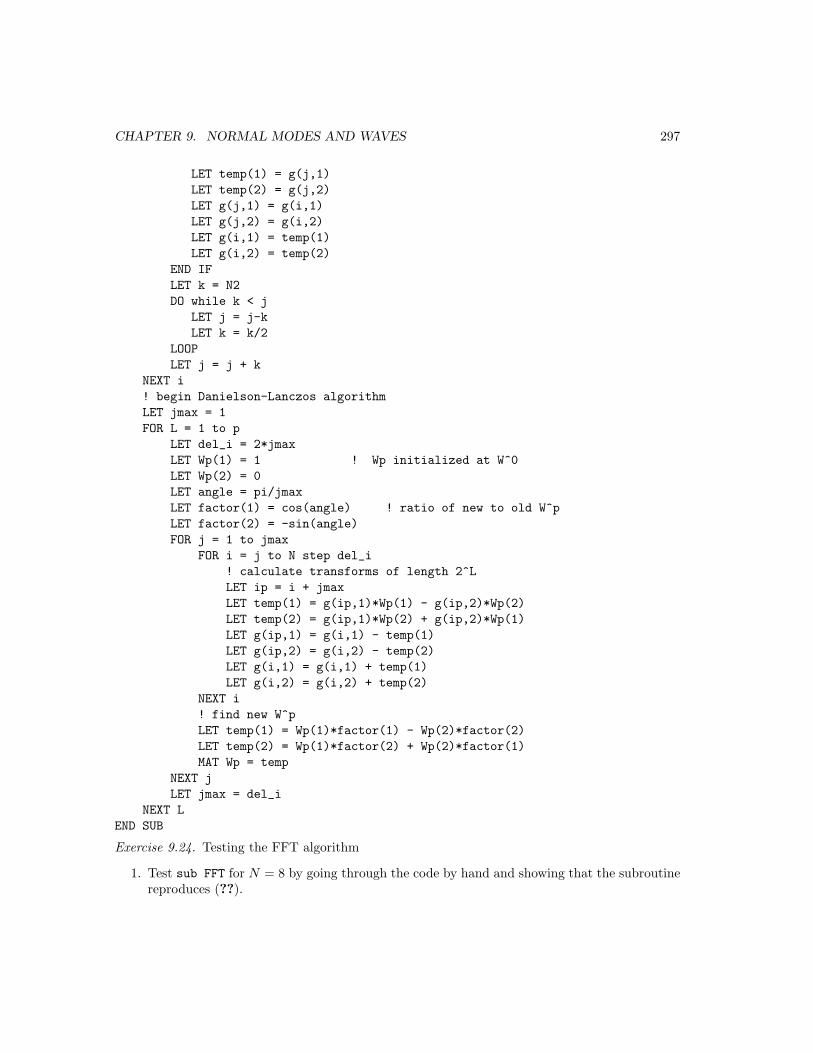
CHAPTER 9. NORMAL MODES AND WAVES 297
LET temp(1) = g(j,1)LET temp(2) = g(j,2)LET g(j,1) = g(i,1)LET g(j,2) = g(i,2)LET g(i,1) = temp(1)LET g(i,2) = temp(2)
END IFLET k = N2DO while k < j
LET j = j-kLET k = k/2
LOOPLET j = j + k
NEXT i! begin Danielson-Lanczos algorithmLET jmax = 1FOR L = 1 to p
LET del_i = 2*jmaxLET Wp(1) = 1 ! Wp initialized at W^0LET Wp(2) = 0LET angle = pi/jmaxLET factor(1) = cos(angle) ! ratio of new to old W^pLET factor(2) = -sin(angle)FOR j = 1 to jmax
FOR i = j to N step del_i! calculate transforms of length 2^LLET ip = i + jmaxLET temp(1) = g(ip,1)*Wp(1) - g(ip,2)*Wp(2)LET temp(2) = g(ip,1)*Wp(2) + g(ip,2)*Wp(1)LET g(ip,1) = g(i,1) - temp(1)LET g(ip,2) = g(i,2) - temp(2)LET g(i,1) = g(i,1) + temp(1)LET g(i,2) = g(i,2) + temp(2)
NEXT i! find new W^pLET temp(1) = Wp(1)*factor(1) - Wp(2)*factor(2)LET temp(2) = Wp(1)*factor(2) + Wp(2)*factor(1)MAT Wp = temp
NEXT jLET jmax = del_i
NEXT LEND SUB
Exercise 9.24. Testing the FFT algorithm
1. Test sub FFT for N = 8 by going through the code by hand and showing that the subroutinereproduces (??).

CHAPTER 9. NORMAL MODES AND WAVES 298
2. Write a subroutine to do the Fourier transform in the conventional manner based on (??).Make sure that your subroutine has the same arguments as SUB FFT, that is, write a sub-routine to convert f(j∆) to the two-dimensional array g. If the data is real, let g(i,2) = 0.The subroutine should consist of two nested loops, one over k and one over j. Print theFourier transform of random real values of f(j∆) for N = 8, using both SUB FFT and thedirect computation of the Fourier transform. Compare the two sets of data to insure thatthere are no errors in SUB FFT. Repeat for a random collection of complex data points.
3. Compute the CPU time as a function of N for N = 16, 64, 256, and 1024 for the FFTalgorithm and the direct computation. You can use the time function in True BASIC beforeand after each call to the subroutines. Verify that the dependence on N is what you expect.
4. Modify SUB FFT to compute the inverse Fourier transform defined by (??). The inverseFourier transform of a Fourier transformed data set should be the original data set.
References and Suggestions for Further Reading
E. Oran Brigham, The Fast Fourier Transform, Prentice Hall (1988). A classic text on Fouriertransform methods.
David C. Champeney, Fourier Transforms and Their Physical Applications, Academic Press(1973).
James B. Cole, Rudolph A. Krutar, Susan K. Numrich, and Dennis B. Creamer, “Finite-differencetime-domain simulations of wave propagation and scattering as a research and educationaltool,” Computers in Physics 9, 235 (1995).
Frank S. Crawford, Waves, Berkeley Physics Course, Vol. 3, McGraw-Hill (1968). A delightfulbook on waves of all types. The home experiments are highly recommended. One observationof wave phenomena equals many computer demonstrations.
Paul DeVries, A First Course in Computational Physics, John Wiley & Sons (1994). Part of ourdiscussion of the wave equation is based on Chapter 7. There also are good sections on thenumerical solution of other partial differential equations, Fourier transforms, and the FFT.
N. A. Dodd, “Computer simulation of diffraction patterns,” Phys. Educ. 18, 294 (1983).
P. G. Drazin and R. S. Johnson, Solitons: an Introduction, Cambridge (1989). This book focuseson analytical solutions to the Korteweg-de Vries equation which has soliton solutions.
Richard P. Feynman, Robert B. Leighton, and Matthew Sands, The Feynman Lectures on Physics,Vol. 1, Addison-Wesley (1963). Chapters relevant to wave phenomena include Chapters 28–30and Chapter 33.
A. P. French, Vibrations and Waves, W. W. Norton & Co. (1971). An introductory level text thatemphasizes mechanical systems.
CHAPTER 9. NORMAL MODES AND WAVES 299
Eugene Hecht, Optics, second edition, Addison-Wesley & Sons (1987). An intermediate level opticstext that emphasizes wave concepts.
Akira Hirose and Karl E. Lonngren, Introduction to Wave Phenomena, John Wiley & Sons (1985).An intermediate level text that treats the general properties of waves in various contexts.
Amy Kolan, Barry Cipra, and Bill Titus, “Exploring localization in nonperiodic systems,” Com-puters in Physics 9, to be published (1995). An elementary discussion of how to solve theproblem of a chain of coupled oscillators with disorder using transfer matrices.
William H. Press, Saul A. Teukolsky, William T. Vetterling, and Brian P. Flannery, NumericalRecipes, second edition, Cambridge University Press (1992). See Chapter 12 for a discussionof the fast Fourier transform.
Timothy J. Rolfe, Stuart A. Rice, and John Dancz, “A numerical study of large amplitude motionon a chain of coupled nonlinear oscillators,” J. Chem. Phys. 70, 26 (1979). Problem ?? isbased on this paper.
Garrison Sposito, An Introduction to Classical Dynamics, John Wiley & Sons (1976). A gooddiscussion of the coupled harmonic oscillator problem is given in Chapter 6.
William J. Thompson, Computing for Scientists and Engineers, John Wiley & Sons (1992). SeeChapters 9 and 10 for a discussion of Fourier transform methods.
Michael L. Williams and Humphrey J. Maris, “Numerical study of phonon localization in dis-ordered systems,” Phys. Rev. B 31, 4508 (1985). The authors consider the normal modesof a two-dimensional system of coupled oscillators with random masses. The idea of usingmechanical resonance to extract the normal modes is the basis of a new numerical method forfinding the eigenmodes of large lattices. See Kousuke Yukubo, Tsuneyoshi Nakayama, andHumphrey J. Maris, “Analysis of a new method for finding eigenmodes of very large latticesystems,” J. Phys. Soc. Japan 60, 3249 (1991).