wavelet - pair copula construction inference for financial ... · wavelet - pair copula...

Wavelet - Pair Copula Construction Inference for Financial Contagion

MARCELO BRUTTI RIGHI¹, PAULO SERGIO CERETTA² Departament of Business

Federal Universityof Santa Maria Avenue Roraima, 1000, Rio Grande do Sul

BRAZIL [email protected]¹, [email protected]²

Abstract - In this paper we propose a Wavelet - Pair Copula Construction approach for contagion identification. The method consists in filtering past marginal dependence, performing multiscale decomposition in marginal residuals, and estimating a Pair Copula Construction for each frequency scale of interest. We carry out these steps with daily data from U.S., German, Brazilian and Hong Kong MSCI indices. The procedure is realized for non-crisis and crisis (sub-prime and Eurozone) periods. We find results that indicate a rising in association for most relationships, representing presence of contagion effect during Sub-prime and Eurozone crises. Key-Words: Risk Analysis, Contagion, Wavelets, Pair Copula Construction, financial markets, dependence. 1Introduction

The global extent of recent crises and potential damaging consequences of contagion continuously attract attention among economists and policymakers. The transmission of shocks to other countries and cross-countries correlations, beyond any fundamental link, have long been an issue of interest to academics, fund managers and traders, as it have important implications for portfolio allocation and asset pricing [1].

[2] define contagion as a significant increase in cross-market linkages after a shock to one country (or group of countries), otherwise, a continued market correlation at high levels is considered to be no contagion, only interdependence. Since then, the existence of financial contagion has been studied by many researchers, mainly around the notion of correlation breakdown, i.e., a statistically significant increase in correlation during crash period. Such pattern suggests that benefits of international diversification for asset allocation and portfolio composition may be substantially reduced in stressful market situations, just when these benefits are most needed.

Despite the large number of papers about financial market contagion, there is no agreement in literature on exact definition of what constitutes contagion and how we should measure it. The major distinction when defining contagion is between ‘‘fundamentals-based’’ and ‘‘pure’’ contagion. [3] define ‘‘fundamentals-based’’ contagion as the transmission of shocks between markets resulting from financial market integration in both crisis and

non-crisis periods (spillovers). In other hand, [4] define ‘‘pure’’ contagion as shocks transmission from one market to another market after controlling fundamental factors.

Regarding to measurement, a first approach is to test correlation changes, as performed by [5,3, 6,7]. Econometric time series models predominate as statistical technique for contagion inferece. The use of univariate and multivariate GARCH models is well documented in the works of [8, 9, 10, 11, 12, 13]. Long term cointegrating relationships are reported in studies of [14, 15, 16, 17]. Logit/Probit classification models appear in [4, 18, 19]. Linear or regime-switching VAR models are used by [20,21, 22, 23] . The extreme value theory is addressed for contagion in [24, 25].

Despite this classical time series model approaches, it has emerged the use of more sophisticated tools for contagion identification. One technique is the copula approach for dependence. Recent studies have ascertained the superiority of copulas to model dependence, because a copula function can deal with non-linearity, asymmetry, serial dependence and also the well-known heavy-tails of financial assets marginal and joint probability distribution. Recently, some works employed copula methods for contagion, as [26, 27, 28, 29]. Other potentially useful technique is the wavelet approach for frequency domain analysis. Given its ability to partition each variable into components of different frequencies, it can provide a simple and intuitive way to distinguish between contagion and interdependence. Studies with this tool for contagion identification were realized by

WSEAS TRANSACTIONS on BUSINESS and ECONOMICS Marcelo Brutti Righi, Paulo Sergio Ceretta

E-ISSN: 2224-2899 648 Volume 11, 2014

[30, 31,32].Based on this methodological evolution, we aim to use a contagion identification approach which links the advantages of wavelet and copula features. To that we decompose time series in multiscales with wavelet analysis and we estimate dependence in these distinct frequencies through copula functions. For this purpose we use Pair Copula Construction (PCC), which can more effectively lead with structures composed by more than two variables. Once contagion is a multivariate issue, this property can be very useful. PCC is based on a decomposition of a multivariate density into bivariate copula densities, of which some are dependency structures of unconditional bivariate distributions, and the rest are dependency structures of conditional bivariate distributions.

Thus, the paper main contribution for literature is wavelet multiscale decomposition and PCC dependence structure association for contagion effect identification. We compare the association of the U.S., German, Brazilian and Hong Kong stock markets considering periods referring to crisis (sub-prime and Eurozone) and non-crisis (before sub-prime).

The remainder of this paper is structured as follows: section 2 presents the methodological procedures of proposed wavelet-PCC based contagion inference, jointly with a brief background about wavelets, copula functions and PCC methods. Section 3 exposes an empirical illustration; Section 4 concludes the paper.

2 Theory Suppose that financial returns follow some

marginal time series models which takes into account the conditional behavior of financial assets means ( ) and variances ( ). Once assets have their past marginal dependence filtered by these models, we can analyze joint relationship. To that, we use the estimated residual from marginal models. We perform multiscale decomposition in these residuals series through wavelets.

Wavelets, as is suggested by their name, are little waves. The term wavelet was created in the geophysics literature by [33]. However, the evolution of wavelets occurred over a significant time scale and in manydisciplines, and their background can be found in [34,35, 36, 37, 38], among others.

Basic wavelets are characterized into father and mother wavelets. A father wavelet (scaling function) represents the smooth baseline trend, while mother wavelets (wavelet function) are used to describe all

deviations from trends. Father and Mother Wavelets are represented by formulations (1) and (2), respectively.

. (1)

. (2) Where , for some coarse scale , that

will be taken as zero. From these expressions an orthonormal system is generated. For any function f that belongs to this system we may write, uniquely:

. (3)

In (3), and are the wavelet coefficients. Thus,

consider a time series, f (t), which we want to decompose into various wavelet scales. Given the father wavelet, such that its dilates and translates constitute orthonormal bases for all the subspaces that are scaled versions of the initial subspace, we can form a Multiresolution Analysis (MRA) for f(t).The wavelet function in (3) depends on two parameters, scale and time: the scale or dilation factor j controls the length of the wavelet, while the translation or location parameter k refers to the location and indicates the non-zero portion of each wavelet basis vector.

Thus, each series is decomposed into two parts: a low-frequency part, which can be associated to interdependence, and a high frequency part, which is what remains after interdependence is taken into account, that is contagion [32]. Specifically, the wavelet coefficients can be straightforwardly manipulated to obtain recognizable statistical quantities such as wavelet variance, wavelet covariance, and wavelet correlation [39, 40]. We extend this linear statement to a non-linear approach. Thus, the fundamental idea is, for each frequency level of interest, we estimate a PCC with decomposed marginal residuals in order to obtain dependence measures for each bivariate relationship. This procedure is done for non-crisis and crisis periods. If one notes a rising in these levels associations, a contagion effect is noticed.

In order to best explain the PCC concept, we begin by briefly presenting copula methods. A copula returns joint probability of events as a function of each event marginal probabilities. This property makes copulas attractive, as the univariate marginal behavior of random variables can be modeled separately from their dependence.

The concept of copula was introduced by [41]. However, only recently its applications have become clear. A detailed treatment of copulas as


E-ISSN: 2224-2899 649 Volume 11, 2014

well their relationship to concepts of dependence is given by [42, 43]. A review of applications of copulas to finance can be found in [44, 45].

A function is a copula if, for and

it fulfills the following properties:

(4)

(5) Property (4) means uniformity of the margins,

while (5), the n-increasing property means that for (X,Y)

with distribution function C. In the seminal paper of [41], it was

demonstrated that a Copula is linked with a distribution function and its marginal distributions. This important theorem states that:

(i) Let C be a copula and and univariate distribution functions. Then (6) defines a distribution function F with marginal and .

(6) (ii) For a two-dimensional distribution function F

with marginal and , there exists a copula C satisfying (6). This is unique if and are continuous and then, for every :

(7) In (7), denote the generalized left

continuous inverses of and . Regarding to the estimation, the dominant methods are traditional maximum likelihood (ML), pseudo-maximum likelihood (PML), proposed by [46], and inversion of dependence measures like Spearman’s Rho and Kendall’s Tau. [47] developed an extension of the pseudo-maximum likelihood to markovian time series.

However, it is not always obvious to identify the copula. Indeed, accordingly [48], for many financial applications, the problem is not to use a given multivariate distribution but consists in finding a convenient distribution to describe some stylized facts, for example the relationships between different asset returns. [49] present a great overview of the goodness of fit and selection issues of copula families.

Since copulas are linked to the dependence structure, they must be related to dependence measures. We present here calculation procedures, adapted from [50], of the most representative dependence measures for financial purposes. We keep same notation. Given the estimated bivariate copula C, lower and upper tail dependence, are

represented by formulations (8) and (9), respectively. Absolute dependence calculated with Kendall’s Tau through the conversion of bivariate copulas is exposed in formulation (10).

. (8)

. (9)

(10) Such copulas can be used in order to construct a

more complex dependence structure, the PCC. PCC is a very flexible construction, which allows for free specification of n(n−1)/2 bivariate copulas. This construction was proposed by [51], and it has been discussed in detail, especially, for applications in simulation and inference [52, 53, 54].The PCC is hierarchical in nature. The modeling scheme is based on a decomposition of a multivariate density into n(n−1)/2 bivariate copula densities, of which the first n−1 are dependency structures of unconditional bivariate distributions, and the rest are dependency structures of conditional bivariate distributions [55].

The PCC is usually represented in terms of the density. The two main types of PCC that have been proposed in literature are the C (canonical)-vines and D-vines. In the present paper we focus on the D-vine estimation, which accordingly to [56] has density as in formulation (11).

(11) In (11), are variables; is the density

function; is a bivariate copula density. Conditional distribution functions are computed, accordingly to Joe (1996), by formulation (12).

. (12)

In (12) is the bivariate conditional distribution dependence structure of x and

conditioned on , where the vector is the vector v excluding the component . To become possible to use the D-vine construction to represent a dependence structure through copulas, we must assume that univariate margins are uniform in interval [0,1]. Therefore, the conditional distributions involved at one level of construction are always computed as partial derivatives of bivariate copulas at previous level [55]. Since only bivariate copulas are involved, partial derivatives may be obtained relatively easy for most parametric copula families. It is worth to note that the copulas


E-ISSN: 2224-2899 650 Volume 11, 2014

involved in (11) do not need to belong to same family. We should choose, for each pair of variables, the parametric copula that best fits the data.

Concerning to the estimation of PCC parameters, [56] propose a ML estimation procedure which follows a stepwise approach. In a first step one compute ML estimates of the parameters of each pair-copula family separately. The parameter estimates obtained in this first step are known as sequential ML estimates. In a second step the full log-likelihood function is maximized jointly using the sequential ML estimates as starting values, resulting in the so-called joint ML estimates. Regarding to empirical literature, studies point out for superiority of PCC over other copula structures in finance [55, 57, 58, 59].

3 Results and discussion For a detailed empirical illustration, we use daily

data from MSCI indices from U.S., German, Brazilian and Hong Kong stock markets from June 2005, to June 2012, totalizing 1744 observations. The first two markets are developed countries which were initially affected by the two crises present in sample period (sub-prime and Eurozone). The last two markets are emerging ones and are potential contagion sufferers, once they are used for international diversification. We prefer to use just one market of each continent in order to avoid too much dependence due to geographic factors. These indices were chosen because they represent the stock market activity in these countries and can avoid possible non-synchronous biases caused by the usual market indices.

For crisis and non-crisis sample periods division, we proceed as follows: For sub-prime crisis period we consider 512 trading days starting in August, 2007, which is the real state bubble “burst”. The 512 trading days before this date were considered non-crisis period. For the Eurozone debt crisis we consider 512 trading days starting in July 2010, as pointed by [60], based on structural change tests. The use of this length (512 trading days) is based on fact that wavelet analysis is performed considering data lengths with power of 2 (512=29). Despite some techniques, as maximal overlap discrete wavelet transform (MODWT), can handle any sample size we chose the traditional approach to avoid any possible bias occasioned by distinct sample sizes in crisis and non-crisis periods.

Fig. 1 and 2 present, respectively, plots of the studied indices daily prices and log-returns, indicating the three time windows previously cited.

The non-crisis period (from beginning to first vertical line) correspond to a rising trend in market prices and low volatile market log-returns. In the sub-prime period (between first and second vertical lines) there is a falling trend in market prices and huge log-returns volatility clusters. The Eurozone crisis (between third and fourth vertical lines) presented an initial fall in prices and volatile returns. After a relative recovering and calm period there were larger price falls and volatility clusters. Fig. 1 and 2 plots elucidate distinct occurred behaviors during whole sample period.

In order to numerical illustrate this distinction we present in Table 1 some descriptive statistics considering the periods division. Results in Table 1 indicate that sub-prime crisis was the most turbulent period, followed by Eurozone crisis and non-crisis period. This result is elucidated by range values (maximum – minimum), as well as standard deviations. In all time divisions emerging markets exhibited more risk than developed ones. This fact is linked with distinct economic maturity and liquidity level, which are higher in developed markets. The central tendency measures were always very close to zero. There is predominance of the well-known negative asymmetric leptokurtic behavior [25]. Moreover, this leptokurtosis was more intense during crisis periods, reflecting the presence of extreme returns.

Descriptive results in Table 1 allied with Fig. 1 and 2 graphical analyses clearly indicate vestiges of changes on studied markets marginal behavior in crisis and non-crisis periods. Nonetheless, we are fundamentally interested in markets joint behavior. The first step is to filter marginal past dependence. To that we need to consider the conditional heteroscedastic pattern of financial time series, just like the identified asymmetric leptokurtic behavior of these log-returns.

Thus, we estimate ARMA (m,n) - GARCH (p,q) models with skewed student’s t innovations. The estimated model is represented in formulation (13).

, ,

(13) Where is the log-return of asset i in period t; is the conditional variance of asset i in period t;

, , , , and are parameters; is the innovation on conditional mean of asset i in period t; represents a skewed student’s t with v degrees of freedom white noise. The choices for this ARMA-GARCH model over others (ARFIMA, APARCH, GJR-GARCH, etc.), lags number to


E-ISSN: 2224-2899 651 Volume 11, 2014

include in mean and variance equations, as well innovations distribution is based on correlogram and AIC criterion. Estimated models are validated by the verification of serial correlation in linear and squared standardized residuals through Q statistic. For parsimony questions we do not present the results for this marginal estimation once these marginal issues are not the paper scope.

With filtered residuals we are able to investigate joint patterns with no marginal influence. We standardize the marginal residuals into pseudo-observations through the ranks as ). With these standardized residuals we perform a time-scale decomposition analysis for non-crisis and crisis periods through wavelets, as explained in section 2. Previous studies ([61], for example) on high-frequency data have shown that a moderate-length filter such as L = 8 is adequate. Hence, we use the Daubechies compactly supported least asymmetric wavelet filter of length L = 8, based on eight non-zero coefficients with reflecting boundary conditions [34]. We also used Daubechies extremal phase wavelet filter of distinct lengths for comparison, but we obtained similar results. The same choice was performed, for instance, in [32].

Several papers suggest that transmission of shocks due to contagion in international financial markets is very fast and dies out quickly after a one or two weeks at most (see, for example, [62]).As contagion effects generally do not exceed one or two weeks, we can assume that the last four wavelet levels provide a realistic measure of contagion, as these very fine scales are associated to changes of 1, 2, 4, and 8 days, respectively. Recalling that our data sets are composed by 512=29 observations, we get 9 scales. Therefore, ‘‘pure’’ contagion is measured by 6, 7, 8 and 9 levels wavelet coefficients, i.e., coefficients corresponding to (finest) scales up to 2 weeks, and ‘‘fundamental-based’’ contagion by (coarse) levels 1 to 5.

For the dependence estimation, we use PCC, conform presented in section 2, in levels 6 to 9, in crisis and non-crisis periods. The parameters are estimated through maximum likelihood as proposed by [56]. To choose the copula that best fits each bivariate pair of variables we employ AIC criterion. The candidate families were Normal, Student’s t, Clayton, Gumbel, Frank, Joe, BB1, BB6, BB7 and BB8. Definitions about these copula families can be found in [42]. In order to test the estimated parameter significance, we perform some t ratio tests like with n – k degrees of freedom. This is possible because, as pointed out by

[42], the ML estimation for copulas is asymptotically normallly distributed.

After, we calculate Kendall’s Tau through the estimated PCC parameters, conform (10). We chose to use Kendall’s Tau in this illustration because it is an absolute measure (just like traditional correlation), i.e., it is not restricted to some distribution quantile or interval. Tables 2, 3 and 4 present PCC estimation results for non-crisis, sub-prime crisis and Eurozone crisis periods, respectively.

Results in Tables 2 to 4 indicate the presence of many copula families in bivariate relationships such that there is no predominance of any family. In this sense, bivariate relationships that presented the same family to all analyzed scales are rare. All estimated parameters obtained statistical significance, indicating proper fit. Most relationships exhibited changes in Kendall’s Tau through distinct levels. It is valid to highlight that PCC isolates interference from variables not included in each bivariate relation, exhibiting a trend for decreasing behavior in the direction of the initial levels of the vine to the final ones. Some pairs exhibited negative association, as is USA/Hong Kong case. Regarding to periods distinction, one can note a general rising trend in Tau values in both crisis periods in comparison with non-crisis period. Fig. 3 presents a graphical complement to this question.

Fig. 3 patterns visually elucidate that there is vestige for a rise in association for most cases, indicating presence of contagion effect during Sub-prime and Eurozone crises. This result is reinforced by PCC nature, which isolates influence from other markets in each bivariate relationship. In general, sub-prime crisis period obtained higher Tau values in pairs than Eurozone crisis period, except for USA/Germany relation. Moreover, it is fundamental realize that these contagion effects are wavelet level dependent, in the sense that they do not display their effects uniformly across scales. Particularly, the relations of Hong Kong with Germany at level 7, and USA at level 8 exhibited relevant association change during sub-prime period, once not just changed dependence magnitude, as well wavelet level pattern. In sum, obtained results indicate that Wavelet-PCC approach is an efficient tool for contagion inference, because combines advantages of two sophisticated and robust techniques.

4 Conclusion

In this paper we proposed a Wavelet-PCC contagion identification approach. The method consists in three steps: i) To filter marginal past


E-ISSN: 2224-2899 652 Volume 11, 2014

dependence with some univariate financial time-series model; ii) To perform multiscale decomposition in marginal models residuals series through wavelets, decomposing these residuals series into two parts: a low-frequency part, which can be associated to interdependence, and a high frequency part, which is contagion; iii) For each frequency scale of interest, to estimate a PCC in order to obtain dependence measures for each bivariate relationship.

We performed these steps with daily data from U.S., German, Brazilian and Hong Kong MSCI indices. The procedure was realized for non-crisis and crisis (sub-prime and Eurozone) periods. We found results that indicate rising in association for most relationships, representing presence of

contagion effect during Sub-prime and Eurozone crises. In general, sub-prime crisis period obtained higher Tau values than Eurozone crisis period. Moreover, contagion effects were wavelet level dependent, in the sense that they do not display their effects uniformly across scales. Thus, the proposed Wavelet-PCC approach can be considered a tool for contagion inference, especially because it combines advantages of these two sophisticated and robust techniques. We suggest for future research that one applies the proposed approach for other assets and markets, as well as distinct frequencies and temporal samples, to give diffusion and robustness to this method.

References: [1] Kenourgios, D., Samitas, A., Paltalidis, N.,

Financial crises and stock market contagion in a multivariate time-varying asymmetric framework, Journal of International Financial Markets, Institutions and Money, Vol. 21, 2011, pp. 92-106.

[2] Forbes, K.J., & Rigobon, R., No contagion, only interdependence: measuring stock market comovements, The Journal of Finance, Vol. 57, 2002, pp. 2223–2261.

[3] Reinhart, C., Calvo, S., Capital flows to Latin America: is there evidence of contagion effects? In: G. Calvo, M. Goldstein, E. Hochreiter (Eds.), Private Capital Flows to Emerging Markets After the Mexican Crisis. Washington: Institute for International Economics, 1996.

[4] Bae, K.-H., Karolyi, G. A., Stulz, R., A new approach to measuring financial contagion, Review of Financial Studies, Vol. 16, 2003, pp. 716–763.

[5] King, M., Wadhwani, S., Transmission of volatility between stock markets, Review of Financial Studies, Vol. 3, 1990, pp. 5–33.

[6] Baig, T., Goldfajn, I., Financial market contagion in the Asian crisis, IMF Staff Papers, Vol. 46, No. 2, 1999, pp. 167-195.

[7] Hon, M.T., Strauss, J.K., Yong, S.-K., Deconstructing the Nasdaq bubble: a look at contagion across international stock markets, Journal of International Financial Markets, Institutions and Money, Vol. 17, 2007, pp. 213–230.

[8] Hamao, Y., Masulis, R.W., Ng, V., Correlations in price changes and volatility

across international stock markets, Review of Financial Studies, Vol. 3, 1990, pp. 281–307.

[9] Chou, R.Y.-T., Ng, V., Pi, L.K., Cointegration of international stock market indices, IMF Working Papers, 1994.

[10] Edwards, S., Interest rate volatility, capital controls, and contagion. NBER Working Paper, No. 6756, 1998.

[11] Bekaert, G., Wu, G., Asymmetric volatility and risk in equity markets, Review of Financial Studies, Vol. 13, 2000, pp. 1–42.

[12] Chiang, T.C., Jeon, B.N., Li, H., Dynamic correlation analysis of financial contagion: evidence from Asian markets, Journal of International Money and Finance, Vol. 26, 2007, pp. 1206–1228.

[13] Billio, M., Caporin, M., Market linkages, variance spillovers, and correlation stability: empirical evidence of financial contagion, Computational Statistics & Data Analysis, Vol. 54, 2010, pp. 2443–2458.

[14] Longin, F., Is the correlation in international equity returns constant: 1960–1990? Journal of International Money and Finance, Vol. 14, 1995, pp. 3–26.

[15] Cashin, P., Kumar, M.S., McDermott, C.J., International integration of equity markets and contagion effects, IMF Working Papers, No. 110, 1995.

[16] Östermark, R., Multivariate cointegration analysis of the Finnish–Japanese stock markets, European Journal of Operational Research, Vol.134, 2001, pp. 498–507.

[17] Bekaert, G., Harvey, C. R., Ng, A., Market integration and contagion, Journal of Business, Vol. 78, 2005, pp. 39–69.

[18] Eichengreen, B., Rose, A.K., Wyplosz, C., Contagious currency crises: first tests,


E-ISSN: 2224-2899 653 Volume 11, 2014

TheScandinavian Journal of Statistics, Vol. 98, 1996, pp. 463–484.

[19] Kaminsky, G. L., Reinhart, C. M., On crises, contagion, and confusion, Journal of International Economics, Vol. 51, 2000, pp. 145–168.

[20] Favero, C.A., Giavazzi, F., 2002. Is the international propagation of financial shocks non-linear? Evidence from the ERM. Journal of International Economics, 57, 231–246.

[21] Yang, J., & Bessler, D.A., Contagion around the October 1987 stock market crash, European Journal of Operational Research, Vol. 184, 2008, pp. 291–310.

[22] Gallo, G.M., Otranto, E., Volatility spillovers, interdependence and comovements: a Markov switching approach, Computational Statistics & Data Analysis, Vol. 52, 2008, pp. 3011–3026.

[23] Guo, F., Chen, C. R., Huang, Y. S., Markets contagion during financial crisis: A regime-switching approach, International Review of Economics and Finance, Vol. 20, 2011, pp. 95–109.

[24] Quintos, C., Fan, Z., Philips, P.C.B., Structural change tests in tail behaviour and the Asian crisis, The Review of Economics Studies, Vol. 68, 2001, pp. 633–663.

[25] Longin, F., Solnik, B., Extreme Correlation of International Equity Markets, Journal of Finance, Vol. 56, 2001, pp. 649–676.

[26] Rodriguez, J.C., Measuring financial contagion: a copula approach, Journal of Empirical Finance, Vol. 14, 2007, pp. 401–423.

[27] Okimoto, T., New evidence of asymmetric dependence structures in international equity markets, Journal of Financial and Quantitative Analysis, Vol. 43, 2008, pp. 787–815.

[28] Jayech, S., Zina, N.B., A copula-based approach to financial contagion in the foreign exchange markets, International Journal of Mathematical Operational Research, Vol. 3, 2011, pp. 636–657.

[29] Aloui, R., Aïssa., M. S. B., Nguyen, D. K., Global financial crisis, extreme interdependences, and contagion effects: The role of economic structure? Journal of Banking & Finance, Vol. 35, 2011, pp. 130–141.

[30] Bodart, V., Candelon, B., Evidence of interdependence and contagion using a frequency domain framework, Emerging Markets Review, Vol. 10, 2009, pp. 140–150.

[31] Orlov, A., Cospectral analysis of exchange rate comovements during Asian financial crisis, Journal of International Financial Markets,

Institutions and Money, Vol. 19, 2009, pp. 742–758.

[32] Gallegati, M., A wavelet-based approach to test for financial market contagion, Computational Statistics & Data Analysis, Vol. 56, 2012, pp. 3491–3497.

[33] Morlet, J., Arens, G., Fourgeau, E., Glard, D., Wave propagation and sampling theory—Part I: complex signal and scattering in multilayered media. Geophysics, Vol. 47, 1982, pp. 203–221.

[34] Daubechies, I., Ten Lectures on Wavelets. CBSM-NSF Regional Conference Series in Applied Mathematics, Philadelphia, 1992.

[35] Meyer, Y., Wavelets: Algorithms and Applications, SIAM, Philadelphia, 1993.

[36] Vidakovic, B.,Statistical Modeling by Wavelets, Wiley Series in Probability and Statistics, 1999.

[37] Gençay, R., Selçuk, F., Whitcher, B., Systematic risk and timescales, Quantitative Finance, Vol. 3, 2003, pp. 108–116.

[38] Heil, C., Walnut, D.F., Fundamental Papers in Wavelet Theory, New Jersey: Princeton University Press, 2006.

[39] Percival, D.B., On estimation of the wavelet variance, Biometrika, Vol. 82, 1995, pp. 619–631.

[40] Whitcher, B., Guttorp, P., Percival, D.B., Wavelet analysis of covariance with application to atmospheric time series, Journal of Geophysical Research Atmospheres, Vol. 105, 2000, pp. 14941–14962.

[41] Sklar, A., Fonctions de Repartition á n Dimensions et leurs Marges, Publications de l'Institut de Statistique de l'Université de Paris, Vol. 8, 1959, pp. 229-231.

[42] Joe, H., Multivariate models and dependence concepts, Chapman Hall, 1997.

[43] Nelsen, R., An introduction to copulas, New York: Springer, 2006.

[44] Embrechts P., Lindskog F., McNeil A., Modeling dependence with copulas and applications to Risk Management. In: Handbook of Heavy Tailed Distributions in Finance, ed. S. Rachev, Elsevier, Chapter 8, 2003, pp. 329-384.

[45] Cherubini, U., Luciano, E., Vecchiato, W., Copula Methods in Finance, Chichester: Wiley, 2004.

[46] Genest, C., Ghoudi, K., Rivest, L.-P., A semiparametric estimation procedure of dependence parameters in multivariate families of distributions, Biometrika, Vol. 82, 1995, pp. 543–552.


E-ISSN: 2224-2899 654 Volume 11, 2014

[47] Chen, X., Fan, Y., Estimation and model selection of semiparametric copula-based multivariate dynamic models under copula misspecification, Journal of Econometrics, Vol. 135, 2006, pp. 125 – 154.

[48] Berrada, T., Dupuis, D. J., Jacquier, E., Papageorgiou, N., Rémillard, B., Credit migration and derivatives pricing using copulas, Journal of Computational Finance, Vol. 10, 2006, pp. 43–68.

[49] Genest, C., Rémillard, B., & Beaudoin, D., Omnibus goodness-of-fit tests for copulas: A review and a power study, Insurance: Mathematics and Economics, Vol. 44, 2009, pp. 199–213.

[50] Cherubini, U., Mulinacci, S., Gobbi, F., Romagnoli, S., Dynamic Copula Methods in Finance, John Wiley & Sons, 2012.

[51] Joe, H., Families of m-variate distributions with given margins and m(m-1)/2 bivariate dependence parameters. Distributions with Fixed Marginals and Related Topics. Institute of Mathematical Statistics, California, 1996.

[52] Bedford, T., Cooke, R., Probability density decomposition for conditionally dependent random variables modeled by vines, Annals of Mathematical Artificial Intelligence, Vol. 32, 2001, pp. 245–268.

[53] Bedford, T., Cooke, R. M., Vines: A new graphical model for dependent random variables, The Annals of Statistics, Vol. 30, 2002, pp. 1031–1068.

[54] Kurowicka, D., Cooke, R.M., Uncertainty Analysis with High Dimensional Dependence Modelling, New York: Wiley, 2006.

[55] Aas, K., Berg, D., Modeling Dependence Between Financial Returns Using PCC. In: D. Kurowicka, & H. Joe (Eds.). Dependence Modeling: Vine Copula Handbook, World Scientific,2011, pp.305-328.

[56] Aas, K., Czado, C., Frigessi, A., Bakken, H., Pair-copula constructions of multiple dependence, Insurance: Mathematics and Economics, Vol. 44, No. 2, 2009, pp. 182–198.

[57] Chollete, L., Heinen, A., Valdesogo, A., Modeling international financial returns with a multivariate regime-switching copula, Journal of Financial Econometrics, Vol. 7, 2009, pp. 437–480.

[58] Fischer, M., Köck, C., Schlüter, S., Weigert, F., An empirical analysis of multivariate copula models, Quantitative Finance, Vol. 9, 2009, pp. 839–854.

[59] Czado, C., Schepsmeier, U., Min, A., Maximum likelihood estimation of mixed C-vines with application to exchange rates, Statistical Modeling, Vol. 12, 2012, pp. 229-255.

[60] Righi, M.B., Ceretta, P.S., Analyzing the structural behavior of volatility in the Major European Markets during the Greek crisis, Economics Bulletin, Vol. 31, 2011, pp. 3016-3029.

[61] Gençay, R., Selçuk, F., Whitcher, B., Multiscale systematic risk, Journal of International Money and Finance, Vol. 24, 2005, pp. 55–70.

[62] Ait-Sahalia, J., Cacho-Diaz, J., Laeven, R., Modeling financial contagion using mutually exciting jump processes, NBER Working Paper, 15850, 2010.


E-ISSN: 2224-2899 655 Volume 11, 2014

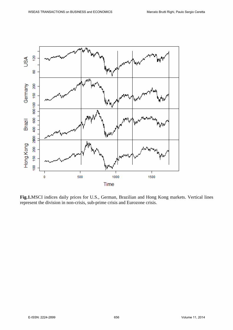
Fig.1.MSCI indices daily prices for U.S., German, Brazilian and Hong Kong markets. Vertical lines represent the division in non-crisis, sub-prime crisis and Eurozone crisis.


E-ISSN: 2224-2899 656 Volume 11, 2014

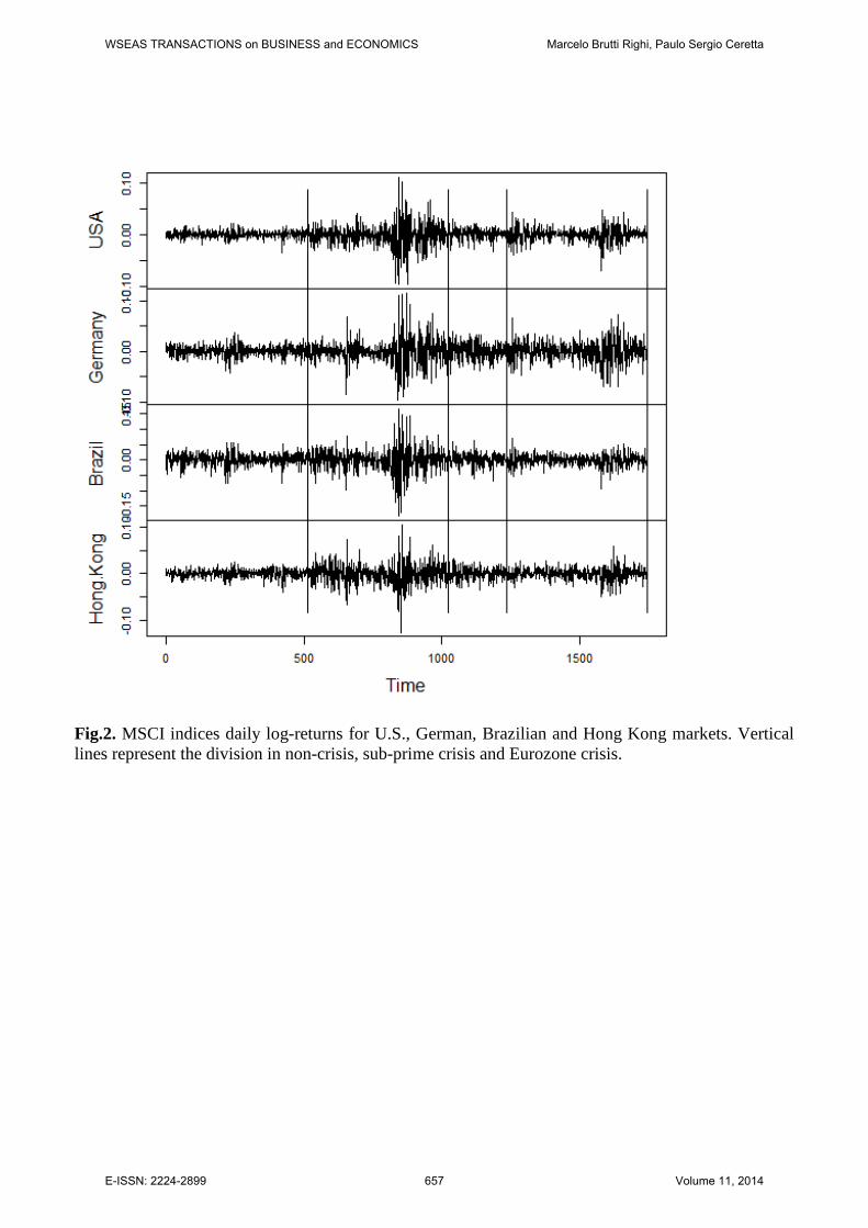
Fig.2. MSCI indices daily log-returns for U.S., German, Brazilian and Hong Kong markets. Vertical lines represent the division in non-crisis, sub-prime crisis and Eurozone crisis.


E-ISSN: 2224-2899 657 Volume 11, 2014

Fig.3.Kendall’s Tau association measure of the U.S., German, Brazilian and Hong Kong MSCI indices daily log-returns bivariate relationships through Wavelet levels 6,7,8 and 9 in non-crisis (black), sub-prime crisis (red) and Eurozone crisis (blue) periods.


E-ISSN: 2224-2899 658 Volume 11, 2014

Table 1Descriptive statistics of the MSCI indices daily log-returns for U.S., German, Brazilian and Hong Kong markets, considering non-crisis, sub-prime crisis and Eurozone crisis periods.

Statistic Minimum Maximum Mean Deviation Skewness Kurtosis Non-crisis USA -0.0350 0.0218 0.0004 0.0064 -0.3298 5.3294 Germany -0.0419 0.0378 0.0012 0.0104 -0.3009 4.0891 Brazil -0.0746 0.0581 0.0018 0.0186 -0.5761 4.6949 Hong Kong -0.0404 0.0256 0.0006 0.0083 -0.5962 4.9498 Sub-Prime USA -0.0951 0.1104 -0.0010 0.0219 -0.0737 7.2316 Germany -0.0964 0.1159 -0.0012 0.0238 0.2209 7.6899 Brazil -0.1832 0.1662 -0.0004 0.0371 -0.2339 7.1662 Hong Kong -0.1257 0.1045 -0.0005 0.0228 -0.0184 6.3177 Eurozone USA -0.0696 0.0469 0.0003 0.0128 -0.4608 6.4381 Germany -0.0698 0.0740 0.0001 0.0199 -0.1820 4.4416 Brazil -0.0948 0.0698 -0.0002 0.0180 -0.4376 5.1207 Hong Kong -0.0495 0.0580 0.0001 0.0129 -0.2992 5.7746


E-ISSN: 2224-2899 659 Volume 11, 2014

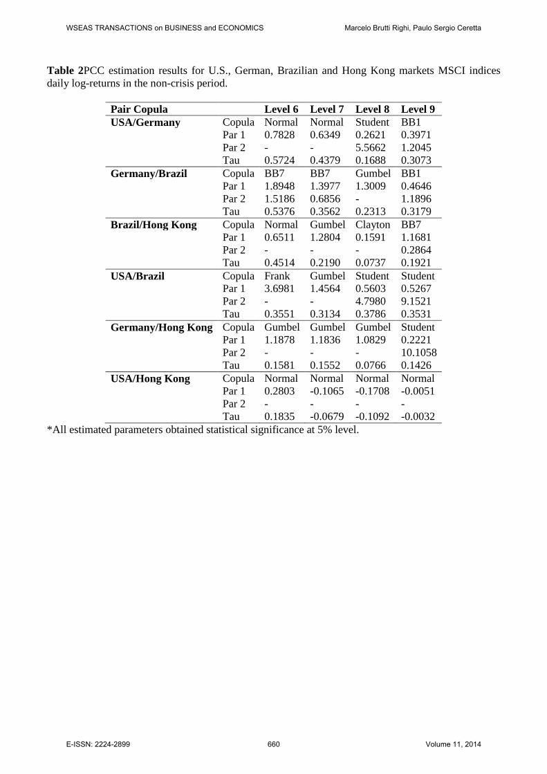
Table 2PCC estimation results for U.S., German, Brazilian and Hong Kong markets MSCI indices daily log-returns in the non-crisis period.

Pair Copula Level 6 Level 7 Level 8 Level 9 USA/Germany Copula Normal Normal Student BB1 Par 1 0.7828 0.6349 0.2621 0.3971 Par 2 - - 5.5662 1.2045 Tau 0.5724 0.4379 0.1688 0.3073 Germany/Brazil Copula BB7 BB7 Gumbel BB1 Par 1 1.8948 1.3977 1.3009 0.4646 Par 2 1.5186 0.6856 - 1.1896 Tau 0.5376 0.3562 0.2313 0.3179 Brazil/Hong Kong Copula Normal Gumbel Clayton BB7 Par 1 0.6511 1.2804 0.1591 1.1681 Par 2 - - - 0.2864 Tau 0.4514 0.2190 0.0737 0.1921 USA/Brazil Copula Frank Gumbel Student Student Par 1 3.6981 1.4564 0.5603 0.5267 Par 2 - - 4.7980 9.1521 Tau 0.3551 0.3134 0.3786 0.3531 Germany/Hong Kong Copula Gumbel Gumbel Gumbel Student Par 1 1.1878 1.1836 1.0829 0.2221 Par 2 - - - 10.1058 Tau 0.1581 0.1552 0.0766 0.1426 USA/Hong Kong Copula Normal Normal Normal Normal Par 1 0.2803 -0.1065 -0.1708 -0.0051 Par 2 - - - - Tau 0.1835 -0.0679 -0.1092 -0.0032

*All estimated parameters obtained statistical significance at 5% level.


E-ISSN: 2224-2899 660 Volume 11, 2014

Table 3PCC estimation results for U.S., German, Brazilian and Hong Kong markets MSCI indices daily log-returns in the sub-prime crisis period.

Pair Copula Level 6 Level 7 Level 8 Level 9 USA/Germany Copula Gumbel BB7 Student Student Par 1 2.2684 1.7891 0.3473 0.5279 Par 2 - 1.5037 2.7814 2.5340 Tau 0.5592 0.5254 0.2258 0.3540 Germany/Brazil Copula Joe BB7 BB1 BB1 Par 1 3.0759 2.2592 0.5696 0.5342 Par 2 - 1.6055 1.4112 1.5337 Tau 0.5292 0.5777 0.4485 0.4854 Brazil/Hong Kong Copula Normal BB7 Student BB7 Par 1 0.6368 1.3750 0.0772 1.2839 Par 2 - 0.8601 2.7780 0.3354 Tau 0.4395 0.3838 0.0492 0.2456 USA/Brazil Copula Clayton Frank Student Student Par 1 0.8131 3.8164 0.6060 0.5421 Par 2 - - 4.4680 3.3541 Tau 0.2890 0.3742 0.4145 0.3647 Germany/Hong Kong Copula Frank Student Gumbel Student Par 1 1.2130 0.3822 1.0985 0.2233 Par 2 - 4.4710 - 6.4083 Tau 0.1328 0.2496 0.0897 0.1434 USA/Hong Kong Copula Clayton Normal Frank Student Par 1 0.4967 -0.1818 1.7535 -0.1541 Par 2 - - - 7.2964 Tau 0.1989 -0.1164 0.1891 -0.0985



E-ISSN: 2224-2899 661 Volume 11, 2014

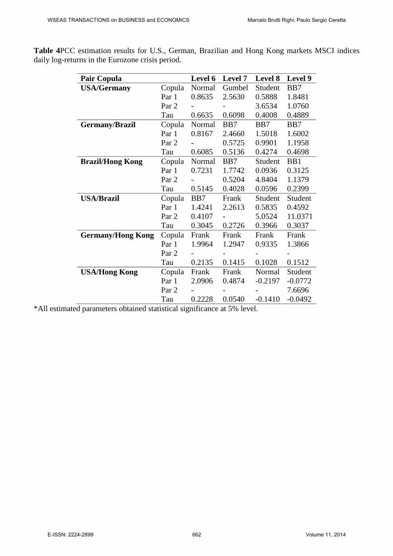
Table 4PCC estimation results for U.S., German, Brazilian and Hong Kong markets MSCI indices daily log-returns in the Eurozone crisis period.

Pair Copula Level 6 Level 7 Level 8 Level 9 USA/Germany Copula Normal Gumbel Student BB7 Par 1 0.8635 2.5630 0.5888 1.8481 Par 2 - - 3.6534 1.0760 Tau 0.6635 0.6098 0.4008 0.4889 Germany/Brazil Copula Normal BB7 BB7 BB7 Par 1 0.8167 2.4660 1.5018 1.6002 Par 2 - 0.5725 0.9901 1.1958 Tau 0.6085 0.5136 0.4274 0.4698 Brazil/Hong Kong Copula Normal BB7 Student BB1 Par 1 0.7231 1.7742 0.0936 0.3125 Par 2 - 0.5204 4.8404 1.1379 Tau 0.5145 0.4028 0.0596 0.2399 USA/Brazil Copula BB7 Frank Student Student Par 1 1.4241 2.2613 0.5835 0.4592 Par 2 0.4107 - 5.0524 11.0371 Tau 0.3045 0.2726 0.3966 0.3037 Germany/Hong Kong Copula Frank Frank Frank Frank Par 1 1.9964 1.2947 0.9335 1.3866 Par 2 - - - - Tau 0.2135 0.1415 0.1028 0.1512 USA/Hong Kong Copula Frank Frank Normal Student Par 1 2.0906 0.4874 -0.2197 -0.0772 Par 2 - - - 7.6696 Tau 0.2228 0.0540 -0.1410 -0.0492



E-ISSN: 2224-2899 662 Volume 11, 2014

wavelet - pair copula construction inference for financial ... · wavelet - pair copula...

Documents