Waveform discrimination analysis applied to

PoGOLino data

Victor Sedin

sedom@kth.se

SA104X Degree Project in Engineering Physics, First Level

Supervisor: Elena Moretti

Department of Physics

School of Engineering Sciences

KTH, Royal Institute of Technology

Stockholm, Sweden

May 21, 2013

Abstract

PoGOLite (Polarised Gamma-Ray Observer Lite) is a balloon borne experiment meantto measure the polarisation of the electromagnetic radiation from speci�c astrophysicalobjects. The main target of interest for PoGOLite is the Crab pulsar. A considerableparticle background was recorded during the short �ight of PoGOLite in July 2011. Inorder to further study the particle background before the relaunch of PoGOLite, a smallerexperiment named PoGOLino was initiated. For both experiments, methods to increasethe signal to noise ratio in the data collected are important. The aim of this project hasbeen to propose new methods for increasing the signal to noise ratio in collected data,and quantitatively compare them with the previous methods. On a data sample wherethe original ratio of signal to noise was 0.1, the prior methods were able to increase theratio to 1.13. A signal to noise ratio of 1.98 was achieved on the same data sample, whenexecuting two algorithms developed during the course of this project in sequence.

Contents

1 Introduction 2

2 Particle environment at high altitudes 4

2.1 PoGOLino goals . . . . . . . . . . . . . . . . . . . . . . . . . . . . . . . . 42.2 Cosmic ray interactions in the atmosphere . . . . . . . . . . . . . . . . . 42.3 Neutron environment at high altitude . . . . . . . . . . . . . . . . . . . . 6

3 PoGOLino 8

3.1 PoGOLino set up . . . . . . . . . . . . . . . . . . . . . . . . . . . . . . . 83.2 Detector description . . . . . . . . . . . . . . . . . . . . . . . . . . . . . 93.3 Read out electronics and logic . . . . . . . . . . . . . . . . . . . . . . . . 10

4 Methods of waveform discrimination 11

4.1 Previous work on waveform discrimination . . . . . . . . . . . . . . . . . 144.2 Analysis methods . . . . . . . . . . . . . . . . . . . . . . . . . . . . . . . 164.3 Selection of test samples . . . . . . . . . . . . . . . . . . . . . . . . . . . 16

5 Analysis description and application on data 18

5.1 Cut optimisation for fast waveform selection . . . . . . . . . . . . . . . . 185.1.1 Polished fast vs slow cut . . . . . . . . . . . . . . . . . . . . . . . 185.1.2 Peak vs area cut . . . . . . . . . . . . . . . . . . . . . . . . . . . 185.1.3 Negative slopes cut . . . . . . . . . . . . . . . . . . . . . . . . . . 19

5.2 Application of the selection algorithms . . . . . . . . . . . . . . . . . . . 205.3 Results . . . . . . . . . . . . . . . . . . . . . . . . . . . . . . . . . . . . . 24

5.3.1 Evaluation of spectra . . . . . . . . . . . . . . . . . . . . . . . . . 245.3.2 Application on test samples . . . . . . . . . . . . . . . . . . . . . 27

6 Conclusions 28

7 Appendix 29

7.1 Histograms of individually plotted radioactive isotopes . . . . . . . . . . 29

Bibliography 35

1

Chapter 1

Introduction

The study of astrophysical objects through measuring electromagnetic radiation has beenconducted for a long time, yet the polarisation has not been widely studied. Howevermany interesting astrophysical objects are expected to emit radiation with a high degreeof polarisation, as well as time and energy variations in the polarisation. Measurementsof the polarisation can be of value to evaluate the current models of these objects. PoGO-Lite (Polarised Gamma-Ray Observer Lite)1 is a balloon borne instrument for measuringpolarisation[1]. The main target to be observed during �ight is the Crab pulsar, a wellknown astrophysical object. At present there are three main models proposed for themechanism of electromagnetic emission from the Crab[2]. The expected intensity of theiremission is very similar. However, the expected polarisation di�ers between them. Mea-surements of the polarisation from PoGOLite will hopefully lead to a better understand-ing of pulsars of this kind. PoGOLite has been developed and built by a collaborationheaded by a team at KTH in Stockholm, Sweden[3].

A common problem for measurements in space is the large disturbance of the particlebackground, which consists of neutrons, charged particles and gamma-rays. During theshort �ight of PoGOLite in 2011, measurements con�rmed neutrons to be the dominantsource of background[4]. They also con�rmed that previous measurements regardingneutrons in the atmosphere at di�erent latitudes are not applicable to the conditions at40km altitude, 67◦ latitude which is the case when launching from Esrange (EuropeanSpace and Sounding Rocket Range) in Kiruna2.

In order to study these special conditions a small experiment called PoGOLino (Italianfor smaller PoGO) was initiated. The objective of the PoGOLino project is to measure theamount of particles as a function of the altitude, in preparation for the �ight of PoGOLite.On board PoGOLino there are detectors for neutrons as well as other particles, in aparticular con�guration that mimics that of PoGOLite. PoGOLino and PoGOLite bothuse scintillators to detect incoming particles. In order to distinguish between signal andbackground, di�erent kinds of scintillating materials are used, each with a characteristicdecay time. The analysis of the characteristic scintillator output signals called waveforms,makes active rejection of background possible.

PoGOLino was successfully launched in march 2013 and brought back unharmed afterdata was recorded[5]. it is important that e�ective tools are available for the current data

1�Lite� because it is a lighter version of a previously planned instrument. The �Gamma-Ray� part isbecause of historical reasons even though the instrument is meant to detect X-rays.

2Near the Swedish northern border.

2

analysis, hence the scope of this project has been to create and evaluate methods thatcan be useful for sorting waveforms depending on their characteristic times.Focus has been directed towards developing a waveform discrimination tool for dataoriginating from one of detectors on board PoGOLino. Similar detectors are used inPoGOLite, which makes results from the project applicable to the background rejectionanalysis of PoGOLite data.

The goals and data collection principles of PoGOLino are covered primarily in chap-ter 2, followed by an explanation of the particle environment at high altitude. Specialattention is given to explain the atmospheric conditions in the polar region due to theirsigni�cance for the project. In chapter 3 the relevant equipment and the choice of thedetector positions are described, as well as how the on board software works. The speci�cproblem of distinguishing between di�erent waveforms is described in detail in chapter 4,the chapter will also cover how this problem was dealt with prior to my work. Chapter 5contains the project results, and the methods introduced in chapter 4 are used to evaluatethe e�ectiveness of the analysis tools developed in the project. The conclusions of theproject are presented in chapter 6.

3

Chapter 2

Particle environment at high altitudes

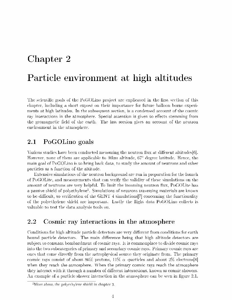
The scienti�c goals of the PoGOLino project are explicated in the �rst section of thischapter, including a short exposé on their importance for future balloon borne experi-ments at high latitudes. In the subsequent section, is a condensed account of the cosmicray interactions in the atmosphere. Special attention is given to e�ects stemming fromthe geomagnetic �eld of the earth. The last section gives an account of the neutronenvironment in the atmosphere.

2.1 PoGOLino goals

Various studies have been conducted measuring the neutron �ux at di�erent altitudes[6].However, none of them are applicable to 40km altitude, 67◦ degree latitude. Hence, themain goal of PoGOLino is to bring back data, to study the amount of neutrons and otherparticles as a function of the altitude.

Extensive simulations of the neutron background are run in preparation for the launchof PoGOLite, and measurements that can verify the validity of these simulations on theamount of neutrons are very helpful. To limit the incoming neutron �ux, PoGOLite hasa passive shield of polyethylene1. Simulations of neutrons traversing materials are knownto be di�cult, so veri�cation of the GENT 4 simulations[7] concerning the functionalityof the polyethylene shield are important. Lastly the �ight data PoGOLino collects isvaluable to test the data analysis tools on.

2.2 Cosmic ray interactions in the atmosphere

Conditions for high altitude particle detectors are very di�erent from conditions for earthbound particle detectors. The main di�erence being that high altitude detectors aresubject to constant bombardment of cosmic rays. It is commonplace to divide cosmic raysinto the two subcategories of primary and secondary cosmic rays. Primary cosmic rays areones that come directly from the astrophysical source they originate from. The primarycosmic rays consist of about 86% protons, 11% α -particles and about 2% electrons[8]when they reach the atmosphere. When the primary cosmic rays reach the atmospherethey interact with it through a number of di�erent interactions, known as cosmic showers.An example of a particle shower interaction in the atmosphere can be seen in �gure 2.1.

1More about the polyethylene shield in chapter 3.

4

Figure 2.1: Incoming primary cosmic rays interact with the atmosphere in a process called a cosmicshower. The particles resulting from the interactions are shown, this is one of many possible variationsof the cosmic showers. Reprinted from [9].

Secondary cosmic rays are the result of these cosmic showers. The amount of detectedparticles increase as the detector approaches the altitude where cosmic showers occur,and decreases once the detector has passed that altitude, as demonstrated in �gure 2.2.

Figure 2.2: The count of particles in the atmosphere as a function of pressure (solid curve) and ofaltitude (dashed curve). The maximum at around 20km is known as the Pfotzer peak. After the Pfotzerpeak the amount of particles detected falls o� quickly and stabilizes at around half of the peak value.Reprinted from [10].

5

This can be compared to �gure 2.3 depicting data collected during the short maidenvoyage of PoGOLite in 2011, which was aborted due to a helium leak. The Pfotzer peakcan be seen in these data as well, but appears at a di�erent altitude.

Figure 2.3: The �gure shows the particle count as a function of altitude in the data recorded byPoGOLite during the short �ight in 2011. The Pfotzer peak can be seen at about 30 kilometres altitude.Reprinted from[4].

As mentioned the primary rays consist mostly of charged particles, and as such theyare e�ected by the geomagnetic �eld, as illustrated in �gure 2.4.

If a charged particle comes in towards earth near the equator where the �eld linesof the geomagnetic �eld are directed tangentially to the earth surface, they will need tobe highly energetic not to be deviated by the magnetic �eld. Near the poles where themagnetic �eld is directed towards the earth's surface much less energetic primary cosmicrays will enter the atmosphere. The minimum energies required at di�erent locations fora particle to be able to pass the geomagnetic �eld barrier can be seen in �gure 2.5. Thegeomagnetic e�ect explains why data collected at other latitudes will not provide usefulinformation about the particle background environment when launching from Esrange,Kiruna.

2.3 Neutron environment at high altitude

PoGOLino will ascend to about 30km above sea level, a large part of the neutrons atthis altitude are created by cosmic showers. Although the resulting particles from theparticle showers have the highest probability to be emitted forward, they don't necessarilycontinue on the same direction as the original particle. Neutrons created in these showerscan be backscattered upwards, and thus particles originating from a lower altitude willalso hit the PoGOLino detectors from below.

The number of scattered neutrons is proportional to the amount of particles partakingin interactions in the atmosphere. Therefore more neutrons will be found at high latitudessuch as Kiruna, which has a low geomagnetic cut-o� energy, see �gure 2.5.

6

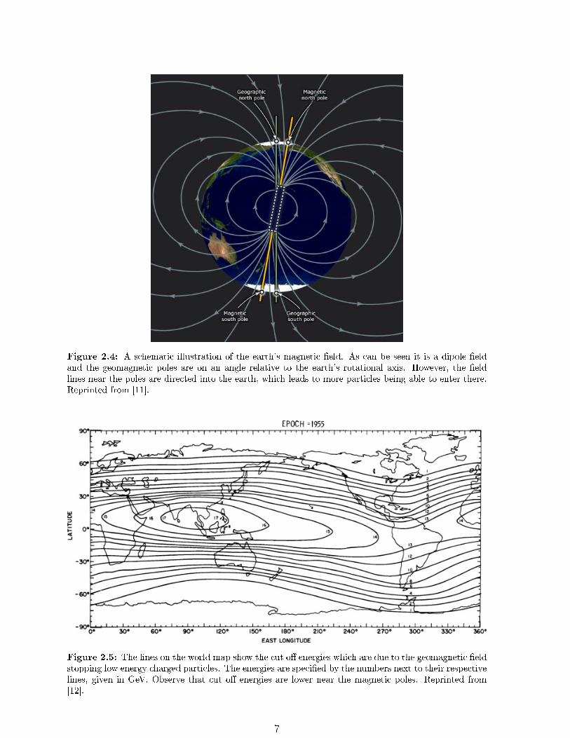
Figure 2.4: A schematic illustration of the earth's magnetic �eld. As can be seen it is a dipole �eldand the geomagnetic poles are on an angle relative to the earth's rotational axis. However, the �eldlines near the poles are directed into the earth, which leads to more particles being able to enter there.Reprinted from [11].

Figure 2.5: The lines on the world map show the cut o� energies which are due to the geomagnetic �eldstopping low energy charged particles. The energies are speci�ed by the numbers next to their respectivelines, given in GeV. Observe that cut o� energies are lower near the magnetic poles. Reprinted from[12].

7

Chapter 3

PoGOLino

3.1 PoGOLino set up

PoGOLino consists of an aluminium vessel closed by two end plates, inside of whichelectronics and detectors are mounted on four long metal rods. A large polyethyleneshield is screwed into place to one of the end plates, see �gure 3.1 for an overview ofPoGOLino with its case removed.

Figure 3.1: In the picture on the left PoGOLino can be seen with its protective case removed, on theright is a schematic of the equipment. The schematic is reprinted from [13]

As showed in �gure 3.1 there are two detectors placed inside the polyethylene shieldto register particles that pass through the shield. At the other side of the vessel there is aneutron detector as can be seen in �gure 3.1. This detector is not behind a polyethyleneshield. By analysing data from detectors with and without polyethylene around them,the e�ects of the polyethylene shield can be isolated.

8

3.2 Detector description

PoGOLino contains three PDCs (Phoswitch1 Detector Cells), each PDC consists of threescintillators layered in a sandwich con�guration. On one side the PDCs taper into acylinder which allows them to be tightly �tted against a PMT (Photomultiplier Tube)2.

Inside PoGOLino are two di�erent types of PDCs. The �rst kind is designed for neu-tron detection. The neutron detector is layered with a 5mm piece of LiCaAlF6 (LithiumCalcium Aluminium Fluoride) between two pieces of BGO (Bismuth Germanium Oxide,Bi4Ge3O12). The Lithium consists of 50% 6Li and 50% 7Li. The 6Li has a high neutroncapture cross section of 940barn, and is highly sensitive to thermal neutrons[14].

The other type of PDC is sensitive to di�erent kinds of particles, including X-raysand neutrons. However, contrary to the �rst type, the latter class of PDC does nothave high e�ciency for neutrons. This detector is layered with a 5mm thick �EJ-204�plastic[20] between two pieces of BGO. In the context of PoGOLino and PoGOLite theEJ-204 plastic scintillator is called the fast scintillator because of its short decay time of0.7ns.

As explained in chapter 3.1, one of the neutron detectors is covered by a polyethyleneshield. The purpose of this shield is to shift the energy spectrum of incoming neutrontowards lower energies. This is necessitated by the fact that high energy neutrons cannotbe distinguished from X-rays in the fast scintillator, unlike charged particles that depositmuch more energy in the scintillators and and are consequently recognised. Resultsfrom simulations of the e�ects of a 10cm polyethylene shield on an incoming neutronenergy spectrum are shown in �gure 3.2. The �gure illustrates how the shield has madeinteractions with the neutron scintillator more probable by shifting the energy spectrum.

Figure 3.2: Simulation results of the e�ects of the polyethylene shield on the energy spectrum ofincoming neutrons. The black line represents all the events that are registered. The red line representsthe neutrons initial energy, and the blue line represent their energy after traversing the polyethylene.Reprinted from [4], data taken from from[15].

1Short for Phosphor sandwich.2Model: Hamamatsu R7899EGKNP.

9

3.3 Read out electronics and logic

When an interaction excites the scintillator material in a PDC, light from the ensuingdeexcitations are registered by the PMT. The PMTs are connected to a FADC (FastAnalog to Digital Converter) board that handles the trigger logic, which is the decisionof which data to save. This logic is coded in VHDL3 (Virtual Hardware DescriptionLanguage) code. If between two clock cycles, the di�erence in ADC (Analog-to-DigitalConverter) channels is greater than a set value, a trigger is issued. When the trigger hasbeen issued 10 clock cycles before the trigger and 40 clock cycles after are recorded, hence50 clock cycles of data are collected which constitutes a waveform. Events with energyexceeding a set threshold are vetoed. This process is executed during data collection, andis therefore called the online analysis as opposed to the consecutive o�ine addressed inthis project. The online analysis is necessitated by an otherwise unsustainable demandon data storage.

3Developed at Hiroshima by Hiromitsu Takahashi with assistance of Takafumi Kawano, TakzumiHirano and Merlin Kole.

10

Chapter 4

Methods of waveform discrimination

This chapter will begin by introducing the terminology thus far unde�ned followed by anaccount of the importance of dependable methods for waveform discrimination. Section4.1 introduces the hitherto utilised methods for waveform discrimination. The two suc-ceeding sections introduce tools for the evaluation of waveform discrimination methods.

From now on the EJ-204 plastic scintillator will be referred to as the fast scintillator,and the waveforms resulting from interactions in this material will be referred to as fastwaveforms. The waveforms resulting from interactions in the BGO will be referred to asslow waveforms. Algorithms created to remove noise from the data will be referred to ascuts.

Since the online analysis which was introduced in section 3.2 is applied simultaneouslyas data is being collected it must be fast and therefore cannot be too sophisticated. Forthis reason data that has passed the �rst sorting the online analysis will contain undesiredwaveforms. Further re�nement is accomplished by the o�ine analysis, which works withdata already processed by the online analysis. The purpose of the o�ine analysis is toincrease the signal-to-noise ratio of the data, without the time constrains of the onlineanalysis.

Di�erences in the scintillator materials lead to di�erently shaped waveforms. The fastwaveform has a rise time of ∼ 0.1µs, while the rise time of the slow waveform is ∼ 0.3µs,which is illustrated in �gure 4.1.

The di�erence in rise times is utilised by the o�ine analysis, which distinguish betweensignals on the basis of the shape of their waveforms. Figure 4.2 depicts a fast waveform,the kind of waveform that constitutes the signal and which the o�ine analysis will try todistinguish. If the o�ine analysis is e�ective, there will be a higher prevalence of thesewaveforms as opposed to background than in the original data. For comparison a slowwaveform can be seen in �gure 4.3.

Another kind of waveforms of relevance because of its high prevalence in PoGOLinodata is the superimposed waveform, which occurs when both the BGO and the fastscintillator are excited within one CPU (Central Processing Unit) clock cycle. Equation(4.1) shows that light travels the 5mm between the layers in the PDCs in much less timethan one clock cycle of the CPU onboard PoGOLino1.

T =1

f= {f = 37.5MHz} =

1

37.5 ∗ 106≈ 27ns (4.1)

1Light travels 5mm through a material with re�ective index n in ≈ n∗5∗10−3m2,997∗108 m

s≈ n*0.017ns, which

for any relevant(or realistic) n is much less than 27ns.

11

Figure 4.1: The fast plastic scintillator has a shorter rise time than the BGO. In this plot the polarityis negative[16]. Reprinted from [17].

Where T is the time of one clock cycle, and f is the frequency of the CPU (37.5Mhz). Soif a photon interacts with the BGO and then travels to the fast scintillator and interactswith it, then a fast waveform will be superimposed on a slow one. An example of asuperimposed waveform can be seen in �gure 4.4.

Figure 4.2: A fast waveform, these are the waveforms the o�ine analysis will try to single out. Thisexample is fairly clean, as can be seen by the rather smooth shape of the curve.

12

Figure 4.3: The �gure shows a slow waveform, resulting from an interaction in the BGO. This exampleis also fairly clean, as can be seen by the rather smooth shape of the curve.

Figure 4.4: A superimposed waveform, here both types of material in a PDC have been excited withinthe duration of a single clock cycle.

13

4.1 Previous work on waveform discrimination

Previous to this project a continuous e�ort has been made to improve the o�ine analysis.The most used method is based on two values, called the fast output and slow output.These values are calculated as in equations (4.2) and (4.3) [17]:

Fast output = max1≤i≤46

{v[i+ 4]− v[i]} (4.2)

andSlow output = max

1≤i≤35{v[i+ 15]− v[i]} (4.3)

Where v[i] is the amplitude of the waveform in the i:th sample point, 1 ≤ i ≤ 50. Inthis section it is important to know that in PoGOLite more data points are saved beforethe trigger. The principles are the same, but the sample point numbering is altered forPoGOLino.

Once these fast outputs and slow outputs are calculated the events can be plotted ina histogram, see �gure 4.5.

Waveforms that look alike will cluster together in the histogram branches. Eventscan be selected depending on whether or not they satisfy equation (4.4).

kl1 ∗ Fast output +ml1 < Slow output < kl2 ∗ Fast +ml2 (4.4)

Where l ∈ N and kl1, kl1,ml1,ml2 are constants di�erently set for the upper and lowerboundaries of the l:th section of the histogram. The dotted blue and red lines in �gure4.5 show two areas that satisfy equation (4.4) with the constants set the following way[17]: k11 = 1.0, m11 = −40, k12 = 1.0, m12 = 140, k21 = 2.1, m21 = −300, k22 =2.8, m21 = 100. Notice that when using equations (4.2) and (4.3) both the slow and fastoutput will equal similar values in the fast waveforms 2. Which is why the fast branchcan be seen to have a 1-to-1 inclination in �gure 4.5.

The method has been re�ned after the realisation that better separation is achievedwhen the slow output is commenced from the same data point as the fast output. Meaningthat the fast output is �rst calculated with equation (4.2) after which the slow output iscalculated with equation (4.5)

Slow output = v[j + 15]− v[j] (4.5)

where : j = i if and only if v[j + 4]− v[j] = max1≤i≤46

{v[i+ 4]− v[i]}

where i and j are data points, and v[k] is the amplitude in the k:th data point.Increased separation of the histogram branches could be seen when the cut was appliedon data after these modi�cations. In spite of the work done so far on the waveformanalysis, the members of PoGOLite collaboration are of the opinion that it is desirableto further improve the waveform analysis.

2Because both the slow output and the fast output will use the data point corresponding to thehighest eligible value of the waveform as their second value, and the baseline as their �rst

14

Figure 4.5: Events are plotted in a histogram depending on their fast output and slow output. Thered dotted lines de�nes what events survive the cut (These data are from PoGOLite and slow scintillatorrefers to a type of plastic scintillator not used in PoGOLino). Reprinted from [17].

15

4.2 Analysis methods

In order to �nd the optimal cut, it is necessary to �nd a systematic way of evaluatingthe e�ectiveness of cuts. In this section the tools used and the principles followed whenevaluating new cuts will be covered.

A useful tool is data from irradiation of PDCs by a known radioactive source in alaboratory environment. The reason being that the signal portion of this data can beknown beforehand. So since the purpose of a cut is to remove background, it can be knownbe known beforehand what would be sorted as signal in a �awless cut. The e�ectivenessof a cut can be evaluated by its approval rate of data and how well this performanceapproximates the calculated values of radioactive signal and background, respectively.The way to control this is to plot a spectrum in the form of a histogram, where thenumber of waveforms with speci�c peak amplitude is plotted against the ADC-value ofthe waveform peak.

Numerous such data �les were recorded, measuring di�erent radioactive isotopes tomake sure that the speci�c energies are not important for the e�ectiveness of the algo-rithms.The used radioactive sources and their characteristic emission peaks are given intable 4.1, and how the plastic scintillator interacts with the photons of di�erent energiesis shown in �gure 4.6.

Element Isotope γ emission E (keV)Cesium Cs-137 ∼ 660Cobalt Co-60 ∼ 1173, 1333Sodium Na-22 ∼ 511, 1022, 1274

Table 4.1: Table of the names and emission energies for the radioactive sources that were used to makedata samples for the analysis.

With the information from 4.1, and the material properties of the EJ-204 plasticscintillator, which are shown in �gure 4.6 it can be predicted what forms of interactionswill occur in the scintillator when it is irradiated by a speci�c radioactive source.

Histograms check the separation between branches of data after each cut is applied.A good cut will have a large separation between the branches populated by fast or slowwaveforms and preferably have the signal events placed closely together. Furthermoreeach cut was tested on two test samples, one of signal only and one of background only,which will be introduced in the next section.

4.3 Selection of test samples

Themain quantitative evaluation of the e�ectiveness of cuts was to apply them to two testsamples, consisting of manually sorted waveforms. In order to create these test samplesseveral thousands of waveforms were checked one by one. The clean fast events weresaved to one data �le, and the background waveforms were saved into another data �le.To reduce the human factor the data was re-sorted repeatedly, and an increasing rate ofbackground was discarded each time. To get waveforms from a wide energy range, andin order to remove systematic errors this process was employed on data samples fromdi�erent radioactive isotopes. The data �les were then put together to what was the

16

Figure 4.6: Mass attenuation coe�cient for photon interactions in the EJ-204 plastic scintillator. Base�gure reprinted from [17], with data from [18].

�nal, clean and background test samples. The �nal sample with signal contained 1000waveforms, and the �nal background sample contained 10,000 waveforms. If an idea fora cut did not perform well on the test samples it was disquali�ed.

17

Chapter 5

Analysis description and application on

data

In this chapter, the algorithms developed during the course of this project, and resultsfrom when the algorithms are applied to data are presented. In section 5.1 the algorithmsare de�ned and outlined in detail. In section 5.2 the algorithms are applied to di�erentsets laboratory data. Lastly, in section 5.3 the algorithms are evaluated by the methodsintroduced in sections 4.2 and 4.3 to produce the �nal results of this project.

5.1 Cut optimisation for fast waveform selection

5.1.1 Polished fast vs slow cut

This project has used equations (4.2) and (4.5) to determine the fast output and slowoutput. An extra restriction was added, the fast output must correspond to i = 10 ± 2in equation (4.2). If an event satis�es this condition, then the event continues to thenext step of the analysis, otherwise it is discarded. This restriction proved useful and istherefore implemented in all cuts. Any results achieved in this project will be evaluatedin comparison to the results achieved by this version of the fast vs slow cut.

5.1.2 Peak vs area cut

This algorithm works by �rst calculating the peak ADC, as de�ned in equation (5.2),

Peak := j where j satisfies v[j]− v[j − 4] = max1≤i≤46

{v[i+ 4]− v[i]} (5.1)

Peak ADC := v[j] with j as in equation (5.1) (5.2)

Where i, j ∈ N , i, j ≤ 50 and v[k] is the amplitude of the waveform at the k:th clockcycle. Thereafter it calculates the integral from equation (5.3) on page 18 which goesfrom the peak (as de�ned in equation (5.1)) until the end of the waveform.

Area =

∫ t2

t1

v(t)dt (5.3)

18

Where v(t) is measured in ADC channels and t is time. The set value t1 is the time ofthe peak and t2 the time at the end of the waveform. Waveforms are then classi�ed assignal or background depending on how the peak ADC and the magnitude of the areaare related. The integral in equation (5.3) is numerically calculated with Root[19], adata analysis framework for C++, developed at CERN (Organisation Europeenne pourla Recherche Nucleaire, previously Conseil Europeen pour la Recherche Nucleaire).

The concept of the peak vs area cut can be understood by examining �gure 5.1.Where the purple dot indicates the peak, and the red area indicates the area as de�nedby the area in equation (5.3). For fast waveforms the number of ADC-channels at thepeak is large, and the area is small, for slow waveforms it is the opposite.

Figure 5.1: In this �gure the peak is marked by a purple circle, and the integral calculated fromthe peak to the end of the waveform is marked by the red area. The di�erence between the waveformamplitude at the peak, as well as the di�erence in size of the area between the two waveforms can easilybe seen.

Observe that even though the peak ADC value corresponds to the highest amplitudeof a fast waveform, it is not necessarily the case for other waveforms. For BGO forexample, the value is taken when the waveform has reached about half of its maximumvalue.

5.1.3 Negative slopes cut

This algorithm utilises the fact that a fast waveform will have a certain number of negativeamplitude changes between two consecutive clock cycles. If there are more or less, it iseither a di�erent kind of waveform or a sign that something out of the ordinary hasoccurred. More precisely, the algorithm calculates the sum in equation (5.4).

Neg =49∑i=0

qi where

{qi = 1 if (v[i+ 1]− v[i]) < a

qi = 0 if (v[i+ 1]− v[i]) ≥ a(5.4)

Where a is a chosen number of ADC channels, and v[i] is the amplitude at the i:th datapoint. After evaluation of di�erent cut limits, it was concluded that demanding neg>33for fast waveforms was optimal. When that is set as the cuto� limit, this cut is calledthe neg>33 cut.

19

5.2 Application of the selection algorithms

In this section histograms with events plotted versus the cut variables for the algorithmsintroduced in the preceding section are shown. The data consists of several laboratorysamples of the radioactive isotopes displayed in table 4.1 on page 16 merged together.By inspecting the histograms one can see that the cuts are not a�ected by the energiesof the photons that induced the waveforms. To see the histograms for each isotopeindividually, see the appendix. Because waveforms with a similar appearance will havea similar relationship between their cut variables they will cluster together in distinctpopulations referred to as branches when plotted in the aforementioned histograms.

A histogram with the fast output on the horizontal axis and the slow value on thevertical axis is displayed in �gure 5.2. The fast branch containing the waveforms originat-ing from the plastic scintillator have gathered in the population which has been isolatedin �gure 5.3, by using equation (4.4). There are two other distinct branches. The slowbranch with a slow output about two times as larger its fast output containing slowwaveforms originating from the BGO. And then there is the branch between the slowand the fast branch, which contains the superimposed waveforms.

Figure 5.2: Data from the di�erent radioactive isotopes merged together. The events are plotteddepending on their fast output and slow output. This illustrates how the peak vs area cut distinguishesbetween waveforms. As can be seen the peak vs area cut is not a�ected by the fact that the data comesfrom waveforms from a wide energy range.

The histogram for the peak vs area cut, with the peak ADC value on the horizontalaxis and the area on the vertical axis is shown in �gure 5.4. The branches of data arethe same as for the fast vs slow cut, and as with the fast vs slow cut there is no problemwith the wide energy range of the data set. But the signal contain fewer events, as canbe seen by the number of entries in the data displayed in �gure 5.5. In the next sectionresults that show that the reduced number of signal events according to the peak vs arecut compared with the fast vs slow cut is due to increased background rejection and notbecause of reduced signal recognition.

Lastly, the same three populations can be seen in �gure 5.6 on page 23, with the slowwaveforms having the fewest number of negative slopes (count peaking at 13 negative

20

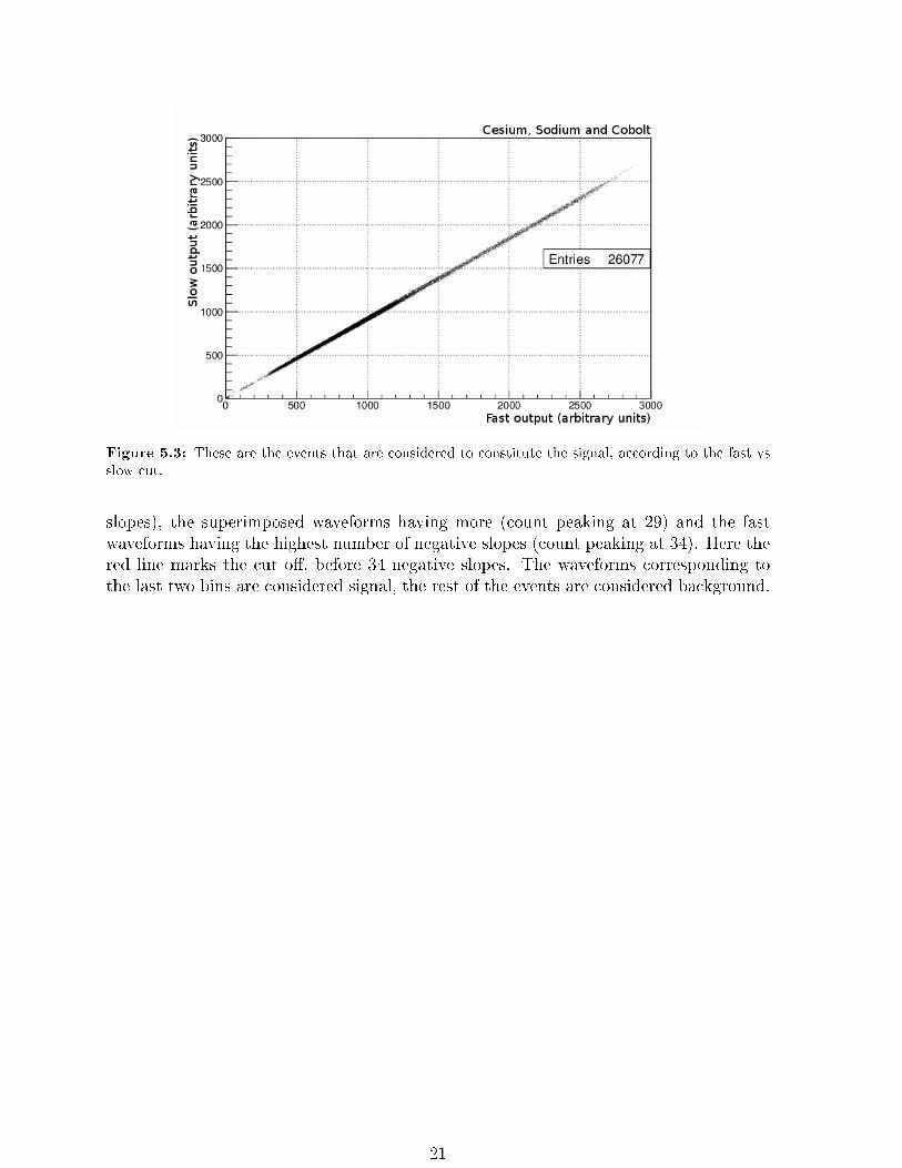
Figure 5.3: These are the events that are considered to constitute the signal, according to the fast vsslow cut.

slopes), the superimposed waveforms having more (count peaking at 29) and the fastwaveforms having the highest number of negative slopes (count peaking at 34). Here thered line marks the cut o�, before 34 negative slopes. The waveforms corresponding tothe last two bins are considered signal, the rest of the events are considered background.

21

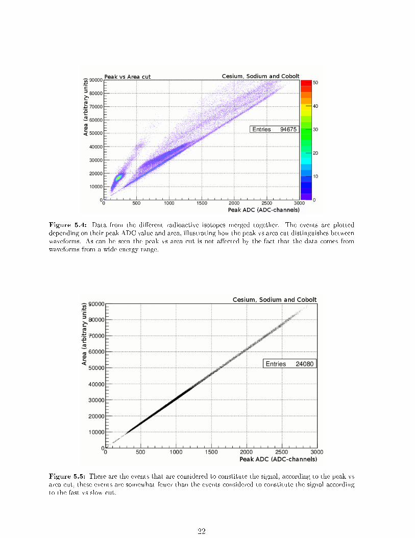
Figure 5.4: Data from the di�erent radioactive isotopes merged together. The events are plotteddepending on their peak ADC value and area, illustrating how the peak vs area cut distinguishes betweenwaveforms. As can be seen the peak vs area cut is not a�ected by the fact that the data comes fromwaveforms from a wide energy range.

Figure 5.5: These are the events that are considered to constitute the signal, according to the peak vsarea cut, these events are somewhat fewer than the events considered to constitute the signal accordingto the fast vs slow cut.

22

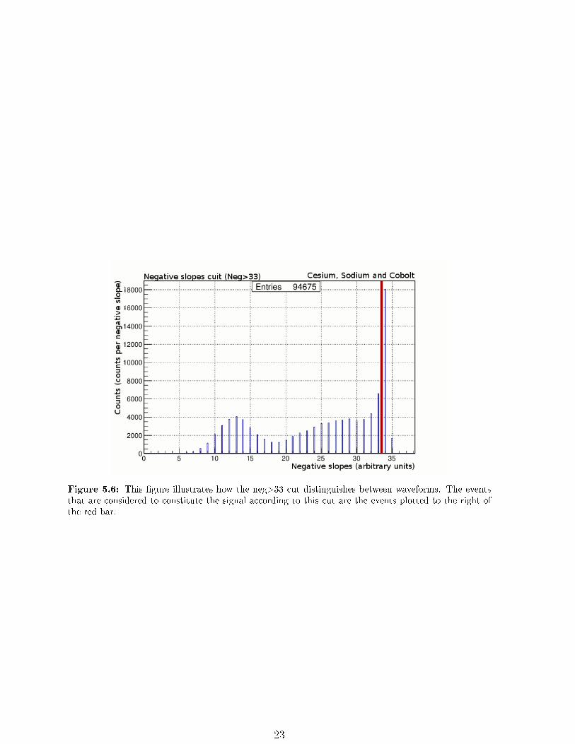
Figure 5.6: This �gure illustrates how the neg>33 cut distinguishes between waveforms. The eventsthat are considered to constitute the signal according to this cut are the events plotted to the right ofthe red bar.

23

5.3 Results

5.3.1 Evaluation of spectra

This section compares histograms with event count plotted versus peak ADC values. Inthe cases when no cut (except for the demand that the trigger is located in clock cyclei = 10± 2) has been applied to the data, the histograms can look suspicious with largepeaks at low ADC values. However the de�nition of the peak ADC (see equation (5.2))correspond to the highest ADC-value for fast waveforms, but not necessarily for otherwaveforms. Therefore the spectra can not be interpreted before the cuts for backgroundreduction are applied to the dataset.

Sodium

From 22Na the emission peaks are 511 keV, 1022 keV and 1274 keV. The amount ofphotons emitted corresponding to the �rst peak is signi�cantly more than the othertwo peaks. As shown in �gure 4.6 on page 17, the plastic scintillator will interact withphotons with either of these energies through Compton scattering[21]. Because there isa signi�cantly larger amount of BGO than plastic scintillator, and because BGO has alarger cross section for interaction with photons of these energies[18] a large portion ofthe data will originate from the BGO and consist of background. Therefore an e�ectivecut will remove most of the background events in the data, and the histogram shouldshow a smooth curve peaking at an ADC-value corresponding to 511 keV. The smoothslope is to be expected because of the angular dependence of the kinetic energy for theCompton scattered electrons.

It is quite easy to qualitatively say from inspecting �gure 5.7 that all the cuts increasethe signal to noise ratio, however it appears that the neg>33 cut does the best job, whilethe fast vs slow cut and the peak vs area cut are more comparable, even if the peak vsArea cut seems to be somewhat more e�ective.

Cesium

Since the emission peak for 137Cs is at 662 keV the photons will interact with the plasticscintillator through Compton scattering. Therefore the histograms for 137Cs, if a cut ise�ective, is quite similar to the 22Na, except for where the slope should peak, and sincethere is no other emission peak with a higher energy there should be no signi�cant amountof events at higher ADC values than where the peak is located. These expectations canbe controlled by inspection of �gure 5.8.

Since the two peaks at lower ADC-channels are removed by all the cuts, they all seemto be e�ective at removing background. But as was seen in the sodium histograms, theneg>33 cut seems to give a histogram with the most even slope, and with the most eventsremoved. Once again the shapes achieved after applying the fast vs slow and peak vsarea cuts are very similar.

24

Figure 5.7: The four histograms show data after four di�erent cuts have been applied. Sodium emitsmostly 511 keV photons, but also 10022 keV and 1274 keV photons which are outside of the energy rangeof the equipment. A perfect cut would show a large, smooth slope with its peak at around 900ADC(crosschecked with Cesium data), and then a smaller amount of events up to the ADC limit. The neg>33 cutgives a result which looks much like that, followed by the peak vs area cut and then the fast vs slow cut.

25

Figure 5.8: The four histograms represent the data from laboratory irradiation with Cesium, after fourdi�erent cuts have been applied. Because of the single gamma emission energy of 662 keV of the Cesiumit easy to predict how signal should appear in the histograms. A smooths slope from Compton scatteredevents, peaking at around 1100ADC-channels (cross checked with Sodium) should appear. The bump inthe slope seen in these histograms, after the cuts have been applied seem to indicate that there is roomfor some optimisation regarding how the branch distinctions are drawn. However the result indicatesthe same order of e�ectiveness among the cuts. With the neg>33 cut providing the best result, followedby the peak vs area cut and then the fast vs slow cut.

26

5.3.2 Application on test samples

The selection algorithms were applied one by one to the test samples introduced in section4.3, and the results can be seen in table 5.1.

Cut Nothing Fast vs Slow Peak vs Area neg>33Signal 1000 974 932 909

Background 10,000 860 784 532Ratio 0.1 1.13 1.19 1.71

Table 5.1: The table shows the ratio between signal and background when no cuts are applied andwhen the studied cuts are applied. In each column the number of signals that passed the cut (truepositive) and the number of background waveforms that passed cut (false positive) are listed.

The algorithms were applied then in combination to the test samples, and the resultsin table 5.2 were achieved.

Cut Nothing Fast vs Slow and neg>33 Peak vs Area and neg>33Signal 1000 893 849

Background 10,000 457 428Ratio 0.1 1.95 1.98

Table 5.2: The table shows the results obtained when the cuts were applied in combination to thetests samples. As can be seen, the resulting signal to noise ratio was higher when the cuts were run incombination, particularly the neg>33 combined with the Peak vs Area cut achieved the highest signalto noise ratio.

It is clear from the results that a better signal to noise ratio is achieved when thealgorithms are run in combination, and also that the algorithms developed during thecourse of this project give a higher signal to noise ratio, compared with the algorithmused before. These results are in line with the results shown in section 5.3.1.

27

Chapter 6

Conclusions

The PoGOLite experiment will give a deeper understanding of astrophysical objects, pri-marily the Crab nebula and Crab pulsar. The theoretical models of how the Crab pulsaremits electromagnetic radiation have distinctly di�erent predictions for the polarisation.The imminent PoGOLite polarimetry may come to conclude which theoretical model iscorrect.

The predicted severe particle background at �ight altitude of PoGOLite was con�rmedduring the short �ight of PoGOLite in 2011, which prompted the PoGOLino projectwhose purpose is to retrieve experimental data to further study the environmental particlebackground. PoGOLino was successfully launched in March 2013 and the data retrievedat its return is currently being analysed.

Much like PoGOLite, PoGOLino uses scintillator detectors with di�erent decay timesto actively reject background. If a particle interacts with the detector dedicated to signaldetection a fast waveform is produced. On the contrary if a particle interacts with thescintillator dedicated to background rejection a slow rising waveform is produced.

The ability to e�ectively di�erentiate between waveforms is a crucial part of thedata analysis of both PoGOLino and PoGOLite, and the scope of this project has beento improve that process. During the course of this project a number of new selectionmethods have been developed to distinguish between signal and background.

It could be concluded that all of the selection methods increased the signal-to-noiseratio when applied to laboratory irradiation data from radioactive samples. Howeverthe new methods proposed seemed to improve the signal to noise ratio more than thepreviously adopted methods.

Application of all the selection methods to a pure signal sample and a pure backgroundsample, con�rmed an improvement respect to the method previously adopted by thePoGOLite collaboration.

The new proposed methods, the peak vs area cut and the neg>33 cut raised thesignal-to-noise ratio of the test samples from 0.1 to 1.19 and 1.71 respectively. Whenrun in combination they achieved a signal-to-noise ratio of 1.98, these results were animprovement over the signal-to-noise ratio of 1.13 achieved when applying the fast vsslow cut which is the currently used method.

Excitingly PoGOLino was launched during the fabrication of this thesis, and on thataccount the proposed continuation is to test the selection methods of this project on thedata collected during the �ight of PoGOLino. After that an interesting extension wouldbe to test the methods on data from PoGOLite.

28

Chapter 7

Appendix

7.1 Histograms of individually plotted radioactive iso-

topes

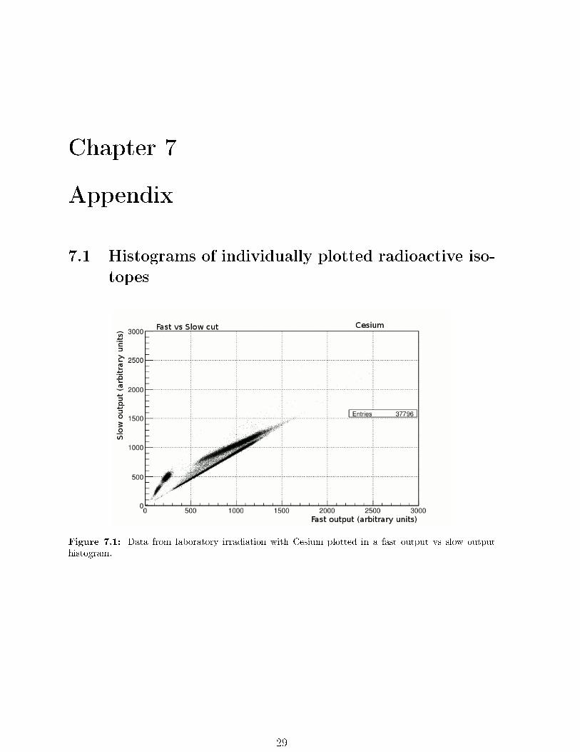
Figure 7.1: Data from laboratory irradiation with Cesium plotted in a fast output vs slow outputhistogram.

29

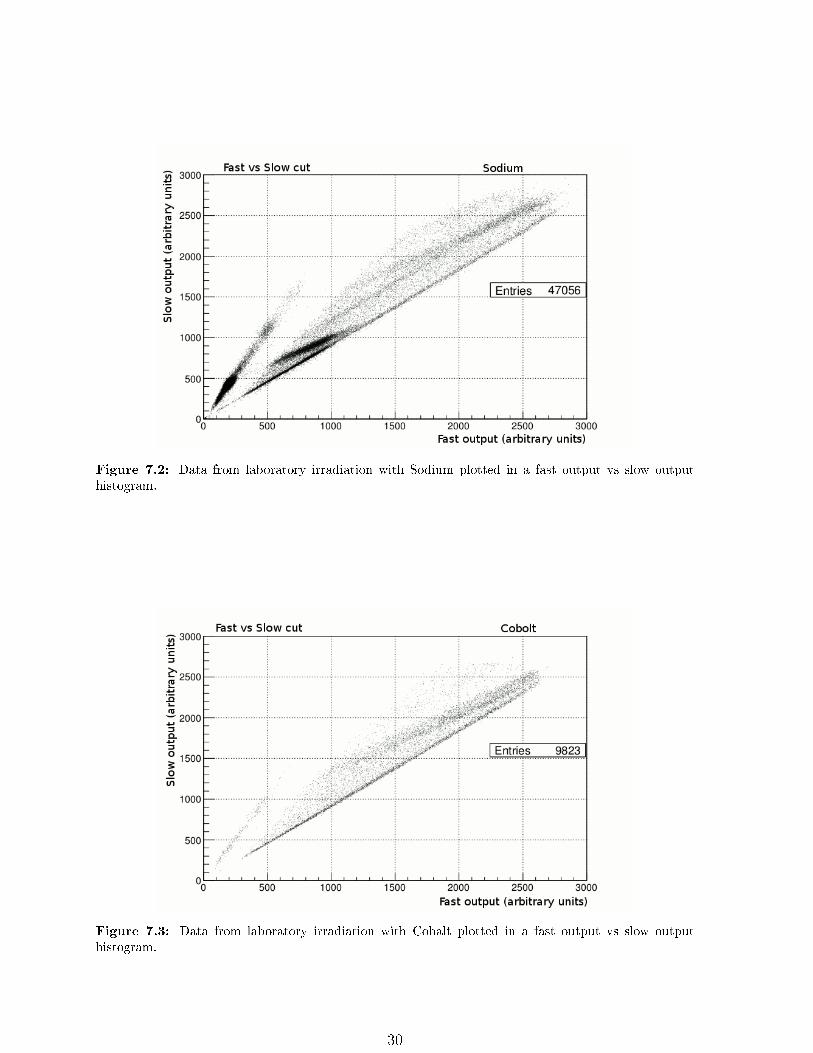
Figure 7.2: Data from laboratory irradiation with Sodium plotted in a fast output vs slow outputhistogram.

Figure 7.3: Data from laboratory irradiation with Cobalt plotted in a fast output vs slow outputhistogram.

30

Figure 7.4: Data from laboratory irradiation with Cesium plotted Peak ADC-channels versus areahistogram.

Figure 7.5: Data from laboratory irradiation with Sodium plotted in a Peak ADC-channels versus areahistogram.

31

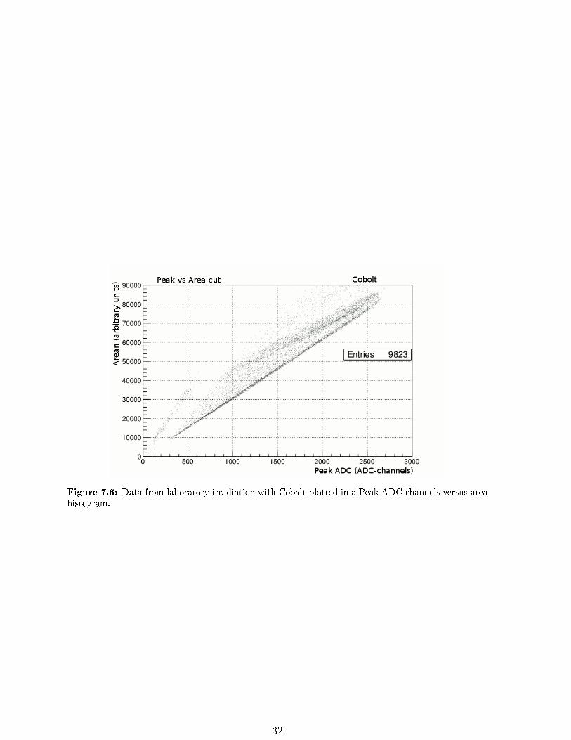
Figure 7.6: Data from laboratory irradiation with Cobalt plotted in a Peak ADC-channels versus areahistogram.

32

List of Figures

2.1 One of many kinds of particle shower interactions. . . . . . . . . . . . . . 52.2 Data which shows a clear Pfotzer peak. . . . . . . . . . . . . . . . . . . . 52.3 PoGOLino particle count rate data from the 2011 �ight. . . . . . . . . . 62.4 Schematic illustration of the geomagnetic �eld. . . . . . . . . . . . . . . . 72.5 Geomagnetic cut o� energies drawn on map of the earth. . . . . . . . . . 7

3.1 Photograph of PoGOLino placed next to a schematic of PoGOLino. . . . 83.2 Simulated energy spectrum of neutrons, before and after polyethylene. . . 9

4.1 Rise times of BGO and the fast scintillator in one common plot. . . . . . 124.2 A fast waveform. . . . . . . . . . . . . . . . . . . . . . . . . . . . . . . . 124.3 A BGO waveform. . . . . . . . . . . . . . . . . . . . . . . . . . . . . . . 134.4 A superimposed waveform. . . . . . . . . . . . . . . . . . . . . . . . . . . 134.5 Events plotted in a histogram based on their fast output and slow output. 154.6 Events plotted in a histogram based on their fast output and slow output. 17

5.1 Illustration that explains the peak vs are cut. . . . . . . . . . . . . . . . 195.2 Events plotted in a histogram based on their fast output and slow output. 205.3 Signal events according to the fast vs slow cut, from the three radioactive

isotopes together. . . . . . . . . . . . . . . . . . . . . . . . . . . . . . . . 215.4 Events plotted in a histogram based on their fast output and slow output. 225.5 Signal events according to the peak vs area cut, from the three radioactive

isotopes together. . . . . . . . . . . . . . . . . . . . . . . . . . . . . . . . 225.6 A histogram for the neg>33 cut, with events from the data �le with the

three radioactive samples placed together. . . . . . . . . . . . . . . . . . 235.7 Four histograms of counts per bin versus peak ADC, displaying data from

laboratory irradiation with Sodium. . . . . . . . . . . . . . . . . . . . . . 255.8 Four histograms of counts per bin versus peak ADC, displaying data from

laboratory irradiation with Cesium. . . . . . . . . . . . . . . . . . . . . . 26

7.1 Histogram plotted with Cesium data, axis: Fast and Slow. . . . . . . . . 297.2 Histogram plotted with Sodium data, axis: Fast and Slow. . . . . . . . . 307.3 Histogram plotted with Cobolt data, axis: Fast and Slow. . . . . . . . . . 307.4 Histogram plotted with Cesium data, axis: Peak ADC-channels and Area. 317.5 Histogram plotted with Sodium data, axis: Peak ADC-channels and Area. 317.6 Histogram plotted with Cobolt data, axis: Peak ADC-channels and Area. 32

33

List of Tables

4.1 Information about sources used for laboratory tests. . . . . . . . . . . . . 16

5.1 Results from when cuts were applied one by one to the test samples. . . . 275.2 Results from when cuts were applied in combination to the test samples. 27

34

Bibliography

[1] M. Pearce, M. Kiss, �PoGOLite: Opening a new window on the Universe withpolarised gamma-rays�, Proceedings of �Imaging 2006�, Stockholm, June 2006.

[2] J. Dyks, et al, �Relativistic E�ects and Polarization in Three High-Energy PulsarModels�, Astrophysical Journal 606:1125-1142, May 2004.

[3] �The PoGOLite collaboration website�, http://www.particle.kth.se/

pogolite/, Accessed, 31 March 2013.

[4] M. Kole, �PoGOLite: 2011 �ight results and 2012 pre-�ight predictions�, LicentiateThesis 2012.

[5] Oscar Clein Center's website, http://okc.albanova.se/blog/

pogolino-successfully-launched/, Accessed 31 march 2013.

[6] �Altitude and Latitude Variations in Avionics SEU and Atmospheric Neutron Flux�,IEEE TRANSACTIONS ON NUCLEAR SCIENCE VOL. 40, NO. 6 DECEMBER1993.

[7] The Geant 4 toolkit website, http://geant4.cern.ch/, Accessed 18 May 2013.

[8] D.H Perkins, Particle Astrophysics, 2nd edition, section 6.1, page 148, Particle andAstrophysics department, Oxford University, ISBN: 0198509529.

[9] �Sciencenews� homepage, special credit to E. Feliciano, http://www.sciencenews.org/view/access/id/341881/description/PARTICLE_SHOWER/, with originalimage taken from http://imagine.gsfc.nasa.gov/docs/science/know_l1/

cosmic_rays.html, Accessed, 31 march 2013.

[10] G. Pfotzer, Z. Physik 102, 23, 1936.

[11] T. Hurst, �Magnetic �eld - The magnetic �eld and its direction�, Te Ara - theEncyclopedia of New Zealand, updated 14-Nov-12�,http://www.TeAra.govt.nz/en/diagram/9213/earths-magnetic-field Accessed 14 april 2013, base imagetaken from http://visibleearth.nasa.gov/.

[12] D.F. Smart, M.A. Shea, �Fifty years of progress in geomagnetic cuto� rigid-itydeterminations�, D.H Perkins, Advances in Space Research, Volume 44, Issue 10,November 16 2009.

[13] M.Kole, �PoGOLino�, PoGOLite collaboration internal document, available upon

request, April 2013

35

[14] H. Takahashi et al, �A Thermal-Neutron Detector with a Phoswich System ofLiCaAlF6 and BGO Crystal Scintillators on board PoGOLite�, As presented at

the IEEE conference 2011.

[15] T.W Armstrong et al, �Calculations of Neutron Flux Spectra Induced in the EarthsAtmosphere by Galactic Cosmic Rays", Journal of Geophysical Research, 1973.

[16] T. Tanaka et al, �Data Acquisition System for the PoGOLite Astronomical HardX-ray Polarimeter�, Nuclear Science Symposium Conference Record, (2007) 445.

[17] M. Kiss, �Pre-�ight development of the PoGOLite Path�nder�, PhD thesis, April2011.

[18] M.J. Berger, et al, �National Institute of Standards and Technology XCOM: Pho-ton Cross Sections Database� http://www.nist.gov/pml/data/xcom/index.cfm,Accessed May 20 2013.

[19] Root homepage, http://root.cern.ch/drupal/, Accessed 23 April 2013.

[20] EJEN Technology product data sheet, http://www.eljentechnology.com/

images/stories/Data_Sheets/Plastic_Scintillators/EJ204\%20data\

%20sheet.pdf, Accessed 21 April 2013.

[21] Compton. Arthur H, �A Quantum Theory of the Scattering of X-Rays by LightElements�, Physical Review 21 May 1923.

36