full waveform inversion via matched source · pdf fileoverviewmatched source waveform...
TRANSCRIPT
Overview Matched Source Waveform Inversion Analysis of Gradient and Hessian Numerical Examples Conclusion and Discussion
Full Waveform Inversion via Matched SourceExtension
Guanghui Huang and William W. Symes
TRIP, Department of Computational and Applied Mathematics
May 1, 2015, TRIP Annual Meeting
G. Huang and W. W. Symes MSWI 1 / 31
Overview Matched Source Waveform Inversion Analysis of Gradient and Hessian Numerical Examples Conclusion and Discussion
Outline
1 Overview
2 Matched Source Waveform Inversion
3 Analysis of Gradient and Hessian
4 Numerical Examples
5 Conclusion and Discussion
G. Huang and W. W. Symes MSWI 2 / 31
Overview Matched Source Waveform Inversion Analysis of Gradient and Hessian Numerical Examples Conclusion and Discussion
Outline
1 Overview
2 Matched Source Waveform Inversion
3 Analysis of Gradient and Hessian
4 Numerical Examples
5 Conclusion and Discussion
G. Huang and W. W. Symes MSWI 3 / 31
Overview Matched Source Waveform Inversion Analysis of Gradient and Hessian Numerical Examples Conclusion and Discussion
Overview
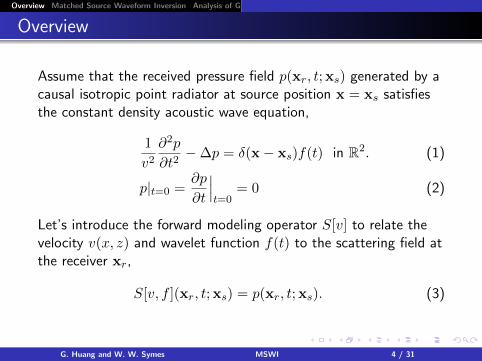
Assume that the received pressure field p(xr, t;xs) generated by acausal isotropic point radiator at source position x = xs satisfiesthe constant density acoustic wave equation,
1
v2∂2p
∂t2−∆p = δ(x− xs)f(t) in R2. (1)
p|t=0 =∂p
∂t
∣∣∣t=0
= 0 (2)
Let’s introduce the forward modeling operator S[v] to relate thevelocity v(x, z) and wavelet function f(t) to the scattering field atthe receiver xr,
S[v, f ](xr, t;xs) = p(xr, t;xs). (3)
G. Huang and W. W. Symes MSWI 4 / 31
Overview Matched Source Waveform Inversion Analysis of Gradient and Hessian Numerical Examples Conclusion and Discussion
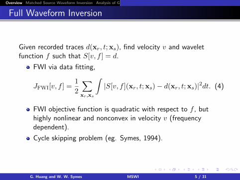
Full Waveform Inversion
Given recorded traces d(xr, t;xs), find velocity v and waveletfunction f such that S[v, f ] = d.
FWI via data fitting,
JFWI[v, f ] =1
2
∑xr,xs
∫|S[v, f ](xr, t;xs)− d(xr, t;xs)|2dt. (4)
FWI objective function is quadratic with respect to f , buthighly nonlinear and nonconvex in velocity v (frequencydependent).
Cycle skipping problem (eg. Symes, 1994).
G. Huang and W. W. Symes MSWI 5 / 31
Overview Matched Source Waveform Inversion Analysis of Gradient and Hessian Numerical Examples Conclusion and Discussion
Outline
1 Overview
2 Matched Source Waveform Inversion
3 Analysis of Gradient and Hessian
4 Numerical Examples
5 Conclusion and Discussion
G. Huang and W. W. Symes MSWI 6 / 31
Overview Matched Source Waveform Inversion Analysis of Gradient and Hessian Numerical Examples Conclusion and Discussion
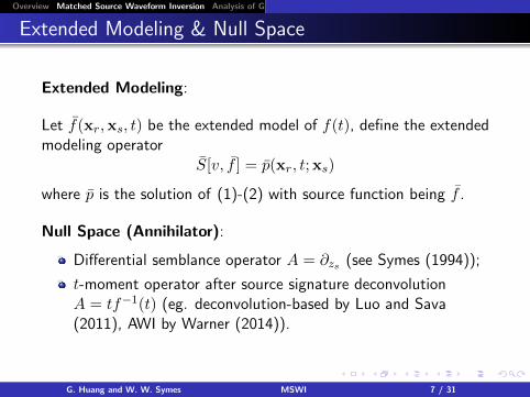
Extended Modeling & Null Space
Extended Modeling:
Let f̄(xr,xs, t) be the extended model of f(t), define the extendedmodeling operator
S̄[v, f̄ ] = p̄(xr, t;xs)
where p̄ is the solution of (1)-(2) with source function being f̄ .
Null Space (Annihilator):
Differential semblance operator A = ∂zs (see Symes (1994));
t-moment operator after source signature deconvolutionA = tf−1(t) (eg. deconvolution-based by Luo and Sava(2011), AWI by Warner (2014)).
G. Huang and W. W. Symes MSWI 7 / 31
Overview Matched Source Waveform Inversion Analysis of Gradient and Hessian Numerical Examples Conclusion and Discussion
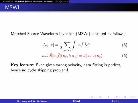
MSWI
Matched Source Waveform Inversion (MSWI) is stated as follows,
JMS[v] =1
2
∑xr,xs
∫|Af̄ |2dt (5)
s.t. S̄[v, f̄ ](xr, t;xs) = d(xr, t;xs). (6)
Key feature: Even given wrong velocity, data fitting is perfect,hence no cycle skipping problem!
G. Huang and W. W. Symes MSWI 8 / 31
Overview Matched Source Waveform Inversion Analysis of Gradient and Hessian Numerical Examples Conclusion and DiscussionAnalysis of Gradient Local Convexity of Hessian Relation with DSO formulation
Outline
1 Overview
2 Matched Source Waveform Inversion
3 Analysis of Gradient and HessianAnalysis of GradientLocal Convexity of HessianRelation with DSO formulation
4 Numerical Examples
5 Conclusion and Discussion
G. Huang and W. W. Symes MSWI 9 / 31
Overview Matched Source Waveform Inversion Analysis of Gradient and Hessian Numerical Examples Conclusion and DiscussionAnalysis of Gradient Local Convexity of Hessian Relation with DSO formulation
1 Overview
2 Matched Source Waveform Inversion
3 Analysis of Gradient and HessianAnalysis of GradientLocal Convexity of HessianRelation with DSO formulation
4 Numerical Examples
5 Conclusion and Discussion
G. Huang and W. W. Symes MSWI 10 / 31
Overview Matched Source Waveform Inversion Analysis of Gradient and Hessian Numerical Examples Conclusion and DiscussionAnalysis of Gradient Local Convexity of Hessian Relation with DSO formulation
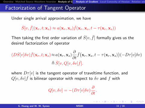
Factorization of Tangent Operator
Under single arrival approximation, we have
S̄[v, f̄ ](xr, t;xs) ≈ a(xr,xs)f̄(xr,xs, t− τ(xr,xs))
Then taking the first order variation of S̄[v, f̄ ] formally gives us thedesired factorization of operator
(DS̄[v]δv)f̄(xr, t;xs)≈a(xr,xs)∂
∂tf̄(xr,xs, t− τ(xr,xs)
)(−Dτ [v]δv)
, S̄[v,Q[v, δv]f̄ ].
where Dτ [v] is the tangent operator of traveltime function, andQ[v, δv]f̄ is bilinear operator with respect to δv and f with
Q[v, δv] = −(Dτ [v]δv)∂
∂t.
G. Huang and W. W. Symes MSWI 11 / 31
Overview Matched Source Waveform Inversion Analysis of Gradient and Hessian Numerical Examples Conclusion and DiscussionAnalysis of Gradient Local Convexity of Hessian Relation with DSO formulation
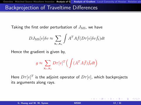
Backprojection of Traveltime Differences
Taking the first order perturbation of JMS, we have
DJMS[v]δv ≈∑xr,xs
∫ATAf̄(Dτ [v]δvf̄t)dt
Hence the gradient is given by,
g ≈∑xr,xs
Dτ [v]T(∫
(ATAf̄)f̄tdt)
Here Dτ [v]T is the adjoint operator of Dτ [v], which backprojectsits arguments along rays.
G. Huang and W. W. Symes MSWI 12 / 31
Overview Matched Source Waveform Inversion Analysis of Gradient and Hessian Numerical Examples Conclusion and DiscussionAnalysis of Gradient Local Convexity of Hessian Relation with DSO formulation
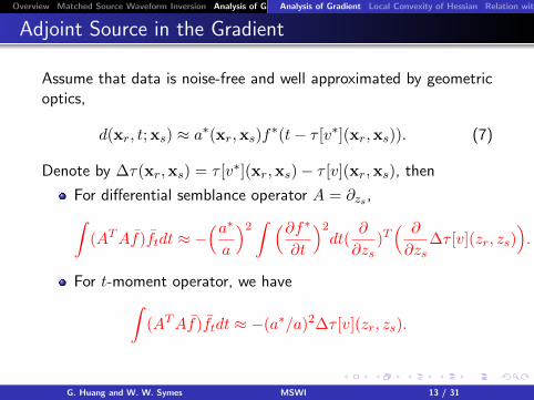
Adjoint Source in the Gradient
Assume that data is noise-free and well approximated by geometricoptics,
d(xr, t;xs) ≈ a∗(xr,xs)f∗(t− τ [v∗](xr,xs)). (7)
Denote by ∆τ(xr,xs) = τ [v∗](xr,xs)− τ [v](xr,xs), then
For differential semblance operator A = ∂zs ,∫(ATAf̄)f̄tdt ≈ −
(a∗a
)2 ∫ (∂f∗∂t
)2dt(
∂
∂zs)T( ∂
∂zs∆τ [v](zr, zs)
).
For t-moment operator, we have∫(ATAf̄)f̄tdt ≈ −(a∗/a)2∆τ [v](zr, zs).
G. Huang and W. W. Symes MSWI 13 / 31
Overview Matched Source Waveform Inversion Analysis of Gradient and Hessian Numerical Examples Conclusion and DiscussionAnalysis of Gradient Local Convexity of Hessian Relation with DSO formulation
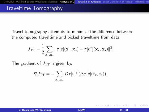
Traveltime Tomography
Travel tomography attempts to minimize the difference betweenthe computed traveltime and picked traveltime from data,
JTT =1
2
∑xr,xs
‖τ [v](xr,xs)− τ [v∗](xr,xs)‖2,
The gradient of JTT is given by,
∇JTT = −∑xr,xs
Dτ [v]T (∆τ [v](zr, zs)).
G. Huang and W. W. Symes MSWI 14 / 31
Overview Matched Source Waveform Inversion Analysis of Gradient and Hessian Numerical Examples Conclusion and DiscussionAnalysis of Gradient Local Convexity of Hessian Relation with DSO formulation
1 Overview
2 Matched Source Waveform Inversion
3 Analysis of Gradient and HessianAnalysis of GradientLocal Convexity of HessianRelation with DSO formulation
4 Numerical Examples
5 Conclusion and Discussion
G. Huang and W. W. Symes MSWI 15 / 31
Overview Matched Source Waveform Inversion Analysis of Gradient and Hessian Numerical Examples Conclusion and DiscussionAnalysis of Gradient Local Convexity of Hessian Relation with DSO formulation
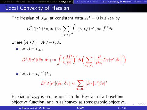
Local Convexity of Hessian
The Hessian of JMS at consistent data Af̄ = 0 is given by
D2J [v∗](δv, δv) ≈∑xr,xs
∫|[A,Q](v∗, δv)f̄ |2dt
where [A,Q] = AQ−QA.
for A = ∂zs ,
D2J [v∗](δv, δv) ≈∫ (∂f∗
∂t
)2dt( ∑
xr,xs
∣∣∣ ∂∂zs
Dτ [v∗]δv∣∣∣2)
for A = tf−1(t),
D2J [v∗](δv, δv) ≈∑xr,xs
|Dτ [v∗]δv|2
Hessian of JMS is proportional to the Hessian of a traveltimeobjective function, and is as convex as tomographic objective.
G. Huang and W. W. Symes MSWI 16 / 31
Overview Matched Source Waveform Inversion Analysis of Gradient and Hessian Numerical Examples Conclusion and DiscussionAnalysis of Gradient Local Convexity of Hessian Relation with DSO formulation
1 Overview
2 Matched Source Waveform Inversion
3 Analysis of Gradient and HessianAnalysis of GradientLocal Convexity of HessianRelation with DSO formulation
4 Numerical Examples
5 Conclusion and Discussion
G. Huang and W. W. Symes MSWI 17 / 31
Overview Matched Source Waveform Inversion Analysis of Gradient and Hessian Numerical Examples Conclusion and DiscussionAnalysis of Gradient Local Convexity of Hessian Relation with DSO formulation
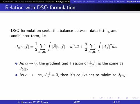
Relation with DSO formulation
DSO formulation seeks the balance between data fitting andannihilator term, i.e.
Jα[v, f̄ ] =1
2
∑xr,xs
∫|S̄[v, f̄ ]− d|2dt+
α
2
∑xr,xs
∫|Af̄ |2dt.
As α→ 0, the gradient and Hessian of 1αJα is the same as
JMS.
As α→ +∞, Af̄ = 0, then it’s equivalent to minimize JFWI
G. Huang and W. W. Symes MSWI 18 / 31
Overview Matched Source Waveform Inversion Analysis of Gradient and Hessian Numerical Examples Conclusion and Discussion
Outline
1 Overview
2 Matched Source Waveform Inversion
3 Analysis of Gradient and Hessian
4 Numerical Examples
5 Conclusion and Discussion
G. Huang and W. W. Symes MSWI 19 / 31
Overview Matched Source Waveform Inversion Analysis of Gradient and Hessian Numerical Examples Conclusion and Discussion
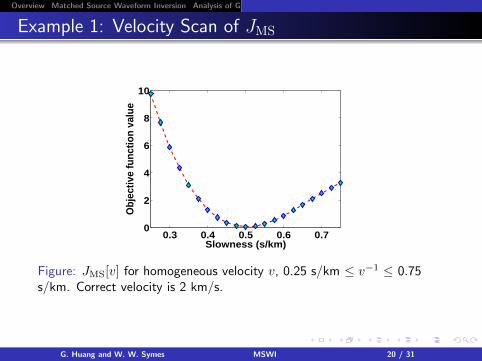
Example 1: Velocity Scan of JMS
0.3 0.4 0.5 0.6 0.70
2
4
6
8
10
Slowness (s/km)
Obj
ectiv
e fu
nctio
n va
lue
Figure: JMS[v] for homogeneous velocity v, 0.25 s/km ≤ v−1 ≤ 0.75s/km. Correct velocity is 2 km/s.
G. Huang and W. W. Symes MSWI 20 / 31
Overview Matched Source Waveform Inversion Analysis of Gradient and Hessian Numerical Examples Conclusion and Discussion
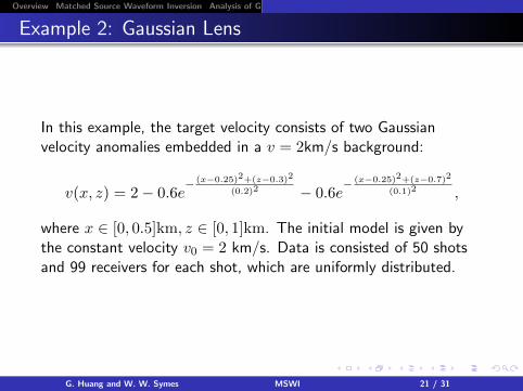
Example 2: Gaussian Lens
In this example, the target velocity consists of two Gaussianvelocity anomalies embedded in a v = 2km/s background:
v(x, z) = 2− 0.6e− (x−0.25)2+(z−0.3)2
(0.2)2 − 0.6e− (x−0.25)2+(z−0.7)2
(0.1)2 ,
where x ∈ [0, 0.5]km, z ∈ [0, 1]km. The initial model is given bythe constant velocity v0 = 2 km/s. Data is consisted of 50 shotsand 99 receivers for each shot, which are uniformly distributed.
G. Huang and W. W. Symes MSWI 21 / 31
Overview Matched Source Waveform Inversion Analysis of Gradient and Hessian Numerical Examples Conclusion and Discussion
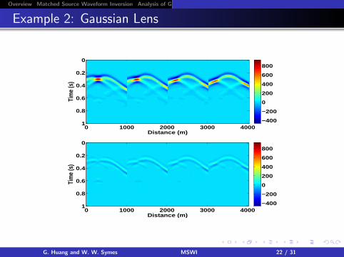
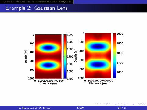
Example 2: Gaussian Lens
Distance (m)
Tim
e (s
)
0 1000 2000 3000 4000
0
0.2
0.4
0.6
0.8
1 −400
−200
0
200
400
600
800
Distance (m)
Tim
e (s
)
0 1000 2000 3000 4000
0
0.2
0.4
0.6
0.8
1 −400
−200
0
200
400
600
800
G. Huang and W. W. Symes MSWI 22 / 31
Overview Matched Source Waveform Inversion Analysis of Gradient and Hessian Numerical Examples Conclusion and Discussion
Example 2: Gaussian Lens
Distance (m)
Dep
th (
m)
0 100 200 300 400 500
0
200
400
600
800
1000 1400
1500
1600
1700
1800
1900
2000
Distance (m)
Dep
th (
m)
0 100200300400500
0
200
400
600
800
1000
1600
1700
1800
1900
2000
G. Huang and W. W. Symes MSWI 23 / 31
Overview Matched Source Waveform Inversion Analysis of Gradient and Hessian Numerical Examples Conclusion and Discussion
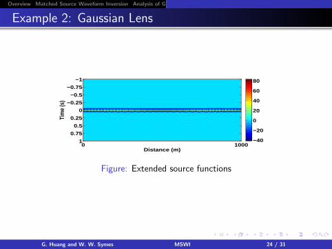
Example 2: Gaussian Lens
Distance (m)
Tim
e (s
)
0 1000
−1
−0.75
−0.5
−0.25
0
0.25
0.5
0.75
1 −40
−20
0
20
40
60
80
Figure: Extended source functions
G. Huang and W. W. Symes MSWI 24 / 31
Overview Matched Source Waveform Inversion Analysis of Gradient and Hessian Numerical Examples Conclusion and Discussion
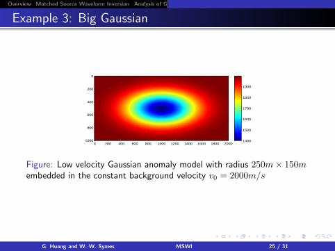
Example 3: Big Gaussian
0 200 400 600 800 1000 1200 1400 1600 1800 2000
0
200
400
600
800
1000 1400
1500
1600
1700
1800
1900
Figure: Low velocity Gaussian anomaly model with radius 250m× 150membedded in the constant background velocity v0 = 2000m/s
G. Huang and W. W. Symes MSWI 25 / 31
Overview Matched Source Waveform Inversion Analysis of Gradient and Hessian Numerical Examples Conclusion and Discussion
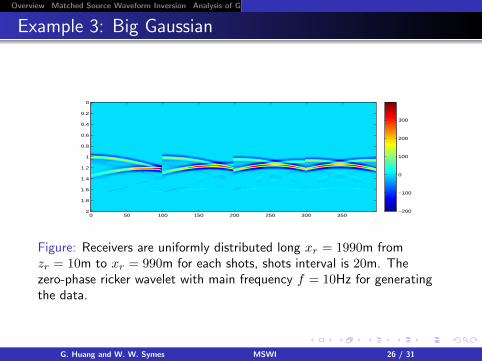
Example 3: Big Gaussian
0 50 100 150 200 250 300 350
0
0.2
0.4
0.6
0.8
1
1.2
1.4
1.6
1.8
2 −200
−100
0
100
200
300
Figure: Receivers are uniformly distributed long xr = 1990m fromzr = 10m to xr = 990m for each shots, shots interval is 20m. Thezero-phase ricker wavelet with main frequency f = 10Hz for generatingthe data.
G. Huang and W. W. Symes MSWI 26 / 31
Overview Matched Source Waveform Inversion Analysis of Gradient and Hessian Numerical Examples Conclusion and Discussion
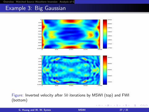
Example 3: Big Gaussian
0 500 1000 1500 2000
0
100
200
300
400
500
600
700
800
900
1000 1700
1750
1800
1850
1900
1950
2000
2050
0 500 1000 1500 2000
0
100
200
300
400
500
600
700
800
900
1000
1500
2000
2500
3000
3500
Figure: Inverted velocity after 50 iterations by MSWI (top) and FWI(bottom)
G. Huang and W. W. Symes MSWI 27 / 31
Overview Matched Source Waveform Inversion Analysis of Gradient and Hessian Numerical Examples Conclusion and Discussion
Outline
1 Overview
2 Matched Source Waveform Inversion
3 Analysis of Gradient and Hessian
4 Numerical Examples
5 Conclusion and Discussion
G. Huang and W. W. Symes MSWI 28 / 31
Overview Matched Source Waveform Inversion Analysis of Gradient and Hessian Numerical Examples Conclusion and Discussion
Conclusion and Discussion
Conclusion
Establish the relation between waveform inversion andtraveltime tomography;
Convexity of objective function is independent of frequencycontent.
MSWI still get stuck in local minima due to the strongmultipaths.
Discussion
Does perfect data fitting (no cycle skipping) mean avoidinglocal minima;
How do we choose the extended model space and the relatedannihilator.
G. Huang and W. W. Symes MSWI 29 / 31
Overview Matched Source Waveform Inversion Analysis of Gradient and Hessian Numerical Examples Conclusion and Discussion
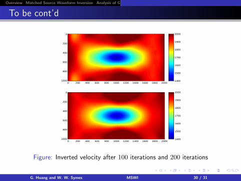
To be cont’d
0 200 400 600 800 1000 1200 1400 1600 1800 2000
0
200
400
600
800
1000 1400
1500
1600
1700
1800
1900
2000
0 200 400 600 800 1000 1200 1400 1600 1800 2000
0
200
400
600
800
1000 1400
1500
1600
1700
1800
1900
2000
Figure: Inverted velocity after 100 iterations and 200 iterations
G. Huang and W. W. Symes MSWI 30 / 31
Overview Matched Source Waveform Inversion Analysis of Gradient and Hessian Numerical Examples Conclusion and Discussion
Thanks
Total E&P USA, for funding me
The Rice Inversion Project, for supporting me
TRIP members, for helping me
All of you, for listening to me
G. Huang and W. W. Symes MSWI 31 / 31