Wave-equation Reflection Traveltime InversionSanzong Zhang∗, Gerard Schuster, King Abdullah University of Science and Technology,and Yi Luo, Saudi Aramco

SUMMARY

The main difficulty with iterative waveform inversion using agradient optimization method is that it tends to get stuck inlocal minima associated within the waveform misfit function.This is because the waveform misfit function is highly non-linear with respect to changes in the velocity model. To reducethis nonlinearity, we present a reflection traveltime tomogra-phy method based on the wave equation which enjoys a morequasi-linear relationship between the model and the data. Alocal crosscorrelation of the windowed downgoing direct waveand the upgoing reflection wave at the image point yields thelag time that maximizes the correlation. This lag time repre-sents the reflection traveltime residual that is back-projectedinto the earth model to update the velocity in the same way aswave-equation transmission traveltime inversion. No travel-time picking is needed and no high-frequency approximationis assumed. The mathematical derivation and the numericalexamples are presented to partly demonstrate its efficiency androbustness.

INTRODUCTION

Prestack depth migration of 3D seismic data is the industrystandard for computing detailed estimates of the earth’s re-flectivity distribution. However, an accurate velocity modelis a precondition for imaging complex geological structures.To estimate this velocity model, there are three primary inver-sion methods: migration velocity analysis (MVA), traveltimeinversion, and full waveform inversion. For migration veloc-ity analysis (Symes and Kern, 1994; Sava and Biondi, 2004;Shen and Calandra, 2005), the optimal migration velocity isthe one that best flattens the reflection events in a common im-age gather. For traveltime inversion (Dines and Lytle, 1979;Paulsson et al., 1985; Ivansson, 1985; Bishop et al., 1985;Lines, 1988), the traveltimes of refraction and reflection ar-rivals are used to invert for smooth features of the velocitymodel, while full waveform inversion (Tarantola, 1986, 1987;Mora, 1987; Crase et al., 1992; Zhou et al., 1995; Pratt, 1998)inverts the waveform information for fine details of the earthmodel.A more detailed analysis shows that traveltime inversion isconstrained by a high-frequency approximation, and so it failsto invert for the earth’s velocity variations having nearly thesame wavelength or less than that of the source wavelet. Con-sequently, the resolution of the velocity model constructed fromthe traveltimes is much less than that of full waveform inver-sion. The merit is that the traveltime misfit function (normedsquared error between observed and calculated traveltimes) isquasi-linear with respect to velocity perturbations so that anefficient velocity inversion can be achieved even if the start-ing model is far from the actual model (Luo and Schuster,

1991a and 1991b; Zhou et al., 1995). Although very sen-sitive to the choice of starting models or noisy amplitudes,full waveform inversion can sometimes reconstruct a finely de-tailed estimation of the earth model. This is because there is nohigh-frequency assumption about the data, and almost all seis-mic events are embedded in the misfit function. The problemwith full waveform inversion, however, is that its misfit func-tion (normed squared error between the observed and syntheticseismograms) can be highly nonlinear with respect to changesin the velocity model. In this case, a gradient method will tendto get stuck in a local minima if the starting model is far awayfrom the actual model.

To exploit the strengths and ameliorate the weaknesses of bothray-based traveltime tomography and full waveform inversion,wave-equation-based traveltime inversion was developed to in-vert the velocity model (Luo and Schuster, 1991a and 1991b;Zhou et al, 1995; Zhang and Wang, 2009; Leeuwen and Mul-der, 2010). This kind of inversion methods inverts traveltimeusing the gradient calculated from the wave equation. It isnot constrained by a high-frequency approximation and trav-eltime picking is not necessary. Other important benefits area convergence rate that is somewhat insensitive to the startingmodel, a high degree of model resolution, and a robustness inthe presence of data noise. However, these traveltime inversionmethods are designed to invert transmission waves in seismicdata, and are not designed to invert the reflection traveltimes.Unlike refraction and direct waves, reflection waves can pro-vide more velocity information about the deeper subsurface formodel inversion. However, full waveform inversion of reflec-tion wave is difficult if the initial velocity model is far from thetrue model. To overcome this limitation, this paper presents theextension of wave-equation transmission traveltime inversion(WTI) (Luo and Schuster, 1991a and 1991b) to wave-equationreflection traveltime inversion (WRTI).

This paper is organized into three sections. The first sectiondescribes the basic theory of image-domain wave-equation re-flection traveltime inversion. The second section shows nu-merical examples to verify the effectiveness of this method.The last section draws some conclusions.

THEORY

The key step in WRTI is to transform the reflection data intothat recorded by a virtual transmission experiment. This trans-mission data can then be inverted by WTI (Luo and Schus-ter,1991a).1). Assume an initial velocity model.2). Migrate the recorded upgoing reflection data to get the im-age points atx.3). Forward propagate the source atxs to x to get the downgo-ing direct waveps(x,t) as shown in Figure 1(a). Now we havethe virtual source waveletps(x,t) where the virtual source is

© 2011 SEGSEG San Antonio 2011 Annual Meeting 27052705

Wave-equation Reflection Traveltime Inversion

at x, which will be used to update the velocity on the receiverside.4). Backpropagate the observed reflection data fromxg to theimage pointx and get the upgoing reflection wavepg(x,t) asshown in Figure 1(b). Now we have the virtual reflection dataat x which can be used to find the the traveltime differencebetween the downgoing direct waveps(x,t) and the upgoingreflection wavepg(x,t).5). Crosscorrelate the downgoing direct event inps(x,t) andthe upgoing reflection event inpg(x,t) to find the time shift∆τbetween them as shown in Figure 1(c).6). Update the velocity model by smearing∆τ along the weightedwavepath betweenxs andx and betweenx andxg as shown inFigure 1(d). This step is actually the application of WTI to thevirtual transmission data.7). Repeat steps (3)-(6) for all source and image points.8). Go back to step (2) until the norm of the traveltime residualsatisfies the specified minimum.In summary, WRTI can be decomposed into two steps. Thefirst step is to redatum the geophones from the free surface tothe image points. The second step is to redatum the source tothe image point. Hence, two virtual transmission experimentsare formed and used to update the velocity model. The po-tential benefit is that reflection traveltime inversion might en-joy robust convergence properties and not require the tediouspicking of reflection traveltimes.

s

x

g

ps(x,t) pg(x,t)

!

!

(a) Forward extrapolate source

(b) Backward extrapolate geophones

(c) Crosscorrelate

s g

x

s g

x ps(x,t)

s g

x

(d) Searing along wavepath

s

x

g

pg(x,t)

Figure 1: (a). The forward extrapolation of the source field.(b). The backward extrapolation of the geophone field. (c).The crosscorrelation of the downgoing direct wave and the up-going reflection wave. (d). The misfit gradient is propertial tothe ∆τ weighted wavepath functions between the source andthe image points, and the image point and the geophones.

Connective functionThe following analysis assumes that the propagation of seismicwaves honors the 2-D acoustic wave equation. Letp(xr,t|xs)obsbe the pressure at timet observed at the receiver locationxr

due to a source atxs. The source is always assumed to be ini-tiated at zero time. For a given velocity model,p(xr,t|xs)caldenotes the calculated seismogram that honors the 2D acous-tic wave equation. The crosscorrelation function between the

forward wavefield and the backward wavefield can be used todetermine the image atx

f (x,τ) =

∫

dt ps(x,t + τ)pg(x,t), (1)

where ps(x,t + τ) is the forward wavefield initiated by thesource atxs

ps(x,t) = p(x,t|xs)cal = w(t)∗g(x,t|xs,0). (2)

Herew(t) is the source wavelet, andg(x,t|xs,0) is the Green’sfunction. pg(x,t) is the backward wavefield by the time-reversedpropagation of the observed datap(xg,t|xs)obs

pg(x,t) =

∫

p(xg,t|xs)obs ∗g(x,−t|xg,0)dxg, (3)

andτ is the time lag of the crosscorrelation function. Whenτ = 0, equation (2) is the conventional correlation imagingcondition. The nonzero time lag indicates the inaccuracy ofthe velocity model. The extremum off (x,τ) should satisfy

f (x,∆τ) = max{ f (x,τ)|τ ∈ [−T,T ]} (4)

or

f (x,∆τ) = min{ f (x,τ)|τ ∈ [−T,T ]}, (5)

whereT is the estimated maximum time lag between the for-ward modeled wave from the source and the backward prop-agated wave from the receivers. Note∆τ = 0 indicates thatthe correct velocity model has been found which generates adowngoing direct wave and upgoing reflection wave arrivingat the same time. The derivative off (x,τ) with respect toτshould be zero at∆τ unless its maximum or minimum is at anend pointT or −T :

f∆τ =∂ f (x,τ)

∂τ|τ=∆τ =

∫

dt ps(x,t + τ)pg(x,t) = 0, (6)

where ps(x,t + τ) represents the time derivative of the calcu-lated downgoing wave.

Misfit functionThe inverse problem is defined as finding a velocity model thatminimizes the following misfit function:

S =12

∑

s

∑

x

(∆τ)2. (7)

Herex is the image point, ands is the source position. The re-flection traveltime inversion is computed by findingc(x′) thatminimizing the sum of the squared traveltime residuals. Forsimplicity, a steepest descent non-linear optimization methodis used to describe the iterative minimization of equation (7),with the understanding that a preconditioned conjugate gradi-ent method is used in practice. To update the velocity model,the steepest descent method gives

ck+1(x′) = ck(x

′)+αk · γk(x′), (8)

© 2011 SEGSEG San Antonio 2011 Annual Meeting 27062706

Wave-equation Reflection Traveltime Inversion

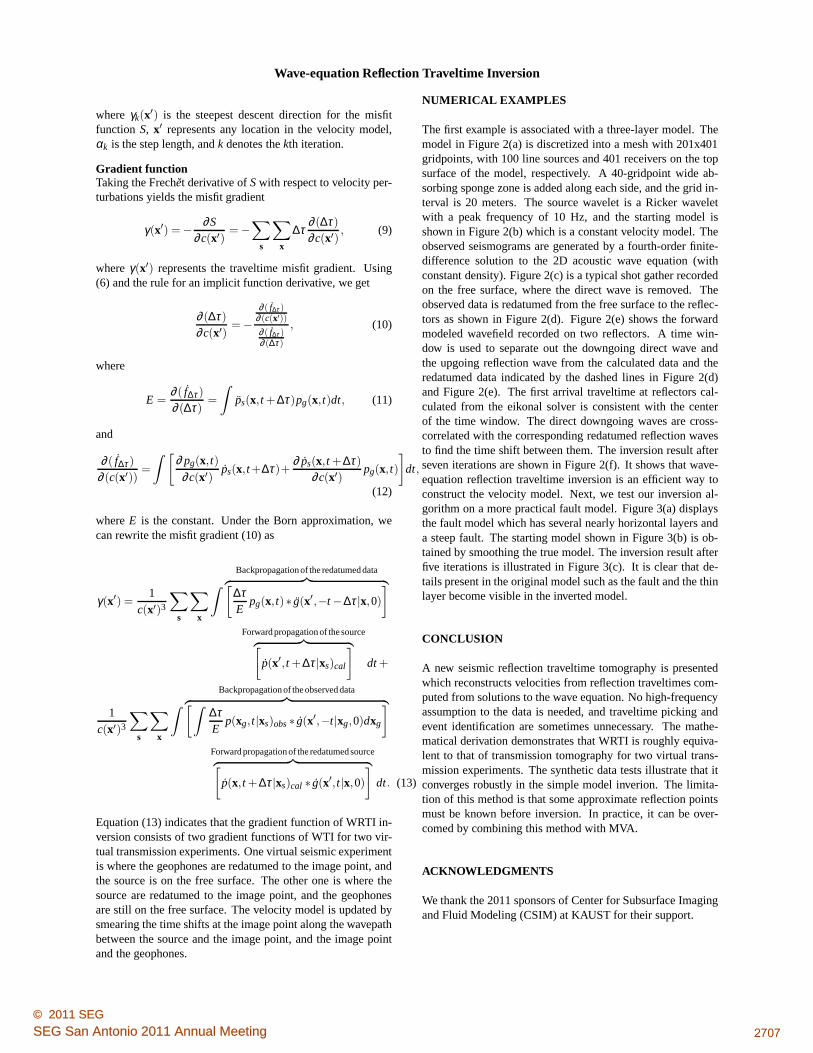
where γk(x′) is the steepest descent direction for the misfitfunction S, x′ represents any location in the velocity model,αk is the step length, andk denotes thekth iteration.

Gradient functionTaking the Frech˘et derivative ofS with respect to velocity per-turbations yields the misfit gradient

γ(x′) = −∂S

∂c(x′)= −

∑

s

∑

x

∆τ∂ (∆τ)

∂c(x′), (9)

whereγ(x′) represents the traveltime misfit gradient. Using(6) and the rule for an implicit function derivative, we get

∂ (∆τ)

∂c(x′)= −

∂ ( f∆τ )∂ (c(x′))

∂ ( f∆τ )∂ (∆τ)

, (10)

where

E =∂ ( f∆τ)

∂ (∆τ)=

∫

ps(x,t +∆τ)pg(x,t)dt, (11)

and

∂ ( f∆τ)

∂ (c(x′))=

∫ [∂ pg(x,t)

∂c(x′)ps(x,t +∆τ)+

∂ ps(x,t +∆τ)

∂c(x′)pg(x,t)

]

dt,

(12)

whereE is the constant. Under the Born approximation, wecan rewrite the misfit gradient (10) as

γ(x′) =1

c(x′)3

∑

s

∑

x

∫

Backpropagationof the redatumeddata︷ ︸︸ ︷[

∆τE

pg(x,t)∗ g(x′,−t −∆τ|x,0)

]

Forwardpropagationof the source︷ ︸︸ ︷[

p(x′,t +∆τ|xs)cal

]

dt +

1c(x′)3

∑

s

∑

x

∫

Backpropagationof the observeddata︷ ︸︸ ︷[∫

∆τE

p(xg,t|xs)obs ∗ g(x′,−t|xg,0)dxg

]

Forwardpropagationof the redatumedsource︷ ︸︸ ︷[

p(x,t +∆τ|xs)cal ∗ g(x′,t|x,0)

]

dt. (13)

Equation (13) indicates that the gradient function of WRTI in-version consists of two gradient functions of WTI for two vir-tual transmission experiments. One virtual seismic experimentis where the geophones are redatumed to the image point, andthe source is on the free surface. The other one is where thesource are redatumed to the image point, and the geophonesare still on the free surface. The velocity model is updated bysmearing the time shifts at the image point along the wavepathbetween the source and the image point, and the image pointand the geophones.

NUMERICAL EXAMPLES

The first example is associated with a three-layer model. Themodel in Figure 2(a) is discretized into a mesh with 201x401gridpoints, with 100 line sources and 401 receivers on the topsurface of the model, respectively. A 40-gridpoint wide ab-sorbing sponge zone is added along each side, and the grid in-terval is 20 meters. The source wavelet is a Ricker waveletwith a peak frequency of 10 Hz, and the starting model isshown in Figure 2(b) which is a constant velocity model. Theobserved seismograms are generated by a fourth-order finite-difference solution to the 2D acoustic wave equation (withconstant density). Figure 2(c) is a typical shot gather recordedon the free surface, where the direct wave is removed. Theobserved data is redatumed from the free surface to the reflec-tors as shown in Figure 2(d). Figure 2(e) shows the forwardmodeled wavefield recorded on two reflectors. A time win-dow is used to separate out the downgoing direct wave andthe upgoing reflection wave from the calculated data and theredatumed data indicated by the dashed lines in Figure 2(d)and Figure 2(e). The first arrival traveltime at reflectors cal-culated from the eikonal solver is consistent with the centerof the time window. The direct downgoing waves are cross-correlated with the corresponding redatumed reflection wavesto find the time shift between them. The inversion result afterseven iterations are shown in Figure 2(f). It shows that wave-equation reflection traveltime inversion is an efficient way toconstruct the velocity model. Next, we test our inversion al-gorithm on a more practical fault model. Figure 3(a) displaysthe fault model which has several nearly horizontal layers anda steep fault. The starting model shown in Figure 3(b) is ob-tained by smoothing the true model. The inversion result afterfive iterations is illustrated in Figure 3(c). It is clear that de-tails present in the original model such as the fault and the thinlayer become visible in the inverted model.

CONCLUSION

A new seismic reflection traveltime tomography is presentedwhich reconstructs velocities from reflection traveltimes com-puted from solutions to the wave equation. No high-frequencyassumption to the data is needed, and traveltime picking andevent identification are sometimes unnecessary. The mathe-matical derivation demonstrates that WRTI is roughly equiva-lent to that of transmission tomography for two virtual trans-mission experiments. The synthetic data tests illustrate that itconverges robustly in the simple model inverion. The limita-tion of this method is that some approximate reflection pointsmust be known before inversion. In practice, it can be over-comed by combining this method with MVA.

ACKNOWLEDGMENTS

We thank the 2011 sponsors of Center for Subsurface Imagingand Fluid Modeling (CSIM) at KAUST for their support.

© 2011 SEGSEG San Antonio 2011 Annual Meeting 27072707

Wave-equation Reflection Traveltime Inversion

x (km)

z (k

m)

True Model

0 1 2 3 4 5 6 7 8

0

1

2

3

4 2500

2600

2700

2800

2900

3000

(a)

x (km)

z (k

m)

Initial Model

0 1 2 3 4 5 6 7 8

0

1

2

3

4 2500

2600

2700

2800

2900

3000

(b)

CSG

x (km)

t (s)

0 1 2 3 4 5 6 7 8

0

1

2

3

4

(c)

Redatumed Upcoming Wave

Reflection point

t (s)

0 100 200 300 400 500 600 700 800

0

1

2

3

4

(d)

Calculated Downgoign Wave

Reflection point

t (s)

0 100 200 300 400 500 600 700 800

0

1

2

3

4

(e)

x (km)

z (k

m)

Inversion Result

0 1 2 3 4 5 6 7 8

0

1

2

3

4 2500

2600

2700

2800

2900

3000

(f)

Figure2: (a). Three-layer true velocity model. (b). The initial constant velocity model. (c). The observed data. The direct waveis removed. (d). The upgoing reflection wave which is obtained by redatuming the observed data from the free surface to thereflectors. (e). The calculated downgoing wave on the reflectors. (f). The inversion result after seven iterations.

x (km)

z (k

m)

True Model

0 5 10 15

0

1

2

3

4

5

6

74000

6000

8000

10000

12000

(a)

x (km)

z (k

m)

Initial Model

0 5 10 15

0

1

2

3

4

5

6

74000

6000

8000

10000

12000

(b)

x (km)

z (k

m)

Inversion Result

0 5 10 15

0

1

2

3

4

5

6

74000

6000

8000

10000

12000

(c)

Figure3: (a). The true velocity model with a fault. (b). The initial velocity model. (c). The inversion result after ten iterations.

© 2011 SEGSEG San Antonio 2011 Annual Meeting 27082708

EDITED REFERENCES

Note: This reference list is a copy-edited version of the reference list submitted by the author. Reference lists for the 2011

SEG Technical Program Expanded Abstracts have been copy edited so that references provided with the online metadata for

each paper will achieve a high degree of linking to cited sources that appear on the Web.

REFERENCES

Bishop, T., K. Bube, R. Cutler, R. Langan, P. Love, J. Resnick, R. Shuey, D. Spindler, and H. Wyld,

1985, Tomographic determination of velocity and depth in laterally varying media: Geophysics, 50,

903–923, doi:10.1190/1.1441970.

Crase, E., C. Wideman, M. Noble, and A. Tarantola, 1992, Nonlinear elastic waveform inversion of land

seismic reflection data: Journal of Geophysics Research, 97, 4685–4704.

Dines, K., and R. Lytle, 1979, Computerized geophysical tomography: Proceedings of the IEEE, 67,

1065–1073, doi:10.1109/PROC.1979.11390.

Ivansson, S., 1985, A study of methods for tomographic velocity estimation in the presence of low-

velocity zones: Geophysics, 50, 969–988, doi:10.1190/1.1441975.

Levander, A. R., 1988, Fourth-order finite-difference P-SV seismograms: Geophysics, 53, 1425–1436,

doi:10.1190/1.1442422.

Lines, L., 1988, Inversion of geophysical data: SEG Geophysics Reprint Series No. 9.

Luo, Y., and G. Schuster, 1991a, Wave equation traveltime inversion: Geophysics, 56, 645–653,

doi:10.1190/1.1443081.

Luo, Y., and G. Schuster, 1991b, Wave equation inversion of skeletonized geophysical data: Geophysical

Journal International, 105, 289–294, doi:10.1111/j.1365-246X.1991.tb06713.x.

Mora, P., 1987, Nonlinear two-dimensional elastic inversion of multioffset seismic data: Geophysics, 52,

1211–1228, doi:10.1190/1.1442384.

Paulsson, B., N. Cook, and T. McEvilly, 1985, Elastic wave velocities and attenuation in an underground

granitic repository for nuclear waste: Geophysics, 50, 551–570, doi:10.1190/1.1441932.

Pratt, R. G., C. Shin, and G. J. Hicks, 1998, Gauss-Newton and full Newton methods in frequency-space

seismic waveform inversion: Geophysical Journal International, 133, 341–362, doi:10.1046/j.1365-

246X.1998.00498.x.

Sava, P., and B. Biondi, 2004, Wave-equation migration velocity analysis, I: Theory: Geophysical

Prospecting, 52, 593–606.

Shen, P., and H. Calandra, 2005, One-way waveform inversion within the framework of adjoint state

differential migration: 75th Annual International Meeting, SEG, Expanded Abstracts, 1709–1712.

Symes, W., and M. Kern, 1994, Inversion of reflection seismograms by differential semblance analysis:

Algorithm structure and synthetic examples: Geophysical Prospecting, 42, 565–614,

doi:10.1111/j.1365-2478.1994.tb00231.x.

Tarantola, A., 1986, A strategy for nonlinear elastic inversion of seismic reflection data: Geophysics, 51,

1893–1903, doi:10.1190/1.1442046.

Tarantola, A., 1987, Inverse problem theory: Elsevier.

© 2011 SEGSEG San Antonio 2011 Annual Meeting 27092709

van Leeuwen, T., and W. A. Mulder, 2010, A correlation-based misfit criterion for wave-equation

traveltime tomography: Geophysical Journal International, 182, 1383–1394, doi:10.1111/j.1365-

246X.2010.04681.x.

Zhou, C., W. Cai, Y. Luo, G. Schuster, and S. Hassanzadeh, 1995, Acoustic wave-equation traveltime and

waveform inversion of crosshole seismic data: Geophysics, 60, 765–773, doi:10.1190/1.1443815.

© 2011 SEGSEG San Antonio 2011 Annual Meeting 27102710