water distribution system failures: an integrated framework for prognostic and diagnostic analyses

WATER DISTRIBUTION SYSTEM FAILURES: AN INTEGRATED FRAMEWORK

FOR PROGNOSTIC AND DIAGNOSTIC ANALYSIS

by

Mohammad Shafiqul Islam

A THESIS SUBMITTED IN PARTIAL FULFILLMENT OF

THE REQUIREMENTS FOR THE DEGREE OF

DOCTOR OF PHILOSOPHY

in

The Faculty of Graduate Studies

(Civil Engineering)

THE UNIVERSITY OF BRITISH COLUMBIA

(Okanagan)

August 2012

© Mohammad Shafiqul Islam, 2012

ii

ABSTRACT

The main purpose of a water distribution system (WDS) is to deliver safe water with desirable

quality, quantity and pressure in a cost-effective manner. However, a water distribution system

may fail to fulfill its objective either due to structural and associated hydraulic failures or due to

water quality failure. In spite of significant efforts, water distribution system failures cost billions

of dollars to utility organizations around the world every year. The impact of the failures can be

reduced significantly, if the preventive actions are taken in advance based on their potential of

occurrence or in case of failure, detected in minimal time after its occurrence.

The main objective of this research is to reduce the likelihood of failure in water distribution

system and in case of a failure, to minimize the consequences of the failure. To achieve this

objective, this research developed an integrated decision support framework for prognostic and

diagnostic analysis for water distribution system failures. The developed framework has ‘unique’

capacity to bring different sources of information under a common platform. The outcomes of

this research comprehensively addressed the uncertainties associated with WDS which improves

the efficiency and effectiveness of diagnosis and prognosis analyses of WDS failure. The

framework consists of five novel models.

For prognostic investigation, the first model evaluates the reliability in terms of utility and the

belief of the estimated utility. Second, the leakage potential model and third, the water quality

failure potential model evaluate the potential for leakage and water quality failures in a WDS,

respectively. The leakage potential model identifies various factors which are directly and/or

indirectly influence the leakage in a WDS and combines the influences of different factors under

varying operating condition. The water quality failure potential model identifies influencing

parameters and categorized them as symptoms of failure such as taste and odor, and the causes of

failure such as free residual chlorine. The overall water quality failure potential is evaluated

based the causal relationship of the symptoms and the causes of failure.

For diagnostic investigation, the leakage location and detection model, the fourth model,

identifies the presence of an actual leakage, if any, and the most probable leakage location in the

WDS. On the other hand, the WQF potential model, the fifth model, has been extended to

iii

identify the most vulnerable location in the WDS and in case of failure, identifies the most

probable reason and most probable source of water quality failure.

Finally based on five developed models, an integrated prognostic and diagnostic decision support

system has been developed. It is expected that the developed integrated framework will help

municipalities to make informed decisions to increase the safely and the security of public health.

iv

PREFACE

I, Mohammad Shafiqul Islam, conceived and developed all the contents in this thesis under the

supervision of Dr. Rehan Sadiq. The other coauthors of the articles based on this thesis, Dr. Alex

Francisque, Dr. Manuel J. Rodriguez, Dr. Homayoun Najjaran and Dr. Mina Hoorfar, have

reviewed all the manuscripts prepared and provided critical feedback to improve the quality of

the manuscripts and thesis. Most of the contents of this thesis are published, accepted or

submitted for publication in scientific international journals and conferences.

A version of Chapter 2 has been submitted for publication in The special issue of the

Journal of Tunnelling and Underground Space Technology (TUST) incorporating

Trenchless Technology Research with the title “Water Distribution System Failure: A

Forensic Analysis” (Islam et al. 2011a)

A version of Chapter 3 has been submitted for publication in ASCE Journal of Water

Resources Planning and Management with the title “Reliability Assessment for Water

Supply Systems: A Novel Methodology” (Islam et al. 2012b). This paper is under second

review.

A version of Chapter 4 has been published in Journal of Water Supply: Research and

Technology – AQUA with the title “Evaluating Leakage Potential in Water Distribution

Systems: A Fuzzy-Based Methodology”(Islam et al. 2012a).

A version of Chapter 5 has been published in The Urban Water Journal with the title

“Leakage Detection and Location in Water Distribution System using a Fuzzy-Based

Methodology” (Islam et al. 2011b).

A version of Chapter 6 has been submitted for publication in Water Resource

Management with the title “Evaluating Water Quality Failure Potential in Water

Distribution Systems: A Fuzzy-TOPSIS-OWA Based Methodology” (Islam et al. 2011c).

Some portions of Chapter 4 and Chapter 5 have been published in The Proceedings of the

20th Canadian Hydrotechnical CSCE Conference (2011) with the title “Leakage Forensic

Analysis for Water Distribution Systems: A Fuzzy-Based Methodology” (Islam et al.

2011d).

v

TABLE OF CONTENTS

Abstract ........................................................................................................................................... ii

Preface ............................................................................................................................................ iv

Table of Contents ............................................................................................................................. v

List of Tables ................................................................................................................................ viii

List of Figures................................................................................................................................... x

List of Abbreviations ..................................................................................................................... xii

List of Symbols............................................................................................................................. xiv

Acknowledgements ...................................................................................................................... xvi

Dedication.................................................................................................................................... xvii

Chapter 1 INTRODUCTION ......................................................................................................... 1

1.1 Background and Motivation .............................................................................................. 1

1.2 Research Objectives .......................................................................................................... 6

1.3 Thesis Organization .......................................................................................................... 8

Chapter 2 LITERATURE REVIEW AND PROPOSED FREAMEWORK ................................. 9

2.1 Literature Review .............................................................................................................. 9

Basic Definitions in the Context of WDS Modelling ................................................ 9 2.1.1

Risk-based WDS Modelling .................................................................................... 10 2.1.2

Common Tools for WDS Modelling ....................................................................... 11 2.1.3

Multicriteria Decision Analysis (MCDA) Techniques ............................................ 13 2.1.4

Uncertainty in WDS Modelling ............................................................................... 14 2.1.5

Water Distribution System Failure .......................................................................... 16 2.1.6

2.2 Proposed Framework ...................................................................................................... 19

Reliability Assessment Model ................................................................................. 22 2.2.1

Leakage Potential Model ......................................................................................... 23 2.2.2

Leakage Detection and Location Model .................................................................. 23 2.2.3

WQF Potential Model .............................................................................................. 23 2.2.4

WQF Detection and Diagnosis Model ..................................................................... 24 2.2.5

Chapter 3 RELIABILITY ASSESSMENT MODEL .................................................................. 25

3.1 Introduction ..................................................................................................................... 25

3.2 Proposed Methodology ................................................................................................... 30

Identification and Fuzzification of Independent Parameters ................................... 33 3.2.1

Estimation of Extreme Values of Dependent Parameters........................................ 35 3.2.2

vi

Reliability Estimation .............................................................................................. 37 3.2.3

3.3 Model Implementation and Demonstration ..................................................................... 48

3.4 Results and Discussion .................................................................................................... 51

3.5 Summary ......................................................................................................................... 55

Chapter 4 LEAKAGE POTENTIAL MODEL ........................................................................... 57

4.1 Introduction ..................................................................................................................... 57

4.2 Leakage Potential Model Development Methodology .................................................... 59

Model Framework ................................................................................................... 59 4.2.1

Fuzzy Rule Based (FRB) Modelling ....................................................................... 62 4.2.2

Pressure Adjustment ................................................................................................ 69 4.2.3

4.3 Example Evaluation of Leakage Potential ...................................................................... 71

4.4 Application of Proposed Leakage Potential Model ......................................................... 76

Study Area– Bangkok’s Metropolitan Water Authority .......................................... 76 4.4.1

Data Collection ........................................................................................................ 78 4.4.2

Results and Discussion ............................................................................................ 81 4.4.3

Sensitivity Analysis ................................................................................................. 83 4.4.4

4.5 Model Summary .............................................................................................................. 91

Chapter 5 LEAKAGE DETECTION AND LOCATION MODEL ............................................ 92

5.1 Introduction ..................................................................................................................... 92

5.2 Leakage Detection and Location Model Development Methodology ............................ 95

Identification and Fuzzification of Independent Parameters ................................... 97 5.2.1

Estimation of Extreme Values of Dependent Parameters........................................ 98 5.2.2

Leakage Detection ................................................................................................. 100 5.2.3

Node and Pipe Identification ................................................................................. 102 5.2.4

5.3 Model Implementation .................................................................................................. 104

Leakage Data Preparation ...................................................................................... 105 5.3.1

Leakage Detection ................................................................................................. 106 5.3.2

Leakage Location .................................................................................................. 107 5.3.3

5.4 Summary ....................................................................................................................... 111

Chapter 6 WATER QUALITY FAILURE POTENTIAL MODEL .......................................... 112

6.1 Introduction ................................................................................................................... 112

6.2 Materials and Methods .................................................................................................. 114

6.3 Full Scale Model Development and Application .......................................................... 125

6.4 Results and Discussion .................................................................................................. 134

6.5 Summary ....................................................................................................................... 138

vii

Chapter 7 WATER QUALITY FAILURE DETECTIONAND LOCATION MODEL............ 139

7.1 Introduction ................................................................................................................... 139

7.2 Materials and Methods .................................................................................................. 141

Data Collection ...................................................................................................... 142 7.2.1

Hydraulic and Water Quality Model Development ............................................... 142 7.2.2

WQF potential Model development ...................................................................... 144 7.2.3

WQF Detection ...................................................................................................... 144 7.2.4

Source Tracking Using PEST ................................................................................ 144 7.2.5

Severely Affected Area Identification ................................................................... 147 7.2.6

7.3 Model Implementation .................................................................................................. 148

Modelling of Fate of Arsenic in WDS................................................................... 149 7.3.1

Water Quality Event Data Preparation .................................................................. 152 7.3.2

WQF Detection and Source Tracking Using PEST ............................................... 153 7.3.3

Identification of the Most Severely affected Area in WDS ................................... 154 7.3.4

7.4 Model Summary ............................................................................................................ 154

Chapter 8 INTEGRATED DICISION SUPPORT SYSTEM .................................................... 156

8.1 Introduction ................................................................................................................... 156

8.2 Integration Framework .................................................................................................. 156

8.3 Equivalent on Spot Complaint (ESC) ........................................................................... 158

8.4 Equivalent Illness Complaints (EIC) ............................................................................ 160

8.5 Dempster–Shafer Theory .............................................................................................. 160

Estimation of BPAs ............................................................................................... 161 8.5.1

Rules of Combination ............................................................................................ 165 8.5.2

8.6 Implementation of Decision Support System................................................................ 166

Data Preparation .................................................................................................... 166 8.6.1

Estimation of BPAs ............................................................................................... 169 8.6.2

Results and Discussion .......................................................................................... 170 8.6.3

8.7 Summary ....................................................................................................................... 177

Chapter 9 CONCLUSIONS AND RECOMMENDATION ...................................................... 178

9.1 Conclusions ................................................................................................................... 178

9.2 Recommendations ......................................................................................................... 180

Proposed Framework ............................................................................................. 180 9.2.1

Developed Models ................................................................................................. 181 9.2.2

Decision Support System....................................................................................... 182 9.2.3

Bibliography ................................................................................................................................. 184

viii

LIST OF TABLES

Table 1-1: Number of WDS with different types of advisories in a typical day (24th August, 2011)

in Canada ......................................................................................................................................... 4

Table 2-1: Application of risk-based water distribution modelling ............................................... 11

Table 2-2: Key features of different WDS modelling software ..................................................... 12

Table 2-3: Key MCDA Techniques ............................................................................................... 13

Table 2-4: Sources of uncertainty in water distribution system modelling .................................... 14

Table 2-5: Common techniques used for uncertainty quantification and propagation ................... 15

Table 2-6: Comparison of accident and emergency (A&E) and proposed framework .................. 20

Table 3-1: Information of the example WSS ................................................................................. 27

Table 3-2: Model results for normal and changed conditions ........................................................ 28

Table 3-3: Maximum, most likely & minimum pressure values at different nodes ...................... 37

Table 3-4: EPS reliability results for Node D of the example network .......................................... 45

Table 3-5: System utility for Example WSS .................................................................................. 48

Table 3-6 : Information of the example WDS ................................................................................ 50

Table 3-7: EPS reliability results for Node 27 of the example network ......................................... 54

Table 4-1: Fuzzy sets and linguistic definition of input parameters............................................... 63

Table 4-2: Study area at a glance ................................................................................................... 79

Table 4-3: Data used for the modelling of LP for the study area ................................................... 80

Table 4-4: Definition of scenarios analyzed ................................................................................... 84

Table 5-1: Importance of time and technology in leakage ............................................................ 93

Table 5-2: Typical degrees of leakage memberships and the associated ILPs ............................. 106

Table 5-3: Identification of the most likely leaky nodes and pipes in order ................................ 108

Table 5-4: Degree of leakage membership for a small leak at node 13 ....................................... 109

Table 6-1: Definition of linguistic evaluation .............................................................................. 115

Table 6-2: Importance weights of criteria .................................................................................... 117

Table 6-3: Dynamic systems for experts’ opinion........................................................................ 117

Table 6-4: Rating of the alternatives ............................................................................................ 118

Table 6-5: Aggregated fuzzy weight of criteria and rating of alternatives ................................... 120

Table 6-6: Fuzzy normalized decision matrix .............................................................................. 121

Table 6-7: Fuzzy weighted normalized decision matrix .............................................................. 121

Table 6-8: Summary description of the causes and the symptoms for the WQF .......................... 125

ix

Table 6-9: Recommended values of the causes and the symptoms .............................................. 129

Table 6-10: Data used for the modelling of WQF potential for the study area ............................ 130

Table 6-11: Data used for overall WQF potential evaluation ...................................................... 132

Table 8-1: Different phase of Integration ..................................................................................... 162

Table 8-2: Primary data used in the integration phase ................................................................. 167

Table 8-3: Non-zero primary data under failure condition........................................................... 168

Table 8-4: Assumed constants to convert ESC & EIC ................................................................. 169

Table 8-5: Controlling parameters for normalization and BPAs estimation ................................ 169

Table 8-6: Hydraulic prognosis results of top four likely pipes (in order) under normal condition171

Table 8-7: Hydraulic prognosis results of top four likely pipes in order under failure condition 171

Table 8-8: Hydraulic diagnosis results of top four likely nodes (in order) under normal condition172

Table 8-9: Hydraulic prognosis results of top four likely nodes (in order) under failure condition172

Table 8-10: Water quality prognosis results of top four likely nodes (in order) under normal

condition ....................................................................................................................................... 175

Table 8-11: Water quality prognosis results of top four likely nodes (in order) under minor

changes in WQF potentials ........................................................................................................... 175

Table 8-12: Water quality diagnosis results of top four likely nodes (in order) under normal

condition ....................................................................................................................................... 176

Table 8-13: Water quality diagnosis results of top four likely nodes (in order) under failure

condition ....................................................................................................................................... 176

x

LIST OF FIGURES

Figure 1-1: NRW in some of the Asian Cities ................................................................................ 2

Figure 1-2: Thesis Structure and organization ................................................................................. 7

Figure 2-1: Flow chart of the proposed framework ........................................................................ 21

Figure 3-1: Layout of the example network ................................................................................... 27

Figure 3-2: General framework reliability assessment ................................................................... 30

Figure 3-3: Conceptual framework of the belief estimation ........................................................... 32

Figure 3-4: Triangular and trapezoidal fuzzy numbers .................................................................. 34

Figure 3-5: Distribution of pressure utility ..................................................................................... 38

Figure 3-6: Distribution of water quality utility ............................................................................. 40

Figure 3-7: General solution domain .............................................................................................. 43

Figure 3-8: Hydraulic reliability at Node D under different level of uncertainties ........................ 44

Figure 3-9: Layout of the study example WDS ............................................................................. 49

Figure 3-10: Available pressure at critical point under critical pipe failure condition ................... 53

Figure 4-1: Hierarchical structure of selected leakage influencing factors .................................... 60

Figure 4-2: Information flow in FRB modelling ............................................................................ 62

Figure 4-3: Five level granularity of fuzzy numbers ...................................................................... 64

Figure 4-4: LP evaluation considering only the pressure as an influencing factor ........................ 70

Figure 4-5: Input and output fuzzy membership functions for pressure dependent SISO model .. 72

Figure 4-6: Rules evaluation and outputs for RP and SP ............................................................... 72

Figure 4-7: Input and output membership function for MISO model ............................................ 73

Figure 4-8: Rules evaluation and outputs for NM, NS and NJ....................................................... 74

Figure 4-9: MWA service area ....................................................................................................... 77

Figure 4-10: Network layout for DMA-00144 ............................................................................... 77

Figure 4-11: Typical pipe trench in the study area ......................................................................... 79

Figure 4-12: LP with varying pressure ........................................................................................... 81

Figure 4-13: LP with age for two different operating system pressures ........................................ 82

Figure 4-14: MC simulation results for Scenario I (a) PDF and CDF (b) Spearman rank

correlation coefficients ................................................................................................................... 85

Figure 4-15: MC simulation results for Scenario II (a) PDF and CDF (b) Spearman rank


Figure 4-16: MC simulation results for Scenario III (a) PDF and CDF (b) Spearman rank


xi

Figure 4-17: MC simulation results for Scenario IV (a) PDF and CDF (b) Spearman rank


Figure 5-1: Conceptual framework of the proposed methodology ................................................. 96

Figure 5-2: Flowchart for proposed methodology .......................................................................... 99

Figure 5-3: Leakage detection algorithm ..................................................................................... 101

Figure 5-4: ILPs at different nodes (different color represents ILPs in different nodes) ............. 107

Figure 5-5: Deviations of ILPs at Sensor at Node No. 19 over time (limited number of sensors)110

Figure 5-6: Deviations of ILPs at Sensor at Node No. 17 over time for a small leak .................. 110

Figure 6-1: Conceptual methodology for the development of WQF potential model .................. 114

Figure 6-2: Interrelationship of different causes and symptoms ................................................... 116

Figure 6-3: Interrelation of different criteria (symptoms) and alternatives (causes) .................... 128

Figure 6-4: WQF potential in different zones of Quebec City WDS ........................................... 133

Figure 6-5: Comparative influences of different causes to the WQF potential ............................ 134

Figure 6-6: MC simulation results ................................................................................................ 136

Figure 6-7: MC simulation results: percent contribution of WQF causes ................................... 137

Figure 7-1: Different components of Water Quality Failure Time .............................................. 140

Figure 7-2: Overview of the proposed methodology ................................................................... 141

Figure 7-3: Conservation of mass (a) and energy (b) .................................................................. 142

Figure 7-4: Work flow of PEST optimization .............................................................................. 145

Figure 7-5: Flowchart for PEST implementation to identify the most probable sources of water

quality event ................................................................................................................................. 146

Figure 7-6: Zone Influence ........................................................................................................... 147

Figure 7-7: Flowchart for detecting the most probable source node of WQ failure..................... 148

Figure 7-8: schematic of Arsenic oxidation/ adsorption in the water distribution system .......... 149

Figure 7-9: Residual chlorine concentration at nodes 8, 21 and 27 ............................................. 151

Figure 7-10: Total Arsenic concentration at different nodes in the network ................................ 152

Figure 8-1: Conceptual integration of proposed framework ........................................................ 157

Figure 8-2: Variation of an ESC with complaint distance and constant, a. ................................. 159

Figure 8-3: Transformation of data into BPAs ............................................................................. 164

Figure 8-4: Cascade application of Dempster's rule ..................................................................... 166

Figure 9-1: Conceptual Architecture of a commercial package ................................................... 182

xii

LIST OF ABBREVIATIONS

A&E Accident And Emergency

AC Asbestos Cement

ADB Asian Development Bank

AHP Analytical Hierarchy Process

ALC Active Leakage Control

ALR Awareness, Location, And Repair Time

ANN Artificial Neural Network

ANP Analytic Network Process

APHA American Public Health Association

AWWA American Waterworks Association

BABE Burst And Background Estimates

BPA Basic Probability Assignment Function

CDF Cumulative Distribution Function

CI Cast Iron

CIS Customer Information System

COG Centre Of Gravity

CPU Central Processing Unit

DBP Disinfectant By-Products

DMA District Metered Area

DMA Demand Multiplier

DO Dissolve Oxygen

DSS Decision Support System

EIC Equivalent Illness Complaints

ELECTRE ELimination Et Choix Traduisant la REalite

EPS Extended Period Simulation

ESC Equivalent On Spot Complaints

FNIS Fuzzy Negative Ideal Solution

FORM First Order Reliability Method

FOSM First-Order Second-Moment

FPIS Fuzzy Positive Ideal Solution

FRB Fuzzy Rule-Based

FRC Free Residual Chlorine

GI Galvanized Iron

GIS Geographical Information System

GPRS General Packet Radio Service

GSM Global System For Mobile Communications

GWRC Global Water Research Coalition

HPC Heterotrophic Plate Count

ILP Index Of Leakage Propensities

IWA International Water Association

IWP Institute of Water Policy, Philippine

LHS Latin Hypercube Sampling

xiii

LP Leakage Potential

MAUT Multi-Attribute Utility Theory

MCDA Multicriteria Decision Analysis

MCDM Multi-Criteria Decision-Making

MCL Maximum Contaminant Level

MCLG Maximum Contaminant Level Goal

MF Multiplying Factor

MIS Management Information System

MISO Multiple-Input Single-Output

MSX Multi-Species-eXtension

MTBF Mean Time Between The Failures

MWA Metropolitan Water Authority Of Bangkok , Thailand

NOM Natural Organic Matter

NRW Non-Revenue Water

O&M Operation & Maintenance

ORP Oxidation Reduction Potential

OSWCA Ontario Sewer and Water main Construction Association

OWA Order Weighted Averaging

PAF Pressure Adjustment Factor

PDF Probability Distribution Function

PEST Parameter Estimation

PROMETHEE Preference Ranking Organization METHod for Enrichment Evaluations

PSTN Public Switched Telephone Network

PVC Polyvinyl Chloride

RIM Regularly Increasing Monotone

RTU Remote Telemetry Units

SHF Structural and Associated Hydraulic Failure

SISO Single-Input Single-Output

SMART Simple Multi-Attribute Rating Technique

SRMSE Square Root Of The Mean Square Error

TFN Triangular Fuzzy Numbers

TOC Total Organic Carbon

TOPSIS Technique for Order Preference by Similarity to Ideal Solution

TSK Takagi, Sugeno And Kang

TTHM Total Tri-Halomethane

UNICEF United Nations Children's Fund

USD United States' Dollars

USEPA United States Environmental Protection Agency

UTA Utility Theory Additive

WDS Water Distribution System

WHO World Health Organization

WQF Water Quality Failure

WSS Water Supply System

WSSCC Water Supply & Sanitation Collaborative Council

WSSD Weighted Sum Of Squared Differences

ZFN Trapezoidal Fuzzy Numbers

xiv

LIST OF SYMBOLS

A Water age

a Lower level values of independent parameters

A+ Fuzzy positive ideal solution

A- Fuzzy negative ideal solution

A1 to 4 & B1 to 3 BPA mapping parameters

b The most likely values of independent parameters

BB Quality of pipe bedding and backfills

c Upper level values of independent parameters

C Quality of compaction

CC Closeness coefficients

CD Cover depth

Ci Discharge coefficient at node i

CoD Commercial demand

D Demand

D~

Decision matrix

iD Separation distance of alternatives from fuzzy positive ideal solution

iD Separation distance of alternatives from fuzzy negative ideal solution

DU(X) Disutility Function

FL Flow rate

GF Ground water table fluctuation

HL Head loss

IA Network instrument age

InD Industrial demand

K Head loss coefficients

K Degree of conflict between two different sources

ki Steepness of the sigmoid function

L Leakage volume per unit time

L0 Leakage rate for the reference system pressure

L1 System leakage for Pressure P1 and N1 is the pressure exponent

lp Number of loops in the network

Ln Lengths of the pipes

LD Traffic loading

LPN Normalized LP for any condition

LPcog LP for any condition calculated by center of gravity (COG) method

Minimum LP for extreme favorable condition calculated by centre of gravity

method

Maximum LP for extreme unfavorable condition calculated by centre of gravity

method

LPRP LP for estimated reference system pressure

LPSP LP for estimated operating system pressure

xv

N Number of iterations

N1 Pressure exponent

ND Nodal demands

NJ Number of joints per kilometer

NM Number of water meters per kilometer

NS Number of service connections per kilometer

P Water Pressure

P0 Reference system pressure

P1 System pressure at any time

pi(t) Nodal pressure at node i at time t

PA Pipe age

PD Pipe diameter

PP Quality of pipe placement

PM Pipe materials

Q Water quality

ql,i(t) Leakage flow rate at node i at time t

R Roughness coefficients

R~

, Normalized decision matrix

Rf Degree of failure membership

sr

Spearman rank correlation coefficients

R (U, µ) Reliability expressed in terms of utility and belief

RD Residential demand

RL Reservoir water levels

SP System pressure

ST Soil Type in terms of percentage finer

TF Temperature fluctuation

U Utility gained from a WSS

jw~ Fuzzy weight of jth criteria

Xijk Parameter as child no. i of parent j and generation k

ijx~ Fuzzy rating of the ith alternative for jth criteria

Y The most likely values of dependent parameters

Ŷ Monitored data for a particular time

Y1’ Minimum values of dependent parameters

Y2’ Maximum values of dependent parameters;

Y’12 Both the minimum (Y’1) and the maximum (Y’2) values of the dependent variable

Z Elevation head

σ Standard deviation

α

Orness

Error

µ Belief on the calculated utility

xvi

ACKNOWLEDGEMENTS

All the praises to the almighty ALLAH who gave me the capability to materialize this research

from conception to completion. Hereafter, I express my most sincere and heartfelt gratitude to

my academic supervisor Dr. Rehan Sadiq, a man of intelligence and patience, for his affectionate

guidance, continuous support, encouragement, valuable suggestions and pertinent criticism

throughout the study period.

I also express my heartfelt thanks to my committee members Dr. Manuel J. Rodriguez, Dr.

Homayoun Najjaran, Dr. Bahman Naser, Dr. Mina Hoorfar for their valuable comments and

suggestions. I am very grateful to Dr. Alex Francisque who has helped me in the early stages of

this research.

This research could be impossible without financial support from the Natural Sciences and

Engineering Research Council of Canada-Strategic Project Grants (NSERC-SPG). I also

acknowledge the University of British Columbia for providing me Ph.D. Tuition Fee Okanagan

Award and International Partial Tuition Okanagan Scholarship to cover my tuition fees.

At this stage of my educational accomplishment, I deeply remember some of the extraordinary

people I came across in my life to whom I am indebted for my entire life including my parents,

in-law parents, my siblings, my eight uncles, my neighbors, my teachers, my friends and my well

wishers specially Mr. Salim Alauddin, Mr. Shah Alam, Mr. Abu Bakkar and Mr. Humayun Kabir

for their encouragement and moral supports throughout my life.

I want to express my gratefulness to my wife Farjana Alam. I especially appreciate her great

understanding during my graduate studies. Literally, Farjana without your support I could not be

able to complete my studies. Finally, I appreciate my daughter, Sarina Islam and my son Farasat

Shayaan Islam who brought great joy and inspiration during the course of this research. I express

my special gratitude to my Father-in-Law, Md. Nurul Alam, who encouraged me to pursue my

PhD after a long professional break.

The appreciation is greatly extended to faculty and staff at the University of British Columbia

(Okanagan campus) who supported me in different ways during the study period. I also extend

my special gratitude to all friends in Kelowna especially Lukman Syed Rony, Nilufar Islam,

Reyad Mehfuz, Farzana Sharmin, and Drs. Anjuman Shahriar and Shahria Alam who treated me

like a family member.

xvii

DEDICATION

To my Mother

who showed me how to overcome constraints

To my Father

who showed me how a hard worker is different from others

To my Sister Salina Akter

who gave me her space to grow

To the memory of my Grandmother Mrs. Koolsom Begum

who was my shelter in my childhood

To my Uncle Mr. Ashraf Ali

who is my all time mentor

To my aunty Mrs. Sofia Khatoon

who showed me how to dream

To my school teacher Mr. Hazrat Ali sir

who showed me that everyone has a great potential

To my Uncle Mr. Motaher Hossen

who showed everybody is equal

To my Lovely Wife Farjana Alam

who showed me everything is important and whom I care a lot

Chapter 1 INTRODUCTION

1.1 Background and Motivation

Water supply system (WSS) is the lifeline of a human civilization. A well-maintained WSS is an

asset to any community. The idea of a WSS can be traced back as early as 1500BC when the City of

Knossos (Minoan civilization) develops an aqueduct system to transport water (Haestad et al. 2003).

Roman started constructing a community based WSS (aqueducts) from 312 BC (Ormsbee 2006). In

1450 AD, the City of Boston in the United States first constructed a WSS to supply water for

domestic use and fire fighting. The first piped water distribution was operated in Toronto, Ontario in

1837AD privately (OSWCA 2001).

Although the history of WSS started from a system of few pipes, however, the modern day WSS

consists of raw water sources, raw water transmission pipes, water treatment plants and treated water

distribution system. A typical water distribution system (WDS) consists of distribution pipes, nodes

(pipe junctions), pumps, valves, storage tanks or reservoirs and different types of service connections

such as residential, commercial, industrial and agricultural service connections. Although in some

literature, the “water supply system” and the “water distribution system” have been used

interchangeably, however, in this thesis, these terms have been used for specific purposes. A WDS is

a subset of a WSS. A WDS begins at the point of exit of a water treatment plant and ends at the point

of use.

From the beginning of the history to current day, the main purpose of a WDS is to deliver safe water

with desirable quantity, quality, and continuity (pressure) to the consumers in a cost effective

manner. However, in many cases WDS fails to meet its objective either due to structural and

associated hydraulic failure (SHF) or water quality failure (WQF). The SHF causes water losses and

interrupt water supply to the consumers with desirable quantity and continuity with desired pressure

whereas the WQF may pose a serious threat to consumers’ health. A breach in the structural integrity

makes the WDS vulnerable for contaminant intrusion and may compromise the water quality as well.

Chapter 1

2

Commonly, WDS bears certain structural integrity issues which are manifested by the percentage of

non-revenue water (NRW) and the resulting degraded water quality.

The global water supply and sanitation assessment report (WHO-UNICEF-WSSCC 2000) estimated

that the typical value of NRW in Africa, Asia, Latin America and Caribbean and in North America

are 39%, 42%, 42% and 15%, respectively. According to Frauendorfer and Liemberger (2010), the

non revenue water in Central Asia, West Asia, Middle East, South Asia, and Southeast Asia are 40%,

40%, 25%, 30% 35%, and 35%, respectively. According to Kaj Bärlund, the director of the

Environment and Human Settlements Division of the United Nations Economic Commission for

Europe, on average between 40 and 60% of treated water lost in Europe before it reaches the

customers’ tap. The situation is severe in developing countries where the combination of aging / or

lack of infrastructure and poor operational practices are common.

Figure 1-1: NRW in some of the Asian Cities (ADB & IWP 2010)

Figure 1-1 shows non-revenue water in some of the Asian Cities which highlights that the most of

the Asian Cities have NRW more than 30%. It is interesting to note that the city of Maynilad,

Chapter 1

3

Philippine has a steady NRW more than 60%. One of the major component of this is the lost water

through leakages (Farley and Trow 2003).

Due to huge volume of water losses, billions of dollars have being lost around the world every year.

According to a conservative estimate by Kingdom et al. (2006), total cost for water utilities due to

NRW worldwide is around US$14 billion/year. Only in the developing countries, the amount of

water lost everyday through leakage, can serve nearly 200 million people who currently lack access

to safe water. Hence, the need to reduce leakage from WDS has gained almost universal acceptance

(Howarth 1998).

On the other hand, water quality in the WDS warrants maximum attention to ensure a safe drinking

water for the consumers. However, the current WDS operation & maintenance (O&M) and

management practices do not necessarily address the vulnerability of water to be contaminated

(external phenomenon) or deteriorated (internal phenomenon) in the system after the treatment (US

EPA 2006). Since 1975, over 200 credible or suspected waterborne events have been recorded in

Canada (Health Canada 2002). In year 2000, in Walkerton (Canada), seven deaths and more than

2,300 people were affected by contaminated water and showed the symptoms of gastrointestinal

illness due to E. coli (Medema et al. 2003; Sadiq et al. 2008). In year 2001, the North Battleford

(Saskatchewan) experienced Cryptosporidium outbreak affecting approximately 14,000 people.

Approximately 5,800-7,100 reported cases of diarrheal illness were linked to this incident (Health

Canada 2002).

In addition, hundreds of boil water advisories every day across Canada, and elsewhere highlights the

importance of drinking water quality issues. Table 1-1 shows the vignette of national boil water

advisories on 24th August, 2011 in Canada (Water 2011). It can be seen that on a typical day in

Canada, 50 water purveyors suggest not consuming their water at all and ~1200 water purveyors

suggest boiling before consumption.

Fortunately the countries in Europe and North America have much better capability to control and

manage water distribution system. However, the situations in developing countries are worse, but,

they have limited capabilities to address water quality issues. In those countries, a significant

percentage of the population does not have access to drinking water and whoever may have access

but not guaranteed to have safe water. For example, about 85% of Indian urban population have

Chapter 1

4

access to drinking water but only 20% of the available drinking water meet the WHO health and

quality guidelines (Khatri and Vairavamoorthy 2007).

Table 1-1: Number of WDS with different types of advisories in a typical day (24th August, 2011) in

Canada (Water 2011)

Province Red* Yellow* Cyan*

Alberta 1 36 4

British Columbia 3 274 2

Manitoba 2 106 0

New Brunswick 0 11 3

Newfoundland & Labrador 1 197 0

Northwest Territories 0 2 0

Nova Scotia 1 70 1

Nunavut 0 0 0

Ontario 5 115 16

Prince Edward Island 0 3 0

Quebec 34 138 5

Saskatchewan 3 246 0

Yukon Territory 0 1 0

Total 50 1,199 31

*A WDS with “red” advisory suggests not to consume water, a “yellow” advisory suggests for boil water or

cautionary measure; a “cyan” advisory indicates the effects of cyanobacteria bloom in the system

Hundreds of water quality failure events around the world cost billions of dollars every year.

Consumption of non-compliant drinking water may have serious direct and indirect consequences

and hence, costs. Direct costs are associated with the loss of revenues due to the interruption of water

supply, location and identification of the sources of water quality failure and its remedial action,

insurance in case of customer sickness or decease. Indirect cost includes consumers’ sickness, their

treatment cost, and additional loads of the local hospital, loss of productivity of affected populations

and families and so forth. Only the medical and productivity cost of a WQF event is enormous.

According to Corso et al. (2003), the estimated total medical and productivity lost costs resulting

from Cryptosporidium outbreak in Milwaukee, Wisconsin in 2003 were US$31.7 million and

US$64.6 million, respectively. In general, a water quality outbreak reduces the consumer confidence

in piped water supply which leads to the reduction of the confidence in the industry in general

(Karanis et al. 2007).

Chapter 1

5

A WDS is a spatially distributed infrastructure comprises of hundreds (based on size) of kilometers

of buried pipes, joints, intermediate tanks, and customer fixtures and fittings. Due to the

heterogeneity of different components and their materials, ages, construction quality, the occurrences

of multiple physical / chemical / biological processes over the time, and the lack of timely data, it is

very difficult to fully understand the deterioration of different components of a WDS and quality of

water changes within the system before delivered to the consumers. Therefore, a failure (either SHF

or WQF or both) can happen any time and at any point without being understood and noticed. In

addition, being a pressurized and a continuous flow system, a change or a failure (i.e., pipe breakage,

contaminant intrusion) at a single point may affect the WDS in whole or a significant part of the

system. There are numerous reasons that may change the system or cause failure. Rapidly increasing

urban sprawl, aging of water distribution infrastructure and poor O&M practices, deterioration of

water quality a source, and management practices have significant impacts on the system failure

(Charron et al. 2004). In USA, since 1940, up to 40% of reported waterborne disease outbreaks have

been linked to the WDS problems (US EPA 2006). Accidental intrusion or malicious activities may

also contribute to water quality failure in a WDS. In addition, various distressing factors such as

ageing of the infrastructure, operational conditions, increasing demand, climate change, and sudden

shocks can lead to the failure of WDS (both SHF &WQF) and may cause critical consequences on

the community sustainability in terms of public health & safety especially, related socioeconomic

and environmental costs.

Whatever might be the reason for the failure, both likelihood and the consequence of the failure can

be reduced to an acceptable limit if the prognostic analysis and necessary preventive measures are

taken on time. In case of failure, consequence of the failure can be reduced significantly if the

occurrence of failure is detected and necessary actions can be taken into account in a minimal time

after its occurrence. Therefore, to reduce the likelihood and consequence, water utility managers

required to make necessary interventions. The interventions could be necessary for day-to-day O&M

activities such as failure detection, location and repair or in terms of long-term improvement for an

asset or some part of it for rehabilitation or replacement. Therefore, utility managers required tools

for an informed interventions and a better decision making.

Numerous studies have been reported on a WDS failure investigation and asset prioritization for the

long-term improvement (Alegre 1999; Allen et al. 2004; Besner et al. 2001; Engelhardt et al. 2000;

M. Farley 2001; Francisque et al. 2009; Li 2007; Poulakis et al. 2003; Sadiq et al. 2010; Storey et al.

Chapter 1

6

2010). Due to the associated uncertainties resulting from the WDS complexity, the methodologies

developed in these studies were not fully capable to solve the problems faced by different utility

managers. Although the related literature acknowledged the high levels of uncertainties, however,

most of them did not address the uncertainties in the analyses, and even when incorporated,

uncertainties were poorly addressed. Therefore, in many cases, the asset prioritization models

prioritize not necessary right assets which do not require intervention at a given point of time. In a

similar fashion, during the failure diagnosis, these models either produce many cost-incurring false

positive alarms of failure or fail to detect the actual failure events by generating false negative

alarms. Most of the studies have limited capability and attempted to address individual issues in a

WDS. In this research a more efficient and decision framework has been developed which addresses

the uncertainties in an integrated manner that can provide better confidence in the prognostic and

diagnostic investigations. The developed framework will guide long-term improvement in the WDS

management and will help in day-to day-operation and maintenance (O&M) such as failure

detection, location and repair/ replacement.

1.2 Research Objectives

The main goal of this research is to reduce the likelihood of failure, and in case of a failure, minimize

the consequences. This objective has been achieved by developing an integrated decision support

system framework for prognosis and diagnosis analysis.

The specific objectives of this research are to:

1. develop a reliability assessment model for evaluating WDS performance/ serviceability as a

tool for prognostic investigation

2. model leakage “potential” in a water distribution system to evaluate the structural integrity of

the system as a tool for prognostic investigation

3. detect and locate actual leakage in a water distribution system as a tool for diagnostic

investigation

4. model water quality failure “potential” in a water distribution system to evaluate water

quality as a tool for prognostic investigation

5. detect and locate “actual” water quality failure in a water distribution system as a tool for

diagnostic investigation

Chapter 1

7

6. integrate the developed prognostic and diagnostic models at a common platform and develop

a proof-of-concept decision support system for WDS management, and

7. demonstrate the proof-of-concept of the different developed models using case studies.

First five objectives have been achieved by developing a set of five models which are standalone but

are integral part of developed decision support system. The sixth objective is achieved by developing

an integrated decision support system which encompasses the inputs and outputs of the developed

models and other external information. The final objective is a part of first six objectives and has

been achieved through selecting different case studies to demonstrate a proof-of-concept of

developed models.

Figure 1-2: Thesis Structure and organization

Chapter 1

8

1.3 Thesis Organization

This thesis contains nine chapters. Following the introductory chapter, Chapter 2 reviews the

literature relevant to this study and proposes a framework for WDS failure prognosis and diagnosis

analysis. As a part of an integrated decision support system, Chapter 3 to Chapter 7 provides details

for the development and standalone applications of five individual models. Chapter 8 provides the

process of integration whereas Chapter 9 summarizes research outcomes and provides

recommendations for future research. The organization of the thesis has been shown in Figure 1-2.

Chapter 2

9

CHAPTER 2 LITERATURE REVIEW

AND PROPOSED FREAMEWORK

A version of this chapter has been submitted for publication to The special issue of the Tunnelling

and Underground Space Technology (TUST) incorporating Trenchless Technology Research with

the title “Water Distribution System Failure: A Forensic Analysis” ( Islam et al. 2011a).

This chapter consists of two major parts. The first part provides a brief review of literature related to

this research and identifies drawbacks and limitations of existing studies. In the second part, a

framework for WDS failure prognostic and diagnostic investigations has been proposed.

2.1 Literature Review

This section introduces the basic definitions in the context of WDS modelling, risk-based WDS

modelling, common tools for WDS modelling, multicriteria decision analysis techniques, uncertainty

analyses and provides a review of literature related to the structural and associated hydraulic failure

and water quality failure. The review provided in this section is general in nature. However, model

related problem specific literature reviews have been included in subsequent model development

chapters. For example, literature review relevant to the reliability assessment has been provided in

Chapter 3 and so forth.

Basic Definitions in the Context of WDS Modelling 2.1.1

Failure Potential: The term ‘potential’ for failure has been used to refer to the ‘possibility’ or

‘likelihood’ of failure. The scale of ‘potential’ is defined as a continuous interval of [0 1] or [0

100%]. The term ‘possibility’ or ‘likelihood’ refers to what can happen whereas ‘probability’ refers

to what will happen (Sadiq et al. 2010). But the essence of the term ‘potential’ is very similar to the

‘possibility’ or ‘likelihood’. A 100% leakage potential of a WDS means that the production volume

and leakage potential are same in that WDS. An effective 100% leakage potential in a WDS refers to

the condition that the water cannot be transported to the tap of a consumer. Similarly, an effective

100% WQF potential in a WDS refers that the water from the system is totally unacceptable to drink.

Chapter 2

10

Reliability: The term “reliability” is defined as the probability that a system will perform its intended

function for a given period of time under a given set of condition (Lewis 1987). It is a complement of

probability of system failure. A reliable WDS ensures adequate quantity, quality and continuity

(enough pressure) of water supply under normal operating condition, and during the emergency

loading condition, the water quantity, quality, and pressure must not go below the predefined level of

service (Zhao et al. 2010). In this research, the concept of reliability has been investigated from

hydraulic and water quality failures view point.

Risk: The term “risk” is defined as a product of likelihood of an undesirable event (i.e., the

likelihood of occurrence of the event), and its related consequences (Sadiq et al. 2004). Rowe (1977)

has defined the risk as the potential for realization of unwanted, negative consequences of an event.

In this study, the risk refers to the product of WDS failure to supply water to the customers under a

predefined level of service for quality, quality and continuity (pressure) and their consequences.

Utility and Disutility: According to the Oxford English Dictionary, the term “utility” means the fact,

character, or quality of being useful or serviceable. In this study, the term “utility” refers to the

quality of being serviceable of WDS to fulfill the customer desire to get safe water with desirable

quality, quantity and continuity. The utility function, U (X) has been defined as a function of

available and expected water quality, quantity, and pressure. The term disutility, DU (X) has been

used as a complement of a utility as follows:

DU (X) =1-U (X) [2-1]

Risk-based WDS Modelling 2.1.2

Although the history of risk-based WDS management is not very old (Egerton 1996), a significant

number of studies on risk-based WDS management have been reported in the literature. In the recent

times, the modelling of WDS has shifted towards more to the risk-based analysis. The term “risk”

has the capability to encompass non-commensurate inputs into a single entity defined by the product

of likelihood and consequences. This special characteristic makes risk-based analysis an attractive

alternative for water distribution system modelling (Sadiq et al. 2009). In the risk based WDS

modelling, generally, likelihoods or risks of all the WDS components are evaluated against the

potential causes of failure. Risk maps are most common to visualize the likelihood/ risk of individual

component (Bicik 2010). From a risk map, a decision maker can make an informed decision to take /

prioritize any action to the relevant component of the WDS. An aggregated risk can provide overall

Chapter 2

11

condition of the system rather relative importance of the different component of the WDS. Pollard et

al. (2004) provides a review of risk analysis tools and techniques, risk-based methodologies and their

applications for the strategic, program and operational levels of decision-making. Table 2-1 provides

a summary of common risk-based WDS modelling applications and their key attributes.

Table 2-1: Application of risk-based water distribution modelling

Reference Model Type Model output Parameters/ Inputs/data Risk Type

Besner et al.

2001; Bicik

2010

DSS model based on

hydraulic model

coupled with GIS,

Evidential reasoning

Risk maps Failure data, hydraulic

parameters (pipe diameter,

length, roughness

coefficient and so forth)

Water losses

Li 2007 Hydraulic and

quality

Aggregative

risk

Hydraulic and water

quality parameters

Reliability, health

and public safety

Fares and

Zayed 2009

Fuzzy-based expert

system

Aggregative

risk

Hydraulic and water

quality parameters

Reliability- based

Vairavamoorthy

et al. 2007

Fuzzy logic, GIS Intrusion

susceptibility

Contaminant source,

concentration and pipe

condition ( pathways)

Reliability-based

Sadiq et al.

2007; 2004

Fuzzy logic Aggregative

risk

Various water quality

failure mechanism in

water distribution system

Reliability-based

Howard et al.

2005

Point scoring

method, GIS

Risk maps Hydraulic parameters, soil

corrosions, sources of

contaminants, population

at risk

Health and public

safety

Makropoulos

and Butler

2004; 2005;

2006

GIS, Fuzzy logic Risk maps Soil corrosivity, pipe

attributes (age, diameters,

materials), location

sensitivity

Reliability-based;

health and public

safety

Mamlook and

Al-Jayyousi

2003

Fuzzy logic Leakage

detection

Hydraulic parameters Reliability-based

Adapted from Sadiq et al. 2009; DSS= Decision Support System; GIS= Geographical information System

In the literature most of the risk based WDS modellings have been used to either to prioritize the

pipe renewal plan or to prioritize different WDS system management options. However, their

application for day to day operation is very limited. In this research risk based approach has been

used for asset prioritization as well as day to day operation such as failure detection and location.

Common Tools for WDS Modelling 2.1.3

Modelling of WDS is a key tool evaluating current hydraulic and water quality condition of a WDS

as well as an analysis of future scenarios for planning and design of a WDS. Generally, a computer

Chapter 2

12

program is used to predict water pressure, flow, and water quality parameters within the distribution

system to evaluate a design and to evaluate the performance of WDS against predefined criteria. The

computer program solves a set of energy, continuity, transport, or optimization equations to estimate

pressure, flow, and water quality parameters (AWWA 2005). Numerous commercial software are

also available in the market. Most of the commercial software have advanced graphical interfaces,

GIS tool and capability to integrate with advanced database management system. Table 2-2 shows a

summary of the key features of leading available WDS modelling software.

Table 2-2: Key features of different WDS modelling software

Properties E A1 S1 W1 H1 K

Hydraulic simulation (steady and dynamic) • • • • • •

Surge modelling •

• •

Water quality simulation (steady and dynamic) • • • • • •

Multi-species interaction • • •

•

Extended period simulation • • • • • •

Pump optimization • • • • •

Leakage control zone handling • • • • •

Automatic model calibration • • • • •

Area isolation modelling • • • • •

ODBC driver for all input / output •

• • •

Scheduler, real-time, and forecaster module • • • • •

Interface to GIS / CIS/ MIS • • • • •

Public domain software •

Open source code for modification •

E=EPANET/ EPANET-MSX; A= AQUIS; S=Stoner SynerGEE; W= WaterCAD; H= H2ONET; K= KYPIPE;

ODBC= Open Database Connectivity; GIS= Geographic Information System; CIS= Customer Information system;

MIS= Management Information System.

The USEPA developed software, EPANET (Rossman 2000) has wide acceptance among the

modelers for its publicly available source code and being a standalone program. In fact, some of the

commercially available software (such as MIKE NET) employ EPANET engine for simulation. In

this study, to execute the proposed framework at the network level, EPANET, its extension,

EPANET-MSX (Shang et al. 2007) and their source codes have been used. The EPANET and its

source code have been used for hydraulic simulation, whereas EPANET-MSX source code has been

used for multi species water quality simulation. Details of hydraulic and MSX model development

have been provided in Chapter 7. EPANET performs extended period simulation of hydraulic and

1 Information collected via personal communication

Chapter 2

13

water quality behavior within the pressurized pipe network consisting of pipes, nodes or junctions,

pumps, valves, and storage tanks or reservoirs. The model computes junction heads and link flows

for a fixed set of reservoir levels, tank levels, and water demands over a succession of points in time

(Rossman 2000).

Multicriteria Decision Analysis (MCDA) Techniques 2.1.4

Multicriteria decision analysis (MCDA) techniques represent a set of techniques potentially capable

of improving the transparency, auditability, and analytic rigors of various decisions (Dunning et al.

2000) by formulating the problem by a finite number of alternatives, and a family of performance

measures arising from different perspectives (Kodikara 2008).

Table 2-3: Key MCDA Techniques

MCDA Category MCDA Techniques References

Multicriteria value

functions

Multi-attribute utility theory (MAUT) Keeney and Raiffa 1976

Pairwise comparison Analytic Network Process (ANP); Analytical

Hierarchy Process (AHP)

Saaty 1980; 2005

Distance to ideal

point

Technique for Order-Preference by Similarity to Ideal

Solution(TOPSIS)

Hwang and Yoon 1981

Outranking approach Preference Ranking OrganizationMETHod for

Enrichment Evaluations(PROMETHEE); ELimination

Et Choix Traduisant la Realite(ELECTRE)

Brans et al. 1986; Roy

1968

Aggregation Ordered Weighted Averaging (OWA) Yager 1988

Preference intensities Simple Multi-Attribute Rating Technique (SMART) Von Winterfeldt and

Edwards 1986

Utility function Utility Theory Additive (UTA) Jacquet-Lagreze and

Siskos 1982

Generally, an MCDA technique is represented by an evaluation matrix X of n decision options, and

m criteria (n≥2 and m≥2) where the rows of the matrix are performance scores for decision options i

with respect to criteria j are denoted by xi,j. For MCDA, numerous techniques have been documented

in the literature. A summary of common techniques used for the water supply arena has been

summarized in Table 2-3. In this study two MCDA techniques TOPSIS (Hwang & Yoon 1981),

abbreviated from Technique for order preference by similarity to ideal solution and Order weighted

averaging (OWA) (Yager 1988) have been investigated in Chapter 6.

Chapter 2

14

Uncertainty in WDS Modelling 2.1.5

Modelling of WDS requires information for various inputs parameters from various sources. These

input parameters can be classified as hydraulic parameters such as nodal demands, pipe diameters,

pipe roughness coefficients, and water quality parameters such as global bulk, and wall decay

coefficients.

Table 2-4: Sources of uncertainty in water distribution system modelling

Sources Causes of Uncertainty Type of

Uncertainty

Skeletonisation Exclusion of pipes (i.e., small pipe, newly developed

network)

Reduction of pipe segments (similar pipes in series are

modelled as single pipe)

Reduction of pipe numbers (multiple pipes in parallel are

modelled as a single pipe using hydraulic equivalence)

Epistemic

Demand Natural temporal variability of demand (aleatory)

Incorporation of demand pattern (epistemic)

Aleatory and

epistemic

Pipe and

roughness Roughness

Effective diameter (deposition inside the pipe wall)

Epistemic

Reservoir levels Variability of reservoir level Epistemic

Pumps and

valves Pump curve approximation

Exclusion of different minor loss during modelling)

Epistemic

Water quality Exclusion of dispersion terms

Complete and instantaneous mixing at network junctions

Hydraulic parameter uncertainty

Assumptions on incorrect decay

Reaction with pipe materials

Epistemic

Due to the nature of different parameters, uncertainties are inherent in their estimation. These

uncertainties arise due to lack of complete knowledge of different parameters (epistemic uncertainty)

or due to the randomness of parameters (aleatory uncertainty). Table 2-4 shows the key sources of

uncertainties encountered in WDS modelling. The uncertainties involved in input parameters

propagate throughout the model and ultimately to the model output (Pasha and Lansey 2011). In

spite of continuous efforts for better understanding and modelling of uncertainties in WDS,

uncertainties (Table 2-4) remain inherent in WDS modelling. Therefore the model loses its capacity

to mimic the real situation which hinder prediction WDS failures and in case of failure, detection and

location of failures. In this research, significant efforts have been given for better modelling of

uncertainties in WDS using various tools and techniques. In literature, a range of techniques has been

Chapter 2

15

developed for quantification and propagation of uncertainties in parameters. Table 2-5 shows the key

techniques and their basic features reported in the literature.

Table 2-5: Common techniques used for uncertainty quantification and propagation

Techniques Key Features Types

Probability theory Probability is the measure of how likely an event is Statistical

Genetic algorithms Generate solutions to optimize problems inspired by

natural evolution

Reduction of parameter uncertainty

No quantification of uncertainty

Optimization-

based

Monte Carlo

simulation Parameters are randomly drawn from the prior

distributions

Uncertainty quantification

Random sampling

Bayesian theory Combine prior knowledge to a new estimate Probability-based

Evidential theory Handle conflicts, randomness, and vagueness

Possibility theory Uncertainty is represented by using a possibility

function

Fuzzy set theory Parameters are expressed with certain degree of

membership

Fuzzy based

Latin hypercube

sampling (LHS) Stratified sampling without replacement Statistical

First-order second-

moment (FOSM) Estimate Parameter uncertainty Based on Taylor

series expansion

Although various techniques are available in the literature to model uncertainties involved in WDS,

in this study, fuzzy set theory has been used. Different WDS parameters such as roughness, customer

demand involved in modelling are very imprecise because of their nature and very difficult or almost

impossible to estimate their values with certainty. To address the subjectivity, vagueness, and

impreciseness of different WDS parameters fuzzy set theory has been used. Fuzzy set is an object

class with a continuum of grades of membership ranging from zero to one characterized by

membership function. Fuzzy set is used to deal with vague and imprecise information (Zadeh 1965).

It is widely applied to solve real-life problems that are subjective, vague, and imprecise in nature

(Smithson and Verkuilen 2006; Yang and Xu 2002). It provides a strict mathematical framework in

which vague conceptual phenomena can be studied precisely and rigorously (Zimmermann 2001).

Details of the Fuzzy set theory have been discussed in Chapter 4. However, integrated decision

Chapter 2

16

support system based on the developed model evidence has been developed based on the Dempster-

Shafer (D-S) theory. Dempster-Shafer (D-S) theory is evidence based mathematical theory. The

theory was introduced by Dempster (1967) and extended by Shafer (1976). Since its

conceptualization, D-S theory has been used in various engineering applications including water

related applications. Details of the D-S theory have been discussed in Chapter 8.

Water Distribution System Failure 2.1.6

In this study, failures of WDS have been classified into two groups-structural and associated

hydraulic failures (SHF) and water quality failures (WQF). The structural and associated hydraulic

failures (SHF) refers to the failure of transmission and distribution pipes due to various distressing

factors which causes damage of transmission and distribution pipes and allow treated water

unexpectedly escape from the WDS. The WQF refers to the compromise of water quality resulting

from the presences of undesirable contents in water.

The loss of structural integrity or structural failure manifests through the leakage from WDS. Farley

and Trow (2003) discussed different leakage pathways, mechanisms of leakage formulation, and

relationship of pressure with leakage. They also suggested numerous techniques for leakage

estimation and management options. Lambert (2001) showed the relationship of leakage with the

operating system pressure. He developed the burst and background estimate (BABE) - a component

based leakage volume estimation methodology. However, these authors have not studied the

likelihood of occurrence (potential) of leakage or LP in WDSs.

Fares and Zayed (2009) studied risk for failure of the whole distribution system using fuzzy-based

approach. They presented a methodology to evaluate the risk of water main failure using hierarchical

fuzzy expert system. However, they did not include small leakage like background leakage in their

analysis. Kleiner et al. (2004) proposed a new approach to model the deterioration process of buried

pipes using fuzzy-rule-based non-homogeneous Markov process. Their proposed model can yield

failure risk as a function of pipe age at every point along the life of the pipe. Jowitt and Xu (1993)

presented a methodology for predicting pipe failure effects in WDS without any network analysis.

This methodology provides a technique for estimating the impacts of component failures on overall

network and individual nodal performance by assessing the vulnerability of the network to the loss of

any particular pipe element. Rogers and Grigg (2006) developed a pipe failure assessment tool to

Chapter 2

17

prioritize pipe replacement in water distribution system based on existing pipe inventory and break

data from existing records of the utility organization. However, they did not study leakage potential

for the distribution system. Mamlook and Al-Jayyousi (2003) proposed a technique to detect leakage

in WDS using fuzzy synthetic evaluation. They identified four major factors that affect the leakage:

pipe age, pipe material, operational aspects, and demand patterns. They proposed leakage potential in

pipes through fuzzy numbers that include ‘leakage’, ‘possible leakage’ and ‘no leakage’. Based on

the first order reliability method (FORM), Yamini and Lence (2009) presented a methodology for

estimating the probability of mechanical failure of WDS due to internal and external corrosion. They

have shown how the internal and external corrosion affect the service age of the cast iron pipes.

Torres et al. (2009) proposed a methodology for vulnerability classification of WDS and applied

their methodology to a virtual WDS. Farley et al. (2010) presented a complete enumeration-based

methodology to identify the ‘optimal’ locations of pressure sensors for the detection of a leak/burst.

The methodology has been verified by creating an artificial leakage scenario.

Perez et al. (2009) presented a sensor placement and leakage detection methodology to identify

(locate) leakage in a WDS based on the deviation of sensor pressure from estimated pressure. They

expressed the effect of leakage on the pressure at a node using a sensitivity matrix (Pudar and Liggett

1992). However, they fully acknowledged the difficulty in calculating the analytical values for the

sensitivity matrix. Poulakis et al. (2003) proposed a leakage detection methodology based on

Bayesian identification. Their methodology was able to estimate the most likely volume and the

location of leakage, as well as uncertainties in the estimates. They also addressed the issues related to

modelling errors, measurement noise, leakage severity and sensor configuration. However, they

acknowledged that this methodology was applicable only to a certain threshold of leakage amount.

Mounce et al. (2010) provided an assessment of the online application and the resulting benefits of

an artificial intelligence system for leakage detection. Mounce et al. (2003) presented a methodology

based on an artificial neural network (ANN) to synthesize data obtained from different sensors to

classify different types of leakage in a WDS. They developed an ANN-based empirical model for the

prediction and classification of leakage, using sensor time series data. Because of the ANN-based

methodology, this study required a large monitoring database.

Zhang et al. (2009) proposed a methodology for detecting pipe bursts in a WDS. Their system

detects bursts based on their characteristic values and similarity analysis. In their methodology, the

Chapter 2

18

system calculates both the ideal burst characteristic values based on the leakage rate, and then

estimates the real values. By using the fuzzy similarity ratio of ideal and real values, their system can

detect the presence of a burst in a WDS. The reported accuracy of their system was higher than 80%.

Misiunas et al. (2005) developed an algorithm by combining continuous monitoring of pressure and

hydraulic transient for the detection and identification of location for sudden bursts in a WDS. To

identify the location of burst, they used the arrival times and magnitudes of burst-induced transient

waves at two or more points. Wu and Sage (2007) proposed an optimization (genetic algorithm) -

based methodology to detect leakage in WDS. In their methodology, leakage is considered as a

pressure dependent demand, and the difference between the monitored and the model-predicted flow

and pressure has been minimized. Aksela et al. (2009) presented a methodology for leakage detection

in terms of leakage function based on the self-organizing map using water flow data. There are many

other related studies (e.g., Covas et al. 2005; Webb et al. 2009) that highlight the importance of

continuing research for better understanding and controlling structural and associated hydraulic

failures.

Similar to the literature related to the structural and associate hydraulic failure, a wealth of literature

is available on the WQF in distribution system as well. Sadiq et al. (2003) presented a conceptual

outline for forensic analysis of WQF in distribution systems. Same authors (Sadiq et al. 2006a)

proposed a risk-based methodology for predicting risk of contaminant intrusion in WDS. In the first

paper of a series of three paper publications, Sadiq et al. (2010) proposed a framework for modelling

the potential for WQF in distribution systems. The main objective of their work was to identify the

major deterioration mechanisms which contribute to the WQF, and to develop a deterioration based

water quality failure potential model. It is yet to know the impacts of the operating conditions such as

pressure, water velocity, etc. on their overall WQF potential. Boxall and Saul (2005) presented a

novel cohesive transport modeling approach to simulate the discoloration within WDS.

Storey et al. (2010) provides a review of drinking water quality monitoring technologies adapted in

different part of the world. Based on the review, the reviewers agree with the Global Water Research

Coalition (GWRC) and United States Environment Protection Agency (USEPA) that in spite of

many emerging technologies, a significant research improvement is necessary to deploy those

emerging technologies to the existing operations. Westrell et al. (2003) examine influences of water

quality failure, especially microbial (Cryptosporidium parvum, rotavirus and the bacterium

Campylobacter jejuni), on the annual risk of infection of the population served. Richardson et al.

Chapter 2

19

(2009) shows environmental and climatic impacts on water quality based on the passive surveillance

in the private water supply system in England. From the analysis, they found very strong seasonal

influences on water quality in a private water supply system. Lindhe et al. (2009) developed an

integrated and probabilistic risk analysis method for WDS using fault analysis. The authors evaluated

customer minutes lost as a measure of risk resulting from the water quantity and quality failure.

Rizak and Hrudey (2008) provide a review and analysis of different published papers to identify the

common risk factors related to weather and water treatment process which contributes to the

drinking-water disease outbreaks.

Although a huge volume of research on structural, hydraulic and water quality failure has been

reported in the literature, a holistic view of different kinds of failure investigation is not reported in

the literature. In the literature, different kinds of failure have been treated an individual incidence and

modelled as individual type of failure. In reality, different kinds of failures are linked with similar

WDS parameters. As a result, when one kind of failure occurred in a WDS system, it also influences

the other type failure. It is also reveal that the most of the models have been employed in strategic

applications rather for operational problems. A limited number of research has been reported to

address the operational issues related a WDS such as instantaneous failure potential evaluation and in

case of failure, detection and location the failures. Available fragmented prognostic and diagnostic

literature either produced many unreliable predictions incurring extra cost for utility operation.

2.2 Proposed Framework

To address the different limitations highlighted previously an integrated framework has been

proposed for better prognostic analysis and diagnostic investigation of WDS failures. Figure 2-1

shows the proposed framework and interrelationship of different objectives of this research. The

proposed framework has analogy to the operation and diagnosis process of an Accident and

Emergency (A&E) in a hospital. Table 2-6 provides a comparison of A&E operation and diagnosis,

and proposed framework.

In a hospital, patients are evaluated by a nurse on arrival to prioritize the level of emergency and to

identify the potential group of diseases. This helps to direct the patients to relevant physicians. If a

patient’s condition is severe, the patient might be transferred to the operation theatre for surgery, if

Chapter 2

20

deemed. Similar assessment will be conducted for WDS by assessing the reliability of WDS in terms

of utility.

Table 2-6: Comparison of accident and emergency (A&E) and proposed framework

Step A&E Operation and Diagnosis Proposed WDS Framework

1 On arrival: patient evaluation and

disease classification.

Based on evaluation results, the

patient might be transferred to the

specialized unit.

Reliability assessment in terms of utility of the

WDS. A risk assessment will be conducted based

on the extents of reliability issues to prioritize

long-term risk management action.

For operational issues further investigation

2 Evaluation for the potential for

each group of diseases

Evaluation of potential for SHF and WQF

3 Identification of diseases and

prescription

Identification of leakage location, water quality

failure location and cause of the failure

Based on the reliability assessment, water managers will decide whether a short term or long term

reliability issues exist in the system which required attention. If the reliability is compromised due to

operational issues, the decision makers can further performed diagnostic investigation and take

necessary operational interventions. To address the operational issues, the utility managers will

identify the types of failures whether the failure is due to the structural and associated hydraulic

problem or due to the water quality problem. Based on the nature of the operational issues, the

proposed framework will deal with two types of failures, namely, structural and associated hydraulic

failures and water quality failures.

In the second step, in an A&E of a hospital, the relevant group of physicians will evaluate the

potentials for different kind of diseases based on the diffident symptoms, patient history, and recent

activities of the patient. In case of proposed framework, similar analysis will be carried out by

prognostic investigation of WDS such as evaluating potentials for SHF and WQF.

Chapter 2

21

Figure 2-1: Flow chart of the proposed framework (Bold outlined blocks relate to major objectives)

Chapter 2

22

The potential for SHF can be estimated in terms of leakage potential. Leakage potential and water

balance (Farley and Trow 2003) results will be checked to confirm the structural integrity of the

system. If either unexpected leakage potential or unexpected water balance or both are observed, the

WDS will be evaluated in the third step. However, if neither unexpected leakage potential nor

unexpected water balance is observed, then hydraulically WDS will be in normal condition. In a

similar way, for water quality failure, the water quality failure potential, regular laboratory test

results and customer complaints database will be investigated for further information on water

quality failure and take necessary action as required.

In the third step, in hospital, the physicians diagnose the disease and prescribe appropriate

medication to the patient. For the WDS, utility managers will identify the presence of failure (SHF &

WQF; if any). After identification of the failure, the utility managers will highlight the most probable

locations of failure (either SHF or WQF). In case of WQF, the utility managers will identify the most

probable reason for the failure as well.

The proposed framework has been implemented using five new models based on five novel

methodologies developed during this research. The following sections provide a brief summary of

the developed models for the proposed framework. Details of all the models have been discussed in

relevant chapters of this thesis. The proposed framework is executed based on different inputs and

outputs of these developed models which has been described and demonstrated in Chapter 8.

Reliability Assessment Model 2.2.1

This model has been developed using a novel reliability assessment methodology (Chapter 3) based

on customers’ utility (satisfaction) received from a WSS in terms of water pressure, available water

volume and quality of available water. The proposed methodology is based on two components,

namely, the utility received by consumer and associated belief of calculated utilities which also

quantifies the effects of uncertainties of WSS independent parameters on the estimated utility. For

the development of overall reliability, it is necessary to evaluate hydraulic and water quality utility

and their corresponding beliefs. Besides the measure of reliability and the associated uncertainties,

the hydraulic and water quality utility also help for evaluating overall state of water distribution

system and, in case of failure, identify the most probable location of failures.

Chapter 2

23

Leakage Potential Model 2.2.2

This model has been developed (Chapter 4) as a part of the prognostic investigation for structural and

associated hydraulic failure (Chapter 8). The study has identified various factors which are directly

and/or indirectly influence the leakage in WDS. Considering various leakage influencing factors,

developed model estimates the leakage potential in WDS. To aggregate the influence of each factor,

a fuzzy rule-based model has been developed. To model the behavior of different influencing factors

under varying operating system pressure, a pressure adjustment factor has been developed and

incorporated with the aggregation process.

Leakage Detection and Location Model 2.2.3

This model has been developed (Chapter 5) as a part of diagnostic investigation for structural and

associated hydraulic failure (Chapter 8). Using the hydraulic model and sensor data, the model can

identify the presence of an “actual” leakage, if any, and highlights the most probable leaky node and/

or leaky pipe. The model requires identification and fuzzification of different independent WDS

parameters such as roughness coefficients, nodal demands, and water reservoir levels and three sets

of network solutions. Based on fuzzy independent parameters, using the EPANET simulation engine,

fuzzy depended parameters, such as nodal pressure and pipe flow, are estimated. Dependent

parameters, pressure and flow data obtained from sensors have been compared with estimated fuzzy

dependent parameters. From the comparison, presence of leakage and its location has been identified.

WQF Potential Model 2.2.4

This model has been developed as part of a prognostic investigation (Chapter 8) for water quality

failure in WDS. The developed model evaluates water quality failure potential in WDS. Different

water quality influencing parameters have been identified and divided into two categories: the

symptoms of WQF such as taste and odor, and the causes of WQF such as free residual chlorine and

ammonia. A causal relationship of the symptoms and the causes of WQF have been developed. Based

on the developed relationship, a fuzzy –TOPSIS –OWA-based model has been developed to evaluate

water quality failure potential. To address the subjectivity of the impacts of different parameters

(both in the causes and the symptoms) fuzzy set theory has been used.

Chapter 2

24

The TOPSIS has been used to evaluate the influences of different WQF causal parameters for WQF

potential. In TOPSIS, alternatives are compared with the positive and negative ideal solutions. The

basic philosophy of this technique is to choose alternative closest to the positive ideal solution and

farthest from the negative ideal solution. Finally, to aggregate the impacts of the different parameters

OWA operator has been used. To include the decision maker’s attitude in the aggregation process,

Yager (1988) introduced the order weighted averaging (OWA) operator as a form of general mean

type operator. The OWA operator provides flexibility to utilize the range of “anding” or “oring”

which helps to include the decision maker’s attitude in the aggregation process (Sadiq et al. 2010).

WQF Detection and Diagnosis Model 2.2.5

This model is an extension of WQF potential model and important part of diagnostic investigation of

water quality failure. This extended part of the model detects the presence of water quality anomaly,

if any, and evaluate the influences of different water quality parameters from which identifies the

most probable cause of WQF. After the contamination detection, it highlights the most probable

origin and ingress rate of the identified WQF event and finally, identifies the most severely affected

node in the WDS.

Chapter 3

25

CHAPTER 3 RELIABILITY ASSESSMENT MODEL

A version of this chapter has been submitted for publication to ASCE Journal of Water Resource

Planning and Management on 11th March 2012 with the title “Reliability Assessment for Water

Supply Systems: A Novel Methodology” (Islam et al. 2012b). This paper is under second review.

3.1 Introduction

Reliability assessment of a water supply system is an important task in the planning and operation. It

helps to compare and evaluate different plans, designs and maintenance options for by identifying the

vulnerable areas in a WSS. Xu and Powell (1991) reported that reliability assessment helps to:

identify weak areas in a system

conduct a comparative analysis of alternative plans, designs and maintenance options and

operational strategies

assess the performance of a system against the desired level of service

predict future operational performances, and

estimate a balanced level of cost and service.

Reliability assessment of WSS has been extensively reported in the research and practice literature.

However, there is no standard guideline or a methodology for performing a reliability assessment.

Therefore, researchers, municipal engineers, urban planners, government agencies have provided

great emphasis on the development of a standard methodology for evaluating reliability and system

performance under emergency loading conditions (Lansey et al. 2002).

Reliability assessment of a WSS is generally carried out under extreme conditions such as for fire

demands, broken pipes, pump failures, power outages, control valve failures and insufficient storage

capability (Lansey et al. 2002). In general, reliability assessment of a WSS can be classified into two

groups, namely, the topological or mechanical reliability and the hydraulic reliability (Ostfeld et al.

2002). However, in recent literature, some authors have investigated the water quality reliability

(Ostfeld et al. 2002; Xu and Powell 1991; Zhao et al. 2010). According to Ostfeld et al. (2002), the

Chapter 3

26

topological reliability refers to the probability that a given network is connected, given component

probabilities to remain operational at any time. The hydraulic reliability refers to the probability that

a WSS provides an adequate volume of water with adequate pressure to consumers as per their

demand under any conditions over a period of time. Similar to hydraulic reliability, the water quality

reliability is assessed with respect to a predefined level/ range of selected water quality parameter

(e.g., residual chlorine concentration). If the water quality parameter is in the prescribed range (for

example according to standards of regulations), then the WSS is considered reliable and otherwise

unreliable for water quality (Zhao et al. 2010).

Fujiwara and Ganesharajah (1993) established a reliability assessment methodology based on

Markov Chain. They expressed hydraulic reliability in terms of available pressure head. In their

method, they assumed that the effectiveness of the WSS from a node is reduced due to insufficient

nodal pressure. Tabesh et al. (2001) presented an extended period (24 hours) reliability assessment

method based on the semi-pressure driven simulation where nodal available water volume changes

with the nodal available pressure. Similar to other investigators, they also reported the hydraulic and

the mechanical reliability. Surendran et al. (2005) provides a peaking factor-based reliability

assessment methodology where demand is the only criteria for the reliability. To address the

uncertainty and the variability of the customer demand, they used demand peaking factors. Although

the use of peaking factors can increase the confidence of reliability assessment, however, it always

poses a risk of being uneconomical conservative assessment. Zhuang et al. (2011) presented a

methodology for reliability/ availability assessment of a WSS considering an adaptive pump

operation. Based on response to a pipe break, pump operations are adapted using various sizes of

pump combinations. In their method, they evaluated the hydraulic reliability in terms of available

water to fulfill the desired demands.

From the comprehensive literature review, it is evident that different investigators assessed the

reliability by comparing computed network dependent parameters (e.g., pressure or flow and residual

chlorine) under emergency loading conditions with their desired level of services. To compute

hydraulic dependent parameters such as pressure and flow, continuity and energy equations

expressed in terms of network independent parameters (e.g., roughness parameters, nodal demand)

are solved using an analytical or simulation-based approaches (Mays 2000). For water quality

parameters (e.g., chlorine concentration), different algorithms solve the transport equations expressed

in terms of different quality and hydraulic independent parameters deterministically. To estimate

Chapter 3

27

network dependent parameters, in all cases, a single value of each independent parameter such as a

pipe roughness for a particular pipe or a single base demand for a particular node at a particular time

is employed. However, for a continuously changing WSS with many interactive subsystems, it is

extremely difficult or impossible to estimate different independent parameters with 100% certainty.

Hence, it will be almost impossible to estimate network dependent parameters with certainty using

uncertain network independent parameters. A well calibrated network model may provide a better

estimation of the independent parameters.

Figure 3-1: Layout of the example network

However, in reality, the standard of hydraulic model calibration is not often satisfactory (Islam et al

2011b). Therefore, a question arises, how reliable the results of the current reliability assessment are?

Are those WSS really reliable which traditionally categorized as reliable systems?

Table 3-1: Information of the example WSS

Node Info. Pipe Info.

ID Elevation, m Demand, m3/h ID Length, m Diameter, mm C-factor

Source 28 0

1 1000 200 100

A 0 8.1

2 800 150 100

B 0 7.4

3 1200 200 100

C 0 9.5

4 1000 150 100

D 0 12.5

5 2000 150 100

To highlight this issue, a simple network of WSS taken from Shang and Uber (2008) as shown in

Figure 3-1 has been adapted using modified model attributes. The network has five pipes and one

water source. Table 3-1 provides the data for the example network.

The network has been simulated for a steady state condition using the EPANET (Rossman 2000)

simulation engine which provides deterministic output of dependent parameters such as pressures at

different nodes, and flows through different pipes. In a second scenario, the example network has

Chapter 3

28

been re-simulated for a 10% decrease, arbitrarily, in C-factors in pipes 1 and 3, and a 10% increase in

nodal demand at node D. Table 3-2 provides the pressure at different nodes and the flow through

different pipes under normal condition (scenario 1) and changed network condition (scenario 2).

Table 3-2: Model results for normal and changed conditions

Pressure, m Flow, m3/h

Node

ID Scenario 1 Scenario 2

Link

ID Scenario 1 Scenario 2

Source 0 0 1 37.5 38.75

A 26.86 26.53 2 10.41 11.41

B 26.51 26.12 3 18.99 19.24

C 26.47 26.04 4 3.01 4.01

D 25.26 24.6 5 12.5 13.75

From Table 3-2, it is evident that due to the inherent uncertainties in the network independent

parameters, the dependent parameters have changed to a certain extent. If the consumers’ desired

level of service for pressure is 25m (Deb 1995; MacKenzie et al. 2002), then the deterministic

solution of the scenario 1 concludes the network as a fully reliable at all locations (nodes). However,

if the uncertainties exist in the network independent parameters, the network can not fulfill the

desired level of service at all nodes. Though the example network is relatively small compared to a

real WSS, but a small change in the independent parameters makes a difference in the calculated

pressures and flows. In a real WSS consisting of hundreds of nodes, pipes and customers’ demands,

calculated results can be significantly different due to the involved uncertainties in the independent

parameters. Therefore, the reliability assessment results based on the deterministic dependent

parameters are subjected to the uncertainties.

Alternative consideration of nodal pressure and customer demand is another aspect of current

practice for reliability assessment. Some investigators (e.g., Xu 1998) consider pressure as an only

measure of hydraulic reliability whereas the other (e.g., Fujiwara and Ganesharajah 1993; Gupta and

Bhave 1994) consider available water volume as a measure of hydraulic reliability. In reality,

pressure and flow are two different aspects of customers’ requirements. For example, in a pressure-

based reliability assessment, if a customer receives a pressure less than the predefined minimum

level of service then the reliability is considered as zero. However, in reality, the customer will

continue getting water until the pressure reached to zero. In this situation, the customer might not be

satisfied due to lack of enough water pressure, but still the customer is getting some service or utility

Chapter 3

29

from the system. Therefore, it is logical to consider both pressure and available demand in the

estimation of hydraulic reliability.

Treatment of different types of reliabilities (e.g., mechanical, hydraulic or water quality reliability) is

another issue for reliability assessment. In the literature, mechanical, hydraulic or water quality

reliability assessments have been carried out and interpreted separately. However, the main concern

to a customer is overall reliability. To a customer, a reliable WSS will deliver safe water with

desirable quality, quantity and continuity maintaining a desirable level of pressure in any condition.

To a household customer, a 100% hydraulically reliable system is unreliable if the quality of the

water is not reliable and 100% reliable quality water will not satisfy a customer if the customer does

not receive enough quantity of water with a desired pressure. The main concern of a customer is

whether a WSS can fulfill his/her purposes satisfactorily or not.

In this chapter, an innovative methodology has been developed which evaluates the overall reliability

of a WSS and quantifies the effects of uncertainties in the network independent parameters on the

assessment results. The overall reliability has been expressed in terms of customers’ utility, received

from a WSS in terms of water quantity, water pressure and water quality, and the belief around the

estimated utility which provides an estimate of how reliable the traditional reliability assessment

results are. The term belief has been used to indicate the confidence in the estimated utility which is

different from the traditional belief in Dempster-Shafer belief sense.

For the proposed methodology, the uncertain independent parameters are modeled using fuzzy sets.

Fuzzy sets deal with vague and imprecise information (Zadeh 1965). Instead of crisp information, the

fuzzy sets model the information with a degree of membership where the most likely value has full

degree of membership and the least likely values have the lowest or zero membership. Fuzzy sets

have been widely applied to solve the real-life problems that are subjective, vague, and imprecise in

nature (Smithson and Verkuilen 2006; Yang and Xu 2002). Since its conceptualization, fuzzy sets

have been used in various engineering applications including civil and water engineering related

applications. It has been used for modelling of complex systems, and handles uncertain and

imprecise information effectively (Ross 2004). To harmonize the different types of reliabilities,

instead of using pressure, water volume and water quality, utilities generated from these services

have been considered as a measure of reliability. Although the term “utility” has a broader meaning

to the economists, in this study, utility refers to the quality of a WSS being serviceable to fulfill the

Chapter 3

30

customers’ need to have an access to safe drinking water with desirable quality, quantity and

continuity (pressure).

3.2 Proposed Methodology

In one hand, the proposed methodology estimates the reliability of a WSS based on the aggregated

utilities, and on the other hand, quantifies the effects of uncertainties of WSS independent parameters

on the estimated utility.

The reliability of a WSS has been expressed as R (U, µ), where U is the utility gained from a WSS

and µ is the belief on the calculated utility. The utility of a WSS has been calculated based on the

customers’ satisfaction with available water volume, water pressure, and water quality. The utilities

obtained from the available pressure and water volume are considered as the hydraulic utility

whereas water quality utility is estimated based on the levels of residual chlorine concentration.

Based on the estimated hydraulic and quality utilities, an aggregated utility has been estimated as a

measure of the overall reliability of a WSS.

The belief (µ) of the aggregated utility is estimated based on the uncertainties related to the network

independent parameters. Using fuzzy dependent parameters, beliefs of the calculated hydraulic and

water quality utilities have been evaluated and, finally, aggregated as a single belief of the calculated

utility. Figure 3-2 shows the general framework of the proposed methodology.

Figure 3-2: Reliability assessment methodology

Chapter 3

31

As reported in the previous studies (Gupta and Bhave 2007; Islam et al 2011; Revelli and Ridolfi

2002), it is assumed that the independent and the dependent parameters are triangular fuzzy numbers

(TFN). Using the most likely values of the independent parameters (e.g., roughness coefficients,

nodal demands, reservoir water levels, etc.), the most likely values of dependent parameters (e.g.,

pressure, quality, age, etc. of water for all nodes and flow, velocity, quality, etc. of water for all

pipes) have been estimated. However, the extreme values (i.e., the maximum and the minimum) of

independent parameters do not necessarily produce the extreme values of dependent parameters,

respectively (Gupta and Bhave 2007; Islam et al 2011). Gupta and Bhave (2007) showed that some

combinations of the extreme values of independent parameters produce the extreme values of

dependent parameters. The algorithm developed by Gupta and Bhave (2007) has been adopted to

estimate the extreme values of the dependent parameters for an extended period of simulation.

Details of the estimation of extreme values of dependent parameters are later provided in Section

3.2.2.

Figure 3-3 provides the conceptual basis for the belief estimation. In Figure 3-3 (a), all the

independent and the calculated dependent parameters are assumed deterministic. Therefore, they

have a full degree of membership of their values. However, in Figure 3-3 (b), all the independent and

the dependent parameters are assumed fuzzy and they have varying degrees of membership. If the

estimated minimum values of dependent parameters are higher than the minimum level of service,

than the belief of the calculated utility is one and if the estimated maximum values of dependent

parameters are smaller than the minimum level of service, than the belief of the calculated utility is

zero. However, if the level of service is in between the estimated minimum and maximum values of

the dependent parameters than the belief of the calculated utility is in between 0 and 1. In case of

TFN dependent parameters with equal both sides, the estimated user utility function is 0.5 (Figure

3-3 (c)). In Figure 3-3 (d), the estimated hydraulic and quality belief provides an aggregated belief of

the calculated utility function.

The proposed methodology requires (a) an identification and fuzzification of different independent

parameters, (b) three sets of WSS solutions for minimum, most likely and maximum values of the

dependent parameters (e.g., pressure in all nodes and flow in all pipes), and (c) finally, the estimation

of utility and belief.

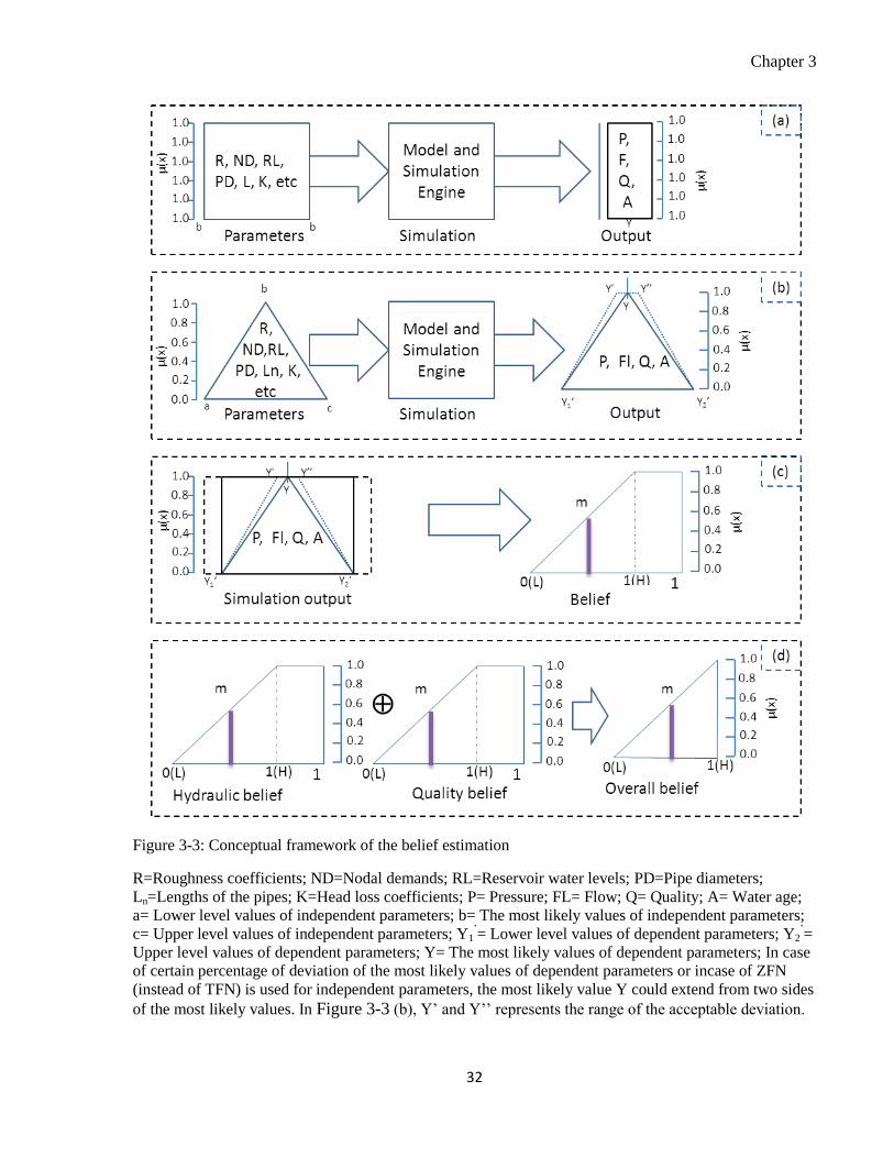
Chapter 3

32

Figure 3-3: Conceptual framework of the belief estimation

R=Roughness coefficients; ND=Nodal demands; RL=Reservoir water levels; PD=Pipe diameters;

Ln=Lengths of the pipes; K=Head loss coefficients; P= Pressure; FL= Flow; Q= Quality; A= Water age;

a= Lower level values of independent parameters; b= The most likely values of independent parameters;

c= Upper level values of independent parameters; Y1’= Lower level values of dependent parameters; Y2

’=

Upper level values of dependent parameters; Y= The most likely values of dependent parameters; In case

of certain percentage of deviation of the most likely values of dependent parameters or incase of ZFN

(instead of TFN) is used for independent parameters, the most likely value Y could extend from two sides

of the most likely values. In Figure 3-3 (b), Y’ and Y’’ represents the range of the acceptable deviation.

Chapter 3

33

The solution of a calibrated model estimates the values of dependent parameters (for all nodes and

pipes) under normal condition, whereas the other two set solutions estimate the two sets of the

possible extreme values of dependent parameters (for all nodes and pipes). Details of the different

steps are discussed in the following sections. The EPANET (Rossman 2000) simulation engine and

the source codes have been used for simulations. Different stages of the proposed methodology and

the EPANET toolkits’ functions have been implemented using MATLAB 7.10 (MathWorks 2010).

Identification and Fuzzification of Independent Parameters 3.2.1

A water supply system is a spatially distributed complex infrastructure. To model numerically such

an infrastructure requires to model many parameters, such as pipe diameters, lengths, and roughness

coefficients, nodal demands, water levels in reservoirs and pump characteristic curves, and

performance characteristics of different valves and minor elements (Gupta and Bhave 2007). Among

those parameters, some are relatively easy to measure and model such as pipe lengths, some are very

difficult to measure and modelling of these parameters uncertain such as roughness coefficients, and

some are in between, such as nodal demand, for which a statistical distribution can be generated if

enough information is available (Revelli and Ridolfi 2002). These parameters have varying degrees

of impacts on WSS operations. The parameters which are relatively difficult to estimate , hence

uncertain, and have significant impact on WSS simulation results have been modeled as uncertain

parameters and modelled as fuzzy numbers. However, modelling of all WSS independent parameters

as uncertain parameter will not reduce the reliability of the results; however, it will increase the

computational burden. Roughness coefficients, nodal demands, and reservoir water levels are

considered the most common parameters which are imprecise and may have a significant impact on

the hydraulic (Gupta and Bhave 2007; Revelli and Ridolfi 2002) and water quality results. Therefore,

these three parameters can be selected as the most influential network independent parameters.

After the selection of independent parameters, the most likely and the extreme values of the selected

parameters are defined. The values of independent parameters of a calibrated model can be used as

the best estimate for the most likely values. The extreme values can be assumed based on reported

literature values, industry experiences, and other supporting data or can be assumed as certain

percentages of the most likely values. Based on the minimum, the most likely and the maximum

values of all the selected independent parameters, fuzzification has been carried out. To fuzzify the

data, generally triangular fuzzy numbers (TFN) or trapezoidal fuzzy numbers (ZFN) are used (Lee

Chapter 3

34

1996). All the selected parameters (e.g., roughness coefficients, nodal demands, reservoir water

levels) have been fuzzified in order to belong to the corresponding set presented by Equation 3-1:

[ ] [3-1]

where X is the possible range of a variable x (network independent parameters) and µx is the

membership function of x. Figure 3-4 shows the TFN and ZFN, and Equations 3-2 and 3-3 fuzzify

the data in terms of TFN and ZFN, respectively.

( )

{

( )

( )

( )

( )

[3-2]

( ) {

( )

( )

( )

( )

[3-3]

Figure 3-4: Triangular and trapezoidal fuzzy numbers

For a TFN, a is the minimum value, b is the most likely value and c is the maximum value of an

independent parameter. For a ZFN, a is the minimum value, d is the maximum value and b and c are

the two values which represent the interval of the most likely values.

Although the fuzzy independent parameters are strictly triangular or trapezoidal with linear sides

(e.g., ab’ and b’c for TFN and ab’ and c’d for ZFN), the corresponding fuzzy dependent parameters

will be also triangular or trapezoidal but with curvilinear sides (e.g., ab’ and b’c for TFN and ab’ and

c’d for ZFN; See Figure 3-4), because of the nonlinearity of the system (Revelli and Ridolfi 2002).

0

0.2

0.4

0.6

0.8

1

f(x

)

TMF

ZMF

a b c d

b' c'

Chapter 3

35

However, the difference between the linear and the curvilinear sides is negligible (Gupta and Bhave

2007). Therefore, the fuzzy numbers for dependent parameters have been considered triangular or

trapezoidal with linear sides. For this study, the triangular fuzzy number has been used. We assume

that the fuzzified values of the independent parameters are in an Nx3 matrix [a b c], where N is the

number of an independent parameter. Two types of dependent parameters are evaluated. Nodal

pressure has been used a hydraulic dependent parameter whereas residual nodal chlorine

concentration has been used as quality dependent parameter.

Estimation of Extreme Values of Dependent Parameters 3.2.2

To estimate the extreme values of the dependent parameters, it is required to define all the fuzzy

independent parameters. The following steps are used to estimate the extreme values of dependent

parameters:

1. Estimate the dependent parameters for the normal values of independent parameters [b] using

EPANET. We assume, [Y] is the matrix of the simulated dependent parameters.

2. Change the first element of the matrix [b] with its maximum value from the matrix [c] (matrix of

the maximum values of independent parameter), keeping all other elements of the matrix [b] the

same.

3. Use EPANET to estimate the dependent parameters for the changed set of independent

parameters. We assume that the results of dependent parameters are reported as [Dn] = [D1].

4. Reset all the independent parameters to their normal condition.

5. Repeat steps 2 to 4 for all the independent parameters.

6. Estimate the difference [C] = [Dn] - [Y] for the simulated dependent parameters.

7. Maximize the first dependent parameter under the following conditions: If any element of the

matrix [C] is greater than 0 (C>0), then the corresponding changed independent parameters

should be maximum and if C<0 then the corresponding changed independent parameters should

be a minimum value. The selected set of maximum and minimum independent parameter matrix

(Mx) will produce the first maximum dependent parameter.

8. Run the simulation for the selected combination of extreme independent parameters and select

the first maximum dependent parameter.

Chapter 3

36

9. Repeat steps 7 and 8 for all the dependent parameters.

10. Minimize the first dependent parameter under the following conditions: If any element of the

matrix [C] is greater than 0 (C>0), then the corresponding changed independent parameters

should be minimum value and if C<0 then the corresponding changed independent parameters

should be maximum value. The selected set of minimum and maximum independent parameter

matrix (My) will produce the first minimum dependent parameter.

11. Run the simulation for the selected extreme independent parameters and select the first

minimum dependent parameters.

12. Repeat steps 10 and 11 for all the dependent parameters.

13. Repeat steps 1 to 12 for different time steps.

Based on the steps, the extreme values of the hydraulic dependent parameters for 24 hours can be

estimated. However, the extreme values of the water quality dependent parameters require certain

modifications in step 6 of the above algorithm. There is a difficulty in the steady state water quality

solution using EPANET. Water quality simulation requires extended period simulation (EPS). In the

EPS water quality simulation, the quality time steps are much shorter than the hydraulic time steps to

accommodate shorter travel times that can occur within a pipe (Rossman 2000). In EPANET, the

default hydraulic time step is one hour whereas default quality time step is just five minutes which

have been castoff in the current study. In step 6, a single value of dependent parameter is compared

to check the monotonicity for steady state hydraulic simulation. However, for water quality

simulation, the corresponding values are compared for extended period simulation considering

monotonicity in EPS. During the comparison, it is noticed that changes of water quality parameter

for the change of independent parameters are very small and the changes are monotonic with a

certain exception. For a particular node, approximately, 95-to 99% times, the water quality results

show the monotonicity. About 1-5% times, nodal water quality parameters show no changes or

reverse changes in very small magnitude which could be resulted from numerical instability of the

EPANET computational engine. For simplicity, in this study, the impact of independent parameters

on water quality dependent parameters is considered monotonic. The extreme values of water quality

parameters (e.g., residual chlorine concentration) estimated in a similar way as extreme values of

hydraulic depended parameters are estimated with a modification in step 6.

Chapter 3

37

For the WSS example (Figure 3-1), fuzzy dependent parameters have been estimated considering

±0.5 m variation in the reservoir level (i.e., 27.5m, 28m, and 28.5m as the minimum, most likely and

maximum value, respectively), ±5 variation in roughness coefficients (i.e., 95, 100, 105), and ±5%

variation in nodal base demands from their normal values. Following above mention steps, the

possible maximum, the most likely and the minimum values of pressure at different nodes have been

estimated (Table 3-3) under steady state condition.

Table 3-3: Maximum, most likely & minimum pressure values at different nodes (base demand)

Node

ID

Pressure, m

Minimum Most likely Maximum

A 26.15 26.86 27.46

B 25.75 26.51 27.14

C 25.70 26.47 27.10

D 24.24 25.26 26.00

Using the above algorithm, EPS values for pressure and water quality parameters (e.g., chlorine)

concentration can be estimated.

Reliability Estimation 3.2.3

The reliability of a WSS for a customer is the utility related to customers’ satisfaction. A customer

will be satisfied when the desirable water is available to him with a desired quantity with desired

pressure, and desired quality. Therefore, WSS reliability has been evaluated based on the customers’

satisfaction received for the services from a WSS, and expressed in terms of customers’ utilities. The

utility has been used as a measure of reliability. If a customer received guaranteed desired utility

from a WSS with 100% satisfaction under any condition, then the WSS is considered fully reliable

and vice versa. The customer utilities from a WSS are depended on the available water volume,

pressure and quality. Although the nodal pressure and the available water volume are strongly

interrelated, however, both are independently important to a customer. A customer receiving water

with low pressure and a customer receiving the same volume of water with high pressure do not have

a same level of satisfaction. Therefore, the hydraulic utility has been divided into demand utility and

pressure utility.

Chapter 3

38

3.2.3.1 Pressure Utility

In the WSS reliability assessment literature, most of the investigators assumed that if the available

pressure in a node is higher than the desired level of service then the node is fully reliable and if

available pressure is less than the desired level of service, then a zero reliability (Gupta and Bhave

1994). However, some authors consider a linear distribution of hydraulic reliability in terms of

hydraulic availability in the range of minimum accepted pressure level and desired pressure level. At

the minimum pressure level, the hydraulic reliability is assumed to zero and at the desirable pressure

level, it is full and in between the minimum and the desired pressure level, the reliability is expressed

in terms of different functions (Fujiwara and Ganesharajah 1993).

Similar to the traditional reliability, in this study, utility is considered zero when the pressure is equal

or less than the accepted minimum level of pressure and full utility when pressure is equal or higher

than the desired level of service. In between these two pressures, utilities are linearly interpolated.

Figure 3-5 shows the distribution of pressure utility at a particular node at a particular time. Equation

3-4 has been used to model the pressure utility from a particular node at a particular time.

Des

jj

Des

jj

mLoS

jmLoS

j

Des

j

mLoS

jj

mLoS

jj

j

PP,1

PPP,)PP(

)PP(

PP,0

)p(U

[3-4]

where, Uj (p) is the pressure utility at a node j at a particular time, t; Pj is pressure a node j at a

particular time, t under normal condition; PjmLos is the minimum level of service in terms of pressure,

Pjdes is the desired pressure.

Figure 3-5: Distribution of pressure utility

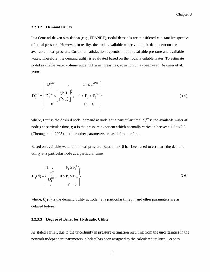
Chapter 3

39

3.2.3.2 Demand Utility

In a demand-driven simulation (e.g., EPANET), nodal demands are considered constant irrespective

of nodal pressure. However, in reality, the nodal available water volume is dependent on the

available nodal pressure. Customer satisfaction depends on both available pressure and available

water. Therefore, the demand utility is evaluated based on the nodal available water. To estimate

nodal available water volume under different pressures, equation 5 has been used (Wagner et al.

1988).

0P0

PP0,)P(

)P(D

PP,D

D

j

Des

jj

n

1

Des

jDes

j

Des

jj

Des

j

avl

j

[3-5]

where, DjDes is the desired nodal demand at node j at a particular time; Dj

avl is the available water at

node j at particular time, t; n is the pressure exponent which normally varies in between 1.5 to 2.0

(Cheung et al. 2005), and the other parameters are as defined before.

Based on available water and nodal pressure, Equation 3-6 has been used to estimate the demand

utility at a particular node at a particular time.

0P0

PP0,D

D

PP,1

)d(U

j

desjdes

j

av

j

des

jj

j

[3-6]

where, Uj (d) is the demand utility at node j at a particular time , t, and other parameters are as

defined before.

3.2.3.3 Degree of Belief for Hydraulic Utility

As stated earlier, due to the uncertainty in pressure estimation resulting from the uncertainties in the

network independent parameters, a belief has been assigned to the calculated utilities. As both

Chapter 3

40

available pressure and available demand are directly pressure dependent, therefore, a single belief

function, termed as “hydraulic belief” has been used. Equation 3-7 has been used to estimate the

belief of the estimated hydraulic utility (pressure and demand utility).

L

j

Des

j

H

jj

L

jL

j

H

j

j

H

j

H

j

mLoS

j

j

PP,1

PPP,)PP(

)PP(

PP,0

)hu(

[3-7]

where, µj (hu) is the belief in the calculated hydraulic utility at node j at a particular time, t; PjL and

PjH are the estimated lowest pressure and highest pressure at the particular node, j (section 3.2.2 )

and at a particular time, t, respectively, and other parameters are as defined before.

3.2.3.4 Water Quality Utility

If a customer receives guaranteed desired quality water from a node under any condition then the

node is considered has full water quality utility. If the quality of water dropped from the desired level

to the minimum acceptable level than the water quality utility also drops from full utility to zero

water quality utility. If the water quality lies in between desired and minimum required quality level

then the water quality utility is interpolated between 0 and 1. Although, water quality is a function of

various physical, chemical and microbiological parameters, however, for this study, only residual

chlorine concentration in the available water has been used as a measure of water quality utility. If

fact, residual chlorine is one of the best cost/benefit indicators of the variability of water quality in a

WSS (Fisher et al. 2011).

Figure 3-6: Distribution of water quality utility

Chapter 3

41

Four levels of chlorine concentrations, namely, the minimum level of concentration (QjmLoS ), the

lower level of the desired concentration (QjlDes), the upper level of the desired concentration (Qj

uDes )

and the unacceptable level of service (QjuLoS ), have been used to define water utility from a residual

chlorine concentration (Figure 3-6). As a low level of chlorine concentration makes the favorable

environment in WSS for different microorganisms regrowth and biofilm formation (Lund and

Ormerod 1995), water quality utility has been considered zero after a minimum threshold chlorine

concentration. Similarly, as the excessive chlorine concentration is not desirable in drinking water,

an upper level of desired chlorine concentration (QjuDes ) and an unacceptable level of chlorine (Qj

uLoS

), have been considered. If the residual chlorine concentration in the available water is higher than

the upper level of the desired concentration (QjuDes), the excessive chlorine favors reaction with

natural organic matter (NOM) which produces potentially harmful chlorinated by-products and

offensive taste and odor to the consumers (Fisher et al. 2011). Therefore, the water quality utility

starts to reduce and will totally diminish to zero if the chlorine concentration reached to the

unacceptable level of service (QjuLoS). Equation 3-8 has been used to model water quality utility for a

particular node at a particular time.

uDes

jj

lDes

j

uDes

jj

uLoS

juDes

j

uLoS

j

j

uLoS

j

lDes

jj

mLoS

jLoS

jdes

mLoS

jj

uLoS

jj

mLoS

jj

j

QQQ,1

QQQ,)QQ(

)QQ(

QQQ,)QQ(

)QQ(

QQorQQ,0

)q(U

[3-8]

where, Uj (q) is the water quality utility at node j at time, t ; Qj is the water quality at normal

condition at node j at time, t; QjmLoS is the minimum level of service, Qj

lDes is the lower level of

desired level of service ; QjuDes is the upper limit of desired (full utility if the chlorine concentration

lies in between QjlDes and Qj

uDes); and QjuLoS is the maximum level concentration that generates water

quality utility. Concentration higher than this level has no water quality utility.

3.2.3.5 Degree of Belief for Water Quality Utility

Similar to the estimated hydraulic utility, estimated water quality utility subjected to uncertainties

and a degree of belief has been incorporated in the evaluated water quality utility. Similar to the

Chapter 3

42

hydraulic utility belief, Equation 3-9 has been used to estimate the degree of belief of the calculated

water quality utility at a particular node at a particular time.

L

j

mLoS

j

H

jj

L

jL

j

H

j

j

H

j

H

j

mLoS

j

j

QQ,1

QQQ,)QQ(

)QQ(

QQ,0

)qu(

[3-9]

where, µj (qu) is the degree of belief to water quality utility at node j at time, t; QjL is the estimated

lowest water quality (section 3.2.2 ) at a particular node j at time, t; QjH is the estimated highest water

quality (section 3.2.2 ) at node j at time, t, and the other parameters are as defined before.

3.2.3.6 Cumulative Utility

Based on the estimated demand utility, pressure utility and water quality, the aggregated utility at a

node at a particular time has been estimated. Various aggregation operators (Sadiq and Manuel J.

Rodriguez 2005) could have been used to aggregate the estimated different kinds of utilities. To meet

all the requirements, t-norm (‘AND’-type) operators are necessary to be used. However, if a single

parameter is enough to meet the criteria, a t-conorm (‘OR’-type) operator can be used. To meet all

the utility requirements, it is required to fulfill pressure utility, demand utility and water quality

utility criteria at all times, therefore, a t-norm operator has been used. However, the pressure utility

and the demand utility are strongly interrelated. Equation 3-10 has been used to estimate the

hydraulic utility at a particular node, j at particular time, t combining the pressure and demand

utilities.

)()()( dUpUhuU jjj

[3-10]

where Uj (hu) is the hydraulic utility at junction j at time, t; Uj (p) is the pressure utility at node j at a

particular time, t; Uj (d) is the demand utility at node j at a particular time, t.

To combine hydraulic utility and quality utility, maximum of t-norm, “AND” operators has been

used (Equation 3-11).

)(),(min)( quUhuUcU jjj

[3-11]

Chapter 3

43

where Uj (c) is the combined utility at junction j at time, t; and other parameters are as defined as

before.

Equation 3-12 has been used to estimate the aggregated belief of the combined utility.

)()()( quhuc jjj

[3-12]

where µj (c) is combined belief at junction j at time, t; and other parameters are as defined before.

3.2.3.7 General Solutions

Figure 3-7 shows the general solution domain for the reliability solutions based on the proposed

methodology. It is noted that a utility without a belief and a belief without a utility are not practical,

therefore, no solution exits along the both axes (BC and CD), except a solution at origin (0, 0). In

addition, a full belief is not possible without a full utility, therefore, no solution exists along the top

border line, AB, except a solution at the top right corner A (1, 1). Except these three boundary lines,

conceptually, a solution can exist anywhere in the solution domain including along the right

boundary line, AD. A solution at the bottom half of Figure 3-7(region Y) where belief is always

below 0.5 has actual reliability less than the reliability estimated by traditional reliability assessment.

This is because, if there is no uncertainty with different independent parameters, estimated belief will

be always 0.5 which is the basic assumption in the traditional approach. However, a solution in the

upper half of Figure 3-7 (region X) has the degree of belief higher than the traditional reliability

estimates.

Figure 3-7: General solution domain

Chapter 3

44

For a new WSS, designed reliability should stay in the region X. A solution at the top right corner A

(1, 1) represents the absolute reliability of the system. A solution other than this point subjected to

the uncertainties. Therefore, for a system where a high reliability is necessary, such as a WSS to

supply water to a hospital or to a nuclear power plant, the solution should stay at the top right corner

of Figure 3-7 (i.e., at point A (1, 1)). In addition, the higher the uncertainties in the estimate, the

lower the belief of the calculated utilities without changing the estimated utilities. To demonstrate

this phenomenon, the example network has been solved with an average reservoir level of 26 m and

±0.5 and ±1.0 m reservoir level variations.

Figure 3-8 shows the hydraulic reliabilities at different times in a day under two different levels of

uncertainties (reservoir level variations ±0.5 and ±1.0 m). From

Figure 3-8, it is evident that with increased uncertainties in the independent parameters, the solution

moves down from the absolute reliability position indicating the lower beliefs to the calculated

utilities.

Figure 3-8: Hydraulic reliability at Node D under different level of uncertainties

0.5

0.52

0.54

0.56

0.58

0.6

0.62

0.5 0.6 0.7 0.8 0.9 1 1.1

Bel

ief,

µ (

hu)

Hydraulic Utility, U(hu)

1m reservoir level variation

0.5 m reservoir level variation

Chapter 3

45

Table 3-4: EPS reliability results for Node D of the example network

Time, hr. Pressure, m Demand, , m3/h Utility Residual Chlorine, mg/l Quality Combined

Max. Normal Min. Base Available Pressure Demand Belief Max. Normal Min. Utility Belief Utility Belief

(1) (2) (3) (4) (5) (6) (7) (8) (9) (10) (11) (12) (13) (14) (15) (16)

0-2 26.05 25.51 24.92 4.94 4.94 1.00 1.00 0.52 0.67 0.67 0.67 1.00 1.00

1.00 0.72

2-4 26.01 25.46 24.86

5.19 5.19

1.00 1.00 0.52

0.62 0.62 0.62

1.00 1.00

1.00 0.72

4-6 24.40 23.70 22.76

11.38 11.07

0.87 0.97 0.57

0.57 0.57 0.57

1.00 1.00

0.92 0.75

6-8 21.25 20.22 18.63

18.69 16.81

0.52 0.90 0.61

0.53 0.53 0.53

1.00 1.00

0.69 0.78

8-10 22.62 21.73 20.42

15.88 14.80

0.67 0.93 0.60

0.57 0.56 0.56

1.00 1.00

0.79 0.77

10-12 22.89 22.04 20.79

15.25 14.32

0.70 0.94 0.59

0.57 0.57 0.57

1.00 1.00

0.81 0.77

12-14 23.98 23.23 22.21

12.56 12.11

0.82 0.96 0.58

0.57 0.56 0.56

1.00 1.00

0.89 0.76

14-16 24.53 23.84 22.93

11.00 10.74

0.88 0.98 0.57

0.56 0.55 0.55

1.00 1.00

0.93 0.75

16-18 23.19 22.36 21.17

14.56 13.77

0.74 0.95 0.59

0.55 0.54 0.54

1.00 1.00

0.83 0.77

18-20 23.11 22.27 21.07

14.75 13.92

0.73 0.94 0.59

0.55 0.55 0.54

1.00 1.00

0.83 0.77

20-22 23.47 22.67 21.54

13.88 13.21

0.77 0.95 0.58

0.56 0.56 0.55

1.00 1.00

0.85 0.76

22-24 24.36 23.65 22.71

11.50 11.19

0.86 0.97 0.57

0.56 0.55 0.55

1.00 1.00

0.92 0.75

Note: Assigned initial nodal residual chlorine concentrations high enough to ensure desired residual chlorine concentration for the first few hours

at different nodes (Shaded)

Chapter 3

46

Using the developed methodology, different utilities for the example network under the normal

operating condition have been estimated. Table 3-4 shows the EPS reliability (24 hours) results for

node D of the example network (Figure 3-1).

From the column (15) and (16), it is evident that in no time interval the WSS is absolutely reliable. If

pressure, demand and water quality utilities are considered separately, as per traditional reliability

assessment method, the WSS system will be fully reliable in some points of the day. However, due to

the uncertainty in the different independent parameters, the beliefs on calculated utilities are matters

of concern.

It is noted that if the initial residual chlorine concentrations at different nodes start at zero, it takes up

to 8 hours to reach a residual chlorine concentration to the critical node. During these hours, the

water quality utility at critical node is very small or zeros. To avoid these zero utility, an initial

residual chlorine concentration is assigned at each node which ensures the desired concentration at

each node for the first few hours (Shaded part of Table 3-4). In a real WSS, this does not happen as

the WSS supplies water after enough water flushing and if the network is simulated for an existing

operating condition, initial residual chlorine concentration will show up from the beginning of the

simulation.

3.2.3.8 System Utility

Estimated pressure, demand, and water quality utilities provide a snapshot utility of different nodes

at a particular time. However, these estimated utilities cannot provide utility as a whole to a WSS.

Therefore, the overall system utility is estimated to evaluate the performance of the system as a

whole. The overall system utility is defined as a utility received from a WSS as a whole over a

certain period of time. Equation 3-13 has been used to estimate the overall aggregated system utility

for a particular time. In this equation, desired demand has been used as weighted factors for the

aggregated system utility.

N

j

Des

j

N

j

j

Des

j

t

D

cUD

suU

1

1

)(

)(

[3-13]

Chapter 3

47

where, all the parameters have their usual meaning as defined previously.

For an aggregated utility over a period of time, Equation 3-14 has been used. In this equation, desired

system demand over the period has been used as a weighted factor in the aggregation.

T

t

T

t

T

t

j

T

t

D

suUD

suU

0

0

)(

)(

[3-14

where, DtT= total desired system demand over the period of time, and all the other parameters have

their usual meaning as defined before.

The belief of the aggregated utility function has been defined in a similar way. Equation 3-15 has

been used to estimate the overall belief of the calculated system utility for a particular time and

Equation 3-16 has been used to estimate the overall system belief of calculated system utility.

N

1j

av

j

N

1j

j

av

j

j

D

)C(D

)s(

[3-15]

where, all the parameters have their usual meaning as defined before.

T

t

Tot

t

T

t

t

Tot

t

D

CD

s

1

0

)(

)(

[3-16]

where, DtTot= total available water for the whole WSS over the period and all the other parameters

have their usual meaning as defined before.

Table 3-5 shows the system utility, and the system belief of the example WSS in normal operating

condition. From Table 3-5, it is noticed that the absolute reliability was not achieved at any time,

even in normal operating condition. Although, at time 0-4am, estimated system utility was one but

Chapter 3

48

due to the degree of belief which is less than one, it is not possible to consider as an absolute

reliability.

Table 3-5: System utility for Example WSS

Time,

hr.

System

Utility

System

Belief

0-2 1.000 0.907

2-4 1.000 0.908

4-6 0.966 0.741

6-8 0.815 0.765

8-10 0.883 0.757

10-12 0.896 0.755

12-14 0.947 0.746

14-16 0.971 0.740

16-18 0.910 0.753

18-20 0.907 0.753

20-22 0.924 0.750

22-24 0.964 0.742

Overall 0.917 0.762

3.3 Model Implementation and Demonstration

To demonstrate the applicability of the proposed methodology, the developed model has been

implemented and demonstrated through a case study. The example WSS represents a simplified

version of a part of a WSS (Islam et al. 2011b).

Figure 3-9 shows the layout of the example WSS with node and link numbers and pipe lengths. The

example WSS has 27 nodes connected by 40 pipes with a total length of 19.5 km. Water is supplied

by gravity from the two elevated reservoirs (reservoir 1 and reservoir 2) with the total head of 90 m,

and 85 m, respectively. The lengths of the pipes vary from 100 m to 680 m, and the diameters of the

pipes vary from 200 mm to 700 mm. The base demand at different nodes varies from 50 l/s to 100

l/s, and the demand multipliers ranges from 0.38 at 5am to 1.46 at 9 am. To estimate available initial

residual chlorine concentration at both reservoirs are assumed at 0.80mg/l.

Chapter 3

49

Figure 3-9: Layout of the study example WDS (pipe length not to the scale)

Detail information on pipe length, diameter, roughness coefficient, nodal connectivity, and nodal

hourly base demand and demand multipliers2 and two reservoirs head have been provided in Table

3-6.

2 In hydraulic network modelling, base demand is the demand that the modelers assign to any

particular node. For steady state simulation, it does not change. However, water demand changes

continuously over time. To incorporate this change in demand, demand multipliers have been used.

This is the ratio of demand at any time to base demand.

1

200 2

600

3

500

4

100

5

500

6

600

7

400

8

300

9

600

10

650

11

300

12

500

13

500

14

460

15

600

16

500

17

400

18

650

19

600

20

350

21

500

22

600

23

500

24

500

25

450

26

400

27

600

28

650

29

400

30

600

31

450

32

450

33

400

34

500

35

450

36

680

37

450

38

500

39

550

40

560

3 4 5

6 7 8 9 10

11 12 13 14 15

16 17 18 19 20

21 22

23 24 25

26 27

1 2

Length

1

1

1

1

m

Chapter 3

50

Table 3-6 : Information of the example WDS

Node Information Pipe information DM

Node Id BD (l/s) Pipe

Id

U/S

Node

D/S

Node

L

(m)

D

(mm)

R Hr MF

3 83.3 1 1 3 200 700 100 1 0.41

4 100.0 2 3 4 600 600 100 2 0.38

5 66.7 3 4 5 500 600 95 3 0.38

6 66.7 4 2 5 100 675 100 4 0.45

7 50.0 5 3 7 500 675 100 5 0.83

8 133.3 6 4 8 600 600 95 6 1.53

9 83.3 7 5 9 400 650 100 7 1.46

10 83.3 8 7 6 300 300 90 8 1.30

11 100.0 9 7 8 600 450 95 9 1.24

12 66.7 10 9 8 650 450 95 10 1.28

13 100.0 11 9 10 300 300 100 11 1.14

14 50.0 12 6 11 500 250 85 12 0.87

15 83.3 13 7 12 500 500 95 13 0.89

16 50.0 14 8 13 460 500 95 14 0.87

17 100.0 15 9 14 600 500 95 15 1.06

18 50.0 16 10 15 500 250 110 16 1.21

19 50.0 17 12 11 400 300 100 17 1.15

20 100.0 18 12 13 650 400 90 18 1.18

21 50.0 19 13 14 600 400 85 19 1.04

22 83.3 20 14 15 350 300 90 20 1.06

23 83.3 21 11 16 500 250 90 21 0.87

24 50.0 22 12 17 600 400 110 22 0.70

25 83.3 23 13 18 500 450 90 23 0.60

26 66.7 24 14 19 500 400 95 24 0.40

27 50.0 25 15 20 450 250 100

26 17 16 400 300 105

27 18 17 600 350 100

28 18 19 650 400 95

Node Information 29 19 20 400 300 100

Res. ID Head (m) 30 16 21 600 200 100

1 90 31 17 22 450 300 90

2 85 32 18 23 450 300 95

33 19 24 400 300 85

BD=Base demand; L=Length; D=Diameter; R=Roughness; DM= Demand multiplier; MF =

Multiplying factor

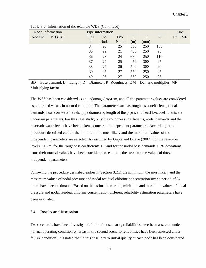
Chapter 3

51

Table 3-6: Information of the example WDS (Continued)

Node Information Pipe information DM

Node Id BD (l/s) Pipe

Id

U/S

Node

D/S

Node

L

(m)

D

(mm)

R Hr MF

34 20 25 500 250 105

35 22 21 450 250 90

36 23 24 680 250 110

37 24 25 450 300 95

38 24 26 500 300 90

39 25 27 550 250 95

40 26 27 560 250 95

BD = Base demand; L = Length; D = Diameter; R=Roughness; DM = Demand multiplier; MF =

Multiplying factor

The WSS has been considered as an undamaged system, and all the parameter values are considered

as calibrated values in normal condition. The parameters such as roughness coefficients, nodal

demands, reservoir water levels, pipe diameters, length of the pipes, and head loss coefficients are

uncertain parameters. For this case study, only the roughness coefficients, nodal demands and the

reservoir water levels have been taken as uncertain independent parameters. According to the

procedure described earlier, the minimum, the most likely and the maximum values of the

independent parameters are selected. As assumed by Gupta and Bhave (2007), for the reservoir

levels ±0.5 m, for the roughness coefficients ±5, and for the nodal base demands ± 5% deviations

from their normal values have been considered to estimate the two extreme values of those

independent parameters.

Following the procedure described earlier in Section 3.2.2, the minimum, the most likely and the

maximum values of nodal pressure and nodal residual chlorine concentration over a period of 24

hours have been estimated. Based on the estimated normal, minimum and maximum values of nodal

pressure and nodal residual chlorine concentration different reliability estimation parameters have

been evaluated.

3.4 Results and Discussion

Two scenarios have been investigated. In the first scenario, reliabilities have been assessed under

normal operating condition whereas in the second scenario reliabilities have been assessed under

failure condition. It is noted that in this case, a zero initial quality at each node has been considered.

Chapter 3

52

From the calculated results, it reveals that under the normal condition, the WSS has the capabilities

to provide enough water with desirable quality and desirable pressure during the period of

simulation. It is also observed that in all cases the desired level of water volume, water pressure, and

quality of water always higher than the minimum values of pressure and quality (except first three

hours of operation). Therefore, it can be concluded that the WSS has absolute reliability in normal

condition during the period of simulation.

According to the definition of reliability, reliability assessment under normal condition is not enough

to understand the performance of a WSS under emergency condition. Therefore, reliability

assessments are necessary under all possible extreme conditions. This also includes failure of

multiple pipes at a time including the failure of the reservoir connection line during the fire event,

and power or pumping station failure. Although an unlimited number of failure scenarios are

possible, however, the probability of multiple pipe failures at the same time is very low (Tabesh et al.

2001). It can be assumed that pipe failures are independent (Su et al. 1987). In addition, if any

dependency exists, it will be the negative dependency. For example, if a pipe failure happens in the

system, it will reduce the pressure in the system and due to reduced system pressure, the probability

of another pipe failure will reduce. However, in case of large WSS, the influence of pressure might

not be significant. Other pipe failure factors, such as vandalism, traffic loading may cause the pipe

failures which are totally independent events. As the purpose of this article is to demonstrate a novel

methodology for reliability assessment, all the possible failure scenarios have not been investigated.

For this study one pipe failure at a time is assumed. In addition, no fire demand is considered. There

are various techniques and methods available to estimate the probability of pipe failure, time for

repairs, and mean time between the failures (MTBF). Interested readers are suggested to read the

chapter 18 of Mays (2000). In this study, randomly one pipe failure at a time has been generated

using a uniform distribution in the range of [1, N] where N is the pipe number. The reliability

assessment has been carried out only for one day. Therefore, the impacts of repair time and repair

interval have not been investigated. However, these parameters are very important aspects of WSS

reliability assessment.

From the analysis of pressure, flow and residual chlorine concentration over the simulation period, it

is found that the most critical node in the network is node 27. This node received minimum pressure

at all times. As stated earlier, during the normal operating condition, the hydraulic utility and the

degree of belief at all time steps are always unit which indicates that absolute reliability under

Chapter 3

53

normal condition. The uncertainties in the network independent parameters can not influence the

hydraulic utility of the system. However, after initial chlorine concentration reached to the most

critical point (i.e., after 3 hours network operation), the water quality utility for the WSS is also one.

Analyzing different pipe failure scenarios, it is found that the most critical node (i.e., node 27)

received the minimum pressure and the minimum residual chlorine concentration when the pipe 4 is

disconnected from the network. This is also justified as the node 27 is the furthest node from the both

sources, and this node is only connected by two pipes. Figure 3-10 shows that the available pressure

at the identified critical node 27 under different pipe break situations. Due to the lack of considerable

chlorine demand in the network, no considerable effect was observed in the residual chlorine

concentrations.

Figure 3-10: Available pressure at critical point under critical pipe failure condition

Chapter 3

54

Table 3-7: EPS reliability results for Node 27 of the example network

Time,

hr.

Pressure, m Demand, m3/h Utility Residual Chlorine,

mg/l Quality Cumulative

Max. Normal Min. Base Available Pressure Demand Belief Max. Normal Min. Utility Belief Utility Belief

(1) (2) (3) (4) (5) (6) (7) (8) (9) (10) (11) (12) (13) (14) (15) (16)

0-2* 83.16 82.52 81.17

19.75 19.75

1.00 1.00 1.00

0.00 0.00 0.00

0.00 0.00

0.00 0.00

2-4* 82.44 81.81 80.42

20.75 20.75

1.00 1.00 1.00

0.52 0.41 0.35

0.64 0.61

0.64 0.78

4-6 56.01 54.92 50.62

45.50 45.50

1.00 1.00 1.00

0.75 0.74 0.73

1.00 1.00

1.00 1.00

6-8 4.02 2.03 -8.00

74.75 21.28

0.00 0.28 0.00

0.77 0.77 0.76

1.00 1.00

0.00 0.00

8-10 26.56 24.96 17.42 63.50 63.45 1.00 1.00 0.82 0.77 0.77 0.76 1.00 1.00 1.00 0.91

10-12 31.15 29.62 22.59

61.00 61.00

1.00 1.00 0.82

0.77 0.77 0.76

1.00 1.00

1.00 0.91

12-14 49.05 47.84 42.77

50.25 50.25

1.00 1.00 1.00

0.77 0.76 0.76

1.00 1.00

1.00 1.00

14-16 58.09 57.03 52.96

44.00 44.00

1.00 1.00 1.00

0.76 0.76 0.76

1.00 1.00

1.00 1.00

16-18 36.01 34.57 28.07

58.25 58.25

1.00 1.00 1.00

0.77 0.76 0.76

1.00 1.00

1.00 1.00

18-20 34.70 33.24 26.60

59.00 59.00

1.00 1.00 1.00

0.77 0.77 0.76

1.00 1.00

1.00 1.00

20-22 40.68 39.32 33.33

55.50 55.50

1.00 1.00 1.00

0.77 0.76 0.76

1.00 1.00

1.00 1.00

22-24 55.31 54.20 49.83 46.00 46.00 1.00 1.00 1.00 0.76 0.76 0.76 1.00 1.00 1.00 1.00

* In this case, the network has been simulated with zero initial quality because of modelling complexities. In a real WSS, it does not happen

as the initial residual chlorine concentration will show up from the beginning of the simulation.

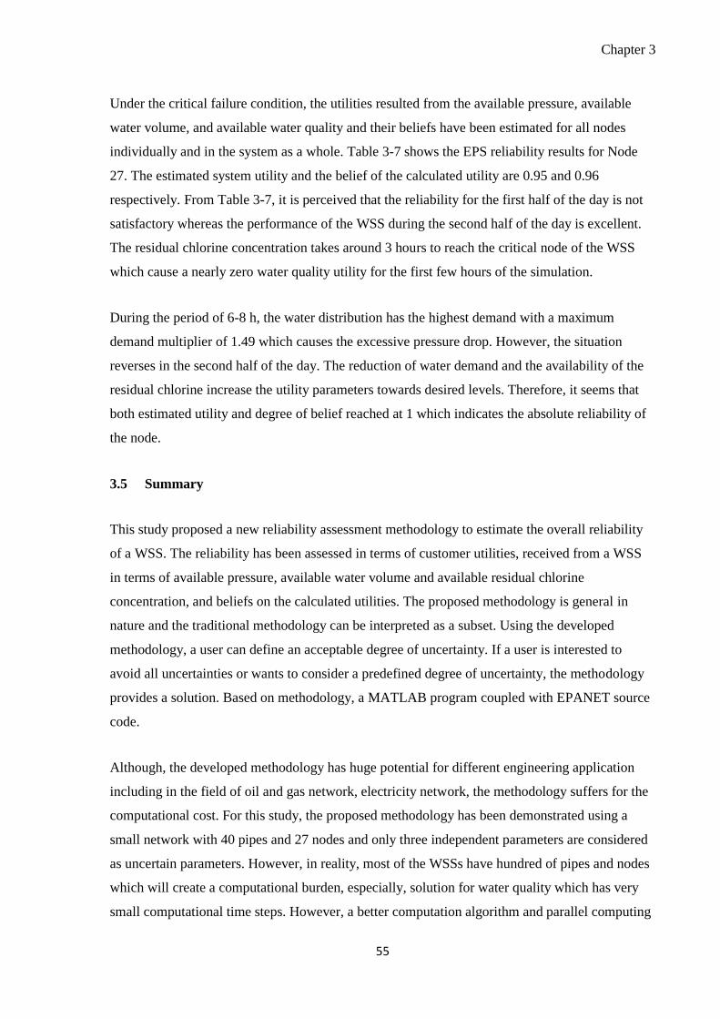
Chapter 3

55

Under the critical failure condition, the utilities resulted from the available pressure, available

water volume, and available water quality and their beliefs have been estimated for all nodes

individually and in the system as a whole. Table 3-7 shows the EPS reliability results for Node

27. The estimated system utility and the belief of the calculated utility are 0.95 and 0.96

respectively. From Table 3-7, it is perceived that the reliability for the first half of the day is not

satisfactory whereas the performance of the WSS during the second half of the day is excellent.

The residual chlorine concentration takes around 3 hours to reach the critical node of the WSS

which cause a nearly zero water quality utility for the first few hours of the simulation.

During the period of 6-8 h, the water distribution has the highest demand with a maximum

demand multiplier of 1.49 which causes the excessive pressure drop. However, the situation

reverses in the second half of the day. The reduction of water demand and the availability of the

residual chlorine increase the utility parameters towards desired levels. Therefore, it seems that

both estimated utility and degree of belief reached at 1 which indicates the absolute reliability of

the node.

3.5 Summary

This study proposed a new reliability assessment methodology to estimate the overall reliability

of a WSS. The reliability has been assessed in terms of customer utilities, received from a WSS

in terms of available pressure, available water volume and available residual chlorine

concentration, and beliefs on the calculated utilities. The proposed methodology is general in

nature and the traditional methodology can be interpreted as a subset. Using the developed

methodology, a user can define an acceptable degree of uncertainty. If a user is interested to

avoid all uncertainties or wants to consider a predefined degree of uncertainty, the methodology

provides a solution. Based on methodology, a MATLAB program coupled with EPANET source

code.

Although, the developed methodology has huge potential for different engineering application

including in the field of oil and gas network, electricity network, the methodology suffers for the

computational cost. For this study, the proposed methodology has been demonstrated using a

small network with 40 pipes and 27 nodes and only three independent parameters are considered

as uncertain parameters. However, in reality, most of the WSSs have hundred of pipes and nodes

which will create a computational burden, especially, solution for water quality which has very

small computational time steps. However, a better computation algorithm and parallel computing

Chapter 3

56

can increase the computational performance of the proposed methodology which has not been

addressed in this study. This study was especially focused on a novel integrated reliability of a

WSS. However, integration of reliability, robustness and resilience (K. Zhang et al. 2012) of a

WSS can be investigated in the future.

Chapter 3

57

CHAPTER 4 LEAKAGE POTENTIAL MODEL

A version of this chapter has been published in the Journal of Water Supply: Research and

Technology – AQUA on 22th March 2012 with the title “Evaluating Leakage Potential in Water

Distribution Systems: A Fuzzy-Based Methodology” (Islam et al. 2012a).

4.1 Introduction

It is stated earlier that leakage from WDS is a universal problem around the globe-only the

difference in volume. The latest global water supply and sanitation assessment report (WHO-

UNICEF-WSSCC 2000) estimated that the typical value of non-revenue water in Africa, Asia,

Latin America and Caribbean and in North America are 39%, 42%, 42% and 15% respectively.

One of the main components of these is lost water through leakages (M. Farley and Trow 2003)

There is no single reason for occurrence of leakage in any WDS. There could be numerous

physical, environmental and hydraulic factors that pose threats or make WDSs vulnerable to

cause leakage. Different external (to the network) factors, network physical components,

workmanship quality, network operating practices directly or indirectly influence the leakage.

Among external factors, such as traffic loading, influences the pipe failure due to vibration and

heavy loading over the buried pipes. Soil types and its permeability influence the length of time a

leak is allowed to continue as well as leakage flow rate. Groundwater table and temperature

influence the moisture contents which may have potential impacts on the breakage and leakage

(M. Farley 2001). Physical components like number of service connections, number of water

meters, number of joints, material of the physical components, different type of demands and

many others influence leakage significantly (M. Farley 2001; A. Lambert 2002; Tabesh et al.

2009). Factors like operating system pressure and the age of network (i.e., age of pipes and

network components if they are not explicitly mentioned) increase the leakage rate (Fares and

Zayed 2009). Similarly, the poor workmanship of different network components like meters,

valves and pumps can be significant contributors to leakage in WDSs (Furness 2003).

To assess the effect of each factor on the leakage in WDSs, it is necessary to have a good

monitoring system and huge amount of data. It is also necessary to have well established water

leakage detection and management system which are quite uncommon in most of the small-sized

WDSs, or even in many bigger systems in the developing countries. However, the utility

Chapter 3

58

managers of those communities always want to have the tools and techniques to understand the

impacts of different factors on leakage and leakage potential (LP) of their distribution systems.

As mentioned in the literature review, there are significant numbers of studies (Fares and Zayed

2009; Jowitt and Xu 1993; Kleiner et al. 2004; Rogers and Grigg 2006; Sadiq et al. 2004; Yamini

and Lence 2009) have also been reported in the literature that discussed the concepts related to

WDS’s reliability. However, most of these studies focus on the failure of the WDS integrity.

Very little research has been reported for evaluating LP of any WDS. For example, Klusman

(2002) proposed a methodology for evaluation of the LP in a carbon dioxide EOR3/sequestration

project. However, no significant literature has been reported for evaluating LP for WDS.

This research employed the concept of risk to assess the leakage potential. As defined earlier, risk

is a product of likelihood of an undesirable event, i.e., the probability of occurrence of the event,

and its related consequences (Sadiq et al. 2004). The definition of consequence is a vague

concept. There are numerous ways to model the consequence of any undesirable phenomenon.

The consequence modelling is generally carried out in terms of socio-economic impact, human

health loss, asset loss, and environmental impact (Arunraj and Maiti 2009). However, in this

study, consequences have not been modelled rather only the likelihood or leakage ‘potential’ has

been modelled. The scale of ‘potential’ is used as a continuous interval of [0 1] or [0 100%]. The

terms ‘probability’, ‘possibility’, ‘risk’ and even ‘likelihood’ have been intentionally avoided to

avert confusion. The term ‘possibility’ or ‘likelihood’ refers to what can happen whereas

‘probability’ refers to what will happen. Moreover, the terms ‘possibility’ and ‘likelihood’ have

specific meanings in Bayesian theory and Possibility theory (Sadiq et al. 2010). But the essence

of the term ‘potential’ is very similar to the ‘possibility’ or ‘likelihood’. A 100% LP of a WDS

means that the production volume and LP are same in that WDS. If 100% LP becomes effective

to any WDS, then no water will be travelled to the tap of any customer. Using the concepts of

risk and fuzzy logic/fuzzy set theory, this research aims at developing a new tool for water utility

managers for evaluating LP in different parts of WDS under limited data and resources. The tool

will help them to prioritize their active leakage control (ALC) and rehabilitation strategies. The

output of this model is a significant part of the developed integrated prognostic and diagnostic

analysis framework.

3 Enhanced Oil Recovery (EOR) is a generic term used for expressing techniques for increasing the amount

of crude oil that can be extracted from an oil field

Chapter 3

59

It is important to note that the detectable pipe failure and leakage are not synonymous. All

detectable failures are the subset of leakage, however, without any detectable failure a huge

volume of background leakage can exist in any WDS. Considering their time of awareness,

identification of their locations and time of repair, this kind of background leakage is the most

important component of total leakage volume in any WDS (Farley 2001).

4.2 Leakage Potential Model Development Methodology

The proposed methodology requires identification of different leakage influencing factors and

aggregation of those factors under varying operating system pressure. To aggregate the influences

of each factor, a hierarchical relationship structure has been developed. Fuzzy rule-based (FRB)

inferencing system has been used to aggregate the influences of each factor. To model the

behavior of different influencing factors under varying operating system pressure, a pressure

adjustment factor (PAF) has been developed and incorporated in with the aggregation process.

Model Framework 4.2.1

Figure 4-1 shows the hierarchical structure of leakage influencing factors and their

interrelationship. The structure consists of four levels or generations of factors. The LP is in the

first generation whereas the basic contributory factors are either in the third or fourth generation.

An extensive literature survey was carried out to identify these factors which contribute to the

leakage in WDSs. Based on the literature survey (e.g., Fares and Zayed 2009; Farley 2001; Farley

and Trow 2003; Lambert 2001; Lambert et al. 1999; May 1994) and state-of-the practice

information, a list of 24 basic factors has been identified which directly (e.g., pressure) or /and

indirectly (e.g., traffic movement) influences the leakage. The interrelationships among various

basic and dummy factors have been expressed using Meta language developed by Sadiq et al.

(2007, 2004). Each element of the hierarchical structure has been expressed as Xi,jk ,where, X

represents the leakage influencing factors, i represents the child, j for parent and k denotes the

generation of the basic influencing factors. Both basic (for which data can be obtained) and

dummy or intermediate (derived based on basic factors) factors in a hierarchical structure are

composed of a “parent” and “children” relationships. Factor with no parents is the total “LP for

the system” and factors with no children are the basic leakage influencing factors.

Chapter 3

60

Leakage Potential in Pipe

X1,01

Pip

e

Att

rib

ute

, X

1,3

3

Pip

e M

ate

ria

l

Pip

e

Dia

me

ter

Lo

ad

ing

Tra

ffic

Flo

w

Co

ve

r D

ep

th

Wo

rkm

an

sh

ip,

X5,1

2

Pip

e

Pla

ce

me

nt

Be

dd

ing

an

d

Ba

ck

fill

Co

mp

ac

tio

n

Pip

e

Wo

rkm

an

sh

ip,

X2,5

3

Ne

t. In

str

u.

Wo

rkm

an

sh

ip

Jo

ints

, M

ete

rs,

SC

s,

X2,3

3

Tra

ffic

Im

pa

ct,

X1,1

3

Ph

ys

ica

l,

X3,1

2

Ex

tern

al, X

1,1

2

Gro

un

d

Co

nd

itio

n

Imp

ac

t, X

2,1

3

De

ma

nd

, X

3,3

3

Re

sid

en

tia

l

Co

me

rcia

l

Ind

us

tria

l

X1,53

X1,14

X2,14

X3,14

X7,14

X8,14 X12,3

4X13,3

4X14,3

4 X14,24

X15,24

X16,24

So

il T

yp

e

GW

Ta

ble

Flu

ctu

ati

on

Te

mp

era

ture

Flu

ctu

ati

on

X4,24

X5,24

X6,21

Nu

mb

er

of

Se

rvic

e

Co

nn

ec

tio

ns

Nu

mb

er

of

Wa

ter

Me

ters

Nu

mb

er

of

Jo

ints

Ge

ne

rati

on

1 Xi,jk

ParentChild

Generation

Ge

ne

rati

on

2G

en

era

tio

n 3

Ge

ne

rati

on

4

Ag

e, X

4,1

2

Pip

e A

ge

Ne

t.

Ins

tru

me

nt

ag

e

X1,43

X2,43

Pre

ss

ure

, X

2,1

2

Sy

ste

m

Pre

ss

ure

He

ad

los

s

X1,23

X2,23

X9,24

X10,24

X11,24

Figure 4-1: Hierarchical structure of selected leakage influencing factors

Chapter 4

61

Among 24 factors, the influence of 22 basic factors, except pressure exponent4 and reference

pressure, can be propagated through these four generations. Pressure exponent and reference

pressure influence LP taking part in the calculation of pressure adjustment factor provided in

section 4.2.3. The first generation parent LP has five children in second generation namely

external, pressure, physical, age and workmanship. Like their parent each of the five factors has

their own children in the third generation. The parent factor “external” has two children namely

traffic impact and ground condition impact. The parent factor “pressure” has two children namely

system pressure and head loss which are basic factors. The parent factor “physical” has three

children namely pipe attribute, joints, meters and service connections and demand. The parent

factor “age” has two children namely pipe age and network instruments’ age which are basic

factors. Network instrument workmanship and pipe workmanship are the children of

workmanship; network instrument workmanship is a basic factor.

All third generation children except which are basic factors (children of age and pressure) have

children in the fourth generation. Parent traffic impact has three basic children in fourth

generation namely loading, traffic flow and cover depth. Similarly, the ground condition impact

has three basic children: soil type, temperature fluctuation and ground water table fluctuation.

Pipe materials and pipe diameter are the children of pipe attribute while number of water meters,

number of joints and number of service connections are the children of joints, meters and

connections. Residential, commercial and industrial are three children of demand and finally pipe

placement, bedding and backfill, and compaction are three children of pipe workmanship. All

factors in the fourth generation are basic influencing factors.

After the development of LP framework, the research methodology is divided into two main

parts; namely, fuzzy rule based (FRB) modelling and adjustment of pressure for calculating LP

for varying operating system pressure profiles. In the first part of the methodology, FRB

modelling has been carried out and in the second part, a pressure adjustment factor (PAF) has

been calculated to model the influence of different factors under varying pressure conditions.

Calculated PAF has been incorporated within FRB modelling by multiplying with the output of

basic influence factors. Each part of the methodology has multiple stages. Details of the stages

have been presented in the following sections. All stages have been implemented by using

4 Leakage flow rate is proportional to a power (exponent) relationship of system pressure (Equation 4-19). The

power (exponent) of the pressure of that relationship is termed as pressure exponent.

Chapter 4

62

MATLAB 7.9 Fuzzy Inferencing Toolbox together with the MATLAB traditional coding

environment (Fuzzy Logic Toolbox 2- User’s Guide 2011).

Fuzzy Rule Based (FRB) Modelling 4.2.2

Fuzzy sets are used to deal with vague and imprecise information (Zadeh 1965) . Fuzzy set theory

is widely applied to solve real-life problems that are subjective, vague, and imprecise in nature

(Smithson and Verkuilen 2006; Yang and Xu 2002). It provides a strict mathematical framework

in which vague conceptual phenomena can be studied precisely and rigorously (Zimmermann

2001). Since its conceptualization, it has been used in various engineering applications including

civil engineering. It is successfully implemented for the structural damage analysis, vibration

control of flexible structure, cement rotary kiln, concrete analysis and design (Gad and Farooq

2001). Sadiq et al. (2007) implemented fuzzy logic for predicting water quality failures in WDS.

There are numerous other examples for the application of fuzzy logic in water distribution

modelling. Four steps are required to implement FRB modelling: fuzzification, inferencing,

defuzzification and normalization (interpretation). Figure 4-2 shows the sequence of information

flow for FRB modelling.

Figure 4-2: Information flow in FRB modelling

4.2.2.1 Fuzzification

Fuzzification is a step that transforms all commensurate or non-commensurate data into a

homogeneous scale by assigning memberships with respect to predefined linguistic variables

(Chowdhury et al. 2007; Khan and Sadiq 2005).

Chapter 4

63

Table 4-1: Fuzzy sets and linguistic definition of input parameters

Reference Figure: T1 Reference Figure: T2

Inputs Symbol Interval Ref. Fig. (1) (2) (3) (4) (5) (6) (7) (8)

LD X1,14 0-300 T1 0 0 150 300 300 300

FL X2,14 0-30000 T1 0 0 15000 30000 30000 30000

CD5 X3,1

4 5-0 T1 0 0 0.9 2 5 5

ST6 X4,2

4 0-100 T1 0 0 30 60 100 100

TF X5,24 0-20 T1 0 0 6 12 20 20

GF X6,21 0-10 T1 0 0 3 6 10 10

NM X9,24 0-100 T1 0 0 30 60 100 100

NS X10,24 0-100 T1 0 0 30 60 100 100

NJ X11,24 0-50 T1 0 0 15 30 50 50

RD7 X12,3

4 0-1 T1 0 0 0.5 1 1 1

CoD X13,34 0-1 T1 0 0 0.5 1 1 1

InD X14,34 0-1 T1 0 0 0.5 1 1 1

PP8 X14,2

4 0-1 T1 0 0 0.5 1 1 1

BB X15,24 0-1 T1 0 0 0.5 1 1 1

C X16,24 0-1 T1 0 0 0.5 1 1 1

PM9 X7,1

4 0-1 T1 0 0 0.5 1 1 1

PD X8,14 0-10 T1 0 0 0.3 0.72 10 10

SP X1,23 0-100 T2 0 0 25 50 75 100 100 100

HL X2,23 2-0 T1 0 0 0.25 0.5 2 2

PA X1,43 0-100 T2 0 0 25 50 75 100 100 100

IA X2,43 0-100 T2 0 0 25 50 75 100 100 100

LD=Traffic loading (KN); FL= Traffic flow (Vehicle/h); CD=Cover depth (m); ST=Soil Type (% finer); TF= Temperature

fluctuation (0C); GF=Ground water table fluctuation (m); NM=(Number of )water meters; NS= (Number of )service

connection; NJ= (Number of) joints; RD=Residential demand; InD=Industrial demand; CoD=Commercial demand; PP=

(Quality of) pipe placement; BB= (Quality of) bedding and backfills; C=Quality of compaction; PM= Pipe materials;

PD=Pipe diameter (m); SP=System pressure, m; HL=Head loss (m/km); PA= Pipe age (yr)IA= Network instrument age( yr).

5 Cover depth and head loss has reverse relationship with LP. Therefore, in Figure T1 the ‘Low’ should be read as the ‘High’

and the ‘High’ should be read as the ‘Low’)

6 Soil type defined by percentage finer than 0.002 mm

7 All the demands are relative to pressure drop. If pressure drop due to demand is high, then demand is consider as a high

value and vice versa

8 Low placement quality considered when pipe placement is carried out by unskilled technicians with no engineering

supervision and high placement quality when placement is carried out by skilled technician with engineering supervision.

Same is considered for Bedding and Backfills and for Compaction.

9 Assumed low value for metallic (DI, ST,GI, CI etc.) pipes, medium value for plastic (HDPE, PE, PVC etc.) pipes and high

value for others(PC, AC, etc.) pipe materials

Thresholds

Chapter 4

64

To fuzzify data, generally triangular fuzzy numbers (TFN) or trapezoidal fuzzy numbers (ZFN)

are used to represent linguistic variables (Lee 1996). For this study, all the leakage influencing

factors have been modelled using TFN and ZFN (Figure 3-4). Equations 3-2 and 3-3 (Chapter 3)

have been used to model the TFN and ZFN.

Definitions of a, b, c, d for different leakage influencing factors in different granularity levels

have been presented in the form of thresholds shown in Figure T1 and T2 attached with the Table

4-1. To define fuzzy numbers, threshold values need to be read based on the values defined in

Table 4-1. For each ZFN, first, second, third and fourth values are a, b, c, and d respectively.

However, for TFN, the fourth value is out of consideration. For each leakage influencing input,

type of fuzzy number and threshold values (eventually, a, b, c and d) are based on the literature

review (e.g., Fares and Zayed 2009; Farley 2001; Farley and Trow 2003; Lambert 2001; Lambert

et al. 1999; May 1994) and contacting experts from water industry.

Most of the membership functions have three levels of granularity which are expressed through

linguistic variables: low, medium and high. However, for some relatively more sensitive input

factors and their output (e.g., pressure, age), 5-level granularity for membership functions (very

low, low, medium, high and very high) is defined (Figure 4-3). The final LP output function has

also 5-level of granularity. For example, Figure 4-3 shows a fuzzified value of pressure 45m with

the following degree of memberships ( ): very low (0), low (0.2), medium (0.78), high (0) and

very high (0).

Figure 4-3: Five level granularity of fuzzy numbers

0

0.2

0.4

0.6

0.8

1

0 10 20 30 40 50 60 70 80 90 100

Mem

ber

ship

Val

ue

Qualitative Scale (0-100)

Very Low Low Medium High Very High

Chapter 4

65

4.2.2.2 Fuzzy Inferencing System

In FRB modelling, the relationships between fuzzy variables are represented by if-then rules of

the form “If antecedent proposition then consequent proposition”. In a linguistic model where

both the antecedent and consequent are fuzzy propositions, the rule can be written as (Mamdani,

1997):

Ri: If x is Ai then y is Bi; i = 1, 2, …, k [4-1]

The antecedent x (input) and the consequent y (output) are linguistic variables whereas Ai and Bi

are linguistic constants. The truth-value (real number) of these propositions depends on the

degree of similarity between the variables and the constants. The values of x and y belong to

fuzzy sets in their respective domains, whereas Ai and Bi are selected from sets of prescribed

terms. The rule R = {Ri/i = 1, 2, …, k} and the sets A and B constitute the knowledge base of the

linguistic model. A fuzzy rule is a restriction on the simultaneous occurrence of x and y; Ri (X

Y) [0, 1]. The fuzzy conjunction Ai Bi can be computed using a minimum operator (t-norm)

as follows (Mamdani, 1997):

Ri = Ai Bi i.e., Ri (x, y) = Ai (x) Bi (y) [4-2]

The minimum operator is computed on the Cartesian X-Y product space for all possible pairs of x

and y. The fuzzy relation R represents the entire model and is given by the disjunction (union or

maximum, i.e., s-norm) of k individual relations of the Ri rule, as follows:

R =

)()(),(.,.,1

1

yxmaxyxeiR BiAiki

R

k

i

i

[4-3]

The fuzzy relation R encodes the entire rule-base and allows computation of the model output

using the max-min composition (o) according to the following equation:

y = x o R [4-4]

For an input fuzzy value x = A′, an output value B′ is given by the following composition:

),()(max)( '' yxxy RAX

B [4-5]

Chapter 4

66

Substituting R (x, y) from Equation 4-5, the above expression takes the following form:

' '1

( ) max ( ) max ( ) ( )( )B A Ai Bii kX

y x x y

[4-6]

The above equation is rearranged as follows:

' '1

( ) max max[ ( ) ( )] ( )( )B A Ai Bii k X

y x x y

[4-7]

Assuming )()(max ' xx AiA

Xi

is the degree of fulfillment of the ith rule antecedent.

The resulting output fuzzy set of the linguistic model is of the following form:

'1

( ) max ( ) ,B i Bii k

y y y Y

[4-8]

To obtain a crisp output, defuzzification of fuzzy set elements can be performed using quality

ordered weights (wl). Denoting m as the number of output granules, B’l (y) as the output

membership for each output granule (Equation 4-8), and Bol as the crisp representative value of

each output granule, defuzzification is conducted as follows (Yang and Xu 2002):

l

m

l

lOlBO wByy

1' )(

[4-9]

Details on defuzzification have been described in next section of this article. The fuzzy rule-

based model is trained (fine-tuned) on a given experimental dataset to find quality ordered

weights (wl). The training can be performed using linear optimization of an objective function

2min Oobs yyAvg

, which is a minimization of the square root of the mean square error

(SRMSE), denoting yobs as the observed value, yo as the modeled value (Equation 4-9). The

above algorithm is known as a single-input single-output (SISO) model, which could be extended

to a multiple-input single-output (MISO) model as follows:

Ri: If x1 is A1i and x2 is A2i and…and xp is Api then y is Bi; i = 1, 2, .., k [4-10]

Chapter 4

67

This model is a special case of Equation 4-1, as the set Ai is obtained by the Cartesian product of

fuzzy sets Ai = A1i A2i A3i... Api. Hence the degree of fulfillment (i) becomes:

1 21 2( ) ( ) ... ( );i pA i A i Apix x x i = 1, 2, .., k [4-11]

Subsequent details are identical to those of SISO (Yager and Filev 1994). Two fuzzy rule-based

inferencing methods are very common: the Mamdani and the Takagi, Sugeno and Kang (TSK)

methods. The Mamdani method is the most common in practice and connects antecedents to

consequents through a rule set, whereas the TSK method provides a systematic approach to

generating fuzzy rules from an input-output function (Ross 2004).

For the present study, Mamdani algorithm has been implemented. This algorithm was proposed

by Mamdani and Assilian (Ross 2004). In this methodology, the MISO model is of the form:

Ri: If x1 is A1i and x2 is A2i and…and xpi is Api then yi is Bi; i = 1, 2, ..., k [4-12]

where A1i, A2i, … Api are the fuzzy set representing the ith antecedent vector-values, and Bi is the

fuzzy set representing the ith consequent.

In the max-min inference (it can also be referred as Mamdani and Assilian max-product

inference), the degree of fulfillment (βi) and the aggregated output for the k Bi y), are

respectively:

[ , , , ]i A1i 1 A2i 2 Api p min x x x [4-13]

[ [ , , , ]]Bi A1i 1 A2i 2 Api pi

(y) max min x x x ; i = 1, 2, … k [4-14]

Using the quality ordered weights (wl) and the centroid (C) of each consequent linguistic constant

(output granule); m being the number of granules and Bl (y) the membership for each granule; a

crisp value of the output variable resulting from defuzzification can be computed for the ith

consequent as follows:

1

mMam

i Bl l l

l

y (y) C w

; i = 1, 2, …, k [4-15]

Chapter 4

68

4.2.2.3 Defuzzification

Defuzzification is a procedure for determining the crisp value which is considered the most

representative of the fuzzy set output taken as an isolated entity (Saade and Diab 2002). Several

methods of defuzzification exist, e.g., the centre of gravity (COG), bisector, mean of maximum,

smallest of maximum and largest of maximum. COG technique is the most popular due to its

simplicity and easiness for programming, less use of computer resource and a reasonable output

(Fares and Zayed 2009). Therefore, this study also applies COG method. The value of the crisp

LP value has been calculated following the equation:

∑

∑

[4-16]

where, Ar is the truncated area taken from membership function based on inferencing rules, Dck is

the moment arm of the truncated area and k is the membership function.

4.2.2.4 Normalization

For absolute favorable condition, the calculated LP should be close to zero and for absolute

unfavorable condition the calculated LP should be close to the unit value. However by using

COG method, it is impossible to obtain these two extreme values due to the nature of the

approximation. Therefore, produced results using this method could be confusing to the people

who are not familiar with the method. To avoid this confusion and to make easier interpretation

of the results, the calculated crisp value has been normalized between 0 and 1 by using Equation

4-17:

[4-17]

where LPN is the normalized LP for any condition; LPcog is the LP for any condition calculated

by COG method;

is the minimum LP for extreme favorable condition calculated by COG

method; and

is the maximum LP for extreme unfavorable condition calculated by COG

method.

Chapter 4

69

Pressure Adjustment 4.2.3

Pressure is the most important factor that influences the leakage flow rates (Farley 2001). It also

affects other leakage influencing basic factors ( Farley 2001; Farley and Trow 2003; Lambert

2001). To model the relationship between pressure and other influencing factors, a pressure

adjustment factor (PAF) has been proposed to reflect the influence of pressure to all pressure

dependent basic inputs. If ρGG-1 is the outputs for the influencing factors of the generation Gth,

ρGG-1 will serve as input for the upper generation, i.e. generation Gth-1. The proposed PAF has

been applied to the outputs (ρGG-1) under the condition of (ρG

G-1) × PAF ≤ 1. Then the influence of

pressure will be propagated to the final crisp LP according to the structure earlier provided in

Figure 4-1.

There are four main steps to calculate the proposed PAF. Firstly, it is necessary to select the

“reference system pressure”. The term “reference system pressure” is the pressure above which

leakage and break frequency increases more rapidly. At this level, pressure initiates to influence

the other leakage influencing factors. For a system with continuous supply, leakage and break

frequency increases rapidly when pressure exceeds around 35 to 40 meters (50 to 57.1 psi) of

head (Lambert, 2001; Farley and Trow, 2003). Therefore a reference system pressure could be

between 35 m to 40 m (50 to 57.1 psi) of head. However, the value of reference system pressure

could change based on the network condition, age of network, design standards and other factors.

After selection of reference system pressure, it is necessary to select the average operating system

pressure. If the proposed model is intended to apply to an individual pipe, the average operating

system pressure should be calculated as an average of upstream and downstream pressure of the

pipe. However, if the model intended to apply to a whole or part of WDS, then average operating

system pressure should be selected in such a way that it represents the average operating system

pressure of the whole or part of WDS, respectively.

Third, it is necessary to estimate the pressure exponent (N1) which generally varies between 0.50

and 2.50, depending upon the type of leakage path, network age, corrosion, materials and other

network related factors (Farley and Trow 2003). However, maximum values in excess of 2.5

reported in field tests (Farley and Trow 2003) are also realistic (Greyvenstein and Van Zyl 2007).

For larger detectable leakage from plastic pipes, typical N1 value could be 1.5 or even higher,

while larger detectable leakages in the metal pipe could have N1 value close to 0.5 (Lambert

2001). Greyvenstein and Van Zyl (2007) found a value of pressure exponent 2.3 in a steel pipe

Chapter 4

70

with extensive corrosion damage to the pipe wall and having reduced supporting material

surrounding the leak openings.

Finally, this research developed a special FRB model based on the approach discussed in the

section 4.2.2. For this special model, pressure is considered only influencing factor and hence

defined rules for this model is only pressure dependent (SISO model). For example, if pressure is

low then LP is low; if pressure is high then LP is high. Figure 4-4 shows the LP model

considering pressure as the only influencing factor.

Figure 4-4: LP evaluation considering only the pressure as an influencing factor

The model has been then used to determine LP for estimated reference system pressure (LPRP)

and LP for estimated operating system pressure (LPSP). Based on estimated LPRP, LPSP and the

pressure exponent N1, PAF is calculated by using Equation 4-18:

(

)

[4-18]

The relationship of Equation 4-18 is based on the general relationship between pressure and

leakage. According to Lambert (2001) the appropriate relationship between leakage and pressure

can be expressed by following two equations

Chapter 4

71

[4-19]

(

)

[4-20]

where L represents the leakage volume per unit time, P represents the pressure, P0 is the

reference system pressure, L0 is the leakage rate for the reference system pressure, P1 is the

system pressure at any time, L1 is the system leakage for Pressure P1 and N1 is the pressure

exponent.

4.3 Example Evaluation of Leakage Potential

To demonstrate the actual process of the developed model as described previously, an example

evaluation process has been described below. The example shows, how the different inputs

contributed to the overall leakage potential evaluation.

Step 1: Hierarchical model (Figure 4-1)

Step 2: Data collection (Table 4-3)

Step 3: Calculation of pressure adjustment factor (PAF10):

From Table 4-3, Operating system pressure (SP) =12.56 m (17.94 psi); Reference pressure (RP) =

25 m (35.71 psi) and N = 1.16. For SP<RP, no influence of pressure to other factors is

considered. Therefore PAF = 1.

However, for demonstration purpose, calculation of PAF for SP = 35 m (50 psi) where SP>RP

has been shown as follow:

Step 3.1: Input and output fuzzy membership function for pressure dependent SISO model

(Figure 4-5)

10

For all abbreviation please read main thesis

Chapter 4

72

Figure 4-5: Input and output fuzzy membership functions for pressure dependent SISO model

Step 3.2: Rules for pressure dependent SISO model

R1: If pressure is low then LPRP-LPSP11 is low)

R2: If pressure is medium then LPRP-LPSP is medium

R3: If pressure is high then LPRP-LPSP is high

Step 3.3: Rule evaluation and outputs (Figure 4-6)

Figure 4-6: Rules evaluation and outputs for RP and SP

11

Evaluate LPRP when input variable is reference pressure (RP) and evaluate LPSP when input variable is

operating system pressure (SP)

Chapter 4

73

Step 3.4: PAF calculation

Defuzzified output for RP (LPRP) = 0.516 and Defuzzified output for SP (LPSP) = 0.65.

Therefore (

)

(

)

Step 4: Fuzzification of basic inputs

There are 24 basic factors (22 factors are fuzzified and 2 factors are incorporated with PAF).

Only for demonstration purpose, inputs for Joints, Meters, SCs (X2,33) group has been shown.

Step 4.1: Input and output membership function for Pressure only SISO model

Figure 4-7: Input and output membership function for MISO model

Step 4.2: Rules for MISO model (Figure 4-7)

R1: If NM is low and NS is low and NJ is low then NM-NS-NJ is low

R2: If (NM low) and (NS low) and (NJ medium) then (NM-NS-NJ is low)

Chapter 4

74

R3: If (NM low) and (NS low) and (NJ high) then (NM-NS-NJ is medium)

......................................................................................................................

......................................................................................................................

R26: If (NM high) and (NS high) and (NJ medium) then (NM-NS-NJ is low)

R27: If (NM high) and (NS high) and (NJ high) then (NM-NS-NJ is high)

Step 4.3: Rule evaluation and outputs (Figure 4-8)

Figure 4-8: Rules evaluation and outputs for NM, NS and NJ

Defuzzified output from pressure independent NM, NS and NJ= 0.58

Step 4.4: Normalization

Maximum impact for extreme unfavorable conditions from NM, NS and NJ without

normalization using COG method: 0.837.Minimum impact for extreme favorable conditions from

NM, NS and NJ without normalization using COG method: 0.1633

Therefore, normalized impact:

Chapter 4

75

Step 4.5: Incorporation of PAF

Pressure dependent input in third generation as Joints, Meters, SCs (X2,33) = 0.619×PAF =

0.619×1 = 0.5812.

Step 5: Steps 4 has been repeated for other fourth generation inputs. Resulting third generation

dummy inputs for traffic impact(X1,13), ground condition impact(X2,1

3), pipe attribute (X1,33),

demand (X3,33), pipe workmanship (X2,5

3) and joints, meters, SCs (X2,33) are 0.444, 0.333, 0.484,

0.517 , 0.551 and 0.58 respectively. In the generation, there are four basic inputs which are

system pressure (SP), head loss (HL), pipe age (PA) and network instrument age (IA). The values

of these basic inputs are obtained from Table 4-2.

Step 6: Using inputs obtained in step 5, FRB inferencing has been carried out. The output

obtained for the generation Gth (3rd generation for example) will be the input for the generation

Gth-1 (i.e., 2nd generation). Resulting second generation dummy inputs for external (X1,12),

pressure (X2,12) , physical ( X3,1

2), age( X4,12), workmanship(X5,1

2) are 0.494, 0.147,0.587,0.202

and 0.493 respectively. It is noted that in this case no pressure adjustment has been carried out

except for age. However, normalization has been carried out as step 4.4.

Step 7: Using dummy inputs obtained in Step 6, FRB inferencing has been carried out to estimate

final normalized crisp value of leakage potential (LP). For this case, dummy inputs obtained in

Step 6 have been fuzzified using TFN. Dummy parameters external (X1,12), physical(X3,1

2) have

two levels of granularity (i.e., low and high) and age( X4,12), workmanship(X5,1

2) and pressure

(X2,12) have three level of granularity (i.e., low, medium and high). However, the output final LP

has five level of granularity (i.e., very low, low, medium, high and very high). Number of rules

applied for this part of modelling is 108 (3×3×3×2×2). Typical rules used are shown as

following:

R1: If External is low and Physical is low and Workmanship is low and Pressure is low

and Age is low then LP is low

..........................................................................................................................................

..........................................................................................................................................

R107: If External is high and Physical is high and Workmanship is high and Pressure is

high and Age is medium then LP is high

12

If( X2,33 )×PAF>1 then assumed X2,3

3 = 1.

Chapter 4

76

R108: If External is high and Physical is high and Workmanship is high and Pressure is

high and Age is high then LP is very high

Using this FRB model estimated leakage potential before normalization is 0.484. This defuzzified

has been normalized similar as step 4.4. However, for this case, maximum impact for extreme

unfavorable conditions from external, physical, workmanship, pressure and age without

normalization using COG method: 0.92 and Minimum impact for extreme favorable conditions

from external, physical, workmanship, pressure and age without normalization using COG

method: 0.08.

Normalized leakage potential:

Therefore, final normalized crisp value of leakage potential (LP) is 0.481 or 48%.

4.4 Application of Proposed Leakage Potential Model

This study proposed a model that can be implemented to an individual pipe, or to a part of the

network or to the whole WDS. The extent of application depends on the degree of accuracy

required for a particular case and spatial variability of the influencing factors. If the spatial

variability of different leakage influencing factors is very high, developed model should be

implemented in each pipe of the network. In this case, all the network instruments (i.e., joints,

service connections, water meters, fixtures, fittings, etc.) located on the pipe are needed to be

considered as a part of the pipe. A special attention should be given to avoid duplication of any

network instrument. Each pipe will have a separate LP and those can be presented as LP map of

the WDS. However, if the spatial variability of different leakage influencing factors is relatively

small, the developed model can then be implemented in the network as a whole and therefore a

crisp value of the LP will be evaluated for the whole WDS.

Study Area– Bangkok’s Metropolitan Water Authority 4.4.1

To evaluate the practicality of this research, the model has been implemented for a small district

metering area (DMA) of the Metropolitan Water Authority (MWA) of Bangkok (Thailand). The

MWA is responsible to supply good quality water to its consumers (residences, businesses, and

industries) in Bangkok and its surrounding provinces of Nonthaburi, and Samut Prakan (Figure

4-9). The water supply system consists of 15 service areas with 14 branch offices and one

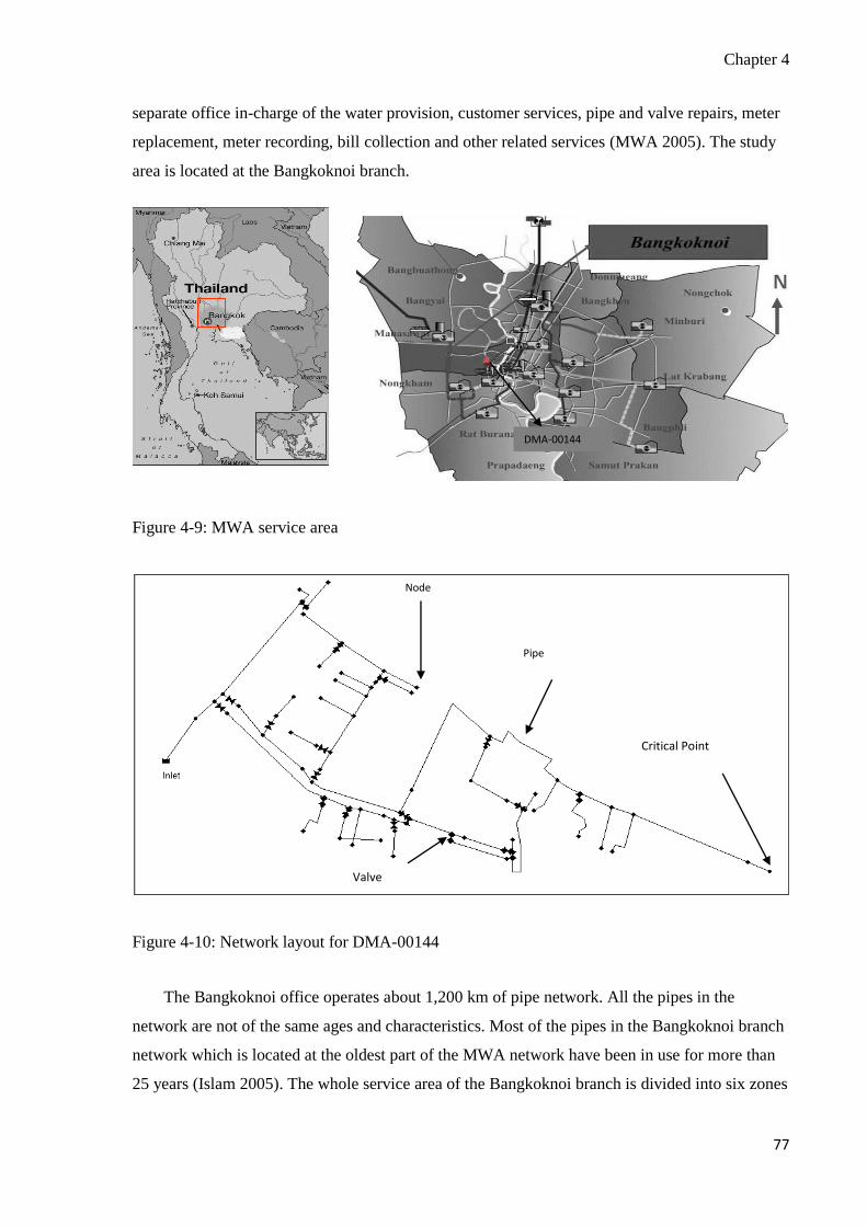
Chapter 4

77

separate office in-charge of the water provision, customer services, pipe and valve repairs, meter

replacement, meter recording, bill collection and other related services (MWA 2005). The study

area is located at the Bangkoknoi branch.

Figure 4-9: MWA service area

Figure 4-10: Network layout for DMA-00144

The Bangkoknoi office operates about 1,200 km of pipe network. All the pipes in the

network are not of the same ages and characteristics. Most of the pipes in the Bangkoknoi branch

network which is located at the oldest part of the MWA network have been in use for more than

25 years (Islam 2005). The whole service area of the Bangkoknoi branch is divided into six zones

DMA-00144

Node

Valve

Pipe

Critical Point

Chapter 4

78

(zone 1 to zone 5 and zone 7). Under each zone, there are several DMAs. The present study is

carried out for one of the DMAs of zone 1 named DMA-00144. Figure 4-10 shows the network

layout for the DMA-00144.

The studied distribution network is comprised of an inlet (entry of water from the large network)

and 60 pipes with a total length of 17.5 km connected by 77 junctions and 19 different types of

valves. Additional basic information about the study area has been presented in Table 4-2. The

rate of leakage in any WDS is highly influenced by the types of pipe material. About 49.8% of

the pipe materials in the case study network are polyvinyl chloride (PVC), while 40.9% are

asbestos cement (AC). The percentage of metal pipes, steel (ST), galvanized iron (GI) and cast

iron (CI) are around 10% (Islam 2005). The next section provides more detailed information on

the case study and its background.

Data Collection 4.4.2

A list of 24 factors has been identified which directly and/or indirectly influence the leakage

potential. Most of the information related to these factors is also necessary to construct a

hydraulic model of the network. To develop the hydraulic model, a set of necessary information

was collected from MWA, Bangkoknoi office. This collected set of information has been used for

the modelling of the LP. Babel et al. (2009) reported more details of the network hydraulic

modelling.

The average operating system pressure during the night time is very low compared to the

operating system pressure at day time. A three day (1-2-3 September, 2004) average night time

(00:00 am to 01:00am) minimum operating system pressure was as low as 4.47 m (6.39 psi),

however, the average day time (12:00 to 13:00) maximum operating system pressure was 18.76

m (26.80 psi). The average operating system pressure for the period of 1-2-3 September, 2004

was 12.56 m (17.94 psi). There is a seasonal variation of the operating system pressure in the

system to a considerable extent. For example, the average daily average operating pressure for

the second half of February, 2004 (16-29 February, 2004) was 7 m (10 psi) (Islam 2005). This

research evaluates the network based on an average operating system pressure (i.e., 12.56 m)

during 1-2-3 September, 2004.

This study assumed a reference system pressure for the network as 25 m (35.71 psi), which is

lower than the recommended value. Lower value was accepted here since most of the time the

Chapter 4

79

network operates relatively in low operating system pressure. The value of pressure exponent, the

N1 has been estimated using pressure step test. From the pressure step test, the estimated value of

N1 for the study area is 1.16 (Islam 2005)13.

Figure 4-11: Typical pipe trench in the study area

Table 4-2: Study area at a glance

Actual Data Value

Area coverage 2.5 km2.

Population served (estimated) 3570

No. of metered properties 820

Total Pipe length 17.5 km

Average daily pressure (Sept’ 04) 12.56 m (17.94 psi)

Non revenue water, May 2004 37.30%

Maximum diameter of the pipe 300mm

Pressure Exponent 1.16

Major Pipe Materials PVC, AC

The study-area DMA is located in a residential area in the southern part of Bangkok where traffic

flow and loading are not heavy. Consequently, a medium traffic loading and traffic flow has been

13

Details of N1 calculation is out of scope of this study. However, it could be obtained from first author on

request.

Chapter 4

80

considered. Cover depth, different types of workmanship of each pipe has been also estimated

based on site working experience in the area. Figure 4-11 shows a typical pipe laying practice and

cover depth in the study area.

Table 4-3: Data used for the modelling of LP for the study area

Parameter

Number

Parameter name Symbol Unit Modelled

Mean

Value

Standard

Deviation

Source

1 Traffic loading LD KN 70 17.5 A

2 Traffic flow FL Veh./hr 3000 750 A

3 Cover depth CD m 0.6 0.15 A

4 Soil type ST % finer 30 7.5 SR, A

5 Temperature

fluctuation(ground) TF 0C 1

0.25 A

6 Groundwater table

fluctuation GF m 1

0.25 A

7 Pipe materials PM None 0.4 0.1 I,A

8 Pipe diameter PD mm 300 75 I

9 Number of water meter NM No./km 47 11.75 I

10 Number of service

Connection

NS No./km 47 11.75 I

11 Number of joints NJ No./km 10 2.5 A

12 Residential demand RD None 0.3 0.075 A

13 Commercial demand CoD None 0.6 0.15 A

14 Industrial demand InD None 0.6 0.15 A

15 Pipe placement PP None 0.3 0.075 A

16 Bedding and backfills BB None 0.3 0.075 A

17 Compaction C None 0.3 0.075 A

18 Network instrument

workmanship

NIW None 0.3 0.075 A

19 Reference system pressure RP m 25 6.25 A

20 Pressure exponent N1 None 1.16 0.29 I

21 System pressure SP m 12.56 3.14 I

22 Head loss HL m/km 0.4 0.1 I

23 Pipe age PA Year 25 6.25 I

24 Network instrument age IA Year 25 6.25 I

A= Assumed data based on site working knowledge; I= Islam, 2005; SR=Salokhe and Ramalingam, 2001.

Bangkok has predominantly clay soil (Salokhe and Ramalingam 2001). Around the year, the

temperature and ground water table fluctuation is not very high. The study area is located in a

residential zone where industrial and commercial water demand is lower compared to residential

water demand. Based on the above background, Table 4-2 provides information for the study area

which has been collected from MWA. Table 4-3 shows values for all 24 factors that are used to

Chapter 4

81

model LP for the study area. These values are based on Table 4-2 and the site working

experiences with a project for MWA, Bangkoknoi office.

Results and Discussion 4.4.3

The DMA-00144 is a very small area (2.5 km2). Head loss from inlet point to most critical point

(where pressure is minimal than any part of the network in all times) is less than 0.5 m (Islam

2005). Moreover, detailed information about each component of the network is not easily

available. Therefore, the research assumed that the whole study DMA has similar characteristics

(i.e., similar cover depth, traffic flow, traffic loading, temperature variation, reference pressure,

pressure exponent, age, etc. for all pipes and network components) and average operating system

pressure represents the pressure of the whole study DMA. Consequently, the model has been

applied as a whole to the DMA and the estimated LP represents LP for the whole study DMA.

Using the proposed model, for current operating system pressure the estimated LP for DMA-

00144 of Bangkoknoi office is 48%. Appendix A provides a step-by-step procedure for

estimating LP. An LP 48% indicates that in the current situation, if no leakage reduction or

control measures are taken then 48% of inflow would be lost due to leakage. It can be noted that

the calculated LP and estimated leakage rate are not same. The calculated LP from a distribution

network will not change based on short term leakage control and reduction activities.

Figure 4-12: LP with varying pressure

However, leakage volume varies with the change of short term leakage reduction and control

activities. It is expected that the estimated LP will be always higher than or equal to current

40

45

50

55

60

65

70

0 10 20 30 40 50 60 70 80 90

Lea

kag

e P

ote

nti

al (

%)

Pressure ( m)

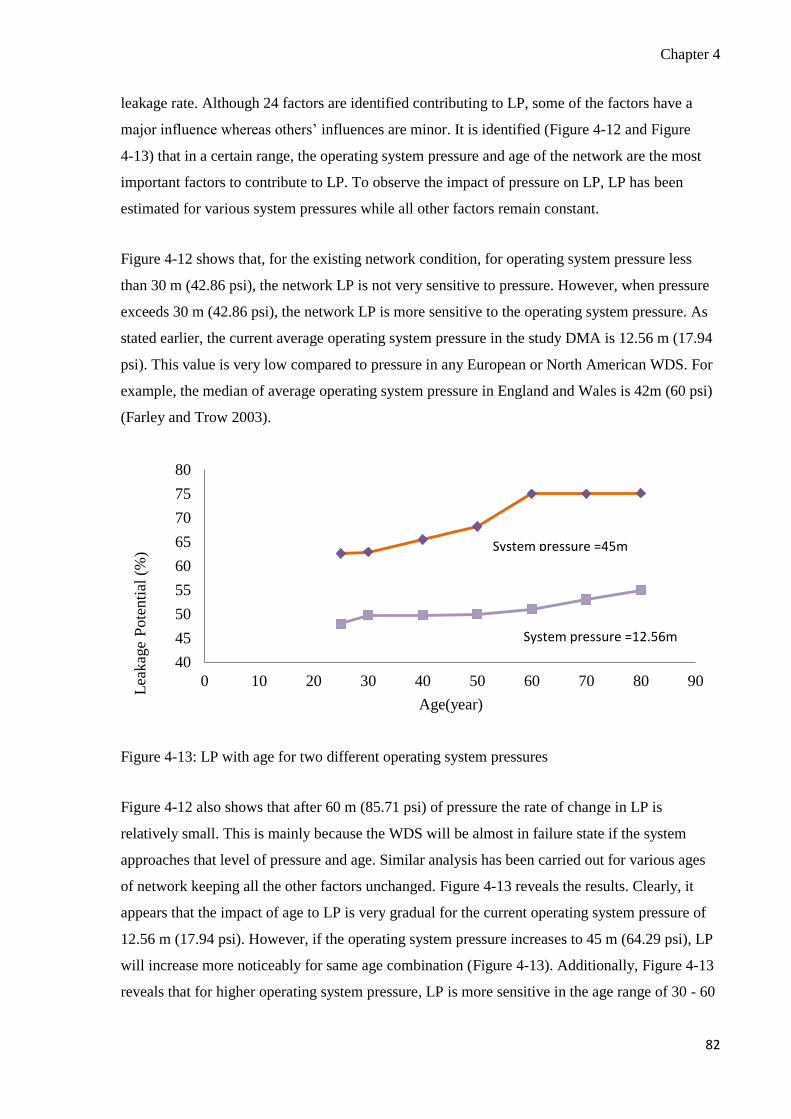
Chapter 4

82

leakage rate. Although 24 factors are identified contributing to LP, some of the factors have a

major influence whereas others’ influences are minor. It is identified (Figure 4-12 and Figure

4-13) that in a certain range, the operating system pressure and age of the network are the most

important factors to contribute to LP. To observe the impact of pressure on LP, LP has been

estimated for various system pressures while all other factors remain constant.

Figure 4-12 shows that, for the existing network condition, for operating system pressure less

than 30 m (42.86 psi), the network LP is not very sensitive to pressure. However, when pressure

exceeds 30 m (42.86 psi), the network LP is more sensitive to the operating system pressure. As

stated earlier, the current average operating system pressure in the study DMA is 12.56 m (17.94

psi). This value is very low compared to pressure in any European or North American WDS. For

example, the median of average operating system pressure in England and Wales is 42m (60 psi)

(Farley and Trow 2003).

Figure 4-13: LP with age for two different operating system pressures

Figure 4-12 also shows that after 60 m (85.71 psi) of pressure the rate of change in LP is

relatively small. This is mainly because the WDS will be almost in failure state if the system

approaches that level of pressure and age. Similar analysis has been carried out for various ages

of network keeping all the other factors unchanged. Figure 4-13 reveals the results. Clearly, it

appears that the impact of age to LP is very gradual for the current operating system pressure of

12.56 m (17.94 psi). However, if the operating system pressure increases to 45 m (64.29 psi), LP

will increase more noticeably for same age combination (Figure 4-13). Additionally, Figure 4-13

reveals that for higher operating system pressure, LP is more sensitive in the age range of 30 - 60

40

45

50

55

60

65

70

75

80

0 10 20 30 40 50 60 70 80 90

Lea

kag

e P

ote

nti

al (

%)

Age(year)

System pressure =45m

System pressure =12.56m

Chapter 4

83

years. This also indicates that the network will be virtually unusable after 60 years as the LP will

be very high.

Sensitivity Analysis 4.4.4

Uncertainties are inherently present in different influencing factors. To evaluate the impacts of

different uncertain parameters14, the research has applied Monte Carlo (MC) simulation

programmed in standard MATLAB coding environment, while the Spearman rank correlation

coefficients have been used to compare the impacts of different influencing factors.

As stated earlier, this research has identified a list of 24 leakage influencing factors for which

uncertainties has been modelled by assigning a probability distribution to each input

factor/parameter. The research applied a normal distribution for all basic factors. The means and

standard deviations of all parameters have been assumed based on estimated and/or observed

value. Due to lack of data, standard deviations for each factor has been assumed as 25% of the

mean as assumed for demand multipliers by Torres et al.( 2009).

The impacts of uncertainties of each factor/ parameter are related to the estimated values of

parameters or factors, not general for all ranges of values of parameters. The estimated factors

might be more or less sensitive in a certain range of their values. For example, LP is less sensitive

to an operating system pressure when it is less than 30 m (42.86 psi). The sensitivity becomes

more considerable when operating pressure is greater.

MC simulations generate multiple trial input values to estimate the value of random outputs. It

also predicts the error in the analysis which is inversely proportional to the number of iterations.

According to ProjectSmart (2010), total error in MC simulation can be estimated by:

[4-21]

where, σ is the standard deviation and N is the number of iterations. This equation has been used

to estimate the number of iterations for each MC simulation. Considering 1.5% error, the number

of trials has been calculated for the all 24 variables. The estimated maximum number of trials is

14

Modeled factors are termed as parameters. However, in some cases parameters and factors have been used

interchangeably.

Chapter 4

84

1600. However, for this study, 2000 iterations were carried out. Four scenarios (Table 4-4) have

been generated for the analysis.

Table 4-4: Definition of scenarios analyzed

Scenarios Variables Constant Parameters15 Special Treatment

Scenario I All except constant

parameters

RP,N1,SP, HL,PA,IA None

Scenario II All None None

Scenario III All None Mean operating system

pressure = 45 m

Scenario IV All None Mean operating system

pressure = 45m

Mean network age =35 years

Furthermore, in the sensitivity analysis, to compare parameter-wise influence to LP, Spearman

rank correlation coefficients were estimated. If ui is trial values of any input parameter and vi is

the corresponding LP values for those trial values, then the Spearman rank correlation coefficient

can be calculated by using Equation 4-22 (Walpole et al. 2007):

( )∑

[4-22]

where i =1, 2, 3 ... n; n is the number of pairs of data (number of iterations) and d is the difference

between the ranks of the ith value (ui) of input parameter and the corresponding LP value (vi).

4.4.4.1 Scenario I

As stated earlier, the most influencing factors for LP are pressure (e.g., reference system pressure,

pressure exponents, head loss and operating system pressure) and network age (e.g., age of the

pipe, age of the network instruments). To see the impacts of other factors, the sensitivity analysis

using MC simulation has been carried out.

Figure 4-14 presents (a) probability distribution function (PDF) and cumulative distribution

function (CDF); and (b) Spearman rank correlation coefficients. Figure 4-14 (a) shows that LP is

not very sensitive and most of the iterations calculated LP around 48%. Figure 4-14 (b) shows

that cover depth and traffic loading are the most influencing factors. It is industry practice to

respect a minimum cover depth of 1.2 m for a buried pipe.

15

See Table 3 for full name of abbreviate parameters

Chapter 4

85

Figure 4-14: MC simulation results for Scenario I (a) PDF and CDF (b) Spearman rank

correlation coefficients

46 47 48 49 50 51 52 530

0.1

0.2

Leakage potential(%)

PD

F v

alu

e

46 47 48 49 50 51 52 530

0.5

1

CD

F v

alu

e

0 2 4 6 8 10 12 14 16 18 20-0.8

-0.6

-0.4

-0.2

0

0.2

0.4

0.6

Parameter number

Rank c

orr

ela

tion c

oeff

icie

nt

(a)

(b)

Traffic loading Workmanship

Cover depth

Chapter 4

86

If this cover depth decreases while traffic loading and traffic flow increase, the risk of pipe failure

will increase significantly. Therefore, traffic loading is positively correlated whereas cover depth

is negatively correlated.

For the study network, the assumed mean cover depth and standard deviation is 0.6 m and 0.15

m, respectively. The small cover depth makes the network very vulnerable against traffic impact.

However, if the covered depth would have been more than 1.2 m then the cover depth and

loading would not be that sensitive. After the traffic factors, the workmanship parameters are the

next sensitive factors. This research studied four workmanships factors (e.g., pipe placement,

bedding backfilling, compaction and workmanship for network instruments).

4.4.4.2 Scenario II

Similar to Scenario I, for current operating condition a MC simulation has been carried out

considering all factors as variable. Both PDF and CDF, and the Spearman rank correlation

coefficients are presented in Figure 4-15. Figure 4-15 (a) shows that the shapes of PDF and CDF

have not changed significantly as compared to Scenario I in Figure 4-14 (a). However, an

additional peak is observed in PDF curve indicating less sensitivity of LP against the low

operating system pressure. However, the small gap (i.e., distance) between the two peaks on

Figure 4-15 (a) indicates less sensitivity of LP for this scenario. Nevertheless, the network might

behave quite differently if the operating system pressure increased to a range 30 – 60 meter

shown in Figure 4-12. These analyses have been conducted in Scenarios III and IV explained in

the next two sections.

Note that as Figure 4-12 indicates LP is not very sensitive to operating system pressure below 30

m. First small peak in Figure 4-15 (a) represents that less sensitive value. On the other hand,

Figure 4-13 suggests that at the age below 60 years for low pressure (e.g.,12.56 m or 17.94 psi)

and below 30 years for high pressure (e.g., 45 m or 64.29 psi), LP is not very sensitive to the age

of the network (i.e., the age of the pipes and age of the network appurtenances).

The estimated leakage potentials for these two cases are around 50% and 62%, respectively. The

second peak of Figure 4-15 (a) represents less sensitive value. The Spearman rank correlation

coefficients given on Figure 4-15 (b) reveal that the age of the pipe becomes more sensitive than

cover depth.

Chapter 4

87

Figure 4-15: MC simulation results for Scenario II (a) PDF and CDF (b) Spearman rank


42 44 46 48 50 52 54 56 580

0.05

0.1

0.15

0.2

0.25


PD

F v

alu

e

42 44 46 48 50 52 54 56 580

0.2

0.4

0.6

0.8

1

CD

F v

alu

e

0 5 10 15 20 25-0.8

-0.6

-0.4

-0.2

0

0.2

0.4

0.6

Parameter number

Rank c

orr

ela

tion c

oeff

icie

nt

CDF

(a) PDF

Traffic loading

Cover depth

Pipe age

(b)

Chapter 4

88

This study assumed the mean and standard deviation of the age of the network are 25 years and

6.25 years, respectively. In addition to the impact of the network age, the cover depth and traffic

loading are the most critical influential factors.

4.4.4.3 Scenario III

In this scenario, MC simulation has been carried out considering all parameters as variable for the

current operating condition. However, operating system pressure has been changed to 45 m

(64.29 psi). This pressure has been selected from the sensitive region of Figure 4-12. Figure 4-16

shows the results for (a) PDF and CDF and (b) Spearman rank correlation coefficients. Though

Figure 4-15 (Scenario II) and Figure 4-16 (Scenario III) show nearly similar shape of the PDF,

Figure 4-16 represents a wide range of LP. This wide range indicates that with increase of

pressure, influences of all other factors change significantly. The point of inflection in the CDF

curve represents the second peak of PDF. Therefore, the point of inflection in the CDF curve

indicates less sensitivity of LP for parameters at that point.

From Figure 4-16 (b), it is evident that the system pressure and pressure related factors become

the main drivers. The most influencing factors are system pressure, pressure exponent, reference

system pressure, age of the network and cover depth. It is important to note that reference system

pressure is negatively correlated with LP which means with the decrease of reference system

pressure, LP will increase for the same system operating pressure.

4.4.4.4 Scenario IV

This scenario is identical to Scenario III except that the age of the network has been increased to

35 years. Similar to previous three scenarios, Figure 4-17 shows (a) PDF and CDF and (b)

Spearman rank correlation coefficients. The difference in two peaks of Figure 4-15 (Scenario II)

and Figure 4-16 (Scenario III) become less noticeable. Therefore, the point of inflection in the

CDF is less visible. It is also observed that due to increase of age, the value of PDF has increased

towards the highest range of LP.

This indicates that if the network age is around 35 years and operating system pressure is 45m,

the network will be virtually unable to deliver water to the customers. Like scenario III, Figure

4-17 (b) reveals that operating system pressure and pressure related factors are the most

influencing factors followed by the age of the pipe.

Chapter 4

89

Figure 4-16: MC simulation results for Scenario III (a) PDF and CDF (b) Spearman rank


40 50 60 70 80 90 1000

0.01

0.02

0.03

0.04

0.05


PD

F v

alu

e

40 50 60 70 80 90 1000

0.2

0.4

0.6

0.8

1

CD

F v

alu

e

0 5 10 15 20 25-0.4

-0.2

0

0.2

0.4

0.6

0.8

1

Parameter number

Rank c

orr

ela

tion c

oeff

icie

nt

CDF

PDF

(a)

(b)

Cover depth

Pressure exponent

System pressure

Pipe age

Reference

pressure

Chapter 4

90

Figure 4-17: MC simulation results for Scenario IV (a) PDF and CDF (b) Spearman rank


40 50 60 70 80 90 1000

0.02

0.04


PD

F v

alu

e

40 50 60 70 80 90 1000

0.5

1

CD

F v

alu

e

0 5 10 15 20 25-0.3

-0.2

-0.1

0

0.1

0.2

0.3

0.4

0.5

0.6

0.7

Parameter number

Rank c

orr

ela

tion c

oeff

icie

nt

14(b)

(b)

Cover depth

Reference system

ressure

Pressure exponent

System pressure

Pipe age

(a)

CDF

PDF

Chapter 4

91

4.5 Model Summary

This part of the research developed a FRB model to estimate LP for WDS identifying various key

leakage influencing factors. A normalization method has been adopted which will simplify the

interpretation of the FRB modelling results to the non-technical people. Additionally, a new

adjusted FRB methodology has been proposed to adjust the impact of such factors which can also

influence other contributory factors.

Detailed sensitivity analysis revealed that the operating system pressure and pressure related

factors such as reference system pressure and pressure exponent are the most influencing factors.

The results also confirmed that after pressure related factors the pipe age are the most important

factor. However, the sensitivity of these factors varied according to the range of operating system

pressure and network age. It is also identified that cover depth of the pipe is very influential in a

certain range. However, cover depth is less pressure dependent. The next influencing factors are

different kinds of workmanship of the network and network appurtenances. It is noted that among

twenty four factors around half (e.g., pressure related factors, age, workmanships, cover depth) of

them are the most influential on the LP and the remaining half of the factors (e.g., ground water

table fluctuation, head loss, soil type) have minimal influences.

Though this model has been applied to a network of low pressure, the model can be used for any

network by modifying appropriate factors/parameters. Indeed, the model should be updated based

on any specific condition of any particular network, especially ranges of different influencing

factors. Moreover, the developed methodology can be extended for other cases for similar

problem. For the case study, some of the data have been estimated based on the information

collected from state-of-the practice, manuals and the experiences in the study area. However, by

collecting these data, estimated LP would be more accurate. Like almost all risk-based modelling

approaches, this study also suffers from lack of validation data. In spite of the limitation, the

proposed methodology is capable of helping water utility managers to prioritize their leakage

control and rehabilitation policy through better understanding of their network.

In future studies, the developed model could be linked with US EPA developed EPANET model

as an add-on. That will give the capability to EPANET to calculate LP for pipes and to map the

spatial distribution of LP within WDS.

Chapter 5

92

CHAPTER 5 LEAKAGE DETECTION AND LOCATION MODEL

An version of this chapter has been published in Urban Water Journal [8(6), 351–365] with the

title “Leakage Detection and Location in Water Distribution System Using a Fuzzy-Based

Methodology” (Islam et al. 2011b).

5.1 Introduction

As stated earlier, leakage from a WDS is a universal problem. There is no single reason for the

occurrence of leakage in any WDS. There are numerous physical, environmental, and hydraulic

factors that pose threats to make WDSs vulnerable to leakage. Whatever the reasons might be, if

the leakage is identified, and controlled in a minimal time after its occurrence, a significant

volume of treated water can be saved.

From the time of occurrence of WDS’s leakage, to its return to a normal operating condition, the

time can be divided into three stages (ALR): (a) leakage awareness time, (b) leakage location

time, and (c) leakage repair time. Awareness time is the time required for a utility organization to

be aware of the existence of leakage in a system. The location time is the time required for a

utility to locate the leakage after being made aware of its existence, and the repair time is the

actual time required for repairing the leakage (Farley and Trow 2003). After an occurrence of

leakage, if these three times (ALR) are minimal, then the water lost through leakage from the

system will be minimal. However, the ALR time required for a system depends on leakage

detection processes, best management practices, technologies, the number and the skill of the

staff involved, and overall, most importantly, an active leakage control (ALC) policy of the

utility. For example, a WDS with regular sounding16 once per year, the average duration for

awareness and locating for a leakage in a service pipe or main would be 183 days (Lambert

1994). On the other hand, if a utility checks for leakage on a daily basis, the awareness and the

16

A systematic survey technique for listening for leak noises on hydrants, valves, stop taps or at the ground

surface above the line of the pipe line. Various types of equipment are available; however, the sounding stick is

a basic one, which can be used as a simple acoustic instrument or an electrically amplified instrument (Farley

and Trow 2003).

Chapter 5

93

leakage location time will be significantly lower. Table 5-1 compares average running times for

an unreported burst under different WDS monitoring conditions, where an unreported burst refers

to the burst that runs until identified by an active leakage control action (Lambert 1994). It is

obvious that a fast detection can save awareness time significantly, which eventually save a large

volume of water leaking from a WDS.

Over the last hundred years, water utilities have been using different techniques, including

manual sounding, acoustic loggers, ground-penetrating radars, helical vane meters, deacon

meters, leak noise correlators, step testing, combined acoustic loggers and correlators, electronic

step testers, digital correlators, advanced ground microphones, and so forth to detect leakage in

their systems (Pilcher 2003). In recent times, the real time monitoring of WDS using different

sensors has been used to detect anomalies in water distribution systems. Water utilities have been

adapting real time monitoring techniques, coupled with burst and background estimate (BABE)–a

component-based leakage volume estimation (Lambert 1994) technique to estimate the leakage in

WDS. But, generally, the real time monitoring is not enough to detect the leakage. Information

needs to be extracted by analyzing the monitored data to detect leakage. An efficient detection

and diagnosis algorithm is prerequisite to identify leakage in a WDS. There have been many

studies conducted to increase the efficiency and the confidence of the detection and diagnosis

algorithms. A summary of some of the important studies relevant to this research has been

reported in literature review chapter. Each of the reported algorithms and formulations has some

noted advantages but also suffers constraints. There are many other related studies (e.g., Covas et

al. 2005; Webb et al. 2009) that highlight the importance of continuing research for leakage

detection and diagnosis.

Table 5-1: Importance of time and technology in leakage (Modified from Lambert 1994)

WDS Type Leakage control policy Average running duration (days)

Awareness Location Repair

Non-metered WDS

Sounding once in two years 365

1 to 2

days*

Between 4

to 10 days*

Sounding once in one year 183

Sounding twice in one year 93

Metered WDS Monthly meter reading 15

Metered WDS with

data logger Weekly data download 3 to 4

No-metered WDS

with telemetry Continuous <1

*Highly depended on employed technology and also number, capabilities and efficiency of the

leak location and repair staff.

Chapter 5

94

Generally, the literature on leakage detection and diagnosis acknowledge high levels of

uncertainties. However, most of them did not incorporate the uncertainties related to the different

WDS parameters in their algorithms, and even when incorporated, it was poorly addressed.

Therefore, the reported algorithms may either produce many costs-incurring false positive alarms

or fail to detect real leakage events by generating false negative alarms.

A WDS is a distributed system consisting of a set of links and nodes. The physical junctions of

the pipes, points of any changes in linear pipes, reservoirs, and tanks are generally known as

nodes, whereas all the pipes, valves, and pumps are considered links. Due to the continuous

changes in friction coefficients, nodal demands, and reservoir water levels, it is very difficult to

predict those parameters. Because of the semi-quantitative nature of the independent parameters,

the simulated WDS dependent parameters (i.e., pressures at nodes and flow in pipes) are

subjected to uncertainties.

Using fuzzy-based algorithms, Revelli and Ridolfi (2002) proposed an optimization-based

methodology in order to address this issue by calculating the extreme values (i.e., maximum and

minimum) of the WDS dependent parameters. Gupta and Bhave (2007) developed a methodology

to incorporate the parameter uncertainties using a fuzzy-based approach. To obtain the same

solution for the WDS used by Revelli and Ridolfi (2002), the algorithm developed by Gupta and

Bhave (2007) , however, requires less computational efforts. Using normal values of the

independent parameters (e.g., roughness coefficients, nodal demands, reservoir water levels, and

so forth), the normal values of the dependent parameters, such as pressure, quality, and age, of

water for all nodes, and flow, velocity, and quality of water within all pipes, were simulated.

However, the maximum and the minimum values of independent parameters did not produce the

maximum and the minimum values of the dependent parameters, respectively. This study showed

that some combinations of maximum and minimum values of the independent parameters may

produce extreme values of the dependent parameters (Gupta and Bhave 2007).

Fuzzy sets are used to deal with vague and imprecise information (Zadeh 1965). Instead of

providing any information with crisp value, fuzzy sets model the information with a degree of

membership where the most likely value has a full degree of membership, and the least likely

values have the zero membership. Fuzzy set theory is widely applied to solve real-life problems

that are subjective, vague, and imprecise in nature (Smithson and Verkuilen 2006; Yang and Xu

2002). Since its conceptualization, fuzzy set theory has been used in various engineering

applications, including civil and water engineering. It is successfully implemented for structural

Chapter 5

95

damage analysis, vibration control of flexible structures, cement rotary kiln control, and concrete

analysis and design (Gad and Farooq 2001). Sadiq et al. (2007) implemented fuzzy sets for

predicting water quality failures in WDS. There are numerous other examples for the application

of fuzzy sets in water distribution modelling.

5.2 Leakage Detection and Location Model Development Methodology

This section of this research proposes a novel methodology to detect the presence of leakage, and

highlights the most likely leakage location in the WDS. To better address the uncertainties in the

proposed leakage detection and diagnosis methodology, the uncertainties of different independent

parameters are described using fuzzy sets. Fuzzy set theory has been used for modelling complex

systems, and handles uncertain and imprecise information effectively (Ross 2004). In this study,

the algorithm developed by Gupta and Bhave (2007) has been adopted to simulate the maximum

and the minimum values of the dependent parameters for extended period of simulation.

Monitored pressures in different nodes and flows in different pipes are used to estimate the

degrees of memberships of leakage and its severity in terms of index17 of leakage propensities

(ILPs). The ILPs help to identify the most likely leakage location in a WDS.

The proposed methodology requires the identification and fuzzification of different independent

parameters such as roughness coefficients, nodal demands, and water reservoir levels, as well as

three sets of WDS solutions. As reported in previous studies (Gupta and Bhave 2007; Revelli and

Ridolfi 2002), it is assumed that the independent parameters are triangular fuzzy numbers. Three

sets of WDS solutions include one set for a normal WDS condition to represent the most likely

values, and two sets for the maximum and the minimum values of the dependent parameters (e.g.,

pressure in all nodes and flow in all pipes). The solution for a normal condition of a calibrated

model estimates the values of dependent parameters (for all nodes and links), whereas the other

two sets estimate the two extreme sets (i.e., maximum and minimum) of the possible values of

dependent parameters (for all nodes and links). Details of the adopted methodology have been

provided in Section 5.2.2. It is noted that the accuracy of the leakage detection depends on the

well-calibrated model. However, in practice, the standard of hydraulic model calibration is not

often pleasing. In such a situation, detection and location of a small leakage will be error-prone.

17

It is a ratio of deviation of the monitored flow from the most likely value to deviation of the extreme value

from the most likely value. Details have been discussed in Section 5.2.4.

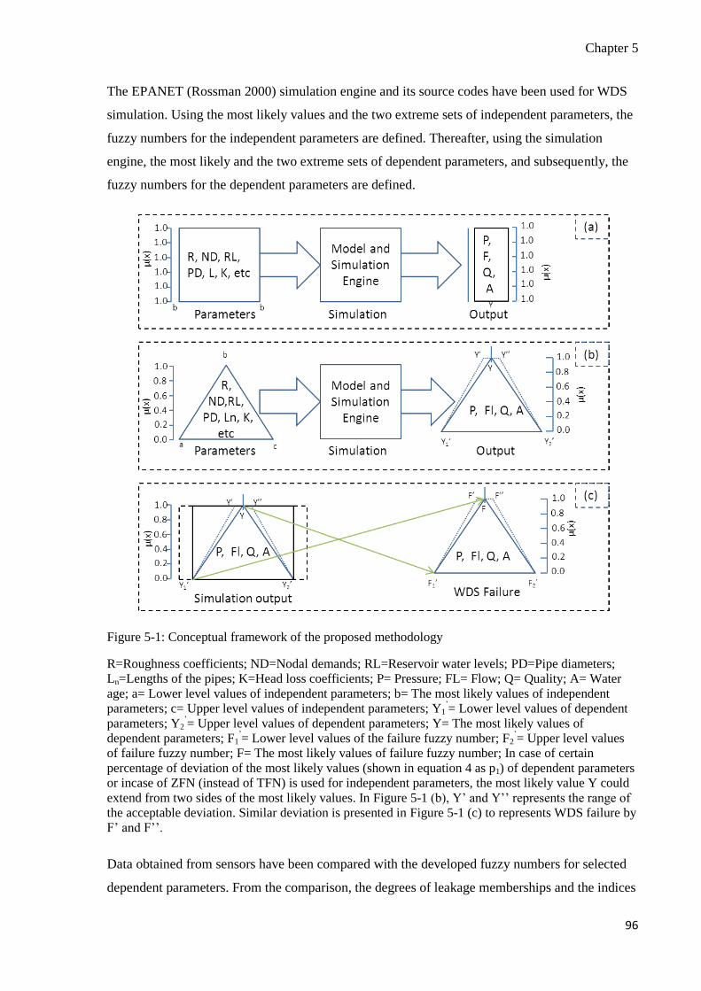
Chapter 5

96

The EPANET (Rossman 2000) simulation engine and its source codes have been used for WDS

simulation. Using the most likely values and the two extreme sets of independent parameters, the

fuzzy numbers for the independent parameters are defined. Thereafter, using the simulation

engine, the most likely and the two extreme sets of dependent parameters, and subsequently, the

fuzzy numbers for the dependent parameters are defined.

Figure 5-1: Conceptual framework of the proposed methodology

R=Roughness coefficients; ND=Nodal demands; RL=Reservoir water levels; PD=Pipe diameters;

Ln=Lengths of the pipes; K=Head loss coefficients; P= Pressure; FL= Flow; Q= Quality; A= Water

age; a= Lower level values of independent parameters; b= The most likely values of independent

parameters; c= Upper level values of independent parameters; Y1’= Lower level values of dependent

parameters; Y2’= Upper level values of dependent parameters; Y= The most likely values of

dependent parameters; F1’= Lower level values of the failure fuzzy number; F2

’= Upper level values

of failure fuzzy number; F= The most likely values of failure fuzzy number; In case of certain

percentage of deviation of the most likely values (shown in equation 4 as p1) of dependent parameters

or incase of ZFN (instead of TFN) is used for independent parameters, the most likely value Y could

extend from two sides of the most likely values. In Figure 5-1 (b), Y’ and Y’’ represents the range of

the acceptable deviation. Similar deviation is presented in Figure 5-1 (c) to represents WDS failure by

F’ and F’’.

Data obtained from sensors have been compared with the developed fuzzy numbers for selected

dependent parameters. From the comparison, the degrees of leakage memberships and the indices

Chapter 5

97

of leakage propensity (ILPs) have been estimated for pipes and nodes. If a sensor data is same as

the most likely value then the degree of leakage membership is zero, and if the sensor data is the

same as the lowest value, then the degree of leakage membership is one. However, if the sensor

data is higher than the most likely value it will not represent the leakage; it will indicate another

form of anomaly such as blockage. The latter is not addressed in this study.

Figure 5-1 provides the conceptual framework for the proposed methodology. Details of the

algorithm are discussed in Sections 5.2.3 and 5.2.4. Different stages of the proposed methodology

and the EPANET toolkits’ functions have been implemented using MATLAB 7.10 (MathWorks

2010).

In Figure 5-1 (a), all the independent and the calculated dependent parameters are deterministic.

Therefore, they have a full degree of membership of their values. However, in Figure 5-1 (b), all

the independent and the dependent parameters are fuzzy and they have different degrees of

membership of their values. In Figure 5-1 (c), the simulated most likely dependent parameters

indicate no failure whereas any deviation from the most likely value indicates the presence of

anomalies. The deviation up to their two extreme values indicates the full membership of their

failure.

Identification and Fuzzification of Independent Parameters 5.2.1

Water distribution systems are complex infrastructure. Modelling of such an infrastructure

involves many parameters, such as diameters, lengths and roughness coefficients of pipes, nodal

demands, water levels in reservoirs and head-discharge characteristics of pumps, and

performance characteristics of different valves and minor elements (Gupta and Bhave 2007).

Among those parameters some are very precise, such as pipe lengths, some are imprecise such as

roughness coefficients, and some are in between, such as nodal demand, for which a statistical

distribution can be generated if enough information is available (Revelli and Ridolfi 2002).

On the other hand, some of those imprecise parameters may a have significant impact on WDS,

whereas some may have a low impact. Therefore, the parameters which are relatively imprecise,

and have significant impact on the WDS simulation results have been selected for fuzzification.

However, inclusion of all WDS independent parameters for fuzzification will not reduce the

reliability of the results, but, will reduce the computational efficiency. Roughness coefficients,

nodal demands, and reservoir water levels are considered the most common parameters which are

Chapter 5

98

imprecise and may have a significant impact on results (Gupta and Bhave 2007; Revelli and

Ridolfi 2002).

After the selection of independent parameters, the most likely and the extreme values of the

selected parameters are defined. The values of independent parameters of a calibrated model can

be used as the best estimate for the normal values, whereas the extreme values can be estimated

based on reported literature values, industry practice experiences, and other supporting data or

certain percentage of the normal values, defined based on experts’ judgement. In Figure 5-1, the

normal values of the independent parameters are represented by b whereas a and c represent the

minimum and the maximum values, respectively (which can also be seen in Figure 5-2). Based

on the minimum, the most likely and the maximum values of all the selected independent

parameters, fuzzification has been carried out. To fuzzify the data, generally triangular fuzzy

numbers (TFN) or trapezoidal fuzzy numbers (ZFN) are used (Lee 1996). All the selected

parameters (e.g., roughness coefficients, nodal demands, reservoir water levels, head loss

coefficients, and so forth) have been fuzzified (Figure 3-4). As described in Chapter 3, Equations

3.2 and 3.3 (Chapter 3) have been used to model the TFN and ZFN. For a TFN, a is the minimum

value, b is the most likely value and c is the maximum value of an independent parameters. For a

ZFN, a is the minimum value, d is the maximum value and b and c are the two values which

represent the interval of the most likely value. We assume that the fuzzified values of

independent parameters are in an Nx3 matrix [a b c], where N is number of an independent

parameter.

Although the fuzzy independent parameters are strictly triangular or trapezoidal with linear sides

(e.g., ab’ and b’c for TFN and ab’ and c’d for ZFN), the corresponding fuzzy numbers for

dependent parameters will be also triangular or trapezoidal but with curvilinear sides (e.g., ab’

and b’c for TFN and ab’ and c’d for ZFN) (See Figure 3-4), because of the nonlinearity of the

system (Revelli and Ridolfi 2002). However, the difference between the linear and the curvilinear

sides is small (Gupta and Bhave 2007). Therefore, the fuzzy numbers for dependent parameters

have been considered triangular or trapezoidal with linear sides.

Estimation of Extreme Values of Dependent Parameters 5.2.2

Following the steps described in section 3.2.2 in Chapter 3 , the extreme values of hydraulic

dependents parameters are estimated. Based on the steps described in section 3.2.2 in Chapter 3,

Chapter 5

99

the fuzzy values of the dependent parameters for 24 hours can be estimated. Figure 5-2 shows the

flowchart showing the different steps of the proposed algorithm.

Identify independent

parameters to be

fuzzified

for a time step

Estimate normal values

of selected

independent

parameters [b]

Fuzzify independent

parameter

[a b c]

Calibrated model

Simulation engine

For normal condition,

estimate desired

dependent parameters

[Y]

Change an

independent parameter

to its maximum value

Estimate desired

dependent parameters

[Dn]

Calculate

C=[Dn-Y]

If C>0 then Mx=c

If C<0 then Mx=a

If C=0 then Mx=b

Literature review

If C<0 then My=c

If C>0 then My=a

If C=0 then My=b

For minimum dependent

parameters calculation

Fo

r m

axi

mu

m d

ep

en

de

nt

pa

ram

ete

rs c

alc

ula

tion

Max. dependent

parameters (Y’2)

Simulation

for independent minimum

parameters completed?

Min. dependent

parameters (Y’1)

Fuzzy

dependent

parameters

Simulation

engine

YesNONO

Have we finished

for all time

steps?YES

NO

End

Reinstate to normal

condition

Simulation

for independent maximum

parameters completed?

Reinstate to

normal condition

Figure 5-2: Flowchart for proposed methodology

Chapter 5

100

Leakage Detection 5.2.3

This part of the algorithm has been developed based on the simulation results of an undamaged

WDS. Under the assumption that M is a calibrated hydraulic model with an array of independent

parameters, X =[

]

where i represents different kind of the independent parameters such as the roughness

coefficients, nodal demands, reservoir water levels, pipe diameters, pipe lengths, head loss

coefficients, and so forth and j is the number of each i. For example, if i is the roughness

coefficients then j is the number of pipes, and if i is the nodal demands, then j is the number of

nodes. The simulation of a calibrated hydraulic model M (b) estimates an array of dependent

parameters, Y=[

]

where r is the number of dependent parameters such as pressure, flow, quality and j is the number

of each r. Using the algorithm presented in Section 5.2.2, the WDS has been solved for the two

extreme solutions. We assume, the extreme solutions of the WDS is (Y’12), where Y’12 represents

both the minimum (Y’1) and the maximum (Y’2) solutions of all the dependent parameters. The

monitored/ sensor data will be evaluated with respect to the fuzzy numbers defined from these

three sets of solutions (Y, Y’1 and Y’2). Assume Ŷ is an array of monitored / sensor data for a

particular time, expressed as Ŷ =[

]

where m refers to different monitored parameters such as flow, pressure, quality and k is the

number of each m. If all the dependent parameters are monitored then m and r will be the same

number and if the monitored data are available for all nodes and pipes, then k and j will have the

same number. In case of leakage detection, flow and pressure are considered as dependent

parameters; therefore, m = 2 and k = number of the monitoring locations at a particular time.

After the selection of key parameters, the system will calculate the departures of the monitored

values from the accepted ((Yij)*p1) values (Equation5-1).

Dkm(X) = (Ykm)*(±p1)–(Ŷkm) [5-1]

Chapter 5

101

where, p1 is the deviation factor. If no deviation of the calibrated values from the normal values is

expected, then p1 is considered as 1, provided that the defined independent fuzzy numbers are

triangular. However, if a deviation of the calibrated values from the normal values is acceptable

then p1 could have a different value (based on the acceptable deviation). We assume a situation

where the calibrated model can estimate correct pressure and flow, and represents the most likely

value. In Figure 5-3, the Y represents the most likely value and acceptable value of pressure and

flow.

Figure 5-3: Leakage detection algorithm

If the monitored sensor pressure is in the range of acceptable values then no failure (either

leakage or blockage) is considered. If the monitored pressure is less than the most likely value

then the system anomaly is due to a leakage or an unusual demand in the system. However, if the

monitored pressure is higher than the most likely value, then the anomaly is due to a blockage. If

there is an unusual demand, it will not continue for long time, however, in case of leakage, it will

continue until it is controlled. If the demand variation is due to another reason (e.g., repair or

rezoning), the model can also detect that variation, however, the decision makers need to decide

how to treat the detected variation. For a weekend demand variation, it is necessary to use a

model calibrated for the weekend.

In general, the monitored values will have certain extent of deviations due to various

uncertainties. These deviations can go up to the estimated two extreme values. If a monitored

value of a sensor goes to any of the two extreme values or beyond then the anomaly in a system

is assigned a full membership. In a normal operating condition, going to such extreme values is

very unlikely. If a monitored value of a sensor is in between the extreme values then the system

will treat it as a failure with a certain degree of failure membership. The degree of failure

membership for each monitored parameter will be estimated as follows:

Chapter 5

102

{

[5-2]

where, Rf is the degree of failure membership; Ŷ represents monitored data for a particular time

and Y’12 represents both the minimum (Y’1) and the maximum (Y’2) values of the dependent

variable. As both the minimum and maximum values are not possible to happen simultaneously,

therefore, Y’12 should be replaced with (Y’1) in case of minimum or (Y’2) in case of maximum. In

addition, in the normal acceptable condition, the calculated degree of failure membership will be

relatively smaller than their value in a failure condition. Therefore, increase in the values of

degrees of failure memberships at different nodes / pipes from their values in normal condition

will point out an anomaly in the system.

Node and Pipe Identification 5.2.4

Occurrence, in terms of location and amount, of leakage in a system is random. Due to leakage

any monitored value could go beyond the two extreme values. To address this issue, coupled with

the degree of leakage (failure membership), the index of leakage propensity (ILP) has been

proposed. If a monitored value is within the range of the extreme values (inclusive) then the ILP

is the same as the degree of leakage. However, if a monitored value is beyond the extreme values

then the ILP is more than unity. The concept of ILP has been used to highlight the most likely

leaky node as well as the most likely leaky pipe.

Leakage is pressure dependent demand (Lambert 2001). The presence of leakage in a node/ pipe

not only changes the flow and pressure in the leaky node / pipe, and the downstream part of the

WDS, it also changes the flow and pressure in the whole WDS to a certain extent. However, after

the most significant impacts on leaky node, the 2nd most, the 3rd most and so forth, impacts will

be observed on the adjacent 2nd, 3rd and so forth, nodes/ pipes of the leaky node, respectively.

If the leakage is large enough and located near the sensor location, the deviation of the monitored

flow / pressure from the normal flow / pressure could go beyond the possible extreme values, and

therefore, the ILP could be more than 1 in multiple nodes or pipes. However, the ILP will be the

highest at the leaky node/ pipe. Therefore, the leaky node/pipe will be the one which has the

highest ILP over the time after leakage. To ensure the leaky node or the leaky pipe is well

identified, it is expected that the node with the second highest ILP / degree of leakage will be

adjacent to the highest one. Therefore, after the identification of the leaky node/pipe, all the

Chapter 5

103

nodes/ pipes have been ranked based on their ILPs. In the case of pipes, it is expected that the

identified most likely leaky pipe will be connected to the identified most likely leaky node. For

example, in the case of a leaky node with four connected pipes, the 1st, 2nd, 3rd, and the 4th most

likely leaky pipes will be connected to that node. From this topological information, the most

likely leaky node and the most likely leaky pipe can be identified.

Installing pressure and flow sensors in all the key nodes is unlikely. In reality, in most WDSs, the

numbers of the sensors are much lower than the number of nodes. In such situation, the above

methodology could identify the presence of the leakage and the nearest sensor to the leakage. To

highlight the nearest leaky node or pipe, additional investigation need to be carried out. For this

case, an optimum number of sensors need to be installed in the WDS. This optimum number of

sensors depends on the size of the WDS and the sizes of the leakage (leakage flow) to be

detected. The number of the sensors should be such that the presence of the leakage must

influence at least one sensor, and in the reverse way, the methodology will be able to detect only

that size of leakage (or higher) which will be able to influence at least one sensor. In a DMA

(district meter area) structured system, if there is only one flow and pressure meter at the DMA

inlet, then this methodology can not detect the leaking node. However, if the leakage search is

conducted over the whole WDS (composed of multiple DMAs), then the algorithm can find out

the leaky DMA. As a part of additional investigation, for a single leakage, an emitter has been

modelled based on the assumed emitter coefficient and pressure exponent.

An Emitter is a device associated with junctions that model the flow through a nozzle or an

orifice that discharges to the atmosphere (Rossman 2000). It can model the pressure depended

demand (e.g., leakage) as an emitter flow in the form of Equation 5-3 (Wu et al. 2010).

ql,i(t) = Ci [pi(t)]N1 [5-3]

where ql,i(t)is the leakage flow rate at node i at time t, Ci is the discharge coefficient at node i,

pi(t) is the nodal pressure at node i at time t and N1 is the emitter exponent or pressure exponent .

The values of pressure exponent generally varies in between 0.50 and 2.50, depending upon the

type of leakage paths, network ages, corrosion types, pipe material and other network related

factors (Farley and Trow 2003). A positive value of emitter coefficient will result in a leakage

demand.

Chapter 5

104

As discussed before, the presence of leakage will be identified based on the estimated degrees of

leakage and the ILPs at sensor locations. To do that, the WDS with the normal values of

independent parameters need to be solved putting an emitter coefficient in a node. This procedure

needs to be repeated by putting the same emitter coefficient in all nodes. During each solution,

the ILPs at sensor locations need to be estimated and compared (in terms of deviation) with the

ILPs calculated when the first anomaly was detected. The absolute deviation of the ILPs at sensor

locations will be minimal when the ILPs have been estimated from the network solution putting

the emitter coefficient at the leaky node. The same comparison need to be carried out for all the

sensors which can identify the presence of leakage. If the number of leakages in the system is

more than one then the WDS needs to be analysed for the combination of multiple emitter

exponents and nodes. However, the required calculations will be minimal if the most likely leaky

area is identified from the available sensor data. In that case, the network solutions, assigning

emitter coefficients to nodes, will be required only on the nodes in the identified most likely

leaky area and, hence, the computational efforts will be less. In a similar way, the most likely

leaky pipe also needs to be identified. Based on the most likely leaky node and pipe information,

the final leaky node/pipe will be identified.

5.3 Model Implementation

To demonstrate the applicability of the leakage detection and location methodology, the

developed model based on the proposed methodology has been implemented and demonstrated

through the example WDS used in section 3.3 in Chapter 3. The example WDS has 40 pipes with

a total length of 19.5 km, connected by 27 nodes. Water is supplied by gravity from the two

elevated reservoirs (reservoir 1 and reservoir 2) with the total head of 90 m, and 85 m,

respectively. The lengths of the pipes vary from 100 m to 680 m, and the diameters of the pipes

vary from 200 mm to 700 mm. Base demands at different nodes varies from 50 l/s to 100 l/s and

demand multipliers ranges from 0.38 at 5am to 1.46 at 9 am. Detail information on pipe length,

diameter, roughness coefficient, nodal connectivity, and nodal hourly base demand and demand

multipliers and two reservoirs head have been provided in Table 3-6 in Chapter 3.

The WDS has been considered as an undamaged system, and all the parameter values are

considered as calibrated values in normal condition. The parameters such as roughness

coefficients, nodal demands, reservoir water levels, pipe diameters, length of the pipes, and head

loss coefficients are uncertain. For this case study, only the roughness coefficients, nodal

demands and the reservoir water levels have been taken as uncertain independent parameters.

Chapter 5

105

According to the procedure described in Section 5.2.1, the minimum, the most likely and the

maximum values of the independent parameters are selected. As assumed by Gupta and Bhave

(2007), for the reservoir levels ±0.5 m, for the roughness coefficients ±5, and for the nodal base

demands ± 5% deviations from their normal values have been considered to estimate the two

extreme values of those independent parameters. Coupling the procedure described in Section

5.2.2 with EPANET determines minimum, most likely and the maximum values of dependent

parameters at all nodes and pipes over a period of 24 hours.

Based on the estimated normal, minimum and maximum values of the dependent parameters, a

set of fuzzy numbers has been derived for all nodes and pipes over the period of 24 hours.

Artificially created pressure and flow sensor data are fed into the developed model to diagnose

any anomalies (e.g., the leakage) in the WDS.

Leakage Data Preparation 5.3.1

As the study has been carried out on an example WDS, the sensor data or monitored data are

prepared by simulating the WDS under a leaky condition. To represent the leakage in a WDS, an

emitter coefficient and a pressure exponent has been incorporated at a node of the calibrated

hydraulic model. To represent randomness (both in terms of size and location) in the leakage an

arbitrary emitter coefficient of 0.95 and a pressure exponent of 1.10 have been randomly

incorporated into node 20. Although, the emitter coefficient is completely random, the value of

pressure exponent N1 (1.1) has been selected to represent a medium aged network. It is noted that

the value of pressure exponent of a network can be estimated from a standard pressure step test (a

standard test carried out at the time of minimum night flow to estimate the leakage).

The emitter generates pressure dependent leakage demand to node 20 which is in addition to the

base demand. After the incorporation of leakage demand, the WDS has been solved for the

normal operating condition. The solutions for different nodes and pipes for this WDS represents

monitored/ sensor data for all nodes and pipes under the leaky condition due to leakage at node

20).

In the case of limited number of sensors, arbitrarily five pressure sensors have been placed at the

nodes no. 4, 7, 9, 17, and 19 so that those sensors can cover the whole WDS. Although, in this

study, the number of sensors and their placement locations has not been optimized, it would be

preferable to find the optimal number of sensors and their locations in the WDS. To represent the

Chapter 5

106

leaky condition of the WDS, the emitter coefficient has been applied arbitrarily to node no. 13.

The WDS has been simulated in the normal condition, and the simulated node and pipe results for

nodes no. 4, 7, 9, 17, and 19 represent the pressure sensor data for those nodes.

Leakage Detection 5.3.2

After estimating the degrees of leakage and the ILPs, it is observed (Table 5-2) that, in certain

times of the day, node 25 has a degree of leakage of 1 and the ILPs higher than 1 which indicate

the presence of anomaly in the WDS. However, if the leakage to be detected has little flow rate,

no ILP will be higher than 1. In that case, the presence of leakage can be identified from the

maximum value of the degrees of leakage / ILPs and their deviations from their normal values.

On the other hand, if the leakage is large, it is anticipated that more than one node could have

ILPs greater than 1. In that case, the most likely location of the leakage will correspond to the

maximum ILP location. As an example, Table 5-2 shows the degree of leakage and the ILPs in

node 13 and node 25 over 24 hours of a typical day.

Table 5-2: Typical degrees of leakage memberships and the associated ILPs

Time

(hour)

Node 13 Node 25

µ(x) ILP(x) µ(x) ILP(x)

0-2 0.96 0.96 1.00 3.06

2-4 1.00 1.07 1.00 5.57

4-6 1.00 1.05 1.00 5.77

6-8 0.86 0.86 1.00 2.21

8-10 0.27 0.27 0.59 0.59

10-12 0.31 0.31 0.69 0.69

12-14 0.67 0.67 1.00 1.70

14-16 0.76 0.76 1.00 2.05

16-18 0.50 0.50 1.00 1.19

18-20 0.23 0.23 0.49 0.49

20-22 0.47 0.47 1.00 1.10

22-24 0.61 0.61 1.00 1.52

If the changes in the flow or pressure are only due to the variation of base water demand or

changes in other independent parameters, then the degree of leakage and the ILPs will be 1 or

less, as the values of the independent parameters can not go beyond their extreme values. In a

rare case, if any high abnormal demand like fire flow exists in the system, it is unlikely to

continue for a whole day or longer. From Table 5-2, it can be concluded that there is a possibility

for an anomaly which has increased the degrees of leakage up to 1 and the ILPs higher than 1.

Chapter 5

107

However, in case of a limited number of sensors, the degrees of leakage at the sensor nodes could

be smaller than 1 if the leakage is located too far from the sensor nodes to influence them. In that

case, the variation of the total system inflow has to be checked. If the variation of the system

inflow is unexpected, than the leakage search should be carried out even with the degree of

leakage membership less than 1.

Leakage Location 5.3.3

Having any node or pipe with a degree of leakage membership 1 and the ILP greater than 1, or

having any node or pipe with a significant deviation from the normal degree of leakage and the

ILP (in case of small leakage), does not indicate the presence of leakage at that node or pipe,

rather indicates an abnormality in the system. For example, in Table 5-2, most of the times, node

25 has a degree of leakage as well as the ILPs greater than 1. It does not guarantee that node 25 is

the leaky node. Anomalies could be at that node or elsewhere in the WDS. However, the most

influenced degree of leakage / ILP location will be at the leaky node/pipe and then the nearby

nodes/pipes. Figure 5-4 shows the ILPs at different nodes.

Figure 5-4: ILPs at different nodes (different color represents ILPs in different nodes)

Chapter 5

108

Figure 5-4 shows that the maximum observed ILPs over the time are always at node 20 which

represents the most influenced node. The most likely, the 2nd, the 3rd, and the 4th most likely leaky

nodes have been identified as no. 20, 25, 19, and 15, respectively. Table 5-3 provides the ranking

order of the top four most likely leaky nodes and pipes.

Table 5-3: Identification of the most likely leaky nodes and pipes in order

Time

(hour)

Most likely leaky pipe no.

Most likely leaky node no.

First Second Third Fourth First Second Third Fourth

2 29 25 34 37 20 25 15 19

4 29 25 34 37 20 25 27 26

6 29 25 34 37 20 25 27 26

8 29 25 34 37 20 15 25 19

10 29 25 34 28 20 19 25 15

12 29 25 34 28 20 19 25 15

14 29 25 34 28 20 25 19 15

16 29 25 34 28 20 15 25 19

18 29 25 34 28 20 25 19 15

20 29 25 34 28 20 19 25 15

22 29 25 34 28 20 25 19 15

24 29 25 34 28 20 25 19 15

Similarly, the most likely leaky pipes are in the ranking order of pipe no. 25, 34, 28, and 37.

From the topology of the identified pipes and node shown in Figure 3-9, it is seen that the pipes

29, 25, and 34 are connected to node 20. It can also be observed that node 20 is connected with

node 19, 15, and 25 by pipe 29, 25, and 34, respectively. Therefore, it is concluded that the most

likely leaky node is no. 20 and the most likely leaky pipe is pipe no. 29.

To investigate the sensitivity of the leakage volumes, similar analysis has been carried out using a

small leakage modeled using an emitter coefficient of 0.1 at node 13. Table 5-4 shows the

degrees of leakage / ILPs at node 13 and surrounding four nodes during 24 hours of a typical day.

Table 5-4 shows that the degrees of leakage / ILPs at the node 13 are higher than the surrounding

nodes at all times which confirm the anomaly at the node 13. As the values of the degrees of

leakage are lower than 1, the utility managers need to decide whether they will take an action or

not, to remove that anomaly.

Chapter 5

109

Table 5-4: Degree of leakage membership for a small leak at node 13

Time, hr Node 8 Node 12 Node 13 Node 14 Node 18

0-2 0.09 0.11 0.17 0.13 0.13

2-4 0.09 0.12 0.20 0.11 0.15

4-6 0.09 0.12 0.20 0.11 0.15

6-8 0.08 0.11 0.16 0.12 0.11

8-10 0.06 0.06 0.08 0.06 0.06

10-12 0.06 0.07 0.08 0.06 0.07

12-14 0.08 0.10 0.13 0.10 0.10

14-16 0.08 0.10 0.14 0.11 0.11

16-18 0.08 0.09 0.11 0.08 0.09

18-20 0.06 0.06 0.07 0.06 0.06

20-22 0.08 0.08 0.10 0.08 0.08

22-24 0.08 0.10 0.12 0.09 0.09

As stated earlier, in case of a limited number of sensors, five pressure sensors have been placed at

the nodes no. 4, 7, 9, 17, and 19. The ILPs at sensor locations under the leaky conditions have

been estimated by putting an emitter coefficient of 0.95 arbitrarily at node 13. Thereafter, the

WDS for the normal condition has been solved considering the same emitter coefficient (0.95)

but in different nodes which produces nd solutions, where nd is the number of the nodes. During

each solution, the ILPs have also been estimated at different sensor locations. The estimated ILPs

for each solution have been compared with the ILPs calculated at each sensor location just after

the identification of leakage (for an emitter coefficient of 0.95 at node 13). It was mentioned

earlier that the deviation is minimal when the ILPs are calculated assigning the emitter coefficient

at the leaky node (i.e., node 13). Figure 5-5 shows the deviation of ILPs over time at node 19

assigning the emitter coefficient at different nodes. From Figure 5-5, it is apparent that the

deviation of the ILPs at different times is 0% while the emitter coefficient was assigned at node

13 which indicates the most likely leakage location.

To investigate the sensitivity of the leakage volumes, locations, sensor number and their

locations, similar analysis has been carried out for a small leakage modeled using an emitter

coefficient of 0.1 at node 12. In this case, four sensors have been placed at the node 4, 8, 14, and

17. After locating the nearest sensor to leakage (in this case at node 17), the ILPs at this node

have been compared by assigning the emitter coefficient at different nodes. Figure 5-6 shows the

deviations of the ILPs at the sensor node no. 17 over the time for a small leak.

Chapter 5

110

Figure 5-5: Deviations of ILPs at Sensor at Node No. 19 over time (limited number of sensors)

Figure 5-6: Deviations of ILPs at Sensor at Node No. 17 over time for a small leak

0

10

20

30

40

50

60

70

80

90

100

0 2 4 6 8 10 12 14 16 18 20 22 24 26 28 30

Dev

iati

on o

f IL

Ps

(%)

Time (hour)

Node No. 13 Node No. 14



Node No. 18

0

20

40

60

80

100

120

140

0 2 4 6 8 10 12 14 16 18 20 22 24 26

Dev

iati

on

of

ILP

s (%

)

Time (hour)



Chapter 5

111

From Figure 5-6, it is apparent that, even for a small leak, the deviation of the ILPs in different

times is 0% while the emitter coefficient was assigned at the node 12 which indicates the most

likely leakage location.

5.4 Summary

This section of research has presented a novel methodology for leakage detection and diagnosis

in WDS. The proposed methodology considers different WDS influencing factors as uncertain

independent parameters. The uncertainties of the independent parameters are modeled using

fuzzy numbers. Using the developed methodology, and based on monitored pressure and flow,

the degree of leakage as well its severity in terms of the index of leakage propensity (ILP) has

been estimated. Based on the developed methodology, a leakage detection and location system

has been developed using MATLAB. The developed model has been implemented on an example

WDS to demonstrate its applicability. From the analysis, it can be seen that the developed model

can detect the leakage and diagnose the exact location of the leakage.

The developed model can be used for any real WDS by modifying appropriate parameters.

Indeed, the developed model should be updated based on any specific condition of any particular

WDS, especially, the ranges of different independent influencing factors. Moreover, the

developed methodology can be extended to similar problems such as water quality failure

detection. Although the proposed methodology can identify the leakage, in case of multiple

leakages with limited number of sensors, the computational efforts will be higher. The developed

model can be integrated with EPANET as an add-on, which will increase its capacity to be used

for leakage detection and diagnosis. .

Chapter 6

112

CHAPTER 6 WATER QUALITY FAILURE POTENTIAL MODEL

A version of this chapter has been submitted for publication to the Journal of Water Resource

Management on 19th September 2011 with the title “Evaluating Water Quality Failure Potential

in Water Distribution Systems: A Fuzzy-TOPSIS-OWA-based Methodology” (Islam at al. 2011c).

6.1 Introduction

Water quality in distribution system warrants maximum attention to ensure a safe drinking water

for the consumers. However, the current operation & maintenance (O&M) and management

practices for WDS don’t necessarily fully address the vulnerability of water to be contaminated

or deteriorated (US EPA 2006). In Chapter 2, a review of different water quality failure studies

have been reported. In spite of significant efforts, hundreds of boil water advisories everyday

across Canada, and elsewhere highlights the importance of water quality issues. Table 1-1 shows

the vignette of national boil water advisories of a typical day (24th August, 2011) in Canada

(Water 2011). From this table, it is evident that in a typical day in Canada, water from 50 WDSs

is not consumable and water from 1,199 WDSs suggested boiling before consumption. There are

numerous reasons that may compromise or cause failure of water quality. Rapidly increasing

urban sprawl, deterioration of source water quality, aging of water distribution infrastructure and

poor O&M and management practices have significant impacts on the water quality (Charron et

al. 2004). In USA, since 1940, up to 40% of reported waterborne disease outbreaks have been

linked to the WDS problems (US EPA 2006). Accidental intrusion or malicious activities may

also contribute failure of water quality in the distribution system.

A WDS is a spatially distributed infrastructure comprises of hundreds (based on size) of

kilometers of buried pipes, joints, intermediate tanks, and customer fixtures and fittings. Due to

the heterogeneity of different components and their materials, ages, construction quality, the

occurrences of multiple physical / chemical / biological processes over the time, and the lack of

timely data, it is very difficult to completely understand the water quality deterioration process in

a WDS. The water quality can be comprised at any time and at any point without being

understood and noticed. Being pressurized and continuous flow system, contamination/

deterioration at a single point may affect the water quality in whole or a significant part of a

Chapter 6

113

WDS. Sadiq et al. (2008) categorized the mechanisms of water deterioration and contamination

in a WDS as follows:

intrusion of contaminants through the failed or less integrated components of the WDS

(e.g., pipe joints and cross-connections)

regrowth of microbes in the pipes and the distribution storage tanks

microbial (and/or chemical) breakthroughs at the water treatment plants

formation of disinfectant by-products (DBP) and the loss of disinfectants

residual chemicals from leaching of chemicals or corrosion products from system

components (e.g., pipes, tanks, and liners)

failure of the water treatment plants

accidental intrusion or malicious activities and

the permeation of organic compounds through various plastic components of the system.

Whatever might be the reason for the failure, the likelihood and consequence of the failure can be

reduced to an acceptable limit, if the prognostic analysis and necessary preventive measures are

taken on time. Therefore, it is an open challenge to the engineers to identify the potential

occurrence and the possible reasons for the water quality failure (WQF) before the occurrence.

In this model, using fuzzy set theory coupled with multi-criteria decision-making (MCDM)

techniques - TOPSIS (technique for order preference by similarity to ideal solution) and OWA

(ordered weighted averaging) operators - a methodology has been developed to estimate WQF

potential in a WDS and identify contribution of different parameters. As stated earlier, the term

‘potential’ for WQF has been used to refer the ‘possibility’ or ‘likelihood’ of WQF occurrence.

The scale of ‘potential’ is defined as a continuous interval of [0, 1] or [0, 100%]. The terms

‘probability’, ‘possibility’, ‘risk’ and even ‘likelihood’ have been intentionally not used to avoid

confusion. A 100% WQF potential of a WDS refers to the condition that the water in the

distribution system has potential to become undrinkable. If the WQF potential is estimated to be

100%, it refers to the situation that failure in inevitable and the supplied water is unacceptable to

drink.

Fuzzy set theory (Zadeh 1965) has been used to address the uncertainties involved in the

modelling of different water quality parameters and their interrelationships in the forms of

subjectivity, vagueness, and impreciseness. The TOPSIS has been proposed to evaluate the

influences of different WQF causal parameters to WQF potential. In TOPSIS, alternatives are

compared with the positive and the negative ideal solutions to evaluate the influences of water

Chapter 6

114

quality parameters. To aggregate the impacts of different water quality parameters, OWA

operator introduced by Yager (1988) has been used. A simplified example has been used to

demonstrate developed methodology and finally, a full scale model has been tested for a WDS in

Quebec City (Canada) based on available data.

6.2 Materials and Methods

Figure 6-1 shows the conceptual methodology for the development of WQF potential model.

Data collection

Hydraulic and

water quality

model

SensorsDesign

documentsGIS CIS

Decision

Database

Guideline Standard

Decision

Makers

Professional

Practices

Identify different evaluation criteria and alternatives

Identify the universes of discourse for the criteria and alternatives

Decision criteria and alternatives evaluation

Construct the inter-relationship of criteria and alternative

Apply Fuzzy-TOPSIS algorithm and calculate the CCs

Estimate the influences of the WQF causes to the WQF symptoms

Apply OWA operator to aggregate influences of causes to

estimate the WQF potential

Case study and sensitivity analysis

Figure 6-1: Conceptual methodology for the development of WQF potential model

Chapter 6

115

The methodology requires identification of different influencing factors (parameters), their

interrelationship, and the aggregation mechanism to determine the effects of different factors to

predict the WQF potential. Two types of parameters have been identified, namely, the symptoms

of WQF (hereafter termed “symptoms”) such as taste & odor, and the causes of WQF (hereafter

termed “causes”) such as turbidity & free residual chlorine. The effects of these causes are

manifested through the symptoms. The causes-symptoms relationships were evolved based on

different regulatory guidelines and standards, professional experiences, and decision makers’

attitudes. The evaluation of influences of different parameters (for both symptoms and causes) to

WQF are subjected to imprecision and vagueness. Elicited opinions from experts expressed in

qualitative terms and have been modelled using fuzzy numbers.

As the linguistic experts’ opinions are subjective, vague, and imprecise in nature, fuzzy set theory

has been used. To express linguistic experts’ opinion, triangular fuzzy numbers (TFNs) or

trapezoidal fuzzy numbers (ZFNs) can be used (Figure 3-4). Equations 3-2 and 3-3 (Chapter 3)

have been used to model the TFN and ZFN. The values of a, b, and c, for different experts’

opinion are defined based on reviewed literature and experts’ suggestions. Definitions of

qualitative expert’s opinion have been shown in Table 6-1.

Table 6-1: Definition of linguistic evaluation

Weight Importance of Criteria Ratings for the alternatives

Very Low (VL) (0,0,0.1)

Very Good (VG) (0,0,01)

Low (L) (0,0.1,0.3)

Good (G) (0,01,03)

Medium Low (ML) (0.1,0.3,0.5)

Medium Good (MG) (01,03,05)

Medium (M) (0.3,0.5,0.7)

Fair (F) (03,05,07)

Medium High(MH) (0.5,0.7,0.9)

Medium Bad(MB) (05,07,09)

High (H) (0.7,0.9,1.0)

Bad (B) (07,09,10)

Very High(VH) (0.9,1.0,1.0) Very Bad(VB) (09,10,10)

Multi-criteria decision-making technique, TOPSIS has been used to evaluate the influence of

different causal parameters on different “symptoms”. To aggregate the impacts of different

causes, an OWA operator has been used. Details of the proposed methodology have been

provided in the following sections. Based on the developed model, to evaluate WQF potential,

data are to be collected for the identified parameters. Data can be collected from different

sensors, geographical information system (GIS), customer information system (CIS), design

documents, existing hydraulic and water quality model and so forth.

Chapter 6

116

The development of the proposed methodology has been demonstrated using a simplified

example of WQF potential evaluation. For this simplified example, four parameters are

considered as possible alternative causes of WQF and three symptoms are used as performance

criteria to evaluate the impact of causes to overall WQF potential.

Step 1. Forming a multi-expert team: At the beginning, a group of experts are to be consulted.

It is anticipated that the experts have an in-depth understanding of different symptoms (criteria)

and causes (alternatives) and can establish causality among them. For this study, three experts

working in water distribution modeling field has been consulted.

Step 2. Defining causes and symptoms: For the simplified example, four parameters (Ai, i=1, 2

…n; n=4), namely, turbidity (A1), free residual chlorine (A2), Total Organic Carbon, TOC (A3)

and E. coli (A4) are used as possible alternatives, i.e., causes of WQF. Three symptoms (Cj, j = 1,

2 …m; m = 3) namely, colour (C1), taste (C2), and illness (C3) are used as performance criteria

to evaluate the impact of causes on overall WQF potential. In case of complex full scale problem,

number of alternatives and criteria could be higher and an extensive literature survey will help

identify them.

Step 3. Developing interrelationships among symptoms and causes: Figure 6-2 defines the

interrelationships among different causes and symptoms. The hierarchical structure consists of

three levels: the goal (identifying the WQF potential) at the first level, the symptoms (criteria) at

second level) and the causes (alternative) at the third level. This relationship has been developed

considering each cause has influences to each symptom. In reality, if no such relationship exists

(e.g., TOC can have very limited impact on illness), experts’ opinion will evaluate as minimal

influences in their evaluation.

FRC=Free residual chlorine (mg/l); TOC=Total organic carbon (mg/l)

Figure 6-2: Interrelationship of different causes and symptoms

Chapter 6

117

Step 4. Collecting multi-expert opinions: For evaluating importance of criteria, decision

makers evaluate the weight of each criterion with respect to the overall goal whereas for the

rating of alternatives, the decision makers evaluate each alternative with respect to each criterion.

For the illustrative example, Table 6-2 shows the importance weight of the criteria provided by

three experts. As per definition in Table 6-1, VH indicates maximum importance and VL

indicates minimum importance.

Table 6-2: Importance weights of criteria

Criteria DM1 DM2 DM3

Color H H MH

Taste H MH H

Illness VH VH VH

DM= Decision maker

Table 6-3: Dynamic systems for experts’ opinion

Criteria

Range

DM1 DM2 DM3

Color Taste Illness Color Taste Illness Color Taste Illness

Turbidity,

NTU 0-0.1 VG VG VG VG VG VG VG VG VG

0.1-.3 G VG G

G VG G

G VG VG

0.3-0.5 G G G

G VG MG

VG G MG

0.5-0.7 MG G MG

G G MG

G G MG

0.7-1 F MG MG

F MG F

F MG MG

1-1.5 MB F F

MB F MB

MB F MB

1.5+ B MB MB

B MB B

B MB B

TOC,

mg/l 0-0.5 VG VG VG VG VG VG VG VG VG

0.5-1 G G MG

G G MG

G G MG

1-2 MG G F

MG G F

MG G F

2-5 F F MB

F F MB

F F MB

5+ MB MB B

MB MB B

MB B B

Free

Residual

Chlorine,

mg/l

0-0.2 VG VG MG VG VG MG VG VG MG

0.2-0.5 VG VG VG

VG VG VG

VG VG VG

0.5-1 VG MG VG

VG MG VG

VG MG VG

1-2 G B VG

VG B VG

G B VG

2-5 MG B VG

MG B VG

G B VG

5+ MG VB VG MG VB VG MG VB VG

E. Coli,

no 0 VG VG VG VG VG VG VG VG VG

>0 VG G VB VG G VB VG G VB

Water quality in a WDS varies with respect to space and time (Berry et al. 2006; Francisque et al.

2009). Therefore, to evaluate WQF potential for a continuously changed system, a dynamic

system for experts’ opinion has been created containing expert opinion for the rating of the

Alt.

Chapter 6

118

alternatives for all possible values for the alternatives. Table 6-3 shows the rating of the

alternatives with respect to each criterion provided by three experts. As per definition in Table

6-1, VB indicates maximum influence rating whereas VG indicates minimum influences.

To demonstrate the extraction of expert opinion from the dynamic system, consider a water

sample from a customer tap whose measured turbidity, TOC, Free residual chlorine and E. coli

counts are 0.2 mg/l, 0.7 mg/l, 0.2 mg/l and 0, respectively. Based on the dynamic expert system

(Table 6-4), the rating of the alternative for this sample has been sown in the Table 6-4.

Table 6-4: Rating of the alternatives

Alternatives

Value Criteria

Experts

DM1 DM2 DM3

Turbidity, NTU 0.2 Color G G G

TOC, mg/l 0.7

G G G

Free residual chlorine, mg/l 0.3

VG VG VG

E. coli, no 0

VG VG VG

Turbidity, NTU 0.2 Taste VG VG VG

TOC, mg/l 0.7

G G G


VG VG VG

E. coli, no 0

VG VG VG

Turbidity, NTU 0.2 Illness VG G VG

TOC, mg/l 0.7 MG MG MG


VG VG VG

E. coli, no 0 VG VG VG

Step 5. Aggregating weights of a criterion and ratings of an alternative: To form a weight

matrix and a decision matrix, the linguistic weights of the criteria and the ratings of an alternative

by different experts expressed in terms of TFNs have been aggregated. If a committee of experts

has N members and the fuzzy weight of jth criteria is, )w~,w~,w~(w~ jcjbjaj then the fuzzy

aggregated weight is calculated using the following equations (equations [6-1, 6-2, and 6-3 ]).

)w~...........w~w~w~(N

1w~ N

ja

3

ja

2

ja

1

jaja

[6-1]

)w~...........w~w~w~(N

1w~ N

jb

3

jb

2

jb

1

jbjb

[6-2]

)w~...........w~w~w~(N

1w~ N

jc

3

jc

2

jc

1

jcjc

[6-3]

Chapter 6

119

For the illustrative example, the minimum, the most likely and the maximum values of the fuzzy

aggregated weight of the colour criteria will be 633.0)5.07.07.0(3

1w~ ja

,

833.0)7.09.09.0(3

1w~ jb , 967.0)9.00.10.1(

3

1w~ jc , respectively. In a similar

fashion, the aggregated fuzzy weight for taste and illness will be (0.633, 0.833, 0.967) and (0.9, 1,

1), respectively.

In a similar fashion, if the rating of the ith alternative for jth criteria is, )x,x,x(x~ ijcijbijaij then

the aggregated rating can be expressed with the following equations (equations 6-4,6-5, and 6-6):

N

ija

2

ija

1

ijaija x....xxN

1x , [6-4]

N

ijb

2

ijb

1

ijbijb x....xxN

1x

[6-5]

N

ijc

2

ijc

1

ijcijc x....xxN

1x

[6-6]

Continuing the illustrative example, the minimum, the most likely and the maximum value of the

fuzzy aggregated rating of the turbidity with respect color will be , 0)000(3

1x ija

333.0)0010(3

1x ijb

; 667.1)131(

3

1x ija respectively.

Ratings for the all the causes against each symptom can be calculated and populated in decision

matrix shown in Step 6.

Step 6. Constructing and normalizing a fuzzy decision matrix: From the aggregated ratings

of alternatives and weights of the criteria, a decision and a weight matrix have been constructed

as follows:

Chapter 6

120

mnmj2m1m

inij2i1i

n2j22221

n1j11211

x~x~x~x~

x~x~x~x~

x~x~x~x~x~x~x~x~

D~

[6-7]

nj21 w~w~w~w~W~

[6-8]

where ijx~ is the aggregated fuzzy rating of ith alternative with respect to jth criterion and jw~

is

the aggregated fuzzy weight of jth criterion with respect to the overall goal and, i=1,2,3……m,

j=1,2,3……n.

For the illustrative example, Table 6-5 shows the aggregated weight of criteria (first row) and

rating of alternatives (other than first row) calculated as per Step 5.

Table 6-5: Aggregated fuzzy weight of criteria and rating of alternatives

Weight / Alternatives C1 C2 C3

Weight (0.63,0.83,0.97) (0.63,0.83,0.97) (0.90,1,1)

A1 (0, 1, 3) (0, 0, 1) (0, 0.33, 1.67)

A2 (0, 1, 3) (0, 1, 3) (1, 3, 5)

A3 (0, 0, 1) (0, 0, 1) (0, 0, 1)

A4 (0, 0, 1) (0, 0, 1) (0, 0, 1)

C= Criterion (symptom); A= Alternative (cause)

The calculated weight matrix, W~

, is already normalized, no further normalization is necessary.

However, to obtain a normalized decision matrix, R~

, the decision matrix, D~

is to be normalized.

The normalization has been carried out by the linear scale transformation in the following forms:

nmijr

~R~

[6-9]

where, ijr~normalized rating and the normalization has been carried out using the following

equations:

Chapter 6

121

)d

x,

d

x,

d

x(r~

*

j

ijc

*

j

ijb

*

j

ija

ij , )x(maxd*

j [6-10]

where, i, j, a, b, and c have their usual meaning as defined earlier.

For the illustrative example, Table 6-6 shows the normalized decision matrix with all the values

in an exhaustive range [0, 1].

Table 6-6: Fuzzy normalized decision matrix

Alternatives C1 C2 C3

A1 (0, 0.33, 1) (0, 0, 0.33) (0, 0.07, 0.33)

A2 (0, 0.33, 1) (0, 0.33, 1) (0.2, 0.6, 1)

A3 (0, 0, 0.33) (0, 0, 0.33)) (0, 0, 0.2)

A4 (0, 0, 0.33) (0, 0, 0.33) (0, 0, 0.2)

The fuzzy weighted normalized decision matrix calculated using the equations as follow:

nmijv~V

~

, i=1,2,3……m, j=1,2,3……n [6-11]

where jijij w~(.)r~v~

[6-12]

Element of ijv~ is normalized fuzzy number and their elements are in the range of [0, 1]. For the

illustrative example, Table 6-7 shows the fuzzy weighted normalized decision matrix.

Table 6-7: Fuzzy weighted normalized decision matrix

Alternatives C1 C2 C3

A1 (0, 0.28, 0.97) (0, 0, 0.32) (0, 0.07, 0.33)

A2 (0, 0.28, 0.97) (0, 0.28, 0.97) (0.18, 0.6, 1)

A3 (0, 0, 0.32) (0, 0, 0.32) (0, 0, 0.20)

A4 (0, 0, 0.32) (0, 0, 0.32) (0, 0, 0.20)

Step 7. Determining the FPIS and the FNIS: The positive ideal solution (PIS) aims to

maximize the benefits attributes and minimizes the cost attributes. The negative ideal solution

(NIS) does the reverse; it minimizes the benefit attributes and maximizes the cost attributes. An

alternative that is closer to the PIS and farther from the NIS is the best solution (Santos and

Camargo 2010). The fuzzy positive ideal solution (FPIS, A+) and the fuzzy negative ideal

solution (FNIS, A-) are defined as follows:

Chapter 6

122

[6-13]

}v~,...,v~,v~,v~{A j321

[6-14]

where, )1,1,1(v~ j and )0,0,0(v~ j , j=1, 2,3,….n.

Calculating separation distances of alternatives from the FPIS and the FNIS: The separation

distances of alternatives from the FPIS and the FNIS provides the measure of the closeness of the

alternatives from the FPIS and the FNIS. In the literature, various methods are available to

measure the separation distance between two fuzzy numbers such as the vertex method,

geometric method, dissemblance index method and Bhattacharyya distance method (Zwick

1987). In this study, the vertex method has been adapted for its simplicity. The following

equations provided separation distance of the two fuzzy numbers:

2

jcijc

2

jbijb

2

jaijajij )v~v~()v~v~()v~v~(3

1)v~,v~(d

[6-15]

2

jcijc

2

jbijb

2

jaijajij )v~v~()v~v~()v~v~(3

1)v~,v~(d

[6-16]

m,.....,3,2,1i),v~,v~(dD j

n

1j

iji

[6-17]

m,.....,3,2,1i),v~,v~(dD j

n

1j

iji

[6-18]

For the illustrative example, the separation distance (D+ )of alternatives A1, A2, A3, and A4 from

FPIS are 2.50, 1.95, 2.75, and 2.75, respectively and the separation distance (D- )of alternatives

A1, A2, A3, and A4 from FNIS are 0.96, 1.84, 0.49, and 0.49, respectively.

Step 8. Calculating relative closeness coefficient (CC): The relative closeness coefficient of

each alternative with respect to the FPIS (A+) and FNIS ( A) is calculated as follows:

}v~,...,v~,v~,v~{A j321

Chapter 6

123

ii

ii

DD

DCC , i = 1, 2, 3, …, m [6-19]

The calculated closeness coefficients (CCs) provide the distance measure of alternatives (the

“causes”) from the FPIS and the FNIS. The values of CCs provide information for the impacts of

WQF “causes” to the WQF “symptoms” in an exhaustive scale of [0, 1]. The value of a CC is the

highest (maximum contribution to the WQF potential) when it reaches to the FPIS and the lowest

to zero (minimum contribution to the WQF potential) when it reaches to the FNIS. Therefore, the

lower values of CCs of all the “causes” indicate a better water quality. An increase of CC value

of a WQF “cause” indicates the deterioration of water quality due to that particular WQF

“cause”. In a WDS with normal values of CCs, a sudden increase of a CC of a WQF “cause”

will help for the identification and detection of WQF.

For the illustrative example, the closeness coefficients (CCs) for alternatives, A1, A2, A3, and A4

are 0.28, 0.49, 0.15, and 0.15, respectively. Therefore, it is evident that the most influential

parameter for the illustrative example is A2 (TOC).

Step 9. Aggregating WQF potential: In a MCDM problem, in many situations, strict ‘and’ or

‘or’ can not explain the situation. To address the issue Yager (1988) introduced the ordered

weighted averaging (OWA) operator as form of generalized mean type operator. The OWA

operator provides flexibility to utilize the range of “anding” or “oring” which helps to include

the decision maker’s attitude in the aggregation process (Sadiq et al. 2010).

An OWA operator of dimension n is a mapping of RR: m where R = [0, 1] which has

associated to a set of weights or weighting vector, w =(w1, w2... ,wm) to it, so that wi ⋴[0, 1] and

1wm

1i

i

. Therefore for a given m factors (a1, a2..., am), the OWA aggregation is performed by

following equation:

m

1i

iim21 bw,a,.....,a,a(OWA

[6-20]

where, bi is the ith largest element in the vector (a1, a2... ,am), and m11 b.....bb . The weight

wi is not associated with any particular value of ai rather it entirely depends on the ordinal

position of bi.

Chapter 6

124

For evaluating WQF potential, the estimated values of CCs are considered the element of the

vector (a1, a2... ,am). As none of the single CC can fully appreciate the overall WQF potential,

their aggregated impacts will provide the overall WQF potential.

In the literature, different methods of OWA weight generation have been documented by

different investigators. Yager (1988) first proposed a class of function called regularly increasing

monotone (RIM) quantifier to generate OWA weights. The functions of this class are bounded by

two linguistic quantifiers: “there exists”, Q*(r) (or) and “for all”, Q*(r) (and). Thus, the limit of

RIM quantifier Q(r) is Q*(r) ≤ Q(r) ≤ Q*(r) (Yager and Filev 1994). For a given RIM quantifier,

the OWA weights can be generated as follows:

m,2,1i,m

1i

m

iw i

[6-21]

where, δ is a degree of a polynomial function. For δ=1, the function becomes a uniform

distribution (i.e., wi =1/m). For δ>1, the RIM function becomes “and-type” operator (a

conjunctive operator or a t-norm) manifesting negatively skewed OWA weight distribution. For

δ<1, the RIM function becomes “or-type” operator (a disjunctive operator or an s-norm)

manifesting positively skewed OWA weight distribution. Yager (1998) defined the range

between the two extremes through the concepts of orness (α) function as follows:

].1,0[and)im(w1m

1 m

1i

i

[6-22]

The function orness express the degree to which the aggregation is like an ‘or’ operator. An α=0

represents the minimum value in the multi-criteria vectors having weight vector w=(0,0,0,…,1)

and an α=1 represents the reverse, i.e., the maximum value in the multi-criteria vector. In

addition, if all the elements in the multiple criteria vectors are assigned equal weight (e.g.,

w=1/m,1/m,…,1/m), the orness becomes α=0.5, It is noted that α=0.5 does not guarantee the

uniform distribution of weight rather guarantees a symmetry only on both side of the median

ordinal position.

Chapter 6

125

For the illustrative example, although 4 “causes” have been identified, however, water can be

undrinkable even only for one “cause”. Therefore, the aggregation of CCs has been carried out

using an or-type operator. For this study, various values of δ have been investigated. Finally,

based on engineering judgment, a value of δ=0.2 which as the estimated value of orness (α) is

0.86, has been selected. The value of α=0.85 which is in between [0.5, 1] ensures the or-type

influence to the aggregation process.

6.3 Full Scale Model Development and Application

According to the methodology presented in Section 6.2, a full scale model has been developed

considering all the possible causes and symptoms. For this model, 17 causes and nine symptoms

have been identified. Table 6-8 provides a summary description of the identified “causes” and

“symptoms” for a full scale model.

Table 6-8: Summary description of the causes and the symptoms for the WQF

Parameters Descriptions References

Causes

Water

temperature

In normal condition, water temperature has no significant impact on human

body. However, in extreme conditions, it may be very toxic to the human body.

Besides own toxic effects, it changes solubility of many water quality

parameters. With increase in temperature, water loses capacity to hold dissolve

oxygen. It also influences the formation of microbial community in biofilm,

organic contents, and chorine demand. No special guideline for drinking water

temperature, however, human being prefers cooler water (~15-21 0C) compared

to warm water.

Sandick et al. 1984

Moll et al. 1999

Water pressure

Contaminant intrusion is one of the primary reasons of post treatment water

quality failure in WDS. Low pressure or pressure drop is one of the most reasons

for the post treatment contaminant intrusion in WDS. To prevent contaminant

intrusion in WDS, the internal pressure of a pipe always must be higher than the

outside pressure.

Sadiq et al. 2006

Water velocity Velocity of water affects the biofilm formation. Age of water in water

distribution system will increase with decreasing water velocity. Usually WDSs

are designed to maintained velocities in the pipe in the range of 0.5 to 1.5 m/s.

However, it also could goes up to 3 or 4 m/s.

Soini et al. 2002

Simpson and Elhay

2008

Free residual

chlorine

Free residual chlorine in water is the chlorine concentration available for

disinfection to inactivate the disease-causing organisms. According to WHO

(2008), at the point of delivery, the minimum residual free chlorine

concentration should be 0.2 mg/litre. However, for effective disinfection,

residual free chlorine concentration should be more or equal to 0.5mg/litre after

at least 30 min contact time at pH <8.0. It also plays an important role in

aesthetic and taste of drinking water.

WHO 2008

Lead The most common sources of lead in drinking water are pipes, joints, fixtures

and faucets (brass) and fittings. Due to its severe toxicity, a small dose of lead

US EPA 2011a

Chapter 6

126

may cause different health problem including behavioral problem and learning

disabilities. Children under the age of six are the most vulnerable. However, a

long exposure of lead of adults may cause kidney problem and high blood

pressure. US EPA maximum contaminant level goal (MCLG) for lead is zero

and action level 10ppb.

Copper Copper is very common chemical available in the atmosphere. However,

concentration in drinking water is relatively higher than natural environment due

to various pipe materials and associated reaction. Copper concentration in

drinking water varies with pH, hardness, dissolve oxygen, presence of different

oxidizing agents, pipe materials, and chelating compounds or ions. Studies in

North America and Europe show that the copper concentration in drinking water

is ranged from ≤0.005 to>30mg/l. In USA, drinking guideline for copper is

1.3mg/l.

Health Canada 1992;

IPCS 1998; US EPA

1991; 1995; 2011b;

US NRC 2000;

WHO 2004

Total organic

carbon

Total organic carbon (TOC) is an indirect measure of organic carbon in water. It

provides important information on formation DBPs and microbial

contamination. During the disinfection process, in certain condition,

disinfectants react with the natural organic matter in water and produces a

certain types byproducts which could be potential carcinogenic or pose other

harmful health effects. According to the US EPA (2002), recommended TOC

levels in source water and treated water are less than 2 mg/l and 1 mg/l,

respectively. UV254mn can be used as a surrogate for the measure of TOC.

US EPA 2002;

Wallace et al. 2002

Chloride Almost all natural water contains chloride in the form of salt of sodium chloride

(NaCl), potassium chloride (KCl) and Calcium chloride (Ca2Cl). Excess chloride

concentration creates undesirable water characteristic including increase

electrical conductivity and pipe corrosions. Recommended chloride

concentration of drinking water range from 10mg/l to 100mg/l. A chloride

concentration more than 250mg/l can leads to detectable taste in drinking water.

Gregory 1990; WHO

1978; 1996a

Nitrite and Nitrate

The source water linked with agricultural land, waste disposal land, wastewater

and polluted ground water is the most important source of nitrite and nitrate in

drinking water. Nitrate is associated with methaemoglobinaemia or blue baby

diseases for infants. According to WHO (2008) guideline, values for short term

exposure of Nitrite (as NO2-) and Nitrate (as NO3

-) are 3 mg/litres and 50

mg/litres, respectively. However, for long term exposure is much less to 0.218

mg/litres.

WHO 2008

Phosphorous A certain amount of phosphorous is desired in drinking water. Addition of

phosphorous in drinking water increases the microbial growth of water

irrespective of sources of water up to a phosphate concentration of 10 mg/l of

PO4- P.

Fang et al. 2009;

Fang et al. 2010;

Miettinen et al. 1997

Ammonia Presence of ammonia in drinking water does not have immediate effect on

human health. A concentration higher than natural level (0.2 mg/l) is an indicator

of faecal pollution. Taste, odor increased and disinfection efficiency decreased if

drinking water contains more than 0.2mg/l of ammonia is chlorinated. Cement

mortar used for coating insides of water pipes may release considerable amounts

of ammonia into drinking water and compromise disinfection with chlorine.

WHO 1986; 1996b

Turbidity Turbidity is a measure of the suspended solids and colloidal matter. Turbidity is

negatively correlated with disinfection efficiency and interferes with

maintenance of free chlorine residual. WHO Guidelines for median turbidity is

Eaton and Franson

2005; LeChevallier

18

Provisional guideline value, as there is evidence of a hazard, but the available information on health effects is

Limited (WHO, 2008)

Chapter 6

127

below 0.1 NTU for effective disinfection. According to Health Canada, all time

treated water turbidity target is less that 0.1NTU

et al. 1981

Health Canada 2003

Pipe materials and

Age

Pipe material and age can have impact on corrosion, leaching, number of leaks

and breaks and the formation of biofilm. Internal corrosion of aged metal pipes

may increase the concentration of metal compounds in the water. Metals may

leach into water, causing taste and odour problems. Large quantities of metal

pipes may lead to WQF.

Kleiner 1998

Water pH The pH affects the chemistry of water and disinfection efficiency. Low pH water

can increase corrosion rates in metal pipes. At pH 6, 96.5% of the free residual

chlorine is available in the form of HOCl whereas at pH8.5, only 10% is

available. Microbial changes and releases into the water can be triggered by

rapid or extensive pH fluctuations. The recommended pH for drinking water is

6.5 to 7.5.

Payment et al. 2003;

Sadiq et al. 2007

TTHMs

(Total

trihalomethanes)

THMs make up one of the major groups of disinfection by-products formed

during a reaction between disinfectant and natural organic matter contained in

water under suitable conditions. THMs are toxic and may increase the risk of

bladder cancer in cases of long-term exposure. TTHMs include chloroform,

dichlorobromomethane, dibromochlorometane and bromoform. The USEPA

established maximum contaminant level (MCL) is 80 µg/L.

US EPA, 1998

Symptoms

Water color Color in drinking water is linked with the aesthetic. Drinking water should be

colorless, however, in some cases drinking water becomes brown, red, orange, or

yellow, usually caused by rust resulting from corrosion. Presence of color

indicates the presence of dissolved solids which also reduces the disinfection

efficiency.

Odor Although odor problem in drinking water is rare. Odor in the drinking water

indicates presence high degree of undesirable material. A mild odor can also

caused by excessive chlorination, temperature change.

Taste The common reasons for undesirable tastes of drinking water are the presence of

excessive free residual chlorine, high temperature, presence of dissolve, and

suspended solids.

Reported water

born disease

Generally, the number of reported water born disease increases with decrease in

microbial quality of water.

Presence of

chemicals

Presence of different chemicals (such as lead, cupper etc) will be considered as

symptoms of water quality failure due to chemical contamination.

Heterotrophic

plate count

Heterotrophs are microorganisms including bacteria, moulds, yeasts that require

organic carbon for their growth. An increase in HPC numbers indicates, in some

cases, treatment breakthrough, post-treatment contamination or growth in the

water or the presence of deposits and biofilm in the WDS. A sudden increase in

HPC above historic baseline values should trigger actions to investigate and, if

necessary, remediate the situation.

Francisque et al.

2009a,

Sartory 2004

Kirmeyer et al. 2000

WHO 2004

Oxidation

reduction

potential (ORP)

ORP is a measure of changes in oxidizer level in water and measured in mVolt.

It is the difference of concentration of oxidants and the reductants in the water.

To deal with contaminates, which normally reductants, ORP should be more

than zero. WHO recommended ORP for drinking water is 650 millivolts to

destroy harmful organisms almost instantaneously.

Dissolve oxygen Dissolve oxygen (DO) is a measure of healthy water. DO changes with the

increased temperature and presence of bacteria. The level of DO has effect on

color, odor and taste. However, higher level of DO speed up the corrosion in

water pipe.

Chapter 6

128

Specific

conductivity Specific conductance measures the electrical conductivity of water and gives an

idea of presence of dissolve solids such as salt in the water. A high level of

dissolve solids may create an unpleasant taste and odor or it may even create

gastrointestinal distress.

The same committee members, who were consulted for the simplified example, established the

causal relationship (Figure 6-3) among different WQF causes (alternatives) and symptoms

(criteria) for the full scale model.

Figure 6-3: Interrelation of different criteria (symptoms) and alternatives (causes)

WBD= Water born diseases ; POC= Presence of chemicals; HPC= heterotrophic plate count; ORP: Oxidation-

reduction potential; DO= Dissolve oxygen; SC= Specific conductivity; WT=Water temperature (oC);

WP=System pressure(m); WV=Water velocity in pipe (m/s); PA= Pipe age (year); PM=Pipe materials;

FRC=Free residual chlorine (mg/l); LD=Lead (mg/l); Cu=Copper (mg/l); TOC=Total organic carbon (mg/l);

CL=Chloride (mg/l); Ni=Nitrite (mg/l); Na=Nitrate (mg/l); PF=Phosphorous (mg/l); AM=Ammonia (mg/l);

TU= Turbidity (NTU); Ba= Total coliforms (no.); PH=pH; TTHM= Total tri-halomethane

Similar to the illustrative example, a dynamic system of experts’ opinion has been created

containing expert opinion for the rating of the alternatives for all possible values for the

alternatives. To support the experts, a list of recommended values of different parameters was

provided to them. Table 6-9 shows the list of WQF “causes” and “symptoms” and their

recommended values for a WDS. Based on the causal relationship and expert opinion, a Fuzzy-

TOPSIS-OWA-based full scale WQF potential model has been developed.

To evaluate the practicality of this research, the developed full scale model has been implemented

in a WDS serving nearly 240,000 people in Quebec City (Canada). At the time of data collection,

the Quebec City WDS is feed with surface water from the Saint-Charles River which passes the

treatment plant through a process of pre-chlorination followed by coagulation-flocculation-

sedimentation, slow sand filtration, ozonation and post-chlorination(Rodriguez et al. 2007).

Chapter 6

129

Table 6-9: Recommended values of the causes and the symptoms

Causes of WQF Symptoms of WQF

SL

No.

Name Symbol Guideline

values Name

Guideline

values

1 Water temperature (0C) WT 15-21 Color, TCU 15

2 System pressure, m SP 40 Odor -

3 Water velocity in pipe, m/s WV >0.5 Taste -

4 Pipe age19, yr PA <30 Reported water born disease, no 0

5

Free residual chlorine,

mg/l

FRC

0.2-0.5 Presence of chemicals

-

6 Lead, ppb LD 10 Heterotrophic plate count, CFU 100

7 Copper, mg/l

Cu

1.3

Oxidation-reduction potential,

mV

650

8 Total organic carbon, mg/l TOC <1 Dissolve oxygen, mg/l 2

9 Chloride, mg/l CLD 10 Specific conductivity, μS/m

10 Nitrite (as NO2-),mg/l NI 3

11 Nitrate(as NO3-), mg/l NA 50

12 Phosphorous, mg/l PH 10

13 Ammonia, mg/l AM 0.2

14 Turbidity, NTU TU 0.1

15 Total coliforms, no. Ba 0

16 pH PH 6.5-7.5

17 TTHM, µg/l THM 80

Although the full scale model evaluates identified 17 “causes” against nine “symptoms”,

however, data were only available for seven parameters. Considering limited relevance of the

remaining parameters, their values were assumed which were lower than their regulatory

requirements. For the data collection, intensive sampling campaign has been carried out in

several locations during years 2003, 2004 and 2005. All samples were collected in commercial

and public buildings after flushing water for about 5 minutes. In most cases, locations were

sampled every two weeks.

Samples have been collected for water temperature, pH, turbidity, coliforms, free residual

chlorine, and ultraviolet absorbance at 254 nm (UV-254 nm). All the parameters were measured

in the Quebec City water quality laboratory except the water temperature and free residual

chlorine which were measured in the field. Samples were transported to the laboratory in

iceboxes to maintain their temperature at 4oC. UV-254 nm was measured as an organic matter in

water which was converted to total organic carbon (TOC) according to the equation developed by

APHA (1999).

19

As the pipe age and material are considered as a single alternative (“cause”) in WQF potential evaluation.

Decision makers need to consider pipe material when they are evaluating pipe age and vise versa.

Chapter 6

130

Table 6-10: Data used for the modelling of WQF potential for the study area

Parameters WT PH TTHM FRC TU UV-254 Age Pipe Materials (%)

NO_POINT Mean STD Mean STD Mean STD Mean STD Mean STD Mean STD Mean STD Metal Non-metal

QC202 11.45 6.21 7.45 0.19 49.56 18.26 0.19 0.19 0.36 0.21 3.24 0.56 59.04 13.00 75% 25.00%

QC207 11.18 4.48 7.45 0.21 59.16 40.68 0.18 0.13 0.34 0.09 3.16 0.39 66.21 32.52 33% 66.67%

QC201 10.10 7.56 7.46 0.19 23.61 12.31 0.82 0.15 0.28 0.14 2.37 0.41 89.57 41.95 69% 30.77%

QC101 11.25 6.91 7.55 0.20 22.53 16.49 0.70 0.19 0.29 0.15 2.53 0.50 91.73 30.10 84% 15.63%

QC204 11.06 7.76 7.42 0.27 54.89 48.72 0.88 0.22 0.27 0.12 2.40 0.41 71.04 23.08 100% 0.00%

QC105 10.14 6.67 7.56 0.20 40.94 22.94 0.40 0.19 0.36 0.29 2.67 0.48 62.66 15.40 88% 11.76%

QC114 13.21 3.02 7.46 0.21 41.94 22.09 0.14 0.13 0.42 0.48 3.01 0.45 62.05 27.65 75% 25.00%

QC111 9.19 6.21 7.53 0.27 42.63 27.87 0.32 0.19 0.31 0.12 2.51 0.50 53.78 26.86 88% 12.50%

QC109 10.56 5.88 7.65 0.31 65.42 17.76 0.24 0.31 0.53 0.50 3.35 1.17 47.67 16.74 100% 0.00%

QC107 11.38 5.44 7.62 0.20 33.38 24.13 0.44 0.31 0.44 0.51 2.78 0.58 67.17 43.46 100% 0.00%

QC116 12.55 4.34 7.47 0.17 43.54 24.02 0.05 0.08 0.37 0.21 2.86 0.46 46.85 17.54 94% 5.56%

QC117 10.10 3.75 8.26 0.70 50.63 24.66 0.02 0.04 1.11 0.92 3.86 1.53 64.37 20.62 82% 17.65%

QC119 11.44 5.50 7.48 0.17 32.62 17.84 0.16 0.15 0.53 0.69 3.06 1.04 64.37 20.62 82% 17.65%

QC118 11.06 7.06 7.52 0.20 37.28 26.58 0.58 0.11 0.37 0.15 2.52 0.30 64.36 22.31 100% 0.00%

QC327 11.17 5.89 7.48 0.26 37.02 25.91 0.14 0.11 0.29 0.12 2.63 0.60 42.52 20.52 87% 13.11%

QC113 11.29 6.27 7.49 0.19 41.25 24.36 0.31 0.20 0.38 0.19 2.94 0.73 96.17 29.20 92% 8.11%

QC309 12.03 5.40 7.52 0.23 42.46 18.79 0.71 0.20 0.28 0.26 2.48 0.60 37.67 17.82 88% 11.54%

QC326 15.50 5.00 7.48 0.23 38.22 21.80 0.27 0.09 0.19 0.07 2.57 0.66 37.67 17.82 88% 11.54%

QC308 10.89 6.80 7.51 0.24 36.10 27.03 0.54 0.20 0.32 0.15 2.72 0.59 44.73 6.09 60% 40.00%

QC320 10.14 7.55 7.53 0.19 39.52 27.39 0.66 0.14 0.36 0.13 2.63 0.31 71.77 21.31 36% 64.29%

QC206 10.23 5.36 7.53 0.20 44.95 26.14 0.09 0.10 0.31 0.19 3.05 0.44 47.81 9.83 100% 0.00%

QC408 9.45 4.40 8.12 0.40 57.45 30.10 0.34 0.29 0.32 0.14 2.81 0.46 55.98* 20.5* 0% 100.00%

QC412 11.57 5.56 7.56 0.23 38.58 25.07 0.64 0.21 0.26 0.15 2.54 0.42 55.98* 20.5* 10% 89.66%

QC404 10.34 5.58 7.60 0.22 36.44 25.08 0.13 0.16 0.77 0.39 4.81 1.40 55.98* 20.5* 84% 15.79%

QC402 9.01 7.19 7.69 0.25 58.76 0.00 0.76 0.21 0.30 0.41 2.32 0.59 55.98* 20.5* 100% 0.00%

QC314 13.03 4.46 7.51 0.19 34.88 20.62 0.12 0.11 0.33 0.21 3.30 1.17 55.98* 20.5* 100% 0.00%

WT = Water temperature, TTHM = Total Trihalomethanes, FRC = Free residual chlorine , TU = Turbidity

Chapter 6

131

Parameters WT PH TTHM FRC TU UV-254 Age Pipe Materials (%)

NO_POINT Mean STD Mean STD Mean STD Mean STD Mean STD Mean STD Mean STD Metal Non-metal

QC407 9.89 6.71 7.81 0.35 39.59 25.72 0.96 0.28 0.25 0.24 2.40 0.70 55.98* 20.5* 100% 0.00%

QC311 10.16 6.77 7.53 0.21 32.45 23.73 0.75 0.15 0.26 0.14 2.38 0.50 33.88 5.17 77% 22.58%

QC316 11.15 6.28 7.53 0.28 26.73 16.05 0.48 0.17 0.22 0.11 2.50 0.51 55.98* 20.5* *66% *33.68%

QC321 10.64 4.58 7.53 0.26 49.56 34.45 0.25 0.12 0.29 0.10 2.52 0.40 34.23 12.23 27% 72.55%

QC322 11.21 4.72 7.48 0.23 41.34 16.22 0.08 0.09 0.21 0.08 2.33 0.39 34.23 12.23 27% 72.55%

QC315 11.57 6.10 7.60 0.19 38.81 32.63 0.43 0.13 0.33 0.26 2.75 0.49 55.98* 20.5* *66% *33.68%

QC324 10.63 4.79 7.70 0.23 53.82 32.03 0.13 0.09 0.26 0.14 2.51 0.33 36.61 13.06 60% 39.73%

QC328 9.09 6.22 7.64 0.23 38.29 31.51 0.60 0.13 0.24 0.08 2.46 0.53 36.61 13.06 60% 39.73%

QC304 11.36 6.75 7.53 0.22 31.47 23.01 0.79 0.18 0.24 0.13 2.47 0.64 46.66 19.21 71% 29.03%

QC325 12.50 4.96 7.50 0.22 45.68 18.92 0.05 0.09 0.47 0.59 2.52 0.92 25.69 9.90 21% 79.07%

QC302 11.80 5.85 7.58 0.21 25.64 14.87 0.68 0.11 0.26 0.17 2.62 1.24 55.98* 20.5* 46% 53.76%

QC305 9.80 7.38 7.52 0.29 26.78 27.34 0.86 0.23 0.33 0.48 2.62 1.12 55.98* 20.5* 74% 26.06%

QC413 11.76 4.60 7.50 0.20 39.47 21.20 0.20 0.15 0.46 0.35 3.08 0.72 55.98* 20.5* 57% 43.43%

QC318 10.32 4.71 7.62 0.25 37.87 21.45 0.29 0.13 0.29 0.17 2.71 0.54 55.98* 20.5* 100% 0.00%

QC317 11.25 6.00 7.50 0.22 34.65 24.01 0.37 0.17 0.49 0.26 3.32 0.96 55.98* 20.5* 27% 72.53%

QC329 10.27 5.05 7.61 0.23 41.39 36.54 0.25 0.20 0.59 0.85 3.03 0.59 55.98* 20.5* 22% 77.60%

QC330 12.36 3.17 9.38 0.19 55.60 17.00 0.03 0.05 0.35 0.19 2.96 0.55 55.98* 20.5* 22% 77.60%

QC323 10.36 7.30 7.59 0.18 25.49 14.53 0.36 0.13 0.26 0.15 2.66 0.24 44.26 6.37 39% 60.68%

QC301 11.08 5.97 7.65 0.21 36.26 25.94 0.48 0.13 0.24 0.12 2.46 0.48 55.98* 20.5* 0% 100.00%

QC205 10.37 6.41 7.55 0.16 42.32 25.35 0.31 0.16 0.33 0.13 2.67 0.47 56.95 15.51 72% 28.00%

QC319 11.03 6.02 7.47 0.20 39.86 24.58 0.26 0.19 0.26 0.23 2.61 0.56 41.60 13.10 57% 43.02%

QC110 9.20 5.53 7.54 0.16 29.89 18.52 0.25 0.21 0.36 0.23 2.93 0.77 64.03 22.07 77% 23.08%

QC115 13.16 6.83 7.54 0.20 43.53 30.72 0.53 0.14 0.36 0.14 2.93 1.88 67.88 19.82 70% 30.30%

QC102 9.86 7.49 7.54 0.22 23.06 8.76 0.42 0.18 0.31 0.13 2.56 0.54 73.36 46.60 69% 30.77%

QC203 11.53 6.82 7.39 0.21 45.58 21.54 0.61 0.20 0.30 0.14 2.51 0.42 73.98 33.92 74% 26.32%

Overall 10.99 5.84 7.60 0.23 40.12 23.57 0.40 0.16 0.35 0.25 2.77 0.65 55.98 20.48 66.32% 33.68%

WT = Water temperature, TTHM = Total Trihlomethanes, FRC =Free residual chlorine , TU=Turbidity

* Missing of data and taken as average of available data

Chapter 6

132

For sampling of microbiological parameters, bottles were sterilized with sodium thiosulfate.

Concentration of lead was monitored in few occasions in few zones. Average monitored lead

concentration (0.5 ppb) in few zones has been used for all the zones. Detail of sampling and

related data analysis has been reported in Francisque et al. (2009a,b). In addition to the water

quality data, pipe age and their materials data have also been collected. Pipe materials are

grouped as metal and non-metal. Table 6-10 shows collected data used for the case study.

Table 6-11: Data used for overall WQF potential evaluation

SL No. Name Symbol Modelled Mean Source

1 Water temperature (0C) WT 11 MD

2 System pressure (m) SP 40 AD

3 Water velocity in pipe (m/s) WV 0.17 PC

4 Pipe age (yr) PA 55.97 MD

5 Free residual chlorine (mg/l) FRC 0.40 MD

6 Lead (ppb) LD 5 MD*

7 Copper (mg/l) Cu 1 AD

8 Total organic carbon (mg/l) TOC 1.39 MD

9 Chloride (mg/l) CLD 5 AD

10 Nitrite (as NO2-) (mg/l) NI 1 AD

11 Nitrate(as NO3-), mg/l NA 13 AD

12 Phosphorous, mg/l PH 5 AD

13 Ammonia, mg/l AM 0.1 AD

14 Turbidity, NTU TU 0.35 MD

15 Total coliforms, no Ba 0 AD

16 pH pH 7.6 MD

17 TTHM, µg/l THM 40.1 MD

MD= Monitored data; MD*= Monitored data but available only for few locations; PC= Personal

communication with the Director, Division of Water Quality, Environment Service, Quebec City; AD=Assumed data

Two scenarios have been investigated. In the first scenario, spatial distribution of WQF potential

has been investigated. For the second scenario, overall WQF potential has been estimated using

the average (over full WDS) water quality parameters. Table 6-11 shows the data used for overall

WQF potential. To evaluate the sensitivity of the different parameters, Monte Carlo Simulations

have been carried out followed by the estimation of spearman rank coefficients.

Chapter 6

133

Figure 6-4: WQF potential in different zones of Quebec City WDS

Sai nt

Law

r ence R

i ve r

Sai nt

Law

r ence R

i ve r

Sai nt

Law

r ence R

i ve r

Sai nt

Law

r ence R

i ve r

Sai nt

Law

r ence R

i ve r

Sai nt

Law

r ence R

i ve r

Sai nt

Law

r ence R

i ve r

Sai nt

Law

r ence R

i ve r

Sai nt

Law

r ence R

i ve r

0 2,5

kilometers

5

QC107

QC408

QC404

QC412

QC403QC302

QC305

QC318

QC317

QC323

QC325

QC304QC314 QC311

QC315 QC321QC324

QC319QC327

QC309 QC308

QC205

QC206

QC202

QC207

QC320QC203

QC102

QC413

QC330

QC301

QC118

QC113

QC204

QC101

QC115

QC105

QC110

QC114

QC402

Water Quality Failure Potential

0.45 to 0.5 (3)

0.4 to 0.45 (33)

0.3 to 0.4 (16)

St. Law rence River

Zone Boundary

Tank

Water Treatment Plant

Monitoring Location

Chapter 6

134

6.4 Results and Discussion

Using Table 6-10 and assumed data shown in Table 6-11, the WQF potential has been estimated

for different zones of the Quebec City WDS. Although each point data represents the sample

location, here, each sample point represent a zone. Figure 6-4 shows the WQF potentials for

different zones.

Figure 6-5: Comparative influences of different causes to the WQF potential

Figure 6-4 shows that out of 52 zones, 33 zones have the WQF potential in between 40-45%, 16

zones have a WQF potential lower than 40% and only three zones have WQF potential higher

than 45%. The estimated highest value of WQF potential is 50%. The variation of the WQF

potentials is limited because the values of WQF “causes” are within the range of acceptable

limits. In addition, data were available only for seven parameters and remaining 10 parameters

values are assumed less than the guideline values.

0

0.1

0.2

0.3

0.4

0.5

0.6

WaterTemperature, C

SystemPressure,m

Water Velocityin Pipe , m/s

Pipe Age

Free ResidualChlorine(mg/l)

Lead (ppb)

Copper (mg/l)

Total OrganicCarbon (mg/l)

Chloride(mg/l)Nitrite (mg/l),

as NO2-

Nitrate(mg/l),as NO3-

Phosphorous(mg/l)

Ammonia(mg/l)

Turbidity (NTU)

Total Coliforms,no

pH

TTHM, ppb

Chapter 6

135

To understand the effects of different “causes” to WQF potential, CCs evaluated using average

values of different parameters (“causes”) for all the zones have been investigated. Figure 6-5

shows the web diagram of the different CCs.

For the current operating condition, Figure 6-5 shows the low water velocity is the most

important “cause” for higher WQF potential. The other influential parameters are turbidity, pipe

age and material, total organic carbon, free residual chlorine, and lead. Low water velocity

increases the water age and makes favorable environment for bacterial growth which is

accelerated with higher pipe age (more biofilm) and lower free residual chlorine. The impacts of

other parameters are minimal as their assumed values are in the range of recommended values.

Only one data on water velocity has been obtained by personal communication which apparently

might not the real spatial velocity distribution. To see the impacts of other parameters sensitivity

analysis of the parameters has been carried out.

Uncertainties are inherently present in different WQF parameters (both in the “causes” and in the

“symptoms”). To evaluate the impacts of different uncertain parameters to WQF potential, Monte

Carlo (MC) simulation, programmed in standard MATLAB coding environment, has been

conducted, while the Spearman rank correlation coefficients has been used to compare the

impacts of different influencing parameters.

For MC simulations, all the identified 17 “causes” have been studied by assigning a probability

distribution. In this research, we used a normal distribution for all “causes” of WQF for

simplicity. In case of available data, the means were taken as study area average and in case of

data lack, the means were assumed to values lower than the recommended values (Table 6-11).

Standard deviations for each parameter has been assumed as 25% of the mean as assumed for

demand multipliers by Torres et al. (2009).

MC simulations generate multiple trial input values to estimate the values of random outputs. It

also predicts the error in the analysis which is inversely proportional to the number of iterations.

According to ProjectSmart (2010), total error in MC simulation can be estimated as follows:

3

[6-23]

where, σ is the standard deviation and T is the total number of iterations. This equation has been

used to estimate the number of iterations for each MC simulation for a fixed value of .

Chapter 6

136

Considering = 1.5% error, the total number of trials has been calculated for all the 17 variables.

The estimated maximum number of trials is 1,200. However, as a conservative approach, in this

study, 1,500 iterations were carried out. Furthermore to compare parameter-wise influence to

WQF potential, Spearman rank correlation coefficients were estimated. If ut are the trial values of

any input parameter and vt are the corresponding WQF potential values for those trial, then the

Spearman rank correlation coefficients can be calculated by using Equation 6-24 (Walpole et al.

2007):

T

1t

2

t2s d)1T(T

61r

[6-24]

where t =1, 2, 3 ... T; T is the number of pairs of data (number of iterations) and dt is the

difference between the ranks of the tth value (ut) of input parameter and the corresponding WQF

potential value (vt).

Figure 6-6 presents the resulting probability distribution function (PDF) and cumulative

distribution function (CDF). Figure 6-6 shows that the WQF potential is quite sensitive to the

WQF “causes” and the peak of PDF is around 42% representing the most of the iterations

calculated WQF potential around 42%.

Figure 6-6: MC simulation results

0.2 0.25 0.3 0.35 0.4 0.45 0.5 0.550

0.01

0.02

0.03

0.04

0.05

Water quality failure potential(%)

PD

F v

alu

e

0.2 0.25 0.3 0.35 0.4 0.45 0.5 0.550

0.01

0.02

0.03

0.04

0.05

Water quality failure potential(%)

PD

F v

alu

e

0.2 0.25 0.3 0.35 0.4 0.45 0.5 0.550

0.2

0.4

0.6

0.8

1

CD

F v

alu

e

Chapter 6

137

For the developed model, the presence of coliforms is considered as a full failure of water

quality. Therefore, the parameter coliform is the most influential parameter. To avoid the

influences of coliform, the Spearman rank coefficients have been estimated excluding this

parameter. Figure 6-7 shows the percentage contributions of different WQF “causes” to the WQF

potential.

Figure 6-7: MC simulation results: percent contribution of WQF causes

Figure 6-7 shows that the pipe age and material is the most sensitive parameter. The more the

pipes are elderly and the more there exist of metallic pipes, greater is the WQF potential. The

next sensitive parameters are water velocity, total organic carbon, lead and total trihalomethane

(TTHM). In fact, the parameters with values closer to the desirable values are less sensitive than

the parameters with values closer to the undesirable values. Because a parameter value less than

its regulatory requirement, is less sensitive in experts’ ratings. The pH is the least sensitive

“cause” of WQF as the pH is very close to the most desirable level. Percentage contributions of

0

5

10

15

20

25

30

35

C1 C2 C3 C4 C5 C6 C7 C8 C9 C10 C11 C12 C13 C14 C15 C17

Co

ntr

ibuti

on,

%

WQF Causes

C1: Water Temperature;

C2: System Pressure

C3: Water Velocity in Pipe

C4: Pipe Age and Materials

C5: Free Residual Chlorine

C6: Lead

C7: Copper

C8:Total Organic Carbon

C9:Chloride

C10: Nitrite as NO2-

C11: Nitrate as NO3-

C12: Phosphorous

C13: Ammonia

C14: Turbidity

C15:pH

C17: TTHM

Chapter 6

138

different WQF “causes” have been shown without signs because their non-monotonic nature of

influence to the WQF potential. For example, presence of free residual chlorine is good only in

certain range of its concentration. Presence of free residual chlorine less than certain threshold

increases the risk of bacterial regrowth, and again, the presence of free residual chlorine more

than a certain threshold increases the risk of disinfection by-products (DBP) formation.

6.5 Summary

This research has developed a fuzzy-TOPSIS-OWA-based model to evaluate the WQF potential

for a water distribution system (WDS) based on various interacting “causes” and “symptoms”.

The model has a capacity to evaluate WQF potential and identify the most probable reasons for

water quality deterioration, considering complex physiochemical and microbial cause-effect

relationship incorporating human judgments.

The developed model has been applied to a WDS in Quebec City with measured data for seven

parameters out of 17 parameters. Some of the data have been estimated based on the information

collected from the state-of-the-practice, manuals and the experiences in the study area. From the

sensitivity analysis, as expected, it appears that the presence of coliforms is the most influential

parameter for the WQF potential. The next influential parameters are pipe age and material, water

velocity, total organic carbon, lead, and total trihalomethane. The study also reveals that the pH is

the least sensitive parameter.

For the current model, three decision makers participated in the evaluation process. However, the

inclusion of additional decision makers’ inputs might increase the model reliability. Like almost

all of the risk-based modelling approaches, this model is difficult to validate. In spite of its

limitations, the developed model can help water utility managers to identify the WQF potential.

The identification of the WQF potential will guide utility managers to conduct better day-to-day

operation, prioritization, and rehabilitation policy through better understanding of their network.

The developed model can be extended for other cases for the similar problem.

In future, the developed model will be used to detect and diagnose the failure of water quality in a

WDS. The model will be integrated with the US EPA developed EPANET (Rossman 2000) and

EPANET-MSX (Shang et al. 2007) to develop a diagnosis tool that will give capability to detect

and diagnosis the WQF in near real time.

Chapter 7

139

CHAPTER 7 WATER QUALITY FAILURE DETECTIONAND

LOCATION MODEL

7.1 Introduction

In previous chapters it is appreciated that precautionary prognostic analyses help to avoid a

significant number of water quality failure events. In spite of continuous efforts, a significant

number of WQF events happen regularly in Canada and elsewhere. Whatever might be the

reasons of a failure, if it is identified and controlled in a minimal time after its occurrence,

consumer health and safety risk can be reduced.

From the time of occurrence of a WQF in a WDS to its return to a normal water quality

condition, the total time can be divided into two components: (a) awareness time, and (b) action

time. The awareness time is the time required for a utility organization to be aware of the

presence of compromised water quality. The action time is the time during remedial action is

taken. Again, the action time can be divided into location time and repair time. The location time

is the time required for a utility to locate the source of water quality failure after being aware of

its existence, and the repair time is the actual time required for a remedial measure of water

quality failure. After the awareness of WQF, boil water notice time continues parallel to the

action time. During this period precautionary messages are provided to the consumers in the form

of boil water advisories, public notices, emails, phones, and newspaper & television

advertisements.

After an occurrence of a water quality failure, if the awareness and the action times are minimal,

the risk of consumer sickness will be minimal. Figure 7-1 provides a qualitative distribution of

the risk of consumers’ sickness with respect to awareness and action time. After the occurrence

of a WQF event, the risk of consumer sickness increases exponentially up to the end of awareness

time of the relevant utility. After the awareness of the WQF, the utility company can provide boil

water notices to avoid the use of contaminated water directly. This will reduce the risk of

consumer sickness significantly. During the boil water notice period, utility companies continue

searching for the potential causes and locations of failure and take necessary action to fix the

problem.

Chapter 7

140

.

Figure 7-1: Different components of Water Quality Failure Time

In WDS literature, the structural and associated hydraulic failures generally receive higher

attention than its quality counterpart. Many investigations have been reported in the literature on

structural and associated hydraulic failure. Although, the consequence of a WQF event is more

severe than a SHF event, the number of studies in the reported literature on the WQF is quite less

compared to its SHF counterpart. Most of the available WQF literatures mainly focus on

modelling of the water quality in the distribution system. A limited number of studies are

reported on WQF source identification and diagnosis of WQF. A summary review of WQF

investigations has been provided in Chapter 2 and Chapter 6.

In this chapter, the methodology WQF potential evaluation (Chapter 6) model has been extended:

to identify the presence of a WQF and identify the most probable cause(s) of WQF

to identify the most probable origin of the identified cause(s) of WQF and ingress

concentration

to identify the most severely affected areas in WDS.

Chapter 6 proposed a WQF potential model where all the necessary information, especially

information on the causes of WQF in different locations in the WDS is assumed to be available.

In reality, it is unlikely to find such huge volume of data. Therefore, to identify the most probable

causes of WQF using WQF potential model, limited number of sensor data together with

simulated results from multi-species water quality modeling tool, EPANET-MSX, has been used.

The Parameter ESTimation tool, PEST (Doherty 2005) has been used to identify the most

probable origin and ingress concentration of the cause of WQF. Using WQF potential model

Chapter 7

141

together with the simulated ingress matrix, the most severely affected area has been identified.

Finally, a standalone proof of concept has been demonstrated using a case study.

7.2 Materials and Methods

The proposed methodology has six major steps, namely, (a) data collection, (b) hydraulic and

multi-species exchange water quality model development, (c) WQF potential model

development, (d) water quality failure detection (e) contaminant source tracking using PEST and,

(f) identification of the most severely affected area in the WDS. Figure 7-2 shows the overview

of the different steps of the proposed methodology and key components in each step. Details of

the different steps have been discussed in the following sections.

Figure 7-2: Overview of the proposed methodology

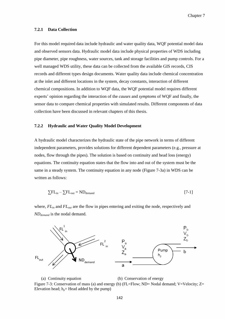
Chapter 7

142

Data Collection 7.2.1

For this model required data include hydraulic and water quality data, WQF potential model data

and observed sensors data. Hydraulic model data include physical properties of WDS including

pipe diameter, pipe roughness, water sources, tank and storage facilities and pump controls. For a

well managed WDS utility, these data can be collected from the available GIS records, CIS

records and different types design documents. Water quality data include chemical concentration

at the inlet and different locations in the system, decay constants, interaction of different

chemical compositions. In addition to WQF data, the WQF potential model requires different

experts’ opinion regarding the interaction of the causes and symptoms of WQF and finally, the

sensor data to compare chemical properties with simulated results. Different components of data

collection have been discussed in relevant chapters of this thesis.

Hydraulic and Water Quality Model Development 7.2.2

A hydraulic model characterizes the hydraulic state of the pipe network in terms of different

independent parameters, provides solutions for different dependent parameters (e.g., pressure at

nodes, flow through the pipes). The solution is based on continuity and head loss (energy)

equations. The continuity equation states that the flow into and out of the system must be the

same in a steady system. The continuity equation in any node (Figure 7-3a) in WDS can be

written as follows:

∑FLin – ∑FLout = NDdemand [7-1]

where, FLin and FLout are the flow in pipes entering and exiting the node, respectively and

NDdemand is the nodal demand.

(a) Continuity equation (b) Conservation of energy

Figure 7-3: Conservation of mass (a) and energy (b) (FL=Flow; ND= Nodal demand; V=Velocity; Z=

Elevation head; hp= Head added by the pump)

FLout

FL1

in

FL2

in

NDdemand

Chapter 7

143

The conservation of energy describes the relationship between the energy loss/ gain and pipe

flow. Let us consider a situation shown in Figure 7-3 (b) where water flows from the node (a) to

the node (b). The pressure, elevation head and the mean velocity at node (a) are Pa, Za and Va,

respectively and the pressure, elevation head and the mean velocity at node (b) are Pb, Zb and Vb,

respectively. Let us also, consider that the total friction and fitting head losses from node (a) to

node (b) are HL, and the pump’s head is hp. The energy conservation equation (Figure 7-3 (b))

can be written as follows:

[7-2]

For WDS with lp loops, pn pipes and nd nodes (pn=lp+nd-1) with pipe diameter dp (p=1, 2 …pn),

pipe length Lp (p= 1, 2 ...pn) and nodal demand, NDn ( n=1, 2, 3 ,.. nd), Equation (7-1) and (7-2)

can be solved to calculate flow and pressures for all pipes and nodes, respectively. In this study,

instead of analytical solutions, EPANET (Rossman 2000) simulation engine has been used to

solve these equations. EPANET uses “hybrid node-loop” approach which is also known as

"Gradient Method"(Rossman 2000). Detail of EPANET simulation algorithm has been described

in the users’ manual of EPANET (i.e., Rossman 2000).

The EPANET simulation engine can also model the water quality behaviour in a WDS over an

extended period of time. The governing equations for solving water quality are based on the

principles of conservation of mass coupled with reaction kinetics (Rossman et al. 1993). The

modelling capacity of the current version of EPANET is limited to just a single chemical specie,

such as free chlorine used in a disinfectant decay study or any chemical having an appropriate

decay rate (including zero decay). However, in reality a WDS needs to deal with multiple

interacting chemical species (Shang and Uber 2008). To address this problem, Shang et al. (2007)

developed a general framework to model the reaction and transport of different interacting

chemicals in a WDS. The developed framework has been implemented as an extension of

EPANET programmer’s toolkit as a library of function which is also referred as EPANET-MSX

(Multi-Species Extension). For this study, modelling of multiple interacting chemical interactions

has been modelled using EPANET-MSX programmers’ toolkit.

In EPANET-MSX, all the reaction dynamics, fast/ equilibrium and conservation of mass, are

expressed using differential-algebraic equations. These differential equations express the

interactions between the bulk species, surface species, and different parameter values. Equations

7-3 to7-5, provide the general form of differential –algebraic equations (Shang et al. 2007):

Chapter 7

144

)p,z,z,x,x(fdt

dxsbsb

b [7-3]

)p,z,z,x,x(gdt

dxsbsb

s [7-4]

)p,z,z,x,x(h0 sbsb [7-5]

where, x and z are the vector of time-varying differential variable and time-varying algebraic

variables, respectively and b and s indicates their association with the bulk water and pipe surface

respectively and p is the time invariant model parameters. To model a set of chemical species,

reactions of these chemical species must the in the above forms. Details of EPANET-MSX is

available with user manual of EPANET-MSX (Shang and Uber 2008).

WQF potential Model development 7.2.3

Details of WQF potential model development and its application have been discussed in Chapter

6. No further discussion has been provided in this chapter.

WQF Detection 7.2.4

In this step, presence of a significant water quality event is identified in the sensor locations.

Using WQF potential model, WQF potentials in the sensor nodes are evaluated over time. From

the variation of WQF potential, the presence of a water quality anomaly can be identified. In

addition, a regular or special laboratory test results could be important source of information to

identify the most probable causes of water quality failure.

Source Tracking Using PEST 7.2.5

After the identification of presence of a contaminant in WDS, the parameter estimation software

package developed by Watermark Numerical Computing, Parameter ESTimation, PEST has

been used to source track the detected contaminant. PEST is the industry standard open source

public domain, model-independent parameter estimation and uncertainty analysis software

package. It has very powerful capacity to manage a large number of parameters and to optimize

different parameters by searching for either the maximum or the minimum value of an objective

function (Baranowski and LeBoeuf 2006). According to Doherty and Hunt (2010), it has the

capacity to accommodate hundreds, or even thousands, of parameters in the calibration /

optimization process without any issue of numerical stability, and it provides a guarantee of

Chapter 7

145

parameter reasonableness. To calibrate or optimize a parameter, it interacts with model input and

output parameters without accessing to the original model algorithm. To optimize the objective

function, PEST uses the Gauss–Marquardt–Levenberg algorithm which evaluates the weighted

sum of squared differences between observed and model computed outputs (Doherty 2005).

Figure 7-4 shows the general workflow of PEST optimization.

Figure 7-4: Work flow of PEST optimization

At the beginning, the original model is simulated using necessary input parameters and hereafter,

PEST compares the observed data with simulated outputs and estimates the weighted sum of

squared differences (WSSD) between observed and simulated outputs. If the estimated WSSD is

not acceptable, PEST changes the input parameter based on the given instructions and simulate

the model again. The acceptability of the WSSD is evaluated by comparing the parameter change

and objective function improvement achieved in the current iteration and previous iterations.

The PEST software package has been used in various model calibrations in various complex

modelling environments. It has been adapted in some popular commercial software to automate

the calibration process of their model (e.g., GMS from AQUAVEU). Bahremand and Smedt

(2008) have used PEST for the sensitivity analysis of the model parameters of a distributed

hydrological model. Numerous applications of PEST have been reported in the literature.

However, most of these applications are related to ground water modelling, hydrological

modelling, or irrigation demand modelling. Baranowski and LeBoeuf (2006) have used different

optimization techniques to evaluate optimal demand to reduce the contaminant concentration in

in a water distribution system. From the comparative analysis of three optimization techniques,

Chapter 7

146

(i) an unconstrained first-order reliability method (FORM) (ii) a constrained FORM; and (iii)

PEST package, Baranowski and LeBoeuf (2006) concluded that the PEST is the best approach

among them with greater capabilities in determining the most optimal solution.

Figure 7-5: Flowchart for PEST implementation to identify the most probable sources of water

quality event

Following the guidelines provided by Khalsa and Ho (2008), PEST has been used to identify the

most probable origin and its ingress rate of the detected contaminant. To identify the origin of a

contaminant source, a list of suspected origins/ sources20 is created. PEST optimizes the water

quality parameter considering all the suspected nodes as a most probable origin of water quality

20

A suspected origin list consists of a set of selected nodes based on any prior information or all the nodes exist

in the water distribution system which could be potential origin of the identified contaminant ingress.

Chapter 7

147

failure. During each optimization, PEST estimates the minimum objective function, the sum of

squared weighted residuals, “Phi” for all the suspected nodes. A suspected node which has the

smallest of the minimum objective functions, “Phi”, is considered as the most probable origin of

contaminant ingress. The estimated concentration for the most probable origin of the contaminant

ingress is also identified during this process. Figure 7-5 shows different steps used for source

tracking.

Severely Affected Area Identification 7.2.6

After the identification of ingress matrix (origin and concentration), hydraulic and water quality

behavior of the WDS have been simulated. This simulation results provide necessary information

to estimate WQF potential in different nodes in the WDS. Due to the nodal physical, chemical

and demand heterogeneity, each node WQF potential has been lumped by multiplying

surrounding water volume at each node in terms of (%-volume). Figure 7-6 shows the zone of

influence of a node used to estimate the volumetric WQF potential.

Figure 7-6: Zone influence

From the volumetric WQF potentials, the relative importance of a node has been evaluated with

respect to the volumetric WQF potentials of the surrounding nodes. During this evaluation OWA

has been applied with the highest weight of given to the node of concern. The procedure has been

applied to the all the nodes or preselected suspected nodes. This will provide a new set

volumetric WQF potentials containing influence of surrounding nodes. Figure 7-7 shows the

different steps involved to identify the most severely affected areas in a WDS. Following above

procedure, a node is identified containing the higher value of volumetric WQF potential which is

nothing but the most severely affected node in the WDS. As a cross check of this approach, the

relative changes of different parameters of a particular node during base condition (normal

Chapter 7

148

quality condition) and a potential failure condition are compared. This comparison can also

identify the most severely affected area in distribution system.

Figure 7-7: Flowchart for detecting the most probable source node of WQ failure

7.3 Model Implementation

To demonstrate the proof of concept, the developed model has been implemented and

demonstrated through an example WDS. Iron based metallic pipes have been intentionally

assumed to represent reaction of arsenic. Water is supplied by gravity from the two elevated

reservoirs (reservoir 1 and reservoir 2) with the total head of 90 m, and 85 m, respectively. The

lengths of the pipes vary from 100 m to 680 m, and the diameters of the pipes vary from 200 mm

to 700 mm. Base demands at different nodes varies from 50 l/s to 100 l/s and demand multipliers

ranges from 0.38 at 5am to 1.46 at 9 am. Detail information on pipe length, diameter, roughness

coefficient, nodal connectivity, and nodal hourly base demand and demand multipliers and two

reservoirs head have been provided in Table 3-6 in Chapter 3.

.

Chapter 7

149

Under normal operating conditions, there is no major quality issue. Initial chlorine concentrations

from both reservoirs ensure the minimum chlorine concentration at all the nodes in the system.

As a hypothetical scenario, an intentional contamination with Arsenic in the WDS is assumed

which react with the disinfectant residual monochloramine (NH2Cl). To avoid modelling

complexity, the initial concentrations of monochloramine at the both reservoirs are also assumed

(2.5µm/L).The hydraulic and water quality conditions are modelled using the EPANET and

EPANET-MSX which estimates hydraulic and water quality properties at nodes and pipes of the

WDS. The additional information which cannot be modelled using EPANET and EPANET–

MSX are considered same used in Chapter 6. The observed data for both normal and arsenic

contamination events have been generated using the EPANET and EPANET–MSX.

Modelling of Fate of Arsenic in WDS 7.3.1

In Chapter 6, a list of 17 parameters has been identified which causes WQF in WDS. It is

impractical to collect data for all the parameters at all locations of a WDS. Therefore, for water

quality modelling, an EPANET-MSX model has been developed. In addition, due to the

modelling complexity, it is difficult to model all the identified interacting water quality

parameters. The proposed methodology has been demonstrated using an example taken from

Shang and Uber (2008) which represents contamination of drinking water by an intentional

injection of arsenic into the WDS.

Figure 7-8: schematic of Arsenic oxidation/ adsorption in the water distribution system (source:

(Shang and Uber 2008)

This example shows the oxidation of the intentional contaminate arsenic from its arsenite (As+3)

to arsenate (As+5) by the influence of monochloramine disinfectant residual in the bulk flow. The

developed EPANET-MSX model simulates the different interacting reactions between arsenic

and monochloramine in bulk flow, boundary layer and pipe surface. Figure 7-8 shows the

schematic of Arsenic oxidation/ adsorption in the water distribution system. The mathematical

Chapter 7

150

form of the reactions has been expressed in terms of five differential rate equations (Gu et al.

1994; Shang and Uber 2008):

)( 2

33

ClNHAskdt

dAsa

[7-6]

)()(

22 ClNHk

dt

ClNHdb

[7-7]

)()(55

2

35

wvfa AsAsAKClNHAskdt

dAs

[7-8]

5

2

55

max1

55

5

)([)(

swsvwvfw AskAsAsSkAAsAsAK

dt

dAs

[7-9]

5

2

55

max1

5

)(

swss AskAsAsSk

dt

dAs

[7-10]

where As+3 is the arsenite concentration in the bulk water, As+5 is the arsenate concentration in

the bulk water, Ass+5

is the arsenate concentration in pipe surface, Asw+5

is the arsenate

concentration adjacent to the pipe wall (bulk), NH2Cl is the monochloramine concentration in the

bulk water, ka is the rate coefficient for the arsenite oxidation, kb is the rate coefficient for

monochloramine decay, Av is the pipe surface area per liter pipe volume, k1 and k2 are the rate

coefficients for arsenate adsorption and desorption respectively, Smax is the maximum pipe

surface concentration of arsenate, and Kf is the mass transfer coefficient dependent of the amount

of turbulence in pipe and diameter of the pipe. The value of Kf is estimated using equation 7-11

shown as follows:

DK f

88.04 Re106.1

[7-11]

where Re is the Reynolds number and D is the diameter of the pipe.

To use EPANET-MSX, reactions are converted in the form of equations 7-3, 7-4 and 7-5.

According to Shang and Uber (2008), in case of reversible sorption processes, a local equilibrium

assumption (LEA) is sometimes assumed between the concentrations in the bulk and the

Chapter 7

151

adsorbed phase (i.e., 0

5

dt

dAss ). Therefore, the equation 7-10 can be expressed as an algebraic

equation as shown in equation 7-12.

5

5

max5

1

Ask

AsSkAs

s

ss

[7-12]

Where ks=k1/k2.

Therefore, the equations 7-6 to 7-9 and equation 7-12 are the required form of reactions (rate

equations and one algebraic equation) which have been modelled using EPANET-MSX. In the

above five equations, the respective terms for equation 7-3, 7-4 and 7-4 are, xb=[As+3,

As+5,Asw+5,NH2Cl], xs=[Ø] , zs=[Ass

+5], p=[ka, kb, Av, k1, k2, Kf, Smax]. A further details of the

modelling multi-species as this example, are available in Shang and Uber (2008).

Figure 7-9: Residual chlorine concentration at nodes 8, 21 and 27

In addition, it is assumed that the chlorine decay is only due the bulk water and wall decay. The

reaction of bulk and wall decay has been modelled using the equation as shown below:

0.55

0.6

0.65

0.7

0.75

0.8

0.85

0 500 1000 1500 2000 2500

Re

sid

ual

Ch

lori

ne

, mg/

l

Time, min

Node 8 Node 21 Node 27

Chapter 7

152

CkkD

kkCk

t

C

fw

fw

b .)(

..4.

[7-13]

where, C is the chlorine concentration, kb is the bulk water decay rate, kw is the pipe water decay

rate, kf is the mass transfer coefficients, D is the pipe diameter. Figure 7-9 shows residual

chlorine at node 8, 21 and 27 for typical two consecutive days.

Water Quality Event Data Preparation 7.3.2

As the proposed methodology has been demonstrated using an example WDS, therefore, the

observed data have been generated by simulating arsenic contamination event using the

EPANET-MSX model. To represent contamination of water due to arsenic ingress, arsenic has

been added in the system constantly at the rate of 10µgm/L randomly from the node no. 7.

Figure 7-10: Total Arsenic concentration at different nodes in the network

0.00

2.00

4.00

6.00

8.00

10.00

12.00

12:00 AM 12:00 AM 12:00 AM 12:00 AM 12:00 AM 12:00 AM 12:00 AM 12:00 AM 12:00 AM 12:00 AM 12:00 AM 12:00 AM

Tota

l A

rsen

ic, µ

m/L

Time (hr:min)

Node 7 Node 18 Node 21 Node 27

Chapter 7

153

The simulation results of any node can be considered as an observed arsenic concentration in that

particular node. For this study, arbitrarily sensors have been assumed in five locations in the

WDS at nodes 4, 18, 21 and 27. The simulated results from these nodes are considered as

observed data and have been used in the source tracking. It is noted that the number of observed

nodes depends on the network size and type of the chemicals. For a successful source tracking,

the contaminant in the system must have impact on the observed data. If the contaminant ingress

can not influence the observed data, the model will not be able to perform its intended objective.

Therefore, optimum number of sensors is required to monitor the observed data. The number of

optimum sensors has not been covered in this thesis. Figure 7-10 shows the time varying total

Arsenic concentration of As+3 at the ingress node (Node 7) and other three nodes (i.e., node no.

18, 21 and 27).

WQF Detection and Source Tracking Using PEST 7.3.3

After the detection of arsenic, PEST has been used to identify the most probable origin of arsenic

in the system. To source track back, PEST package requires three input files which are (a) the

template file (*.tpl) (b) the instruction file (*.ins) and (c) the control file (*.pst).

As a part of optimization, PEST runs the model using various combination of input variables and

minimizes / maximizes its objective function. To change the input variables during optimization,

PEST requires guideline what to change. The template file (*.tpl) is the guideline which tells the

PEST what parameters are required to change. A template file is based on the model input file

which has at least one optimizing parameter. In this case, EPANET-MSX input file ‘*.msx’ is

converted to template file. Detail instruction for the creation of template file has been provided in

Doherty (2005). Instruction file is another prerequisite input file to run PEST package. It provides

instruction to PEST, how to read the simulated data from the output file to compare with the

observed data. In this study, the outputs are taken from EPANET-MSX output file. Again, detail

for creating an instruction file has been provided in Doherty (2005). The third important PEST

input file is a control file. A control file combined everything together including information

from template and instruction files. It assembles the model names and its execution command,

parameter names and their initial values, observed data, template file and corresponding input

file, instruction file, and a number PEST variables which control the implementation of the

Gauss-Marquardt-Levenberg method (Doherty 2005).

After configuring input files, PEST has been run to optimize ingress dose considering node 1

(reservoir 1) as a first suspected node for ingress. It is noted that PEST keeps records for all the

Chapter 7

154

calculation in the “*.rec” file in the PEST simulation directory, and after optimization it left the

input file with the optimized parameters’ values. After the PEST run for the first suspected node,

the PEST “*.rec” file are checked which contains the sum of squared weighted residuals (i.e.,

phi). The optimize parameter for a particular suspected node has the lowest value of “Phi”. For

the first suspected node (i.e., reservoir 1), the estimated minimum value of he sum of squared

weighted residuals (i.e., Phi) =7.417 and the estimated ingress concentration is 9.65µg/L. The

procedure continues for the all the suspected nodes one by one. The most probable source of

ingress node is the one which has an absolute minimum value of “Phi” and corresponding

concentration is the ingress rate. In this example, the estimated absolute minimum value

(minimum value of all minimum values) of sum of squared weighted residuals (i.e., Phi) =

9.0000E-04 and the estimated ingress concentration is 10.0001 µg/L. These values were

estimated considering node 7 as a suspected node which is nothing but the node where the ingress

rate concentration were used to generate observed data. The estimated ingress concentration was

also estimated almost 100% accuracy. The whole procedure has been automated writing a Matlab

program which can finally identify the most probable ingress sources and ingress concentration.

Identification of the Most Severely affected Area in WDS 7.3.4

It is not necessarily always true that the ingress node is the most severely affected area. There are

many contaminants which have growth inside the WDS, especially, microbiological

contaminants. For this type of contaminants the most severely affected node could be the node

other than the origin of the contaminant. In that case, after the identification of the most probable

location and dose of contaminant ingress, EPANET-MSX model have been used to simulate the

contaminant at the different location of WDS. The most severely affected area need to be

identified used WQF potential model as described earlier. However, in this case, as the arsenic

has no growth inside the distribution system, therefore, the ingress node 7 was also identified as

the most severely affected node in the system. However, during an attempt to simulate bacterial

intrusion in the distribution system, it was found that node 27 is the most severely affected node

due to microbial contamination in the distribution system.

7.4 Model Summary

This chapter discussed the WQF detection and diagnosis methodology. The model has a capacity

to identify the presence of any contaminant intrusion into a WDS. It has also capacity to identify

the most probable origin of the contaminant intrusion and a most possible ingress rate in the

Chapter 7

155

system. It also has the capacity to identify the most severely affected area in the WDS. The

developed model has been implemented on an example WDS to demonstrate its applicability for

arsenic intrusion from a single ingress node. From the analysis, it is seen that the developed

model can fulfill its objectives by detecting presence of contaminant intrusion and its ingress

matrix. The developed model can be used for any real WDS by modifying appropriate factors /

parameters. Although the proposed methodology can detect and diagnosis a water quality event

in WDS, however, interaction multiple chemical ingress has not been investigated. The detection

methodology is based on the change in output parameters. Therefore, if the ingress rate is very

small and or ingress contaminant reacts very slowly there might be some difficulty in detection.

Chapter 7

156

CHAPTER 8 INTEGRATED DICISION SUPPORT

SYSTEM

8.1 Introduction

An integrated prognostic and diagnostic analysis framework consisting of various novel models and

existing best management practice tools has been proposed in Chapter 2. The development of

different models and their standalone applications through case studies have been discussed in

Chapter 3 to Chapter 7. In this chapter, a methodology has been developed to integrate the outputs of

the developed models and existing available information. Although different models have been

developed under the framework of fuzzy set theory, the integration of the developed models has

been carried out under the framework of Dempster–Shafer (D-S) theory of evidence (Shafer 1976).

One of the most important reasons for switching from Fuzzy set theory to the D-S theory is the

number of parameters involved in different models. Using fuzzy set theory, it was difficult to make

the integrated framework sensitive to different parameters due to the huge volume of data. However,

D-S theory provides better results in this case.

8.2 Integration Framework

Figure 8-1 shows the conceptual integration of the proposed framework. This framework is a holistic

view of the WDS system management tools. According to the different modes of failures, the

integration process has been categorized into hydraulic and water quality components. However,

based on the modes of investigation, the integration process has been categorized as prognostic

investigation and diagnostic investigation. Considering modes of failures and types of investigations,

the integration process has four parts consisting of hydraulic prognostic investigation (H, P),

hydraulic diagnostic investigation (H, D), water quality prognostic investigation (Q, P), and water

quality diagnostic investigation (Q, D). For the hydraulic prognostic investigation, integrated

hydraulic state of the WDS has been evaluated based on the outputs of leakage potential model,

calculated hydraulic utility (disutility) model and historical pipe burst data. The sources of this

information have been mentioned at the bottom of relevant boxes in Figure 8-1.

Chapter 8

157

Figure 8-1: Conceptual integration of proposed framework

Chapter 8

158

Details of leakage potential model have been described in Chapter 4, and as part of the reliability

assessment methodology, the evaluation of hydraulic utility has been described in Chapter 3. It is

noted that in the integration process, instead of hydraulic utility, hydraulic disutility which is the

complement of hydraulic utility has been used. The historical pipe burst information has been

used as an external source of information from the utility regular data repository. The hydraulic

diagnostic investigation which identifies the most probable location of hydraulic failure is based

on the hydraulic state of WDS (prognostic investigation), customer complaints and leakage

propensity evaluated in Chapter 5. Although evaluated leakage propensity can identify the most

probable location of hydraulic failure independently, the integration of customer complaints and

prognosis investigation results will enhance the confidence on the decision.

Similar to the hydraulic state, integrated water quality state of WDS has been evaluated based on

the outputs of WQF potential model, water quality utility (disutility) model and historical WQF

data. Development and evaluation of WQF potential and WQ utility have been described in

Chapter 6 and Chapter 3, respectively. Similar to the hydraulic disutility, the water quality

disutility has been used in the water quality state estimation. The historical water quality failure

data have been used as an external source of information from the utility regular data repository.

The water quality diagnostic investigation identifies the most severely affected locations in a

WDS based on the water quality state of the WDS (prognostic investigation), customer

complaints and available laboratory water quality test results. The information coming from the

different models has been used directly in the integration process. However, historical pipe burst

data, historical WQF data, hydraulic and water quality customer complaints and water quality

laboratory test results have been harmonized. Due to the variation of the importance of data in

space and data type, the two adaptation factors called, Equivalent on Spot Complaints (ESC) and

Equivalent Illness Complaints (EIC) have been introduced. While ESC has been used to

harmonize the spatial issues, EIC has been used to harmonize different types of water quality

complaints and laboratory test results. The concepts of ESC, EIC and D-S theory of evidences

and their implementation in the integration process have been described in the following sections.

Finally, based on the outputs of the model results and harmonized data, an integrated decision

support system has been developed.

8.3 Equivalent on Spot Complaint (ESC)

The different types of complaints received by water companies are spatially distributed. As Bicik

et al. (2011) mentioned that the customer complaints are strong indicators of water distribution

Chapter 8

159

failure, however, all of them are not trustworthy with a same confidence level. A complaint

received from the spot of the failure shall have a higher level of confidence than a complaint

received from other than the failure location.

Figure 8-2: Variation of an ESC with complaint distance and constant, a.

To address spatial heterogeneities, different complaints such as pipe burst complaints and water

quality complaints have been converted to an equivalent on spot complaint (ESC). An ESC has

been defined as a complaint which has a confidence level equivalent to a complaint reported from

the spot of the failure. Equation 8-1 has been used to estimate an ESC of a complaint:

axeESC [8-1]

where, a is a constant based on the expert opinion, x is the Euclidian distance from the

complaining customer to the candidate node/ pipe in km. Figure 8-2 shows the variation of ESC

under variable x and a. Although x is constant for a particular complaint, a decision maker has no

control over it, however, a decision maker can model his attitude to the confidence level by

controlling the parameter, a.

0

0.1

0.2

0.3

0.4

0.5

0.6

0.7

0.8

0.9

1

0 0.5 1 1.5 2 2.5 3 3.5 4 4.5 5

Eq

uiv

alen

t on S

pot

Com

pla

int (E

SC

)

x in km

a=0.5

a=1

a=2

a=3

Chapter 8

160

8.4 Equivalent Illness Complaints (EIC)

In Chapter 6, a list of nine symptoms and 17 causes of water quality failure has been identified. A

water company may receive customer complaints for any of these water quality failure issues,

even further. However, the severities of these complaints are not same. A complaint for bad taste

does not have the same severity for a complaint for reported water born disease. To address the

variation of different types of water quality complaints, a common scale termed as Equivalent

Illness Complaint (EIC) has been introduced. An EIC has been defined as a water quality

complaint which has a severity level equivalent to a complaint that causes illness for the

customers. Equation 8-2 has been used as measured EIC of a water quality complaint.

)1,0(W,where,WCEIC i

N

1i

ii

[8-2]

where i is the different types of complaints, Ci is the number of different types of complaints, and

Wi is the weight of the each complaint with respect to a complaint of illness to the customer.

Although a decision maker has no control on the number of different types of complaints,

however, a decision maker can model his attitude by controlling Wi based on their expert

judgments.

8.5 Dempster–Shafer Theory

Dempster-Shafer (D-S) theory is a mathematical evidence theory and considered as a

generalization of the Bayesian approach (Sadiq et al. 2006a). The groundbreaking work was

introduced by Dempster (1967) and extended by Shafer (1976). In the Bayesian approach, the

summation of a “hypothesis”, p (A), and a “not hypothesis”, p (not A), is one, (i.e., p (A) + p (not

A) =1). Based on this relationship, a belief in a hypothesis A can be used to derive the belief in its

complement without any evidence of its complement. In this case, ‘‘not A’’ is the missing

evidence (lack of knowledge) but this complement, ‘‘not A’’ is evaluated with an equal

confidence of “p (A)”. Therefore, some researchers argued that ‘‘no evidence’’ is different from

having degree of confidence in a certain hypothesis and this argument is the basic motivation

behind D–S theory of evidence. In D-S theory, evidence is attributed in the form of belief to the

subsets in a universe of discourse (). For example, if some evidence “a” is attribute of p (A), the

ignorance ‘‘1 -a’’ will not be assigned to p (not A), rather it will be assigned to both {p (A), p

(not A)}. D-S theory has been used in various engineering applications including water related

Chapter 8

161

applications. Sentz and Ferson (2002) provided a background discussion on D-S theory and a

review of different applications of this theory in various fields. Application of this theory in the

field of water engineering is relatively new but not rare. Sadiq et al. (2006) used D-S theory to

estimate the risk of contaminant intrusion in WDS. Li (2007) used D-S theory for hierarchical

risk assessment of water supply system. Bicik et al. (2011) used D-S theory to fuse information

collected from three different models to identify the most probable location of burst in a WDS.

Sadiq and Rodriguez (2005) discussed basic concepts of D-S theory and applied to interpret

drinking water quality in WDS.

Three important concepts - basic probability assignment, belief function, and plausibility are the

souls of D-S theory and operates under on a ‘‘frame of discernment’’, . The “frame of

discernment’’ is a set of mutually exclusive alternatives, the space of possible events / options. A

belief assigned to each individual exclusive alternative is termed as a basic probability

assignment; also known as mass function and expressed as: BPA (A), bpa (A) or m (A). A basic

probability assignment function (2 →[0, 1]) satisfies the following conditions:

i. all the beliefs are mapped in the interval of [0 1] , i.e., m (A)→[0 1]

ii. the null set is ‘‘0’’ , i.e., m(φ)=0

iii. the sum of basic probability assignments in a given set A is ‘‘1’, i.e., ∑ ( )

Another important component of the D-S theory is a belief function (bel) which is the sum of all

basic probability assignments of all subsets (B) of the set (A), and mathematically, can be

expressed as ( ) ∑ ( ) Based this relationship, it is also possible to prove that

( ) and ( ) . The third important function of D-S theory is the plausibility

function (pl) which is nothing but the upper limit of belief and the sum of all basic probability

assignments of all subsets (B) that intersects with the set of interest (A), and mathematically, can

be expressed as ( ) ∑ ( ) ( ) For the basic discussion to detail interpretation on the

D-S theory, readers are suggested to consult with different D-S theory based literature (e.g., Bicik

et al. 2011; Li 2007; Sadiq et al. 2006; Sadiq and Rodriguez 2005).

Estimation of BPAs 8.5.1

In this study, D-S theory has been implemented to evaluate hydraulic & the water quality state of

WDS (prognosis) and diagnostic investigation of different kind hydraulic & water quality

failures. In all cases, the frame of discernment consists of two propositions (binary frame of

Chapter 8

162

discernment) of different kinds of failures, and described by a universal set, Θ= {L, NL} where L

represents likelihood and NL represents not likelihood of different kind of incidences. The power

set of incidences consists of the following subsets: (ɸ, {L}, {NL}, {L, NL}). In case of hydraulic

failure, {L} represents the likelihood of hydraulic failure; {NL} represents the not likelihood of

hydraulic failure and {L, NL} represents complete ignorance about hydraulic failure. In a similar

way, the water quality failure frame of discernment has been implemented where {L} represents

the likelihood of water quality failure; {NL} represents not likelihood of water quality failure and

{L, NL} represents complete ignorance about water quality failure.

The proposed integration framework (Figure 8-1) has four different phases. In each phase, three

different sources of evidences have been used. Table 8-1 shows different sources of evidences

used in different phases of integration and their sources of evidences.

Table 8-1: Different phase of Integration

Phases Phase names Evidences Location of Evidence

Phase 1 Hydraulic prognosis

(H, P)

Leakage potential model

Hydraulic utility model

Historical pipe burst data

Pipe

Node

Pipe

Phase 2 Hydraulic diagnosis

(H, D)

Customer complaints

Hydraulic state

Leakage propensity

Pipe/Node

Pipe/Node

Pipe/Node

Phase 3 Quality prognosis

(Q, P)

WQF potential model

Water quality utility model

Historical WQF data

Node

Node

Pipe

Phase 4 Quality diagnosis (Q,

D)

Customer complaints

Water quality state

Laboratory results

Pipe/Node

Pipe/Node

Pipe/Node

In Table 8-1, it is mentioned that some evidences are available along the pipe lengths, some are at

nodes, and some can be available both along pipes and at the nodes. For example, the leakage

potential and the historical pipe bursts evidences are available along the pipes whereas the

hydraulic utilities are evaluated at different nodes. However, the prognostic and diagnostic

investigation can be carried out using either nodal or pipe evidences. Therefore, either the nodal

evidences are required to convert to the pipe evidences or the pipe evidences required convert to

Chapter 8

163

the nodal evidences. In this case, the nodal evidences are converted to pipe evidences by

averaging nodal evidences of two connecting nodes and the pipe evidences are converted using

zone influences estimated by the half of the connecting pipe length to a node (Figure 7-6).

In both cases, evidences are harmonized based on the appropriate adjustment factors (ESC &

EIC). In case of evidence available along a pipe, Euclidian shortest distance from the complaint

location to the pipe location, and in case of evidence available at a node, Euclidian shortest

distance from the complaint location to the node have been used in ESC and EIC calculation.

From the homogenized evidences, the BPAs have been evaluated using two step procedure

adapted from Safranek et al. (1990). The technique is quite popular and adapted by several

investigators in the literature (Bicik et al. 2011; Gerig et al. 2000). However, a fuzzy based

approach us also reported in the literature (Sadiq et al. 2006).

At the first step of BPAs estimation, the historical pipe bursts, customer complaints, historical

WQFs, laboratory results and leakage propensities have been converted to normalized confidence

factors using a suitable normalization function. However, leakage potential, WQF potential,

hydraulic and water quality utility are already in a scale of (0, 1), therefore, further

normalizations are not necessary for them. Numerous (e.g., Sigmoid, Gaussian, Logit, and even a

Linear) normalization functions can be used to estimate equivalence confidence factors.

However, for this study, a sigmoid function has been adapted. Equation 8-3 shows the sigmoid

function used for normalization (Beynon 2005; Gerig et al. 2000):

)v(ki,jiii,jie1

1)v(cf

[8-3]

where ki describes the steepness of the function and θi determines the offset of v axis. The

solutions of this function are controlled by two controlling variables, ki and θi. According to

Safranek et al. (1990), above function satisfy following criteria:

(i) cfi(vj,i) is a monotonic increasing (or decreasing) function.

(ii) cfi(vj,i) =1; if the measurement v implies certainty in the hypothesis

(iii) cfi(vj,i) =0; if the measurement v implies certainty in not the hypothesis

(iv) cfi(vj,i) =0.5; if the measurement v favors neither the hypothesis nor not the hypothesis.

The normalized evidences in different phases have been mapped to BPAs for {L}, {NL} and {L,

NL} using the following equations (Equation 8-4, 8-5, and 8-6):

Chapter 8

164

2i,ji1

i,ji2

21

11i,ji

21

1

i,ji

i,j

A1)v(cf,B

1A)v(cfA1,AA1

BA)v(cf

AA1

B

1A)v(cf,0

})L({m

[8-4]

3i,ji2

4i,ji3

43

234i,ji

3

4i,ji3

i,j

A1)v(cf,B

A)v(cfA1,AA1

]BB][A)v(cf[B

A)v(cf,B

})NL({m

[8-5]

})NL({m})L({m1})NL,L({m i,ji,ji,j

[8-6]

The equations 8-4, 8-5, and 8-6 are controlled by one variable and seven controlling parameters

(A1, A2, A3, A4, B1, B2, and B3; 1). A decision maker can define these controlling parameters

based on their expert judgment. Figure 8-3 shows definition of the controlling variables and the

general steps for the transformation of input data into BPAs.

Figure 8-3: Transformation of data into BPAs (adapted from Beynon 2005)

After conversion of evidences into BPAs, combination rules have been applied to evaluate the

joint evidences of different kinds of failures.

Chapter 8

165

Rules of Combination 8.5.2

In D-S theory, the evidences from multiple sources are integrated using combination rules. The

Dempster’s rule of combination rule was originally used in the D-S theory. However, various

other combination rules have been developed by different investigators over the time. In addition

to Dempster’s rule, other combination rules include the Mixing or Averaging Rule, Yager’s

Modified Dempster’s Rule, Inagaki’s Unified Combination Rule, Zhang’s Center Combination

Rule, Dubois and Prade’s Disjunctive Consensus Rule and so forth (Sentz and Ferson 2002). In

this study, the Dempster’s rule of combination has been used which combines two BPAs, m1 and

m2 and estimates the joint BPA, m1-2 emphasizing on the agreement of the sources of evidences

and ignoring the conflicting evidence (Sentz and Ferson 2002). Equation 8-7 expresses the

mathematical formula of Dempster’s combination rule (Klir and Folger 1988):

CB

21

21

ACB

21

21

)C(m)B(mKwhere

0)(mand

;AwhenK1

)C(m)B(m

)A(m

[8-7]

The term K represents the degree of conflict between two different sources B and C and 1-K is

the normalization factors.

It is convenient to employ Dempster’s combination rule between two evidences. However,

evidences often come from more than two sources which are not possible to implement in a

single rule at a time. For example, three sources of evidences exist in all phases of this

integration. In this situation, Dempster’s combination rule has been employed by cascading

different evidences. Figure 8-4 shows the general cascade application of Dempster’s combination

rule between the multiple sources of evidences. Initially, Dempster’s rule is applied between two

evidences and joint BPAs ({L}, {NL}, {L, NL}) are evaluated which is considered as a single

evidence. Hereafter, Dempster’s rule is applied between combined single evidence and third

evidence. The process continues until the last evidence is combined.

Chapter 8

166

Figure 8-4: Cascade application of Dempster's rule

8.6 Implementation of Decision Support System

In different chapters of this thesis, the development of different models and their implementations

have been described in details, however, fragmentally. This section describes a comprehensive

proof-of-evidence of the developed integrated DSS under normal operating condition and under

failure condition. The integration process has been demonstrated using the WDS described in

Chapter 3.

Data Preparation 8.6.1

The implementation of the DSS depends on the model dependent secondary data and additional

primary data as additional evidences. The model dependent secondary data include leakage

potential, WQF potential, hydraulic utility, water quality utility and indices of leakage propensity

in different nodes. The additional primary data include historical pipe bursts & water quality

failures, recent customer complaints, and water quality laboratory test reports. The historical

water quality failures and recent water quality complaint parameters include the number of

reported illness, color and turbidity, drop of free residual chlorine and odor and so forth (Table

6-8). Recent customer complaints include pipe bursts and water quality complaints received from

different customers. For the all recent complaints, distances from the source of complaints have

been considered and recorded. In case of laboratory test report, the sample locations (i.e.,

distances) with respect to the nearest node / pipe also have been considered as recorded

evidences. Since the leakage potential (Chapter 4) model and WQF potential (Chapter 6) model

Chapter 8

167

have been demonstrated using the different WDS than the network used in this chapter, a typical

average values of leakage potential and the WQF potential have been used in all cases.

Table 8-2: Primary data used in the integration phase

Pip

e/N

od

e

nu

mb

er

No

. of

pip

e b

urs

t

Lea

kag

e p

ote

nti

al

His

tori

cal

qual

ity

fail

ure

(n

odal

)

No

dal

WQ

F

po

ten

tial

s

1 0 0.34 0 0.27

2 0 0.41 0 0.38

3 1 0.37 0 0.31

4 0 0.33 0 0.30

5 0 0.45 1 0.44

6 0 0.35 0 0.28

7 0 0.42 0 0.37

8 1 0.33 2 0.26

9 0 0.48 0 0.42

10 0 0.42 0 0.33

11 0 0.34 1 0.32

12 1 0.36 2 0.35

13 0 0.49 5 0.49

14 0 0.49 2 0.39

15 0 0.41 1 0.39

16 0 0.38 0 0.34

17 0 0.32 0 0.26

18 0 0.38 0 0.36

19 1 0.31 1 0.24

20 0 0.31 0 0.30

21 1 0.36 0 0.32

22 0 0.31 0 0.21

23 0 0.38 0 0.32

24 0 0.45 2 0.37

25 3 0.49 0 0.44

26 0 0.48

27 0 0.47

28 0 0.48

29 2 0.48

30 0 0.49

31 0 0.31

32 1 0.40

33 0 0.37

34 3 0.48

35 0 0.43

36 0 0.36

37 4 0.40

38 0 0.50

39 3 0.50

40 1 0.40

Chapter 8

168

The other parameters such as hydraulic utility & water quality utility and ILPs have been used as

same as described earlier in Chapter 3 and Chapter 5. Table 8-2 shows the assumed number of

pipe bursts and leakage potentials for different pipes and historical water quality failure events

and WQF potentials in different nodes. The network failure condition has been simulated by

disconnecting the failed pipe from the remaining network which has been modelled in EPANET

by making pipe’s initial status to ‘close’. In this case, pipe 29 was modelled as a failed pipe.

From Chapter 3, it was found that customers can get full hydraulic utility from the WDS under

the normal condition. However, in case of a failure (pipe 29), there is an issue of hydraulic

disutility in some nodes. Due to the pipe 29 failure, the most critical duration of the day is 6-8 am

and during this period, the WDS has highest demand multiplier of 1.49. The estimated hydraulic

disutility at nodes 18, 22, 23, 24 and 25 during the period of 6-8 am are 0.976, 0.192, 1, 1 and 1,

respectively. However, other nodes have full utilities during the day. It is noted that in spite of

WDS failure, no violation of desired water quality utility was observed during the day. Under the

normal operating condition, it is expected that the WDS will continue to operate without any

hydraulic and quality customer complaints or any positive laboratory test results. However, in

failure condition, it is expected that utility company will receive different kinds of customer

complaints based on type of failures. In case of water quality events, the water company itself

may find some quality issues in their regular laboratory test programs. To mimic the failure

condition, customer complaints are assumed in different locations of WDS over the time.

Table 8-3: Non-zero primary data under failure condition

Time

/Node

No.

Reported cumulative customer complaints Non-compliance lab. report

Pipe

bursts

Illness Colors FRC Turbidity

20 21 12 13 19 24 12 13 15 17 19 25 13 26 27 11 13 17 21

0-2 0 1 2 2 1 3 1 2 1 2 1 2 1 1 1 1 1 1 1

2-4 0 1 3 3 1 3 1 2 1 2 1 3 1 1 1 1 1 1 1

4-6 2 1 3 4 1 3 1 2 1 2 1 4 1 1 1 1 1 1 1

6-8 3 1 3 5 1 3 1 2 1 2 1 5 1 1 1 1 1 1 1

8-10 4 1 3 6 1 3 1 2 1 2 1 5 1 1 1 1 1 1 1

10-12 4 1 3 6 1 3 1 2 1 2 1 5 1 1 1 1 1 1 1

12-14 4 1 3 6 1 3 1 3 1 2 1 5 1 1 1 1 1 1 1

14-16 4 1 3 6 1 3 1 3 1 2 1 5 1 1 1 1 1 1 1

16-18 4 1 3 6 1 3 1 3 1 2 1 5 1 1 1 1 1 1 1

18-20 4 1 3 6 1 3 1 3 1 2 1 5 1 1 1 1 1 1 1

20-22 4 1 3 6 1 3 1 3 1 2 1 5 1 1 1 1 1 1 1

22-24 4 1 3 6 1 3 1 3 1 2 1 5 1 1 1 1 1 1 1

Chapter 8

169

Table 8-3 shows non-zero primary data under hydraulic and water quality failure conditions as

additional evidences. The values of these parameters at other nodes which are not provided in

Table 8-3 are zeros. It is also noted that the distances from the complaint sources to the candidate

nodes varies. For simplicity, all the distances have been considered as a single value of 0.3 km.

Table 8-4 shows a list of assumed controlling parameters used to convert different complaints to

the relevant ESC and EIC. All of these parameters have been assumed based on the expert

judgment. The values of these parameters can vary one expert to another expert, however, impact

of the variations should not be significant to dilute the model results.

Table 8-4: Assumed constants to convert ESC & EIC

Parameters Coefficients

a w

Pipe burst 2 -

Illness 2 1

Color 2 0.5

Drop of FRC 2 0.6

Turbidity 2 0.7

Estimation of BPAs 8.6.2

After gathering relevant data, the BPAs are evaluated following the procedure described in

section 8.5.1. Primary data are normalized using a sigmoid function as shown in Equation 8-3.

The leakage potential, WQF potential, hydraulic and water quality utility are in a range of [0 1]

and no further normalization is necessary.

Table 8-5: Controlling parameters for normalization and BPAs estimation

Controlling Parameters Normalization BPAs

k θ A1 A2 A3 A4 B1 B2 B3

Leakage potential - - 0.1 0.1 0.1 0.1 0.8 0.1 0.5

Hydraulic utility - - 0.1 0.1 0.1 0.1 0.8 0.1 0.5

Historical pipe burst 0.5 1 0.1 0.1 0.1 0.1 0.8 0.1 0.5

WQF potential - - 0.2 0.1 0.1 0.1 0.8 0.1 0.5

Water quality utility - - 0.2 0.1 0.1 0.1 0.8 0.1 0.5

Historical WQF 0.1 2 0.2 0.1 0.1 0.1 0.8 0.1 0.5

Hydraulic customer

complaints 0.3 1.5

0.1 0.1 0.2 0.1 0.9 0.1 0.5

Leakage propensity 0.3 1.5 0.1 0.1 0.2 0.1 0.9 0.1 0.5

Water quality customer

complaints 0.9 2

0.0 0.1 0.1 0.1 1.0 0.1 0.4

Laboratory results 0.9 2 0.0 0.1 0.1 0.1 0.7 0.1 0.7

Chapter 8

170

The normalization of different evidences is controlled by two parameters ( ki & θi) whereas the

BPAs are controlled by seven parameters (A1, A2, A3, A4, B1, B2, and B3). For the evaluation of

the state of different components of a WDS, the values of the controlling parameters required

careful selection. Table 8-5 shows the different controlling parameters used for the normalization

and the BPAs estimation in this demonstration. Using the normalized values of different

evidences, the BPAs are evaluated using equations 8-4, 8-5, and 8-6. After the estimation of

individual BPAs, the Dempster rule combination has been applied.

Results and Discussion 8.6.3

8.6.3.1 Hydraulic Prognostic Investigation (H, P)

The hydraulic prognosis analysis is based on the performance measure of WDS in past, present

and future conditions which are reflected in historical pipe bursts, hydraulic disutility, and

leakage potential of different nodes, respectively. Based on these evidences, the state of WDS for

a likely failure, not likely failure and ignorance (likely or not likely) of failure under normal

operating condition as well as under failure condition have been estimated. Table 8-6 shows the

hydraulic prognosis results of top four likely pipes (in order) under normal condition. The pipes

with the most likely, the 2nd, the 3rd, and the 4th most likely chances of failure are no. 34, 39,

37, and 25, respectively. The values of {L} and {NL} are complementary. If a node has highest

{L} value, it has lowest {NL} value among all the nodes. It is observed that the {L} values have

proportional relation to the available pressure profile and inverse relation with the available water

demand. The time period of 6-8 am has the highest demand multiplying factor (i.e., maximum

demand) and, therefore, lowest available pressure. During this period the {L} is lowest and {NL}

highest which indicates lower chances of failure. It is understandable that at low pressure, the

chance of a pipe failure is minimal. However, in this model, this relationship is valid until the

nodal hydraulic utilities are to a certain limit. In any case, hydraulic utility falls down from the

desired level, the prognosis results shows the increase of chances for failures, in spite of pressure

drop. This has been reflected from a similar solution under a failure condition.

Table 8-7 shows the hydraulic prognosis results of top four likely pipes (in order) under failure

condition. This table also shows that under the failure condition, the prognosis results changed in

a certain extent in all time steps. However, the changes in different pipes during the period of 6-8

am are drastic compared to the other time steps because of the extreme pressure drop which has

reduced the hydraulic utility in a considerable extent.

Chapter 8

171

Table 8-6: Hydraulic prognosis results of top four likely pipes (in order) under normal condition

Time

(hour)

First Second Third Fourth

Pipe No. {L} {NL} {L, NL} Pipe No. {L} {NL} {L, NL} Pipe No. {L} {NL} {L, NL} Pipe No. {L} {NL} {L, NL}

0-2 34 0.50 0.43 0.06 39 0.46 0.48 0.07 37 0.44 0.49 0.07 25 0.39 0.53 0.08

2-4 34 0.50 0.44 0.06 39 0.45 0.48 0.07 37 0.44 0.49 0.07 25 0.39 0.53 0.08

4-6 34 0.45 0.48 0.07 39 0.39 0.53 0.08 37 0.39 0.54 0.08 25 0.35 0.57 0.08

6-8 34 0.34 0.57 0.08 37 0.29 0.63 0.09 25 0.28 0.63 0.09 39 0.28 0.63 0.09

8-10 34 0.39 0.54 0.08 37 0.33 0.59 0.08 39 0.33 0.59 0.08 25 0.31 0.60 0.09

10-12 34 0.40 0.53 0.08 37 0.34 0.58 0.08 39 0.34 0.58 0.08 25 0.32 0.60 0.09

12-14 34 0.43 0.50 0.07 39 0.38 0.55 0.08 37 0.37 0.55 0.08 25 0.34 0.57 0.08

14-16 34 0.45 0.48 0.07 39 0.40 0.53 0.08 37 0.39 0.53 0.08 25 0.36 0.56 0.08

16-18 34 0.41 0.52 0.07 37 0.35 0.57 0.08 39 0.35 0.57 0.08 25 0.33 0.59 0.08

18-20 34 0.40 0.52 0.07 37 0.34 0.57 0.08 39 0.34 0.57 0.08 25 0.32 0.59 0.08

20-22 34 0.42 0.51 0.07 39 0.36 0.56 0.08 37 0.36 0.56 0.08 25 0.33 0.58 0.08

22-24 34 0.45 0.49 0.07 39 0.39 0.53 0.08 37 0.39 0.54 0.08 25 0.35 0.57 0.08

Table 8-7: Hydraulic prognosis results of top four likely pipes in order under failure condition

Time (hour) First Second Third Fourth

Pipe No. {L} {NL} {L, NL} Pipe No. {L} {NL} {L, NL} Pipe No. {L} {NL} {L, NL} Pipe No. {L} {NL} {L, NL}

0-2 34 0.53 0.42 0.06 25 0.43 0.50 0.07 29 0.43 0.50 0.07 39 0.42 0.51 0.07

2-4 34 0.52 0.42 0.06 25 0.43 0.50 0.07 29 0.43 0.50 0.07 39 0.42 0.51 0.07

4-6 34 0.47 0.47 0.07 25 0.39 0.53 0.08 29 0.39 0.54 0.08 39 0.36 0.56 0.08

6-8 34 0.86 0.12 0.02 39 0.79 0.18 0.03 40 0.71 0.25 0.04 25 0.56 0.39 0.06

8-10 34 0.41 0.52 0.07 25 0.35 0.57 0.08 29 0.34 0.58 0.08 39 0.29 0.62 0.09

10-12 34 0.42 0.51 0.07 25 0.36 0.56 0.08 29 0.35 0.57 0.08 39 0.30 0.61 0.09

12-14 34 0.45 0.48 0.07 25 0.38 0.54 0.08 29 0.38 0.55 0.08 39 0.34 0.58 0.08

14-16 34 0.47 0.46 0.07 25 0.40 0.53 0.08 29 0.39 0.53 0.08 39 0.36 0.56 0.08

16-18 34 0.43 0.50 0.07 25 0.36 0.56 0.08 29 0.36 0.56 0.08 39 0.31 0.60 0.09

18-20 34 0.43 0.50 0.07 25 0.36 0.56 0.08 29 0.35 0.56 0.08 39 0.31 0.60 0.09

20-22 34 0.44 0.49 0.07 25 0.37 0.55 0.08 29 0.36 0.56 0.08 39 0.32 0.59 0.08

22-24 34 0.47 0.47 0.07 25 0.39 0.53 0.08 29 0.39 0.54 0.08 39 0.35 0.56 0.08

Chapter 8

172

Table 8-8: Hydraulic diagnosis results of top four likely nodes (in order) under normal condition

Time (hour) First

Second

Third

Fourth

Node No. {L} {NL} {L, NL} Node No. {L} {NL} {L, NL} Node No. {L} {NL} {L, NL} Node No. {L} {NL} {L, NL}

0-2 25 0.55 0.44 0.01

20 0.49 0.49 0.02

27 0.41 0.58 0.02

24 0.38 0.60 0.02

2-4 25 0.54 0.44 0.01

20 0.49 0.49 0.02

27 0.40 0.58 0.02

24 0.38 0.60 0.02

4-6 25 0.49 0.49 0.02

20 0.44 0.54 0.02

27 0.35 0.63 0.02

24 0.34 0.64 0.02

6-8 25 0.39 0.59 0.02

20 0.36 0.62 0.02

7 0.29 0.69 0.02

15 0.28 0.70 0.02

8-10 25 0.43 0.55 0.02

20 0.40 0.58 0.02

15 0.30 0.68 0.02

7 0.29 0.68 0.02

10-12 25 0.44 0.54 0.02

20 0.41 0.58 0.02

15 0.30 0.68 0.02

24 0.30 0.68 0.02

12-14 25 0.47 0.51 0.02

20 0.43 0.55 0.02

27 0.33 0.65 0.02

24 0.33 0.65 0.02

14-16 25 0.49 0.49 0.02

20 0.45 0.53 0.02

27 0.35 0.63 0.02

24 0.34 0.64 0.02

16-18 25 0.45 0.53 0.02

20 0.41 0.57 0.02

24 0.31 0.67 0.02

27 0.31 0.67 0.02

18-20 25 0.45 0.54 0.02

20 0.41 0.57 0.02

24 0.31 0.67 0.02

15 0.30 0.67 0.02

20-22 25 0.46 0.52 0.02

20 0.42 0.56 0.02

27 0.32 0.66 0.02

24 0.31 0.66 0.02

22-24 25 0.49 0.50 0.02 20 0.44 0.54 0.02 27 0.34 0.63 0.02 24 0.34 0.64 0.02

Table 8-9: Hydraulic prognosis results of top four likely nodes (in order) under failure condition

Time (hour) First

Second

Third

Fourth


0-2 20 0.69 0.30 0.01

25 0.54 0.45 0.01

27 0.39 0.59 0.02

17 0.39 0.59 0.02

2-4 20 0.70 0.29 0.01

25 0.55 0.44 0.01

27 0.40 0.58 0.02

17 0.38 0.60 0.02

4-6 20 0.66 0.33 0.01

25 0.49 0.49 0.02

17 0.36 0.62 0.02

27 0.35 0.63 0.02

6-8 20 0.93 0.06 0.00

25 0.85 0.15 0.00

27 0.75 0.24 0.01

26 0.71 0.28 0.01

8-10 20 0.66 0.33 0.01

25 0.41 0.57 0.02

17 0.33 0.65 0.02

15 0.31 0.67 0.02

10-12 20 0.67 0.32 0.01

25 0.42 0.57 0.02

17 0.33 0.65 0.02

15 0.31 0.67 0.02

12-14 20 0.71 0.28 0.01

25 0.46 0.52 0.02

17 0.35 0.63 0.02

15 0.33 0.65 0.02

14-16 20 0.72 0.27 0.01

25 0.48 0.50 0.02

17 0.36 0.62 0.02

15 0.34 0.64 0.02

16-18 20 0.68 0.31 0.01

25 0.43 0.55 0.02

17 0.34 0.64 0.02

15 0.32 0.66 0.02

18-20 20 0.67 0.32 0.01

25 0.42 0.56 0.02

17 0.33 0.64 0.02

15 0.31 0.67 0.02

20-22 20 0.69 0.30 0.01

25 0.44 0.54 0.02

17 0.34 0.64 0.02

15 0.32 0.66 0.02

22-24 20 0.71 0.28 0.01 25 0.47 0.51 0.02 17 0.36 0.62 0.02 22 0.34 0.64 0.02

Chapter 8

173

It is noted that the failure condition has been created by assigning a leakage demand at node 20.

However, from the topology of the network and the top four most likely failure pipes, it is

perceived that the identified leakage node is no. 25 which is not true. Hence, from the hydraulic

prognosis results, it is not possible to identify the leaky node. However, an informed guess can be

made about the presence of leakage in the system. If the network continues to run without any

failure events, a daily prognosis results should not change significantly. To identify the failure

location, a diagnostic investigation is necessary which have been discussed in later on in this

chapter.

8.6.3.2 Hydraulic Diagnostic Investigation (H, D)

Similar to the prognosis analysis, the diagnostic hydraulic analysis has been carried out. The

hydraulic diagnostic analysis is based on the hydraulic prognosis analysis results / hydraulic state

of WDS, customers’ complaints and estimated leakage propensities at different nodes. Based on

these evidences, likely failure, not likely failure and ignorance (likely or not likely) of failure of

particular condition have been estimated. Following the methodology described previously, Table

8-8 shows the hydraulic diagnosis results of the top four likely nodes (in order) under normal

condition. From

Table 8-7 and Table 8-8, it is evident that, in the normal condition, both diagnostic and prognostic

investigation identifies the same node as the most probable location of failure. As no significant

changes in the BPAs ({L}, {NL}, {L, NL}) from normal operating BPAs are not observed, it

does provide any indication of failure in the system. However, under the failure condition, from

Table 8-9, it is realized that the diagnostic investigation results have changed in a considerable

extent indicating a probable failure in the system. Most importantly, it is perceived (

Table 8-9) that the diagnostic investigation results have identified different node (Node 20) as the

most probable leaky node in the system which was the leaky node synthetically created by

assigning an extra leakage demand.

8.6.3.3 Water Quality Prognostic Investigation (H, P)

Similar to the hydraulic prognosis and diagnosis analysis, water quality prognosis and diagnosis

analysis have been carried out. Following the methodology described earlier, Table 8-10 shows

the water quality prognosis results under normal condition. From Table 8-10, it is seen that the

chances of water quality failure during the first few hours are extremely high. This is because, the

Chapter 8

174

water quality utility during the first couple of hours are very low due to low residual chlorine

concentration in different nodes. This lower residual chlorine concentration was due to travel

time of source residual chlorine (a simulation issue). However, in reality, this does not happen as

the WDS supplies water after enough water flushing and if the network is simulated for an

existing operating condition, initial residual chlorine concentration will show up from the

beginning of the simulation. Therefore, it is required to avoid couple of hour simulation results.

Actual results will show up after these periods which have been reflected in Table 8-10. From

Table 8-10, it is found that the pipe 15 has highest chances of water quality failure. It is noted

that, as described in Chapter 3, due to the hydraulic failure at a node, no impact on water quality

failures were observed because the hydraulic changes did not impact the water quality failure in

the distribution system in this case. However, to check the sensitivity of the water quality

prognosis model, a minor change was incorporated (5% increase) of water quality failure

potential under normal condition. From that case, changes are also observed in the chances of

water quality failure. However, the changes were not enough to change the ranking of nodes for

the chances of failure. Table 8-11 shows the water quality prognosis results of the top four likely

nodes (in order) under minor changes in WQF potentials.

8.6.3.4 Water Quality Diagnostic Investigation (Q, D)

Similar to the water quality prognosis analysis, the water quality diagnostic analysis has been

carried out. The diagnostic analysis is based on the quality prognosis analysis results / water

quality state of WDS, customers’ complaints and routine / special laboratory test results. Based

on these evidences, likely failure, not likely failure and ignorance (likely or not likely) of failure

of particular condition have been estimated. Following the methodology described previously,

Table 8-12 shows the water quality diagnosis results of the top four likely nodes (in order) under

normal condition. From Table 8-10, Table 8-11and Table 8-12, it is patent that in the normal

condition, both diagnostic and prognostic investigations nodes identify the same node as a most

probable failure location. As no significant changes in the BPAs ({L}, {NL}, {L, NL}) from

normal condition are observed, it does not provide indication of failure in the system. However,

under the failure condition, from Table 8-13, it is evident that the diagnostic investigation results

have changed in considerable extents indicating a probable failure in the system. Most

importantly, it is seen (Table 8-13) that the diagnostic investigation results identify the different

node (Node 13) as the most probable location of water quality failure in the system which is

consistent with the received customer complaints and laboratory test results.

Chapter 8

175

Table 8-10: Water quality prognosis results of top four likely nodes (in order) under normal condition

Time (hour) First

Second

Third

Fourth


0-2 27 0.81 0.16 0.03

26 0.79 0.18 0.03

25 0.76 0.20 0.04

20 0.67 0.28 0.05

2-4 27 0.32 0.57 0.11

15 0.27 0.62 0.11

11 0.26 0.63 0.11

16 0.25 0.64 0.11

4-6 15 0.27 0.62 0.11

11 0.26 0.63 0.11

27 0.26 0.63 0.11

16 0.25 0.64 0.11

6-8 15 0.27 0.62 0.11

11 0.26 0.63 0.11

27 0.26 0.63 0.11

16 0.25 0.64 0.11

8-10 15 0.27 0.62 0.11

11 0.26 0.63 0.11

27 0.26 0.63 0.11

16 0.25 0.64 0.11

10-12 15 0.27 0.62 0.11

11 0.26 0.63 0.11

27 0.26 0.63 0.11

16 0.25 0.64 0.11

12-14 15 0.27 0.62 0.11

11 0.26 0.63 0.11

27 0.26 0.63 0.11

16 0.25 0.64 0.11

14-16 15 0.27 0.62 0.11

11 0.26 0.63 0.11

27 0.26 0.63 0.11

16 0.25 0.64 0.11

16-18 15 0.27 0.62 0.11

11 0.26 0.63 0.11

27 0.26 0.63 0.11

16 0.25 0.64 0.11

18-20 15 0.27 0.62 0.11

11 0.26 0.63 0.11

27 0.26 0.63 0.11

16 0.25 0.64 0.11

20-22 15 0.27 0.62 0.11

11 0.26 0.63 0.11

27 0.26 0.63 0.11

16 0.25 0.64 0.11

22-24 15 0.27 0.62 0.11 11 0.26 0.63 0.11 27 0.26 0.63 0.11 16 0.25 0.64 0.11

Table 8-11: Water quality prognosis results of top four likely nodes (in order) under minor changes in WQF potentials

Time (hour) First

Second

Third

Fourth


0-2 27 0.82 0.15 0.03

26 0.80 0.17 0.03

25 0.77 0.19 0.03

20 0.68 0.27 0.05

2-4 27 0.34 0.55 0.11

15 0.29 0.61 0.11

11 0.27 0.62 0.11

16 0.27 0.62 0.11

4-6 15 0.29 0.61 0.11

11 0.27 0.62 0.11

27 0.27 0.62 0.11

16 0.27 0.62 0.11

6-8 15 0.29 0.61 0.11

11 0.27 0.62 0.11

27 0.27 0.62 0.11

16 0.27 0.62 0.11

8-10 15 0.29 0.61 0.11

11 0.27 0.62 0.11

27 0.27 0.62 0.11

16 0.27 0.62 0.11

10-12 15 0.29 0.61 0.11

11 0.27 0.62 0.11

27 0.27 0.62 0.11

16 0.27 0.62 0.11

12-14 15 0.29 0.61 0.11

11 0.27 0.62 0.11

27 0.27 0.62 0.11

16 0.27 0.62 0.11

14-16 15 0.29 0.61 0.11

11 0.27 0.62 0.11

27 0.27 0.62 0.11

16 0.27 0.62 0.11

16-18 15 0.29 0.61 0.11

11 0.27 0.62 0.11

27 0.27 0.62 0.11

16 0.27 0.62 0.11

18-20 15 0.29 0.61 0.11

11 0.27 0.62 0.11

27 0.27 0.62 0.11

16 0.27 0.62 0.11

20-22 15 0.29 0.61 0.11

11 0.27 0.62 0.11

27 0.27 0.62 0.11

16 0.27 0.62 0.11

22-24 15 0.29 0.61 0.11 11 0.27 0.62 0.11 27 0.27 0.62 0.11 16 0.27 0.62 0.11

Chapter 8

176

Table 8-12: Water quality diagnosis results of top four likely nodes (in order) under normal condition

Time (hour) First

Second

Third

Fourth


0-2 27 0.86 0.14 0.00

26 0.85 0.15 0.00

25 0.83 0.17 0.00

20 0.75 0.24 0.01

2-4 27 0.46 0.52 0.01

15 0.41 0.57 0.01

11 0.40 0.58 0.01

16 0.40 0.59 0.01

4-6 15 0.41 0.57 0.01

11 0.40 0.58 0.01

27 0.40 0.59 0.01

16 0.40 0.59 0.01

6-8 15 0.41 0.57 0.01

11 0.40 0.58 0.01

27 0.40 0.59 0.01

16 0.40 0.59 0.01

8-10 15 0.41 0.57 0.01

11 0.40 0.58 0.01

27 0.40 0.59 0.01

16 0.40 0.59 0.01

10-12 15 0.41 0.57 0.01

11 0.40 0.58 0.01

27 0.40 0.59 0.01

16 0.40 0.59 0.01

12-14 15 0.41 0.57 0.01

11 0.40 0.58 0.01

27 0.40 0.59 0.01

16 0.40 0.59 0.01

14-16 15 0.41 0.57 0.01

11 0.40 0.58 0.01

27 0.40 0.59 0.01

16 0.40 0.59 0.01

16-18 15 0.41 0.57 0.01

11 0.40 0.58 0.01

27 0.40 0.59 0.01

16 0.40 0.59 0.01

18-20 15 0.41 0.57 0.01

11 0.40 0.58 0.01

27 0.40 0.59 0.01

16 0.40 0.59 0.01

20-22 15 0.41 0.57 0.01

11 0.40 0.58 0.01

27 0.40 0.59 0.01

16 0.40 0.59 0.01

22-24 15 0.41 0.57 0.01 11 0.40 0.58 0.01 27 0.40 0.59 0.01 16 0.40 0.59 0.01

Table 8-13: Water quality diagnosis results of top four likely nodes (in order) under failure condition

Time (hour) First

Second

Third

Fourth


0-2 27 0.87 0.13 0.00

26 0.86 0.14 0.00

25 0.83 0.16 0.00

24 0.80 0.19 0.00

2-4 27 0.49 0.50 0.01

13 0.46 0.53 0.01

12 0.45 0.54 0.01

15 0.43 0.55 0.01

4-6 13 0.48 0.51 0.01

12 0.45 0.54 0.01

15 0.43 0.55 0.01

27 0.42 0.56 0.01

6-8 13 0.50 0.49 0.01

12 0.45 0.54 0.01

15 0.43 0.55 0.01

27 0.42 0.56 0.01

8-10 13 0.52 0.47 0.01

12 0.45 0.54 0.01

15 0.43 0.55 0.01

27 0.42 0.56 0.01

10-12 13 0.52 0.47 0.01

12 0.45 0.54 0.01

15 0.43 0.55 0.01

27 0.42 0.56 0.01

12-14 13 0.52 0.47 0.01

12 0.45 0.54 0.01

15 0.43 0.55 0.01

27 0.42 0.56 0.01

14-16 13 0.52 0.47 0.01

12 0.45 0.54 0.01

15 0.43 0.55 0.01

27 0.42 0.56 0.01

16-18 13 0.52 0.47 0.01

12 0.45 0.54 0.01

15 0.43 0.55 0.01

27 0.42 0.56 0.01

18-20 13 0.52 0.47 0.01

12 0.45 0.54 0.01

15 0.43 0.55 0.01

27 0.42 0.56 0.01

20-22 13 0.52 0.47 0.01

12 0.45 0.54 0.01

15 0.43 0.55 0.01

27 0.42 0.56 0.01

22-24 13 0.52 0.47 0.01 12 0.45 0.54 0.01 15 0.43 0.55 0.01 27 0.42 0.56 0.01

Chapter 8

177

8.7 Summary

In this chapter, developed models have been integrated under the framework of Dempster- Shafer

theory of evidences which makes the whole project as a complete DSS. The developed DSS has

capacities for diagnostic and prognostic investigation of water distribution failure by

communicating different models and their inputs and outputs. It can estimate the likeliness, not

likeliness and complete ignorance (likely, not likely) of different kind of failures in the

distribution system. The developed model has been applied to a WDS. To implement the DSS,

secondary data estimated using different developed models described in different chapters of this

thesis and addition primary data have been generated. From the demonstration, it is evident that

the DSS has capabilities for integrated prognosis and diagnosis investigation of a WDS failure.

Although the developed DSS has been implemented to relatively small WDS for the proof of

concept, however, the developed DSS can be used for any WDS by modifying appropriate

factors/parameters.

Chapter 9

178

CHAPTER 9 CONCLUSIONS AND RECOMMENDATION

9.1 Conclusions

The main objective of this research was to reduce the likelihood of failure in WDS and in case of

a failure, minimize the consequences of the failure. To achieve this objective an integrated

framework has been developed. The developed framework has ‘unique’ capacity to bring

different sources of information under a common framework for prognostic analysis and

diagnostic investigation. The prognostic capability of the framework increases the confidence in

predictive analysis which helps to reduce likelihood of failure. The diagnostic capabilities of the

framework reduce false positive and negative prediction, and identify the failure location with

minimal time after the occurrence which minimizes the consequences of failure. The outcomes of

this research comprehensively addressed the uncertainties associated with WDS which improves

the efficiency and effectiveness of diagnosis and prognosis analyses. The framework brings the

modelling information, customer complaints and laboratory test information under a single

platform.

The foundation stones of the developed framework are five ‘novel’ models which interact and

complement each other under the framework. Among the five models three of them are prognosis

model and two of them are diagnosis model. The first model is the reliability assessment model

which addressed some of the missing components of the traditional reliability assessment. This

model evaluates reliability and provides a measure of uncertainty in the estimated reliability

which ultimately helps to design an absolutely reliable WSS. For the first time, this model

provides an option to the designer to select the level of uncertainties in the network reliability. In

addition, the developed methodology is generic and can be easily implemented in similar types of

infrastructures including oil & gas network, telecommunication network and so forth. An article

based on this model has been submitted for publication in ASCE Journal of Water Resource

Planning and Management.

The developed second model introduces the concept of “leakage potential” and develops a

methodology to evaluate leakage potential in a WDS or a component of WDS. The model shows

a unique way to evaluate the impacts of different influencing factors in leakage. The model

Chapter 9

179

brings the pressure dependent background leakage under a risk based methodology which has not

been seen in the literature. From model implementation results, it reveals that among different

influencing factors, some of the factors have more influence than others. It is identified that in a

certain range, the operating system pressure and age of the network are the most important

factors contributing to LP. For example, for the existing network condition in Bangkok, the

network LP is not very sensitive to low operating pressure (17.9 psi). However, when pressure

exceeds 30 m (42.9 psi), the network LP is more sensitive to the operating system pressure. The

impact of age to LP is very gradual for the current operating system pressure of 12.56 m (17.9

psi). However, if the operating pressure, for example, increases to 45 m (64.3 psi), the LP will

increase more noticeably for same age and other parameters combination. For higher operating

pressure, LP is more sensitive in the age range of 30 - 60 years. An article based on this model

has been published in the IWA Journal of Water Supply: Research and Technology – AQUA [].

The developed third model identifies the presence of leakage, in case of a leakage; it can detect

the position of a leakage in the nearest node / pipe of the WDS. To develop this model, fuzzy set

has been used beyond its traditional application. The developed model is so efficient that it can

identify a small hydraulic change in the WDS. In addition, this methodology introduces a new

concept of ‘indices of leakage propensity’ which provide a measure of severity of the leakage in a

WDS. An article based on this model has been published in Urban Water Journal [8 (6), 351–

365].

The fourth model evaluates the WQF potential in WDS. The developed model identifies 17

“causes” against nine “symptoms” of water quality failure. This model has the capabilities to

make “causes” and “symptoms” relationship which helps to evaluate WQF potential and relative

importance of different water quality parameters. From the sensitivity analysis, it is found that the

pipe age and material are the most sensitive parameters after the coliform. The pH is the least

sensitive “cause” of WQF. An article based on this model has been submitted for publication in

the Water Resource Management.

The fifth model is extended from the WQF potential. The developed model identifies presence of

any water quality event based on the sensory information using the WQF potential model. After

detecting the presence of WQF event, the model source tracks the most probable origin of the

detected contaminant. Finally, the model identifies the most vulnerable area resulting from WQF

and identifies the most probable reason.

Chapter 9

180

All the efforts made to develop different diagnostic and prognostic models are merged into the

integrated decision support system which combines different models, their inputs and output from

the developed models. It has the capacities for diagnostic and prognostic investigation of water

distribution failure and can estimates the likeliness, not likeliness and complete ignorance (likely,

not likely) of failures in the distribution system.

9.2 Recommendations

In spite of significant efforts to reduce WDS failure, a large number of failure events, both SHF

and WQF, occur every year. The main reason of these failures is the difficulties of understanding

of spatially distributed WDS and its different uncertain parameters. In this research, a significant

effort has been made for a better understanding and for a better modelling of WDS and its

uncertain parameters. Following my significant efforts, the main recommendation for conducting

research in this area goes further for better understanding and modelling of WDS uncertain

parameters.

Proposed Framework 9.2.1

Concentrating on the main objective of this research, the framework developed in this

research does not consider the consequences of failures. To avoid lumping of the failure

likelihood with consequences, the consequences of failures have been intentionally

avoided. However, the consequence is a very important part to prioritize rehabilitation

strategies. Therefore, the developed framework can be extended by incorporating

consequences component of risk which will increase the capacity of the proposed

framework.

All the developed models have been developed under the framework of fuzzy set theory

and integration of different models have been conducted under the Dempster- Shafer

theory of evidences. However, the performances of the models and their integration under

other frameworks might be an interesting idea.

Due to data limitation, the different models of the developed framework have been

implemented in different WDS. Comprehensive implementation of the proposed

framework to a single real WDS will be interesting.

Different components of the proposed framework have been developed fragmentally and

each model is a standalone application. However, an integrated DSS has been developed

using the previously developed model results. However, it will be very interesting to

Chapter 9

181

develop software with all the capabilities described in this thesis. A conceptual

integration of developed models with remote telemetry units (RTU), communication

system, and database management system and field support system has been provided in

9.2.3 in this chapter later. Materialization of such software application will be pleasing to

me.

Developed Models 9.2.2

All the models developed can be easily integrated with GIS or USEPA developed EPANET

water distribution system modelling. Such integration will help users to use the developed

models. To integrate with commercially available renounced software, further modification is

necessary.

Specific recommendations include:

In the reliability assessment model, uncertainties have been considered for three

parameters. Further inclusion of uncertain parameters will increase the confidence of the

results.

In the reliability assessment model, the main focus was related to the reliability of WSS.

However, integration of reliability, robustness and resilience (K. Zhang et al. 2012) of a

WSS will be a very interesting idea.

Developed models deal with a large number of parameters and require intense

computational efforts. Specially, reliability assessment and leakage location detection

models are highly computation intensive. A reduction of computational efforts will make

easier application of these models. Using multicore computer or network computer grid

can solve this problem without much difficulty.

In the leakage potential model, effects of different influential factors have been model

based on a single decision maker approach. Inclusion of other decision maker’s attitude

might increase the confidence of the models. In addition, data on the effects of different

influential factors are very limited. Collection of additional information on different

influential factors will increase confidence in the model.

In the WQF potential model, three decision makers participated in the evaluation process.

However, the inclusion of additional decision makers’ inputs might increase the model

reliability.

Chapter 9

182

Like almost all of the risk-based modelling approaches, it is difficult to validate different

models developed. Further study on the validation of different models will increase the

confidence of different models.

To demonstrate the integration of the proposed framework, pipe burst, water quality

failure, laboratory test results are synthetically generated. Implementation of the

developed model with real world problem will enhance the acceptance of the developed

models

Decision Support System 9.2.3

The findings of this research are worth to create independent software as a decision support

system. The development of independent standalone commercial software was out of scope of

this research. However, a conceptual architecture for a commercial package development has

been provided. Figure 9-1 shows the conceptual architecture for a potential DSS based on this

thesis.

Figure 9-1: Conceptual architecture of proposed DSS

Chapter 9

183

The proposed architecture has six components, namely, field installation system, communication,

database management system, central processing unit, and decision and field support. A field

installation system consists of remote terminal units (RTU) and different kinds of sensors such as

pressure sensors, water quality sensors. A RTU is a microprocessor-controlled electronic device

that will interface with the different kinds of sensors and central monitoring system through a

communication system21. The collected data are managed and used in a database management

system which will be used for computation, visualization and interpretation of results. Different

kinds of data management systems include GIS system, CIS system, water quality and data

models and a computational repository for temporary data storage during the computation

process through the central processing units. All of the collected, transported and stored data will

feed the central processing unit (CPU) of the DSS. The CPU is the main component of this thesis

which has been described in different chapters of this thesis. The integration of different

component of the CPU has been described in Chapter 8.

Finally, based on the DSS results, the user will take informed decisions and take necessary action

in the field. All the stage described in the commercial architecture can be easily materialized with

necessary but existing expertise. In addition to the different components described in the

architecture, different existing knowledge to estimate volume of water lost, financial loss due to

water quality failure can be investigated.

21

A communication system can be manual data transportation, or different kind of telecommunication system

such as GSM (Global System for Mobile Communications) network, GPRS (General packet radio service)

wireless system, PSTN (public switched telephone network) telephone line or any other communication system.

Bibliography

184

BIBLIOGRAPHY

ADB & IWP. (2010). Every drop counts: Learning from good practices in eight Asian cities.

Mandaluyong City, Philippines: ADB and IWP-LKYSP. Asian Development Bank and

Institute of Water Policy, Lee Kuan Yew School of Public Policy.

APHA. (1999). American Public Health Association, Method 5910: Standard method for the

examination of water and wastewater, 20th Edition, Washington, DC, USA.

AWWA. (2005). Computer Modeling of Water Distribution Systems - Manual of Water Supply

Practices, 2nd Edition, Denver, USA. American Water Works Association (AWWA).

Aksela, K., Aksela, M., and Vahala, R. (2009). “Leakage detection in a real distribution network using a SOM.” Urban Water Journal, Taylor & Francis, 6(4), 279–289.

Alegre, H. (1999). “Performance Indicators for Water Supply Systems – Current Trends and On-

going Projects, pp. 148-178, Drought Management Planning in Water Supply Systems”, Ed. by Carbera, E., and Garcia-Serra, J., Kluwer Publishers, Netherlands.”

Allen, M. J., Edberg, S. C., and Reasoner, D. J. (2004). “Heterotrophic plate count bacteria–what

is their significance in drinking water?” International journal of food microbiology, Elsevier, 92(3), 265–274.

Arunraj, N., and Maiti, J. (2009). “A methodology for overall consequence modeling in chemical industry.” Journal of hazardous materials, Elsevier, 169(1-3), 556–574.

Babel, M. S., Islam, M. S., DAS, G., and others. (2009). “Leakage management in a low-pressure

water distribution network of Bangkok.” Water science and technology: water supply, IWA

Publishing, 9(2), 141–147.

Bahremand, A., and Smedt, F. D. (2008). “Distributed hydrological modeling and sensitivity

analysis in Torysa Watershed, Slovakia.” Water Resources Management, 22(3), 393-408.

Baranowski, T., and LeBoeuf, E. (2006). “Consequence management optimization for

contaminant detection and isolation.” Water resources planning and management, 132(4), 274-282.

Berry, D., Xi, C., and Raskin, L. (2006). “Microbial ecology of drinking water distribution systems.” Current opinion in biotechnology, Elsevier, 17(3), 297–302.

Besner, M. C., Gauthier, V., Barbeau, B., Millette, R., Chapleau, R., and Prevost, M. (2001).

“Understanding distribution system water quality.” Journal American Water Works Association, AWWA, 93(7), 101–114.

Beynon, M. J. (2005). “A novel technique of object ranking and classification under ignorance:

An application to the corporate failure risk problem.” European Journal of Operational

Research, 167(2), 493-517.

Bibliography

185

Bicik, J. (2010). “A Risk-Based Decision Support System for Failure Management in Water Distribution Networks.” PhD thesis, University of Exeter.

Bicik, J., Kapelan, Z., Makropoulos, Christos, and Savić, D. a. (2011). “Pipe burst diagnostics using evidence theory.” Journal of Hydroinformatics, 13(4), 596.

Boxall, J B, and A J Saul. 2005. “Modeling discoloration in potable water distribution systems.” ASCE Journal of Environmental Engineering 131(5):716-725.

Brans, J. P., Vincke, P., and Mareschal, B. (1986). “How to select and how to rank projects: The

PROMETHEE method.” European Journal of Operational Research, North-Holland, 24(2),

228–238.

Charron, D., Thomas, M., Waltner-Toews, D., Aramini, J., Edge, T., Kent, R., Maarouf, A., and

Wilson, J. (2004). “Vulnerability of waterborne diseases to climate change in Canada: a review.” Journal of toxicology and environmental health. Part A, 67(20-22), 1667-77.

Cheung, P., Zyl, J. Van, and Reis, L. (2005). “Extension of epanet for pressure driven demand

modeling in water distribution system.” Proceedings of CCWI2005 - Water Management for

the 21st Century. Exeter, UK, pp. 215-226, Center for Water Systems, University of Exeter, vol. 1, Exeter,, UK, 311.

Chowdhury, S., Champagne, P., and Husain, T. (2007). “Fuzzy risk-based decision-making

approach for selection of drinking water disinfectants.” Journal of water supply: research

and technology-AQUA, IWA, 56(2), 75–93.

Corso, P. S., Kramer, M. H., Blair, K. A., Addiss, D. G., P., J. addix, and Davis, C., A. (2003).

“Cost of Illness in the 1993 Waterborne Cryptosporidium Outbreak, Milwaukee, Wisconsin.” Emerging Infectious Diseases, 9(4), 426-431.

Covas, D., Ramos, H., and Almeida, A. B. De. (2005). “Standing wave difference method for

leak detection in pipeline systems.” ASCE Journal of Hydraulic Engineering, 131 (12), 1106-1016.

Deb, A. (1995). Distribution system performance evaluation. American Water Works

Association Research Foundation, Denver, Colorado.

Dempster, A. (1967). “Upper and lower probabilities induced by a multivalued mapping.” The Annals of Statistics, (28), 325-339.

Doherty, J. (2005). PEST—model independent parameter estimation, user’s manual, 5th Ed., Watermark Numerical Computing, Brisbane, Australia.

Doherty, J., and Hunt, R. (2010). Approaches to highly parameterized inversion: a guide to using

PEST for groundwater-model calibration, Technical Report, US Geological Survey

Scientific Investigations Report 2010–5169, 2010.

Dunning, D., Ross, Q., and Merkhofer, M. (2000). “Multiattribute utility analysis; best

technology available; adverse environmental impact; Clean Water Act; Section 316(b). Environ Sci Policy 3:7–14.”

Bibliography

186

Eaton, A. D., and Franson, M. A. H. (2005). Standard methods for the examination of water &

wastewater, Washington, DC, USA. American Public Health Association (APHA), the

American Water Works Association (AWWA), and the Water Environment Federation

(WEF).

Egerton, A. J. (1996). “Achieving reliable and cost effective water treatment.” Water Science and

Technology, Elsevier, 33(2), 143–149.

Engelhardt, M., Skipworth, P., Savic, D., Saul, A., and Walters, G. (2000). “Rehabilitation

strategies for water distribution networks: a literature review with a UK perspective.” Urban Water, Elsevier, 2(2), 153–170.

Fang, W., Hu, J., and Ong, S. (2010). “Effects of phosphorus on biofilm disinfections in model drinking water distribution systems.” Journal of water and health, 8(3), 446-454.

Fang, W., Hu, J. Y., and Ong, S. L. (2009). “Influence of phosphorus on biofilm formation in

model drinking water distribution systems.” Journal of applied microbiology, 106(4), 1328-35.

Fares, H., and Zayed, T. (2009). “Risk Assessment for Water Mains Using Fuzzy Approach.”

Building a Sustainable Future - Proceedings of the 2009 Construction Research Congress,

ASCE, 1125-1134.

Farley, B., Mounce, S., and Boxall, J. (2010). “Field testing of an optimal sensor placement

methodology for event detection in an urban water distribution network.” Urban Water Journal, Taylor & Francis, 7(6), 345–356.

Farley, M. (2001). Leakage management and control: A best practice training manual. WHO, Geneva, Switzerland.

Farley, M., and Trow, S. (2003). Losses in water distribution networks: a practitioner’s guide to assessment, monitoring and control. (First, ed.), IWA Publishing.

Fisher, I., Kastl, G., Sathasivan, A., and Jegatheesan, V. (2011). “Suitability of chlorine bulk

decay models for planning and management of water distribution systems.” Critical Reviews

in Environmental Science and Technology, 41(20), 1843-1882.

Francisque, Alex., Rodriguez, M.J., Sadiq, R., Miranda, L. F., and Proux, F. (2009). “Prioritizing

monitoring locations in a water distribution network: a fuzzy risk approach.” Journal of water supply: research and technology-AQUA, IWA, 58(7), 488–509.

Francisque, Alex., Rodriguez, Manuel J., Miranda-Moreno, L. F. L. F., Sadiq, R., and Proulx, F.

(2009). “Modeling of heterotrophic bacteria counts in a water distribution system.” Water research, Elsevier, 43(4), 1075-87.

Frauendorfer, R., and Liemberger, R. (2010). The issues and challenges of reducing non-revenue water, Asian Development Bank, Philippines.

Fujiwara, O., and Ganesharajah, T. (1993). “Reliability assessment of water supply systems with

storage and distribution networks.” Water Resources Research, American Geophysical Union, 29(8), 2917–2924.

Bibliography

187

Furness, R. (2003). “Assessing Leakage in Water Supply Networks Using Flowmeters.” Water Engineering & Management (March 2003), 150(3), 26-29.

Fuzzy Logic Toolbox 2- User’s Guide. (2011). “Fuzzy Logic Toolbox-Design and simulate fuzzy

logic systems, Mathworks, Natick, MA. Website: http://www.mathworks.com/products/fuzzylogic/, Last Visited 12 October, 2011.”

Gad, A., and Farooq, M. (2001). “Application of fuzzy logic in engineering problems.” Industrial

Electronics Society, 2001. IECON’ 01, The 27th Annual Conference of the IEEE, IEEE, 2044–2049.

Gerig, G., Welti, D., Guttmann, C., and Colchester, A. (2000). “Exploring the discrimination

power of the time domain for segmentation and characterization of active lesions in serial MR data.” Medical Image Analysis, 4(1), 31- 42.

Gregory, R. (1990). “Galvanic corrosion of lead solder in copper pipework.” Water and Environment Journal, John Wiley & Sons, 4(2), 112–118.

Greyvenstein, B., and Zyl, J. Van. (2007). “An experimental investigation into the pressure-

leakage relationship of some failed water pipes.” Journal of Water Supply: Research and

Technology, AQUA, IWA Publishing, Commerce Way, Colchester, CO 2 8 HP, UK,, 56(2),

117–124.

Gu, B., Schmitt, J., Chen, Z., and Liang, L. (1994). “Adsorption and desorption of natural organic

matter on iron oxide: mechanisms and models.” Journal of Environmental Science & Technology, 28(1), 38-46.

Gupta, R., and Bhave, P. R. (1994). “Reliability analysis of water distribution systems.” Journal of Environmental Engineering, 120(2), 447-460.

Gupta, R., and Bhave, P. R. (2007). “Fuzzy parameters in pipe network analysis.” Civil Engineering and Environmental Systems, Taylor & Francis, 24(1), 33–54.

Haestad Methods, I., Walski, T. M., Chase, D. V., Savic, D. A., Grayman, W., Beckwith, S., and

Koelle, E. (2003). Advanced water distribution modeling and management. Haestad

Methods Inc, Waterbury, CT 06708-1499.

Health Canada. (2002). “Canadian Communicable Diseases Report.” Technical report :28, 94-95.

Health Canada. (2003). “Copper. In: Guidelines for Canadian drinking water quality. Supporting

documentation. Ottawa, Ontario.” Water Quality and Health Bureau, Healthy Environments and Consumer Safety Branch, Health Canada, Ottawa, Ontario.

Howard, G., Godfrey, S., Tibatemwa, S., and Niwagaba, C. (2005). “Water safety plans for piped

urban supplies in developing countries: a case study from Kampala, Uganda.” Urban Water

Journal, Taylor & Francis, 2(3), 161–170.

Howarth, D. (1998). “Arriving at the economic level of leakage: Environmental aspects.” Water

and Environment Journal, Wiley Online Library, 12(3), 197–201.

Bibliography

188

Hwang, C. L., and Yoon, K. (1981). Multiple attribute decision making: methods and applications: a state-of-the-art survey. Springer-Verlag New York.

IPCS. (1998). “Copper. Geneva, World Health Organization, International Programme on Chemical Safety (Environmental Health Criteria 200).”

Islam, M. S. (2005). “Leakage Analysis and Management in the Water Distribution Network in a

Selected Area of Bangkok. Master of Engineering Thesis, Asian Institute of Technology,

Thailand.”

Islam, M. S., Sadiq, R., Rodriguez, M.J., Francisque, A., Najjaran, H., and Hoorfar, M. (2011a).

“Water Distribution System Failure: A Forensic Analysis.” Submitted for publication to the

Journal of Tunnelling and Underground Space Technology (TUST) incorporating Trenchless Technology Research.

Islam, M. S., Sadiq, R., Rodriguez, M.J., Francisque, A., Najjaran, H., and Hoorfar, M. (2011b).

“Leakage Detection and Location in Water Distribution System using a Fuzzy-Based Methodology.” Urban Water Journal, 8(6), 351-365.

Islam, M. S., Sadiq, R., Rodriguez, M.J., Francisque, A., Najjaran, H., and Hoorfar, M. (2011c).

“Evaluating Water Quality Failure Potential in Water Distribution Systems: A Fuzzy-

TOPSIS-OWA Based Methodology.” Submitted for publication to the Journal of Water Resource Management.

Islam, M. S., Sadiq, R., Rodriguez, M.J., Francisque, A., Najjaran, H., and Hoorfar, M. (2011d).

“Leakage Forensic Analysis for Water Distribution Systems: A Fuzzy-Based Methodolog.”

the 20th Canadian Hydrotechnical CSCE Conference, Ottawa, Ontario, Canada, June 14-17, 2011.

Islam, M. S., Sadiq, R., Rodriguez, M.J., Francisque, A., Najjaran, H., Naser, B., and Hoorfar, M.

(2012a). “Evaluating Leakage Potential in Water Distribution Systems: A Fuzzy-Based

Methodology.” Accepted for publication to the Journal of Water Supply: Research and

Technology – AQUA, 61(4):240–252.

Islam, M. S., Sadiq, R., Rodriguez, M.J., Najjaran, H., and Hoorfar, M. (2012b). “Reliability

assessment for water supply systems: a novel methodology.” Submitted for publication to the Journal of water resources planning and management.

Jacquet-Lagreze, E., and Siskos, J. (1982). “Assessing a set of additive utility functions for

multicriteria decision-making, the UTA method.” European journal of operational research, Elsevier, 10(2), 151–164.

Jowitt, P., and Xu, C. (1993). “Predicting pipe failure effects in water distribution networks.” Journal of water resources planning and management, 119, 18-31.

Karanis, P., Kourenti, C., and Smith, H. (2007). “Waterborne transmission of protozoan parasites:

a worldwide review of outbreaks and lessons learnt.” Journal of water and health, 5(1), 1-

38.

Keeney, R. L., and Raiffa, H. (1976). Decisions with multiple objectives: Preferences and value

trade offs. Cambridge Univ Pr.

Bibliography

189

Khan, F. I., and Sadiq, R. (2005). “Risk-based prioritization of air pollution monitoring using

fuzzy synthetic evaluation technique.” Environmental monitoring and assessment, Springer, 105(1), 261–283.

Khatri, K., and Vairavamoorthy, K. (2007). Challenges for urban water supply and sanitation in the developing countries, UNESCO-IHE Institute for education, Delft, The Netherlands.

Kingdom, B., Liemberger, R., and Marin, P. (2006). The Challenge of Reducing Non-Revenue

Water ( NRW ) in Developing Countries How the Private Sector Can Help: A Look at

Performance-Based Service Contracting,. Water supply and sanitation sector board discussion paper series: Paper No. 8, World Bank.

Kleiner, Y. (1998). “Risk factors in water distribution systems.” British Columbia Water and Waste Association 26th Annual Conference, Whistler, B.C., Canada.

Kleiner, Y., Sadiq, R., and Rajani, BB. (2004). “Modeling failure risk in buried pipes using fuzzy

Markov deterioration process.” ASCE International Conference on Pipeline Engineering and Construction: San Diego, CA., August 2-4, 2004.

Klir, G. J., and Folger, T. (1988). Fuzzy Sets, Uncertainty, and Information. Prentice-Hall: Englewood Cliffs, NJ.

Kodikara, P. N. (2008). “Multi-Objective Optimal Operation of Urban Water Supply Systems.” Victoria University, Australia.

Lambert, A. (1994). “Accounting for losses: The bursts and background concept.” Water and Environment Journal, John Wiley & Sons, 8(2), 205–214.

Lambert, A. (2001). “What Do We Know About Pressure/Leakage Relationships in Distribution

Systems.” Proc. IWA Specialised Conference: System Approach to Leakage Control and Water Distribution Systems Management, Brno, Czech Republic, 89–96.

Lambert, A. (2002). “International Report on Water Losses Management and Techniques: Report

to IWA Berlin Congress, October 2001.” Water Science and Technology: Water Supply, 2(4), 1-20.

Lambert, A., TG Brown, M. Takizawa, and D. Weimer. 1999. “A review of performance

indicators for real losses from water supply systems.” Journal of Water Supply Research and Technology: AQUA 48(6):227–237.

Lansey, Kevin, Mays, L. W., and Tung, Y. K. (2002). “Reliability and availability analysis of

water distribution systems” Chapter 10 in“ Urban water supply handbook” by Larry

W.Mays (ed), The McGraw-Hill Companies, New York.

LeChevallier, M. W., Evans, T. M., and Seidler, R. J. (1981). “Effect of turbidity on chlorination

efficiency and bacterial persistence in drinking water.” Applied and environmental microbiology, 42(1), 159-67.

Lee, H. M. (1996). “Applying fuzzy set theory to evaluate the rate of aggregative risk in software development.” Fuzzy sets and Systems, Elsevier, 79(3), 323–336.

Bibliography

190

Lewis, E. E. (1987). Introduction to reliability engineering. Wiley New York et al.

Li, H. (2007). “Hierarchical risk assessment of water supply systems.” Loughborough University, Loughborough, Leicestershire, LE11 3TU, UK.

Lindhe, A., Rosén, L., Norberg, T., and Bergstedt, O. (2009). “Fault tree analysis for integrated

and probabilistic risk analysis of drinking water systems.” Water research, Elsevier, 43(6), 1641–1653.

Lund, V., and Ormerod, K. (1995). “The influence of disinfection processes on biofilm formation in water distribution systems.” Water Research, Elsevier, 29(4), 1013–1021.

MWA. (2005). “Homepage. http://www.mwa.co.th (accessed 2 January 2005).”

MacKenzie, D., Bgagwan, J., and Lambert, A. (2002). “Leakage Reduction Software Developed Through The Water Research Commission.” http://www.miya-water.com/Research.

Makropoulos, CK, and Butler, D. (2004). “Spatial decisions under uncertainty: fuzzy inference in urban water management.” Journal of Hydroinformatics, 6(1), 3–18.

Makropoulos, CK, and Butler, D. (2005). “A neurofuzzy spatial decision support system for pipe replacement prioritisation.” Urban Water Journal, Taylor & Francis, 2(3), 141–150.

Makropoulos, CK, and Butler, D. (2006). “Spatial ordered weighted averaging: incorporating

spatially variable attitude towards risk in spatial multi-criteria decision-making.” Environmental Modelling & Software, Elsevier, 21(1), 69–84.

Mamlook, R., and Al-Jayyousi, O. (2003). “Fuzzy sets analysis for leak detection in

infrastructure systems: a proposed methodology.” Clean Technologies and Environmental Policy, Springer, 6(1), 26–31.

MathWorks. (2010). “MATLAB, R2010a, The Mathworks, Natick, MA. Website: http://www.mathworks.com/products/matlab. Last visited on 11October, 2010.”

May, J. (1994). “Pressure dependent leakage.” World water and environmental engineering, 17,

10.

Mays, L. W. (2000). Water distribution systems handbook. McGraw-Hill New York.

Medema, G. J., Payment, P., Dufour, A., Robertson, W., Waite, M., Hunter, P., Kirby, R., and

Andersson, Y. (2003). Safe drinking water: an ongoing challenge. In Assessing microbial

safety of drinking water: Improving approaches and methods. WHO and OECD. Ed. by A. Dufour, M. Snozzi, W. Koster, J. Bartram, E. Ronchi and L. Fewtre. IWA publishing.

Miettinen, I. T., Vartiainen, T., and Martikainen, P. J. (1997). “Phosphorus and bacterial growth

in drinking water.” Applied and environmental microbiology, 63(8), 3242-5.

Misiunas, D., Lambert, M. M. F., Simpson, A. A. R., and Olsson, G. (2005). “Burst detection and

location in water distribution networks.” Water, IWA Publishing, 3(4), 71-80.

Bibliography

191

Moll, D. M., Summers, R. S., Fonseca, A. C., and Matheis, W. (1999). “Impact of Temperature

on Drinking Water Biofilter Performance and Microbial Community Structure.” Environmental Science & Technology, 33(14), 2377-2382.

Mounce, S., Boxall, J., and Machell, J. (2010). “Development and Verification of an Online

Artificial Intelligence System for Detection of Bursts and Other Abnormal Flows.” Journal

of Water Resources Planning and Management, 136(3), 309-318.

Mounce, S. R., Khan, A., Wood, A. S., Day, A. J., Widdop, P. D., and Machell, J. (2003).

“Sensor-fusion of hydraulic data for burst detection and location in a treated water distribution system.” Information Fusion, Elsevier, 4(3), 217–229.

OSWCA. (2001). “Drinking Water Management in Ontario: A Brief History.” Ontario sewer and

watermain construction association, Available online: www.ontla.on.ca/library/repository/mon/1000/10294074.pdf.

Ormsbee, L. E. (2006). “The history of water distribution network analysis: the computer age.”

8th Annual Water Distribution System Analysis Symposium, Cincinnati, Ohio, USA, August 27-30, 2006.

Ostfeld, A., Kogan, D., and Shamir, Uri. (2002). “Reliability simulation of water distribution

systems-single and multiquality.” Urban water journal, (4), 53–61.

Pasha, M. F. K., and Lansey, K. (2011). “Effect of Parameter Uncertainty on Water Distribution

Systems Model Prediction.” World Environmental and Water Resources Congress 2011: Bearing Knowledge for Sustainability © ASCE 2011, ASCE.

Payment, P., Waite, M., and Dufou, A. (2003). “ntroducing parameters for the assessment of

drinking water quality.” In: Dufour, A., Snozzi, M., Koster, W., Bartram, J., Ronchi, E. &

Fewtre, L.(eds) Assessing Microbial Safety of Drinking Water: Improving Approaches and Methods. IWA Publishing, WHO and OECD, London, 47-77.

Perez, R., Puig, V., Pascual, J., Peralta, A., Landeros, E., and JORDANAS, L. (2009). “Pressure

sensor distribution for leak detection in Barcelona water distribution network.” Water

science and technology: water supply, IWA Publishing, 9(6), 715–721.

Pilcher, R. (2003). “Leak detection practices and techniques: a practical approach.” Water 21,

44–45.

Pollard, S. J. T., Strutt, J., MacGillivray, B. H., Hamilton, P. D., and Hrudey, S. (2004). “Risk

analysis and management in the water utility sector-a review of drivers, tools and

techniques.” Process Safety and Environmental Protection, 82(B6), 453-462.

Poulakis, Z., Valougeorgis, D., and Papadimitriou, C. (2003). “Leakage detection in water pipe

networks using a Bayesian probabilistic framework.” Probabilistic Engineering Mechanics, Elsevier, 18(4), 315–327.

ProjectSmart. (2010). “Monte Carlo simulation in MS Excel, homepage, http://www.projectsmart.co.uk/ (accessed 28 July 2010).”

Bibliography

192

Pudar, R. S., and Liggett, J. A. (1992). “Leaks in pipe networks.” Journal of hydraulic engineering, ASCE, 118(7), 1031–1046.

Revelli, R., and Ridolfi, L. (2002). “Fuzzy approach for analysis of pipe networks.” Journal of Hydraulic Engineering, 128(1), 93-101.

Richardson, H., Nichols, G., Lane, C., and Lake, I. (2009). “Microbiological Surveillance of

Private Water Supplies in England-The impact of environmental and climate factors on

water quality.” Water research, 43(8), 2159–2168.

Rizak, S., and Hrudey, S. E. (2008). “Drinking-water safety- challenges for community-managed

systems.” Journal of water and health, 6(S1), 33-41.

Rodriguez, M. J., Serodes, J., and Roy, D. (2007). “Formation and fate of haloacetic acids

(HAAs) within the water treatment plant.” Water research, Elsevier, 41(18), 4222–4232.

Rogers, P. D., and Grigg, N. S. (2006). “Failure assessment model to prioritize pipe replacement

in water utility asset management.” 8th Annual Water Distribution Systems Analysis Symposium, Ohio, USA, ASCE, 27-30.

Ross, T. J. (2004). Fuzzy logic with engineering applications. John Wiley & Sons Inc, New York.

Rossman, L. A. (2000). “EPANET2 and Programmer’s toolkits.” Risk Reduction Engineering

Laboratory, U.S. Environmental Protection Agency, Cincinnati, Ohio.

Rossman, L. A., Boulos, P. F., and Altman, T. (1993). “Discrete volume-element method for

network water-quality models.” Journal of Water Resources Planning and Management. 119(5), 505-517.

Rowe, W. D. (1977). An anatomy of risk, Wiley, London.

Roy, B. (1968). “Classement et choix en présence de points de vue multiples (la méthode ELECTRE).” RIRO, 2(8).

Saade, J. J., and Diab, H. B. (2002). “Defuzzification techniques for fuzzy controllers.” IEEE

Transactions on Systems, Man, and Cybernetics, Part B: Cybernetics, IEEE, 30(1), 223–229.

Saaty, T. L. (1980). The Analytic Hierarchy Process,. Interfaces, McGraw-Hill, New York.

Saaty, T. L. (2005). “The analytic hierarchy and analytic network processes for the measurement

of intangible criteria and for decision-making.” Multiple Criteria Decision Analysis: State of the Art Surveys, Springer, 345–405.

Sadiq, R., Kleiner, Y., and Rajani, B. (2007). “Water Quality Failures in Distribution Networks—

Risk Analysis Using Fuzzy Logic and Evidential Reasoning.” Risk Analysis, Wiley Online Library, 27(5), 1381–1394.

Sadiq, R., Kleiner, Y., and Rajani, B. (2010). “Modelling the potential for water quality failures

in distribution networks: framework (I).” Journal of Water Supply: Research and Technology—AQUA, 59(4), 255–276.

Bibliography

193

Sadiq, R., Kleiner, Y., and Rajani, BB. (2004). “Aggregative risk analysis for water quality

failure in distribution networks.” Journal of Water Supply Research and Technology: AQUA, 53(4), 241–261.

Sadiq, R., Kleiner, Y., and Rajani, BB. (2009). Proof-of-Concept Model to Predict Water Quality

Changes in Distribution Network (Q-WARP), Water Research Foundation and National

Research Council of Canada.

Sadiq, R., Kleiner, Y., and Rajani, Balvant. (2003). “Forensics of water quality failure in

distribution systems-a conceptual framework.” Journal of Indian Water Works Association, 35(4), 1–23.

Sadiq, R., Kleiner, Y., and Rajani, Balvant. (2006a). “Estimating risk of contaminant intrusion in

distribution networks using fuzzy rule-based modeling.” Proceedings of the NATO

Advanced Research Workshop on Computational Models of Risks to Infrastructure, Primosten, Croatis, May 9-13, 2006, 318-327.

Sadiq, R., Kleiner, Y., and Rajani, Balvant. (2006b). “Estimating risk of contaminant intrusion in

water distribution networks using Dempster–Shafer theory of evidence.” Civil Engineering

and Environmental Systems, 23(3), 129-141.

Sadiq, R., Rodriguez, M.J., and Tesfamariam, S. (2010). “Integrating indicators for performance

assessment of small water utilities using ordered weighted averaging (OWA) operators.” Expert Systems with Applications, Elsevier, 37(7), 4881–4891.

Sadiq, R., and Rodriguez, Manuel J. (2005). “Interpreting drinking water quality in the

distribution system using Dempster-Shafer theory of evidence.” Chemosphere, 59(2), 177-188.

Sadiq, R., Saint-Martin, E., and Kleiner, Y. (2008). “Predicting risk of water quality failures in

distribution networks under uncertainties using fault-tree analysis.” Urban Water Journal, 5(4), 287-304.

Safranek, R. J., Gottschlich, S., and Kak, A. C. (1990). “Evidence accumulation using binary

frames of discernment for verification vision.” Robotics and Automation, IEEE Transactions

on, IEEE, 6(4), 405–417.

Salokhe, V., and Ramalingam, N. (2001). “Effects of direction of rotation of a rotary tiller on properties of Bangkok clay soil.” Soil and Tillage Research, Elsevier, 63(1-2), 65–74.

Sandick, B. L., Engell, D. B., and Maller, O. (1984). “Perception of drinking water temperature and effects for humans after exercise.” Physiology & behavior, 32(5), 851-855.

Santos, F. J. J., and Camargo, H. A. (2010). “Fuzzy Systems for Multicriteria Decision Making.” CLEI Electronic Journal, 13(3), Paper 4.

Sentz, K., and Ferson, S. (2002). “Combination of evidence in Dempster-Shafer theory”,

Technical Report, Report No. SAND2002-0835, Sandia National Laboratories, 2002.

Shafer, G. (1976). A mathematical theory of evidence, Princeton University Press, Princeton, NJ.

Bibliography

194

Shang, F., Uber, J.G., and Rossman, L. A. (2007). “Modeling reaction and transport of multiple

species in water distribution systems.” Environmental science & technology, ACS Publications, 42(3), 808–814.

Shang, F., and Uber, James G. (2008). “EPANET multi-species extension user’s manual.” Risk

Reduction Engineering Laboratory, U.S. Environmental Protection Agency, Cincinnati,

Ohio.

Smithson, M., and Verkuilen, J. (2006). Fuzzy set theory: applications in the social sciences. Sage Publications, Inc.

Storey, M. V., Gaag, B. van der, and Burns, B. P. (2010). “Advances in on-line drinking water

quality monitoring and early warning systems.” Water research, Elsevier, 6(4), 741-747.

Su, Y. C., Larry W. Mays, N. Duan, and K. E. Lansey. 1987. “Reliability-based optimization

model for water distribution systems.” Journal of Hydraulic Engineering 114(12):1539-

1556.

Surendran, S., Tanyimboh, T., and Tabesh, M. (2005). “Peaking demand factor-based reliability

analysis of water distribution systems.” Advances in Engineering Software, Elsevier, 36(11-

12), 789–796.

Tabesh, M., Tanyimboh, T. T., and Burrows, R. (2001). “Extended period reliability analysis of

water distribution systems based on head driven simulation method.” Proceedings of ASCE World Water and Environmental Resources Congress, Orlando, FL., ASCE.

Tabesh, M., Yekta, A. H. A., and Burrows, R. (2009). “An integrated model to evaluate losses in water distribution systems.” Water Resources Management, Springer, 23(3), 477–492.

Torres, J. M., Brumbelow, K., and Guikema, S. D. (2009). “Risk classification and uncertainty

propagation for virtual water distribution systems.” Reliability Engineering & System Safety, Elsevier, 94(8), 1259–1273.

US EPA. (1991). “Maximum contaminant level goals and national primary drinking water

regulations for lead and copper; final rule”. US Environmental Protection Agency. Federal

Register, 56(110):26460– 26564.

US EPA. (1995). “Effect of pH, DIC, orthophosphate and sulfate on drinking water

cuprosolvency”. Washington, DC, US Environmental Protection Agency, Office of Research and Development (EPA/600/R-95/085).

US EPA. (1998). “National Primary Drinking Water Regulations: Disinfectants and Disinfection By-products Rule: Final Rule, Fed. Reg. 63,241, 68390.

US EPA. (2002). “Effects of Water Age on Distribution System Water Quality”, Office of Ground

Water and Drinking Water Standards and Risk Management Division, 1200 Pennsylvania Ave., NW Washington DC 20004.

US EPA. (2006). Hazard Analysis Critical Control Point ( HACCP ) Strategies for Distribution

System Monitoring , Hazard Assessment and Control, U.S. EPA Office of Groundwater and Drinking Water, Washington DC.

Bibliography

195

US EPA. (2011a). “Basic Information about Lead in Drinking Water.” <http://water.epa.gov/drink/contaminants/basicinformation/lead.cfm>.

US EPA. (2011b). “National Primary Drinking Water Regulations.” <http://water.epa.gov/drink/contaminants/index.cfm#List> (Jan. 10, 2011).

US NRC. (2000). Copper in drinking water. Washington, DC, National Research Council, National Academy Press.

V\itkovsk\`y, J. P., Simpson, A. R., and Lambert, M. (2000). “Leak detection and calibration

using transients and genetic algorithms.” Journal of Water Resources Planning and

Management, 126(4), 262-265.

Vairavamoorthy, K., Yan, J., Galgale, H. M., and Gorantiwar, S. D. (2007). “IRA-WDS: A GIS-

based risk analysis tool for water distribution systems.” Environmental Modelling & Software, Elsevier, 22(7), 951–965.

WHO. (1978). “Sodium, chlorides, and conductivity in drinking water: a report on a WHO

working group. Copenhagen, WHO Regional Office for Europe, 1978 (EURO Reports and Studies 2).”

WHO. (1986). “Ammonia. Geneva, World Health Organization, Environmental Health Criteria, No. 54.”

WHO. (1996). Guidelines for drinking-water quality, 2nd ed. Vol. 2. Health criteria and other supporting information, World Health Organization, Geneva, 1996. Health (San Francisco).

WHO. (2004). “Copper in Drinking-water Background document for development of WHO

Guidelines for Drinking-water Quality.”

<http://www.who.int/water_sanitation_health/dwq/chemicals/copper.pdf> (Jan. 10, 2011).

WHO. (2008). “Guidelines for drinking-water quality : incorporating 1st and 2nd addenda, Vol.1,

Recommendations. – 3rd ed.”

WHO-UNICEF-WSSCC. (2000). Global water supply and sanitation assessment 2000 report.

World Health Organization and United Nations Children’s Fund.

Wagner, J. M., Shamir, U., and Marks, D. (1988). “Water distribution reliability: analytical methods.” Journal of Water Resources Planning and Management, 114(3), 253-275.

Wallace, B., Purcell, M., and Furlong, J. (2002). “Total organic carbon analysis as a precursor to

disinfection byproducts in potable water: Oxidation technique considerations.” Journal of Environmental Monitoring, 4(1), 35-42.

Walpole, R. E., Myers, R. H., Myers, S. L., and Ye, K. (2007). Probability and statistics for

engineers and scientists. ( 8th Editon, ed.), University of Texas at San Antonio, Pearson Educational International.

Water. (2011). “The Water Chronicles.” www.water.ca, last visited on 24th August, 2011.

Bibliography

196

Webb, M. C., Varkevisser, E., and Laven, K. (2009). “Precise Leak Detection Technology for

Assessing the Condition of Bulk Water Pipelines in South Africa.” Pipelines 2009:

Infrastructure’s Hidden Assets - Proceedings of the Pipelines 2009 Conference, v 360,

ASCE, 468-477.

Westrell, T., Bergstedt, O., Stenström, T., and Ashbolt, N. (2003). “A theoretical approach to

assess microbial risks due to failures in drinking water systems.” International journal of environmental health research, Taylor & Francis, 13(2), 181–197.

Winterfeldt, D. Von, and Edwards, W. (1986). Decision analysis and behavioral research. Cambridge University Press, Cambridge [Cambridgeshire].

Wu, Z., and Sage, P. (2007). “Pressure dependent demand optimization for leakage detection in

water distribution systems.” Proceedings of the Combined International Conference of

Computing and Control for the Water Industry, CCWI2007 and Sustainable Urban Water Management, SUWM2007, 353-362.

Wu, Z., Sage, P., and Turtle, D. (2010). “Pressure-Dependent Leak Detection Model and Its

Application to a District Water System.” Journal of Water Resources Planning and

Management, 136(116-128).

Xu, C. (1998). “Probabilistic model for water distribution reliability.” Journal of Water Resources Planning and Management, 124(4), 218-228.

Xu, C., and Powell, R. (1991). “Water supply system reliability: concepts and measures.” Civil Engineering Systems, Taylor & Francis, 8(4), 191–195.

Yager, R. R. (1988). “On ordered weighted averaging aggregation operators in multicriteria

decisionmaking.” Systems, Man and Cybernetics, IEEE Transactions on, IEEE, 18(1), 183–190.

Yager, R. R., and Filev, D. P. (1994). “Parameterized and-like and or-like OWA operators.” International Journal of General Systems, Taylor & Francis, 22(3), 297–316.

Yamini, H., and Lence, B. J. (2009). “Probability of Failure Analysis due to Internal Corrosion in

Cast-Iron Pipes.” Journal of Infrastructure Systems, 16(1), 73-80.

Yang, J. B., and Xu, D. L. (2002). “On the evidential reasoning algorithm for multiple attribute

decision analysis under uncertainty.” Systems, Man and Cybernetics, Part A: Systems and Humans, IEEE Transactions on, IEEE, 32(3), 289–304.

Zadeh, L. A. (1965). “Fuzzy sets.” Information and Control, Prentice Hall PTR Upper Saddle

River, NJ, USA, 8(3), 338-353.

Zhang, H., Huang, T., Cao, M., and He, W. (2009). “Study on Real-Time Detection of Pipe

Bursts with Simulation and Management System on Water Distribution Networks.”

Proceedings of the International Conference on Pipelines and Trenchless Technology, ASCE, Shanghai, China, October 18-21, 2009.

Zhang, K., Achari, G., Sadiq, R., Langford, C. H., and Dore, M. H. I. (2012). “An integrated

performance assessment framework for water treatment plants (In Press), DOI: 10.1016/j.watres.2011.12.006.” Water Research, Elsevier.

Bibliography

197

Zhao, Y., Luo, B., and Zhuang, B. (2010). “Hydraulic and water quality reliability analysis of

water distribution system.” Proceedings of the 2nd Conference on Environmental Science and Information Application Technology, 580-583.

Zhuang, Baoyu, Lansey, Kevin, and Kang, D. (2011). “Reliability/availability analysis of water

distribution systems considering adaptive pump operation.” Proc. ASCE World

Environmental and Water Resources Congress, Palm Springs, CA.

Zimmermann, H. J. (2001). Fuzzy set theory–and its applications. ( 4th Edition, ed.), Kluwer Academic Publishers, Boston.

Zwick, R. (1987). “Measures of Similarity Among Fuzzy Concepts: A Comparative Analysis.”

International Journal of Approximate Reasoning, 1(2), 221-242.