Seediscussions,stats,andauthorprofilesforthispublicationat:http://www.researchgate.net/publication/272355739

Watercyclealgorithmforsolvingmulti-objectiveoptimizationproblems

ARTICLEinSOFTCOMPUTING·APRIL2014

ImpactFactor:1.27·DOI:10.1007/s00500-014-1424-4

CITATIONS

3

READS

27

4AUTHORS,INCLUDING:

AliSadollah

KoreaUniversity

34PUBLICATIONS122CITATIONS

SEEPROFILE

JoongHoonKim

KoreaUniversity

151PUBLICATIONS1,900CITATIONS

SEEPROFILE

ArdeshirBahreinineja

InstitutTeknologiBrunei

59PUBLICATIONS345CITATIONS

SEEPROFILE

Allin-textreferencesunderlinedinbluearelinkedtopublicationsonResearchGate,

lettingyouaccessandreadthemimmediately.

Availablefrom:AliSadollah

Retrievedon:06November2015

Soft ComputDOI 10.1007/s00500-014-1424-4

METHODOLOGIES AND APPLICATION

Water cycle algorithm for solving multi-objective optimizationproblems

Ali Sadollah · Hadi Eskandar · Ardeshir Bahreininejad ·Joong Hoon Kim

© Springer-Verlag Berlin Heidelberg 2014

Abstract In this paper, the water cycle algorithm (WCA),a recently developed metaheuristic method is proposed forsolving multi-objective optimization problems (MOPs). Thefundamental concept of the WCA is inspired by the obser-vation of water cycle process, and movement of rivers andstreams to the sea in the real world. Several benchmark func-tions have been used to evaluate the performance of the WCAoptimizer for the MOPs. The obtained optimization resultsbased on the considered test functions and comparisons withother well-known methods illustrate and clarify the robust-ness and efficiency of the WCA and its exploratory capabilityfor solving the MOPs.

Keywords Multi-objective optimization · Water cyclealgorithm · Pareto-optimal solutions · Benchmark function ·Metaheuristics

1 Introduction

Many problems in engineering and other fields of researchcan be considered as optimization problems aimed at findingan optimum design solution. To simulate a real-life problem

Communicated by V. Loia.

A. Sadollah · J. H. KimSchool of Civil, Environmental and Architectural Engineering,Korea University, Seoul 136-713, South Korea

H. EskandarFaculty of Mechanical Engineering, University of Semnan,Semnan, Iran

A. Bahreininejad (B)Faculty of Engineering, University of Malaya,50603 Kuala Lumpur, Malaysiae-mail: bahreininejad@um.edu.my; bahreininejad@gmail.com

for a real-life situation, a designer should investigate numer-ous objectives for obtaining the optimum design, while thegiven problem approaches its real-life nature as the numberof objectives increases. The real-life optimization situationsmay involve solving various objectives, simultaneously.

As the number of objectives increases, the given problemapproaches its real-life nature. Nowadays, researchers preferto conduct their problems in real-life situations consideringvarious objectives, simultaneously.

In contrast to an ordinary optimization problem (havingonly a single objective), multi-objective problems (MOPs) donot have a single solution (Glover and Kochenberger 2003).Depending on the designer’s decision, an optimum designsolution may be extracted from the set of Pareto front solu-tions (Deb 2001; Coello et al. 2002).

Among optimization algorithms, metaheuristic methodshave shown their potential for finding the near-optimal solu-tion to the numerical real-valued test problems (Osman andLaporte 1996; Blum and Andrea 2003). Over the last decades,numerous algorithms have been widely used to solve MOPs(Wang et al. 2012), since MOPs are widely observed in thedomains of science and engineering (Lin and Chen 2013).

Numerous metaheuristic algorithms can provide designersthe flexible means for solving optimization problems. Suchmethods are usually based on mathematical rules and modelsto imitate natural phenomena or real-life events to conductsearch on the domain space and optimize given problems.

The concepts of metaheuristic algorithms are inspired byvarious events in nature such as natural selection and evo-lution processes used in genetic algorithms (GAs) (Hol-land 1975) or animal behavior and their search abilitiesfor finding food such as particle swarm optimization (PSO)(Kennedy and Eberhart 1995), and social-human evolutionsuch as imperialist competitive algorithm (Atashpaz andLucas 2007).

123

A. Sadollah et al.

Considering multi-objective approaches, a new version ofthe non-dominated sorting genetic algorithm (NSGA) (Srini-vas and Deb 1995) alleviated the shortcomings (i.e., highcomputational effort, non-elitist approach, and specifyingsharing parameters) of the NSGA. The improved method isknown as NSGA-II (Deb et al. 2002a). Knowles and Corne(2000) came up with a new method called the Pareto archivedevolution strategy (PAES). The PAES employs a local searchapproach for creating new generations using the populationinformation from its selection process.

For handling several objective functions, the PSO was notexempted from the eyes of researchers and was considered inliterature as a multi-objective optimizer (Coello and Lechuga2002; Mostaghim and Teich 2003; Sierra and Coello 2005).For instance, Kaveh and Laknejadi (2011) combined the con-cept of the PSO with their developed method, the chargesystem search (CSS), for solving MOPs so called the CSS-MOPSO.

In addition, recently, many optimizers have been proposedin literature for tackling MOPs trying to improve and enhancethe exploratory capabilities of non-dominated solutions (Zit-zler and Thiele 1999; Zitzler et al. 2001; Gao and Wang 2010;Pradhan and Panda 2012; Wang et al. 2012; Mahmoodabadiet al. 2013).

In this paper, a recently proposed metaheuristic methodwhich is based on the water cycle process has been used totackle MOPs. The idea of water cycle algorithm (WCA) wasfirst suggested by Eskandar et al. (2012) and the applicationand validation of the WCA was carried out for constrainedoptimization problems (Eskandar et al. 2012). The main pur-pose of this paper is to show the potential and performanceof WCA for solving multi-objective functions.

The remaining of this paper is organized as follows: def-initions of standard MOPs are given in Sect. 2. In addition,performance criteria used to have a quantitative assessmentof MOPs are described in Sect. 2. In Sect. 3, detailed descrip-tions of the WCA and multi-objective water cycle algorithm(MOWCA) and their concepts are introduced. Section 4 rep-resents the comparisons of the obtained statistical optimiza-tion results using the MOWCA with other optimizers forreported problems in form of tables and figures. Numeri-cal examples and benchmark functions accompanied withtheir mathematical formulations considered in this paper areprovided in Appendix A. Finally, conclusions are drawn inSect. 5.

2 Multi-objective problems

The nature of many real-life problems are considered as aform of MOP. In many fields of science and engineering,multiple objective functions should be considered and opti-mized, simultaneously. Therefore, a MOP can be formulated

as follows:

F(X) = [ f1(X), f2(X), . . . , fN (X)]T , (1)

where X = [x1, x2, x3, . . . ] is a vector of design variables.The simplest approach for the MOPs is to use weightingfactor for each function and add them together based on thefollowing equation (Haupt and Haupt 2004):

F =N∑

n=1

wn fn, (2)

where N is the number of objective functions, and wn and fn

are weighting factors and objective functions, respectively.The major drawback of aforementioned technique (Eq. 2)is selecting a suitable value for the weighting factors (wn).Different values of wn give different optimal solutions forthe same fn .

However, the Pareto front approach can be used as an alter-native approach to solve the MOPs. In the MOPs, there is usu-ally a set of solution which is defined as Pareto optimal solu-tions or non-dominated solutions (Coello 2000). The mainpurpose of the multi-objective optimization is to find as manyof non-dominated solutions as possible. The non-dominatedsolutions are defined as follows (Wang et al. 2012):

(a) Pareto dominance: U = (u1, u2, u3, . . . , un) < V =(v1, v2, v3, . . . , vn) if and only if U is partially less thanV in the objective space which it means:

{fi (U ) ≤ fi (V ) ∀ifi (U ) < fi (V ) ∃i

i = 1, 2, 3, . . . N , (3)

where N is the number of objective functions.(b) Pareto optimal solution: vector U is said to be a Pareto

optimal solution if and only if any other solutions can-not be detected to dominate U . A set of Pareto optimalsolution is called Pareto optimal front (PFoptimal).

Figure 1 illustrates the concept of Pareto optimal optimiza-tion technique for bi-objective problems. As can be seen inFig. 1, solutions A and B are considered as non-dominatedsolutions. The reason is they are not dominated by each otherfor given objectives.

To clarify further, the obtained solution A has the mini-mum value for the f1 compared with solution B. However,the obtained value for solution A for the f2 is higher thansolution B (see Fig. 1). In contracts, solution C is dominatedby solutions A and B in terms of the minimum values forboth objective functions ( f1 and f2) as shown in Fig. 1. Thesolution C is called dominated solution and solutions A andB are known as Pareto optimal solutions (non-dominatedsolutions).

123

WCA for solving MOPs

Fig. 1 Optimal Pareto solutions (A and B) for the two-dimensionaldomain

2.1 Performance metrics

In order to have an accurate evaluation for the proposedMOWCA to solve MOPs, three factors are usually taken intoconsideration (Zitzler et al. 2000). These three criteria aregiven in the following subsections.

2.1.1 Generational distance metric

Generational distance (GD) metric is defined as a criterion forthe convergence between the Pareto optimal front (PFoptimal)

and generated (calculated) Pareto front (PFg). In fact, it isa Euclidian distance between the resulting non-dominatedsolution and PFoptimal (Kaveh and Laknejadi 2011).

Based on this definition, each algorithm with the mini-mum GD can have the best performance among others. Thisevaluation factor is defined in form of mathematical formu-lation, however, there are different variants of GD reportedin the literature (Kaveh and Laknejadi 2011; Coello 2004):

GD1 =(

1

npf

npf∑

i=1

d2i

)1/2

, (4)

GD2 = 1

npf

( npf∑

i=1

d2i

)1/2

, (5)

where npf is number of member in PFg and d is the Euclideandistance between member i th in PFg and nearest member inPFoptimal. Meanwhile, the Euclidean distance (d) is obtainedbased on the following equation:

d(p, q) = d(q, p) =[

n∑

i=1

( fiq − fip)2

]1/2

, (6)

where q = ( f1q , f2q , f3q , . . ., fnq) is a point on PFg andP = ( f1p, f2p, f3p, . . ., fnp) is the nearest member to q in

Fig. 2 Schematic view of GD criterion for the MOPs

PFoptimal. Figure 2 shows schematic view of this performancemeter for two-dimensional space. The best obtained valuefor the GD metric is equal to zero which means the PFg canexactly cover the PFoptimal.

2.1.2 Metric of spacing

Metric of spacing (S) gives an overview about the distribu-tion of non-dominated solutions along the generated Paretofront (Kaveh and Laknejadi 2011). In other words, the mainobjective of this criterion is to demonstrate and clarify distri-bution of the non-dominated solutions in the objective space.Similar to the GD performance metric, the S metric is sug-gested by researchers having different formulations as givenfollows (Kaveh and Laknejadi 2011; Coello 2004):

S1 =

[1

npf

npf∑i=1

(di − d̄)2]1/2

d̄, (7)

S2 =[

1

npf − 1

npf∑

i=1

(di − d̄)2

]1/2

, (8)

where d̄ is the mean value of all di . The smallest value ofS shows the best uniform distribution on PFg. If all non-dominated solutions are uniformly distributed in the PFg,then, the values of di and d̄ are the same, therefore, the valueof S metric equals to zero.

3 Multi-objective water cycle algorithm

3.1 Water cycle algorithm

The WCA mimics the flow of rivers and streams towards thesea and derived by the observation of water cycle process. Letus assume that there are some rain or precipitation phenom-ena. An initial population of design variables (population of

123

A. Sadollah et al.

streams) is randomly generated after raining process. Thebest individual (i.e., the best stream), classified in terms ofhaving the minimum cost function (for minimization prob-lem), is chosen as the sea (Eskandar et al. 2012).

Then, a number of good streams (i.e., cost function valuesclose to the current best record) are chosen as rivers, while allother streams flow to the rivers and sea. In an N dimensionaloptimization problem, a stream is an array of 1 × N . Thisarray is defined as follows:

A Stream Candidate = [x1, x2, x3, . . . , xN ], (9)

where N is the number of design variables (problem dimen-sion). To start the optimization algorithm, an initial popula-tion representing a matrix of streams of size Npop × N isgenerated. Hence, the matrix of initial population, which isgenerated randomly, is given as (rows and column are thenumber of population and the number of design variables,respectively):

Total Population =

⎡

⎢⎢⎢⎢⎢⎢⎢⎢⎢⎢⎢⎢⎢⎢⎢⎢⎢⎣

SeaRiver1

River2

River3...

StreamNsr+1

StreamNsr+2

StreamNsr+3...

StreamNpop

⎤

⎥⎥⎥⎥⎥⎥⎥⎥⎥⎥⎥⎥⎥⎥⎥⎥⎥⎦

=

⎡

⎢⎢⎢⎢⎢⎣

x11 x1

2 x13 · · · x1

N

x21 x2

2 x23 · · · x2

N...

......

......

xNpop1 x

Npop2 x

Npop3 · · · x

NpopN

⎤

⎥⎥⎥⎥⎥⎦, (10)

where Npop and N are the total number of population and thenumber of design variables, respectively. Each of the deci-sion variable values (x1, x2, . . . , xN ) can be represented asfloating point number (real values) or as a predefined set forcontinuous and discrete problems, respectively. The cost ofa stream is obtained by the evaluation of cost function (C)

given as follows:

Ci = Costi = f (xi1, xi

2, . . . , xiN ) i = 1, 2, 3, . . . , Npop.

(11)

At the first step, Npop streams are created. A number of Nsr

from the best individuals (minimum values) are selected asa sea and rivers. The stream which has the minimum valueamong others is considered as the sea. In fact, Nsr is the

summation of number of rivers (which is defined by user)and a single sea (Eq. 12). The rest of the population (i.e.,streams flow to the rivers or may directly flow to the sea) iscalculated using the following equation:

Nsr = Number of Rivers + 1︸ ︷︷ ︸Sea

, (12)

NStream = Npop − Nsr. (13)

Equation (14) shows the population of streams which flowto the rivers or sea. Indeed, Eq. (14) is part of Eq. (10) (i.e.,total individual in population):

Population of Streams =

⎡

⎢⎢⎢⎢⎢⎣

Stream1

Stream2

Stream3...

StreamNStream

⎤

⎥⎥⎥⎥⎥⎦

=

⎡

⎢⎢⎢⎢⎣

x11 x1

2 x13 · · · x1

Nx2

1 x22 x2

3 · · · x2N

......

......

...

xNStream1 x

NStream2 x

NStream3 · · · x

NStreamN

⎤

⎥⎥⎥⎥⎦.

(14)

Depending on flow magnitude, each river absorbs water fromstreams. The amount of water entering a river and/or the sea,hence, varies from stream to stream. In addition, rivers flowto the sea which is the most downhill location. The desig-nated streams for each rivers and sea are calculated using thefollowing equation (Eskandar et al. 2012):

NSn = round

⎧⎪⎪⎪⎨

⎪⎪⎪⎩

∣∣∣∣∣∣∣∣∣

CostnNsr∑i=1

Costi

∣∣∣∣∣∣∣∣∣

× NStream

⎫⎪⎪⎪⎬

⎪⎪⎪⎭, n = 1, 2, . . . , Nsr,

(15)

where NSn is the number of streams which flow to the specificrivers and sea. As it happens in nature, streams are createdfrom the raindrops and join each other to generate new rivers.Some stream may even flow directly to the sea. All rivers andstreams end up in the sea that corresponds to the current bestsolution.

Let us assume that there are Npop streams of which Nsr −1are selected as rivers and one is selected as the sea. Figure 3ashows the schematic view of a stream flowing towards a spe-cific river along their connecting line.

The distance X between the stream and the river may berandomly updated as the following relation:

X ∈ (0, C × d), C > 1, (16)

where 1 < C < 2 and the best value for C may be chosenas 2; d is the current distance between stream and river. The

123

WCA for solving MOPs

Fig. 3 a Schematic description of the stream’s flow to a specific river;b schematic of the WCA optimization process

value of X in relation (16) corresponds to a random number(uniformly distributed or determined from any appropriatedistribution) between 0 and (C × d).

Setting C > 1 allows streams to flow in different direc-tions towards rivers. This concept may also be used todescribe rivers flowing to the sea. Therefore, as the exploita-tion phase in the WCA, the new position for streams andrivers have been suggested as follows (Eskandar et al. 2012):

−→X i+1

Stream = −→X i

Stream + rand × C ×(−→

X iRiver − −→

X iStream

),

(17)−→X i+1

Stream = −→X i

Stream + rand × C ×(−→

X iSea − −→

X iStream

),

(18)−→X i+1

River = −→X i

River + rand × C ×(−→

X iSea − −→

X iRiver

),

(19)

where rand is an uniformly distributed random numberbetween zero and one. Equations (17) and (18) are for streams

which flow to their corresponding rivers and sea, respectively.Notations having vector sign correspond to vector values,otherwise the rest of notations and parameters are consideredas scalar values. If the solution given by a stream is betterthan its connecting river, the positions of river and streamare exchanged (i.e., the stream becomes a river and the riverbecomes a stream). A similar exchange can be performed fora river and the sea.

The evaporation process operator also is introduced toavoid premature (immature) convergence to local optima(exploitation phase). Basically, evaporation causes sea waterto evaporate as rivers/streams flow to the sea. This leadsto new precipitations. Therefore, we have to check if theriver/stream is close enough to the sea to make the evapora-tion process occur. For that purpose, the following criterionis utilized for evaporation condition:

i f∥∥∥−→X i

Sea − −→X i

River

∥∥∥ < dmax or rand < 0.1

i = 1, 2, 3, . . . , Nsr − 1,

Perform raining process u sin g Eq. (20)end

where dmax is a small number close to zero. After evaporation,the raining process is applied and new streams are formed inthe different locations (similar to mutation in the GAs). Tofurther clarify, if evaporation condition is satisfied for anyrivers, the corresponding river together with its streams willbe removed (i.e., evaporated). Afterward, the new streamswhich are equal to the number of previous streams and a riverwill be generated in new positions using Eq. (20). Hence, inthe new generated sub-population, the best stream will act asa new river and other streams move toward their new river.

Indeed, the evaporation operator is responsible for theexploration phase in the WCA. The following equation isused to specify the new locations of the newly formedstreams:−→X new

Stream = L−→B + rand × (U

−→B − L

−→B ), (20)

where LB and UB are lower and upper bounds defined by thegiven problem, respectively. Similarly, the best newly formedstream is considered as a river flowing to the sea. The restof new streams are assumed to flow into the rivers or maydirectly flow into the sea.

A large value for dmax prevents extra searches and smallvalues encourage the search intensity near the sea. There-fore, dmax controls the search intensity near the sea (i.e., bestobtained solution). The value of dmax adaptively decreasesas follows:

di+1max = di

max − dimax

Max Iteration(21)

Infiltration and transpiration are considered as two importantsteps in the water cycle process seen in nature. Infiltration isan important process where rain water is absorbed into the

123

A. Sadollah et al.

Table 1 Pseudo-code of theWCA

• Set user parameter of the WCA: Npop, Nsr, and Maximum_Iteration.• Determine the number of streams (individuals) which flow to the rivers and sea using

Eqs. (12) and (13).• Randomly create initial population of streams.• Define the intensity of flow (How many streams flow to their corresponding rivers and

sea) using Eq. (15).while (t < Maximum_Iteration) or (any stopping condition)

for i = 1 : Population Size (Npop)Stream flows to its corresponding rivers and sea using Eqs. (17) and (18).Calculate the objective function of the generated stream

if F_New_Stream < F_riverRiver = New_Stream;if F_New_Stream < F_Sea

Sea = New_Stream;end if

end ifRiver flows to the sea using Eq. (19).Calculate the objective function of the generated river

if F_New_River < F_SeaSea = New_River;

end ifend forfor i = 1 : number of rivers (Nsr)

if (norm (Sea - River) < dmax) or (rand < 0.1)New streams are created using Eq. (20).

end ifend forReduce the dmax using Eq. (21).

end whilePostprocess results and visualization

ground, through the soil and underlying rock layers. For thetranspiration step, as plants absorb water from the soil, thewater moves from the roots through the stems to the leaves.Once the water reaches the leaves, some of it evaporates fromthe leaves adding to the amount of water vapor in the air.

However, in the standard WCA (in its current version),the loss of waters using groundwater or plant absorption wasnot considered. In fact, these two steps (i.e., infiltration andtranspiration steps in water cycle processes) are not includedin the standard WCA.

The development of the WCA optimization process isillustrated by Fig. 3b where circles, stars, and the diamondcorrespond to streams, rivers, and sea, respectively. The white(empty) shapes denote the new positions taken by streamsand rivers. In addition, Table 1 shows the pseudo-code andstep-by-step processes of the WCA in detail.

3.1.1 Similarities and differences with other optimizers

In this subsection, similarities and differences of WCA withother optimization techniques are highlighted. The PSO(Kennedy and Eberhart 1995) and ICA (Atashpaz and Lucas

2007) as two common metaheuristic optimizers are selectedfor comparison purposes with the WCA. Indeed, every meta-heuristic algorithm has its own approach and methodologyin finding global optimum solution.

As a similarity among the WCA, PSO, and ICA, wecan say that all methods are categorized as population-based metaheuristic algorithms; population of particles inthe PSO, population of countries in the ICA, and populationof streams in the WCA. As for the ICA, the WCA utilizesthe concept of grouping for individuals using different strat-egy.

Except this similarity, their concepts, parameters and oper-ators are different with each other. The PSO’s concept isbased on the movement of particles (e.g., fishes, birds, etc.)and their personal and best individual experiences (Kennedyand Eberhart 1995). The WCA’s notions are derived by thewater cycle process in nature and the observation of howstreams and rivers flow to the sea, while the ICA is inspired bythe imperialistic competition and social–political phenom-enon in the globe.

The updating formulations for the positions of rivers andstreams differ from the updating formulations used in thePSO and ICA. The WCA does not use the concept of moving

123

WCA for solving MOPs

directly to the best solution (global best) as used in the PSO.In fact, the WCA utilizes the concept of moving indirectlyfrom streams to the rivers and from rivers to the sea (i.e., thetemporal obtained optimum solution).

In contrast, in the ICA, colony’s countries move towardtheir relevant imperialist country; however, the imperialistcountries do not have any moment toward the best solution(i.e., best imperialist country).

In the WCA, rivers [a number of best selected solutionsexcept the best one (sea), (Eq. 12)] act as guidance points forguiding other individuals in the population (streams) towardsbetter positions (see Fig. 3b) and to avoid the search in inap-propriate regions (see Eq. 17).

It is worth pointing out that rivers, themselves, movetowards the sea (i.e., best obtained solution). They are notfixed points (see Eq. 19) unlike the imperialist countries inthe ICA. In fact, this procedure (moving streams to the riversand, then moving rivers to the sea) leads to indirect move-ments towards the best solution by the WCA. In fact, the thirdmovement (moving rivers to the sea, Eq. 19) does not definein the ICA (Atashpaz and Lucas 2007).

On other hand, in the PSO, individuals (particles) basedon their personal and best experiences attempt to find thebest solution as the searching approach is moving directlytowards the best optimal solution. In addition, in the WCA, anumber of near-best to best selected solutions (rivers + sea)attract other individuals of population (streams) based ontheir goodness of the function values (i.e., intensity of flow)using Eq. (15). However, in the classical PSO, this processis not used.

Another difference among the WCA, PSO, and ICA isthe existence of evaporation condition and raining processin the WCA which corresponds to the exploration phase.The evaporation condition and raining process provide anescape mechanism for the WCA to avoid getting trapped inlocal optima, while in the PSO, the exploration mechanism(formulation) is different.

In the PSO, inertia weight (w) (i.e., a user parameter) inthe updating equation (movement equation) is responsiblefor the exploration phase and reduces at each iteration, whilein the ICA, based on the revolution probability (i.e., definedby user), revolution phase is in charge of exploration task.Table 2 summarizes the differences of three reported opti-mizers in terms of applied strategies.

3.2 Proposed MOWCA

In order to convert the WCA as an efficient multi-objectiveoptimization algorithm, it is crucially important to definepredominant features of WCA in a correct way (i.e., sea andrivers). In standard optimization problems by WCA, only oneobjective function should be minimized and in this condition,

a number of best obtained solutions in the population areselected as a sea (best obtained solution) and rivers.

Nevertheless, for MOPs, there is more than one func-tion to be minimized (or maximized). Therefore, modifi-cations required for the standard WCA for selecting seaand rivers in the multi-objective space. To select the mostefficient (best) solutions in the population as a sea andrivers, crowding-distance mechanism is used. The conceptof crowding-distance mechanism was first defined by Debet al. (2002a).

This parameter is a criterion to show distribution of non-dominated solutions around a particular non-dominated solu-tion. Figure 4 illustrates how to calculate crowding-distancefor point i which is the average side length of the cuboid(Deb et al. 2002a). Lower value for crowding-distance indi-cates more distribution of the solutions in a specific region. InMOPs, this parameter is calculated in objective space. Hence,to compute this parameter for each non-dominated solution,all non-dominated solutions should be sorted in term of val-ues for one of the objective functions.

Selection of the sea and rivers from the obtained popula-tion as the best guide solution for other solutions at each iter-ation is a vital step in the MOWCA. This affects both the con-vergence capability of the MOWCA as well as maintaininga good distribution of non-dominated solutions. Therefore,for all iterations, crowding-distance for all non-dominatedsolutions should be calculated to determine which solutionshave the highest crowding-distance values.

Afterwards, the obtained non-dominated solutions aredesignated as sea and rivers and also, the intensity of flow forrivers and sea are calculated based on the crowding-distancevalues. In this situation, most likely, some non-dominatedsolutions creates around sea and rivers at next iterations andtheir value of crowding-distance amends and reduces.

Moreover, it is significantly important to save the non-dominated solutions in an archive to generate the Paretofront sets. This archive is updated at each iteration and dom-inated solutions are eliminated from the archive and all non-dominated solutions are added to the Pareto archive.

However, the size of Pareto archive (number of non-dominated solutions in the archive) is variable in the liter-ature. Therefore, whenever the number of members in thePareto archive increases the Pareto archive size, the crowd-ing distance is applied again in order to eliminate as manynon-dominated solutions as necessary which have the lowestcrowding-distance values among the Pareto archive mem-bers.

3.3 Steps and flowchart of MOWCA

The steps of the MOWCA are summarized as follows:Step 1: Choose the initial parameters of MOWCA: Nsr,

dmax, Npop, Max_Iteration, and Pareto archive size.

123

A. Sadollah et al.

Table 2 Differences among three optimization methods in terms of their approaches for finding global optimum solution

Strategy ICA PSO WCA

Population Countries (imperialists andcolonies)

Particles (e.g., fishes, birds) Streams (including sea andrivers)

Userparameter

- N_pop 2 - N_pop - N_pop

- Nimp (number ofimperialist countries)

-w (inertia weight) - Nsr (number of rivers +sea)

-ζ (colonies mean costcoefficient)

-c1 (personal learningconstant)

-dmax (maximum allowabledistance between riverand sea)

- μ (revolution rate) -c2 (global learningconstant)

- P (revolution probability) -Vmax (maximum velocity)

Global search Revolution: randomchanges occur in thecharacteristics of somecolonies

Inertia weight (first term ofthe movement equation):w × vt

i

Evaporation condition:if

max( )i iSea Rivernorm x x d− <

Perform raining usingEq. (20)end if

Local search Assimilation strategy:moving colonies towardstheir imperialist country(imperialist countries arefixed point)

The second and third termsof the movementequation:

c1r1(pBes−→t i − −→

X i ) +c2r2(gBes

−→t i − −→

X i )

Moving streams to therivers and rivers to thestreams (Eqs. 17–19)

Selection if F_Col (k1)< F_Imp (n1)

Imp. (n) = Col. (k);

end if

- Calculate the total

power of an empire(TCn)

- Find the weakest colony

- Assign the weakest

colony of the weakest

empire to an empire with

high probability and

eliminate an empire with

no colony

if F3_New < F_Old

Accept New_Particle

if F_New < F_Best

Accept New_Particle

end if

end if

if F_Stream < F_River

River = Stream;

if F_Stream < F_Sea

Stream = Sea;

end if

end if

if F_River < F_Sea

River = Sea;

end if

1 k and n are indexes for colonies and imperialists, respectively, 2 N_pop total number of population, 3 F_∗ value of objective function

Step 2: Generate random initial population and form theinitial streams, rivers, and sea using Eqs. (10), (12), and (13).

Step 3: Calculate the value of multi-objective functionsfor each stream using Eq. (11).

Step 4: Determine the non-dominated solutions in the ini-tial population and save them in the Pareto archive.

Step 5: Calculate crowding-distance for each Paretoarchive member.

Step 6: Select a sea and rivers based on the crowding-distance value.

Step 7: Determine the intensity of the flow for rivers andsea based on the crowding distance values using Eq. (15).

Step 8: Streams flow into the rivers using Eq. (17).

Step 9: Streams flow into the sea using Eq. (18).Step 10: Exchange positions of river and sea with a stream

which gives the best solution.Step 11: Rivers flow into the sea using Eq. (19).Step 12: Similar to Step 10, if a river finds better solu-

tion than the sea, the position of river is exchanged with thesea.

Step 13: Check the evaporation condition using thepseudo-code given in Subsect. 3.1.

Step 14: If the evaporation condition is satisfied, the rain-ing process occurs using Eq. (20).

Step 15: Reduce the value of dmax which is a user-definedparameter using Eq. (21).

123

WCA for solving MOPs

Fig. 4 Schematic view of crowding-distance calculation

Step 16: Determine the new non-dominated solutions inthe population and save them in the Pareto archive.

Step 17: Eliminate any dominated solutions in the Paretoarchive.

Step 18: If the number of member in the Pareto archive ismore than the determined Pareto archive size, go to the Step19, otherwise, go to the Step 20.

Step 19: Calculate the crowding-distance value for eachPareto archive member and remove as many members asnecessary with the lowest crowding-distance value.

Step 20: Calculate the crowding-distance value for eachPareto archive member to select new sea and rivers.

Step 21: Check the convergence criteria. If the stoppingcriterion is satisfied, the algorithm will be stopped, otherwisereturn to the Step 8.

4 Optimization results and discussions

In this section, 12 MOPs are considered for validating theperformance of the proposed MOWCA. These benchmarkproblems are selected from a set of significant past studies inthis area (Fonseca and Fleming 1993; Deb 2002; Freschi andRepetto 2006; Gao and Wang 2010; Kaveh and Laknejadi2011). The natures of mentioned problems include varioustypes of objective functions (quadratic, cubic, polynomial,and nonlinear) having different number of design variables.Mathematical formulations of all considered MOPs accom-panied with their optimal Pareto front are listed in Appen-dix A.

The proposed MOWCA was coded in MATLAB and thetask of optimization was executed using 30 independent runs.For all benchmark problems, the initial parameters for theMOWCA (Ntotal, Nsr, and dmax) were selected as 50, 10, and1e−5, respectively.

Additionally, the maximum number of iterations varies foreach problem in order to have fair comparisons. In fact, the

maximum number of function evaluations (NFEs) is taken asthe stopping condition, similar to the other methods in thispaper.

Meanwhile, based on the previous studies (Deb et al.2002a; Freschi and Repetto 2006; Gao and Wang 2010;Kaveh and Laknejadi 2011; Pradhan and Panda 2012), thePareto archive size is set to 100 for all reported MOPs.

Moreover, Eqs. (4) and (7) are used to calculate theperformance parameters (i.e., the GD1 and S1) for testproblems 2, 3, 6, 7, 8, and 9. Similarly, Eqs. (5) and (8)(i.e., GD2 and S2) are utilized for computing the afore-mentioned parameters for test problems 1, 4, 5, and 10.The comparison set adopted for our study is composed ofstate-of-the-art techniques covering a wide range of tech-niques such as the NSGA-II, PAES, MOPSO, charge sys-tem search and particle swarm optimization (CSS-MOPSO),and immune system multi-objective optimization algorithm(ISMOA) (Knowles and Corne 2000; Deb et al. 2002a;Deb et al. 2002b; Zhang et al. 2009; Kaveh and Laknejadi2011).

For quantitative and qualitative evaluations, the final sta-tistical results for these algorithms are evaluated based onthe values obtained for the performance parameters (i.e., GDand S) and the generated plot for the Pareto front using theMOWCA. Table 3 shows the statistical optimization resultsincluding the best, mean, worst, standard deviation (SD), andNFEs used for all of the reported MOPs in this paper usingthe MOWCA.

For the DTLZ problems, two cases are considered for bi-objective and three-objective functions in this paper. FromTable 3, for the DTLZ problems two sets of results are pro-vided. The first and second rows of Table 3 correspond to bi-objective and three-functions, respectively, for DTLZ series.

Tables 4 and 5 represent the obtained statistical resultsfor the GD as performance metric for different optimizersfor the MOPs given in Appendix A. Looking at Table 4,it can be inferred that the MOWCA has the advantage ofhaving the smallest value of GD for the DEB, POL, KUR,ZDT3, ZDT4, ZDT6, and VNT functions, while the MOPSOand CSS-MOPSO (Kaveh and Laknejadi 2011) indicate bet-ter GD for the FON and ZDT1 functions, respectively (seeTable 4).

Judging by Table 5, more comparisons have been carriedout using the MOWCA, rank-based multi objective artifi-cial physics optimization (RMOAPO), simple multi objectiveartificial physics optimization (SMOAPO), and multi objec-tive particle swarm optimization (MOPSO) (Wang and Zeng2013). In addition, the obtained optimization results given inTable 5 are based on 10,000 function evaluations.

Looking at Table 5, (similar to Table 4), the MOWCA sur-passed other reported optimizers obtaining better statisticalresults for the GD. The best attained statistical results (i.e.,mean and SD) are highlighted in bold as shown in Tables 4

123

A. Sadollah et al.

Table 3 Statistical optimization results obtained by the MOWCA for all reported MOPs given in Appendix A

MOPs Best solution Mean solution Worst solution SDa NFEs

GD S GD S GD S GD S

DEB 1.49e−5 0.0016 5.75e−5 2.01e−3 9.10e−5 0.0025 2.03e−5 2.09e−4 4,000

FON 4.69e−3 0.26 5.6e−3 0.35 6.61e−3 0.44 4.84e−4 4.60e−2 10,000

POL 1.71e−2 0.11 2.06e−2 0.17 2.62e−2 0.26 2.07e−3 0.10 10,000

KUR 1.65e−3 0.055 2.65e−3 8.73e−2 0.043 0.27 6.53e−4 5.26e−2 12,000

VNT 2.63e−3 0.014 3.09e−3 2.70e−2 3.61e−3 0.114 2.88e−4 2.13e−2 4,000

ZDT1 2.68e−3 0.202 4.13e−3 0.258 5.69e−3 0.354 7.91e−4 3.42e−2 10,000

ZDT3 7.39e−4 0.465 1.30e−3 0.589 1.81e−3 0.679 3.43e−4 7.35e−2 20,000

ZDT4 1.12e−3 0.132 2.19e−3 0.167 5.23e−3 0.21 1.32e−4 4.57e−3 25,000

ZDT6 3.23e−4 0.84 1.03e−2 0.717 0.018 5.98 1.01e−2 1.11 10,000

DTLZ 2 1.65e−4 1.45e−3 1.78e−4 1.95e−3 1.87e−4 2.44e−3 6.70e−6 3.73e−4 10,000

1.39e−3 0.0221 1.93e−3 0.026 2.25e−3 0.028 2.87e−4 2.14e−3 5,000

DTLZ 4 1.76e−4 1.25e−3 2.06e−4 2.19e−3 2.57e−4 3.03e−3 2.56e−5 4.88e−4 10,000

4.69e−4 3.00e−3 1.79e−3 0.027 3.66e−3 0.086 9.57e−4 2.293−2 5,000

DTLZ 7 1.27e−5 1.23e−4 2.65e−5 3.44e−4 4.99e−5 7.18e−4 1.62e−5 2.70e−4 10,000

3.31e−4 3.82e−4 2.65e−3 0.015 1.81e−2 0.036 5.47e−3 1.21e−2 5,000

a Standard deviation

Table 4 Mean and SD for the GD criterion

MOPs MOWCA NSGA-II PAES MOPSO CSS-MOPSO

Mean SD Mean SD Mean SD Mean SD Mean SD

DEB 0.000057 0.000020 0.023046 0.045429 0.163484 0.441303 0.000118 0.000025 N/A N/A

FON 0.005600 0.000484 0.007174 0.000301 0.028305 0.007129 0.004059 0.004059 0.004942 0.004942

POL 0.020698 0.002076 0.020980 0.002283 0.085626 0.100294 0.022610 0.022610 0.022928 0.022928

KUR 0.002655 0.000653 0.029255 0.027170 0.549140 0.030744 0.008450 0.00051 N/A N/A

VNT 0.003091 0.000288 0.005870 0.017800 0.078100 0.044500 N/A N/A N/A N/A

ZDT1 0.004138 0.000791 0.003731 0.000342 0.004932 0.006013 0.096400 0.096400 0.003048 0.003048

ZDT3 0.001304 0.000343 0.005031 0.000162 0.082004 0.107889 0.068005 0.068005 0.004781 0.004781

ZDT4 0.002195 0.000132 0.003559 0.000589 0.450385 0.063752 0.228776 0.070243 0.003462 0.000380

ZDT6 0.010373 0.010144 0.024666 0.024338 0.011739 0.016882 0.019078 0.019078 0.026345 0.026345

N/A not available

Table 5 Mean and SD for the GD criterion for the DTLZ series

MOPs MOWCA RMOAPO SMOAPO MOPSO

Mean SD Mean SD Mean SD Mean SD

M = 2

DTLZ 2 1.78e−4 6.70e−6 0.0212 0.0043 0.0433 0.0053 0.0469 0.0051

DTLZ 4 2.06e−4 2.56e−5 0.0194 0.0036 0.0231 0.0039 0.0386 0.0047

DTLZ 7 2.65e−5 1.62e−5 N/A N/A N/A N/A N/A N/A

and 5. In fact, the MOWCA offers the best performanceobtaining the lowest GD for the most MOPs (10 out of 12 inTables 4 and 5) in this paper and has been placed in first rankfor the GD. On the contrary, the PAES and NSGA-II (Debet al. 2002a) have the worst statistical results in terms of theGD (see Table 4).

In order to have more comparisons with the optimiza-tion results obtained by the MOWCA, the VNT and DEBfunctions were solved using other optimizers given in theliterature. The statistical optimization results found by theMOWCA are given in Table 3 for the GD. For the VNTfunction, vector immune system (VIS) (Freschi and Repetto

123

WCA for solving MOPs

Table 6 Mean and SD for the S metric

MOPs MOWCA NSGA-II PAES MOPSO CSS-MOPSO

Mean SD Mean SD Mean SD Mean SD Mean SD

DEB 0.002016 0.000209 0.00369 0.003372 1.114617 4.434594 0.010392 0.002782 N/A N/A

FON 0.352934 0.046011 0.356864 0.041145 2.914900 0.994202 0.787028 0.098926 0.175515 0.019036

POL 0.170715 0.105542 0.491536 0.056932 4.076686 2.125581 1.089849 0.464838 0.813929 0.608955

KUR 0.087356 0.052608 0.036136 0.010977 0.197532 0.064114 0.09747 0.01675 N/A N/A

VNT 0.027078 0.002138 0.042400 0.009190 0.059400 0.060800 N/A N/A N/A N/A

ZDT1 0.258370 0.034299 0.503569 0.052127 3.765871 1.367000 0.756200 0.145703 0.199631 0.048466

ZDT3 0.589864 0.073595 0.502427 0.047587 2.044142 1.500228 0.794325 0.070546 0.301347 0.042321

DT4 0.167352 0.004576 0.485384 0.052186 2.799198 2.015591 1.081437 0.195925 0.175199 0.031783

ZDT6 0.717644 1.113447 2.151897 2.285011 3.499715 2.217825 3.707637 0.849501 3.179233 1.351519

Table 7 Mean and SD for the S metric for the DTLZ problems

MOPs MOWCA RMOAPO SMOAPO MOPSO

Mean SD Mean SD Mean SD Mean SD

M = 2

DTLZ 2 0.0019 3.73e−4 0.0046 0.0021 0.0073 0.0031 0.0087 0.0037

DTLZ 4 0.0022 4.88e−4 0.0029 0.0036 0.0038 0.0039 0.0053 0.0042

DTLZ 7 3.44e−4 2.70e−4 N/A N/A N/A N/A N/A N/A

Table 8 Mean and SD for the S metric for the DTLZ problems

MOPs MOWCA (5,000) ISMOA (25,000) NSGA-II (25,000)

Mean SD Mean SD Mean SD

M = 3

DTLZ 2 0.026295 0.002137 0.045306 0.003490 0.056743 0.006245

DTLZ 4 0.026709 0.022928 0.039188 0.018554 0.029916 0.027569

DTLZ 7 0.015340 0.012134 0.056493 0.006398 0.059228 0.021574

M = 2

DTLZ 2 0.004079 0.000728 0.004143 0.000238 0.006888 0.000576

DTLZ 4 0.003814 0.001011 0.004265 0.000348 0.005764 0.003064

DTLZ 7 0.000734 0.000598 0.005211 0.000391 0.008157 0.000749

Values in parenthesis mean the NFEs

2006) has obtained its mean GD value of 0.0033 and SDof 0.00171, while multi objective immune system algorithm(MISA) (Coello and Cruz Cortés 2005) has attained the val-ues of 0.00338 and 0.00215 for the aforementioned evalua-tors, respectively.

Recently, multi-objective cat swarm optimization(MOCSO) (Pradhan and Panda 2012) was investigated forsolving the Deb benchmark problem using the same con-ditions and offered the mean and SD values of 0.000769and 0.000057, respectively. In summary, it can be seen fromTable 3 that the MOWCA offers superiority over the VIS,MISA, and MOCSO in terms of mean and SD values for theGD metric.

Accordingly, in Tables 6, 7, and 8, the metric of spacing(S) is presented for reported MOPs. In order to perform a faircomparison with corresponding optimizers, the used NFEsfor Tables 6 and 7 are set to 10,000, while for Table 8 theNFEs is chosen as 5,000.

By observing Table 6, the MOWCA, (as for the CSS-MOPSO for some cases), obtained the best optimizationresults with respect to the average metric of spacing for themost MOPs in this paper. Also, the PAES Knowles and Corne(2000) has the weakest performance of all (see Table 6).Comparing with other optimizers, including the MOPSO,SMOAPO, and RMOAPO, using 10,000 NFEs (see Table 7for bi-objective DTLZ problem) for the DTLZ series, the

123

A. Sadollah et al.

MOWCA could find a wide variety of solutions having uni-form spread and the smallest value for the S metric.

In addition, in Table 8 (for three-objective DTLZ prob-lem), using different optimizers and different NFEs, theobtained statistical results are compared. As can be seen inTable 8, in terms of S metric, the MOWCA has been placedin the first rank offering the minimum value for the metric ofspacing.

However, the SD values obtained by the ISMOA (Zhanget al. 2009) are slightly better than those by the MOWCA.The maximum NFEs for the MOWCA is set to 5,000which is five times fewer than the 25,000 NFEs con-sidered for the NSGA-II and ISMOA. Hence, better SDobtained by the ISMOA can be easily justified by NFEsagainst the MOWCA. To be more precise, the ISMOArequired more time for stability of its solutions (Zhang et al.2009).

However, the ISMOA and NSGA-II could not find non-dominated solutions with well distribution compared tothe MOWCA (Deb et al. 2002a; Zhang et al. 2009). Thebest obtained statistical results are highlighted in bold inTables 6, 7, and 8. Moreover, the VIS (Freschi and Repetto2006), MISA (Coello and Cruz Cortés 2005), and MOCSO(Pradhan and Panda 2012) were tackled to solve the Deband VNT benchmark functions. The values for mean and SDusing the MOCSO for the Deb test problem are 0.009 and0.0007, respectively, for the metric of spacing.

Likewise, for the VNT function, the mean S and its SDvalues obtained by the VIS were 0.0589 and 0.00950, respec-tively; whereas, the MISA reached values of 0.0710 and0.00962 for the aforesaid parameters (Coello and Cruz Cortés2005). From the assessments, it can be seen from Tables 6,7, and 8 that compared with the VIS, MISA, and MOCSO,the MOWCA has the advantages of having smaller statisticalvalues for metric of spacing.

It is worth pointing out that the MOWCA offers acceptablestatistical results for all performance parameters, while forthe NSGA-II (Deb et al. 2002a) the results for the GD metricare considerably less accurate compared with the MOWCA.In general, a suitable optimization algorithm should offerreasonable statistical results for all existing evaluators givenin the literature.

Figure 5 demonstrates the comparisons between the exactand computed Pareto fronts using the proposed optimizerfor the MOPs given in Table 3. Further, Figs. 6 and 7 showthe final non-dominated solutions obtained by the MOWCAand their optimal Pareto fronts for the DTLZ series prob-lems (i.e., DTLZ 2, 4, and 7) having two and three objectivefunctions, respectively. It is clear that the considered perfor-mance metrics for the given MOPs using the MOWCA havesmaller values of the GD and S metrics, as shown in Figs. 5,6, and 7.

5 Conclusions

This paper presented a proposed optimization technique forsolving MOPs called MOWCA. The basic concepts of theWCA are inspired by observation of the water cycle processin real world. In this paper, the MOWCA was used for solv-ing a number of well-known MOPs (i.e., 12 problems). Theefficiency and performance of the MOWCA were carriedout using two popular criteria (i.e., metric of generationaldistance and spacing). The obtained statistical results fromperformance metrics apparently reveal that the MOWCAwas able to offer solutions close to the full optimal Paretofront in addition to providing superior quality of solutionsin comparison with other state of the art algorithms consid-ered in this paper. In general, MOWCA offers competitivesolutions compared with other population based algorithmsbased on the reported numerical results in this research.In fact, although the robustness and exploratory capabil-ity of the MOWCA depends on the nature and complex-ity of the problems, the obtained optimization results showthat the MOWCA can be considered suitable and efficientalternative method, having comparable degree of accuracyto find the optimal Pareto fronts for different scales ofMOPs.

Acknowledgments This work was supported by the NationalResearch Foundation of Korea (NRF) grant funded by the Korean gov-ernment (MSIP) (NRF-2013R1A2A1A01013886).

Appendix A: Mathematical formulation of studiedMOPs

This Appendix represents the MOPs used in this paper to con-duct a qualitative assessment for performance and efficiencyof the MOWCA.

(1) Test problem 1–DEB: Deb’s function is a problem withtwo design variables. This problem is defined as follows(Deb 2002):

DEB : min

{f1(X) = x1

f2(X) = g(X) × h(X), (22)

where

g(X) = 11 + x22 − 10 cos(2πx2), (23)

h(X) ={

1 − √f1/g if f1(X) ≤ g(X)

0 Otherwise

where 0 ≤ x1 ≤ 1, −30 ≤ x2 ≤ 30. (24)

The Pareto optimal front for this problem is convex anddefined as x1ε[0, 1], x2 = 0.

123

WCA for solving MOPs

Fig. 5 Comparisons of optimal Pareto fronts and generated Pareto front using the MOWCA for: a DEB, b FON, c KUR, d POL, e ZDT1, f ZDT3,g ZDT4, h ZDT6, and i VNT (solid lines and dot points represent the optimal and generated (obtained) Pareto fronts, respectively)

123

A. Sadollah et al.

Fig. 6 Comparisons of optimal Pareto fronts and generated Pareto front using the MOWCA for the bi-objective function: a DTLZ 2, b DTLZ 4,and c DTLZ 7 (solid lines and dot points represent the optimal and generated (obtained) Pareto fronts, respectively)

(2) Test problem 2–FON: Fonseca and Fleming’s function(FON) is an eight-design variable function suggested asfollows (Fonseca and Fleming 1993):

FON : min

⎧⎪⎪⎨

⎪⎪⎩

f1(X) = 1 − exp

(−

8∑i=1

(xi − 1√

8

)2)

f2(X) = 1 − exp

(−

8∑i=1

(xi + 1√

8

)2)

where − 2 < xi < 2, i = 1, 2, 3, . . . , 8, (25)

The optimal Pareto front for this bi-objective problemis x∗

i = [−1/√

8, 1/√

8] for i = 1, 2, 3, . . ., 8.(3) Test problem 3–POL: This function was first introduced

by Poloni (1997) which has been widely analyzed inthe literature (Deb et al. 2002a; Kaveh and Laknejadi2011). The mathematical formulation proposed by Poloni(1997) is given as follows:

POL : min

×

⎧⎪⎪⎪⎪⎪⎪⎨

⎪⎪⎪⎪⎪⎪⎩

f1(X) = [1 + (A1 − B1)2 + (A2 − B2)2]f2(X) = [(x1 + 3)2 + (x2 + 1)2]A1 = 0.5 sin 1 − 2 cos 1 + sin 2 − 1.5 cos 2A2 = 1.5 sin 1 − cos 1 + 2 sin 2 − 0.5 cos 2B1 = 0.5 sin(x1) − 2 cos(x1) + sin(x2) − 1.5 cos(x2)

B2 = 1.5 sin(x1) − cos(x1) + 2 sin(x2) − 0.5 cos(x2)

where − π < x1, x2 < π. (26)

The Pareto optimal front for the POL function is non-convex and discontinuous.

(4) Test problem 4–KUR: This problem, presented by Kur-sawe (1991), has three design variables having non-convex and discontinuous Pareto optimal front. TheKUR’s mathematical formulation is as follows (Kursawe1991):

KUR : min

⎧⎪⎪⎨

⎪⎪⎩

f1(X) =n−1∑i=1

(−10 exp

(−0.2

√x2

i + x2i+1

))

f2(X) =n∑

i=1

(|xi |0.8 + 0.5 sin x3

i

)

where − 5 < xi < 5, i = 1, 2, 3.

(27)

(5) Test problem 5–VNT: This problem is a three-dimensionalproblem in objective space suggested by Viennet et al.(1995). This problem has previously been investigatedby many researchers (Freschi and Repetto 2006; Gao andWang 2010) and is formulated as follows (Viennet et al.1995):

VNT = min

×⎧⎨

⎩

f (X) = 0.5(x21 + x2

2 ) + sin(x21 + x2

2 )

f (X) = (3x1 − 2x2 + 4)2/8 + (x1 − x2 + 1)2/27+15f (X) = (x2

1 + x22 + 1)−1 − 1.1 exp(−x2

1 − x22 )

where − 3 ≤ x1, x2 ≤ 3. (28)

123

WCA for solving MOPs

Fig. 7 Comparisons of optimal Pareto fronts and generated Pareto front using the MOWCA for the three-objective function: a DTLZ 2, b DTLZ 4,and c DTLZ 7 (left and right sides represent the optimal and generated (obtained) Pareto fronts, respectively)

It is worth mentioning that the discontinuous Pareto opti-mal set and having several local Pareto fronts are consid-ered to be challenging features of the VNT problem (Gaoand Wang 2010).

(6) Test problem 6–ZDT1: The ZDT1 function, was sug-gested by Zitzler et al. (2000), and has been extensivelyinvestigated (Deb et al. 2002a; Kaveh and Laknejadi2011). This problem is described as follows:

ZDT1 : min

⎧⎪⎪⎨

⎪⎪⎩

f1(X) = x1

f2(X) = g(X)[1 − √x1/g(X)

g(X) = 1 + 9

(n∑

i=2xi

)/(n − 1)

where 0 < xi < 1, i = 1, 2, 3, . . . , 30.(29)

The ZDT1 problem has 30 design variables and its Paretooptimal front is convex and defined as x1ε[0, 1], xi = 0,for i = 2, . . ., 30.

123

A. Sadollah et al.

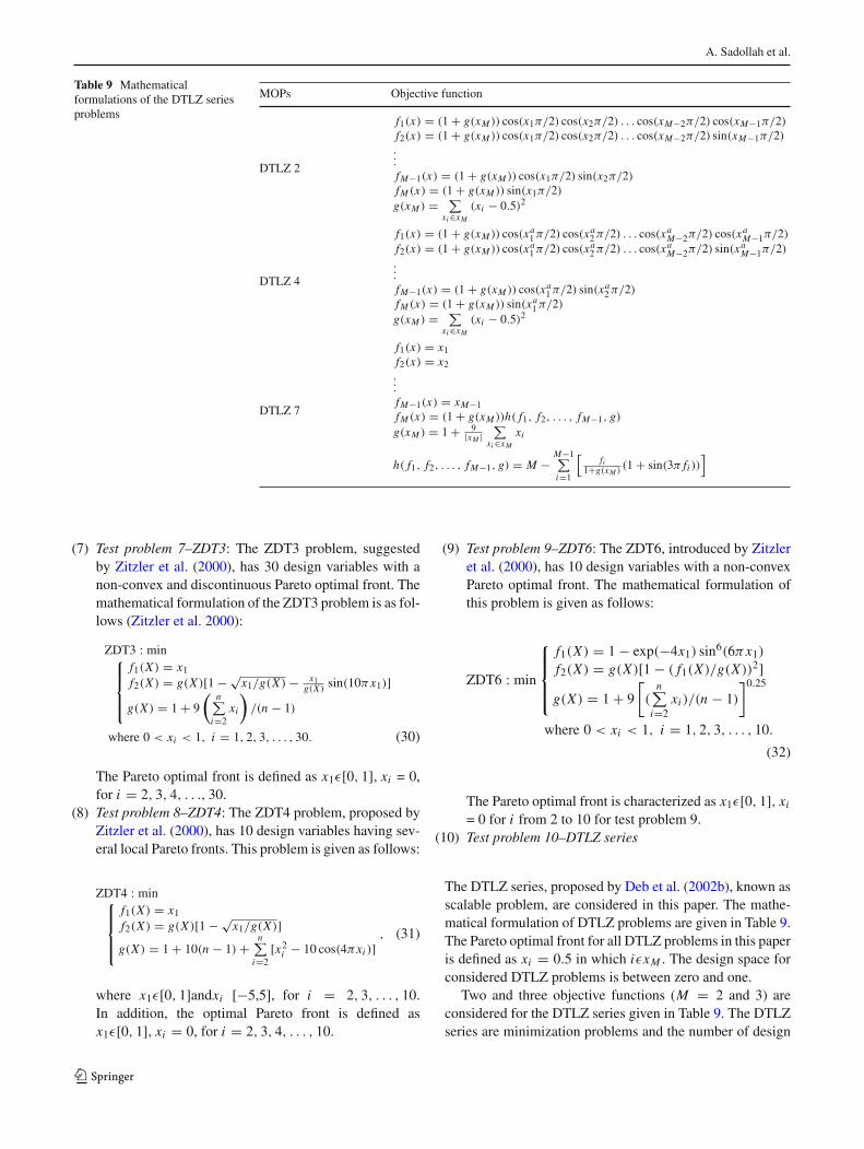
Table 9 Mathematicalformulations of the DTLZ seriesproblems

MOPs Objective function

DTLZ 2

f1(x) = (1 + g(xM )) cos(x1π/2) cos(x2π/2) . . . cos(xM−2π/2) cos(xM−1π/2)

f2(x) = (1 + g(xM )) cos(x1π/2) cos(x2π/2) . . . cos(xM−2π/2) sin(xM−1π/2)

.

.

.

fM−1(x) = (1 + g(xM )) cos(x1π/2) sin(x2π/2)

fM (x) = (1 + g(xM )) sin(x1π/2)

g(xM ) = ∑xi ∈xM

(xi − 0.5)2

DTLZ 4

f1(x) = (1 + g(xM )) cos(xa1 π/2) cos(xa

2 π/2) . . . cos(xaM−2π/2) cos(xa

M−1π/2)

f2(x) = (1 + g(xM )) cos(xa1 π/2) cos(xa

2 π/2) . . . cos(xaM−2π/2) sin(xa

M−1π/2)

.

.

.

fM−1(x) = (1 + g(xM )) cos(xa1 π/2) sin(xa

2 π/2)

fM (x) = (1 + g(xM )) sin(xa1 π/2)

g(xM ) = ∑xi ∈xM

(xi − 0.5)2

DTLZ 7

f1(x) = x1f2(x) = x2...

fM−1(x) = xM−1fM (x) = (1 + g(xM ))h( f1, f2, . . . , fM−1, g)

g(xM ) = 1 + 9|xM |

∑xi ∈xM

xi

h( f1, f2, . . . , fM−1, g) = M −M−1∑i=1

[fi

1+g(xM )(1 + sin(3π fi ))

]

(7) Test problem 7–ZDT3: The ZDT3 problem, suggestedby Zitzler et al. (2000), has 30 design variables with anon-convex and discontinuous Pareto optimal front. Themathematical formulation of the ZDT3 problem is as fol-lows (Zitzler et al. 2000):

ZDT3 : min⎧⎪⎪⎨

⎪⎪⎩

f1(X) = x1

f2(X) = g(X)[1 − √x1/g(X) − x1

g(X)sin(10πx1)]

g(X) = 1 + 9

(n∑

i=2xi

)/(n − 1)

where 0 < xi < 1, i = 1, 2, 3, . . . , 30. (30)

The Pareto optimal front is defined as x1ε[0, 1], xi = 0,for i = 2, 3, 4, . . ., 30.

(8) Test problem 8–ZDT4: The ZDT4 problem, proposed byZitzler et al. (2000), has 10 design variables having sev-eral local Pareto fronts. This problem is given as follows:

ZDT4 : min⎧⎪⎪⎨

⎪⎪⎩

f1(X) = x1

f2(X) = g(X)[1 − √x1/g(X)]

g(X) = 1 + 10(n − 1) +n∑

i=2[x2

i − 10 cos(4πxi )], (31)

where x1ε[0, 1]andxi [−5,5], for i = 2, 3, . . . , 10.In addition, the optimal Pareto front is defined asx1ε[0, 1], xi = 0, for i = 2, 3, 4, . . . , 10.

(9) Test problem 9–ZDT6: The ZDT6, introduced by Zitzleret al. (2000), has 10 design variables with a non-convexPareto optimal front. The mathematical formulation ofthis problem is given as follows:

ZDT6 : min

⎧⎪⎪⎨

⎪⎪⎩

f1(X) = 1 − exp(−4x1) sin6(6πx1)

f2(X) = g(X)[1 − ( f1(X)/g(X))2]g(X) = 1 + 9

[(

n∑i=2

xi )/(n − 1)

]0.25

where 0 < xi < 1, i = 1, 2, 3, . . . , 10.

(32)

The Pareto optimal front is characterized as x1ε[0, 1], xi

= 0 for i from 2 to 10 for test problem 9.(10) Test problem 10–DTLZ series

The DTLZ series, proposed by Deb et al. (2002b), known asscalable problem, are considered in this paper. The mathe-matical formulation of DTLZ problems are given in Table 9.The Pareto optimal front for all DTLZ problems in this paperis defined as xi = 0.5 in which iεxM . The design space forconsidered DTLZ problems is between zero and one.

Two and three objective functions (M = 2 and 3) areconsidered for the DTLZ series given in Table 9. The DTLZseries are minimization problems and the number of design

123

WCA for solving MOPs

variables for these problems is calculated as follows:

n = M + |xM | − 1, (33)

where n and M are the number of design variables and num-ber of objective functions, respectively. Also, |xM | is set to10 for all considered problems in this paper.

References

Atashpaz-Gargari E, Lucas C (2007) Imperialist competitive algorithm:an algorithm for optimization inspires by imperialistic competition.IEEE Congress on Evolutionary Computation, Singapore, pp 4661–4667

Blum C, Andrea R (2003) Metaheuristics in combinatorial optimiza-tion: overview and conceptual comparison. ACM Comput Surv35(3):268–308

Coello CAC, Lechuga MS (2002) MOPSO: A proposal for multi-ple objective particle swarm optimization. In: Proceedings of thecongress on evolutionary computation (CEC’2002), Honolulu, vo 1,pp1051–1056

Coello CAC (2000) An updated survey of GA-based multi-objectiveoptimization techniques. ACM Comput Surv 32(2):109–143

Coello CAC, Veldhuizen DAV, Lamont G (2002) Evolutionary algo-rithms for solving multi-objective problems., Genetic Algorithmsand Evolutionary ComputationKluwer, Dordrecht

Coello CAC (2004) Handling multiple objectives with particle swarmoptimization. IEEE T Evolut comput 8(3):256–279

Coello CAC, Cruz Cortés N (2005) Solving multiobjective optimizationproblems using an artificial immune system. Genet Program Evol M6:163–190

Deb K (2001) Multi-objective optimization using evolutionary algo-rithms. Wiley, New York

Deb K, Pratap A, Agarwal S, Meyarivan T (2002a) A fast and elitistmulti objective genetic algorithm: NSGA-II. IEEE Trans EvolutComput 6(2):182–197

Deb K (2002) Multi-objective genetic algorithms: problem difficultiesand construction of test problems. Evol Comput 7:205–230

Deb K, Thiele L, Laumanns M, Zitzler E (2002) Scalable multi-objective optimization test problems. In: Proceedings of IEEE Con-ference on Evolutionary Computation, pp 825–830

Eskandar H, Sadollah A, Bahreininejad A, Hamdi M (2012) Water cyclealgorithm—a novel metaheuristic optimization method for solvingconstrained engineering optimization problems. Comput Struct 110–111:151–166

Fonseca CM, Fleming PJ (1993) Genetic algorithms for multiobjectiveoptimization: formulation, discussion and generalization. In: ForrestS (ed) Proceedings of the fifth international conference on geneticalgorithms. Morgan Kauffman, San Mateo, pp 416–423

Freschi F, Repetto M (2006) VIS: an artificial immune network formulti-objective optimization. Eng Optim 38(8):975–996

Gao J, Wang J (2010) WBMOAIS: a novel artificial immune system formultiobjective optimization. Comput Oper Res 37:50–61

Glover FW, Kochenberger GA (2003) Handbook of metaheuristics.Kluwer, Dordrecht

Haupt RL, Haupt SE (2004) Practical genetic algorithms, 2nd edn. JohnWiley, New York

Holland J (1975) Adaptation in natural and artificial systems. Universityof Michigan Press, Ann Arbor

Kaveh A, Laknejadi K (2011) A novel hybrid charge system search andparticle swarm optimization method for multi-objective optimiza-tion. Expert Syst Appl 38(12):15475–15488

Kennedy J, Eberhart R (1995) Particle swarm optimization. In: Pro-ceedings of the IEEE international conference on neural networks.Perth, Australia, pp 1942–1948

Knowles JD, Corne DW (2000) Approximating the nondominated frontusing the Pareto archived evolution strategy. Evol Comput 8(2):149–172

Kursawe F (1991) A variant of evolution strategies for vector optimiza-tion. In: Lecture Notes in Computer Science. In: Proceedings of theParallel Problem Solving From Nature, PPSN I, vol 496, pp 193–197

Lin Q, Chen J (2013) A novel micro-population immune multiobjectiveoptimization algorithm. Comput Oper Res 40(6):1590–1601

Mahmoodabadi MJ, Adljooy Safaie A (2013) A novel combination ofparticle swarm optimization and genetic algorithm for pareto optimaldesign of a five-degree of freedom vehicle vibration model. Appl SoftComput 13:2577–2591

Mostaghim S, Teich J (2003) Strategies for finding good local guidesin multi objective particle swarm optimization (MOPSO). In: Pro-ceedings of the IEEE swarm intelligence symposium, pp 26–33

Osman IH, Laporte G (1996) Metaheuristics: a bibliography. Ann OperRes 63:513–623

Poloni C (1997) Hybrid GA for multiobjective aerodynamic shapeoptimization in genetic algorithms., Engineering and Computer Sci-enceWiley, New York

Pradhan PM, Panda G (2012) Solving multiobjective problems usingcat swarm optimization. Expert Syst Appl 39:2956–2964

Sierra MR, Coello CAC (2005) Improving PSO-based multi objectiveoptimization using crowding, mutation and e-dominance. In: Pro-ceedings of evolutionary multi-criterion optimization conference.Guanajuato, Mexico, pp 505–519

Srinivas N, Deb K (1995) Multi objective function optimization usingnondominated sorting genetic algorithms. Evol Comput 2(3):221–248

Viennet R, Fontiex C, Marc I (1995) New multicriteria optimizationmethod based on the use of a diploid genetic algorithm: example ofan industrial problem. In: Proceedings of Artificial Evolution. Brest,France, pp 120–127

Wang L, Zhong X, Liu M (2012) A novel group search optimizer formulti-objective optimization. Expert Syst Appl 39:2939–2946

Wang L, Zhong X, Liu M (2012) A novel group search optimizer formulti-objective optimization. Expert Syst Appl 39(3):2939–2946

Wang Y, Zeng J (2013) A multi-objective artificial physics optimizationalgorithm based on ranks of individuals. Soft Comput 17:939–952

Zhang B, Ren W, Zhao L, Deng X (2009) Immune system multiobjectiveoptimization algorithm for DTLZ problems. In: Fifth internationalconference on natural computation, pp 603–609

Zitzler E, Thiele L (1999) Multi objective evolutionary algorithms: acomparative case study and the strength Pareto approach. IEEE TransEvolut Comput 3(4):257–271

Zitzler E, Deb K, Thiele L (2000) Comparison of multi-objective evo-lutionary algorithms: empirical results. Evol Comput 8(2):173–195

Zitzler E, Laumanns M, Thiele L (2001) SPEA2: Improving the strengthPareto evolutionary algorithm. Swiss Federal Institute Technology,Zurich, Switzerland, TIK Report, vol 103, pp 1–21

123