a network simplex algorithm for solving the … · a network simplex algorithm for solving the...

JOURNAL OF INDUSTRIAL AND doi:10.3934/jimo.2009.5.929MANAGEMENT OPTIMIZATIONVolume 5, Number 4, November 2009 pp. 929–950

A NETWORK SIMPLEX ALGORITHM FOR SOLVING THEMINIMUM DISTRIBUTION COST PROBLEM

I-Lin Wang and Shiou-Jie Lin

Department of Industrial and Information ManagementNational Cheng Kung University

Tainan, 701, Taiwan

(Communicated by Shu-Cherng Fang)

Abstract. To model the distillation or decomposition of products in somemanufacturing processes, a minimum distribution cost problem (MDCP) fora specialized manufacturing network flow model has been investigated. Inan MDCP, a specialized node called a D-node is used to model a distillationprocess that connects with a single incoming arc and several outgoing arcs.The flow entering a D-node has to be distributed according to a pre-specifiedratio associated with each of its outgoing arcs. This proportional relationshipbetween arc flows associated with each D-node complicates the problem andmakes the MDCP more difficult to solve than a conventional minimum costnetwork flow problem. A network simplex algorithm for an uncapacitatedMDCP has been outlined in the literature. However, its detailed graphicalprocedures including the operations to obtain an initial basic feasible solution,to calculate or update the dual variables, and to pivot flows have never beenreported. In this paper, we resolve these issues and propose a modified networksimplex algorithm including detailed graphical operations in each elementaryprocedure. Our method not only deals with a capacitated MDCP, but alsooffers more theoretical insights into the mathematical properties of an MDCP.

1. Introduction. The minimum cost flow problem is a specialized linear program-ming problem with network structure which seeks an optimal flow assignment overa network satisfying the constraints of node flow balance and arc flow bounds (see[1]). However, these constraints are too simplified to model some real cases suchas, for example, the synthesis and distillation of products in some manufactur-ing processes. For this purpose, Fang and Qi [8] proposed a generalized networkmodel called the manufacturing network flow (MNF). The MNF considers threespecialized nodes: I-nodes, C-nodes, and D-nodes, to model the nodes of inven-tory, synthesis (combination), and distillation (decomposition), in addition to theconventional nodes: S-nodes, T-nodes, and O-nodes, which serve as sources, sinks,and transhipment nodes, respectively. Fang and Qi [8] also defined a minimumdistribution cost problem (MDCP) for a specialized MNF model referred to as thedistribution network which contains both D-nodes and conventional nodes. A D-node represents a distillation process and only connects with a single incoming arc

2000 Mathematics Subject Classification. Primary: 90B10, 05C85; Secondary: 05C21.Key words and phrases. network optimization, manufacturing network, distribution network,

minimum distribution cost flow problem, network simplex algorithm.I-Lin Wang was partially supported by the National Science Council of Taiwan under Grant

NSC95-2221-E-006-268.

929

http://dx.doi.org/10.3934/jimo.2009.5.929

930 I-LIN WANG AND SHIOU-JIE LIN

M

T1

T2

T3

[0.2]

[0.8]

( )object,cost,capacity

[ ]material composition percentage

( )A,3,30

( )A,4,40

( )A,2,40

( )A,5,50

( )A,3,30

( )B,3,20

( )C,3,30

( )B,2,20

( )C,4,30

( )B,3,40

( )B,4,10

( )C,3,20

( )B,4,50

( )C,3,30

( )A,1,20

( )A,5,50

d i i= the demand of T

d1=10

d2=20

d3=20

[0.2]

[0.8]

( )A,5,70

Figure 1. An MDCP example in a supply chain network

and several outgoing arcs. The flows passing through a D-node have to satisfy theflow distillation constraint. This constraint requires the flows entering a D-node tobe distributed to each of its outgoing arcs called distillation arcs, according to apre-specified ratio associated with each outgoing arc. For each D-node i with enter-ing flow xi∗i on its incoming arc (i∗, i), the flow distillation constraint specifies theflow on its distillation arc (i, j) to be xij = kijxi∗i where kij is a constant between0 and 1 and

∑(i,j) kij = 1.

The MDCP can appear often in part of a supply chain network. Take Figure1 as a reverse logistics network example. A recycled product collecting site Mdistributes a recycled product A which then will be decomposed (or distilled) intomaterials B and C in two different recycle plants (half-circled nodes), and finallytransported to landfills T1, T2 , and T3. In this example, each recycle plant is aD-node; M is the S-node; T1, T2, and T3 are the T-nodes; and all the other nodesare O-nodes. Suppose that each recycle plant can decompose one unit of A into 0.2unit of B and 0.8 unit of C. Each arc in the reverse logistics network in Figure 1represents some operation (e.g. transportation) associated with a unit cost as wellas a capacity constraint. The MDCP in Figure 1 seeks the minimum possible totalcost to satisfy the demand requirements of landfills T1, T2, and T3.

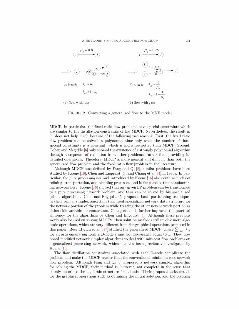
At first glance, the MDCP seems similar to the generalized network flow problemwhere the flow along an arc (i, j) may lose or gain based on a gain factor µij , definedas the ratio of the flow arriving at the head node j to the flow leaving from thetail node i. In fact, the generalized flow problem is a special case of the MDCPmodel. Take Figure 2(a) as an example. For each arc (i, j) with loss of flows (i.e.µij < 1), one may convert it to an MDCP model by adding a dummy sink arc (i, j′)and a D-node α where the flow distillation factors kαj and kαj′ can be derived fromµij . Similarly, one may also convert each arc with the gain of flows to an MNFmodel by adding a dummy source arc and a C-node (see Figure 2(b) for details).Besides the generalized flow problem, Cohen and Megiddo [6] also discussed a classof parametric flow problems in which the fixed ratio flow problem is similar to the

A NETWORK SIMPLEX ALGORITHM FOR MDCP 931

i ij j

i

j'

j ij

i'

α β

0.8

0.2

0.8

0.2

α: D-node β: C-node

(a) flow with loss (b) flow with gain

Figure 2. Converting a generalized flow to the MNF model

MDCP. In particular, the fixed-ratio flow problems have special constraints whichare similar to the distillation constraints of the MDCP. Nevertheless, the result in[6] does not help much because of the following two reasons: First, the fixed ratioflow problem can be solved in polynomial time only when the number of thosespecial constraints is a constant, which is more restrictive than MDCP; Second,Cohen and Megiddo [6] only showed the existence of a strongly polynomial algorithmthrough a sequence of reduction from other problems, rather than providing itsdetailed operations. Therefore, MDCP is more general and difficult than both thegeneralized flow problem and the fixed ratio flow problem in the literature.

Although MDCP was defined by Fang and Qi [8], similar problems have beenstudied by Koene [16], Chen and Engquist [5], and Chang et al. [4] in 1980s. In par-ticular, the pure processing network introduced by Koene [16] also contains nodes ofrefining, transportation, and blending processes, and is the same as the manufactur-ing network here. Koene [16] showed that any given LP problem can be transformedto a pure processing network problem, and thus can be solved by his specializedprimal algorithms. Chen and Engquist [5] proposed basis partitioning techniquesin their primal simplex algorithm that used specialized network data structure forthe network portion of the problem while treating the other non-network portion aseither side variables or constraints. Chang et al. [4] further improved the practicalefficiency for the algorithms by Chen and Engquist [5]. Although these previousworks also focused on solving MDCPs, their solution methods still involve more alge-braic operations, which are very different from the graphical operations proposed inthis paper. Recently, Lu et al. [17] studied the generalized MDCP, where

∑(i,j) kij

for all arcs emanating from a D-node i may not necessarily equal to 1. They pro-posed modified network simplex algorithms to deal with min-cost flow problems ona generalized processing network, which has also been previously investigated byKoene [16].

The flow distillation constraints associated with each D-node complicate theproblem and make the MDCP harder than the conventional minimum cost networkflow problem. Although Fang and Qi [8] proposed a network simplex algorithmfor solving the MDCP, their method is, however, not complete in the sense thatit only describes the algebraic structure for a basis. Their proposal lacks detailsfor the graphical operations such as obtaining the initial solution, and the pivoting


and updating procedures for both the arc flows and node potentials. This paper re-solves these issues and proposes a network simplex algorithm with detailed graphicaloperations for solving an MDCP.

In addition to the MDCP, Fang and Qi [8] also introduced a max-flow prob-lem for a distribution network, but they did not propose any method to solve theproblem. Sheu et al. [19] proposed a multi-labelling method to solve this problemby adopting the concept of the augmenting path method [9] and the Depth-FirstSearch algorithm (DFS) which tries every augmenting subgraph that goes to thesink or source and satisfies the flow distillation constraints. After finding such anaugmenting subgraph, the algorithm then identifies decomposable components inan augmenting subgraph where the flow inside each component can be representedby a single variable. The flow can be calculated by the flow balance constraints forall nodes that joint different components. Although this method is straightforward,its complexity is shown to be non-polynomial.

Wang and Lin [21] proposed compacting rules and a polynomial-time compactingalgorithm which can serve as a preprocessing procedure to simplify the MDCPproblem structure. Specifically, a group of connected D-nodes can be shrunk into asingle D-node. Any transhipment O-node with single incoming and outgoing arcscan be transformed into a single arc. Capacities on arcs connecting with a D-nodecan be unified using the same standards by its flow distillation constraints. Afterconducting their polynomial-time compacting procedures, the original network willbe compacted to an equivalent one of smaller size.

Wang and Yang [22] solved three specialized uncapacitated MDCPs: UMDCP1,UMDCP2, and UMDCP3 based on Dijkstra’s algorithm [7]. Other network com-pacting rules which unify the effects of arc costs have also been proposed by the sameauthor. Although two algorithms modified from the Dijkstra’s algorithm have beendesigned to solve UMDCP1 and UMDCP2, they can not efficiently solve UMDCP3.

A multicommodity MNF model of σ + 1 commodities was investigated by Mo etal. [18], in which there are σ + 1 layers with each layer corresponding to a networkof the same commodity with inter-layer arcs connecting C-nodes or D-nodes. Theirmodel is more restrictive and simplified in the sense that: First, it is assumed thatthere is only one kind of D-node to decompose commodity 0 into η commoditiesand one kind of C-node to combine commodity σ from λ commodities; Second,the distillation factor k associated with each D-node (or C-node) is assumed to beidentical (i.e. k = 1/η for a D-node, or k = 1/λ for a C-node). Moreover, theelementary procedures in their proposed network simplex algorithm are still purealgebraic rather than graphical operations.

Among all the related literatures, the network-simplex-based solution method byVenkateshan et al. [20] discussed more graphical data structures and operations forsolving min-cost MNF problems. Their works are similar to this paper, but theiralgorithm and notations were not clearly presented. On the other hand, we givemore detailed and clear graphical illustration on the theoretical characteristics andcomplexity for each step of our network simplex algorithm.

In short, several specialized MDCPs have been solved in the literature, yet theirproblems are more restrictive (e.g. [18], [21], [22], [19]) or lack graphical operations(e.g. [16], [5], [4], [8], [18]). Since a network simplex algorithm should contain moregraphical operations than pure algebraic operations like the conventional simplexalgorithm, we propose here in this paper the detailed graphical operations for eachelementary procedure in a network simplex algorithm for solving the MDCP. Our


Figure 3. S-node, T-node, O-node and D-node

work provides a more efficient graphical implementation and more insights into thesolution structures. The techniques developed in this paper can also be used tosolve the problems in [19] and [22].

The rest of this paper is organized as follows: Section 2 introduces definitionsand notations, presents a model transformation for easier illustration, defines abasic feasible graph, and provides optimality conditions for our network simplexalgorithm. Detailed procedures of our network simplex algorithm are illustrated inSection 3. Finally, Section 4 summarizes and concludes the paper.

2. Preliminaries.

2.1. Notations and model transformation. Let G = (N, A) be a directed sim-ple graph with node set N and arc set A. For each arc (i, j) ∈ A, we associate itwith a unit flow cost cij and a flow capacity uij where the arc flow xij ∈ [0, uij ].For each node i ∈ N , we define the set of nodes connecting to and from it asE(i) := {j ∈ N : (j, i) ∈ A} and L(i) := {j ∈ N : (i, j) ∈ A}, respectively. Thereare four kinds of nodes (see Figure 3): S-nodes, T-nodes, O-nodes, and D-nodes,and they are denoted by NS , NT , NO, and ND, respectively. An S-node is a sourcenode connected only by outgoing arcs. A T-node denotes a sink node connectedonly by incoming arcs. An O-node represents a transshipment node connected withboth incoming and outgoing arcs. Usually, an S-node is a supply node, a T-node isa demand node, and an O-node is for transshipment. We refer to these three typesof nodes as conventional nodes since they only have to satisfy the flow balanceconstraints. A D-node connects with one incoming arc and at least two outgoingarcs. For each node i ∈ ND with incoming arc (i∗, i), the flow distillation constraintspecifies xij = kijxi∗i for the flow on its distillation arc (i, j). Furthermore, we as-sume

∑j∈L(i) kij = 1 in order to satisfy the flow balance constraint. Without loss

of generality, we assume all the networks in this paper to have already been com-pacted using the rules and algorithms by Wang and Lin [21] and Wang and Yang[22]. Also, we assume that the MDCP problem contains a finite optimal solution.

Shipping flows from several S-nodes to several T-nodes through O-nodes andD-nodes, an MDCP model proposed by Fang and Qi [8] is defined as follows:

min∑

i∈NS

cixi +∑

(i,j)∈A

cijxij (MDCPFQ)

s.t.∑

j∈L(i)

xij − xi = 0 ∀i ∈ NS (1)


xj −∑

i∈E(j)

xij = 0 ∀j ∈ NT (2)

∑

j∈L(i)

xij − xi∗i = 0 ∀i ∈ ND, (i∗, i) ∈ A (3)

xij − kijxi∗i = 0 ∀i ∈ ND, (i∗, i) ∈ A, (i, j) ∈ A (4)

xi ≤ ui ∀i ∈ NS (5)

0 ≤xij ≤ uij ∀(i, j) ∈ A (6)

where ui for each i ∈ NS represents the maximum possible flow that a source nodei receives for shipping out, dj for each node j ∈ NT denotes the minimum amountof flow that a sink node has to receive, and

∑i∈NS

ui ≥∑

j∈NTdj .

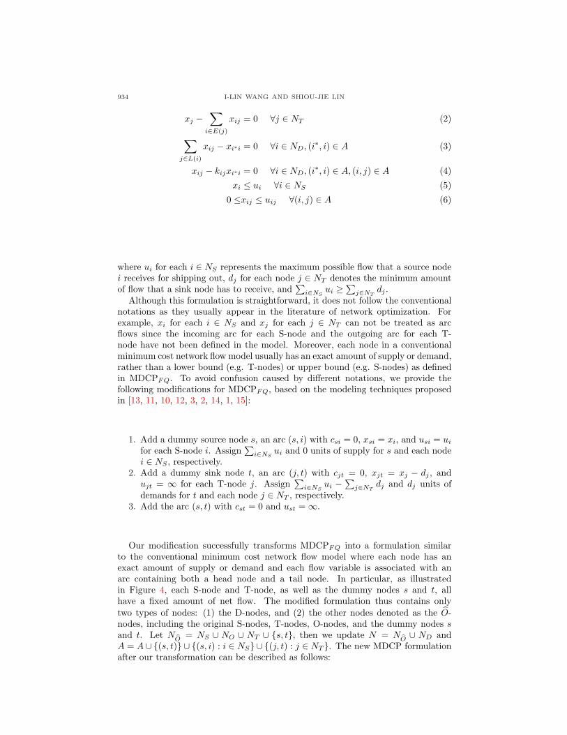
Although this formulation is straightforward, it does not follow the conventionalnotations as they usually appear in the literature of network optimization. Forexample, xi for each i ∈ NS and xj for each j ∈ NT can not be treated as arcflows since the incoming arc for each S-node and the outgoing arc for each T-node have not been defined in the model. Moreover, each node in a conventionalminimum cost network flow model usually has an exact amount of supply or demand,rather than a lower bound (e.g. T-nodes) or upper bound (e.g. S-nodes) as definedin MDCPFQ. To avoid confusion caused by different notations, we provide thefollowing modifications for MDCPFQ, based on the modeling techniques proposedin [13, 11, 10, 12, 3, 2, 14, 1, 15]:

1. Add a dummy source node s, an arc (s, i) with csi = 0, xsi = xi, and usi = ui

for each S-node i. Assign∑

i∈NSui and 0 units of supply for s and each node

i ∈ NS , respectively.2. Add a dummy sink node t, an arc (j, t) with cjt = 0, xjt = xj − dj , and

ujt = ∞ for each T-node j. Assign∑

i∈NSui −

∑j∈NT

dj and dj units ofdemands for t and each node j ∈ NT , respectively.

3. Add the arc (s, t) with cst = 0 and ust = ∞.

Our modification successfully transforms MDCPFQ into a formulation similarto the conventional minimum cost network flow model where each node has anexact amount of supply or demand and each flow variable is associated with anarc containing both a head node and a tail node. In particular, as illustratedin Figure 4, each S-node and T-node, as well as the dummy nodes s and t, allhave a fixed amount of net flow. The modified formulation thus contains onlytwo types of nodes: (1) the D-nodes, and (2) the other nodes denoted as the O-nodes, including the original S-nodes, T-nodes, O-nodes, and the dummy nodes sand t. Let NO = NS ∪ NO ∪ NT ∪ {s, t}, then we update N = NO ∪ ND andA = A ∪ {(s, t)} ∪ {(s, i) : i ∈ NS} ∪ {(j, t) : j ∈ NT }. The new MDCP formulationafter our transformation can be described as follows:


s

i

ui

ui

i

[ - ]i

i

S

[ ]-di

t

Figure 4. Transforming the MDCPFQ to the conventional mini-mum cost network flow model

min∑

(i,j)∈A

cijxij (MDCP)

s.t. xst +∑

i∈NS

xsi =∑

i∈NS

ui for s (7)

xsi −∑

j∈L(i)

xij = 0 ∀i ∈ NS (8)

∑

j∈L(i)

xij −∑

j∈E(i)

xij = 0 ∀i ∈ NO (9)

xjt −∑

i∈E(j)

xij = −dj ∀j ∈ NT (10)

−xst −∑

j∈NT

xjt =∑

j∈NT

dj −∑

i∈NS

ui for t (11)

∑

j∈L(i)

xij −∑

j∈E(i)

xij = 0 ∀j ∈ ND (12)

kijxi∗i − xij = 0 ∀i ∈ ND, (i∗, i) ∈ A, (i, j) ∈ A (13)

0 ≤ xij ≤ uij ∀(i, j) ∈ A (14)

where equations (7) to (12) define the flow balance for each node in N , equation(13) is the flow distillation constraint associated with each D-node, and equation(14) defines the arc flow bounds. Note that we assume

∑j∈L(i) kij = 1 which

means that equation (12) can be derived from equation (13) and thus equation(12) is removable. This new formulation has several advantages. First, it treats


the MDCP as a side-constrained minimum cost network flow problem where onlya new set of flow distillation constraints (i.e. equations (13)) are added in additionto the conventional flow balance and bound constraints; Second, the basic graphcorresponding to the basis is connected. Furthermore, the connectivity property ofthe basic graph is helpful in the development of our network simplex algorithm.

2.2. Basic feasible graph. In a conventional minimum cost network flow prob-lem, a basis corresponds to a spanning tree so that the network simplex algorithmcan easily operate from one spanning tree to another. Here in MDCP, the basiscorresponding to a basic feasible flow x constitutes a subgraph GB(x) composedby a spanning tree and some distillation arcs. Since the flow balance constraintsin MDCP are the same as the conventional minimum cost network flow problem,GB(x) at least contains a spanning tree of n−1 basic arcs derivable from equations(7) to (12). Suppose each D-node i contains qi distillation arcs, q =

∑i∈ND

qi,and that there are a total of p D-nodes. Since equation (12) can be derived fromequation (13), we can remove equation (12) and then the rank of the constraints(7) to (13) equals to n + q − p − 1 since there are a total of p D-nodes. The basicfeasible graph for an MDCP has the following properties:

Lemma 2.1. Let x be a basic feasible solution of an MDCP and GB(x) be the basicfeasible graph corresponding to x, where |N | = n, |ND| = p, |L(i)| = qi for eachi ∈ ND and q =

∑i∈ND

qi. The basic graph has the following properties:(i) The number of basic arcs is n + q − p− 1.(ii) Any cycle of GB(x) includes at least one D-node.(iii) GB(x) is connected.(iv) Each D-node i is connected with qi or qi + 1 basic arcs.(v) After removing qi − 1 basic arcs for each D-node i, GB(x) can be reduced to aspanning tree.

Proof. (i) Trivial.(ii) See [8].(iii) Our MDCP contains the same flow balance constraints corresponding to aconnected spanning tree, as in the conventional minimum cost flow problem. Thusthe basic graph of our MDCP is connected.(iv) See [8].(v) The proof is modified from [8]. By (iii), we know that any cycle in GB(x) passesat least one D-node. Since each D-node i is connected by at least qi arcs by (iv),and if we remove qi − 1 basic arcs for each D-node i (i.e., totally removing q − parcs) from GB(x), then the remaining basic graph contains n − 1 basic arcs andremains connected without any cycle which corresponds to a spanning tree.

Although our Lemma 2.1 seems similar to the properties proposed by Fang andQi [8], they are not identical in the following sense: First, we generalized theirresults to deal with a capacitated MDCP whereas their results are only applicablefor an uncapacitated MDCP; Second, we suggest a more specific way (property(v) in Lemma 2.1) to describe the relationship between GB(x) and its inducedspanning tree, which helps us to design the optimality conditions in Section 2.3 andour graphical network simplex algorithm in Section 3.


2.3. Dual variables and optimality conditions. Let πi and πi be dual variablesassociated with the flow balance constraint for each node i ∈ NO (equation (7)to (11)) and i ∈ ND (equation (12)), respectively. Let vij denote dual variableassociated with the flow distillation constraint (equation (13)) for each distillationarc (i, j). The constraints of the dual problem of an MDCP can be formulated asfollows:

πi − πj ≤ cij ∀i, j ∈ NO (15)

πi − vij − πj ≤ cij ∀i ∈ ND, j ∈ NO (16)

πi − πj +∑

l∈L(j)

kjlvjl ≤ cij ∀j ∈ ND, i ∈ E(j) (17)

For each distillation arc (j, l) leaving D-node j, define ρjl = πj − vjl and πj =∑l∈L(j) kjlρjl . Since

∑l∈L(j) kjl = 1, we will have πj −

∑l∈L(j) kjlvjl =

∑l∈L(j)

kjl(πj − vjl) =∑

l∈L(j) kjlρjl = πj . Equation (15) to (17) can be rewritten as

πi − πj ≤ cij ∀i ∈ NO, j ∈ N (18)

ρij − πj ≤ cij ∀i ∈ ND, j ∈ NO (19)

We apply the upper bound technique for linear programming to solve a capac-itated MDCP. Specifically, when xij = uij for an arc (i, j), one may consider itsorientation to be reversed. This also means that the check on its dual feasibilityconstraint has to be conducted conversely (e.g. replace the ≤ with ≥ in equations(18) and (19)). The upper bound technique can also be implemented in the originalmodel proposed by Fang and Qi [8], but their basic graph can not be guaranteed tobe connected, which complicates the procedure to traverse along arcs for checkingthe dual feasibility. On the other hand, the basic graph is shown to be connectedin our model by Lemma 2.1(iii).

Let B, L, and U be the set of basic arcs, non-basic arcs at lower bound, andnon-basic arcs at upper bound, respectively. Thus the set of all arcs A = B∪L∪U .The dual optimality conditions are then as follows:

1. For each arc (i, j) ∈ B,

πi − πj = cij ∀i ∈ NO, j ∈ N (20)

ρij − πj = cij ∀i ∈ ND, j ∈ NO (21)

2. For each arc (i, j) ∈ L,

πi − πj ≤ cij ∀i ∈ NO, j ∈ N (22)

ρij − πj ≤ cij ∀i ∈ ND, j ∈ NO (23)

3. For each arc (i, j) ∈ U ,

πi − πj ≥ cij ∀i ∈ NO, j ∈ N (24)

ρij − πj ≥ cij ∀i ∈ ND, j ∈ NO (25)

3. Network Simplex algorithm. The network simplex algorithm is a specializedsimplex algorithm designed specifically for solving network-type linear programmingproblems. The conventional network simplex algorithm is designed for minimumcost network flow problem and exploits graphical operations in order to efficientlycalculate the basic feasible solutions. However, it cannot deal with the distillation


constraints of an MDCP. On the other hand, the network simplex algorithm pro-posed by Fang and Qi [8] for an MDCP is not complete in the sense that many stepsin their algorithm are only algebraic operations. To fully exploit the advantage ofgraphical operations, we propose a network simplex algorithm including technicaldetails in such steps as to allow us to obtain the initial basic feasible solutions, topivot flows along basic feasible graphs, and to update dual basic solutions for solvinga capacitated MDCP. Without loss of generality, we assume that our MDCP alwayshas a finite optimal solution and that the degeneracy is resolved using anti-cyclingtechniques. Our network simplex algorithm contains the following steps:

Step 0: Start with an initial basic feasible flow on a basic feasible graph GB(x).Step 1: Calculate dual basic solutions for GB(x).Step 2: Check the dual feasibility conditions (equation (22) to (25)) for each arc in

L∪U . If no arcs violate the optimality conditions, then the flow x is optimaland the algorithm terminates.Otherwise, select a violating arc (k, l) as the entering arc to the basis andcontinue Step 3.

Step 3: Conduct flow pivoting operations and determine the leaving arc (v, z).Step 4: Update dual variables, and then return to Step 2 for the next iteration.

Our algorithm exploits several novel basis partitioning techniques which decom-pose a basic graph into components so that arc flows as well as node potentialscan be efficiently calculated and updated. Detailed operations for each step areexplained in the next sections.

3.1. Obtaining an initial basic feasible flow. Let M be a very large number.We present the following procedure based on the Big-M method to compute aninitial basic feasible flow:

Step 1: For each i ∈ NS , include arc (s, i) into the basis with xsi := 0. Alsoinclude arc (s, t) into the basis with xst :=

∑i∈NS

ui −∑

i∈NTdj .

Step 2: For each i ∈ NO, add artificial arcs (s, i) to be a basic arc with usi := M ,csi := M , and xsi := 0.

Step 3: For each i ∈ NT , add artificial arcs (s, i) to be a basic arc with usi := M ,csi := M , and xsi := di.

Step 4: For each i ∈ ND, include each distillation arc (i, j) where j ∈ L(i) to be abasic arc with xij := 0.

In particular, Step 1 through Step 3 identify n − p − 1 basic arcs, and Step 4identifies another basic arcs. The flow assignments are feasible since all the supplyand demand are satisfied. Furthermore, basic dual variables can be calculated bysetting πs := 0, πi := −csi for each i ∈ NO, ρij := πj + cij for each distillation arc(i, j), and πi :=

∑j∈L(i) kijρij for each i ∈ ND. This procedure takes O(n + q − p)

time.

3.2. Calculating basic dual solutions. Fang and Qi [8] outlined this procedurewithout detailed graphical implementation. In the present paper we propose a basispartitioning technique that decomposes the basic graph into p+1 basic components,in which each basic component is a tree and contains at least one D-node or onedistillation arc. We show that all dual variables on the same basic component can


i

j

j

i

i

Figure 5. Detaching the distillation from a D-node

be expressed using a representative dual variable (e.g. the π associated with somenode in that basic component) due to its tree structure, so that we can use the p+1representative dual variables to derive all the n+q dual variables. A system of p+1linear equations, composed by πi = ς for some node i ∈ N or ραβ = ς for somedistillation arc (α, β) with a constant ς, as well as p equations πi =

∑j∈L(i) kijρij

of for each i ∈ ND, can be used to solve the p+1 representative dual variables, andthen to derive all the n + q dual variables.

3.2.1. Decomposing the Basic Graph into Basic Components. When solving basicdual variables for a minimum cost network flow problem, the network simplex al-gorithm starts from any node i, sets πi to be a fixed value ς (e.g. ς = 0), andthen calculates other dual variables by tracing basic arcs along the basic tree arcs.Here in MDCP, such a tracing operation is not trivial when a D-node is encoun-tered. Specifically, when starting from a node i ∈ N one may trace along basic arcsand calculate other dual variables π or ρ using equations (20) and (21). However,when a D-node i is encountered, the tracing has to be stopped since the qi + 1 dualvariables in the equation πi =

∑j∈L(i) kijρij associated with a D-node i cannot be

calculated using a single equation (i.e. equation (20) or (21)). A search algorithmsuch as the Depth-First Search (DFS) or Breadth-First-Search (BFS) can be usedto trace the basic arcs and calculate dual variables using equation (20) and (21), aslong as we do not crossover a D-node. Once the search algorithm backtracks to itsstarting node it can start from any unvisited node and conduct the same operationsuntil all the nodes in N have been visited. That is to say , D-nodes can be viewedas boundary nodes for the search algorithm.

To have a better illustration for this operation, we detach each distillation arc(i, j) outgoing from each D-node i, and replace its tail node by a pseudo node ijreferred to as a side-node (the squared nodes in Figure 5). A new dual variableπij = ρij is assigned to the side-node ij for recording dual variable ρij associatedwith the distillation arc (i, j). Thus equation (21) becomes πij− πj = cij for eachdistillation basic arc (i, j) and has a form similar to equation (20). Now we onlyneed to consider dual variables π associated with each node in N and each side-node.

The detachment procedure disconnects each D-node i and all the nodes it em-anates to. By lemma 2.1(iv), we know that each D-node i is connected by either qi

or qi+1 basic arcs. Lemma 2.1(v) also suggests that the disconnection of qi−1 basicarcs for each D-node i in GB(x) reduces the GB(x) to a spanning tree, denoted asT (x). Therefore, the disconnection of qi basic arcs for each D-node i in GB(x) willdisconnect one more basic arc for each D-node i in the spanning tree T (x). Since


47

48

46

56

59

BC2

BC1

BC3

BC1

BC3

BC2

Figure 6. An example of basic components

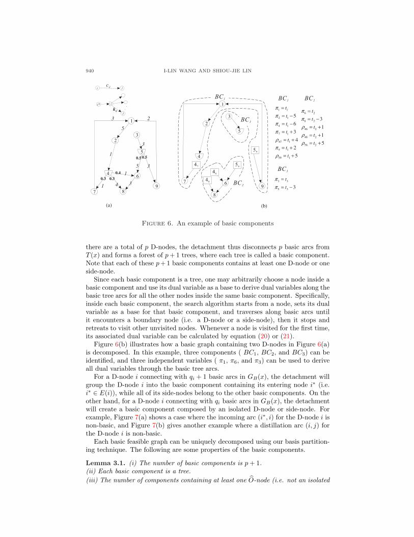
there are a total of p D-nodes, the detachment thus disconnects p basic arcs fromT (x) and forms a forest of p + 1 trees, where each tree is called a basic component.Note that each of these p+1 basic components contains at least one D-node or oneside-node.

Since each basic component is a tree, one may arbitrarily choose a node inside abasic component and use its dual variable as a base to derive dual variables along thebasic tree arcs for all the other nodes inside the same basic component. Specifically,inside each basic component, the search algorithm starts from a node, sets its dualvariable as a base for that basic component, and traverses along basic arcs untilit encounters a boundary node (i.e. a D-node or a side-node), then it stops andretreats to visit other unvisited nodes. Whenever a node is visited for the first time,its associated dual variable can be calculated by equation (20) or (21).

Figure 6(b) illustrates how a basic graph containing two D-nodes in Figure 6(a)is decomposed. In this example, three components ( BC1, BC2, and BC3) can beidentified, and three independent variables ( π1, π6, and π3) can be used to deriveall dual variables through the basic tree arcs.

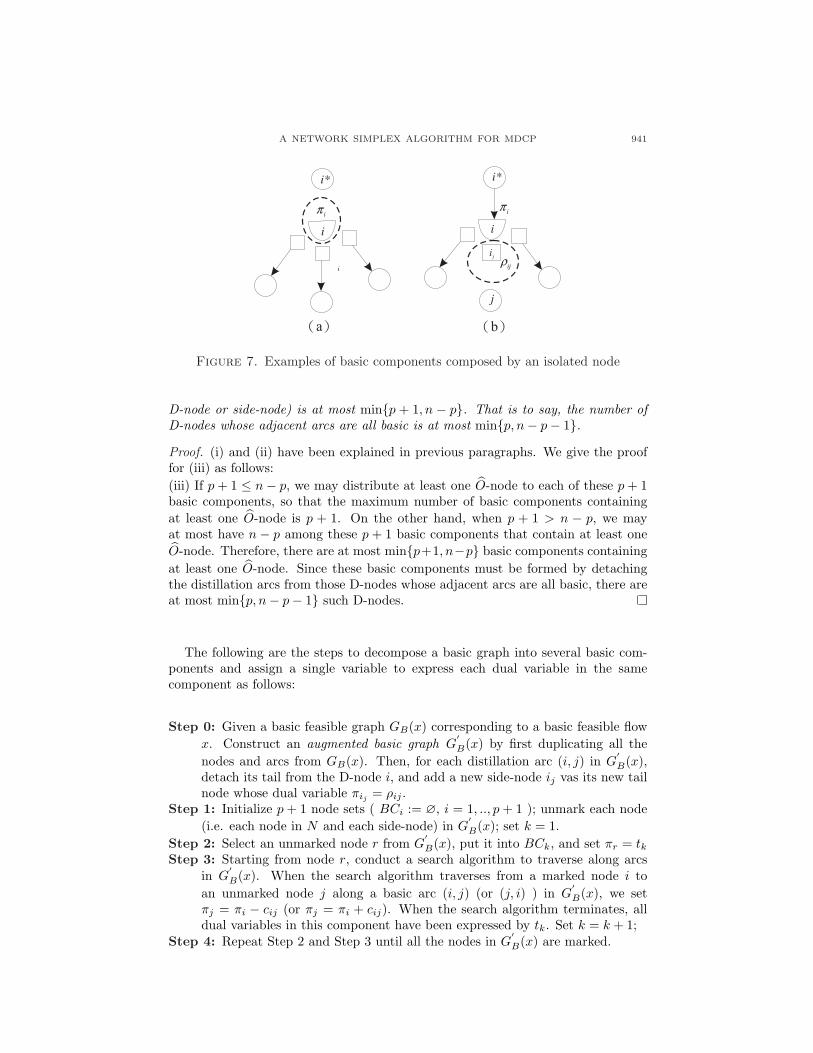
For a D-node i connecting with qi + 1 basic arcs in GB(x), the detachment willgroup the D-node i into the basic component containing its entering node i∗ (i.e.i∗ ∈ E(i)), while all of its side-nodes belong to the other basic components. On theother hand, for a D-node i connecting with qi basic arcs in GB(x), the detachmentwill create a basic component composed by an isolated D-node or side-node. Forexample, Figure 7(a) shows a case where the incoming arc (i∗, i) for the D-node i isnon-basic, and Figure 7(b) gives another example where a distillation arc (i, j) forthe D-node i is non-basic.

Each basic feasible graph can be uniquely decomposed using our basis partition-ing technique. The following are some properties of the basic components.

Lemma 3.1. (i) The number of basic components is p + 1.(ii) Each basic component is a tree.(iii) The number of components containing at least one O-node (i.e. not an isolated


i j

( )a ( )b

Figure 7. Examples of basic components composed by an isolated node

D-node or side-node) is at most min{p + 1, n − p}. That is to say, the number ofD-nodes whose adjacent arcs are all basic is at most min{p, n− p− 1}.Proof. (i) and (ii) have been explained in previous paragraphs. We give the prooffor (iii) as follows:(iii) If p + 1 ≤ n− p, we may distribute at least one O-node to each of these p + 1basic components, so that the maximum number of basic components containingat least one O-node is p + 1. On the other hand, when p + 1 > n − p, we mayat most have n − p among these p + 1 basic components that contain at least oneO-node. Therefore, there are at most min{p+1, n−p} basic components containingat least one O-node. Since these basic components must be formed by detachingthe distillation arcs from those D-nodes whose adjacent arcs are all basic, there areat most min{p, n− p− 1} such D-nodes.

The following are the steps to decompose a basic graph into several basic com-ponents and assign a single variable to express each dual variable in the samecomponent as follows:

Step 0: Given a basic feasible graph GB(x) corresponding to a basic feasible flowx. Construct an augmented basic graph G

′B(x) by first duplicating all the

nodes and arcs from GB(x). Then, for each distillation arc (i, j) in G′B(x),

detach its tail from the D-node i, and add a new side-node ij vas its new tailnode whose dual variable πij = ρij .

Step 1: Initialize p + 1 node sets ( BCi := ∅, i = 1, .., p + 1 ); unmark each node(i.e. each node in N and each side-node) in G

′B(x); set k = 1.

Step 2: Select an unmarked node r from G′B(x), put it into BCk, and set πr = tk

Step 3: Starting from node r, conduct a search algorithm to traverse along arcsin G

′B(x). When the search algorithm traverses from a marked node i to

an unmarked node j along a basic arc (i, j) (or (j, i) ) in G′B(x), we set

πj = πi − cij (or πj = πi + cij). When the search algorithm terminates, alldual variables in this component have been expressed by tk. Set k = k + 1;

Step 4: Repeat Step 2 and Step 3 until all the nodes in G′B(x) are marked.


Note that the augmented basic graph G′B(x) contains n+q−p−1 basic arcs and

n + q nodes. The search algorithm scans each arc and node exactly once in Step 3and results in a total θ(n + q) time for this procedure.

3.2.2. Solving a Smaller System of Linear Equations. After decomposing the p + 1basic components, dual variable associated with each node inside the basic compo-nent has been expressed using the representative variable ti. Thus, there are a totalof p + 1 representative dual variables. Similar to the conventional network simplexalgorithm for the minimum cost flow problem where one can arbitrarily set a dualvariable to a fixed value and then derive all other dual variables with respect tothat dual variable via basic arcs, here we can also arbitrarily select a dual variableas a base and compute all other p dual variables accordingly. For example, settingπ1 = t1 = 0, we will have p representative variables (ti : i = 2, ..., p + 1) and asystem of p linear equations (πi =

∑j∈L(i) kijρij : i ∈ ND).

Take Figure 6 as an example. Using π1 = 0 and the relations between dualvariables as defined in Figure 6(b), the equations associated with flow distillationconstraints: π4 = 0.4ρ46 +0.3ρ47 +0.3ρ48 and π5 = 0.5ρ56 +0.5ρ59 can be expressedusing t2 and t3, and we can compute t2 = −11.286 and t3 = 0.5t2 + 8 = 2.357.

Although our basis partitioning technique requires us to solve a system of plinear equations for calculating basic dual variables, this is already more efficientthan solving a system of n + q − p − 1 linear equations as required in the networksimplex method proposed by Fang and Qi [8]. In fact, the efficiency of our methodcan be improved further, if a better ordering in the sequence of components to besolved can be identified. For example, in Figure 6(b), D-node 4 is the boundarynode for two components (BC1 and BC2), and D-node 5 is the boundary nodefor three components (BC1, BC2, and BC3). Setting t3 = 0 will have to solve a2 × 2 system of linear equations, whereas setting t1 = 0 or t2 = 0 will make theremaining system of linear equations become a triangular form, which can be solvedmore efficiently.

To speed up this procedure, we may reduce the number of linear equations re-quired to be solved. We first identify the following three types of basic components:(1) a basic component composed of an isolated D-node or side-node (e.g. Figure7), (2) a basic component that contains exactly one D-node, some O-nodes but noside-nodes (e.g. the BC3 in Figure 6), and (3) a basic component that contains noD-node, some O-nodes, and some side-nodes whose associated distillation arcs areemanating from the same D-node in the adjacent basic component. We call thesethree types of basic components leaf basic components since their dual variablesonly depend on a single dual variable without interacting with others. Thus, dualvariables inside a leaf basic component can first be left aside, and then later bederived from dual variables of other non-leaf basic components. By Lemma 3.1(iii),we know that there are at most min{p+1, n−p} basic components that are not leafbasic components. Thus, we may at most solve a system of min{p+1, n− p} linearequations which takes O(min{p3, (n − p)3}) time. Then, the calculation on dualvariables in the remaining leaf basic components takes O(p + q) time. In summary,the procedure to calculate all dual variables takes O(min{p3, (n−p)3}+n+q) time.

3.3. Finding an entering arc and pivoting flows. After calculating basic dualvariables, any arc in L ∪ U that violates the dual feasibility conditions (equation(22) to (25)) is eligible to enter the basis. A pivoting graph, obtained by addingthe entering arc to the basic graph, contains more than one cycle since the original


47

59

entering arc

basic arc

orientation

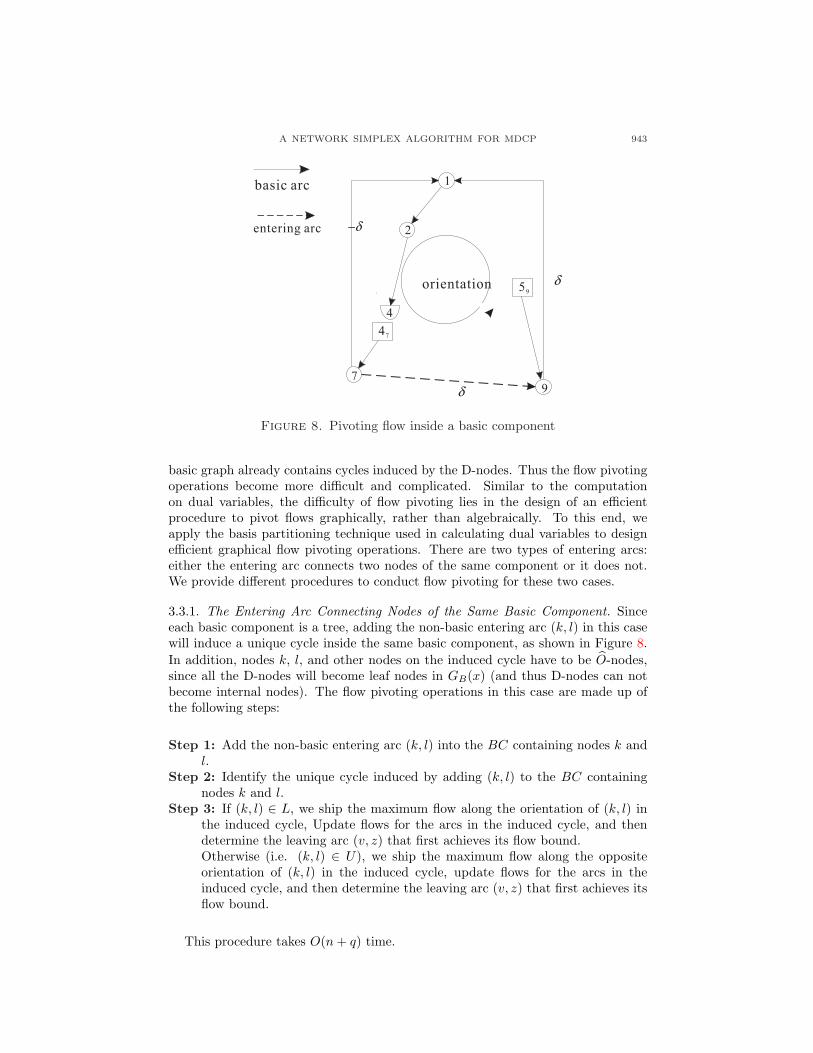
Figure 8. Pivoting flow inside a basic component

basic graph already contains cycles induced by the D-nodes. Thus the flow pivotingoperations become more difficult and complicated. Similar to the computationon dual variables, the difficulty of flow pivoting lies in the design of an efficientprocedure to pivot flows graphically, rather than algebraically. To this end, weapply the basis partitioning technique used in calculating dual variables to designefficient graphical flow pivoting operations. There are two types of entering arcs:either the entering arc connects two nodes of the same component or it does not.We provide different procedures to conduct flow pivoting for these two cases.

3.3.1. The Entering Arc Connecting Nodes of the Same Basic Component. Sinceeach basic component is a tree, adding the non-basic entering arc (k, l) in this casewill induce a unique cycle inside the same basic component, as shown in Figure 8.In addition, nodes k, l, and other nodes on the induced cycle have to be O-nodes,since all the D-nodes will become leaf nodes in GB(x) (and thus D-nodes can notbecome internal nodes). The flow pivoting operations in this case are made up ofthe following steps:

Step 1: Add the non-basic entering arc (k, l) into the BC containing nodes k andl.

Step 2: Identify the unique cycle induced by adding (k, l) to the BC containingnodes k and l.

Step 3: If (k, l) ∈ L, we ship the maximum flow along the orientation of (k, l) inthe induced cycle, Update flows for the arcs in the induced cycle, and thendetermine the leaving arc (v, z) that first achieves its flow bound.Otherwise (i.e. (k, l) ∈ U), we ship the maximum flow along the oppositeorientation of (k, l) in the induced cycle, update flows for the arcs in theinduced cycle, and then determine the leaving arc (v, z) that first achieves itsflow bound.

This procedure takes O(n + q) time.


3.3.2. The Entering Arc Connecting Nodes of Different Basic Components. Threetypes of end nodes for the entering arc (k, l) are possible in this case: (1) k ∈NO, l ∈ NO (2) k ∈ NO, l ∈ ND, and (3) k ∈ ND, l ∈ NO. In general, the enteringarc merges two components and reduces the number of basic components from p+1to p. Note that in this case the entering arc induces no cycle in the newly mergedcomponent, and thus we have to design a new graphical procedure to pivot flows.Here we will exploit the basis partitioning techniques used for calculating basic dualvariables in Section 3.2 to compute flows in the pivoting process.

To speed up the calculation, we conduct a graph compacting process to removethose nodes not eligible to ship flows in the pivoting graph, as well as their associatedarcs. In particular, two types of nodes are removable: (1) any O-node connectingwith one arc, and (2) any node inside a leaf basic component. This compactingprocedure may be repeated until all the O-nodes are connected with at least twobasic arcs and all the leaf basic components are removed. Since each compactingoperation removes at least one node and one basic arc, it takes a total of O(n + q)time.

The graph compacting procedure reduces the number of components in a pivotinggraph from p to p. G = (N , A) denotes the remaining pivoting graph after thecompacting process. We give four properties for G as follows:

Lemma 3.2. (i) Any leaf node in N is either a D-node or a side node.(ii) Any D-node i in N has to be adjacent to qi + 1 arcs.(iii) p ≤ min{p, n− p}.(iv) G contains p D-nodes.

Proof. (i) and (ii) are trivial since the compacting process removes all the leaf O-nodes, as well as those isolated D-nodes or side-nodes. We give the proof for (iii)and (iv) as follows:(iii) If p + 1 ≤ n− p, then we know that p < n− p and thus p ≤ p since the n− p

O-nodes can at most cover all the p components in the pivoting graph. On the otherhand, if p + 1 > n− p, then we know that p ≥ n− p and thus p ≤ n− p since then− p O-nodes can at most cover n− p of the p components in the pivoting graph.Therefore, p ≤ min{p, n− p}.(iv) The p components have to include the merged basic components induced bythe entering arc (k, l), since the entering arc is the source of any flow change. Thismeans that there were p + 1 basic components if we exclude the entering arc fromA. Since these p+1 basic components must be formed by detaching the distillationarcs from the p D-nodes, and these D-nodes will not be removed by (ii), so we knowN contains p D-nodes.

To conduct the flow pivoting operation, we have to identify the relationship offlow changes on basic arcs with respect to the flow change on the entering arc. Tothis end, we first set ∆kl = 1 (or ∆kl = −1) to represent the shipping of one unitof flow along the entering arc (k, l) if (k, l) ∈ L (or (k, l) ∈ U), and then for eachD-node i we assign the flow change along its incoming arc to be ∆i∗i (thus wehave in total p variables of ∆i∗i by Lemma 3.2(iii)). Using the flow distillation andbalance constraints, we can derive the flow change on each arc in A in terms of fi∗i

for each D-node i. Specifically, the flow in each distillation arc can be derived by


∆ij = kij∆i∗i for each D-node i. Since each component in G is a tree with leafnodes as D-nodes or side-nodes, all the flow change entering or leaving each leafnode can be expressed by ∆i∗i for each D-node i.

In addition, using the flow balance constraints associated with each internal node,we can conduct a search algorithm inside a component to traverse from leaf nodes toall other internal nodes and derive the flow change entering or leaving each internalnode in terms of ∆i∗i for each D-node i. Thus, for each component in G, we mayarbitrarily select an internal node as its root node and use the flow balance equationassociated with each root node to construct a system of p linear equations. Notethat this system of p linear equations has a rank equal to p − 1 since the flowbalance constraints have to be satisfied for each node and for the entire systemitself. Thus, one of the p flow balance equations can be removed. On the otherhand, by considering the additional equation ∆kl = 1 (or ∆kl = −1, depending onwhether (k, l) ∈ L or (k, l) ∈ U) representing the unit flow change for the enteringarc (k, l), a system of p linear equations can be constructed to solve the p variablesof ∆i∗i for each D-node i, and then all the relative flow changes on each arc in Acan be derived with respect to ∆kl.

Obtaining the relative flow change for each arc in A, we can conduct a minimumratio test to calculate θvz = min(i,j)∈A,∆ij 6=0{(uij − xij)/∆ij : ∆ij > 0,−xij/∆ij :∆ij < 0} for a leaving arc (v, z), update flows by xij = xij + θvz∆ij for each arc(i, j) in A with ∆ij 6= 0, and then remove (v, z) to form another basic graph for thenext iteration.

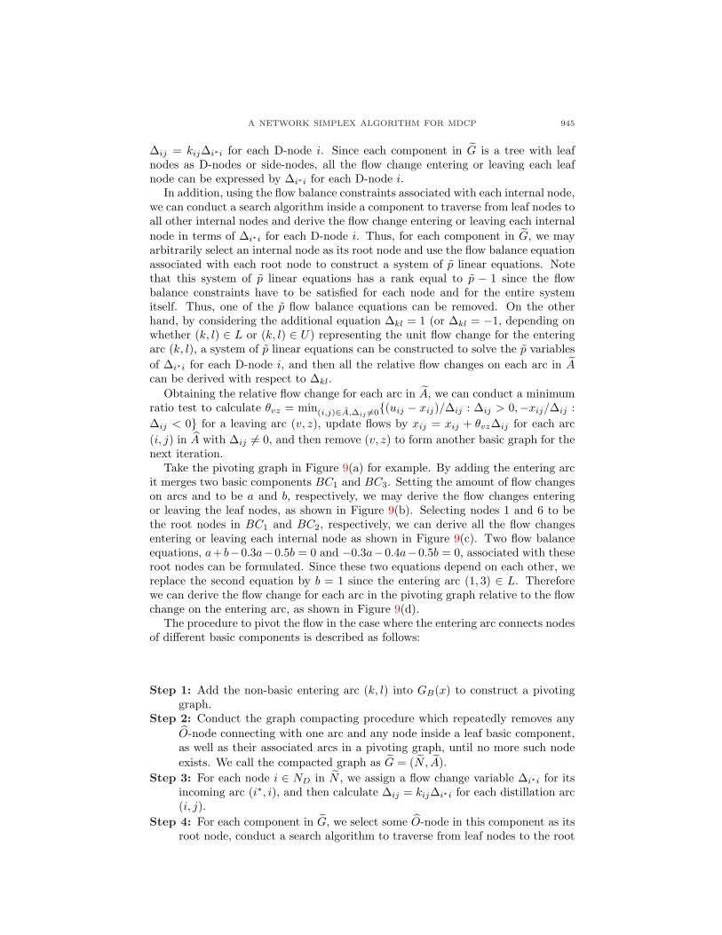
Take the pivoting graph in Figure 9(a) for example. By adding the entering arcit merges two basic components BC1 and BC3. Setting the amount of flow changeson arcs and to be a and b, respectively, we may derive the flow changes enteringor leaving the leaf nodes, as shown in Figure 9(b). Selecting nodes 1 and 6 to bethe root nodes in BC1 and BC2, respectively, we can derive all the flow changesentering or leaving each internal node as shown in Figure 9(c). Two flow balanceequations, a+ b−0.3a−0.5b = 0 and −0.3a−0.4a−0.5b = 0, associated with theseroot nodes can be formulated. Since these two equations depend on each other, wereplace the second equation by b = 1 since the entering arc (1, 3) ∈ L. Thereforewe can derive the flow change for each arc in the pivoting graph relative to the flowchange on the entering arc, as shown in Figure 9(d).

The procedure to pivot the flow in the case where the entering arc connects nodesof different basic components is described as follows:

Step 1: Add the non-basic entering arc (k, l) into GB(x) to construct a pivotinggraph.

Step 2: Conduct the graph compacting procedure which repeatedly removes anyO-node connecting with one arc and any node inside a leaf basic component,as well as their associated arcs in a pivoting graph, until no more such nodeexists. We call the compacted graph as G = (N , A).

Step 3: For each node i ∈ ND in N , we assign a flow change variable ∆i∗i for itsincoming arc (i∗, i), and then calculate ∆ij = kij∆i∗i for each distillation arc(i, j).

Step 4: For each component in G, we select some O-node in this component as itsroot node, conduct a search algorithm to traverse from leaf nodes to the root


( )a Add the entering arc (1,3) . ( )b Set variables to arc (2,4) and arc (3,5).

( )c Calculate all ( )d G

( )b=1

variables anda b

5

7

-

3

14

-

3

14

-

5

7

-

3

14

-3

14

2

7

-1

2

1

2

1

2

1

1

BC1

BC2

BC3

BC1

BC2

BC1

BC2

BC1

BC2

root

Figure 9. Computing the relative flow changes in a pivoting graph

node, and then derive the flow change on any arc inside that component usingthe flow balance constraints associated with each internal node.

Step 5: If (k, l) ∈ L, we solve the system of equations composed by ∆kl = 1 andthe flow balance constraints associated with p− 1 root nodes in N to obtain∆ij for each (i, j) ∈ A.Otherwise (i.e. (k, l) ∈ U), we solve the system of equations composed by∆kl = −1 and the flow balance constraints associated with p − 1 root nodesin N to obtain ∆ij for each (i, j) ∈ A.

Step 6: Calculate θvz = min(i,j)∈A,∆ij 6=0{(uij − xij)/∆ij : ∆ij > 0,−xij/∆ij :∆ij < 0} for a leaving arc (v, z).

Step 7: For each arc (i, j) ∈ A with ∆ij 6= 0, we update its flow by xij := xij +θvz∆ij .

The compacting procedure takes O(n + q − p) time to construct G. Setting theflow change variables for arcs connecting with D-nodes takes O(p + q) time, where


q represents the total number of distillation arcs in A. The search algorithm takesO(p(|A|− p− q)) time to derive the flow changes on the other arcs in A, since thereare |A| − p− q arcs in A with both end nodes to be O-nodes, and each flow changehas to be expressed using the p variables. Solving the system of p equations takesO(p3) time. The min-ratio test and flow updating operations for each arc in A takeO(|A|) time. Thus the procedure to calculate flow changes in the pivoting graphcan be done in O(p3 + p|A| + n + q) ≤ O(min{p3 + np, (n − p)3 + n(n − p)} + q)time, since p ≤ min{p, n− p} by Lemma 3.2(iii).

Different from our basis partitioning technique, Sheu et al. [19] proposed adifferent partitioning technique to calculate the flow change on each arc in a givenaugmenting subgraph for solving a maximum flow problem in a distribution network.After constructing the compacted pivoting graph G = (N , A), we can use p O-nodesconnected with more than two arcs as the dividing nodes to divide G into p + 1compatible components, where the flow change on each arc inside a component can beexpressed by a single variable. After solving the system of p+1 equations composedby the flow balance equations associated with p dividing nodes and ∆kl = 1 (or∆kl = −1, depending on whether (k, l) ∈ L or (k, l) ∈ U ), the flow change on eacharc in A can be expressed by ∆kl. Since there are at most p such O-nodes andp = O(n − p), their technique takes O((n − p)3) time. Therefore, our technique isat least asymptotically similar to theirs for the cases with more D-nodes. For thecases with fewer D-nodes than O-nodes, our technique is asymptotically faster thantheirs.

3.4. Updating dual variables. After pivoting the flows and removing the leavingarc, the network simplex algorithm updates dual variables for the new basic graph.The new dual variables associated with the updated basic graph can be calculatedfrom scratch using the procedure proposed in Section 3.2. However, since the basicgraphs of two successive pivoting iterations share many common components, amore efficient dual variable update scheme can take advantage of the basic graph ofthe previous iteration. In this paper we propose a dual variables update procedurethat exploits the structure of the basic components in the previous procedure andsaves more computational efforts than the procedure in Section 3.2.

Let bc(i) and bc(ij) represent the index of the basic component containing thenode i ∈ N and the side-node ij , respectively. Suppose GB(x) is a basic graphin some network simplex iteration before flow pivoting, and that the flow pivotingprocedure selects (k, l) and (v, z) to be the entering and leaving arc, respectively.Let g = bc(k), h = bc(l), and w = bc(z). If we remove the leaving basic arc (v, z)from GB(x), BCw will be split into two basic components: BCbc(z) and BCbc(v).For the sake of convenience, let bc(z) = w and bc(v) = p + 2, and there are atotal of p + 2 basic components in the pivoting graph, excluding the entering andleaving arcs. Since all the arcs in these p + 2 basic components remain basic, dualvariables still satisfy equations (20) and (21). Thus, dual variables inside each ofthese p + 2 basic components will have the same amount of change, but differentbasic component may have a different amount of change. Let δα record the changefor each dual variable inside BCα for α = 1, ..., p + 2. Let πold

i , ρoldij and πnew

i ,ρnew

ij denote dual variables associated with a node i ∈ N and a distillation arc(i, j) ∈ A in two successive network simplex iterations, respectively. Then, πnew

i :=πold

i + δbc(i)and ρnewij := ρold

ij + δbc(ij).


Adding the non-basic entering arc (k, l) to the p+2 basic components merges BCg

and BCh into a new and larger component BCg ∪BCh in the pivoting graph. Forthe sake of convenience, let BCg := BCg ∪ BChand BCh := BCp+2. This mergerintegrates the variables of two components and reduces the number of componentsand variables by one. Now we only need to consider p + 1 components (i.e. BCα

for α = 1, 2, ..., p + 1). Depending on the type of node k, δh can be expressed by δg

using one of the following two equations:

1. If node k is an O-node, it satisfies:

πnewk − πnew

l = ckl

=⇒πoldk + δg − πold

l − δh = ckl

=⇒δh = δg − ckl − πoldl + πold

k (26)

2. If node k is a D-node, it satisfies:

ρnewkl − πnew

l = ckl

=⇒ ρoldkl + δg − πold

l − δh = ckl

=⇒ δh = δg − ckl − πoldl + ρold

kl (27)

Now we can form a system of p + 1 equations composed by δg = 0, as wellas the p equations of δbc(i) =

∑j∈L(i) kijδbc(ij) for each D-node i. Moreover, each

equation can be expressed using p+1 variables composed δα by for α = 1, 2, ..., p+1.Therefore, the amount of change for each dual variable can be calculated by solvingthis system of p + 1 linear equations.

Similar to the procedure in Section 3.2, we may speed up the procedure byupdating dual variables for those non-leaf basic components first, and then later forthe leaf basic components. The procedure to update dual variables is as follows:

Step 0: Initialize H := ∅, ND1 := ∅, where H stores the indices of leaf basiccomponents, and ND1 stores the indices of the D-node associated with leafbasic components.Let πold

i and ρoldij denote the original dual variable associated with a node

i ∈ N and a distillation arc (i, j) ∈ A, respectively.For each node i and side-node ij , set bc(i) and bc(ij) to be the index of thebasic component that contains i and ij , respectively.

Step 1: Remove the leaving arc (v, z) and split BCbc(z) into BCbc(z) and BCbc(v).For the sake of convenience, let w := bc(z) and bc(v) := p + 2.For each basic component α = 1, ..., p + 2, let δα represent the amount ofchange for each dual variable inside BCα.For the entering arc (k, l), let g := bc(k) and h := bc(l).

Step 2: Calculate δh by δg using δh = δg − πoldl + πold

k − ckl or δh = δg − πoldl +

ρoldkl − ckl, depending on whether node k is an O-node or a D-node.

Step 3: Add the entering arc (k, l) to merge BCh into BCg. For the sake ofconvenience, let BCg := BCg ∪BCh and BCh := BCp+2.

Step 4: Identify the leaf basic components, add their indices into H, and add theirassociated D-nodes into ND1.

Step 5: Set δr = 0 for some BCr not in H.Step 6: Solve the system of equations composed by δbc(i) =

∑j∈L(i) kijδbc(ij) :

∀i ∈ ND\ND1 and δr = 0.


Step 7: Solve the remaining δk : k ∈ H by δbc(i) =∑

j∈L(i) kijδbc(ij) : ∀i ∈ ND1.Step 8: Update each dual variable by πnew

i = πoldi +δα or ρnew

jk = ρoldjk + δαfor each

node i and side-node jk.

Although this procedure is practically faster than the procedure in Section 3.2,it has the same theoretical complexity as O(min{p3, (n− p)3}+ n + p).

4. Conclusions. To efficiently solve the minimum distribution cost problem pro-posed by Fang and Qi [8], this paper provided the first detailed graphical proceduresto implement the network simplex algorithm. We have carefully designed a basisportioning technique to decompose a basic graph into several basic componentsdivided by D-nodes, where each component corresponds to a tree. We also pro-vided sound theoretical background to support our algorithm, and proposed a setof graphical operations to efficiently conduct the calculation for both primal anddual variables. With our techniques, many computational efforts for calculatingthe basic variables can be reduced, compared to other methods in the literature.Techniques to speed up our algorithm have also been investigated with theoreticalsupport. Although omitted in this paper, for future research, we suggest investigat-ing the degeneracy issues, which are usually encountered in simplex-like algorithms.

Acknowledgments. We would like to thank referee and editor for their valuablecomments. I-Lin Wang was partially supported by the National Science Council ofTaiwan under Grant NSC95-2221-E-006-268.

REFERENCES

[1] R. K. Ahuja, T. L. Magnanti and J. B. Orlin, “Network Flows: Theory, Algorithms andApplications,” Prentice Hall, Englewood Cliffs, New Jersey, U.S.A., 1993.

[2] R. Barr, F. Glover and D. Klingman, Enhancements to spanning tree labeling procedures fornetwork optimization, INFOR, 17 (1979), 16–34.

[3] G. H. Bradley, G. G. Brown and G. W. Graves, Design and implementation of large scaleprimal transshipment algorithms, Management Science, 24 (1977), 1–34.

[4] M. D. Chang, C. H. J. Chen and M. Engquist, An improved primal simplex variant for pureprocessing networks, ACM Transactions on Mathematical Software, 15 (1989), 64–78.

[5] C. H. J. Chen and M. Engquist, A primal simplex approach to pure processing networks,Management Science, 32 (1986), 1582–1598.

[6] E. Cohen and N. Megiddo, Algorithms and complexity analysis for some flow problems, Al-gorithmica, 11 (1994), 320–340.

[7] E. W. Dijkstra, A note on two problems in connexion with graphs, Numerische Mathematik,1 (1959), 269–271.

[8] S. C. Fang and L. Qi, Manufacturing network flows: A generalized network flow model formanufacturing process modeling, Optimization Methods and Software, 18 (2003), 143–165.

[9] L. R. Ford and D. R. Fulkerson, Maximal flow through a network, Canadian Journal ofMathematics, 8 (1956), 399–404.

[10] F. Glover, D. Karney and D. Klingman, Implementation and computational comparisonsof primal, dual and primal-dual computer codes for minimum cost network flow problems,Networks, 4 (1974), 191–212.

[11] F. Glover, D. Karney, D. Klingman and A. Napier, A computation study on start procedures,basis change criteria and solution algorithms for transportation problems, Management Sci-ence, 20 (1974), 793–813.

[12] F. Glover, D. Klingman and J. Stutz, Augmented threaded index method for network opti-mization, INFOR, 12 (1974), 293–298.

[13] E. L. Johnson, Networks and basic solutions, Operations Research, 14 (1966), 619–623.[14] J. L. Kennington and R. V. Helgason, “Algorithms for Network Programming,” John Wiley

& Sons, New York, NY, USA, 1980.


[15] J. L. Kennington and R. V. Helgason, Minimum cost network flow algorithms, In “M.G.C.Resende and P.M. Pardalos, editors, Handbook of Optimization in Telecommunications,”chapter 6, 147–162. Springer, 2006.

[16] J. Koene, “Minimal Cost Flow in Processing Networks, A Primal Approach,” PhD thesis,Eindhoven University of Technology, Eindhoven, The Netherlands, 1982.

[17] H. Lu, E. Yao and L. Qi, Some further results on minimum distribution cost flow problems,Journal of Combinatorial Optimization, 11 (2006), 351–371.

[18] J. Mo, L. Qi and Z. Wei, A network simplex algorithm for simple manufacturing networkmodel, Journal of Industrial and Management Optimization, 1 (2005), 251–273.

[19] R. L. Sheu, M. J. Ting and I. L. Wang, Maximum flow problem in the distribution network,Journal of Industrial and Management Optimization, 2 (2006), 237–254.

[20] P. Venkateshan, K. Mathur and R. H. Ballou, An efficient generalized network-simplex-based algorithm for manufacturing network flows, Journal of Combinatorial Optimization,15 (2008), 315–341.

[21] I. L. Wang and J. C. Lin, Solving maximum flows on distribution networks: Network com-paction and algorithm, In “Proceedings of the 10th Annual Conference of the Asia-PacificDecision Science Institute (APDSI),” Taipei, Taiwan, June 2005.

[22] I. L. Wang and Y. H. Yang, On solving the uncapacitated minimum cost flow problems in adistribution network, International Journal of Reliability and Quality Performance, 1 (2008),53–63.

Received October 2008; 1st revision June 2009; final revision July 2009.E-mail address: [email protected]

E-mail address: [email protected]

a network simplex algorithm for solving the … · a network simplex algorithm for solving the...

Documents