WATER AND ENERGY SECTOR VULNERABILITY TO CLIMATE WARMING IN THE SIERRA NEVADA: Simulating the Regulated Rivers of California’s West Slope Sierra Nevada 

 

 A White Paper from the California Energy Commission’s California Climate Change Center 

JULY  2012

CEC ‐500 ‐2012 ‐016  

Prepared for:  California Energy Commission 

Prepared by:  University of California, Davis  

David E. Rheinheimer Scott T. Ligare Joshua H. Viers  University of California, Davis Davis, California, 95616 USA  

DISCLAIMER

This paper was prepared as the result of work sponsored by the California Energy Commission. It does not necessarily represent the views of the Energy Commission, its employees or the State of California. The Energy Commission, the State of California, its employees, contractors and subcontractors make no warrant, express or implied, and assume no legal liability for the information in this paper; nor does any party represent that the uses of this information will not infringe upon privately owned rights. This paper has not been approved or disapproved by the California Energy Commission nor has the California Energy Commission passed upon the accuracy or adequacy of the information in this paper.

i

ACKNOWLEDGEMENTS

This research was made possible by funding from the California Energy Commission. We would like to thank Mike Kiparsky (University of Idaho) for providing computational support, as well as Jack Sieber, Vishal Mehta, and other staff at the Stockholm Environment Institute for providing and supporting WEAP21. We also thank past and present students Shannon Brown, Erik Moreno, and Danielle Salt for their modeling assistance. Finally, we thank the anonymous reviewers of this work for their valuable comments.

ii

ABSTRACT

Climate warming is expected to affect the beneficial uses of water in the Sierra Nevada, impacting nearly every resident of California. This paper describes the development and results from an integrated water resource management model encompassing water operations and hydropower generation for the west slope Sierra Nevada spanning the Feather River basin in the north to the Kern River basin in the south at the weekly time step. This model application includes management of reservoirs, run-of-river hydropower plants, water supply demand locations, conveyances, and instream flow requirement. Model validation indicates that most major hydropower turbine flows were simulated well, with wetter years modeled more effectively than drier years. The results of this work indicated that hydropower generation will be reduced by approximately 8 percent with 6°C (10.8°F) warming, consistent with other studies, with a conservative parameterization of no change in precipitation. Reservoir operations adapt to capture earlier and greater runoff volumes that result from earlier and greater runoff due to climate warming. Seasonal compensation in operations is insufficient to overcome warming mediated losses.

Keywords: water energy nexus, water management, climate change, non-stationary climate, regulated rivers, reservoirs, habitat, Sierra Nevada

Please use the following citation for this paper:

Rheinheimer, D. R., S. T. Ligare, and J. H. Viers (Center for Watershed Sciences, University of California, Davis). 2012. Water-Energy Sector Vulnerability to Climate Warming in the Sierra Nevada: Simulating the Regulated Rivers of California’s West Slope Sierra Nevada. California Energy Commission. Publication number: CEC-500-2012-016.

iii

TABLE OF CONTENTS

Acknowledgements ................................................................................................................................... i 

ABSTRACT ............................................................................................................................................... ii 

TABLE OF CONTENTS ......................................................................................................................... iii 

LIST OF FIGURES .................................................................................................................................. iv 

LIST OF TABLES ...................................................................................................................................... v 

Section 1: Summary .................................................................................................................................. 1 

Section 2: Introduction ............................................................................................................................. 2 

Section 3: Background .............................................................................................................................. 3 

3.1. Water Resources in the Sierra Nevada ......................................................................................... 3 

3.2 Regional Climate Warming ............................................................................................................ 3 

3.3 Regional Water Resources Management Models ........................................................................ 3 

Section 4: Methods .................................................................................................................................... 6 

4.1 Model Scope ...................................................................................................................................... 6 

4.2 Infrastructure .................................................................................................................................... 6 

4.3 Water Evaluation and Planning System (WEAP) ........................................................................ 8 

4.4 Inflow Hydrology ............................................................................................................................ 9 

4.5 Universal Parameters .................................................................................................................... 10 

4.6 Reservoirs ........................................................................................................................................ 11 

Storage Capacity ............................................................................................................................... 11 

Initial Storage .................................................................................................................................... 11 

Volume-Elevation Curves ............................................................................................................... 11 

Reservoir Zone Operations ............................................................................................................. 11 

Lake Evaporation ............................................................................................................................. 12 

4.7 Hydropower ................................................................................................................................... 12 

Water Year Index Method ............................................................................................................... 12 

Spill Demand Method ..................................................................................................................... 16 

4.8 Water Supply Demand .................................................................................................................. 17 

4.9 Instream Flow Requirements ....................................................................................................... 17 

4.10 Diversions ..................................................................................................................................... 18 

iv

4.11 Priority Setting .............................................................................................................................. 18 

4.12 Interbasin Transfers ..................................................................................................................... 19 

4.13 Integrating Models and Data Management ............................................................................. 19 

4.14 Climate Change Scenarios .......................................................................................................... 20 

Section 5: Calibration and Model Assessment .................................................................................. 21 

5.1 Hydropower Turbine Flow .......................................................................................................... 22 

5.2 Reservoir Storage and Evaporation ............................................................................................. 26 

Section 6: Results with Warming ......................................................................................................... 28 

6.1 WEAP Runoff Scenarios: Air Temperature Increase ................................................................ 28 

6.2 VIC Runoff Scenarios: Downscaled GCM Output .................................................................... 34 

Section 7: Limitations ............................................................................................................................. 38 

Section 8: Conclusions ........................................................................................................................... 40 

References................................................................................................................................................. 41 

Appendix A: SIERRA Input Parameters ........................................................................................... 45 

LIST OF FIGURES

Figure 1: Included Features in the Regulated Sierra Nevada Model .................................................. 7 

Figure 2: WEAP Model Process ............................................................................................................... 9 

Figure 3: Historical San Joaquin Valley Water Year Index (WYI) and Big Creek No. 1 powerhouse turbine flow for the weeks of July 25–31 and November 7–13 ................................... 15 

Figure 4: Seasonal NSME by Mean Modeled Turbine Flow .............................................................. 23 

Figure 5: Observed and Modeled Mean Annual and Seasonal Hydropower Turbine Flow ........ 24 

Figure 6: Observed and Simulated Mean Annual and Seasonal Hydropower Generation .......... 25 

Figure 7: Total Observed and Modeled Hydropower Generation ................................................... 25 

Figure 8: Observed and Modeled Mean Annual and Seasonal Reservoir Storage ......................... 26 

Figure 9: Mean (WY1981–2000) Mean Lake Evaporation for Lake Almanor Using Observed (CDEC) and Modeled Storage Data ...................................................................................................... 27 

Figure 10: Mean Total Weekly Energy Generation with Warming .................................................. 29 

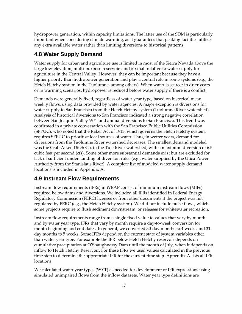
Figure 11: Seasonal and Annual Hydropower Generation with Warming ..................................... 30 

v

Figure 12: Seasonal Hydropower Generation Change by Watershed .............................................. 31 

Figure 13: Mean Annual Hydropower Generation Change by Watershed ..................................... 32 

Figure 14: Total Sierra Nevada Storage for Modeled Reservoirs with Warming ........................... 34 

Figure 15: Mean Annual Hydropower Generation by Hydrologic and climate Model with Warming .................................................................................................................................................... 36 

LIST OF TABLES

Table 1: Count of Modeled Features in SIERRA (ordered north to south) ........................................ 8 

Table 2: Modeled Features and Attributes ............................................................................................. 9 

Table 3: Priority Assignments for Two Hypothetical Projects........................................................... 19 

Table 5: Model Performance Metrics for Fixed Head Hydropower Turbine Flow ........................ 23 

Table 6: Seasonal and Annual Hydropower Generation Change with Warming .......................... 29 

Table 7: Mean Annual Hydropower Generation Change with +6°C Warming by Watershed .... 32 

Table 8: Mean Annual Hydropower Generation (GWh) by GCM and Time Span with Percent Change from Historical Climate Conditions ........................................................................................ 35 

Table 9: Mean Annual Hydropower Generation by Basin and Time Span with Mean, Range, and Percent Change from Historical Climate Conditions ......................................................................... 37 

Unless otherwise noted, all tables and figures are provided by the author.

1

Section 1: Summary

In California’s Sierra Nevada Mountains, water is managed for hydropower production, instream flows, urban and agricultural water supply, recreation, and flood regulation, affecting nearly every resident of California. However, there is currently no single model or tool that can be used to assess multi-sector effects of changes in physical and other conditions that will be affected by climate warming, such as inflow hydrology. Climate warming is expected to alter runoff magnitude and timing in the Sierra Nevada, affecting all beneficial uses of water. Spring/summer snowmelt runoff will decrease, while winter runoff from precipitation will increase, shifting runoff timing to earlier in the year. Warming will also decrease total runoff. , Existing studies quantifying effects of climate warming on water resources in the Sierra Nevada are either temporally coarse (monthly), limited in spatial extent (single watersheds), or single-purpose. In this study, we sought to improve understanding of how regulated flows in the Sierra Nevada may be vulnerable to climate warming and to help develop adaptation strategies to manage water resources for competing demands. To do this, we developed a weekly time step water resources management model for the west slope Sierra Nevada, from the Feather River watershed in the north to the Kern River watershed in the south. The model is developed with the Water Evaluation and Planning (WEAP) modeling system and includes management of reservoirs, run-of-river hydropower plants, water supply demand locations, conveyances, and instream flow requirements. The model is applied with two different datasets to represent runoff with historical-, near-, mid-, and far-term warming: one that uses WEAP and considers regional air temperature increases of 0°C, 2°C, 4°C, and 6°C (0°F, 3.6°F, 7.2°F, and 10.8°F) and another that uses the variable infiltration capacity (VIC) hydrologic model with downscaled global circulation model (GCM) climate data.

Key findings include:

Most major hydropower turbine flows are simulated well. Reservoir storage is also generally well simulated, mostly limited by the accuracy of inflow hydrology.

With air temperature increase of 6°C, system wide hydropower generation is reduced by 9 percent.

Most reductions in hydropower generation occur in the highly productive watersheds in the northern Sierra Nevada. The central Sierra Nevada sees less reduction in annual runoff and can adapt better to changes in runoff timing. Generation in southern watersheds is expected to decrease.

Reservoirs adapt to capture earlier runoff, but mostly decrease in mean reservoir storage with warming due to decreasing annual runoff.

We highlight important model limitations and recommend improvements, including refining representation of climate change effects and a more sophisticated, project-specific hydropower simulation method.

2

Section 2: Introduction

Climate warming is expected to affect the beneficial uses of water in California’s Sierra Nevada Mountains, including hydropower, water supply, ecosystem benefits, and flood control, directly affecting nearly every resident of California. However, no single model or tool is available to assess potential regional vulnerabilities to climate change across a range of water use sectors in sufficient detail to inform management decisions.

To help fill this management information gap, we developed a watershed scale, weekly time step simulation model of regulated flows for 15 watersheds in the upper Sierra Nevada, called the Sierra Integrated Environmental and Regulated Rivers Assessment (SIERRA) model. This paper describes the model scope, methods, calibration, a subset of results, and a summary of model limitations and recommendations for improvement. Results from a model as comprehensive in management scope as SIERRA are extensive. This study focuses on hydropower generation, the dominant management objective in the upper Sierra Nevada. Focusing on hydropower also allows for comparisons of results with other regional models.

SIERRA builds directly on the work of Young et al. (2009) and Mehta et al. (2011). Young et al. (2009) used the Water Evaluation and Planning system (WEAP) to model the unimpaired hydrology of 15 major watersheds in the western Sierra Nevada. SIERRA spans the same geographic region, uses the same set of climate change scenarios (+0°C, 2°C, 4°C, and 6°C warming), and the same temporal resolution (weekly time steps) as the WEAP-based hydrologic model. Mehta et al. (2011) developed a water management simulation model using WEAP to study the effects of climate change on hydropower in the Cosumnes, American, Bear and Yuba River watersheds using the runoff results of Young et al. (2009). SIERRA modifies the work of Mehta et al. (2011) with improved simulation methods.

This study is an outcome-based vulnerability assessment. In an outcome-based vulnerability assessment, vulnerability is defined as the effect of climate change on the managed domain of interest (e.g., hydropower generation), as mediated by exposure, sensitivity to changes in exposure, and system adaptive capacity (California Natural Resources Agency 2009; O'Brien et al. 2007). In this study, which is a study of water management, the specific exposure units—variables that are directly sensitive to climate variables such as air temperature and precipitation—include runoff, evaporation from reservoirs, and operations decisions that depend directly on precipitation or runoff.

Sensitivity of hydropower generation to climate changes is measured by system behavior at discrete levels of regional climate change. The study was conducted primarily using a hydrologic model results that approximates future climate conditions with uniform increases in air temperature. In addition, sensitivity to changes using a hydrologic model applied with downscaled climate data from general circulation model (GCMs) is considered. The details of these climate exposures are discussed in further detail. System adaptive capacity is not quantified explicitly, though many infrastructure operating rules in the model are inherently adaptive. For example, methods used to minimize spill from reservoirs enable some adaptation to warming-induced changes in runoff timing.

3

Section 3: Background

3.1. Water Resources in the Sierra Nevada

Water infrastructure in the upper Sierra Nevada, at elevations above about 300 m (1000 ft), is managed primarily for hydropower. Some high-elevation infrastructure is also managed explicitly for local and regional water supply, recreation, and flood regulation. High elevation water systems also have implicit water supply and flood regulation roles at the watershed scale by providing inflows to the major water projects of the Central Valley and by providing incidental flood storage space at the watershed scale(e.g., Hickey et al. 2003).

In California, hydropower generation supplies about 15 percent of the total electricity production. Hydropower systems in the Sierra Nevada provide roughly 75 percent of California’s in-state hydropower, approximately 20,000 GWh annually, primarily from more than 150 reservoirs higher than 350 m above sea level (Aspen Environmental Group and M Cubed 2005).

3.2 Regional Climate Warming

Global climate warming will alter hydrology on global, regional, and local scales (Bates et al. 2008). Climate warming is expected to reduce snowpack, decrease mean annual flow, and lead to earlier spring snowmelt runoff in the western United States, including the Sierra Nevada (Dettinger et al. 2004; Hayhoe et al. 2004; Tanaka et al. 2006; Vicuna et al. 2007).

Hydrologic changes will affect hydropower production, urban and agricultural supply, recreation and other beneficial uses such as aquatic and terrestrial ecosystems (Hayhoe et al. 2004; Madani and Lund 2010; Medellín-Azuara et al. 2008; Null et al. 2010; Tanaka et al. 2006). While it is widely understood that warming will affect hydrology-dependent systems in the Sierra Nevada, few models quantify specific effects. These models are discussed below.

3.3 Regional Water Resources Management Models

Several water resources management models exist that include some aspect of watershed-scale water resources in the upper Sierra Nevada. All models of upper Sierra Nevada water systems are single-purpose (i.e., flood control, hydropower, and water resources. Existing models that include most of the upper Sierra Nevada are temporally coarse, generally monthly-scale, and also single-purpose. Some local models have greater temporal resolution (e.g., Vicuna et al. 2008). Models of California’s major water supply systems such as CALVIN (Medellín-Azuara et al. 2008; Tanaka et al. 2006) and CalSim II (Draper and Darabzand 2003) exclude most high-elevation water systems above the large, low-elevation, multi-purpose reservoirs, yet rely on runoff from the Sierra Nevada as boundary inflows.

Two single-purpose reservoir management models have been developed that span most of the western Sierra Nevada. Hickey et al. (2003) included 73 flood reduction reservoirs, including 40 high-elevation Sierra Nevada reservoirs, in a HEC-5(U.S. Army Corps of Engineers (USACE) 1998) synthetic flood hydrograph simulation model for California’s Central Valley. Madani and Lund (2009) modeled monthly hydropower generation in

4

California for elevations higher than 300 m (1000 ft), including most hydropower reservoirs in the Sierra Nevada, by describing reservoir storage in energy units and using the Energy-Based Hydropower Optimization Method (EBHOM) and assuming no annual spill. As these models are tailored to addressing specific water use purposes, they do not enable estimating regulated flows in specific locations.

Numerous models have been developed for operations planning for individual watersheds or systems in the western Sierra Nevada for flood control, hydropower, and water supply. For instance, the Pacific Gas & Electric Company (PG&E) uses an optimization model that incorporates probabilistic inflows to help plan operations of its hydropower systems (Jacobs et al. 1995), which span a substantial portion of the western Sierra Nevada.

Several models have been developed to study potential impacts of climate change on hydropower systems with local case studies (Mehta et al. 2011; Vicuna et al. 2009; Vicuna et al. 2008) and to study broad impacts across the Sierra Nevada at the monthly scale (Madani and Lund 2010). Using a range of downscaled climate conditions from two emissions and six general circulation model (GCM) scenarios, Vicuna et al. (2009) estimated decreases in energy production of 12.2 percent in the Upper American River Project (UARP) system and 10.4 percent in the Big Creek System (San Joaquin River watershed) by end-of-century, when averaged across emissions and GCM scenarios. These results are from corresponding decreases in mean annual runoff of 10.1 percent in the UARP system and 17.8 percent in the Big Creek System.

Mehta et al. (2011) developed a weekly scale model of the Cosumnes, American, Bear, and Yuba (CABY) watersheds in the western Sierra Nevada using the Water Evaluation and Planning system (WEAP) (Yates et al. 2005) to simulate changes in water management with regional climate warming. Assuming uniform air temperature increase of 0°C, 2°C, 4°C, and 6°C, as described by Young et al. (2009), they estimated a decrease in hydropower generation of almost 20 percent in the Yuba-Bear/Drum-Spaulding project in the upper Yuba River and Bear River watersheds and of 22 percent in the Middle Fork Project in the American River watershed. The model described here builds on the work of Mehta et al. (2011).

At the state-wide scale, Madani and Lund (2010) applied EBHOM (Madani and Lund 2009) to estimate effects of warming, with wet, dry, and warming-only conditions, on high-elevation hydropower generation. With warming-only—i.e., a change in runoff timing to earlier in the year, but with no change in total annual runoff—Madani and Lund (2010) estimated a decrease in energy generation California-wide by a much more modest 1.3 percent using hydrology from 1985–1988. With drier conditions (less runoff), they estimated decreases of almost 20 percent.

These studies demonstrate that annual generation is much more positively dependent on total annual runoff than on changes in runoff timing and that by end-of-century, hydropower production will likely decrease substantially due to decreased average annual runoff. This is due to the ability of hydropower systems to adapt, at least partially, to changes in runoff timing. Most regional climate change adaptation models inherently adapt to changes in timing because they use optimization methods; it is therefore essential to incorporate system adaptive capacity in a rule-based simulation model.

5

These anticipated impacts on hydropower generally mean that changing climate conditions need to be considered in long term, regional planning of water resources in the Sierra Nevada, as water users will be under ever greater pressure to maintain services and revenues by continuing to operate in ways that potentially harm other water users, including the environment.

Previous studies are collectively limited in geographic scope, management domain, and/or temporal scope. The goal of this work was to fill some of these gaps by including most of the water management infrastructure in the western Sierra Nevada in multi-reservoir simulation model framework and by using a finer temporal resolution.

6

Section 4: Methods

The primary objective of this work was to create a model that simulates the operations of all major upper Sierra Nevada water management in a way that is sensitive to climate changes and that can be readily improved for future studies. The model scope and the physical characteristics and operational logic of modeled features are described.

4.1 Model Scope

The modeling goal was to simulate dominant operations of major water management infrastructure in the upper west slope of the Sierra Nevada, including reservoirs, hydropower, water supply, and environmental flows, with air temperature a primary variable for operations. Modeled watersheds include, from north to south, the Feather (FEA), Yuba/Bear (YUB), American/Cosumnes (AMR), Mokelumne (MOK), Calaveras (CAL), Stanislaus (STN), Tuolumne (TUO), Merced (MER), San Joaquin (SJN), Kings (KNG), Kaweah (KAW), Tule (TUL), and Kern (KRN) River watersheds (Figure 1). The American, Bear and Yuba (ABY) Rivers are modeled and analyzed together due to their low-elevation inter-basin transfers; there is no hydropower in the Cosumnes (part of “CABY”). Most major infrastructure above the large, low-elevation dams are included, as described below. The Cosumnes, Calaveras and Merced watersheds lack major regulating infrastructure above their terminal dams; these watersheds are modeled, but excluded from analyses.

SIERRA was developed and applied using weekly time steps. For this study, SIERRA uses inflow data from Water Year (WY) 1981–2000, as developed by Young et al. (2009) for baseline operations. This time span is useful because it includes a wide range of recent historical climatic and discharge conditions typical of the region, including an extended drought (1987–1992), the wettest year on record (1983), and the flood year of record (1997).

4.2 Infrastructure

SIERRA includes (Table 1) reservoirs, fixed head hydropower, variable head hydropower, supply demands, instream flow requirements, and conveyances. This includes most major infrastructure elements in each watershed above the large, low-elevation, multi-purpose "rim" dams, exclusive of most rim dams. Most rim reservoirs were excluded, due to the added complexity of modeling flood regulation and water deliveries to the Central Valley. Exceptions include Lake Isabella (KRN), New Bullards Bar Dam (YUB), and Camp Far West Reservoir (YUB). All reservoirs listed by the California Data Exchange Center (CDEC) and within the study area were included. Most small reservoirs such as diversion reservoirs and forebays are excluded, with some exceptions. A complete list of modeled infrastructure and their characteristics is included in Appendix A.

Most hydropower projects are fixed head powerhouses, including both high head powerhouses typical of the Sierra Nevada and run-of-river powerhouses below small reservoirs. There are also a few conventional, variable head powerhouses. Small, private hydropower plants were generally omitted, with the exception of Kanaka Power plant (Feather River watershed). The distinction between fixed head and variable head is important in WEAP.

7

Water supply demands were included where data were available or where a diversion for water supply clearly exists. Diversions in the Sierra Nevada for water supply are small relative to water supply (mostly irrigation) for the Central Valley. A few small water supply diversions are not parameterized pending further development.

Figure 1: Included Features in the Regulated Sierra Nevada Model

8

Table 1: Count of Modeled Features in SIERRA (ordered north to south)

Model code Watershed

Fix

ed h

ead

h

ydro

Var

iabl

e h

ead

h

ydro

Res

ervo

irs

Su

pp

ly

dem

ands

Inst

ream

flo

w

req

’t

Con

veya

nce

Tot

al

FEA Feather River 16 2 10 3 18 20 69

ABY Yuba River / Bear River

17 5 12 11 20 23 88

American River 9 5 12 3 15 17 61

Cosumnes River 1 1 1 3

MOK Mokelumne River 4 1 2 2 7 9 25

CAL Calaveras River 0

STN Stanislaus River 8 2 6 11 12 49

TUO Tuolumne River 3 3 1 3 6 16

MER Merced River 0

SJN San Joaquin River 15 1 8 19 21 64

KNG Kings River 4 2 5 5 16

KAW Kaweah River 3 4 5 12

TUL Tule River 2 5 1 2 10

KRN Kern River 5 1 5 5 16

86 16 58 25 109 126 419

4.3 Water Evaluation and Planning System (WEAP)

SIERRA uses the Water Evaluation and Planning System (WEAP21 or WEAP) software. WEAP is a water resources modeling platform that integrates a two-soil layer, one-dimensional hydrologic model with a priority-based water resources management model (Yates et al. 2005). SIERRA uses WEAP’s water management module, with runoff (inflow) represented as exogenous variables.

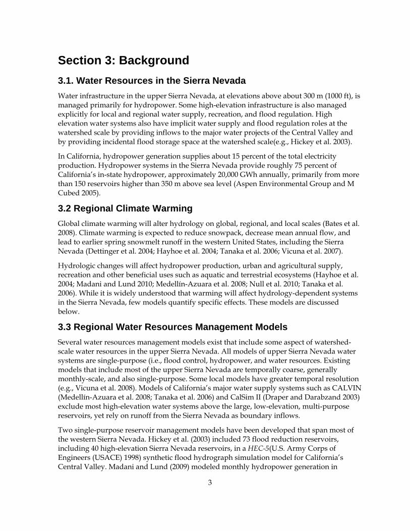
To simulate operations accurately, WEAP requires features and their physical parameters and operating rules, initial conditions, and boundary conditions (Figure 2). Operating rules represent the infrastructure management decisions for when and where to release water. In WEAP, these are provided as expressions, which vary from a single integer value to a call to an external script. Expressions can include mathematical operators, logical functions, and a range of built-in modeling functions. SIERRA relies on expressions to define input data and link to external lookup tables and scripts. Major inputs to the regulated model, including classes of modeled features and feature attributes, are listed in Table 2, with methods described below.

Climate change effects can be represented in SIERRA by changing boundary conditions, including meteorological conditions, which affect reservoir evaporation, and inflow time series. Climate change can also indirectly affect management in SIERRA through operating rules that depend on inflow and meteorology.

9

Figure 2: WEAP Model Process

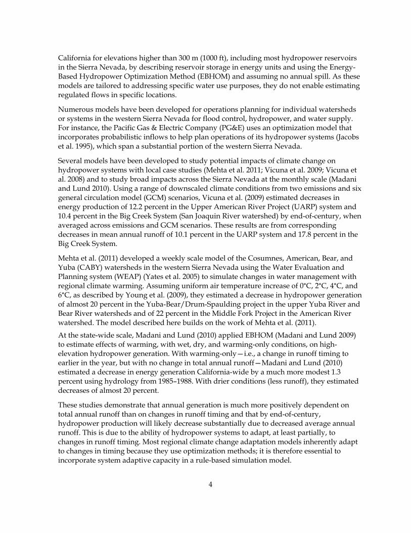
Table 2: Modeled Features and Attributes

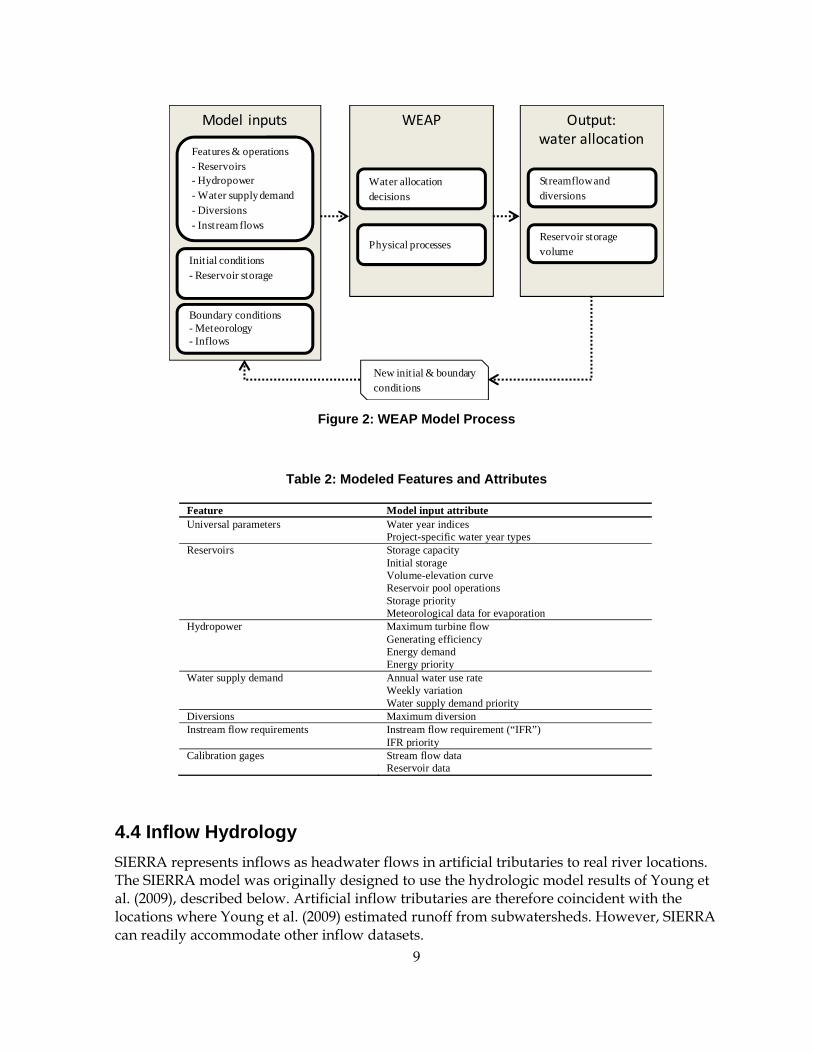
4.4 Inflow Hydrology

SIERRA represents inflows as headwater flows in artificial tributaries to real river locations. The SIERRA model was originally designed to use the hydrologic model results of Young et al. (2009), described below. Artificial inflow tributaries are therefore coincident with the locations where Young et al. (2009) estimated runoff from subwatersheds. However, SIERRA can readily accommodate other inflow datasets.

Model  inputs WEAP Output:water allocation

Reservoir storage volume

Streamflow and diversions

Water allocation decisions

Initial conditions- Reservoir storage

Boundary conditions- Meteorology- Inflows

Features & operations- Reservoirs- Hydropower- Water supply demand- Diversions- Instream flows

New initial & boundary conditions

Physical processes

Feature Model input attributeUniversal parameters Water year indices

Project-specific water year types Reservoirs Storage capacity

Initial storage Volume-elevation curve Reservoir pool operations Storage priority Meteorological data for evaporation

Hydropower Maximum turbine flow Generating efficiency Energy demand Energy priority

Water supply demand Annual water use rate Weekly variation Water supply demand priority

Diversions Maximum diversion Instream flow requirements Instream flow requirement (“IFR”)

IFR priority Calibration gages Stream flow data

Reservoir data

10

Young et al.(2009) developed a weekly scale hydrologic simulation model of the western Sierra Nevada watersheds using WEAP, assuming no regulating infrastructure. WEAP uses a spatially explicit, one-dimensional, two-soil layer model, which simulates surface runoff and other hydrologic responses by explicitly accounting for overland flow, snow accumulation and melt, soil moisture storage, and evapotranspiration (Yates et al. 2005). Young et al. (2009) divided each watershed into subwatersheds, defined by locations—called “pour points”—of management interest or where there was sufficient observed data. They intersected each subwatershed with 250-meter (m) elevation bands, resulting in “catchments” that each have homogeneous physical characteristics such as meteorological conditions, soil conditions, and mix of land use cover.

Using weekly time steps, Young et al. (2009) modeled twenty-one water years (1980–2001) using interpolated Daymet climate data for historical precipitation, air temperature, and vapor pressure deficits. Watersheds were characterized using U.S. Geological Survey (USGS) 10 m digital elevation models (DEM), soil surveys from the Natural Resource Conservation Service (NRCS), and land cover from the USGS National Land Use Classification Database (NLCD). Simulated flows were calibrated at unregulated stream flow locations using data from USGS stream gages, and at some regulated sites using estimates of unimpaired hydrology from the California Department of Water Resources (DWR).

The unimpaired runoff models were calibrated for monthly flows at the outlets of 13 of the 15 watersheds—the Bear River and Calaveras River watersheds were omitted for lack of observed data—and for snow water equivalent (SWE) at 15 high-elevation locations (Young et al. 2009). This is an important consideration when assessing model results, which are sensitive to boundary inflows.

The model is also applied using runoff from a variable infiltration capacity (VIC) model. The VIC-based hydrologic model, described by Maurer et al. (2002), spans the North American continent and uses cells that span of 1/8° longitudinal and latitudinal dimensions. Variable infiltration capacity runoff is at the daily time step. Runoff from the VIC model was prepared for use in SIERRA by intersecting the 1/8° cells with WEAP subwatersheds using ArcGIS v9.3. Contributing VIC runoff was summed across intersected areas, weighted by proportion of intersected area to total subwatershed area. Daily runoff was aggregated to the weekly scale.

4.5 Universal Parameters

Universal parameters, called “key assumptions” in WEAP, can be used across the physical or management domain as primary or intermediary parameters to simplify expressions. For example, instream flow requirements often depend on a Water Year Type (WYT) that is regional in scope rather than associated with a single managed feature. A WYT defined as a key assumption can be used in operating rules for several instream flow requirement locations. Key assumptions are discussed as needed below, primarily for hydropower generation and instream flow requirements.

11

4.6 Reservoirs

Storage Capacity Reservoir storage capacities were mostly obtained directly from the California Data Exchange Center (CDEC) and are listed in Appendix A.

Initial Storage The beginning of the modeling period is October 1, 1980. Initial storage values were mostly from CDEC, but also from USGS gauges. Where only monthly reservoir storage data were available, storage values from October 1980 are used, as storage values from CDEC are for beginning-of-month. Where daily reservoir storage data were available, storage values from on October 1, 1980, were used. If historical storage was unavailable for October 1980, and a relationship between previous water year type and October storage was observed, then the average October storage for Wet water years on record was used, since Water Year 1980 was Wet under both the Sacramento and San Joaquin Valley Water Year Type definitions. If no relationship between water year type and October storage was apparent, then a simple average of storage levels for all Octobers on record was used, rounded to the nearest 100 AF.

Volume-Elevation Curves Volume-elevation data for most reservoirs are from annual reservoir reports published by the U.S. Geological Survey. For reservoirs where such reports did not exist or did not include volume-elevation data, volume-elevation curves were created using a second-order polynomial fit using historical volume and elevation data reported by CDEC. Mountain Meadows Reservoir (North Fork Feather River) had neither a USGS report nor historical volume and elevation data from CDEC; a linear volume-elevation curve for this reservoir was assumed. Linear volume-elevation curves were also used for many small reservoirs.

Reservoir Zone Operations Reservoir operations for recreation, water supply, and flood control are defined by setting requisite volumes for the inactive zone, buffer zone, and conservation zone of reservoirs (“zones” are also known as “pools”).

Inactive zone – The inactive zone of a reservoir is the level, in elevation or storage, below which water cannot be withdrawn, for physical or operational reasons. An inactive zone storage volume was included for most reservoirs based on observed historical minimum levels.

Buffer zone – The buffer zone is the volume or elevation below which water allocations are curtailed, but not ceased. To help guide reservoir operations during the refill (wet season) period, an increasing buffer zone was defined in some reservoirs during a defined refill period.

Conservation and flood zones – The conservation zone is the volume available to store water above the inactive and buffer zones to meet downstream demand. A maximum conservation zone level, or rule curve, is used to create flood space in flood control reservoirs. Rule curves were included for New Bullards Bar Reservoir (North Fork Yuba River), and Lake Isabella (Kern River), though were not fully developed. Some non-flood control reservoirs were

12

assigned conservation zone rule curves based on known operational objectives from public documents.

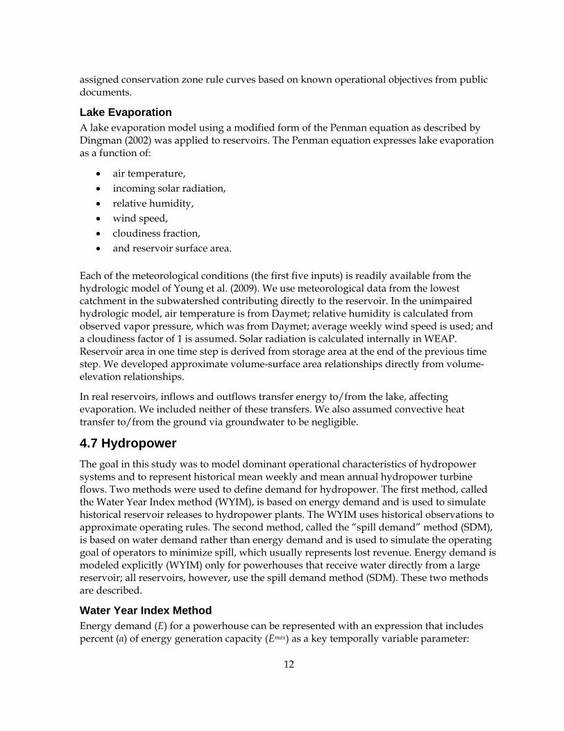
Lake Evaporation A lake evaporation model using a modified form of the Penman equation as described by Dingman (2002) was applied to reservoirs. The Penman equation expresses lake evaporation as a function of:

air temperature, incoming solar radiation, relative humidity, wind speed, cloudiness fraction, and reservoir surface area.

Each of the meteorological conditions (the first five inputs) is readily available from the hydrologic model of Young et al. (2009). We use meteorological data from the lowest catchment in the subwatershed contributing directly to the reservoir. In the unimpaired hydrologic model, air temperature is from Daymet; relative humidity is calculated from observed vapor pressure, which was from Daymet; average weekly wind speed is used; and a cloudiness factor of 1 is assumed. Solar radiation is calculated internally in WEAP. Reservoir area in one time step is derived from storage area at the end of the previous time step. We developed approximate volume-surface area relationships directly from volume-elevation relationships.

In real reservoirs, inflows and outflows transfer energy to/from the lake, affecting evaporation. We included neither of these transfers. We also assumed convective heat transfer to/from the ground via groundwater to be negligible.

4.7 Hydropower

The goal in this study was to model dominant operational characteristics of hydropower systems and to represent historical mean weekly and mean annual hydropower turbine flows. Two methods were used to define demand for hydropower. The first method, called the Water Year Index method (WYIM), is based on energy demand and is used to simulate historical reservoir releases to hydropower plants. The WYIM uses historical observations to approximate operating rules. The second method, called the “spill demand” method (SDM), is based on water demand rather than energy demand and is used to simulate the operating goal of operators to minimize spill, which usually represents lost revenue. Energy demand is modeled explicitly (WYIM) only for powerhouses that receive water directly from a large reservoir; all reservoirs, however, use the spill demand method (SDM). These two methods are described.

Water Year Index Method Energy demand (E) for a powerhouse can be represented with an expression that includes percent (α) of energy generation capacity (Emax) as a key temporally variable parameter:

13

m axt tE E (0)

Energy generation capacity (Emax) is assumed constant in all high-head hydropower plants, such that:

max maxE h Q (0)

where γ is the specific weight of water, h is fixed hydropower head, η is plant efficiency (assumed 90 percent), and Qmax is the hydropower turbine flow capacity. The purpose of the energy demand modeling method is to define αt. The Water Year Index method (WYIM) does this by relating weekly hydropower demand to annual water availability as a coarse approximation of actual demand.

Mehta et al.(2011) demonstrated that mean weekly hydropower operations can be adequately represented by establishing a relationship between water year type (WYT) and water demand for hydropower during any given week. For each week and each powerhouse, Mehta et al. (2011) used three regional water year types (dry, normal, and wet) and determined the respective non-exceedance percentiles of historical hydropower turbine for that week. A single non-exceedance percentile value was then chosen to specify a minimum diversion amount during simulation. For example, for a particular week, hydropower turbine flow demand might be the 10 percent non-exceedance value of historical flows for that week in dry years, 50 percent non-exceedance in normal years, and 90 percent non-exceedance in wet years. Mehta et al. (2011) adjusted these values during calibration.

The Water Year Index method (WYIM) modifies this approach. The WYIM assumes a continuous, linear response of turbine flow to regional water availability, as defined by a water year index, instead of the discrete, non-linear response to water year types of the CABY model.

For each week and each powerhouse, a linear relationship between water year index (WYI)—a continuous function of regional mean annual runoff—and hydropower turbine flow is established using historical observations. The equation parameters of the resulting linear fit—slope and intercept—are then used to determine hydropower turbine flow demand percent (α) given WYI:

t tt max

m WYI b

Q

(0)

where mt is the slope of the line, bt is the intercept during week t for any given powerhouse, and Qmax is the maximum turbine capacity. In implementation, (5) is modified as needed to ensure that 0 ≤ αt ≤ 1.

The slope and intersect of Eq. (0) are readily determined from historical data and WYI for each powerhouse. For pumped storage facilities, which can have reverse flows, Eq. (0) is used without modification.

14

In the SIERRA model, the California Department of Water Resources (DWR) Sacramento Valley WYI was used for the northern watersheds (Feather through American) and the San Joaquin Valley WYI was used for the southern watersheds (Mokelumne through Kern). DWR WYIs are continuous and have units of million acre-feet (MAF) per year. The Sacramento Valley WYI is defined as:

WYISacValley = 0.4 * Current Apr-Jul Runoff Forecast (in MAF) + 0.3 * Current Oct-Mar Runoff in (MAF) + 0.3 * Previous Water Year's Index (if the Previous Water Year's Index exceeds 10.0, then 10.0 is used) (CDEC, 2010)

where “Runoff” is the sum of runoff from Sacramento River at Bend Bridge, Feather River inflow to Lake Oroville, Yuba River at Smartville, and American River inflow to Folsom Lake (CDEC 2010). The latter three can be computed directly from the unimpaired hydrologic models. To include the Sacramento River, we used a simple linear regression to correlate monthly flows in the Sacramento River at Bend Bridge with historical monthly Full Natural Flow (FNF) calculated by DWR for the Feather River. Using linear regression results, and assuming no change in relationship between the flows with warming, we calculated monthly Sacramento River flows for each climate warming scenario using simulated Feather River flows.

The San Joaquin WYI is defined as:

WYISJValley = 0.6 * Current Apr-Jul Runoff Forecast (in MAF) + 0.2 * Current Oct-Mar Runoff in (MAF) + 0.2 * Previous Water Year's Index (if the Previous Water Year's Index exceeds 4.5, then 4.5 is used) (CDEC 2010)

where “Runoff” is the sum of Stanislaus river inflow to New Melones reservoir, Tuolumne river inflow to New Don Pedro reservoir, Merced river inflow to Lake McClure, and San Joaquin river inflow to Millerton Lake, each of which is available from the unimpaired hydrologic models (CDEC 2010).

WYISacValley and WYISJValley are calculated for each atmospheric warming scenario using simulated runoff for the scenario. Since each WYI depends partly on WYI from the previous year, an initial WYI is required. To do this for warming scenarios, we established a linear regression between ΔT and WYT for each water year in the study period (i.e., WY 1981–2000). The slope of that linear relationship from a year with a WYI historically similar to that of WY 1980 was used to estimate WYI for WY 1980 for each warming scenario. Because initial rough estimates of WYI for WY 1980 were needed to determine the WYI-ΔT slopes, we excluded the first four Water Years from the slope calculations to eliminate the lag influence of WYI from one year to the next.

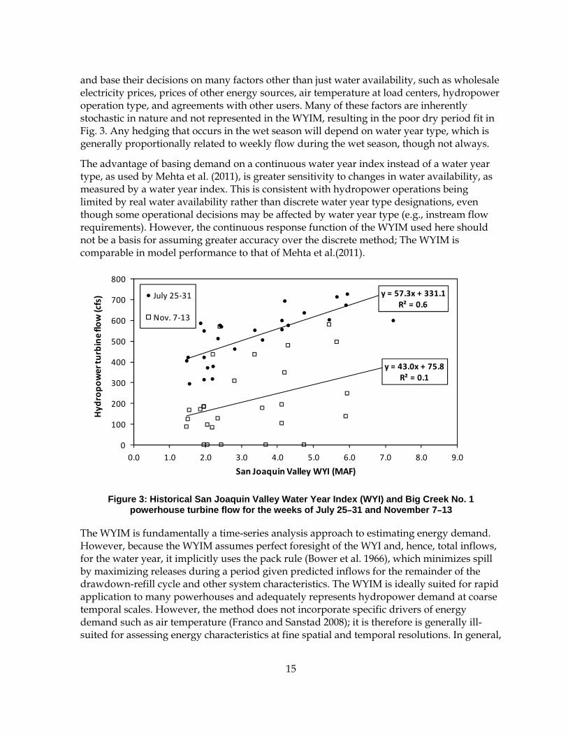
Figure 3 demonstrates this method, including its strengths and inherent limitations. Figure 3 shows relationships between the San Joaquin Valley WYI and hydropower turbine flow for Big Creek No. 1 powerhouse (San Joaquin watershed) for two weeks of the year: July 25–31 and November 7–13.As with most powerhouses, the linear relationship between WYI and turbine flow is stronger in wetter weeks when the reservoirs are full (e.g., July) and weaker during drier weeks, when reservoirs are empty (e.g., November). In wet weeks, hydropower and other uses can generally take as much as is available, even in drier years (Figure 3). During dry weeks, however, water users must be more selective about when they use water

15

and base their decisions on many factors other than just water availability, such as wholesale electricity prices, prices of other energy sources, air temperature at load centers, hydropower operation type, and agreements with other users. Many of these factors are inherently stochastic in nature and not represented in the WYIM, resulting in the poor dry period fit in Fig. 3. Any hedging that occurs in the wet season will depend on water year type, which is generally proportionally related to weekly flow during the wet season, though not always.

The advantage of basing demand on a continuous water year index instead of a water year type, as used by Mehta et al. (2011), is greater sensitivity to changes in water availability, as measured by a water year index. This is consistent with hydropower operations being limited by real water availability rather than discrete water year type designations, even though some operational decisions may be affected by water year type (e.g., instream flow requirements). However, the continuous response function of the WYIM used here should not be a basis for assuming greater accuracy over the discrete method; The WYIM is comparable in model performance to that of Mehta et al.(2011).

Figure 3: Historical San Joaquin Valley Water Year Index (WYI) and Big Creek No. 1

powerhouse turbine flow for the weeks of July 25–31 and November 7–13

The WYIM is fundamentally a time-series analysis approach to estimating energy demand. However, because the WYIM assumes perfect foresight of the WYI and, hence, total inflows, for the water year, it implicitly uses the pack rule (Bower et al. 1966), which minimizes spill by maximizing releases during a period given predicted inflows for the remainder of the drawdown-refill cycle and other system characteristics. The WYIM is ideally suited for rapid application to many powerhouses and adequately represents hydropower demand at coarse temporal scales. However, the method does not incorporate specific drivers of energy demand such as air temperature (Franco and Sanstad 2008); it is therefore is generally ill-suited for assessing energy characteristics at fine spatial and temporal resolutions. In general,

y = 57.3x + 331.1R² = 0.6

y = 43.0x + 75.8R² = 0.1

0

100

200

300

400

500

600

700

800

0.0 1.0 2.0 3.0 4.0 5.0 6.0 7.0 8.0 9.0

Hyd

ropower turbine flo

w (cfs)

San Joaquin Valley WYI (MAF)

July 25‐31

Nov. 7‐13

16

this method and that of Mehta et al. (2011) are intended to estimate average abstractions for hydropower flows rather than simulate actual operations in any given week.

Another important inherent limitation in the WYIM is that the timing of energy demand timing is fixed, based on the historical timing of releases. However, the historical timing of releases is based, in part, on the historical timing of inflows. The WYIM fails to account for the change in timing of flows caused by warming. For the same total annual runoff, greater winter precipitation-driven runoff from warming causes more frequent spills in the winter using the WYIM. For a given WYI, this method does not increase hydropower generation even if water is spilling. This is resolved with the spill demand method described below.

Spill Demand Method To prevent hydropower demand at less than capacity when a reservoir is spilling, another hydropower operating rule is introduced, called the spill demand method (SDM). The SDM simply requires that any inflow in excess of existing demands be diverted to generate hydropower. This ensures that hydropower plants use, as much as possible, water that cannot be stored and that would otherwise spill. The SDM is expressed mathematically as:

sd in max target rr

Q Q S S Q Q (0)

where Qsd is the hydropower release in excess of the target release, Qin is the inflow during the week, Smax is the reservoir capacity, S is the reservoir storage, Qtarget is the target release to meet energy demand (e.g., as determined by the WYIM), and Qr is release for all other

purposes. Qsd is constrained by 0 ( )sd max targetQ Q Q . This is similar to the pack rule

(Bower et al. 1966), though the SDM minimizes spill during the current time step only, without consideration of future inflows. Implementing the SDM mathematically is challenging, since many of the independent variables (storage level, inflow, and releases) are not known until the water allocation problem of the current time step has already been solved. The SDM is applied in SIERRA with an additional demand of 100 percent of turbine flow capacity, with a demand priority lower than upstream facilities and other local uses, if any, including meeting energy demand using the WYIM.

The SDM is applied to all powerhouses to minimize spill, which is lost energy/revenue. There are three distinct situations where this method is useful for hydropower generation. First, this method is applied to hydropower plants that lack upstream storage (i.e., off-stream run-of-river plants), such as in the Kaweah and Tule watersheds. This rule ensures that the plant diverts as much as possible, constrained only by IFRs and facility capacities. Second, this method is applied to powerhouses operated in coordination with upstream facilities. In high-elevation hydropower systems, hydropower plants are typically configured as a series as high-head plants, with water diverted via artificial channels to maintain maximum head before release via a penstock. Lower elevation plants in such cases demand 100 percent of capacity, albeit with a lower priority than upstream facilities. This method will result in de facto coordinated operations. Finally, this method is applied to all peaking powerplants, with a hydropower priority lower than all other local priorities. This ensures that any spill—i.e., water not stored or purposefully released to meet multiple demands—is diverted for

17

hydropower generation, within capacity limitations. The latter use of the SDM is particularly important when considering climate warming, as it guarantees that peaking facilities utilize any extra available water rather than limiting diversions to historical patterns.

4.8 Water Supply Demand

Water supply for urban and agriculture use is limited in most of the Sierra Nevada above the large low-elevation, multi-purpose reservoirs and is small relative to water supply for agriculture in the Central Valley. However, they can be important because they have a higher priority than hydropower generation and play a central role in some systems (e.g., the Hetch Hetchy system in the Tuolumne, among others). When water is scarcer in drier years or in warming scenarios, hydropower is reduced before water supply if there is a conflict.

Demands were generally fixed, regardless of water year type, based on historical mean weekly flows, using data provided by water agencies. A major exception is diversions for water supply to San Francisco from the Hetch Hetchy system (Tuolumne River watershed). Analysis of historical diversions to San Francisco indicated a strong negative correlation between San Joaquin Valley WYI and annual diversions to San Francisco. This trend was confirmed in a private conversation with the San Francisco Public Utilities Commission (SFPUC), who noted that the Raker Act of 1913, which governs the Hetch Hetchy system, requires SFPUC to prioritize local sources of water. Thus, in wetter years, demand for diversions from the Tuolumne River watershed decreases. The smallest demand modeled was the Crab-Aiken Ditch Co. in the Tule River watershed, with a maximum diversion of 6.5 cubic feet per second (cfs). Some other more substantial demands exist but are excluded for lack of sufficient understanding of diversion rules (e.g., water supplied by the Utica Power Authority from the Stanislaus River). A complete list of modeled water supply demand locations is included in Appendix A.

4.9 Instream Flow Requirements

Instream flow requirements (IFRs) in WEAP consist of minimum instream flows (MIFs) required below dams and diversions. We included all IFRs identified in Federal Energy Regulatory Commission (FERC) licenses or from other documents if the project was not regulated by FERC (e.g., the Hetch Hetchy system). We did not include pulse flows, which some projects require to flush sediment downstream, or releases for whitewater recreation.

Instream flow requirements range from a single fixed value to values that vary by month and by water year type. IFRs that vary by month require a day-to-week conversion for month beginning and end dates. In general, we converted 30-day months to 4 weeks and 31-day months to 5 weeks. Some IFRs depend on the current state of system variables other than water year type. For example the IFR below Hetch Hetchy reservoir depends on cumulative precipitation at O’Shaughnessy Dam until the month of July, when it depends on inflow to Hetch Hetchy Reservoir. For these IFRs we used values calculated in the previous time step to determine the appropriate IFR for the current time step. Appendix A lists all IFR locations.

We calculated water year types (WYT) as needed for development of IFR expressions using simulated unimpaired flows from the inflow datasets. Water year type definitions are

18

usually specific to a given hydroelectric project. Definitions can further vary within a project, such as for different IFR locations within the project. Some operations may also use spatially broader water year types such as the Sacramento and San Joaquin Valley WYT. Since water year types mostly depend on streamflow and flows change with climate changes, climate change affects operations constrained by water year types.

All water year type definitions use a combination of year-to-date flows and flow forecasts for the remainder of the water year. IFRs below Hetch Hetchy additionally depend on accumulated precipitation. For expediency, we computed water year types assuming perfect knowledge of the water year type using the unimpaired hydrology data, without forecasting. Future model improvements should include incorporating forecasting for water year type definitions and other operations.

4.10 Diversions

We included maximum diversion capacity for all diversions and assumed these to be constant over time. Maximum diversion values were obtained from a variety of publicly available documents, primarily hydropower license documents. When a maximum diversion was not available from a document, maximum flow from gage data was used. In many instances, maximum diversion values and maximum turbine flows were redundant. In the CABY region, the discrete minimum flow requirement method implemented by Mehta et al.(2011)was retained for diversions not directly leading to a hydropower plant. A list of all diversions is included in Appendix A.

4.11 Priority Setting

Correctly setting priorities is crucial for accurate results in priority-based water resources management models. In WEAP, priorities are assigned to all water management purposes, including for instream flow requirements, water supply, hydropower, and reservoirs. Priorities can range from 1 to 99, where 1 represents the highest priority. We assigned priorities to each feature based on (1) location of the feature in relation to other features and (2) the feature type, with modifications as needed. We did this by developing a two-digit priority scheme, where the first digit is based on the feature’s location and the second digit based on the feature type. Feature locations were generalized by grouping them by hydropower or other development project. Upstream features/projects were assigned higher priorities (lower numbers), while downstream features/projects were assigned lower priorities. Without this upstream/downstream priority assignment scheme, the model allocates water to downstream users with high priorities (e.g., a utility district) instead of allowing a lower priority upstream user to use the water first.

Features were assigned priorities based on general water rights priorities:

1. Instream flow requirements 2. Water supply demand 3. Hydropower 4. Reservoirs

Hydropower facilities immediately below a reservoir, which used the WYIM to establish fixed energy demand, were assigned a priority equal to the reservoir. This worked because

19

demand was based on historical observations. However, lower elevation hydropower plants in the same hydropower chain received a lower priority, as discussed above. Table 3 shows priorities for a hypothetical two-project system with each feature type represented in each project. Since allocating water among different potential uses is fundamentally driven by priority, the model is generally more sensitive to priorities than any other model parameter. Though this scheme works generally, in practice each water system is unique, necessitating a more detailed assessment of local priorities for future model improvements. Some priorities were adjusted as needed during model calibration. In particular, some reservoirs were assigned a higher priority during the refill period and a lower priority during the drawdown period.

Table 3: Priority Assignments for Two Hypothetical Projects

Water use type Project location / priority

Upstream Downstream

Instream flow req’t 11 21

Water supply demand 13 23

Hydropower – WYIM 15 25

Hydropower – SDM 19 29

Reservoir storage 15 25

4.12 Interbasin Transfers

We modeled interbasin transfers differently on a case-by-case basis. Generally, an interbasin transfer is simulated in only one of the two watersheds that the transfer saddles, integrating the transfer into the watershed to which the transfer project belongs. In the watershed that does not dominate in the project, inflows to or outflows from that project are assumed based on historical or other modeled data. Several small interbasin transfers were omitted from the model for simplification (e.g., diversions from the Stanislaus to the Calaveras River watersheds).

Since the CABY watersheds are integrated into one model, intra-CABY transfers did not need special consideration. Transfers that did require special consideration include:

Yuba watershed to Feather watershed – Slate Creek provides water to the South Fork Feather River project for hydropower and water supply. The transfer was simulated in the Feather watershed model. Simulated transfers were included as a fixed weekly demand from Slate Creek in the CABY sub-model.

Stanislaus watershed to Tuolumne watershed – Flows from the Stanislaus watershed to the Tuolumne watershed via Phoenix powerhouse are included in the Stanislaus model.

4.13 Integrating Models and Data Management

A significant challenge in developing the model described here was to integrate 12 independent WEAP-based models with multiple climate scenarios for ease in execution, uniformity in output, and rapid results assessment and analysis. We used the Python

20

scripting language to develop a suite of tools to address these needs. These tools can be readily adapted, if needed, and used to easily execute the model with alternative climate warming or other scenarios.

4.14 Climate Change Scenarios

To assess the vulnerability of upper Sierra Nevada water systems to climate warming—with inflow as the primary exposure unit—SIERRA was applied using inflow datasets from two different unimpaired hydrology studies to represent historical-, near-, mid-, and far-term climate conditions (Table 4). The first dataset is from Young et al. (2009), who applied their WEAP hydrologic model with spatially and temporally uniform increases in air temperature of 0°C, 2°C, 4°C, and 6°C and no change in precipitation magnitude or timing. These temperature increases broadly represent anticipated changes in the regional climate over the next 50–100 years, approximating temperature changes from the historical- through far-term (Table 5). Historical precipitation was assumed by Young et al. (2009) because downscaled general circulation models (GCMs) are less consistent in their prediction of changes in magnitude or timing of precipitation in California(Hayhoe et al. 2004).

The second dataset is from a variable infiltration capacity (VIC) hydrologic model for the United States (Maurer et al. 2002). The VIC model was applied using two emissions scenarios (B1 and A2) and the following downscaled climate data from six general circulation models (GCMs): CNRMCM3, GFDLCM21, MIROC32MED, MPIECHAM5, NCARCCSM3, and NCARPCM1. However, CNRMCM3 was omitted due to modeling difficulties with results from this particular dataset, reducing the GCM count to five. In this study, we considered the A2 emissions scenario and all six GCM results. Historical- through far-term climate conditions are represented with different time spans, as indicated in Table 1.

As noted above, historical runoff from the VIC model was found to be unusually high (Rheinheimer et al. 2011). However, derived from downscaled GCMs, the high historical runoff did not affect the climate change vulnerability assessment described here, as vulnerability to climate change was assessed with different precipitation values. Of greater importance here is that in contrast to the WEAP model, the VIC model was not calibrated for the Sierra Nevada. Pending any calibration of the VIC model for the Sierra Nevada, results using the VIC runoff data are of interest for average trends.

Table 4: Representation of Historical and Future Climate Conditions

Time period I. WEAP runoff

scenario II. VIC runoff

scenario

Historical +0°C 1961–1990

Near-term +2°C 2005–2034

Mid-term +4°C 2035–2064

Far-term +6°C 2070–2099

21

Section 5: Calibration and Model Assessment

The parameters and operating rules used in SIERRA were fixed, based on historical observations, so a formal calibration was generally not required. However, priorities, which were assigned initial values as discussed above, required adjustment in some instances to mimic observed system behavior. This was particularly true in cases for reservoirs in series or parallel in complex systems. Also, we observed that relative priorities can change seasonally in some such systems. Calibration was therefore limited to adjusting relative priorities as needed to ensure that reservoirs operated relative to each other as close as possible to observed operations. No adjustments were made to the inflow hydrology dataset. Model improvements for specific systems will require adjusting the physical parameters of the hydrologic model and contacting system operators to better understand and represent operational logic and operating priorities.

Here, we assess model performance using the WEAP-based unimpaired hydrologic model of Young et al. (2009), which was developed specifically for the Sierra Nevada. The VIC hydrologic model (Maurer et al. 2002), which was used for some climate change impact assessments as described below, was not specifically calibrated for the Sierra Nevada and showed a substantial over-estimation of regional runoff compared with the WEAP-based model (Rheinheimer et al. 2011). The historical runoff from the VIC model was therefore unsuitable for use in model performance assessments. Most (86 percent) of the noted discrepancies between historical runoff from the WEAP and VIC models were explained by the unusually high precipitation values in the VIC model.

To assess performance of the model, we focus on powerhouse turbine flow and reservoir storage, as these operations are the most challenging to simulate accurately and because meaningful characterizations of alterations to the natural flow regime—a long term goal—depend on a good understanding of simulation accuracy. Because modeled system behavior is sensitive to the hydrologic model, which was calibrated for flows at the watershed outlets and for snow water equivalent at only 15 high-locations model performance assessments are only considered in the context of watershed-scale or range-scale operations. Limiting model performance assessments to specific facilities is only appropriate with further calibration of the hydrologic model.

To assess model performance, we calculated the following metrics for hydropower turbine flow:

Nash-Sutcliffe model efficiency (NSME) at the seasonal and annual scales Root mean square error (RMSE) at the seasonal and annual scales Mean bias

We also compare mean total and mean seasonal observed and simulated hydropower turbine flow, energy generation, and reservoir storage as points in a scatter plot at the range and watershed scales.

The Nash-Sutcliffe model efficiency index NSME(Nash and Sutcliffe 1980), also called the coefficient of determination (R2) in other contexts, is often used in hydrology studies to

22

compare modeled flows to observations. Though useful, NSME alone is not a reliable metric of model predictive power, as discussed by Jain and Sudheer (2008).NSME is defined as:

2

, ,1

2

,1

1

T

o t m tt

T

o t ot

Q QNSME

Q Q

(0)

where ,o tQ and

,m tQ are the observed and modeled flows, respectively, at time t, and T is the

total number of observations. The Nash-Sutcliffe index describes the percentage of the variance that can be explained by the model. E can range from –∞ to 1. When E = 1, the model accurately predicts the observations; when E = 0, the model is no better or worse than the mean of the observations; when E< 0, the model is a worse predictor than the mean of the observations. Values typically become asymptotic as they approach 1 (perfect predictive power), thus large negative values should not be interpreted as equally nearing imperfection.

Root mean square error (RMSE) is a measure of the spread of the differences between observed and modeled data points. RMSE is defined as:

2, ,

1

( )1

m t o tt

T

RMSE xT

x

(0)

where t is the time step and T is the total number of time steps. RMSE is always positive and smaller values indicate that modeled values are consistently closer to observed values. As with NSME, RMSE changes with time step length. Here, RMSE is normalized by dividing Eq. (5) by the mean observed flow, such that units are in percent.

Mean bias (mBias) quantifies the difference between the mean of modeled values and the mean of observed values:

, ,1 1

1 T T

m t o tt t

mBias x xT

(0)

Mean bias can be either positive or negative; values closer to zero indicate greater model accuracy of mean modeled flows. As with RMSE, here mean bias is normalized to mean observed flow, resulting in percent units.

5.1 Hydropower Turbine Flow

Table 5 lists hydropower turbine flow model performance metrics at multiple temporal scales. 78 of the 86 fixed head hydropower plants are included in the performance assessment, as eight plants lacked sufficient observed data to make meaningful comparisons. At all temporal scales (weekly, seasonal, annual mean flow), approximately 60 percent of modeled plants have NSME values greater than zero, indicating most are better represented with the simulation model than with their historical mean flow. More than half have NSME

23

values of 0.13, 0.18, and 0.31 at the weekly, seasonal, and annual scales, respectively (Table 5). Model simulation results improve with coarser units of analysis. The most well-modeled hydropower plants are also the ones with the greatest historical diversions (Figure 4) and the greatest hydropower generation. Conversely, the least well-modeled plants are smaller (Figure 4). Most plants under-represent hydropower turbine flow, with a median normalized mean bias of -12 percent. The mean normalized mean bias is approximately -10 percent. These results indicate that the more important hydropower plants are simulated well.

Table 5: Model Performance Metrics for Fixed Head Hydropower Turbine Flow

Figure 4: Seasonal NSME by Mean Modeled Turbine Flow

Figure 5 compares observed and modeled mean hydropower turbine flow in aggregate and by season (log scale). Each point in Figure 5 represents a single powerhouse. On average, mean hydropower flows match mean observed flows closely, though there is a tendency of the model to slightly under-predict flows, with a slope of 0.98 for mean annual flow. This is consistent with the negative mean bias noted above. The model tends to under-represent flows in the summer (July, August, September or JAS) and fall (October, November, December or OND), with modeled flows at 86 percent and 88 percent of observed flows, respectively. By contrast, flows are slightly over-represented in winter (January, February, March or JFM) and spring (April, May, June or AMJ), with modeled flows 103 percent and 112 percent of observed flows, respectively.

Percentile

WeeklyNSME (%)

SeasonalNSME (%)

AnnualNSME (%)

SeasonalRMSE (%)

AnnualRMSE (%)

meanbias (%)

100% (maximum) 0.76 0.80 0.92 12.88 6.06 1.2875% 0.38 0.50 0.63 3.27 1.21 0.0050% (median) 0.13 0.18 0.31 2.56 0.88 -0.1225% -0.31 -0.55 -0.69 1.82 0.60 -0.230% (minimum) -4.79 -7.79 -89.87 0.69 0.00 -0.70

‐9

‐8

‐7

‐6

‐5

‐4

‐3

‐2

‐1

0

1

2

0 10 20 30 40 50 60 70

NSME

Hydropower turbine flow (m3/s)

24

Similarly, Figure 6 compares observed and modeled mean hydropower generation in aggregate and by season. The model generally under-predicts hydropower generation, to a slightly greater degree than hydropower turbine flow. Figure 7 shows that the model effectively simulates historical total regional hydropower generation at the seasonal scale during the study period. However, consistent with the seasonal energy comparison results of Figure 6b, simulated energy is typically lower than observed during the summer, fall, and spring.

Figure 5: Observed and Modeled Mean Annual and Seasonal Hydropower Turbine Flow

25

Figure 6: Observed and Simulated Mean Annual and Seasonal Hydropower Generation

Figure 7: Total Observed and Modeled Hydropower Generation

These assessment results indicate that the model effectively represents observed hydropower turbine flow and generation patterns and that the model can be used to assess regional and weekly, seasonal or annual time step responses to changing external drivers such as inflow hydrology. Watershed-scale assessments can be made at the seasonal or annual scale. Change response assessments for specific facilities or systems are possible for approximately one-half of the systems in the Sierra Nevada. Further improvements are needed to more accurately represent specific facilities, particularly many smaller facilities. As the model is

26

responsive to inflow hydrology, improvements in facility operations logic needs to be coupled with improvements in representation of inflow hydrology to better simulate historical operations.

5.2 Reservoir Storage and Evaporation

On average, modeled reservoir storage volumes (Figure 8) are generally modeled slightly more consistently well than hydropower flow or generation at both long term and by season. As with observed hydropower turbine flow, mean storage most closely matches observed values in the spring, when reservoirs are typically relatively full.

Figure 8: Observed and Modeled Mean Annual and Seasonal Reservoir Storage

The California Data Exchange Center does not typically report reservoir evaporation for high elevation reservoirs. One exception is Lake Almanor (Feather River watershed), for which “observed” monthly reservoir evaporation is estimated by using a constant pan evaporation coefficient of 0.7. To assess the lake evaporation model, we applied the model to Lake Almanor using observed reservoir storage. The model simulates the majority of the lake evaporation reported by CDEC, though tends to be lower than reported during late summer through winter and higher during spring and late summer (Figure 9).

27

Figure 9: Mean (WY1981–2000) Mean Lake Evaporation for Lake Almanor Using Observed (CDEC) and Modeled Storage Data

0.0

1.0

2.0

3.0

4.0

5.0

J F M A M J J A S O N D

Evaporation (million m

3/w

eek)

CDEC

Modeled

28

Section 6: Results with Warming

Results from each of the runoff datasets used (WEAP and VIC), as described above, are discussed. Results from the WEAP model runoff are given much more detailed consideration, as the WEAP model was calibrated for the Sierra Nevada. General results are discussed for the VIC runoff scenario set. Using VIC runoff data, we performed basic quantitative assessments of results to identify the vulnerability (exposure) of hydropower generation on a system-wide and watershed basis.

6.1 WEAP Runoff Scenarios: Air Temperature Increase

Total Hydropower Generation

Trends at the weekly time step are important to understand coarser resolution trends. Figure 10 shows total mean weekly hydropower generation and generation changes with +0°C, 2°C, 4°C, and 6°C warming. Warming decreases the total regional mean weekly hydropower generation compared to the historical climate beginning in mid-April, when there is consistently very little change. Mean weekly generation decreases considerably thereafter—by about 40 percent in mid-June with 6°C warming—until late November. Mean weekly generation consistently increases between early December and mid-April, with a maximum increase of about 30 percent in late February with 6°C warming.

Sierra-wide seasonal changes are listed in Table 6 and shown in Figure 11. Hydropower generation increases substantially during the winter, with equally great reductions in generation in the summer. Additional reductions in the other seasons cause a net reduction in mean annual hydropower generation. With 6°C warming, which represents possible end-of-century climate conditions, hydropower generation decreases by almost 1,500 GWh or 7.8 percent compared to historical climate conditions. These results are less than the results of others, discussed above. For example, Vicuna et al. (2009) estimated end-of-century generation losses of 12.2 percent and 10.4 percent for the Upper American River Project (American River) and Big Creek System (San Joaquin River), respectively. However, as discussed below, results for specific watersheds are substantially different from existing local studies.

29

Figure 10: Mean Total Weekly Energy Generation with Warming

Table 6: Seasonal and Annual Hydropower Generation Change with Warming

Generation Warming

OND(Fall)

JFM(Winter)

AMJ(Spring)

JAS(Summar) Annual

+0 °C 3,104 4,331 6,701 4,734 18,870

+2 °C 3,042 4,903 6,430 4,187 18,561

+4 °C 2,974 5,323 5,983 3,690 17,971

+6 °C 2,912 5,640 5,517 3,332 17,401

+0 °C -- -- -- -- --

+2 °C -62 571 -270 -547 -308

+4 °C -130 992 -717 -1,044 -899

+6 °C -192 1,309 -1,184 -1,402 -1,469

+0 °C -- -- -- -- --

+2 °C -2.0% 13.2% -4.0% -11.6% -1.6%

+4 °C -4.2% 22.9% -10.7% -22.0% -4.8%

+6 °C -6.2% 30.2% -17.7% -29.6% -7.8%

Total (GWh)

Change (GWh)

Change (%)

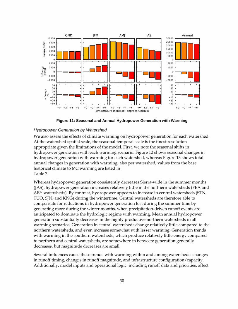
30

Figure 11: Seasonal and Annual Hydropower Generation with Warming

Hydropower Generation by Watershed

We also assess the effects of climate warming on hydropower generation for each watershed. At the watershed spatial scale, the seasonal temporal scale is the finest resolution appropriate given the limitations of the model. First, we note the seasonal shifts in hydropower generation with each warming scenario. Figure 12 shows seasonal changes in hydropower generation with warming for each watershed, whereas Figure 13 shows total annual changes in generation with warming, also per watershed; values from the base historical climate to 6°C warming are listed in Table 7.

Whereas hydropower generation consistently decreases Sierra-wide in the summer months (JAS), hydropower generation increases relatively little in the northern watersheds (FEA and ABY watersheds). By contrast, hydropower appears to increase in central watersheds (STN, TUO, SJN, and KNG) during the wintertime. Central watersheds are therefore able to compensate for reductions in hydropower generation lost during the summer time by generating more during the winter months, when precipitation-driven runoff events are anticipated to dominate the hydrologic regime with warming. Mean annual hydropower generation substantially decreases in the highly productive northern watersheds in all warming scenarios. Generation in central watersheds change relatively little compared to the northern watersheds, and even increase somewhat with lesser warming. Generation trends with warming in the southern watersheds, which produce relatively little energy compared to northern and central watersheds, are somewhere in between: generation generally decreases, but magnitude decreases are small.

Several influences cause these trends with warming within and among watersheds: changes in runoff timing, changes in runoff magnitude, and infrastructure configuration/capacity. Additionally, model inputs and operational logic, including runoff data and priorities, affect

31

system responses to change. Each influence is described, though a full sensitivity analysis was beyond the scope of this work.

First, throughout the Sierra Nevada there is less snowmelt-driven runoff in the late spring and early summer and greater precipitation-driven events in the winter. Even with no change in overall runoff, as this shift from snowmelt-driven events to earlier precipitation-driven events occurs, runoff becomes more evenly distributed throughout the year. Hydropower systems benefit from this increased uniformity in the near- and mid-term (+2 and 4°C) by being able to capture more incoming water, and spilling less. Thus, the timing of runoff has a major effect on system response to warming. Hydropower generation with greater warming (+6°C) is also influenced by changes in runoff timing, but in most cases changes in runoff magnitude dominate other influences. The combined effects of a shift to higher precipitation-driven events (high winter flows) and reduced total annual runoff results in greater earlier spill and reduces overall water available for hydropower generation. To benefit or minimize losses from changes in runoff timing and magnitude, however, the system has to be configured and operated to allow for flexibility in operations and there has to be enough existing under-utilized hydropower capacity in earlier weeks.

Figure 12: Seasonal Hydropower Generation Change by Watershed

32

Figure 13: Mean Annual Hydropower Generation Change by Watershed

Table 7: Mean Annual Hydropower Generation Change with +6°C Warming by Watershed

Finally, limitations of the model itself, including boundary conditions and operation logic, contribute to the observed trends in changes with warming for any particular system. The hydrologic model used was calibrated to watershed outlets and a few snow gauge locations (Young et al. 2009), resulting in poorly simulated runoff in some locations within watersheds. As hydropower systems divert water from specific locations within watersheds, the quality of inflow hydrology simulation at the subwatershed scale affects the quality of system responses to warming. Under-represented inflow to a reservoir, for example, could give that reservoir more capacity to be able to compensate for changes in runoff timing.

Basin

+0 °C(GWh/year)

+6 °C(GWh/year)

Change(GWh/year)

Change(%)

FEA 3,827 3,392 -435 -11.4%

ABY 5,736 4,889 -847 -14.8%

MOK 693 625 -68 -9.7%

STN 918 899 -19 -2.1%

TUO 1,256 1,261 6 0.5%

SJN 4,267 4,311 44 1.0%

KNG 1,476 1,396 -79 -5.4%

KAW 55 48 -7 -12.7%

TUL 38 35 -2 -5.9%

KRN 605 543 -62 -10.3%

Total 18,870 17,401 -1,469 -7.8%

33

Though inflow hydrology is poorly represented in several locations, this did not appear to be a major cause of watershed-wide trends observed in Figures 12 and 13. Operational logic also affects system response to changing inflows, but was less of an issue than other influences.

The unique combination of each influence discussed above affects the response of any particular facility, system, or watershed to climate warming. Assuming the model is accurate, with correct operational logic and input data, the combination of system configuration, runoff magnitude, and runoff timing determine how the system behaves with historical climate and how the system responds to changes with warming. Thus, in the ABY region, substantial decreases in runoff magnitude dominate (Null et al. 2010), such that any existing additional capacity in regional systems is insufficient to substantially accommodate changes due to warming. By contrast, existing infrastructure configuration and capacity in the San Joaquin watershed, combined with minimal decreases in runoff magnitude (Null et al. 2010) with warming allows for minimal loss—gain, even—with warming. Specifically, Mammoth Pool Reservoir and powerhouse (San Joaquin River), which is historically well under capacity most of the year, can take advantage of a shift in runoff timing to reduce spill and increase generation in Mammoth Pool Reservoir. These watershed-specific trends, as reflected by spill—decreasing snowmelt spill in the American and San Joaquin watersheds with warming, yet increasing winter spill only in the American River watershed—were also noted by Vicuna et al.(2009).

Reservoir Storage

To account for climate warming-induced changes in the flow regime, with less precipitation stored as snowpack, we anticipate that reservoirs will be used to store more water, filling earlier. Simulation results reflect this, with a general shift in total, watershed-wide reservoir storage to earlier in the year, as shown in Figure 14. The peak of total storage in the Sierra Nevada shifts from early June to mid-April. Though the timing of reservoir storage changes to replace the storage role of diminishing snowpack, total system storage decreases. Storage changes from about 5.4×109 m3 with a historical climate to about 5.2×109 m3 with 6°C warming, a decrease of about 3.5 percent.

34

Figure 14: Total Sierra Nevada Storage for Modeled Reservoirs with Warming

While system-wide storage tends to decrease, the response of specific reservoirs to warming varies by reservoir size, reservoir operations, and changes in local runoff magnitude and timing. In all cases, peak reservoir storage shifts to earlier in the year. Magnitudes of mean reservoir storage changes are more variable. With 2°C warming, storage decreases in 60 percent of reservoirs compared to the historical climate. By 6°C warming, storage decreases in 68 percent of reservoirs. With near- and mid-term warming, the more uniform distribution of inflows results in a more uniform distribution of storage. With long-term warming, shorter duration, precipitation-driven runoff events dominate the flow regime, but total runoff magnitude decreases (Young et al. 2009; Null et al. 2010). Further analysis would elucidate whether reductions in storage are due to inability to capture high-magnitude events in the wintertime or from decreases in runoff magnitude. The magnitudes of total, systematic decreases in annual runoff magnitude with warming suggest that reductions are due to decreases in total annual runoff rather than changes in timing.

6.2 VIC Runoff Scenarios: Downscaled GCM Output

Hydropower Generation

Mean annual hydropower generation is consistently and substantially lower than WEAP runoff-based hydropower generation under all levels of climate change regionally (Table 8 and Figure 15) and for individual watersheds (Table 9). With historical climate conditions (1961–1990),Error! Reference source not found.Error! Reference source not found.Error! Reference source not found.Error! Reference source not found.Error! Reference source not found.mean annual generation system-wide ranges from 16,599 GWh to 18,890 GWh across all GCMs, with an average of 17,214 GWh. WEAP runoff-based mean annual hydropower generation was higher than this range with no warming, at 18,870 GWh (Table 6). This difference between VIC and WEAP runoff-based mean annual hydropower is amplified with far-term warming. With VIC runoff, mean annual hydropower generation decreases by 20.3 percent on average (Table 8), compared to only a 7.8 percent decrease with 6°C air

0

1,000

2,000

3,000

4,000

5,000

6,000

7,000

8,000

1-Oct 1-Nov 1-Dec 1-Jan 1-Feb 1-Mar 1-Apr 1-May 1-Jun 1-Jul 1-Aug 1-Sep

Me

an w

ee

kly

sto

rag

e (m

illio

n m

3/w

ee

k)

+0 °C +2 °C +4 °C +6 °C

35

temperature warming with the WEAP runoff. The main factor influencing total annual hydropower generation is total annual runoff, though timing of flows is also important. The VIC models use downscaled GCMs that consider changes in precipitation, which changes total runoff. Downscaled precipitation from the GCMs generally decreases with warming. In contrast, the WEAP model considers changes in air temperature only, with precipitation held at historical levels. These differences in precipitation magnitude changes account for much of the apparent differences between the two representations of climate change and model results. However, a more detailed analysis is needed to understand the differences with more specificity.

Changes in mean annual hydropower generation using the VIC hydrologic model with downscaled GCM climate data provide a useful indication of the range of possible changes in generation with regional climate warming through 2100. Mean annual hydropower generation decreases in the far-term by approximately 4.9 percent (NCARPCM1) to 36.2 percent (GFDLCM21), with an average decrease of 20.3percent (Table 8).

By watershed, changes range from -9.2 percent (Kern River watershed) to -28.8 percent (Kings River watershed) (Table 9). Hydropower generation consistently decreases in all watersheds and in most time periods, in contrast with the warming-only considered with the WEAP hydrologic model (Figure 13). The changes in hydropower generation by basin with the VIC runoff scenarios (Figure 9) do not generally match the changes observed with the WEAP runoff scenarios. This is to be expected, due to the differences in representations of regional climate change.

Table 8: Mean Annual Hydropower Generation (GWh) by GCM and Time Span with Percent Change from Historical Climate Conditions

Climate model

Historical(1961-1990)

Near-term(2005-2034)

Mid-term(2035-2064)

Far-term(2070-2099)

GFDLCM21 16,945 16,246 15,397 11,057-4.1% -9.1% -34.7%

MIROC32MED 17,005 14,792 11,597 11,022-13.0% -31.8% -35.2%

MPIECHAM5 18,457 15,883 15,044 16,579-13.9% -18.5% -10.2%

NCARCCSM3 16,881 15,394 14,515 13,962-8.8% -14.0% -17.3%

NCARPCM1 17,777 17,522 17,135 16,754-1.4% -3.6% -5.8%

Average 17,413 15,967 14,737 13,875-8.3% -15.4% -20.3%

36

Figure 15: Mean Annual Hydropower Generation by Hydrologic and climate Model with Warming

0

2,500

5,000

7,500

10,000

12,500

15,000

17,500

20,000

Historical1961-1990

[+0 °C]

Near-term2005-2034

[+2 °C]

Mid-term2035-2064

[+4 °C]

Far-term2070-2099

[+6 °C]

Me

an

an

nu

al h

ydro

po

we

r g

en

era

tio

n (G

Wh

)

GCM period [Air temperature]

[WEAP]

GFDLCM21

MIROC32MED

MPIECHAM5

NCARCCSM3

NCARPCM1

VIC average

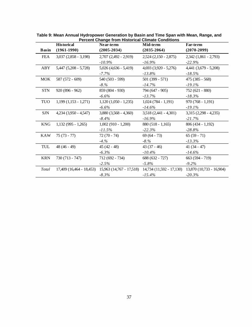
37

Table 9: Mean Annual Hydropower Generation by Basin and Time Span with Mean, Range, and Percent Change from Historical Climate Conditions

BasinHistorical(1961-1990)

Near-term(2005-2034)

Mid-term(2035-2064)

Far-term(2070-2099)

FEA 3,037 (2,858 - 3,198) 2,707 (2,492 - 2,919) 2,524 (2,150 - 2,875) 2,342 (1,861 - 2,793)-10.9% -16.9% -22.9%

ABY 5,447 (5,208 - 5,728) 5,026 (4,636 - 5,419) 4,693 (3,920 - 5,276) 4,441 (3,679 - 5,208)-7.7% -13.8% -18.5%

MOK 587 (572 - 609) 540 (503 - 599) 501 (399 - 571) 475 (385 - 568)-8.% -14.7% -19.1%

STN 920 (896 - 962) 859 (804 - 930) 794 (647 - 905) 752 (621 - 880)-6.6% -13.7% -18.3%

TUO 1,199 (1,153 - 1,271) 1,120 (1,050 - 1,235) 1,024 (784 - 1,191) 970 (768 - 1,191)-6.6% -14.6% -19.1%

SJN 4,234 (3,950 - 4,547) 3,880 (3,568 - 4,360) 3,518 (2,441 - 4,301) 3,315 (2,298 - 4,235)-8.4% -16.9% -21.7%

KNG 1,132 (995 - 1,265) 1,002 (910 - 1,200) 880 (518 - 1,165) 806 (434 - 1,192)-11.5% -22.3% -28.8%

KAW 75 (73 - 77) 72 (70 - 74) 69 (64 - 73) 65 (59 - 71)-4.% -8.% -13.3%

TUL 48 (46 - 49) 45 (42 - 48) 43 (37 - 46) 41 (34 - 47)-6.3% -10.4% -14.6%

KRN 730 (713 - 747) 712 (692 - 734) 688 (632 - 727) 663 (594 - 719)-2.5% -5.8% -9.2%

Total 17,409 (16,464 - 18,453) 15,963 (14,767 - 17,518) 14,734 (11,592 - 17,130) 13,870 (10,733 - 16,904)-8.3% -15.4% -20.3%

38

Section 7: Limitations

Spatiotemporal scope – As with all models, the SIERRA model is a simplified representation of real systems. The spatiotemporal scope of the model—weekly time step operations for most major reservoirs, hydropower plants, diversions, and instream flow requirement locations—necessitates analyses across watersheds and at the seasonal and annual time steps. Many small dams and diversions are omitted from the model for simplification, such as forebays, afterbays, and small water users that divert, store, and use water; these are currently unaccounted for. The spatiotemporal scope also affects included operations, since some hydropower generation decisions are made at the daily, hourly or shorter time step. This would affect simulation accuracy even with improved weekly-scale hydropower operations logic.

Inflow hydrology – The hydrologic model accuracy is a major limitation of the model, as applied. Because the hydrologic model used (Young et al. 2009) was calibrated only to the watershed outlets and to snow water equivalent at only 15 locations, inflow hydrology is under-represented in some locations and over-represented in other locations. This affects hydropower operations that depend on accurate inflows in specific locations rather than only at the watershed outlets.

Climate warming scenarios – Another important limitation of the inflow hydrology used for climate warming scenarios (Young et al. 2009) is the use of uniform and homogeneous changes in air temperature instead of location- and time-specific changes. Additionally, historical precipitation is assumed. Because some downscaled GCMs predict increased precipitation, while others predict less, it is important to assess impacts of warm-dry and warm-wet scenarios, as done by others (e.g., Madani and Lund 2010; Vicuna et al. 2008).

Climate warming effects – In the SIERRA model, warming only affects physical hydrology and lake evaporation. However, climate warming will also affect other important parameters that hydrology and water management decisions depend on. For example, atmospheric warming will likely increase energy demand; this effect is not represented in the model.

Hydropower generation – Hydropower operations here operate to a rule, whereas most hydropower systems operate for profit, responding to energy prices. The Water Year Index method works well in the long term, but does not account for weekly scale fluctuations in hydropower operations from hydropeaking or week-to-week price variability due to weather patterns. An optimization method is needed to more accurately simulate operations of hydropeaking facilities. One option is to assume the distribution of energy prices is known during the hydropeaking period, such that the optimal operation policy is to release during every hour that the energy price is above a threshold. A second option worth exploring is to establish relationships between power generation and watershed characteristics other than streamflow. For example, in California energy demand during the summer correlates with air temperature, since air conditioners, turned on when air temperature is high, are a major energy consumer.

Flood control and rim dams –Operation of rim dams, which were outside the spatial domain of the model, can affect upstream operations. For example, the Hetch Hetchy system is operated partially in coordination with flood control operations at New Don Pedro reservoir.

39

Inclusion of rim dams and upstream flood control operations would enable a better understanding of flood risk and control, including the possibility of utilizing higher reservoirs for some flood control.

Water supply demands – Existing water supply demand is limited in two ways. First, included demands are based on historical observations or known supply requirements. Water management projections should also include anticipated changes in other factors that affect future water demand such as future population growth and water use patterns in different sectors. Second, many smaller abstractions within the spatial extent of the model have been excluded for simplification. Including more of the smaller water diversions would help improve overall model accuracy.

Uncertainty and sensitivity – We did not conduct an uncertainty or sensitivity analysis for this model. Although there are several theoretically robust methods to help map uncertainty in inputs to uncertainty in outputs, the methods require substantial amounts of computational power. An analysis of the most obvious sources of uncertainty, such as inflow hydrology, and an assessment of which parameters the model is most sensitive to would be beneficial.

40

Section 8: Conclusions

The model presented here (SIERRA) is one of the larger hydropower and montane water resources simulation models. The main contribution of this work is both the model itself, including the methods for simulating hydropower generation, albeit coarse, and the quantitative assessment of hydropower generation impacts of regional climate warming. SIERRA can be used to assess effects of regional climate warming on a wide range of managed water systems and beneficial uses of water in the Sierra Nevada. The model performs well for hydropower facilities in the region for assessments of change at the seasonal and annual time scales.

Though other studies estimate climate change effects on hydropower, they are either very broad or very specific. The work here bridges the gap between generalized, state-wide studies and specific, local studies. We applied SIERRA at the weekly scale using climate warming scenarios of +0°C, 2°C, 4°C, and 6°C warming. Hydropower generation decreases in all warming scenarios, driven primarily by decreases in the highly productive watersheds in the northern Sierra Nevada. With far-term warming (+6°C), model results suggest about an 8 percent decrease in mean annual hydropower generation within the study region. This is less than estimates from other studies that consider drier conditions (less precipitation and runoff), but greater than studies that consider warming only (no change in annual runoff). Results from a Variable Infiltration Capacity hydrologic model using climate data from five GCMs are also included. Decreases in hydropower generation are much greater with GCM climate data and VIC hydrology than with WEAP hydrology, which does not consider changes in precipitation.

The most substantial decreases in mean annual hydropower generation occur in the northern watersheds, which have large decreases in runoff magnitude. In contrast, the model generally predicts a slight increase in generation with near- and mid-term warming followed by a slight decrease in generation with far-term warming. The model predicts constant declines in hydropower generation in the southern watersheds, though total generation in southern watersheds is small. These results suggest that future struggles over water use will be relatively more pronounced in the northern watersheds.

41

References

CDEC (California Data Exchange Center). (2010). "California Water Year Type Definitions."

Aspen Environmental Group, and M Cubed. (2005). "Potential Changes in Hydropower Production from Global Climate Change in California and the Western United States." California Energy Commission, Sacramento.

Bates, B. C., Kundzewicz, Z. W., Wu, S., and Palutikof, J. P. (2008). "Climate Change and Water. Technical Paper of the Intergovernmental Panel on Climate Change." IPCC Secretariat, Geneva.

Bower, B. T., Hufschmidt, M. M., and Reedy, W. W. (1966). "Operating Procedures: Their Role in the Design of Water-Resource Systems by Simulation Analysis." Design of Water-Resource Systems: New Techniques for Relating Economic Objectives, Engineering Analysis, and Governmental Planning, A. Maass, M. M. Hufschmidt, R. Dorfman, H. A. Thomas Jr., S. A. Marglin, and G. Maskew Fair, eds., Harvard University Press, Cambridge, Mass.

California Natural Resources Agency. (2009). "2009 California Climate Adaptation Strategy."

Dettinger, M. D., Cayan, D. R., Meyer, M., and Jeton, A. E. (2004). "Simulated hydrologic responses to climate variations and change in the Merced, Carson, and American River basins, Sierra Nevada, California, 1900-2099." Climatic Change 62(1-3), 283–317.

Dingman, S. L. (2002). Physical Hydrology. Prentice Hall, Upper Saddle River, New Jersey.

Draper, A., and Darabzand, S. (2003). "CalSim II Simulation of Historical SWP-CVP Operations." California Department of Water Resources.

Franco, G., and Sanstad, A. H. (2008). "Climate Change and Electricity Demand in California." Climatic Change 87(Suppl. 1), S139–S151.

Hayhoe, K., Cayan, D., Field, C. B., Frumhoff, P. C., Maurer, E. P., Miller, N. L., Moser, S. C., Schneider, S. H., Cahill, K. N., Cleland, E. E., Dale, L., Drapek, R., Hanemann, R. M., Kalkstein, L. S., Lenihan, J., Lunch, C. K., Neilson, R. P., Sheridan, S. C., and Verville, J. H. (2004). "Emissions pathways, climate change, and impacts on California." Proceedings of the National Academy of Sciences of the United States of America 101(34), 12422–12427.

Hickey, J. T., Bond, M. V., Patton, T. K., Richardson, K. A., and Pugner, P. E. (2003). "Reservoir Simulations of Synthetic Rain Floods for the Sacramento and San Joaquin River Basins." Journal of Water Resources Planning and Management 129, 443–457.

Jacobs, J., Freeman, G., Grygier, J., Morton, D., Schultz, G., Staschus, K., and Stedinger, J. (1995). "SOCRATES: A system for scheduling hydroelectric generation under uncertainty." Annals of Operations Research 59(1), 99–133.

Jain, S. K., and Sudheer, K. P. (2008). "Fitting of Hydrologic Models: A Close Look at the Nash-Sutcliffe Index." Journal of Hydrologic Engineering 13(10), 981–986.

42

Madani, K., and Lund, J. R. (2009). "Modeling California's high-elevation hydropower systems in energy units." Water Resources Research 45, W09413.

Madani, K., and Lund, J. R. (2010). "Estimated impacts of climate warming on California’s high-elevation hydropower." Climatic Change 102(3-4), 521–538.

Maurer, E. P., Wood, A. W., Adam, J. C., Lettenmaier, D. P., and Nijssen, B. (2002). "A Long-Term Hydrologically Based Dataset of Land Surface Fluxes and States for the Conterminous United States." Journal of Climate 15(22), 3237–3251.

Medellín-Azuara, J., Harou, J., Olivares, M., Madani, K., Lund, J., Howitt, R., Tanaka, S., Jenkins, M., and Zhu, T. (2008). "Adaptability and adaptations of California’s water supply system to dry climate warming." Climatic Change 87(0), 75–90.

Mehta, V. K., Rheinheimer, D. E., Yates, D., Purkey, D. R., Viers, J. H., Young, C. A., and Mount, J. F. (2011). "Potential impacts on hydrology and hydropower under climate warming of the Sierra Nevada." Journal of Water and Climate Change 2(1), 29–43.

Nash, J. E., and Sutcliffe, J. V. (1980). "River flow forecasting through conceptual models part I - A discussion of principles." Journal of Hydrology 10(3), 282–290.

Null, S. E., Viers, J. H., and Mount, J. F. (2010). "Hydrologic response and watershed sensitivity to climate warming in California's Sierra Nevada." PLoS ONE 5(4).

O'Brien, K. L., Eriksen, S., Nygaard, L. P., and Schjolden, A. (2007). "Why different interpretations of vulnerability matter in climate change discourses." Climate Policy 7(1), 73–88.

Rheinheimer, D. E., Ligare, S. T., and Viers, J. H. (2011). "A comparison of modeled Sierra Nevada discharge and meteorological data for hydrological vulnerability parameterization." University of California, Davis.

Tanaka, S. K., Zhu, T. J., Lund, J. R., Howitt, R. E., Jenkins, M. W., Pulido, M. A., Tauber, M., Ritzema, R. S., and Ferreira, I. C. (2006). "Climate Warming and Water Management Adaptation for California." Climatic Change 76(3-4), 361–387.

U.S. Army Corps of Engineers (USACE). (1998). "HEC-5: Simulation of flood control and conservation systems." Hydrologic Engineering Center, Davis, Calif.

Vicuña, S., Dracup, J. A., and Dale, L. (2009). "Climate change impacts on the operation of two high-elevation hydropower systems in California." California Climate Change Center.

Vicuña, S., Leonardson, R., Hanemann, M. W., Dale, L. L., and Dracup, J. A. (2008). "Climate change impacts on high elevation hydropower generation in California’s Sierra Nevada: A case study in the Upper American River." Climatic Change 87, 123–137.

Vicuña, S., Maurer, E. P., Joyce, B., Dracup, J. A., and Purkey, D. (2007). "The Sensitivity of California Water Resources to Climate Change Scenarios." Journal of the American Water Resources Association 43(2).

43

Yates, D., Sieber, J., Purkey, D., and Huber-Lee, A. (2005). "WEAP21 – A Demand-, Priority-, and Preference-Driven Water Planning Model: Part 1, Model Characteristics." Water International, 30(4), 487-500.

Young, C. A., Escobar-Arias, M. I., Fernandes, M., Joyce, B., Kiparsky, M., Mount, J. F., Mehta, V. K., Purkey, D., Viers, J. H., and Yates, D. (2009). "Modeling the Hydrology of Climate Change in California's Sierra Nevada for Subwatershed Scale Adaptation." Journal of the American Water Resources Association, 45(6), 1409-1423.

Glossary ABY American, Bear and Yuba Rivers

AMJ April, May, June

AMR American/Cosumnes River watersheds

CABY Cosumnes, American, Bear, and Yuba River watersheds

CAL Calaveras River watersheds

CDEC California Data Exchange Center

DEM digital elevation models

DWR California Department of Water Resources

EBHOM Energy-Based Hydropower Optimization Method

FEA Feather River watersheds

FERC Federal Energy Regulatory Commission

FNF full natural flow

GCM global circulation model

IFR instream flow requirement

JAS July, August, September

JFM January, February, March

KAW Kaweah River watersheds

KNG Kings River watersheds

KRN Kern River watersheds

MAF million acre-feet

44

MER Merced River watersheds

MIF minimum instream flow

MOK Mokelumne River watersheds

NLCD National Land Use Classification Database

NRCS Natural Resource Conservation Service

NSME Nash-Sutcliffe model efficiency

OND October, November, December

PG&E Pacific Gas & Electric Company

RMSE root mean square error

SDM spill demand method

SFPUC San Francisco Public Utilities Commission

SIERRA Sierra Integrated Environmental and Regulated Rivers Assessment

SJN San Joaquin River watersheds

STN Stanislaus River watersheds

SWE snow water equivalent

TUL Tule River watersheds

TUO Tuolumne River watersheds

UARP Upper American River Project

USACE U.S. Army Corps of Engineers

USGS U.S. Geological Survey

VIC variable infiltration capacity

WEAP Water Evaluation and Planning

WYI water year index

WYIM water year index method

WYT water year type

YUB Yuba/Bear River watersheds

45

Appendix A: SIERRA Input Parameters This Appendix includes the main physical and operations parameters used in SIERRA, including for reservoirs, run-of-river hydropower, variable head hydropower, water supply demand, instream flow requirements, and diversion conveyances. Some inconsistencies and conventions are worth noting. Source data units are usually in English units. However, WEAP uses SI units. In these tables, English units are mostly used, though some data are given in SI units.

Abbreviations and non-SI units in the tables are:

mcm = million cubic meters (1.0×106 m3) 1 AF = 1 acre-foot = 1.233×103 m3 1 ft = 1 foot = 3.048×10-1 m 1 ft3/s = 2.832×102m3/s

Other abbreviations include:

CDEC = California Data Exchange Center USGS = U.S. Geological Survey

Finally, we note again that the watersheds were grouped into mutually independent models (the latter are referred to in the main text), in order from north to south, as follows:

Watershed Model abbr. Watershed Model abbr.

Feather FEA Tuolumne TUO

Yuba

ABY

Merced MER

Bear San Joaquin SJN

American Kings KNG

Cosumnes Kaweah KAW

Mokelumne MOK Tule TUL

Calaveras CAL Kern KRN

Stanislaus STN

46

Table A-1. Reservoir Parameters

Watershed Name

Storage capacity (AF)

Storage capacity (mcm)

Minimum storage (mcm)

Min elevation (m)

Max. elevation (m)

Refill priority

Drawdown priority CDEC gauge USGS gauge

American

Caples Lake 21.6 26.6 2.5 0.0 100.0 15 15 CPL N/A

Chili Bar Reservoir 3.1 3.9 0 0.0 18.3 55 55 N/A N/A

French Meadows Reservoir 136.4 168.2 61.7 0.0 100.0 15 15 FMD N/A

Hell Hole Reservoir 207.3 255.7 38.8 / 86.3 1306.0 1417.3 25 25 HHL N/A

Ice House Reservoir 46.0 56.7 17.3 – 53.6 1623.8 1670.3 15 15 ICH 11441100

Loon Lake 76.5 94.3 0 1928.0 1959.9 15 15 LON 11429350

Oxbow Reservoir 24.3 30.0 0 0.0 75.0 45 45 N/A N/A

Rubicon Reservoir 1.5 1.8 0 1981.2 1996.4 15 15 N/A N/A

Silver Lake 8.6 10.7 0.5 0.0 50.0 15 15 SIV N/A

Slab Creek Reservoir 16.6 20.5 12.3 512.1 570.0 45 45 SLB 11443450

Stumpy Meadows Reservoir 20.0 24.7 0 0.0 100.0 45 45 EDN N/A

Union Valley Reservoir 277.0 341.5 3.0 1400.0 1484.4 25 25 UNV 11441001

Cosumnes Jenkinson Lake 41.0 50.6 0 0.0 50.0 65 65 JNK N/A

Feather

Antelope Lake 24.3 30.0 17 1497.2 1526.2 39 39 ANT N/A

Belden Reservoir 2.4 3.0 3.0 0.0 3.9 1 1 N/A N/A

Bucks Lake 105.6 130.2 80 1506.9 1571.2 16 16 BCL 11403500

Butt Valley Reservoir 49.9 61.5 36 1241.8 1259.5 15 15 BTV 11401050

Frenchman Lake 58.8 72.5 10.6 1669.7 1703.9 98 98 FRD N/A

Lake Almanor 1175.0 1448.8 750 1336.5 1370.2 15 15 ALM 11399000

Lake Davis 85.5 105.5 34.6 1728.2 1760.3 98 98 DAV N/A

Little Grass Valley Reservoir 89.8 110.7 55 1475.8 1538.3 15 15 LGV 11395020

47

Mountain Meadows Reservoir

24.8 30.6 0 1525.2 1533.1 15 15 MMW N/A

Sly Creek Reservoir 64.3 79.3 1.8 1004.3 1076.2 15 15 SLC 11395400

Kern Lake Isabella 562.4 693.4 0 746.5 794.0 15 15 ISB 11190500

Kings Courtright Reservoir 123.3 152.0 39 2400.9 2494.5 15 15 CTG 11214550

Wishon Reservoir 128.6 158.6 20 1917.1 1996.4 16 16 WSN 11214800

Mokelumne Lower Bear River Reservoir 52.0 64.1 4.1 1706.9 1773.9 16 16 LWB 11315600

Salt Springs Reservoir 141.9 174.9 6.2 1107.9 1206.4 29 29 SLS 11313500

San Joaquin

Bass Lake 45.1 55.6 27 986.3 1029.1 17 17 CNV 11243400

Florence Lake 64.4 79.4 1.25 2188.5 2233.4 15 99 FLR 11229600

Huntington Lake 89.2 109.9 37 2068.4 2118.4 15 15 HNT 11236000

Kerckhoff Lake 4.2 5.2 4.3 270.8 299.5 65 65 KRH 11246650

Lake Thomas A Edison 125.0 154.2 8 2281.0 2329.4 15 16 TAE 11231000

Mammoth Pool Reservoir 119.9 147.9 5 944.9 1015.0 26 26 MPL 11234700

Redinger Lake 26.1 32.2 5.28 359.8 427.6 55 55 RDN 11241950

Shaver Lake 135.6 167.2 0.47 1582.2 1636.8 25 25 SHV 11239500

Stanislaus

Beardsley Reservoir 98.5 121.5 25 953.1 1035.7 25 25 BRD 11292800

Donnells Reservoir 64.7 79.8 6.2 1411.5 1498.7 15 15 DON 11292600

Lyons Reservoir 4.9 6.0 1.25 1248.1 1286.3 26 26 LYS 11297700

New Spicer Meadow Reservoir

184.3 227.2 50 1940.1 2015.9 15 15 SPM 11293770

Pinecrest Reservoir 18.3 22.6 4 1671.2 1712.2 15 99 SWB 11297700

Relief Reservoir 12.3 15.2 1.2 2156.6 2232.1 15 15 RLF 11291000

Tuolumne Cherry Lake 274.3 338.2 0 1353.3 1433.5 17 17 CHY 11277200

Hetch Hetchy Reservoir 360.4 444.4 123.3 1070.5 1160.1 18 18 HTH 11275500

48

Lake Eleanor 26.1 32.2 0 1404.5 1421.3 15 17 ENR 11277500

Yuba-Bear

Bowman Lake 68.5 84.5 0 1648.9 1696.3 15 15 BWN 11415500

Buck Island Reservoir 1.1 1.3 0 1949.5 1964.7 15 15 N/A N/A

Camp Far West Lake 104.5 128.8 0 48.8 96.0 65 65 CFW N/A

Englebright Lake 70.0 86.3 74.0 0.0 85.3 35 35 ENG 11417950

Fordyce Lake 49.9 61.5 0.15 1914.1 1953.8 15 15 N/A 11414090

Jackson Meadows Reservoir 69.2 85.3 0 1794.2 1841.0 15 15 JCK 11407800

Lake Combie 5.6 6.8 0 0.0 26.0 55 55 CMB N/A

Lake Spaulding 75.1 92.6 0 1472.9 1540.8 15 15 SPG 11414140

New Bullards Bar Reservoir 966.1 1191.2 288.6 411.5 615.7 25 25 BUL 11413515

Rock Creek Reservoir 0.4 0.5 0 433.2 440.3 25 25 N/A N/A

Rollins Reservoir 66.0 81.4 0 596.0 662.3 45 45 RLL 11421800

Scotts Flat Reservoir 48.5 59.8 0 0.0 53.3 15 15 SFL 11418250

49

Table A-2. Fixed Head Hydropower Plant Parameters

Watershed Name Demand method

Max. flow (ft3/s)

Fixed head (ft)

Plant efficiency (%)

Hydropower priority

Spill demand priority Flow gauge EIA ID

American

Camino WYI 2000 997 90 39 39 USGS_11441895 430

El Dorado ID WYI 150 984 90 15 19 USGS_11439300 238

French Meadows WYI 400 656 90 15 19 USGS_11427200 424

Jaybird WYI 1378 1476 90 25 29 USGS_11441780 431

Jones Fork WYI 281 577 90 15 19 USGS_11440900 534

Loon Lake WYI 997 1100 90 15 19 USGS_11429340 432

Middle Fork WYI 920 1936 90 25 29 USGS_11428600 425

Ralston WYI 924 1312 90 39 39 USGS_11427765 427

Robbs Peak WYI 1046 330 90 25 25 USGS_11429300 433

White Rock WYI 3500 780 90 45 49 USGS_11443460 435

Feather

Belden Max Capacity 2410 770 90 N/A 25 USGS_11403050 219

Bucks Creek WYI 384 2558 90 15 19 USGS_11403700 220

Butt Valley Max Capacity 2118 362 90 N/A 29 USGS_11400600 221

Caribou 1 WYI 1114 1150 90 14 19 USGS_11401110 222

Caribou 2 WYI 1464 1151 90 14 19 USGS_11401110 223

Cresta Max Capacity 3510 290 90 N/A 49 USGS_11404360 231

Forbestown Max Capacity 620 795 90 N/A 25 USGS_11396290 417

Grizzly Max Capacity 375 705 90 N/A 29 USGS_11404240 7338

Hamilton Branch Max Capacity 200 410 90 N/A 21 N/A 242

Kanaka Max Capacity 32 542 90 N/A 15 USGS_11396396 54653

Kelly Ridge Max Capacity 255 628 90 N/A 35 USGS_11396329 418

50

Lime Saddle Max Capacity 87 462 90 N/A 29 N/A 255

Poe Max Capacity 3700 488 90 N/A 59 USGS_11404900 272

Rock Creek Max Capacity 2880 535 90 N/A 39 USGS_11403800 275

Toadtown Max Capacity 125 131 90 N/A 19 USGS_11389800 714

Woodleaf WYI 580 1456 90 14 25 USGS_11396090 419

Kaweah

Kaweah 1 Max Capacity 23 1260 90 N/A 19 USGS_11208720 337

Kaweah 2 Max Capacity 87 344 90 N/A 29 USGS_11208570 336

Kaweah 3 Max Capacity 97 750 90 N/A 19 USGS_11207500 338

Kern

Borel Max Capacity 590 255 90 N/A 14 USGS_11187500 328

Kern Canyon Max Capacity 705 264 90 N/A 49 USGS_11192940 7911

Kern River 1 Max Capacity 412 865 90 N/A 39 USGS_11192000 340

Kern River 3 Max Capacity 620 850 90 N/A 18 USGS_11185500 339

Rio Bravo Max Capacity 1500 121 90 N/A 59 USGS_11193010 50037

Kings

Balch 1 and 2 Max Capacity 843 2379 90 N/A 39 USGS_11216300 217 & 218

Haas WYI 825 2444 90 15 29 USGS_11216050 240

Helms Max Capacity 9000 1744 90 N/A 19 USGS_11214540 6100

Kings River Max Capacity 990 798 90 N/A 49 USGS_11218700 254

Mokelumne

Electra Max Capacity 1130 1272 90 N/A 49 PG&E_M65 239

Salt Springs 2 WYI 225 2117 90 15 19 USGS_11313510 N/A

Tiger Creek WYI 750 1219 90 25 29 USGS_11316610 287

West Point Max Capacity 675 312 90 N/A 39 PG&E_M64 291

San Joaquin

Big Creek 1 WYI 692 1923 90 14 18 USGS_11238100 317

Big Creek 2 Max Capacity 607 1638 90 N/A 29 USGS_11238380 318

Big Creek 2A WYI 625 2200 90 25 19 USGS_11238400 322

51

Big Creek 3 Max Capacity 3200 764 90 N/A 49 USGS_11241800 319

Big Creek 4 WYI 3700 388 90 55 59 USGS_11246530 320

Big Creek 8 Max Capacity 1332 685 90 N/A 39 USGS_11238550 321

Eastwood WYI 2296 1312 90 15 19 USGS_11238250 104

Kerckhoff 1 WYI 1735 351 90 64 69 USGS_11246950 250

Kerckhoff 2 WYI 5100 420 90 65 69 USGS_11247050 682

Mammoth Pool WYI 2500 1004 90 25 29 USGS_11235100 344

Portal Max Capacity 724 190 90 N/A 29 USGS_11235500 354

San Joaquin 1 Max Capacity 235 1305 90 N/A 49 USGS_11246610 293

San Joaquin 1A Max Capacity 167 40 90 N/A 39 USGS_11246590 278

San Joaquin 2 Max Capacity 150 292 90 N/A 29 USGS_11246570 276

San Joaquin 3 WYI 150 378 90 15 19 USGS_11244100 277

Stanislaus

Angels Max Capacity 40 444 90 N/A 39 N/A 215

Collierville WYI 1400 2192 90 15 19 USGS_11295250 54555

Donnells WYI 700 1151 90 19 19 USGS_11292610 415

Murphys Max Capacity 68 684 90 N/A 29 N/A 261

Phoenix WYI 25 25 90 25 29 PG&E_S108 264

Sand Bar WYI 600 427 90 25 29 USGS_11292860 777

Spring Gap WYI 59 1865 90 15 39 USGS_11297000 284

Stanislaus WYI 830 1520 90 25 39 USGS_11295505 285

Tule Lower Tule R Max Capacity 35 1140 90 N/A 29 USGS_11202700 365

Tule River Max Capacity 70 1544 90 N/A 19 USGS_11201700 289

Tuolumne Dion R Holm WYI 1000 2100 90 15 19 SFPUC_HPH 380

Kirkwood WYI 1400 1100 90 15 19 SFPUC_KPH 382

52

Moccasin WYI 1200 1240 90 16 29 SFPUC_MPH 381

Yuba-Bear

Alta Max Capacity 56 650 90 N/A 20 USGS_11421725 214

Chicago Park WYI 1100 480 90 39 39 USGS_11421780 412

Colgate WYI 3400 1306 90 25 29 USGS_11413510 454

Deer Creek WYI 66 838 90 14

USGS_11414205 233

Drum 1 WYI 360 1379 90 15 19 USGS_11414194 235

Drum 2 WYI 500 1376 90 15 19 USGS_11414195 236

Dutch Flat 1 WYI 490 581 90 15 29 USGS_11421750 237

Dutch Flat 2 WYI 600 581 90 15 29 USGS_11421760 413

Halsey WYI 294 326 90 48 48 USGS_11425310 241

Narrows 1 WYI 730 236 90 35 39 USGS_11417970 262

Narrows 2 WYI 3400 200 90 35 39 USGS_11417980 455

Newcastle WYI 392 410 90 59 59 USGS_11425416 632

Spaulding 1 WYI 550 198 90 19 19 USGS_11414154 281

Spaulding 2 WYI 200 346 90 18 18 USGS_11414155 282

Spaulding 3 WYI 330 328 90 17 17 USGS_11416200 283

Wise 1 and 2 WYI 473 522 90 59 59 USGS_11425415 292

53

Table A-3. Variable Head Hydropower Plant Parameters

Watershed Name Owner Reservoir Max. flow

(ft3/s) Efficiency

(%) Tailwater

elevation (m) Flow gauge EIA ID

American

Chili Bar Pacific Gas & Electric Co Chili Bar Reservoir 1659 90 0.0 N/A 225

Hell Hole Placer County Water Agency Hell Hole Reservoir 20 90 1306.0 N/A 763

Oxbow Placer County Water Agency Oxbow Reservoir 1100 90 0.0 USGS_11433212 426

Slab Creek Sacramento Municipal Utility Dist. Slab Creek Reservoir 36 90 515.1 N/A 522

Union Valley Sacramento Municipal Utility Dist. Union Valley Reservoir 1577 90 1400.0 USGS_11441002 6612

Feather Oak Flat Pacific Gas & Electric Co Belden Reservoir 140 90 0.0 N/A 626

Sly Creek Northern California Power Agency Sly Creek Reservoir 700 90 1104.3 USGS_11395400 776

Mokelumne Salt Springs 1 Pacific Gas & Electric Co Salt Springs Reservoir 225 90 1107.9 CDEC_SLS 279

San Joaquin Crane Valley Pacific Gas & Electric Co Bass Lake 160 90 986.3 USGS_11243400 230

Stanislaus

Beardsley Oakdale & South San Joaquin Irr. Dist.

Beardsley Reservoir 620 90 953.1 USGS_11292800 414

New Spicer Meadow

Northern California Power Agency New Spicer Meadow Reservoir

200 90 1940.1 USGS_11293760 54554

Yuba-Bear

Bowman Pacific Gas & Electric Co Bowman Lake 313 90 1647.7 N/A 848

Camp Far West Sacramento Municipal Utility Dist. Camp Far West Lake 25 90 48.8 N/A 531

Combie Nevada Irrigation District Lake Combie 5 90 0.0 N/A 846 & 847

Fish Power Yuba County Water Agency New Bullards Bar 5 90 411.5 N/A 4229

Rollins Nevada Irrigation District Rollins Reservoir 840 90 597.0 USGS_11421900 34

54

Table A-4. Water Supply Demand Parameters

Watershed Supply demand name Weekly demand Annual demand (million m3) Weekly variation Demand Priority

American Folsom N/A 10.7 Variable 65

Feather

California Water Service Company (CalWater) - Oroville N/A 38.5 Variable 23

South Feather Water & Power Agency (SFWPA) - Bangor N/A 11.4 Variable 25

South Feather Water & Power Agency (SFWPA) - Forbestown N/A 7.5 Variable 13

Mokelumne Amador Water Agency (AWA) N/A 1.7 Constant 33

Calaveras Public Utilities District (CPUD) N/A 1.9 Constant 13

Tule

Crabtree-Aiken Ditch Co. N/A 5.8 Constant 23

Graham Osborn Ditch Co. N/A 10.7 Constant 23

Mt Whitney Ditch Co. N/A 3.6 Constant 22

Pleasant Valley Canal Co. N/A 10.7 Constant 23

South Tule Ditch Co. N/A 14.3 Constant 13

Tuolumne San Francisco Public Utilities Commission (SFPUC) N/A (-0.0116*WYI_SJValley + 0.26)*1233 Variable 13

Yuba-Bear

Nevada Irrigation District (NID) 1 Variable N/A N/A 23

Nevada Irrigation District (NID) 2 Variable N/A N/A 23

Nevada Irrigation District (NID) 3 Variable N/A N/A 53

Nevada Irrigation District (NID) 4 Cascade Variable N/A N/A 13

Nevada Irrigation District (NID) 5 Deer Creek Variable N/A N/A 13

Placer County Water Agency (PCWA) 1 Variable N/A N/A 13

Placer County Water Agency (PCWA) 2 Variable N/A N/A 43

Placer County Water Agency (PCWA) 3 Variable N/A N/A 24

Placer County Water Agency (PCWA) 4 Variable N/A N/A 24

Placer County Water Agency (PCWA) 5 Variable N/A N/A 24

Sly Folsom N/A 9.3 Variable 65

South Fork Feather River (SFFR) N/A (0.003*WYI_SacValley + 0.0522)*1233 Variable 13

Yuba County Water Agency (YCWA) Wheatland Variable N/A N/A 47

55

Table A-5. Instream Flow Requirement (IFR) Parameters

Watershed Name River Regulator Definition source Priority

American

IFR bl Buck Island Little Rubicon Buck Island Reservoir P-2101 FERC license 12

IFR bl Buck Loon Tunnel Rubicon River Buck Look Diversion P-2101 FERC license 13

IFR blCaples CaplesCr. Caples Lake P-0184 FERC license 11

IFR bl Chili Bar S Fk American Chili Bar Reservoir P-2155 FERC license 51

IFR bl Duncan Tunnel Duncan Cr. Duncan Tunnel Div. Reservoir P-2079 FERC license 11

IFR bl El Dorado ID Canal S Fk American El Dorado ID Div. Reservior P-0184 FERC license 12

IFR bl French Meadows M Fork American French Meadows Reservoir P-2079 FERC license 12

IFR bl Hell Hole Rubicon River Hell Hole Reservoir P-2079 FERC license 21

IFR bl Ice House S Fk Silver Creek Ice House Reservoir P-2101 FERC license 11

IFR bl Jaybird Tunnel Silver Cr. Junction Reservoir P-2101 FERC license 22

IFR bl Long Canyon Creek Tunnel Long Canyon Cr. Long Canyon Creek Tunnel P-2079 FERC license 21

IFR bl Loon GerleCr. Loon Lake P-2101 FERC license 14

IFR bl Ralston Tunnel M Fork American Ralston Tunnel P-2079 FERC license 31

IFR bl Rubicon Rubicon River Rubicon Reservoir P-2101 FERC license 11

IFR bl Silver Silver Fk American Silver Lake P-0184 FERC license 11

IFR bl Slab Creek S Fk American Slab Cr. Reservoir P-2101 FERC license 41

Cosumnes IFR bl Camp Creek Tunnel Camp Cr. Camp Creek Tunnel Central Valley Project, Sly Park Unit 11

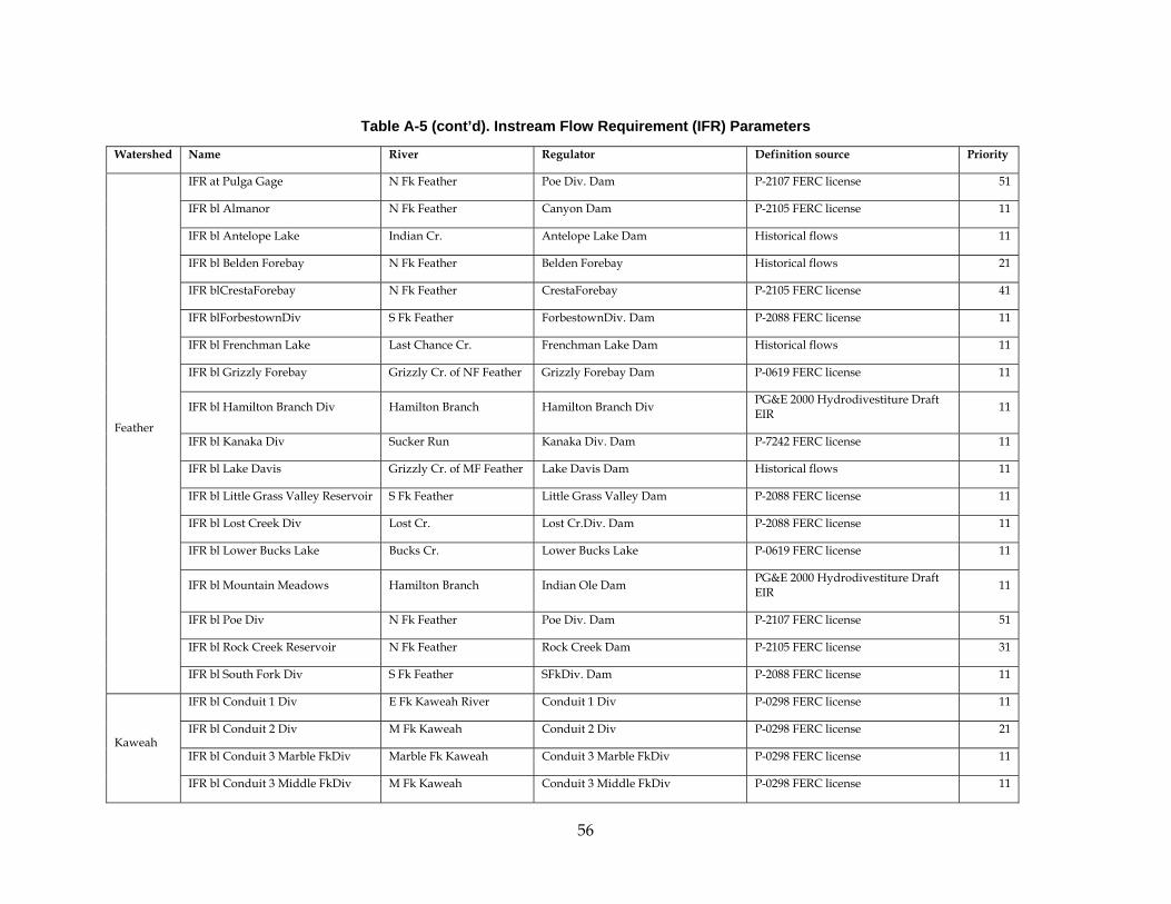
56

Table A-5 (cont’d). Instream Flow Requirement (IFR) Parameters

Watershed Name River Regulator Definition source Priority

Feather

IFR at Pulga Gage N Fk Feather Poe Div. Dam P-2107 FERC license 51

IFR bl Almanor N Fk Feather Canyon Dam P-2105 FERC license 11

IFR bl Antelope Lake Indian Cr. Antelope Lake Dam Historical flows 11

IFR bl Belden Forebay N Fk Feather Belden Forebay Historical flows 21

IFR blCrestaForebay N Fk Feather CrestaForebay P-2105 FERC license 41

IFR blForbestownDiv S Fk Feather ForbestownDiv. Dam P-2088 FERC license 11

IFR bl Frenchman Lake Last Chance Cr. Frenchman Lake Dam Historical flows 11

IFR bl Grizzly Forebay Grizzly Cr. of NF Feather Grizzly Forebay Dam P-0619 FERC license 11

IFR bl Hamilton Branch Div Hamilton Branch Hamilton Branch Div PG&E 2000 Hydrodivestiture Draft EIR

11

IFR bl Kanaka Div Sucker Run Kanaka Div. Dam P-7242 FERC license 11

IFR bl Lake Davis Grizzly Cr. of MF Feather Lake Davis Dam Historical flows 11

IFR bl Little Grass Valley Reservoir S Fk Feather Little Grass Valley Dam P-2088 FERC license 11

IFR bl Lost Creek Div Lost Cr. Lost Cr.Div. Dam P-2088 FERC license 11

IFR bl Lower Bucks Lake Bucks Cr. Lower Bucks Lake P-0619 FERC license 11

IFR bl Mountain Meadows Hamilton Branch Indian Ole Dam PG&E 2000 Hydrodivestiture Draft EIR

11

IFR bl Poe Div N Fk Feather Poe Div. Dam P-2107 FERC license 51

IFR bl Rock Creek Reservoir N Fk Feather Rock Creek Dam P-2105 FERC license 31

IFR bl South Fork Div S Fk Feather SFkDiv. Dam P-2088 FERC license 11

Kaweah

IFR bl Conduit 1 Div E Fk Kaweah River Conduit 1 Div P-0298 FERC license 11

IFR bl Conduit 2 Div M Fk Kaweah Conduit 2 Div P-0298 FERC license 21

IFR bl Conduit 3 Marble FkDiv Marble Fk Kaweah Conduit 3 Marble FkDiv P-0298 FERC license 11

IFR bl Conduit 3 Middle FkDiv M Fk Kaweah Conduit 3 Middle FkDiv P-0298 FERC license 11

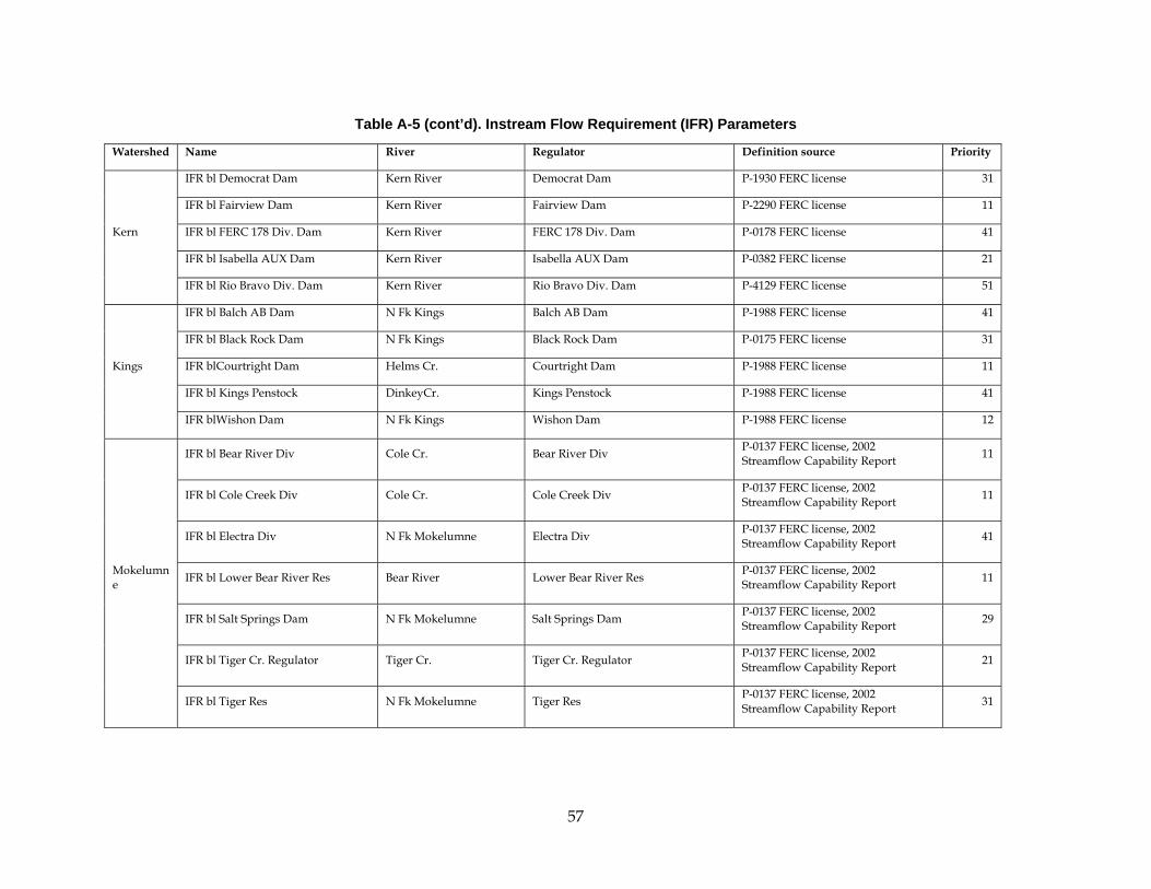
57

Table A-5 (cont’d). Instream Flow Requirement (IFR) Parameters

Watershed Name River Regulator Definition source Priority

Kern

IFR bl Democrat Dam Kern River Democrat Dam P-1930 FERC license 31

IFR bl Fairview Dam Kern River Fairview Dam P-2290 FERC license 11

IFR bl FERC 178 Div. Dam Kern River FERC 178 Div. Dam P-0178 FERC license 41

IFR bl Isabella AUX Dam Kern River Isabella AUX Dam P-0382 FERC license 21

IFR bl Rio Bravo Div. Dam Kern River Rio Bravo Div. Dam P-4129 FERC license 51

Kings

IFR bl Balch AB Dam N Fk Kings Balch AB Dam P-1988 FERC license 41

IFR bl Black Rock Dam N Fk Kings Black Rock Dam P-0175 FERC license 31

IFR blCourtright Dam Helms Cr. Courtright Dam P-1988 FERC license 11

IFR bl Kings Penstock DinkeyCr. Kings Penstock P-1988 FERC license 41

IFR blWishon Dam N Fk Kings Wishon Dam P-1988 FERC license 12

Mokelumne

IFR bl Bear River Div Cole Cr. Bear River Div P-0137 FERC license, 2002 Streamflow Capability Report

11

IFR bl Cole Creek Div Cole Cr. Cole Creek Div P-0137 FERC license, 2002 Streamflow Capability Report

11

IFR bl Electra Div N Fk Mokelumne Electra Div P-0137 FERC license, 2002 Streamflow Capability Report

41

IFR bl Lower Bear River Res Bear River Lower Bear River Res P-0137 FERC license, 2002 Streamflow Capability Report

11

IFR bl Salt Springs Dam N Fk Mokelumne Salt Springs Dam P-0137 FERC license, 2002 Streamflow Capability Report

29

IFR bl Tiger Cr. Regulator Tiger Cr. Tiger Cr. Regulator P-0137 FERC license, 2002 Streamflow Capability Report

21

IFR bl Tiger Res N Fk Mokelumne Tiger Res P-0137 FERC license, 2002 Streamflow Capability Report

31

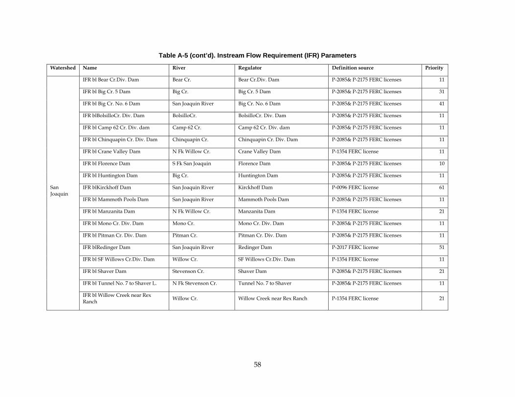
58

Table A-5 (cont’d). Instream Flow Requirement (IFR) Parameters

Watershed Name River Regulator Definition source Priority

San Joaquin

IFR bl Bear Cr.Div. Dam Bear Cr. Bear Cr.Div. Dam P-2085& P-2175 FERC licenses 11

IFR bl Big Cr. 5 Dam Big Cr. Big Cr. 5 Dam P-2085& P-2175 FERC licenses 31

IFR bl Big Cr. No. 6 Dam San Joaquin River Big Cr. No. 6 Dam P-2085& P-2175 FERC licenses 41

IFR blBolsilloCr. Div. Dam BolsilloCr. BolsilloCr. Div. Dam P-2085& P-2175 FERC licenses 11

IFR bl Camp 62 Cr. Div. dam Camp 62 Cr. Camp 62 Cr. Div. dam P-2085& P-2175 FERC licenses 11

IFR bl Chinquapin Cr. Div. Dam Chinquapin Cr. Chinquapin Cr. Div. Dam P-2085& P-2175 FERC licenses 11

IFR bl Crane Valley Dam N Fk Willow Cr. Crane Valley Dam P-1354 FERC license 11

IFR bl Florence Dam S Fk San Joaquin Florence Dam P-2085& P-2175 FERC licenses 10

IFR bl Huntington Dam Big Cr. Huntington Dam P-2085& P-2175 FERC licenses 11

IFR blKirckhoff Dam San Joaquin River Kirckhoff Dam P-0096 FERC license 61

IFR bl Mammoth Pools Dam San Joaquin River Mammoth Pools Dam P-2085& P-2175 FERC licenses 11

IFR bl Manzanita Dam N Fk Willow Cr. Manzanita Dam P-1354 FERC license 21

IFR bl Mono Cr. Div. Dam Mono Cr. Mono Cr. Div. Dam P-2085& P-2175 FERC licenses 11

IFR bl Pitman Cr. Div. Dam Pitman Cr. Pitman Cr. Div. Dam P-2085& P-2175 FERC licenses 11

IFR blRedinger Dam San Joaquin River Redinger Dam P-2017 FERC license 51

IFR bl SF Willows Cr.Div. Dam Willow Cr. SF Willows Cr.Div. Dam P-1354 FERC license 11

IFR bl Shaver Dam Stevenson Cr. Shaver Dam P-2085& P-2175 FERC licenses 21

IFR bl Tunnel No. 7 to Shaver L. N Fk Stevenson Cr. Tunnel No. 7 to Shaver P-2085& P-2175 FERC licenses 11

IFR bl Willow Creek near Rex Ranch

Willow Cr. Willow Creek near Rex Ranch P-1354 FERC license 21

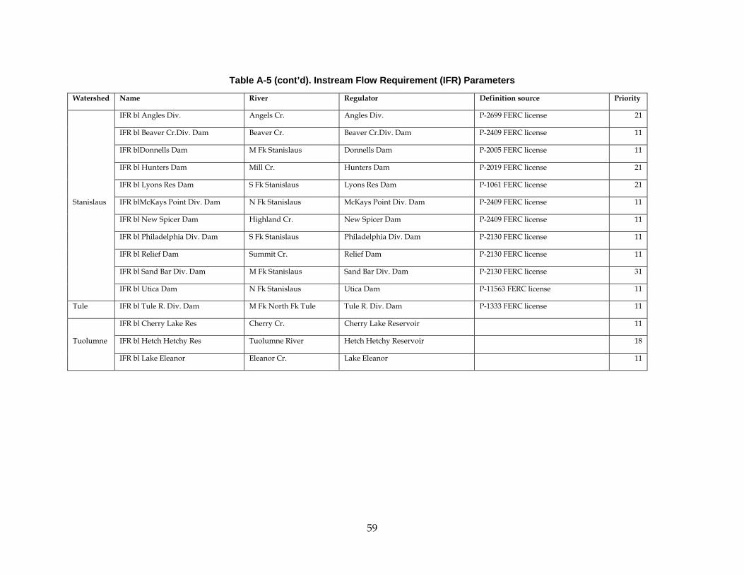
59

Table A-5 (cont’d). Instream Flow Requirement (IFR) Parameters

Watershed Name River Regulator Definition source Priority

Stanislaus

IFR bl Angles Div. Angels Cr. Angles Div. P-2699 FERC license 21

IFR bl Beaver Cr.Div. Dam Beaver Cr. Beaver Cr.Div. Dam P-2409 FERC license 11

IFR blDonnells Dam M Fk Stanislaus Donnells Dam P-2005 FERC license 11

IFR bl Hunters Dam Mill Cr. Hunters Dam P-2019 FERC license 21

IFR bl Lyons Res Dam S Fk Stanislaus Lyons Res Dam P-1061 FERC license 21

IFR blMcKays Point Div. Dam N Fk Stanislaus McKays Point Div. Dam P-2409 FERC license 11

IFR bl New Spicer Dam Highland Cr. New Spicer Dam P-2409 FERC license 11

IFR bl Philadelphia Div. Dam S Fk Stanislaus Philadelphia Div. Dam P-2130 FERC license 11

IFR bl Relief Dam Summit Cr. Relief Dam P-2130 FERC license 11

IFR bl Sand Bar Div. Dam M Fk Stanislaus Sand Bar Div. Dam P-2130 FERC license 31

IFR bl Utica Dam N Fk Stanislaus Utica Dam P-11563 FERC license 11

Tule IFR bl Tule R. Div. Dam M Fk North Fk Tule Tule R. Div. Dam P-1333 FERC license 11

Tuolumne

IFR bl Cherry Lake Res Cherry Cr. Cherry Lake Reservoir

11

IFR bl Hetch Hetchy Res Tuolumne River Hetch Hetchy Reservoir

18

IFR bl Lake Eleanor Eleanor Cr. Lake Eleanor

11

60

Table A-5 (cont’d). Instream Flow Requirement (IFR) Parameters

Watershed Name River Regulator Definition source Priority

Yuba-Bear

IFR bl Bear Meadow Bear R Bear Meadow P-2310 FERC license 11

IFR bl Bowman Canyon Cr. Bowman Lake P-2266 FERC license 12

IFR bl Camp Far West Bear R Camp Far West Reservoir

61

IFR blCombie Bear R Lake Combie P-2266 FERC license 51

IFR bl Daguerre Point Yuba River Daguerre Point Div. Reservoir State Water Resources Control Board RD-1644

46

IFR bl Drum Afterbay Bear River Drum Afterbay P-2310 FERC license 14

IFR bl Dutch Flat Afterbay Bear River Dutch Flat Afterbay P-2266 FERC license 31

IFR bl Fordyce Fordyce Cr. Lake Fordyce P-2310 FERC license 11

IFR bl Jackson Meadows M Fk Yuba Jackson Meadows Reservoir P-2266 FERC license 10

IFR bl Milton M Fk Yuba Milton Div. Reservoir P-2266 FERC license 11

IFR bl Narrows at Smartville Yuba River Englebright Reservoir State Water Resources Control Board RD-1644

31

IFR bl New Bullards Bar N Fk Yuba New Bullards Bar Reservoir P-2246 FERC license 23

IFR bl Oregon Creek Div Oregon Cr. Oregon Creek Div. P-2246 FERC license 22

IFR bl Our House M Fk Yuba Our House Div. Reservoir P-2246 FERC license 21

IFR bl Rollins Bear R Rollins Reservoir P-2266 FERC license 41

IFR bl Scotts Flat Deer Cr. Scotts Flat Reservoir

11

IFR bl South Canal Inflow Mormon Ravine South Canal Inflow P-2310 FERC license 51

IFR bl Spaulding at Langs Crossing S Fk Yuba Lake Spaulding P-2310 FERC license 12

IFR bl Spaulding at Spaulding 2 PH S Fk Yuba R bl Spaulding

Lake Spaulding P-2310 FERC license 11

61

Table A-6. Conveyance Parameters

Watershed Conveyance

Max. capacity (ft3/s) Watershed Conveyance

Max. capacity (ft3/s)

American

Buck Loon Tunnel 1260

Kings

Balch Tunnel 843

Camino Tunnel 2000 Haas Tunnel 825

Camp CreekTunnel 500 Helms Aqueduct 9000

Duncan Tunnel 400 Kings Aqueduct Dinkey Cr. Div.

10

El Dorado ID Canal 165 Kings River Aqueduct 950

French Meadows Hell Hole Tunnel

400

Mokelumne

Bear River Div. 85

Hell Hole Middle Fork Tunnel 920 Bear River Div. Tunnel, Fwd 800

Jaybird Tunnel 1345 Bear River Div. Tunnel, Rev 800

Jones Fork Tunnel 287 Cole Creek Div. N/A

Long Canyon Creek Tunnel 300 Electra Tunnel 875

Loon Lake Tunnel 997 Lower Tiger Cr. Div. Tunnel 625

Ophir Tunnel N/A Salt Springs 2 Penstock 225

Ralston Tunnel 836 Tiger Creek Canal 550

Robbs Peak Tunnel 1250 West Point Diversion 675

Rockbound Tunnel 1300

San Joaquin

Balsam Diversion Tunnel 2500

Sly Park Canal N/A Bear Diversion Tunnel 450

White Rock Tunnel 3500 Big Creek 3 Aqueduct 3250

Feather

Belden Tunnel 2410 Big Creek 4 Aqueduct 3700

Bucks Diversion 330 Big Creek 8 Penstock 1173

Butt Valley Tunnel 2118 Browns Creek Ditch 80

Caribou 1 Penstock 1114 Eastwood Tunnel 2500

Caribou 2 Penstock 1464 Kerckhoff 1 Tunnel 6500

Cresta Tunnel 3850 Kerckhoff 2 Tunnel 5100

Forbestown Diversion 660 Mammoth Pool Tunnel 2500

62

Grizzly Forebay Tunnel 360 Mono Tunnel 650

Grizzly Tunnel 400 No. 1 Conduit 210

Hamilton Branch 210 No. 2 Conduit 160

Hendricks Canal 125 No. 3 Conduit 160

Kanaka Div 37 PH 2A Aqueduct 650

Kelly Ridge Div 350 Portal Aqueduct 650

Miners Ranch Canal 300 Portal Penstock 1500

Poe Aqueduct 3700 Tunnel No. 1 700

Rock Creek Tunnel 2880 Tunnel No. 2 620

Slate Cr Tunnel 848 Tunnel No. 7 2439

South Fork Diversion Tunnel 600 Ward Tunnel 1760

Upper Miocene Canal 65

Stanislaus

Angels Canal 45

Woodleaf Diversion 620 DonnellsDiv 750

Kaweah

Conduit No. 3 97 Lower Collierville Tunnel 1 1475

Conduit No. 3 Marble Fk 50 Lower Collierville Tunnel 2 1475

Conduit No. 3 Middle Fk 65 Lower Utica Canal 45

Kaweah 1 Aqueduct 25 Phoenix Canal 33

Kaweah 2 Aqueduct 85 Philadelphia Aqueduct 60

Kern

Borel Canal 605 Sand Bar Power Tunnel 600

Kern Canyon Aqueduct 750 Stanislaus Tunnel 530

Kern River 3 Aqueduct 590 UPA Tunnel Tap 88

Kern River Flume 412 Upper Collierville Tunnel 200

Rio Bravo Canal 1800 Upper Utica Canal 88

63

A-6 (cont’d). Conveyance Parameters

Watershed Conveyance

Max. capacity (ft3/s)

Tule Lower Tule R Aqueduct 35

Upper Tule R Conduit 66

Tuolumne

Canyon Power Tunnel 1500

Dion R. Holm Tunnel 1000

Hetch Hetchy Aqueduct 900

Hetch Hetchy Aqueduct to SF 465

Lake Eleanor Tunnel 720

Moccasin Aqueduct 900

Yuba-Bear

Bear River Canal 470

Bowman Spaulding Conduit 325

Texas Creek Div. 250

Camptonville Tunnel 1071

Chicago Park Flume 1100

Drum 1 Penstock 360

Drum 2 Penstock 500

Drum Bear Div. N/A

Drum Canal 840

Dutch Flat 1 490

Dutch Flat 2 610

Lohman Ridge Tunnel 1071

Lower Boardman Canal N/A

Lower Wise Canal 473

64

Milton Bowman Tunnel 429

Narrows 1 Penstock 70

Narrows 2 Penstock 3490

New Colgate Tunnel 3800

South Canal 375

S. Canal to Mormon Ravine N/A

South Yuba Canal 125

Towle Canal 42

Upper Wise Canal 488