EMPLOYMENT, OUTPUT AND REAL WAGES

Bill Russell

and

Warren J. Tease

Research Discussion Paper 8806

September 1988

Research Department Reserve Bank of Australia

i

ABSTRACf

Employment in Australia over the past five years has recorded one of the strongest increases in the post-war period. This experience stands in marked contrast to that of the mid 1970s and early 1980s when demand for labour in Australia was very weak.

Recent developments provide an opportunity to look again at the relative importance of two main factors affecting the demand for labour - viz, output and real wages. This paper presents estimates of the relationship between employment, output and real wages over the past two decades. The study therefore covers three major episodes in the labour market: the contractions in employment in the mid 1970s and early 1980s and the strong growth since 1983.

The paper finds that real wages have been an important influence on employment in Australia- on average, just as important as output. The results show that a large part of the strength of employment over the past five years has been due to the fall in real wages.

ii

TABLE OF CONTENTS

Abstract

Table of Contents

1. Introduction

2. Trends in Employment, Output and Real Wages

(a) The 1974/75 Episode (b) The 1982/83 Episode (c) The Past Five Years

3. Employment, Output and Wages: The Evidence from Previous Studies

4. Employment Output and Real Wages Revisited

(a) The Specification

(b) Data and Results

5. Simulation Results

6. Conclusion

7. Bibliography

8. Appendices

i

ii

1

1

2 4 5

5

9

9

10

12

16

17

20

1

EMPLOYMENT, OUTPUT AND REAL WAGES

Bill Russell and Warren J. Tease

1. Introduction

Employment in Australia over the past five years has recorded one of the strongest increases in the post-war period. The performance ranked Australia first among the developed countries in terms of employment growth over the period. This experience stands in marked contrast with that of the mid 1970s and early 1980s when demand for labour in Australia was very weak.

Recent developments provide an opportunity to look again at the relative importance of two factors affecting the demand for labour- viz, output and real wages. This issue was the subject of considerable debate in the second half of the 1970s, both in Australia and overseas, and a large body of literature developed.

This paper presents estimates of the relationship between employment, output and real wages over the past two decades. The study therefore covers three major episodes in the labour market: the contractions of employment in the mid 1970s and early 1980s and the strong growth since 1983. It finds that real wages have been an important influence on employment in Australia- on average, just as important as output. A large part of the strength of employment over the past five years has been due to the fall in real wages.

Section 2 outlines the broad trends in employment, output and wages in the 1970s and 1980s. Section 3 reviews the Australian and some overseas literature on the relationship between these variables while Section 4 presents the results of the empirical work. Section 5 provides estimates of the contributions of real wages and output to employment growth in the three major episodes mentioned above. Some concluding thoughts are provided in Section 6.

2. Trends in Employment, Output and Real Wages

Over the 1970s and 1980s, employment has grown at an average rate of about 1.8 per cent per annum. Within the total, part-time employment has increased more quickly than full-time employment; the average annual growth rates of these two categories of employment have been 5.2 per cent

2

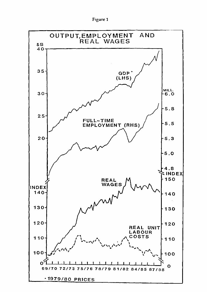
and 1.2 per cent respectively1. Output (as measured by real gross domestic product) increased by 3.4 per cent per annum over this period. Trends in gross domestic product and full-time employment over the 1970s and 1980s are shown in Figure 1. (The data are provided in Appendix 3.)

The faster growth of output compared with employment reflects the rise in productivity, or output per employed person. After allowing for changes in hours worked, due in part to the compositional shift between full-time and part-time employment, productivity has increased on average by 2.1 per cent per annum over the period.

Movements in real wages over the two decades are shown in the lower part of Figure 1. Over this period, real wages have risen at an average annual rate of about 2.1 per cent. This is the same as the growth of productivity.

With real payments to labour on average increasing in line with productivity, the real cost of labour per unit of output showed little net change over the period. This is shown in Figure 1 by the line representing real unit labour costs which adjusts the increase in real wages for the increase in productivity. The index of real unit labour costs at the end of the period was approximately 100, much the same as it had been at the start.

There have been periods, however, when the growth of wages has diverged markedly from productivity. There were three such episodes in the past two decades. In the mid 1970s and early 1980s, real unit labour costs rose sharply while over the past five years they have fallen. These episodes have coincided with large changes in employment growth. In 1974/75 and 1982/83, there were sharp falls in full-time employment, while there has been a prolonged rise in full-time employment since September 1983.

Each of these episodes is discussed in detail below.

(a) The 1974/75 Episode

After growing steadily in the early 1970s, total employment peaked in June 197 4 and then fell sharply over the next three quarters. From peak to trough, the fall was 78,000 or 1-1/4 per cent. Full-time employment fell more sharply over this period- by 137,000 or 2-1/2 per cent. The fall in employment in 1974/75 was, at the time, the largest since the 1930s.

The fall in employment was more than would have been expected given the behaviour of output. Output peaked in December 1973 and then fell by

1 To abstract from compositional shifts betwen full-time and part-time employment, this study focuses mainly on full-time employment.

$8

Figure 1

OUTPU~EMPLOYMENT REAL WAGES

AND

40-------------------------------------.

35

30

25

20

INDEX 140

130

120

GOP• (LHS)

FULL-TIME EMPLOYMENT

REAL WAGES

REAL UNIT LABOUR

5.8

4.8 INDEX 150

140

130

120

110 /'\ ,. .!\COSTS 110 I "'' ~.1' \ . I '

100

• "' ' I \ I \1' '' I'·'' \-I "' ~'

, ""'' ,. "' ,.,f\ I I \1 ' 100

I " V'

Oq: I I I I I I I I I I I I I I I I I I ~ 0

69/70 72/73 75/76 78/79 81/82 84/85 87/08

·1979/80 PRICES

4

1-112 per cent over the next two quarters2. The typical response would have been for employment to fall less as, in the early phase of the downturn, firms change hours worked rather than simply reduce the number of people employed; i.e. they tend to "hoard" labour. For example, in the recession of the early 1960s, output fell by 2-114 per cent between December 1960 and June 1961 but employment fell by only 314 of one per cent in the same period.

The atypical response in 1974175 coincided with a dramatic rise in real wages and real unit labour costs. Nominal wages increased by around 37 per cent between December 1973 and March 1975. Although the rate of increase in prices also picked up at this time; real wages rose by 10-112 and real unit labour costs rose by 7 per cent.

Full-time employment did not return to its June 1974level until March 1978, although total employment was quicker to recover because of the growth in part-time work. During this period, output increased by almost 10 per cent but real unit labour costs remained above their pre-recession levels.

(b) The 1982/83 Episode

Between March 1982 and June 1983, total employment fell by 191,000 (3 per cent) and full-time employment fell by 231,000 (4-1 I 4 per cent).

As in 197 4175, the decline in employment exceeded the fall in output; the latter fell by 2-114 per cent through 1982183. Also in common with the earlier experience, the divergence in the paths of output and employment was associated with a sharp increase in real unit labour costs; over the year to September 1982, real unit labour costs rose by 5-3 I 4 per cent.

Unlike the 1974 experience, when the higher level of labour costs was sustained over a long period, the 1982 increase in labour costs was reversed quickly because of the "wage pause" that commenced in late 1982. In addition, output showed a rapid recovery. In the circumstances, it is not surprising that employment recovered much more quickly than had been the case in the mid 1970s. Full-time employment returned to its peak level in three years, even though the fall was larger than in the mid 1970s.

2 This is on the basis of the latest statistics. When the figures for output were first published for this period they showed a sharper fall. For example, at one stage, the figures showed a fall in output of over 4 per cent from peak to trough (which, at the time, corresponded to March 1974 to September 1974). On the basis of these early figures, the behaviour of output and employment was not as inconsistent as it now appears.

5

(c) The Past Five Years

The rise in employment that began in the second half of 1983 has been sustained over the past five years. Around one million jobs (over 60 per cent of them full-time) were created between mid 1983 and December 1987, representing an average annual growth rate of around 2-1/2 per cent in full-time employment and 3-1 I 4 per cent in total employment.

Part of this strong rise in employment would have been due to the strength of output over this period. However, it does not appear that output can fully explain the strength of employment. For example, the average annual growth of output over this period was around 4 per cent, compared with a long-term average of 3-1/2 per cent, but growth in employment was well above its long-term average. Also growth in employment continued virtually unabated through the slowing in output in 1985/86.

An additional factor contributing to the growth of employment is likely to have been the degree of wage restraint that was maintained over the period. Real wages have fallen by 5 per cent over the past five years and real unit labour costs have fallen by over 10 per cent (see Figure 1).

3. Employment, Output and Wages: The Evidence from Previous Studies

The sharp rise in inflation and the deterioration of employment growth in the early 1970s stimulated an extensive debate in Australia on the role played by the increase in real wages. The simultaneous rise in inflation and unemployment in the Western economies at this time also focused international attention on this issue. This section will outline the debate about the real wage-employment nexus in Australia. A summary is provided in Table 1.

The fall in employment in 1974/75 roughly coincided with a slowing in GDP growth and a rise in real wages. Consequently, much of the early debate focused on whether the slowing of activity or the rise in real wages caused the fall in (and subsequent weakness of) employment. The resolution of this issue was important because of its implications for policy. If the weakness in employment was largely "Keynesian" (i.e., due to deficient demand), then the problem could be alleviated by the appropriate expansion of policy. If, on the other hand, excessive real wage growth had induced the weakness in employment (i.e., unemployment was "Classical"), then a reduction in real wages was the appropriate policy to stimulate employment (and output).

The issue was clouded by the lack of definitive empirical evidence at the time. This was probably due to the lack of substantial variation in real wages prior to 1973. Initially, many studies failed to find a significant role for real wages in labour demand decisions. As a result, a number of authors

6

advocated expansionary policies (rather than wage restraint) as a solution to the fall in employment in the mid 1970s. Among these were: Hughes (1977), Sheehan (1978), Sheehan, Derody and Rosendale (1979) and Gregory and Duncan (1979). Sheehan (1978) noted that an employment equation estimated by Gregory and Sheehan (1973) predicted employment reasonably well between 1973 and 1977 even though there was no real wage term in the equation. A real wage term, when added to the specification, was only marginally significant. Sheehan argued that a cut in real wages would not stimulate employment. This result was based on a simple stylized model of the Australian economy. The model reached this conclusion because the contractionary effect of a cut in real wages (via lower household expenditure) offset the positive influence of lower real wages on labour demand decisions.

Sheehan, et. al. (1979) surveyed the literature more widely and found little evidence of a significant relationship between employment and real wages. They cited evidence from a number of early labour market studies, including Higgins and Fitzgerald (1973), Valentine (1975), Gregory and Sheehan (1973) and Clark (1976); none of these found a significant role for real wages in the employment decision. Gruen (1979) and Holmes (1979) argued that Sheehan, et. al. were highly selective and that a more extensive survey would not support their conclusion.

Gregory and Duncan (1979a) examined the post-1974 relationship between output and employment. They concluded that the relationship had not behaved in a way consistent with a neo-classical interpretation of the effect of a rise in real wages. (In such a model, a rise in the real wage will lead to a substitution of capital for labour and a rise in measured productivity.) Gregory and Duncan found that productivity growth actually slowed following the rise in real wages in the early 1970s. This led them to conclude that the key to growth in employment at that time was stronger output growth.

However, while a body of economists persisted with the view that real wages were not a significant factor in the fall in employment in the mid 1970s, there was a growing body of opinion which argued in the opposite direction. These opinions were especially apparent in the statements of the "official sector" and the OECD.

As an example, work undertaken by the OECD (1977) developed the concept of the "real wage overhang" to describe the surge in real wages, relative to productivity, in many countries around that time. The OECD argued that its examination of the experiences of member countries showed an important role being played by real wages in the weakening in employment. Australia was seen as a clear example of the phenomenon. In its 1978 survey of Australia, the OECD noted that while the contraction in output in

7

Australia in the mid 1970s was milder than most other OECD countries, the fall in employment was much more severe. This was attributed to the large gap between growth in real wages and productivity in Australia; which, in 1975 was the largest of any OECD country.

These arguments were also set out by The Reserve Bank (1977), The Commonwealth Treasury (see Budget Statement No.2 1977 /78) and in Commonwealth submissions to various National Wage Cases.

In Australia, Johnston, Campbell and Simes (1978) found that the rate of unemployment was significantly related to a measure of the real wage "overhang", (which is essentially the gap between growth in real wages and productivity); indeed, the development of this "overhang" caused the usual cyclical relationship between unemployment and activity to break down. Johnston, et. al. went on to estimate an employment equation and found that a measure of the real wage overhang had the expected negative sign but was not significant. They did, however, find a significant positive relationship between real wages and investment and interpreted this as strong evidence of capital for labour substitution (in response to high real wages).

Other studies also found an important role for real wages in the employment decision. Freebairn (1977), in a survey of the Australian literature at the time, found a significant role for both output and real wages in employment equations. The long-run elasticity of employment with respect to output in a number of the studies surveyed ranged between 0.65 and 0.70. The long-run real wage elasticity exhibited substantial variation between studies but Freebairn suggested an elasticity of around -0.5. Corden (1978), examined the downturn of the mid-1970s and argued that slowing in activity could not entirely explain the fall in employment; real wage increases were equally as important.

The results derived from a range of macro-econometric models also tended to support the view that real wages had a significant effect on employment. Coghlan (1978), using the NIF-7 model of the Australian economy, found that if money wages had grown at below trend between 197 4 and 1977 and if the real wage overhang had been eliminated, employment and economic activity would have been significantly higher than that experienced over that period. (It should be noted that Coghlan placed a number of caveats on these results.) Estimates from the RBA76 project, reported in Jonson, Battellino and Campbell (1978), showed that if the real wage rose above the (imposed) marginal product of labour then employment would fall. Dixon, Parmenter and Sutton (1978) found that a 1 per cent fall in real wages in the ORANI model would lead to a rise in employment of around 1/2 of 1 per cent. Several problems with this simulation have been noted, however, including the lack of a link between real wages and aggregate demand and

8

the fact that the elasticity of substitution between capital and labour is imposed rather than estimated.

The papers discussed above highlight the conflicting views in the mid 1970s on the relationship between real wages and employment. However, as the decade unfolded, the data allowed sharper estimates of the effects of real wages on employment and studies increasingly found an important link between these variables. It would be reasonable to conclude that, at the end of the decade, the balance of opinion was swinging to the view that real wages and employment are significantly related3 .

Studies conducted in the 1980s added support to this conclusion. Schelde­Andersen (1980), using cross-section evidence for a range of industries, found that both output and real wages played an important part in determining the level of employment. Schelde-Andersen found that the output and real wage elasticities were of the same order of magnitude but of opposite sign.

Symons (1985) estimated a standard neo-classical demand function for labour in the manufacturing sector. Symons found that the data fitted such a specification reasonably well, with a large and significant effect evident for real wages on employment. Although the real wage elasticity varied across time periods it was consistently large, varying between -0.75 and -1.07. As in earlier studies, adjustment to real wage changes was reasonably slow, with the mean lag in the preferred specification being 5.3 quarters.

Pissarides (1987), in a more general study, found similar results, with the long-run elasticity of employment with respect to the real wage estimated at -0.79.

A more recent study by EPAC (1988) reports the results of simulated falls in real unit labour costs in a number of Australian macro-econometric models. The results, in general, suggest that a 2 per cent fall in real unit labour costs would lead to a 1.5 per cent rise in employment in the medium term; implying an employment/real wage elasticity of -0.75.

3 Hughes (1980) and Sheehan (1980) continued to oppose this view.

TABLEl

SAMPLE OF AUSTRALIAN EMPIRICAL WORK ON EMPLOYMENT FUNCTIONS

Author(s)

1970s Studies

Higgins and Fitzgerald (1973)

Freebairn (1977)

Sheehan (1978)

Johnston, Campbell and Simes (1978)

Coghlan (1978); Dixon, Parmenter and Sutton (1978) and Jonson, Battellino and Campbell (1978)

Approach

Employment is derived by inverting an estimated production function.

Surveyed the Australian empirical literature.

Relevant Findings

Employment is large! y determined by output, capacity utilisation and the capital stock.

The long-run elasticity of employment with respect to output in a number of studies ranged between 0.65 and 0.70. He suggested that the real wage elasticity was around -0.5.

Used an earlier equation reported by The equation predicted employment well Gregory and Sheehan (1973) to examine between 1974 and 1977 despite the absence the role of output and the real wage in the of a real wage term. The addition of a real fall in employment in 1974-1977. wage term added little to the equation.

Regressed employment, unemployment and investment equations on measures of capacity utilisation and the real wage overhang (which is essentially the gap between the growth in real wages and productivity).

The rate of unemployment -- but not employment -- was significantly related to the real wage over hang. The finding of a significant, positive relationship between investment and the real wage overhang was, however, cited as strong evidence of capital for labour substitution.

Conducted simulations of macroeconomic Results suggested that movements in real models to trace the effects of movements wages have a significant, negative in real wages. Jonson, et.al. used results of correlation with employment. the RBA76 project, but did not conduct full-model simulations.

TABLEl

SAMPLE OF AUSTRALIAN EMPIRICAL WORK ON EMPLOYMENT FUNCTIONS Author(s)

Gregory and Duncan (1979)

1980s Studies

Schelde-Andersen (1980)

Symons (1985)

Pissarides (1987)

EPAC (1988)

Approach

Examined the post-1974 relationship between output and employment to see if it behaved in a way consistent with a neoclassical interpretation of the effect of a rise in real wages.

Cross-section analysis for a range of indus tries.

Estimated a standard neoclassical demand for a labour function for the manufacturing sector.

Estimated a multi-equation model of the Australian labour market.

Relevant Findings

Productivity did not behave in a way consistent with neoclassical interpretation. The authors concluded, therefore, that the key to growth in employment at that time was stronger output.

Both output and real wages play an important part in determining the level of output. Real wage and output elasticities were of the same order of magnitude but of opposite sign.

The data could not reject such a specification. The real wage elasticity was significant and large, varying between -0.75 and -1.07.

The real wage parameter was negative and significant in the employment equation with an elasticity of -0.79.

Reported the results of simulated falls in Results suggested that a 2 per cent fall in real unit labour costs (RULC) in a number RULC would lead to a 1.5 per cent rise in of macro-econometric models. employment.

9

4. Employment, Output and Real Wages Revisited

(a) The Specification

This section reports the results of estimating the relationship between employment, output and real wages over the period 1969(3)-1987(4). The approach to estimation is eclectic. Qualitative issues such as the implications of the estimated coefficients for the functional form of the underlying production function are not considered.

The standard specification used in empirical analysis of employment is based on an equilibrium employment equation of the form:

where,

* lnEt =a + ~lnYt + y1nW t + 8T + Et

E* = desired employment a =constant Y = output W = real wage per efficiency unit of labour T = time trend.

(1)

This equation can be derived in a number of ways and from a number of production technologies. To estimate equation 1, a Koyck lag is generally imposed, yielding:

where,

ao = a(l-A.)

a1 = fS(l-A.)

a2 = "((1-A.)

a3 = 8(1-A.)

a4=A

A =adjustment parameter

Equation 2 forms the basis of the results reported below. It should be noted that the dynamics imposed by the Koyck specification are very restrictive. To avoid imposing unnecessary restrictions on the data, equation 2 was tested against two less restrictive specifications. The results (reported in

1 0

Appendix 1) show that the restrictions imposed by the Koyck specification could not be rejected.

(b) Data and Results

There are a number of series that can be used to measure employment. In our work, we have estimated the equations using both full-time employment and hours worked as the measure of employment. Total employment (part­time plus full-time) was not used because factors other than output and real wages have been very important in explaining developments in part-time employment.

There is also a variety of real wage measures which could be used. Most authors prefer to use either real average weekly earnings (RAWE) or a measure of real unit labour costs (RULC). In initial estimation, it was found that RAWE performed poorly. This is probably due to the fact that RAWE does not capture the effect of movements in non-wage costs and that secular influences, such as the growth in the relative importance of women in the labour force, have had a greater effect on A WE than other measures of wages.

When using RULC, allowance had to be made for the fact that, because this variable is related to productivity movements, it may be collinear with the output term. For this reason, an instrument for RULC was created by using an eight-period moving average productivity term as the denominator in RULC. This should largely eliminate cyclical influences on the RULC measure and hence reduce any multicollinearity between GDP and this measure of wages.

The results which are reported below use this measure of RULC. A comparative equation, using another measure of real wages as the explanatory variable,4 can be found in Appendix 2.

The results of estimating equation 2 using quarterly data from 1969(3)-1987(4) are reported in Table 2.

Each of the variables is significant and of the expected sign. The output and real wage elasticities are of the same order of magnitude, though of opposite sign. The long-run output elasticity is 0.65 while the long-run real wage elasticity is -0.61. These elasticities are within the range of previous Australian studies. The mean lag of the equation is around 18 months.

4 This measure, real labour costs, is defined as non-farm wages, salaries and supplements plus payroll and fringe benefit tax deflated by the non-farm GOP deflator. This is the numerator of the RULC series.

1 1

Table 2 E = Full-time Employment

Variable Coefficient Standard Error

ao 0.86 0.31

lnYt 0.12 0.03

lnWt -0.11 0.02

lnEt-1 0.82 0.04 T -0.0005 0.0002

Sample: 1969(3 )- 1987(4)

RBAR2 = 0.99 SEE= 0.045 SSR = 0.0013

h = 0.17 Q(24) = 29.86

When total hours worked is used as the dependent variable, the results are as in table 3.

Once again, each of the variables is significant and of the expected sign. The main difference in using total hours worked rather than full-time employment as the dependent variable is in the dynamics. Adjustment of total hours worked to its desired level is faster than that of full-time employment. This is plausible because employers can and do adjust hours worked before numbers employed (for example, by varying the amount of overtime worked or the number of part-time and/ or casual staff.) Correspondingly, the short-run elasticities in the hours worked equation are larger than in the full-time employment equation.

There was no evidence of instability in the preferred equation in Table 2. The sample was split at a number of points - at March 1978 at a time of a break in the employment series, and at the beginning of the Accord period. The null hypothesis of parameter stability could not be rejected at either point. The F-statistics for the 1978 split and the 1983 split were 0.74 and 1.21, respectively.

A number of qualifications to the results need to be acknowledged. The first is that labour is assumed to be the only input in the production process. A richer specification would include capital and intermediate inputs. If these variables were included in the production function, then the estimating equation should be extended to include the costs of capital and intermediate inputs. A number of estimations that included measures of these costs were conducted. Though not reported here, the results showed these variables were not statistically significant.

1 2

Table 3 E = Total Hours Worked

Variable Coefficient Standard Error

ao 2.07 0.74

lnYt 0.18 0.06 lnWt -0.21 0.04

lnEt-1 0.76 0.06 T -0.0009 0.0004

RHO -0.44 0.12

Sample: 1969(3)- 1987(4)

RBAR2 = 0.91 SEE = 0.013 SSR = 0.0014

h = -0.91 Q(24) = 31.96

It should also be noted that the real wage is treated as exogenous. This assumption is open to question, with some authors claiming that the real wage is endogenous. If this is the case, a bias may exist in the reported estimates. However, the bias is, a priori indeterminate. This issue is recognised but has been ignored to date.

5. Simulation Results

In this section, we use the estimates from equation 2 to estimate the effects that changes in real wages and output had in the downturns of employment in 1974/75 and 1982/83 and the recovery in employment since 1983. The questions we consider are:

what would have happened to employment if real wages and productivity had grown on trend (i.e., if real unit labour costs had been constant) but output had followed its actual path? and

what would have happened to employment if output had grown on trend but real unit labour costs had followed their actual path?

1 3

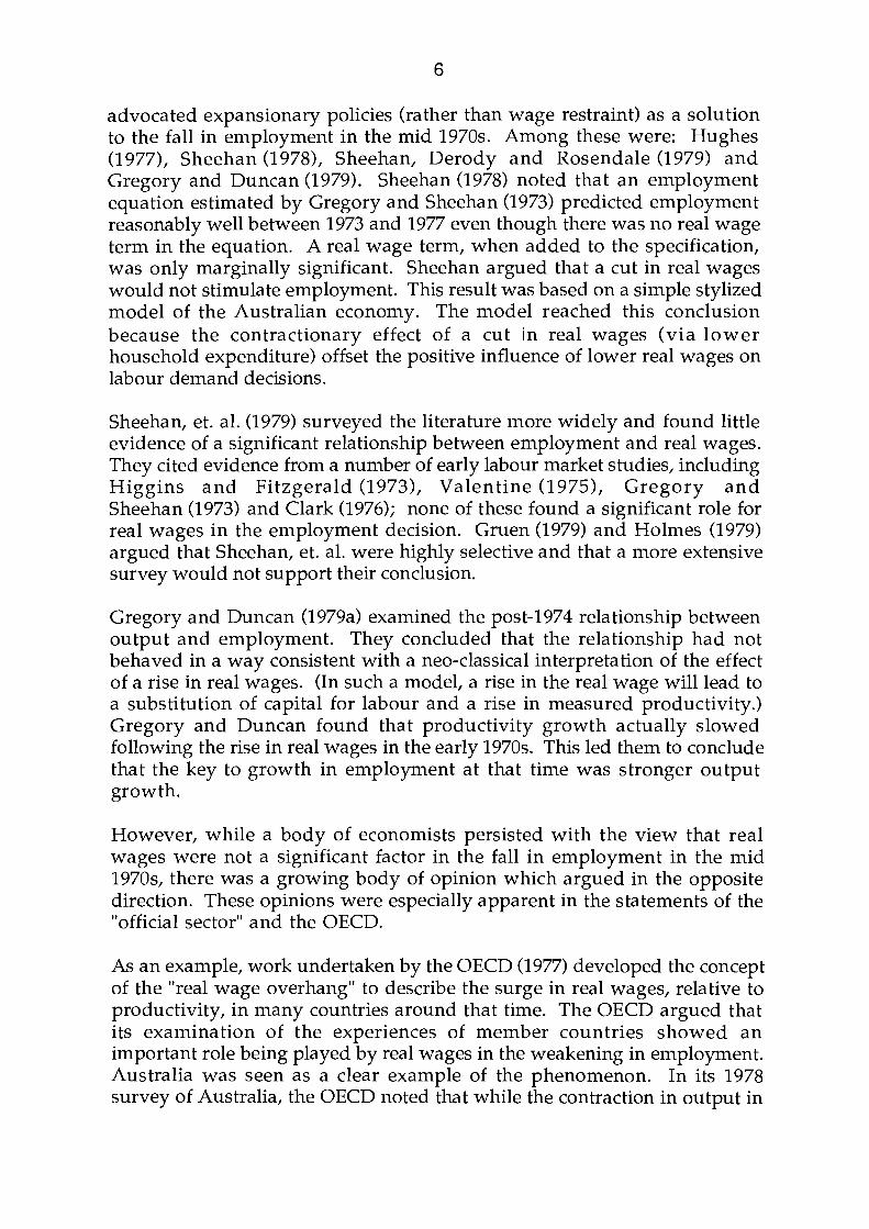
June 1974 to December 1975

Figure 2 plots the results of the simulation for the first period. The solid line on the Figure represents the actual path of employment; the dashed line represents the equation's estimate of what employment would have been if real unit labour costs had been constant; and the dotted line the estimate of employment had output grown on trend.

Consider the real wage simulation. If real unit labour costs had been unchanged in 1974/75, rather than rising sharply, then employment would have been much stronger during this period. Specifically, the estimates suggest that full-time employment in December 1975 would have been around 70,000, or 1-1/2 per cent, higher than it actually was. The estimated effect of the slowing in GOP growth was smaller. For the first part of the period, employment would have been stronger had GOP grown at trend. However, in the latter part of the period, when GDP growth exceeded trend, employment growth would have been a little weaker than actually observed.

These results suggest that the sharp rise in real unit labour costs was the major contributor to the downturn in en1ployment in 1974/75.

MILL.

5.20

5.15

5.10

5.05

5.00

Figure 2

EMPLOYMENT PATHS MILL.

~----------------------------------------r5.20

'-----------~~~~~~---------

. . . . .. . ·. · .. · .. ·· ... ·· ..

ACTUAL ··•···

1974

REAL WAGES

TREND GOP

1975

5.15

5.10

5.05

1 4

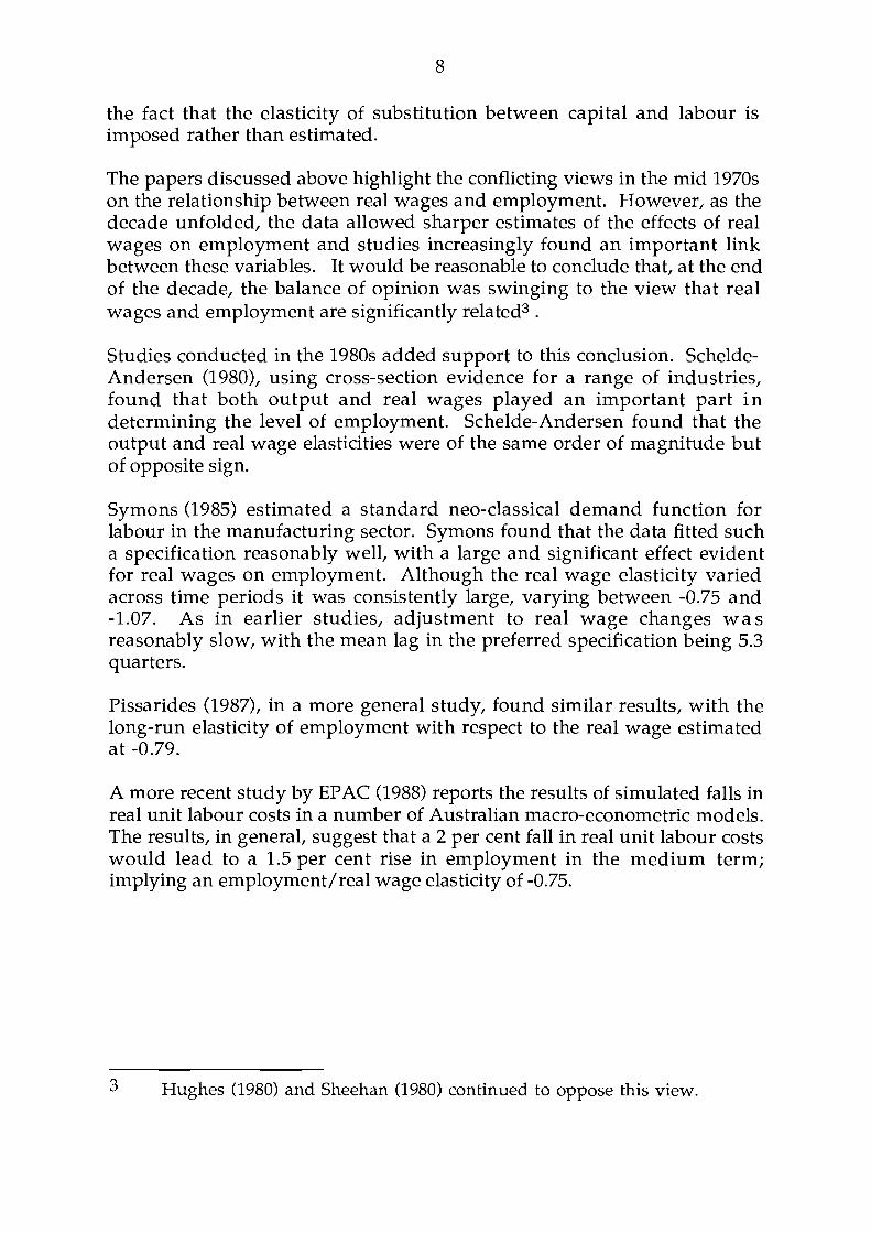
December 1981 to March 1983

Figure 3 illustrates the results of the same exercise for the downturn of the early 1980s. The effect of the slowing in GOP growth in this period was relatively more important than in 1974/75. This was due to the fact that the contraction in output in 1982/83 was much sharper than in 1974/75; as well, the large rise in real unit labour costs was unwound more quickly in the latter period. On the basis of the simulations, employment would have been 126,000 higher in March 1983 if output had not slowed below its trend rate. If real unit labour costs had not risen during this period, then employment would have been 154,000 higher than was observed.

Figure 3

EMPLOYMENT PATHS MILL. MILL.

5.5 ...---------------------,-5.5

5.4 ---·.:.:u ........ .._!If\.,., '7 .-: ••

5.3

5.2

5.1

1981 1982

The Period Since 1983

TREND REAL

...... WAGES -... ... ·····II .. ·· ........... . . . . . .. . . . TREND GDP

ACTUAL

5.4

5.3

5.2

The simulation exercises for this period suggest that much of the strength of employment can be attributed to the moderate wage outcomes. (Figure 4 provides details.) If real unit labour costs are held at a level that prevailed

1 5

immediately before the wage pause, then employment in December 1987 would have been 377,000 lower than the actual level. On the other h<lnd, employment would have only been 27,000 lower had GOP grown at trend (basically because growth in GDP was close to, or above, trend for most of that period).

MILL.

5.8

5.7

5.6

5.5

5.4

5.3

5.2

5.1

Figure 4

EMPLOYMENT PATHS MILL.

~-------------------------------------r5.8

.. .. . . . ' ....... .

SEP 1982

SEP 1983

. . . . ... . . .. ..

. . . .. ..

SEP 1984

.. . . ..

SEP 1985

TREND GOP

SEP 1986

5.7

5.6

5.5

5.4

5.3

5.2

These results suggest that the prolonged and large decline in real unit labour costs appears to have been the most important factor in the recent buoyancy of employment. The role of lower real wages in stimulating employment is highlighted in 1985/86. Between September 1985 and June 1986, GDP fell by 1-1/2 per cent. However, full-time employment grew by 2-3/4 per cent. This continued growth in employment in the face of a contraction in activity appears to have been due to the low and declining level of labour costs over the period.

The results of these simulations show that changes in both real wages and output have had important effects on employment in the 1970s and 1980s. The contraction in employment in 1974/75 could be labelled as largely

16

"Classical". A reduction in real unit labour costs in this period would have had a much larger effect on employment than a return to trend growth in GDP. The contraction in 1982/83 was a mix of both Keynesian and Classical features. Both a reduction in real unit labour costs and a return to trend GDP growth would have stimulated employment by around the same amount.

6. Conclusion

This paper has presented estimates of the effect of real wages and output on employment. It finds that both output and real wages have been important influences in employment over the past couple of decades. The estimated elasticities of employment with respect to output and real wages are roughly similar (though of opposite sign) and are well within the range of elasticities estimated in earlier studies.

Simulations with the estimated equation show that the large rise in real wages in 1974/75 and 1982/83 had an important bearing on the fall of employment in those years. Conversely, the prolonged fall in real wages since 1983 appears to have been an important factor in the strong employment growth since that time.

1 7

BIBLIOGRAPHY

A.G.P.S.(1977) Budget Statement No.2 1977/78.

Clark, C. (1976), "Wages, Profits and the Substitution Function", Economic Papers, no. 52, June.

Coghlan, P.L. (1978), "Simulation with the NIF Model of the Australian Economy", Simulation Special Interest Group Conference, Canberra.

Corden, W.M. (1978), "Wages and Unemployment in Australia", Presidential Address to the Seventh Conference of Economists, Sydney.

Dixon, P.B., B.R. Parmenter and J. Sutton, (1978), "Some Causes for Structural Maladjustment in the Australian Economy", Economic Papers, no. 57, January.

EPAC, (1988), Australia's Medium Term Growth Potential, AGPS Canberra.

Freebairn, J.W. (1977), "Do Wages Matter?" "Australian Economic Review, Third Quarter.

Freebairn, J.W. and G. Withers, (1977), "The Performance of Manpower Forecasting Techniques in Australian Labour Markets", Australian Bulletin of Labour, vol. 4, no. 1.

Gregory, R.G. and R.C. Duncan, (1979a), "Wages, Technology and Jobs", Australian Economic Review, First Quarter.

_____________ (1979b),"The Labour Market in the 1970s" in Reserve Bank of Australia(1979), Conference in Applied Economic Research,Sydney.

Gregory, R.G. and P.J. Sheehan, (1973), "The Cyclical Behaviour of the Australian Labour Market", Third Conference of Economists, Adelaide.

Gruen, F.H. (1979), "Comments on the Institute's Survey", Australian Economic Review, First Quarter.

Higgins, C.I. and V.M. Fitzgerald, (1973), "An Econometric Model of the Australian Economy", Journal of Econometrics, vol. 1, no. 3.

1 8

Higgins, C.l. (1973), "A Wage-Price Sector for a Quarterly Australian Model" in A.A. Powell and R. Williams (eds), Econometric Studies of Macro and Monetary Relation, North-Holland, Amsterdam.

Holmes,A.S. (1979), "What Do We Know?", Australian Economic Review, First Quarter.

Hughes, B (1977), "Policies for Full Employment", First National Congress of Labour Economists, Brisbane.

Hughes, B (1980), Exit Full Employment, Angus and Robertson, Sydney.

Johnston, H.N., R.B. Campbell and R.M. Simes, (1978), "The Impact of Wages and Prices on Unemployment", Economic Papers, no. 60.

Jonson, P.D., Mahar, K.L., Thompson, G.J., (1974), "Earnings and Award Wages in Australia", Australian Economic Papers, June 1974.

Jonson, P.D., R. Battellino and R. Campbell, (1978), "Unemployment, An Econometric Dissection", Reserve Bank of Australia, Research Discussion Paper no. 7802.

Kirby, M. (1981), "An Investigation of the Specification and Stability of the Australian Aggregate Wage Equation", Economic Record, no. 57.

OECD, (1977), Economic Outlook, July.

OECD, (1978), Australia, Economic Survey, April.

Parkin, M., (1973), "The Short-Run and Long-Run Trade-Offs between Inflation and Unemployment in Australia", Australian Economic Papers, December 1973.

Pissarides, C. (1987), "Real Wages and Unemployment in Australia", Centre for Labour Economics, London School of Economics Discussion Paper no. 286.

Reserve Bank of Australia, (1977), Annual Report.

Schelde-Andersen, P. (1980), "Real Wages, Inflation and Unemployment: A Case Study of the Australian Economy", University of Sydney min eo.

1 9

Sheehan, P.J. (1978), "Real Wages and Employment: an Alternative View", in Fisher, M.R. et.al. (1978), Real Wages and Unemployment, Centre for Applied Economic Research Paper no. 4, University of NSW.

Sheehan, P.J., B. Derody and P. Rosendale, (1979), "An Assessment of Recent Empirical Research Work Relevant to Macroeconomic Policy in Australia", Australian Economic Review, First Quarter.

Sheehan, P.J. (1980), Crisis in Abundance, Penguin Books, Australia.

Simes, R.M. and C.J. Richardson (1987), "Wage Determination in Australia", Economic Record, vol. 63.

Stan1mer, D. W. (1978), 'Real Wages and Unemployment", in Fisher, M.R. et.al. (1978), Real Wages and Unemployment, Centre for Applied Economic Research Paper No.4, University of NSW.

Symons, J. (1985), "Employment and the Real Wage in Australia" in Volker, P.A. ed, The Structure and Duration of Unemployment in Australia, Proceedings of a Conference, August.

Valentine, T. (1980), "The Effects of Wage Levels on Prices, Profits, Employment and Capacity Utilisation in Australia: An Econometric Analysis", Australian Economic Review, First Quarter.

Veale, J.M. (1985), "The Differential Effects of Macroeconomic Policy on Employment in States: Australia 1966-1978", PhD. Dissertation, University of NSW.

20

APPENDIX 1: Tests of the Lag Structure

The Koyck specification was tested against two less restrictive equations. The first had a general lag structure of the form:

lnEt = b0 + b1lnYt + b2lnYt-1 + b3lnWt + b4lnWt-1

+ b5 T + b6lnEt-1 + b7 lnEt-1 (2')

The second was an error-correction model of the form:

.6lnEt = c0 + q .6lnYt + c2 .6lnWt + c3lnEt-1 + c4lnY t-1

+ c5lnWt-1 + c 6T (2")

The error correction model (2") is nested in the more general model (2') and imposes the restrictions b2 = C4-CJ, b4 = C5-C2, and b7=0. The Koyck, in turn, is nested in both (2') and (2"). To get from the general specification to the Koyck, the following restrictions are imposed; b2 = 0, b4 = 0 and b7 = 0, while the following restrictions are imposed on the error correction model; c4-q = 0 and c5-c2 = 0. These restrictions are tested with a likelihood ratio test. Before presenting the test statistics, the estimates of 2' and 2" are reported in Tables 1 and 2, respectively.

Table 1

lnEt = b 0 + b1lnYt + b2lnYt-1 + b3lnWt + b4lnWt-1

+ b5 T + b6lnEt-1 + b7lnEt-2

Variable Coefficient Standard Error

1-D 0.91 0.35 lnYt 0.12 0.05 lnYt-1 0.003 0.05 lnWt -0.08 0.03 lnWt-1 -0.03 0.03 T -0.0005 0.0002

lnEt-1 0.85 0.13 lnEt-2 -0.41 0.37

RBAR2 =0.99 SEE= 0.005 SSR = 0.0013

DW1 = 1.98 Q(24) = 25.51

Durbin's h could not be calculated since T.Var(b6)>1.

21

The results reported above suggest that the restrictions imposed by the Koyck specification are reasonable; the coefficients b2, b4 and b7 are not significantly different from zero.

Table 2

~lnEt = c0 + q ~lnYt + c2~lnWt + c3lnEt-1 + c4lnYt-1

Variable

co WlnYt WlnWt lnEt-1 lnYt-1 T

lnWt-1

RBAR2 =0.47

DW = 1.98

Coefficient

0.95 0.12 -0.09 -0.19 0.12

-0.0005 -0.12

SEE= 0.004

Standard Error

0.32 0.05 0.03 0.05 0.03

0.0002 0.02

SSR = 0.0013

Q(24) = 26.23

As in the Koyck specification, all the variables are significant and of the right sign. The results are very close to those of the Koyck. The short-run output and real wage elasticities are 0.12 and -0.09 respectively (compared with 0.12 and -0.11 for the Koyck). The long-run output and real wage elasticities are 0.63 and -0.63 respectively (compared with 0.65 and -0.61 in the Koyck).

Table 3 reports the results of testing the restricted equations.

22

Table 3

Likelihood Ratio Test of a Restricted Equation Against a More General Specification.

Restriction2

General - Error Correction General - Koyck Error Correction - Koyck

Test Statistic3

0.90 0.49 0.54

Critical Value 95%

7.82 7.82 5.99

Neither the restrictions imposed by the error-correction specification nor those imposed by Koyck on the more general model can be rejected. Furthermore, the restrictions imposed by the Koyck on the error-correction specification could not be rejected. For this reason, the results reported in the body of the paper employ the Koyck specification.

2 This column refers to the restriction tested. The first (General- Error Correction) refers to the restrictions imposed by the error correction specification on the General model.

3 The test statistic is -2(Lr-Lu), where Lr is the log likelihood value of the specification which imposes the restriction while Lu is the log likelihood value of the unrestricted alternative. It is distributed x2(k) where k is the number of restrictions.

23

APPENDIX 2: Estimation with an Alternative Real Wage Measure

This appendix reports the results of estimating the preferred equation using real labour costs instead of real unit labour costs as the explanatory variable.

Variable

ao lnYt lnWt lnEt-1 T

RBAR2 = 0.99

h = 1.58

Table 1

Coefficient

0.55 0.14 -0.07 0.81

-0.0004

SEE= 0.005

Standard Error

SSR = 0.0015

0.31 0.03 0.01 0.04

0.0002

Q(24) ::: 27.15

The variables of interest are significant and of the right sign. The main difference between the results is that the coefficients on the real labour cost term and the time trend are lower. (The significance level of the trend has also fallen.)

A potential problem with this result is possible collinearity between the trend term, real labour costs and GDP. Both real labour costs and GDP have a strong upward trend for most of the period. To reduce this problem the trend term was dropped from the equation, yielding the results in table 2.

Variable

ao lnYt lnWt lnEt-1

RHO

RBAR2 =0.99

h = -0.006

Table 2

Coefficient

SEE= 0.005

1.17 0.10 -0.08 0.79

0.24

SSR = 0.0015

Q(24) = 22.65

Standard Error

0.36 0.02 0.02

0.063

0.14

24

The parameters on output and the real wage are now the same order of magnitude. The implied elasticities are both low relative to results reported earlier and to recent Australian studies. This is probably due to some remaining collinearity between GDP and real labour costs. (Examination of the correlation matrix suggests that this is the case.) This problem does not arise when real unit labour costs are used because they do not exhibit the strong upward trend of real labour costs (and output).

The important point to note from these estimations is that the qualitative relationship between employment and real wages is not dependent on the choice of a real wage variable. When the trend term is eliminated, real labour costs and output have a similar (though opposite) effect on employment. This was the case when real unit labour costs were used as the explanatory variable.

25

APPENDIX 3: Data used in the Study

F-time P-time Total Average Total Hours GDP Emp Emp Emp Hours Worked at

(a) (a) (a) (a) ('000 hours 1979/80 ('000) ('000) ('000) (hours /week) prices

/week ($mill) /worker) (b)

Sep.69 4623.6 572.7 5196.3 38.7 201096.8 21388 Dec. 69 4710.0 543.9 5253.9 38.8 203851.3 21513 Mar. 70 4758.5 562.2 5320.7 39.2 208571.4 21660 Jun. 70 4803.2 566.4 5369.6 38.9 208877.4 22429 Sep. 70 4838.6 571.5 5410.1 38.8 209911.9 22471 Dec. 70 4857.0 591.3 5448.3 38.8 211394.0 22803 Mar. 71 4884.0 598.2 5482.2 39.0 213805.8 23127 Jun. 71 4924.5 598.5 5523.0 38.8 214292.4 23413 Sep. 71 4951.7 580.8 5532.5 39.2 216874.0 24070 Dec. 71 4966.1 561.0 5527.1 38.9 215004.2 24047 Mar. 72 4968.2 568.8 5537.0 38.5 213174.5 23953 Jun. 72 4981.0 581.1 5562.1 38.8 215809.5 24711 Sep.72 4995.5 634.2 5629.7 38.6 217306.4 24461 Dec. 72 5022.6 652.5 5675.1 38.5 218491.4 25182 Mar. 73 5049.4 654.6 5704.0 37.7 215040.8 25810 Jun. 73 5051.7 659.4 5711.1 38.4 219306.2 25650 Sep. 73 5108.7 698.7 5807.4 38.3 222423.4 26159 Dec. 73 5134.8 701.7 5836.5 38.2 222954.3 26467 Mar. 74 5150.7 749.4 5900.1 38.7 228333.9 26398 Jun. 74 5176.1 729.6 5905.7 38.1 225007.2 26036 Sep. 74 5142.1 741.0 5883.1 37.6 221204.6 26308 Dec. 74 5085.3 790.2 5875.5 37.7 221506.4 26785 Mar. 75 5039.4 788.4 5827.8 37.6 219125.3 26767 Jun. 75 5070.8 765.6 5836.4 37.3 217697.7 27410 Sep. 75 5077.6 792.9 5870.5 36.9 216621.5 27118 Dec. 75 5090.2 840.9 5931.1 37.0 219450.7 27022 Mar. 76 5084.1 865.8 5949.9 37.1 220741.3 27721 Jun. 76 5091.5 873.0 5964.5 36.6 218300.7 28071 Sep. 76 5070.0 856.8 5926.8 36.5 216328.2 28195 Dec. 76 5067.7 874.8 5942.5 36.6 217495.5 28256 Mar. 77 5094.6 892.8 5987.4 36.0 215546.4 28136 Jun. 77 5096.4 909.3 6005.7 36.1 216805.8 28436 Sep. 77 5128.1 894.9 6023.0 36.2 218032.6 28376 Dec. 77 5041.2 942.9 5984.1 36.8 220214.9 28178 Mar. 78 5090.6 914.3 6004.9 33.5 201162.5 28563 Jun. 78 5118.0 921.8 6039.8 35.5 214412.9 28895 Sep. 78 5094.6 929.3 6023.9 35.7 215052.0 29669 Dec. 78 5111.9 931.6 6043.5 35.7 215754.1 29897 Mar. 79 5131.5 931.8 6063.4 35.8 217068.5 30374 Jun. 79 5135.0 950.7 6085.7 36.1 219692.6 30014

26

F-time P-time Total Average Total Hours GDP Emp Emp Emp Hours Worked at

(a) (a) (a) (a) 1979/80 ('000) ('000) ('000) (hours ('000 hours prices

/week /week) ($mill) /worker) (b)

Sep. 79 5163.4 951.1 6114.5 35.9 219510.6 30038 Dec. 79 5205.6 971.2 6176.8 35.8 221130.6 30596 Mar. 80 5242.7 982.7 6225.4 35.6 221624.2 30437 Jun. 80 5276.6 980.6 6257.2 34.7 217123.7 30773 Sep.80 5301.7 1016.4 6318.1 35.5 224292.6 30835 Dec. 80 5311.0 1023.0 6333.9 35.7 226121.4 31456 Mar. 81 5345.7 1027.3 6373.1 35.6 226881.2 31444 Jun. 81 5380.2 1039.6 6419.8 35.3 226617.8 31917 Sep.81 5396.7 1042.3 6439.0 35.3 227296.7 31995 Dec. 81 5400.5 1030.0 6430.5 35.4 227638.5 31914 Mar. 82 5420.1 1037.7 6457.8 35.4 228606.1 31970 Jun. 82 5383.3 1048.8 6432.1 35.2 226411.1 31996 Sep.82 5343.5 1070.6 6414.1 34.9 223853.3 31943 Dec. 82 5259.1 1093.5 6352.7 35.1 222978.6 31639 Mar. 83 5182.1 1101.9 6284.1 34.8 218685.5 31619 Jun. 83 5188.9 1077.9 6266.8 35.2 220591.4 31238 Sep.83 5224.0 1072.5 6296.4 35.2 221634.5 32327 Dec. 83 5262.3 1091.6 6353.9 35.4 224928.1 32556 Mar. 84 5293.8 1116.6 6410.4 35.1 225006.2 33579 Jun. 84 5348.2 1142.0 6490.2 35.5 230402.1 33971 Sep.84 5363.8 1157.4 6521.2 35.2 229545.1 34098 Dec. 84 5386.7 1152.4 6539.0 35.1 229520.1 34655 Mar. 85 5423.0 1164.0 6587.0 35.0 230543.8 34973 Jun. 85 5427.0 1181.5 6608.5 35.5 234600.6 35882 Sep.85 5496.4 1208.3 6704.7 34.8 233323.6 36697 Dec. 85 5545.6 1235.1 6780.7 35.1 238001.4 36284 Mar. 86 5618.4 1244.7 6863.1 35.3 242268.6 36490 Jun. 86 5642.8 1313.2 6956.0 34.2 237896.3 36175 Sep.86 5638.3 1316.9 6955.2 34.9 242735.3 36614 Dec. 86 5656.1 1334.5 6990.6 34.8 243271.7 37092 Mar. 87 5669.0 1368.9 7037.9 34.8 244918.9 37448 Jun. 87 5706.6 1383.2 7089.8 35.5 251686.7 38302 Sep.87 5732.5 1404.5 7137.0 34.6 246939.0 38237 Dec. 87 5752.9 1410.2 7163.1 35.2 252141.1 38807

a. Source A.B.S. Cat. No. 6202.0. b. Source A.B.S. Cat. No. 5206.0.

27

Average Average Real Nominal Real Productivity Unit Average

Labour Labour Earnings Costs Cost

(c) (c) (c) (c)

Sep. 69 98.7 100.4 98.3 93.9 Dec. 69 98.1 99.9 98.3 95.5 Mar. 70 98.5 99.1 99.4 98.2 Jun. 70 100.9 101.9 99.1 99.9 Sep. 70 101.0 102.2 98.9 101.1 Dec. 70 103.5 102.7 100.9 105.0 Mar. 71 105.2 103.1 102.1 110.1 Jun. 71 106.4 103.6 102.8 112.5 Sep.71 106.3 105.3 101.1 115.0 Dec. 71 107.6 105.9 101.7 116.3 Mar. 72 109.8 106.8 103.0 119.5 Jun. 72 109.8 108.3 101.5 122.5 Sep. 72 111.6 108.1 103.3 124.7 Dec. 72 112.5 111.0 101.4 127.6 Mar. 73 113.6 112.8 100.8 131.5 Jun. 73 115.4 112.3 102.8 138.5 Sep. 73 115.7 122.7 102.8 143.5 Dec. 73 117.8 112.8 104.5 149.0 Mar. 74 117.7 111.2 105.9 156.9 Jun. 74 119.8 109.3 109.6 165.1 Sep. 74 125.0 112.1 111.6 185.2 Dec. 74 126.9 113.8 111.6 195.8 Mar. 75 130.0 116.4 111.8 203.4 Jun. 75 127.3 118.6 107.5 206.0 Sep. 75 126.9 117.1 108.5 213.3 Dec. 75 126.2 116.9 108.0 222.7 Mar. 76 128.8 120.2 107.2 230.1 Jun. 76 130.3 121.5 107.3 239.8 Sep. 76 129.8 121.1 107.3 247.1 Dec. 76 132.1 122.4 108.0 252.7 Mar. 77 128.4 120.7 106.4 258.9 Jun. 77 134.1 123.6 108.5 268.0 Sep. 77 131.3 121.7 108.0 271.3 Dec. 77 132.6 120.4 110.2 278.9 Mar. 78 140.7 129.0 109.1 287.0 Jun. 78 135.4 126.2 107.3 290.9 Sep.78 135.7 128.0 106.1 296.1 Dec. 78 133.3 128.1 104.1 297.0

28

Average Average Real Nominal Real Productivity Unit Average

labour labour Earnings Costs Cost

(c) (c) (c) (c)

Mar. 79 135.5 128.7 105.4 310.6 Jun. 79 133.4 126.6 105.4 310.8 Sep.79 133.7 127.9 104.6 320.7 Dec. 79 136.7 130.1 105.2 327.0 Mar. 80 132.5 128.8 103.0 336.4 Jun. 80 139.0 133.3 104.3 346.1 Sep. 80 137.5 129.7 106.1 358.9 Dec. 80 137.8 131.6 104.8 371.4 Mar. 81 136.4 130.5 104.6 381.3 Jun. 81 141.5 133.5 106.1 396.2 Sep. 81 139.7 132.7 105.4 403.0 Dec. 81 140.1 132.2 106.1 416.4 Mar. 82 144.4 132.1 109.4 436.8 Jun. 82 145.0 132.1 109.9 455.2 Sep. 82 150.5 135.2 111.5 479.5 Dec. 82 148.3 135.8 109.3 485.2 Mar. 83 150.7 135.5 111.3 490.3 Jun. 83 144.1 138.0 104.5 481.2 Sep. 83 143.0 137.1 104.4 489.3 Dec. 83 141.9 136.0 104.4 498.8 Mar. 84 146.2 141.8 103.2 515.1 Jun. 84 143.8 138.7 103.8 525.6 Sep. 84 144.0 138.6 104.0 534.2 Dec. 84 145.0 141.7 102.5 540.0 Mar. 85 142.3 139.4 102.2 544.6 Jun. 85 145.1 143.1 101.5 560.8 Sep. 85 145.5 147.4 98.8 564.7 Dec. 85 145.0 142.6 101.7 573.8 Mar. 86 142.8 139.8 102.2 589.3 Jun. 86 146.6 144.6 101.4 588.2 Sep. 86 145.6 141.3 103.2 609.9 Dec. 86 143.5 142.4 100.9 612.4 Mar. 87 141.5 141.4 100.1 617.3 Jun. 87 141.2 144.3 97.9 627.1 Sep. 87 142.6 144.4 98.8 636.3 Dec. 87 141.9 144.3 98.4 652.4

c. Source: Treasury Round-up; Non-Farm, base 1966/67-1972/73 = 100.