A “warm path” for Gulf Stream-Troposphere1

interactions2

by Luke Sheldon, Arnaud Czaja?, Benoit Vanniere, Cyril3

Morcrette, Mathieu Casado, Doug Smith4

Authors’ adresses:5

• L. Sheldon, A . Czaja, Imperial College, Physics Department, Prince6

Consort Road, London SW7 2AZ, UK.7

• B. Vanniere, Department of Meteorology, University of Reading, Earley8

Gate, PO Box 243, Reading, RG6 6BB, UK.9

• C. Morcrette, D. Smith, Met Office, Fitzoy Road, Exeter, Devon EX110

3PB, UK.11

• M. Casado, Laboratoire des Sciences du Climat et de l’Environement,12

UMR8212, CEA-CNRS-UVSQ/IPSL, CEA Saclay, 91 191 Gif-sur-Yvette,13

France.14

?Corresponding author’s adress: A. Czaja, Imperial College, Physics De-15

partment, Prince Consort Road, London SW7 2AZ, United Kingdom, Tel.:16

+44-(0)20-75941789, Fax: +44-(0)20-75947772, e-mail: a.czaja@imperial.ac.uk17

1

Abstract18

Warm advection by the Gulf Stream creates a characteristic “tongue”19

of warm water leaving a strong imprint on the sea surface temperature20

(SST) distribution in the western North Atlantic. This study aims at21

quantifying the climatological impact of this feature on cyclones trav-22

elling across this region in winter using a combination of reanalysis23

data and numerical experiments.24

It is suggested that the Gulf Stream “warm tongue” is conducive25

to enhanced upward motion in cyclones because (i) it helps main-26

tain a high equivalent potential temperature of air parcels at low lev-27

els which favors deep ascent in the warm conveyor belt of cyclones28

and (ii) because the large SST gradients to the north of the warm29

tongue drive a thermally direct circulation reinforcing the transverse30

circulation embedded in cyclones. This hypothesis is confirmed by31

comparing simulations at high resolution (12km) from the Met Office32

Unified Model forced with realistic SST distribution to simulations33

with an SST distribution from which the Gulf Stream warm tongue34

was artificially removed or made much colder. It is also supported by35

a dynamical diagnostic applied to the ERAinterim dataset over the36

wintertime period (1979-2012).37

The mechanism of oceanic forcing highlighted in this study is as-38

sociated with weak air-sea heat fluxes in the warm sector of cyclones,39

which is in sharp contrast to what occurs in their cold sector. It is40

suggested that this “warm path” for the climatic impact of the Gulf41

Stream on the North Atlantic storm-track is not currently represented42

in climate models because of their coarse horizontal resolution.43

2

1 Introduction44

The Atlantic meridional overturning circulation leaves very sharp features in45

sea surface temperature (SST). In addition to the general surface warming of46

the North Atlantic compared to the North Pacific (e.g., Manabe and Stouffer,47

1988), the Florida Current and the separated Gulf Stream create a strong48

deformation of the sea surface isotherms, bringing poleward and eastward49

a “tongue” of warm water (Fig. 1a)1. To the north of this feature, very50

strong SST gradients are seen while to the south, the wrapping of the SST51

contours by the Gulf Stream recirculation and the action of mesoscale eddies52

tend to erode those gradients. In this study, we propose a new pathway53

through which these features impact the tropospheric circulation in the North54

Atlantic. In terms of the coupled atmosphere / Atlantic overturning system,55

this study thus focuses on the ocean → atmosphere pathway rather than on56

the atmospheric forcing of the Atlantic overturning circulation.57

The impact of the warm tongue of the Gulf Stream on air-sea interactions58

has been highlighted in many studies, in particular its role in setting a region59

of large net surface heating of the atmosphere, especially in winter (e.g., Gill,60

1982; Shaman et al., 2010). At this time of year, extra-tropical cyclones61

traveling from North America to the Atlantic ocean bring cold dry air of62

continental origin over the Gulf Stream warm tongue, leading to very large63

(in excess of hundreds of Wm−2) sensible and latent heat fluxes at the air-64

sea interface. The impact of the warm tongue above the marine boundary65

1Although only shown here on a given day, this feature persists in the climatological

wintertime mean –not shown

3

layer has traditionally been understood as a response to these large fluxes66

and their associated shallow heating of the troposphere (Hoskins and Karoly,67

1981; Kushnir et al., 2002).68

The discussion above relates to the cold sector of cyclones, but the pres-69

ence of the Gulf Stream warm tongue can also influence the atmosphere in70

their warm sector. Indeed, the latter is where air masses of low-latitude ori-71

gins are advected poleward and upward, in a manner sometimes referred to72

as a “warm conveyor belt” (WCB, see for example Browning, 1990; Schemm73

et al., 2013). This motion is associated with weak turbulent heat fluxes at74

the sea surface, even possibly directed downward (e.g., Boutle et al., 2011),75

but it leads to a deep heating of the troposphere through latent heat release76

(Hoskins and Valdes, 1990). To focus in this study on the warm sector, we77

simulate the response of an extra-tropical cyclone to different SST config-78

urations in the western North Atlantic, with and without the Gulf Stream79

warm tongue, and focus on the induced changes in upward motion (section80

2). These simulations are carried out at high spatial resolution (12km, i.e.81

“high” in the context of global climate models) because it is known that82

frontal circulations, where the upward motion is concentrated, are too weak83

in coarse resolution models (e.g., Bauer and del Genio, 1996; Catto et al.,84

2010; Willison et al., 2013). In section 3 we apply a dynamical diagnostic to85

atmospheric reanalyses data during the wintertime to assess the relevance of86

the mechanism in Section 2 to the climatology. A summary and a discussion87

are offered in section 4.88

4

2 Experiments with the Met Office Unified89

Model90

2.1 Model set-up91

The Met Office Unified Model (hereafter MetUM) has been run in a global92

configuration on a global grid of horizontal resolution 0.37 × 0.56 (≈ 4093

km) to generate the boundary conditions of a nested North Atlantic domain94

(≈ 12km)2. The MetUM is a finite-difference model which solves the non-95

hydrostatic, deep-atmosphere dynamical equations. The parameterization of96

physical processes includes longwave and shortwave radiation, boundary layer97

mixing, convection, and cloud cover and large-scale precipitation. Specifically98

we ran the version MetUM 7.3, with the set up used in Martinez-Alvarado et99

al. (2014). The reader is referred to this paper for details about the model.100

The model was initialized on January 14th 2004 at 1200 UTC and inte-101

grated over 72 hours, using initial conditions from the ECMWF operational102

analysis. On January 15th 1200 UTC (i.e., 24h into the simulation), a large103

tropopause trough was centered on the east coast of North America. The104

upper-level cyclone was associated with a low-level cyclone in the Gulf Stream105

basin with lowest pressure equal to 988 hPa. The low-level cyclone deepened106

by 45 hPa over the course of the following 24 hours. We have simulated the107

passage of this cyclone using three different SST configurations (all constant108

2The North Atlantic domain has a non uniform grid which is obtained by rotation of the

uniform equatorial grid to the midlatitudes (typical grid point spacing being ≈ 0.1). It

extends eastward from 20E up to 70E and westward from 7W up to 12W , depending

on latitude (the latter itself ranges from as low as 10N to as high as 80N).

5

in time). The first, named CNTL, uses the observed SST distribution on109

January 14 2014 at 1200 UTC. The second, named SMTH, uses a smoothed110

version of the CNTL SST. The smoothing was generated using a spatial fil-111

ter in which each point is a weighted average of itself and its four immediate112

neighbours (in the ratio 1:1/4). The filter was applied iteratively 3000 times113

in a box centered on the Gulf Stream basin with a Gaussian transition to114

the region outside the box where no smoothing is applied. This experiment115

is specifically aimed at “removing” the Gulf Stream warm tongue in order116

to see its impact on the warm sector of the cyclone. Finally, in a third117

experiment, named COOL, we lower uniformly the SST by 3K over the en-118

tire nested domain. This experiment is carried out to investigate the role of119

the absolute temperature of the warm tongue, as opposed to the role of the120

SST gradient north of this feature. All simulations share the same lateral121

boundary conditions and differ only by the prescribed SST. The three SST122

distributions can be compared in Fig. 1 (panels a, b, c for CNTL, SMTH123

and COOL, respectively, and panel d for the difference CNTL-SMTH).124

2.2 Results125

At 24h into the simulation, a well defined region of upward motion has de-126

veloped over the Northwest Atlantic at midlevels, as indicated by the area127

with positive upward velocity near 37N, 68W in Fig. 2a (red colours). One128

also notices the presence of another well developed region of ascent east of129

60W , which is the signature of the previous cyclone having travelled across130

the Gulf Stream at t < 0. Both features are seen in Fig. 2b to be associated131

6

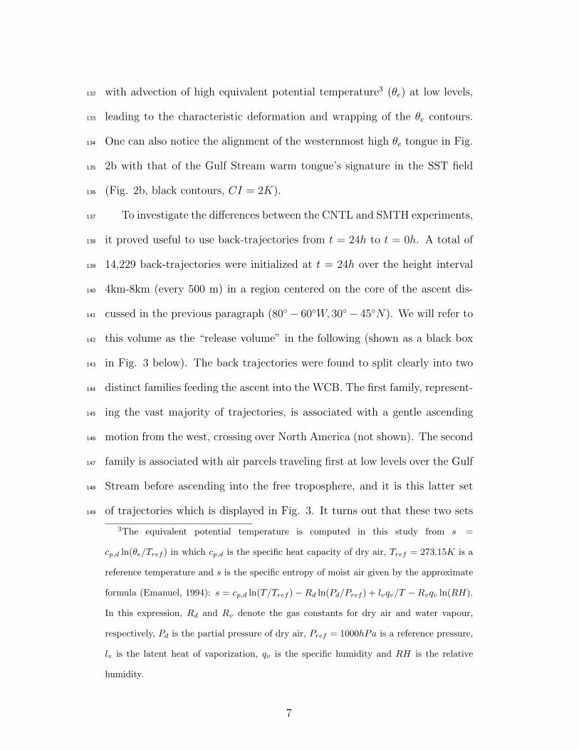
with advection of high equivalent potential temperature3 (θe) at low levels,132

leading to the characteristic deformation and wrapping of the θe contours.133

One can also notice the alignment of the westernmost high θe tongue in Fig.134

2b with that of the Gulf Stream warm tongue’s signature in the SST field135

(Fig. 2b, black contours, CI = 2K).136

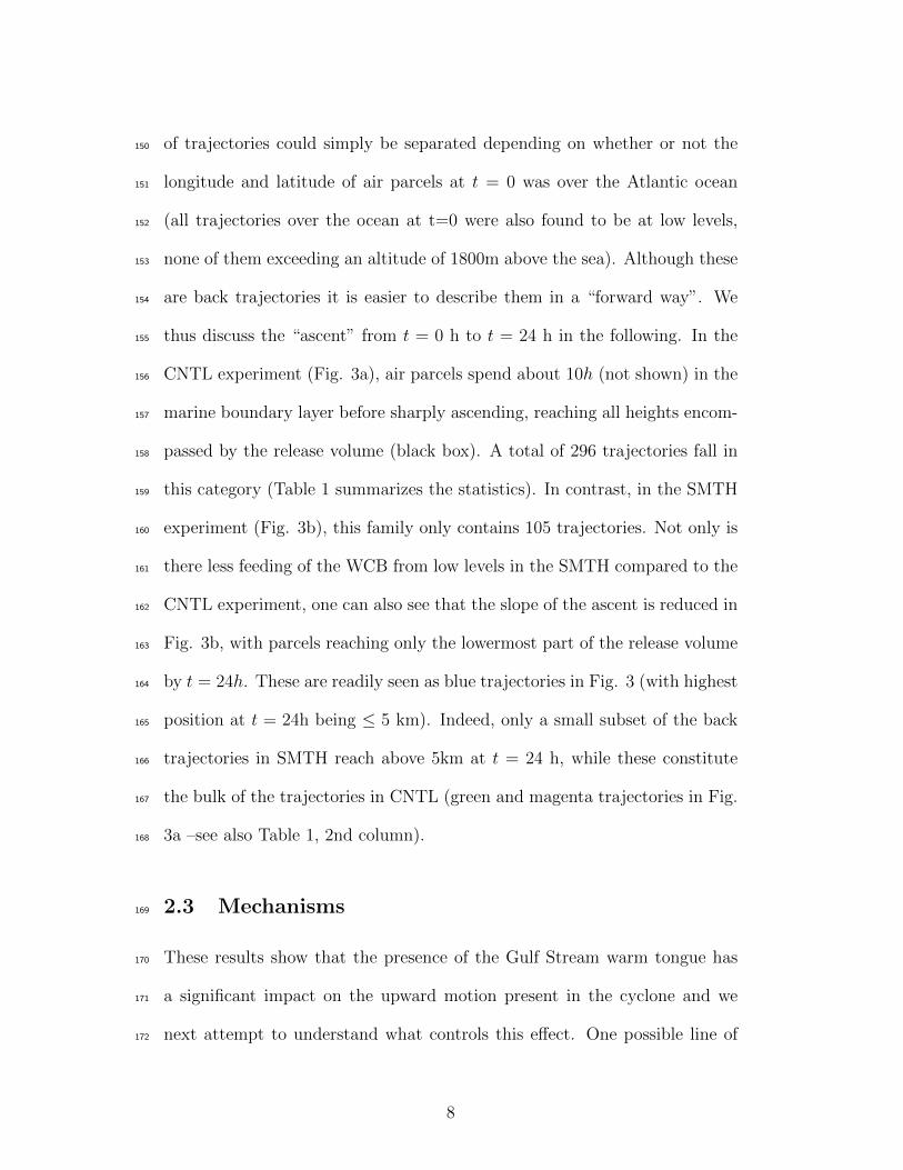
To investigate the differences between the CNTL and SMTH experiments,137

it proved useful to use back-trajectories from t = 24h to t = 0h. A total of138

14,229 back-trajectories were initialized at t = 24h over the height interval139

4km-8km (every 500 m) in a region centered on the core of the ascent dis-140

cussed in the previous paragraph (80− 60W, 30− 45N). We will refer to141

this volume as the “release volume” in the following (shown as a black box142

in Fig. 3 below). The back trajectories were found to split clearly into two143

distinct families feeding the ascent into the WCB. The first family, represent-144

ing the vast majority of trajectories, is associated with a gentle ascending145

motion from the west, crossing over North America (not shown). The second146

family is associated with air parcels traveling first at low levels over the Gulf147

Stream before ascending into the free troposphere, and it is this latter set148

of trajectories which is displayed in Fig. 3. It turns out that these two sets149

3The equivalent potential temperature is computed in this study from s =

cp,d ln(θe/Tref ) in which cp,d is the specific heat capacity of dry air, Tref = 273.15K is a

reference temperature and s is the specific entropy of moist air given by the approximate

formula (Emanuel, 1994): s = cp,d ln(T/Tref )− Rd ln(Pd/Pref ) + lvqv/T − Rvqv ln(RH).

In this expression, Rd and Rv denote the gas constants for dry air and water vapour,

respectively, Pd is the partial pressure of dry air, Pref = 1000hPa is a reference pressure,

lv is the latent heat of vaporization, qv is the specific humidity and RH is the relative

humidity.

7

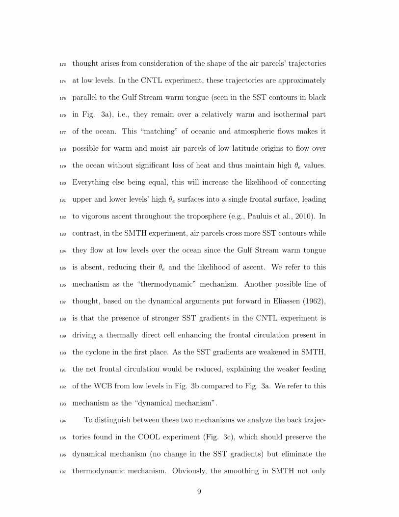
of trajectories could simply be separated depending on whether or not the150

longitude and latitude of air parcels at t = 0 was over the Atlantic ocean151

(all trajectories over the ocean at t=0 were also found to be at low levels,152

none of them exceeding an altitude of 1800m above the sea). Although these153

are back trajectories it is easier to describe them in a “forward way”. We154

thus discuss the “ascent” from t = 0 h to t = 24 h in the following. In the155

CNTL experiment (Fig. 3a), air parcels spend about 10h (not shown) in the156

marine boundary layer before sharply ascending, reaching all heights encom-157

passed by the release volume (black box). A total of 296 trajectories fall in158

this category (Table 1 summarizes the statistics). In contrast, in the SMTH159

experiment (Fig. 3b), this family only contains 105 trajectories. Not only is160

there less feeding of the WCB from low levels in the SMTH compared to the161

CNTL experiment, one can also see that the slope of the ascent is reduced in162

Fig. 3b, with parcels reaching only the lowermost part of the release volume163

by t = 24h. These are readily seen as blue trajectories in Fig. 3 (with highest164

position at t = 24h being ≤ 5 km). Indeed, only a small subset of the back165

trajectories in SMTH reach above 5km at t = 24 h, while these constitute166

the bulk of the trajectories in CNTL (green and magenta trajectories in Fig.167

3a –see also Table 1, 2nd column).168

2.3 Mechanisms169

These results show that the presence of the Gulf Stream warm tongue has170

a significant impact on the upward motion present in the cyclone and we171

next attempt to understand what controls this effect. One possible line of172

8

thought arises from consideration of the shape of the air parcels’ trajectories173

at low levels. In the CNTL experiment, these trajectories are approximately174

parallel to the Gulf Stream warm tongue (seen in the SST contours in black175

in Fig. 3a), i.e., they remain over a relatively warm and isothermal part176

of the ocean. This “matching” of oceanic and atmospheric flows makes it177

possible for warm and moist air parcels of low latitude origins to flow over178

the ocean without significant loss of heat and thus maintain high θe values.179

Everything else being equal, this will increase the likelihood of connecting180

upper and lower levels’ high θe surfaces into a single frontal surface, leading181

to vigorous ascent throughout the troposphere (e.g., Pauluis et al., 2010). In182

contrast, in the SMTH experiment, air parcels cross more SST contours while183

they flow at low levels over the ocean since the Gulf Stream warm tongue184

is absent, reducing their θe and the likelihood of ascent. We refer to this185

mechanism as the “thermodynamic” mechanism. Another possible line of186

thought, based on the dynamical arguments put forward in Eliassen (1962),187

is that the presence of stronger SST gradients in the CNTL experiment is188

driving a thermally direct cell enhancing the frontal circulation present in189

the cyclone in the first place. As the SST gradients are weakened in SMTH,190

the net frontal circulation would be reduced, explaining the weaker feeding191

of the WCB from low levels in Fig. 3b compared to Fig. 3a. We refer to this192

mechanism as the “dynamical mechanism”.193

To distinguish between these two mechanisms we analyze the back trajec-194

tories found in the COOL experiment (Fig. 3c), which should preserve the195

dynamical mechanism (no change in the SST gradients) but eliminate the196

thermodynamic mechanism. Obviously, the smoothing in SMTH not only197

9

alters the SST gradient but also the absolute SST values, with a cooling on198

the warm flank of the Gulf Stream and a warming on its poleward flank. It199

is for this reason that we chose to lower the SST by 3 K in COOL so that the200

absolute value of SST over the Gulf Stream warm tongue remains compara-201

ble in both experiments. As can be seen in Fig. 3c, the COOL experiment is202

somewhat in between the CNTL and SMTH. A total of 169 back trajectories203

were obtained, as opposed to 105 and 296 in SMTH and CNTL, respectively.204

Breakdown of the initial heights in each of these experiments in Table 1 (2nd205

column) indicates that the bulk of the trajectories originates above 5 km in206

COOL (green and magenta trajectories), as in CNTL, in contrast to SMTH207

where we saw in the previous section that the bulk of trajectories originated208

from below 5 km (blue trajectories). This suggests that the partitioning be-209

tween bottom or top heavy feeding of the ascent from low levels is primarily210

set by the SST gradient. In addition, we note that the absolute numbers of211

trajectories is much reduced in COOL compared to CNTL, with only 14 tra-212

jectories originating above 7 km in COOL compared to 54 in CNTL. Thus the213

ability of air parcels to join in the WCB is sensitive to the absolute SST over214

the warm tongue, demonstrating an important role for the thermodynamic215

mechanism.216

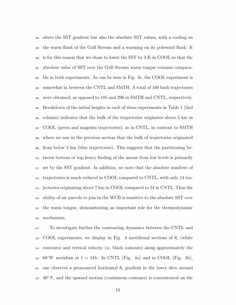
To investigate further the contrasting dynamics between the CNTL and217

COOL experiments, we display in Fig. 4 meridional sections of θe (white218

contours) and vertical velocity (w, black contours) along approximately the219

68W meridian at t = 24h. In CNTL (Fig. 4a) and in COOL (Fig. 4b),220

one observes a pronounced horizontal θe gradient in the lower 4km around221

40N , and the upward motion (continuous contours) is concentrated on the222

10

equatorward side of this region. The upward motion (continuous black line)223

is broader both in latitude and height in the CNTL experiment, and it is224

also larger in magnitude compared to the COOL experiment. The down-225

ward motion (dashed black contours) is comparatively little affected and is226

overall weaker (note that the contour interval is four times greater for w > 0227

than w < 0 in Fig. 4). We have superimposed in both panels the difference228

in θe between these two experiments (CNTL-COOL) as a colour field. The229

resulting θe anomalies are on the order of the prescribed SST change on the230

warm side of the front (a few K), i.e. comparable to the vertical variations231

in θe there. In other words, the surface heating and moistening driven by the232

larger SSTs in CNTL leads to a significant modulation of the moist stratifi-233

cation on the warm side of the front –note for example the more pronounced234

folding of the 310K contour in Fig. 4a compared to Fig. 4b. We also note235

that the contours of w are also a bit more jagged in Fig. 4a compared to Fig.236

4b, a feature even more pronounced in a zonal section along approximately237

38N (not shown). This suggests that some form of resolved instability might238

be at work in CNTL but we have not pursued this issue further.239

In summary, both the “thermodynamical” and “dynamical” mechanisms240

are acting constructively and are needed to explain the differences in circula-241

tion between CNTL and SMTH. This likely reflects the particular geometry242

of the problem: trajectories of air parcels at low levels have a similar orienta-243

tion to the warm tongue of the Gulf Stream which allows them to maintain244

high θe while flowing just above the ocean while, at the same time, the large245

SST gradients to the north of the warm tongue reinforce the thermally direct246

circulation at the front in which the parcels are embedded. A schematic of247

11

this idea is provided in Fig. 5.248

2.4 Dependence on spatial resolution249

We have repeated the CNTL, SMTH and COOL experiments (and the back250

trajectory analysis) at an horizontal resolution of 40km rather than 12km.251

As can be seen in the statistics summary in Table 1, there is a large and252

systematic reduction in the number of trajectories feeding the ascent from253

low levels in all experiments when going from 12km to 40km. Focusing254

first on the bulk trajectories (rows labelled “all”), we see that in COOL, the255

numbers decrease by a factor of two while in CNTL and SMTH, they decrease256

by approximately a factor of three. Separate examination of the trajectories257

reaching above and below 5 km (i.e., trajectories whose initial position at258

t = 24h is above or below 5 km) indicates even more drastic changes. Indeed,259

in all experiments at 40 km resolution the number of trajectories originating260

below 5 km is larger than that originating above this level. As was discussed261

in section 2.3, this situation only occured in the SMTH experiment at 12 km262

resolution. The most dramatic illustration of the impact of resolution is the263

complete absence at 40 km of trajectories originating above 7 km at t=24h,264

while such trajectories represented 8 % and 18 % of the population for the265

COOL and CNTL experiments at 12 km, respectively.266

The only difference between a given experiment at 12 and 40km is atmo-267

12

spheric resolution4, as the SSTs are identical (not shown)5. To investigate268

further the reasons for the decrease in numbers seen in Table 1 when decreas-269

ing the spatial resolution, we display in Fig. 6 the probability distribution270

functions (PDFs) of the Lagrangian vertical velocities wL along the set of271

trajectories (the latter was estimated from the height zL of the parcels ac-272

cording to wL = dzL/dt). In the CNTL experiment (Fig. 6a), we observe273

a very different PDF at 12 km (grey) compared to 40 km (dashed black).274

The distribution is broader at 12km, with a more elongated tail on both the275

updraft and downdraft side (not the log scale used). Nevertheless, and some-276

what surprisingly, the updrafts occupy a larger fraction of the distribution277

at 40km (i.e., the bins with wL > 0 add up to 84 % of the distribution at278

40km but to 70 % at 12km). As can be seen in Fig. 6a, this results from279

the presence of more moderate updraft and less moderate downdrafts (taking280

wL = 0.25 m/s as a reference value) at 40km compared to 12 km. Similar281

results apply to the PDFs in the COOL (Fig. 6c) and SMTH (Fig. 6b)282

experiments.283

This analysis suggests that the larger feeding of midlevel ascent from284

low levels at 12 km compared to 40 km occurs in conjunction with a more285

frequent occurrence of wL > 0.25 m/s and wL < 0. This is not only observed286

when comparing the 12 and 40 km experiments, but also when comparing287

4Note that the 40km set-up has a higher vertical resolution with 38 levels between

the sea surface and 10km while there are 22 such levels for the 12 km set-up (overall the

number of levels is 70 for the 40km set-up and 38 for the 12 km set-up).5SSTs at 40 km were obtained by interpolation of the operational 25km - ECMWF

SSTs, as was done to generate the CNTL SST at 12 km. The analog of Fig. 1 at 40km

resolution is indistinguishable from that at 12 km (not shown).

13

experiments at a given resolution. For example, the reduction in the number288

of overall trajectories from 296 to 105 between CNTL and SMTH at 12 km289

resolution (and the shift from a top heavy to bottom heavy partitioning –290

see section 2.3) also goes in hand with a reduction in these more intense291

updrafts/downdrafts (compare the grey curves in Fig. 6a and 6b). The292

causality is not entirely clear at this stage though because events with more293

intense vertical motions are rare. Further work is needed to investigate this294

point further and also to explain the dynamical origin of these events.295

3 Analysis of the ERAinterim dataset296

The previous section suggests that the Gulf Stream warm tongue has an im-297

pact on the ascending motion embedded in cyclones traveling in the north-298

west Atlantic, but it was only based on a single case study. To investigate299

whether this impact can also be detected in a climatological sense, we now300

analyze the ERAinterim reanalysis datasets over the 1979-2012 period (De-301

cember through February). This dataset provides a gridded estimate of the302

state of the global atmosphere (here used on the native T255 truncation,303

approximately equivalent to a 80km horizontal resolution) through a four304

dimensional variational analysis and a 12-hour analysis window (Dee et al.,305

2011). We do not expect the reanalysis data to capture the dynamics present306

in the simulations discussed in Section 2 because of its relatively coarse res-307

olution. Our strategy is instead to use the ERA interim data to provide an308

estimate of the environment in which the smaller scale dynamics, and espe-309

cially the enhanced ascent for air parcels flowing at low levels over the Gulf310

14

Stream warm tongue, might develop.311

Specifically, we follow the framework of Shutts (1990), and compute tra-312

jectories along which enhanced ascent is expected to be found, given some313

environmental conditions. The trajectories in question are computed from314

the assumed conservation of the two components of absolute momentum (M315

and N) from an initial position at longitude λo and latitude φo. These com-316

ponents can be computed from:317

M = 2Ω sinφa(λ− λo) cosφ+ v, (1)318

N = 2Ωa(cosφ− cosφo)− u (2)

in which Ω is the Earth’s rotation angular frequency, a is the Earth’s radius,319

λ and φ denote longitude and latitude, respectively, and u and v are the320

zonal and meridional wind components, respectively. The assumption of321

conservation of M and N along the trajectory requires slow variations of322

the geostrophic flow in a particular direction, as occurs for example along a323

frontal region (Shutts, 1990). In addition, the method also assumes that the324

ascent occurs on a shorter timescale than the typical timescale of evolution325

of the system (Gray and Thorpe, 2001). As emphasized by Gray and Thorpe326

(2001), both assumptions are only approximately satisfied in Nature so the327

results have to be treated with caution.328

The calculation can be summarized as follows. At a given low level grid-329

point A (longitude λo, latitude θo) and time to, we compute the intersection of330

the M and N surfaces. This intersection defines a line as one moves upward,331

and we define point B as the intersection of this line with the tropopause332

(the latter was simply identified by the 2PV unit contours, following Hoskins333

15

et al., 1985). The results in Section 2 suggested that the presence of high334

θe values at low levels is instrumental in setting the strength of the ascent.335

Motivated by this, we thus record the difference ∆θe,336

∆θe(λo, φo, to) = θe(A, to)− θe(B, to) (3)

Our working hypothesis is that, based on the simulations in Section 2, situa-337

tions in which ∆θe is positive should be found more frequently over the Gulf338

Stream warm tongue than over the surrounding waters.339

To test this hypothesis, let us first consider the ideal scenario in which air340

parcels flowing over the Gulf Stream warm tongue are very nearly thermody-341

namically adjusted to the ocean. In that case we can plausibly set θe(A, to)342

to be the equivalent potential temperature that an air sample would have if343

its temperature were equal to the SST and its relative humidity were equal to344

80 % (we denote this value by θe,eq in the following). The fraction of the time345

in winter when the condition ∆θe > 0 is met with this particular choice is346

shown in Fig. 7a. Strikingly, and in support of our hypothesis, one observes347

that occurrences are maximized along the Gulf Stream warm tongue, and348

much reduced elsewhere. Along the warm tongue, values as high as 40% are349

found.350

The above calculation is clearly an overestimation since not all air streams351

at low levels are close to thermodynamic equilibrium with the ocean. To con-352

sider a more realistic situation we thus set, in a second calculation, θe(A, to)353

to be the actual equivalent potential temperature at 950hPa. The result-354

ing map of occurrence is displayed in Fig. 7b. As expected the magnitudes355

drop compared to Fig. 7a (note the factor of 4 difference in the colorbar356

16

between the two panels), but one still observes a clear maximum along the357

Gulf Stream warm tongue.358

In summary, application of a dynamical diagnostic to the environmental359

conditions provided by the ERA interim data suggest that the Gulf Stream360

warm tongue is the region where vigorous ascent from low levels should be361

most frequently observed in the Northwest Atlantic in winter. The occurrence362

of such events is comparable (5 − 10% of the wintertime based on Fig. 7b)363

to that of the surface fronts detected over the Gulf Stream (e.g., Berry et al.,364

2011) so they must be an intrinsic feature of their dynamics in that region.365

4 Summary and discussion366

It has been known for many years that individual cyclones are sensitive to367

the distribution of SST in the Northwest Atlantic (e.g., Kuo et al. 1991; Reed368

et al., 1993; Booth et al., 2012). In addition, it is also well established that369

the climatological distribution of WCBs in the Northern hemisphere winter370

peaks over the Gulf Stream warm tongue (e.g., Madonna et al., 2014), and371

that phenomenon associated with vigorous updrafts such as lightning strikes372

are preferentially found over the Gulf Stream in winter (Christian et al.,373

2003). The novelty of our study is to suggest that these features are influ-374

enced by the particular geometry of air parcels’ trajectories embedded in the375

cyclone at low levels and how these relate to the underlying SST distribu-376

tion. Specifically, we proposed that the alignment of air parcels’ trajectories377

at low levels with the Gulf Stream warm tongue and the associated SST378

gradients on its poleward flank is key to the enhancement of upward motion379

17

in cyclones traveling over the northwest Atlantic (see schematic in Fig. 5).380

It was further argued that both thermodynamical (absolute temperature of381

the warm tongue) and dynamical (strength of the SST gradient) effects were382

needed to produce this enhancement. While this conclusion was based on a383

single case study using high resolution (12km) simulations with the MetUM384

model, it was also supported by the application of a dynamical diagnostic to385

a climatological dataset (ERA-interim reanalysis, 1979-2012, wintertime).386

Our study raises an important question regarding the spatial resolution387

needed to simulate accurately the response of the atmosphere to the presence388

of the Gulf Stream and, more generally, the climatic impact of the extra-389

tropical oceans. To illustrate why resolution might be of importance, let’s390

use the results of the back trajectory analysis in section 2. It can reasonably391

be argued that the diabatic heating in the ascending branch of the simulated392

cyclone scales with the upward mass transport of this branch, as the diabatic393

heating results from the condensation of water vapour carried by the flow.394

In turn, we expect this upward mass transport to scale with the number of395

trajectories feeding the ascent. Under this assumption, the difference in the396

number of trajectories found under two different SST configurations provides397

a measure of oceanic forcing6 . This idea is applied in Fig. 8 by using the398

numbers in Table 1 for back trajectories starting above 5 km at t = 24 h,399

in an attempt to estimate an upper level oceanic forcing. In this figure we400

normalized the number of trajectories by that found in the CNTL experiment401

6This upper level forcing can be thought of as “thermal” if phrased in terms of latent

heat release as was just done. It can also be thought of as mechanical if it is considered

from the point of view of the perturbed ascending motion –see Parfitt and Czaja (2015).

18

at 12 km (red circle on the left column). The green arrow indicates the402

normalized change in the number of trajectories when comparing a realistic403

(CNTL) and a smoothed (SMTH) SST distribution at 12 km (left column)404

or 40 km (right column) –likewise for the blue arrow and the response of the405

atmosphere to colder SST anomalies in the COOL experiment compared to406

CNTL. It is readily seen that the length of the arrow is reduced by a about407

a factor of 4 (green) and a factor 3 (blue) at 40km compared to 12 km, i.e.,408

the upper level oceanic forcing roughly scales with the horizontal resolution409

in both perturbed experiments (CNTL v.s SMTH and CNTL v.s COOL).410

The lower end of resolution considered in this study (40 km) is still much411

higher than that used in most climate models. An extrapolation of the re-412

sults in Fig. 8 would suggest that upper level oceanic forcing would be almost413

inexistant for grid sizes on the order of a few 100 km. A possible implica-414

tion of our study is thus that climate models with grid sizes of several 100km415

might not be able to simulate accurately the impact of the Gulf Stream warm416

tongue on the warm sector of cyclones (we refer to this impact as a “warm417

path” for the oceanic influence). It is likely that this is the primary reason418

why the response of Atmospheric General Circulation Models (AGCMs) to419

extra-tropical SST anomalies has so far proven not to be robust (Kushnir et420

al., 2002). Indeed, AGCMs with grid sizes on the order of 100km or more421

can only represent the shallow thermal forcing associated with air-sea inter-422

actions in the cold sector of cyclones (a “cold path” to keep with the above423

terminology –see Vanniere et al., 2016) and it is known that the response of424

the atmosphere to such heating is quite sensitive to the model background425

state (e.g., Ting and Peng, 1995; Kushnir et al., 2002). In contrast, the warm426

19

path highlighted in our study consists of a modulation of the upward motion427

and latent heating, and thereby represents a direct forcing of the upper levels428

heat and vorticity budgets. We thus expect this pathway of oceanic influence429

to be more robust. Recent experiments by Smirnov et al. (2015) suggest that430

as the horizontal resolution of an AGCM is increased from about 100km to431

25km, its response to the same SST anomaly becomes fundamentally differ-432

ent in character (from a weak to a strong upper level response). This, we433

suggest, could be the signature of the SST forcing switching from cold to434

warm path in this model.435

Acknowledgments: This work is part of Luke Sheldon’s PhD funded by436

the Grantham Institute at Imperial College and in collaboration with the437

UK Met Office through a CASE studentship. Benoit Vanniere is funded by438

a grant from the Natural Environment Research Council NE/J023760/1.439

References440

[1] Bauer, M. and A. D. Del Genio, 2006. Composite analysis of winter441

cyclones in a GCM: influence on climatological humidity, J. Clim., 19,442

1652-1672.443

[2] Berry, G. B., Reeder, M. J., Jakob, C., 2011. A global climatology of444

atmospheric fronts, Geopys. Res. Let. 38 (4), L04809.445

[3] Booth J. F., L. Thompson, J. Patoux, K. A. Kelly, 2012: Sensitivity446

of midlatitude storm intensification to perturbations in the sea surface447

temperature near the Gulf Stream, Mon. Wea. Rev., 140, 1241-1256.448

20

[4] Boutle, I., S. E. Belcher and R. S. Plant, 2011. Moisture transport in449

midlatitude cyclones, Q. J. R. Meteorol. Soc. 137, 360-373.450

[5] Browning, K. A., 1990. Organization of clouds and precipitation in451

extratropical cyclones. Extratropical Cyclones: The Erik H. Palmen452

Memorial Volume, C. Newton and E. Holopainen, Eds., Amer. Me-453

teor. Soc., 129-153.454

[6] Catto, J. L., Shaffrey, L. C., Hodges, K. I., 2010. Can climate models455

capture the structure of extratropical cyclones? J. Clim. 23, 1621-456

1635.457

[7] Christian, et al., 2003. Global frequency and distribution of lightning458

as observed from space by the optical transient detector, 108, D1,459

4005, doi:10.1029/2002JD002347.460

[8] Dee, D., Uppala, S. M., Simmons, A. J., Berrisford, P., Poli, P.,461

Kobayashi, S., Andrae, U., Balmaseda, M. A., Balsamo, G., Bauer, P.,462

Bechtold, P., Beljaars, A. C. M., van de Berg, L., Bidlot, J., Bormann,463

N., Delsol, C., Dragani, R., Fuentes, M., Geer, A. J., Haimberger, L.,464

Hersbach, S. B. H. H., Holm, E. V., Isaksen, L., Kallberg, P., Kohler,465

M., Matricardi, M., Monge-Sanz, A. P. M. B. M., Morcrette, J., Park,466

B., Peubey, C., de Rosnay, P., Tavolato, C., Thepaut, J., Vitart, F.,467

2011. The era-interim reanalysis: configuration and performance of468

the data assimilation system. Q. J. R. Meteorol. Soc. 137, 553-597.469

[9] Eade, R., D.M. Smith, A.A. Scaife, E. Wallace, N. Dunstone, L. Her-470

manson and N. Robinson, 2014, Do seasonal to decadal climate pre-471

21

dictions underestimate the predictability of the real world? Geophys.472

Res. Letts., 41, 5620-5628, DOI: 10.1002/2014GL061146.473

[10] Eliassen, A., 1962. On the vertical circulation in frontal zones. Geofys.474

Publ. 24, 147-160.475

[11] Emanuel, K. A., 1994. Atmospheric convection. Oxford University476

Press.477

[12] Gill, A. E., 1982: Atmosphere-Ocean dynamics, Academic Press,478

662p.479

[13] Held, I. M. and A. Y. Hou, 1980. Nonlinear axially symmetric circu-480

lations in a nearly inviscid atmosphere, J. Atm. Sci., 37, 515-533.481

[14] Hoskins, B. J. and D. Karoly, 1981. The steady linear response of a482

spherical atmosphere to thermal and orographic forcing, J. Atm. Sci.,483

38, 1179-1196.484

[15] Hoskins, B. J. and P. J. Valdes, 1990. On the existence of storm-tracks.485

J. Atmos. Sci., 47, 1854-1864.486

[16] Hoskins, B. J., McIntyre, M. E., Robertson, A. W., 1985. On the487

use and significance of isentropic potential vorticity maps. Q. J. R.488

Meteorol. Soc. 111, 877-946.489

[17] Kuo, Y.-H., R. Reed, and S. Low-Nam, 1991: Effects of surface energy490

fluxes during the early development and rapid intensification stages491

of seven explosive cyclones in the western Atlantic. Mon. Wea. Rev.,492

119, 457-476.493

22

[18] Kushnir, Y., W. A. Robinson, I. Blade, N. M. J. Hall, S, Peng and494

R. Sutton, 2002: Atmospheric GCM response to extratropical SST495

anomalies: synthesis and evaluation, J. Clim., 15, 2233-2256.496

[19] Madonna, E., Wernli, H., Joos, H., and O. Martius, 2014: Warm497

Conveyor Belts in the ERA-Interim Dataset (1979-2010). Part I: Cli-498

matology and Potential Vorticity Evolution. Journal of Climate, 27,499

3-26.500

[20] Manabe S., and R. J. Stouffer, 1988: Two stable equilibria of a coupled501

ocean-atmosphere model, J. Clim., 1, 841–866.502

[21] Martinez-Alvarado, O., H. Joos, J. Chagnon, M. Boettcher, S. L.503

Gray, R. S. Plant, J. Methven and H. Wernli, 2014. The dichotomous504

structure of the warm conveyor belt, Quart. J. Roy. Met. Soc., Vol505

140, Issue 683, 1809-1824, Part B.506

[22] Parfitt, R., and A. Czaja, 2015: On the contribution of synoptic507

transients to the mean atmospheric state in the Gulf Stream region,508

Quart. J. Roy. Met. Soc., in press.509

[23] Pauluis, O., Czaja, A., Korty, R., 2010. The global atmospheric cir-510

culation in moist isentropic coordinates. J. Climate 23, 3077-3093.511

[24] Reed, R. G., G. A. Greel, Y. Kuo, 1993: The ERICA IOP 5 Storm:512

analysis and simulation, Mon. Wea. Rev., 121, 1577-1594.513

[25] Scaife, A. et al., 2011. Improved Atlantic winter blocking in a climate514

model, Geophys. Res. Let., DOI: 10.1029/2011GL049573.515

23

[26] Scaife, A.A. et al., 2014: Skilful Long Range Prediction of European516

and North American Winters, Geophys. Res. Letts., 41, 2514-2519,517

DOI: 10.1002/2014GL059637.518

[27] Schemm, S., H. Wernli, and L. Papritz, 2013: Warm conveyor belts in519

idealized moist baroclinic wave simulations, J. Atm. Sci., 70, 627-652.520

[28] Shaman, R. M. Samelson, and E. Skyllingstad, 2010. Air-Sea Fluxes521

over the Gulf Stream Region: Atmospheric Controls and Trends, J.522

Clim., 23, 2651-2670.523

[29] Shutts, G. J., 1990. SCAPE charts from numerical weather model524

predictions fields. Mon. Weather Rev., 118, 2745-2751.525

[30] Smirnov, D., M. Newman, M. A. Alexander, Y. Kwon, C. Frankignoul,526

2015: Investigating the local atmospheric response to a realistic shift527

in the Oyashio SST front, J. Clim., 28, 1126-1147.528

[31] Ting M. and S. Peng, 1995: Dynamics of early and middle winter at-529

mospheric responses to northwest Atlantic SST anomalies. J. Climate,530

8, 2239-2254.531

[32] Vanniere, B. A. Czaja, H. Dacre and T. Woollings, 2016: A cold path532

for Gulf Stream - troposphere connection, J. Clim., in revision.533

[33] Willison, J., W. A. Robinson, G. M. Lackmann, 2013: The impor-534

tance of resolving mesoscale latent heating in the North Atlantic storm535

track, J. Atm. Sci., 70, 2234-2250.536

24

Experiment 12 km 40 km ratio (40km/12km)

CNTL

(all) 296 106 0.36

(≥ 7km) 54 0 0

(≥ 5km) 198 47 0.23

(< 5km) 98 59 0.6

SMTH

(all) 105 38 0.36

(≥ 7km) 0 0 0

(≥ 5km) 10 0 0

(< 5km) 95 38 0.4

COOL

(all) 169 83 0.49

(≥ 7km) 14 0 0

(≥ 5km) 101 12 0.1

(< 5km) 68 71 1.04

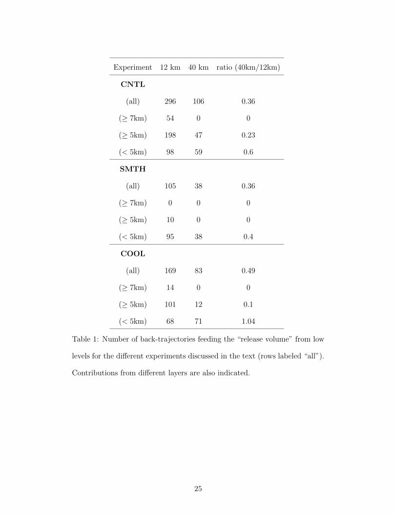
Table 1: Number of back-trajectories feeding the “release volume” from low

levels for the different experiments discussed in the text (rows labeled “all”).

Contributions from different layers are also indicated.

25

List of Figures537

1 Sea surface temperature (contoured every 2C) used in experi-538

ment (a) CNTL (b) SMTH and (c) COOL. Panel (d) gives the539

difference CNTL-SMTH (color) superimposed on the SST in540

panel (a). The SST in (a) is that observed on 14 January 2004,541

as given by the ECMWF operational analysis (25 km resolu-542

tion) and interpolated on the 12km grid of the MetUM model.543

The feature identified as the Gulf Stream “warm tongue” is544

highlighted in (a) in magenta. . . . . . . . . . . . . . . . . . . 29545

2 Snapshots at t = 24h of (a) vertical velocity (w, in m/s) at546

z = 5km and (b) equivalent potential temperature (θe, in K)547

at z = 500m. The corresponding surface temperature (=SST548

over the ocean) is shown in black with a contour interval of549

2C, starting from 0C (this is the SST distribution used in550

the CNTL experiment). The “white corners” indicate the limit551

of the nested 12km domain in that particular portion of the552

Northwest Atlantic. . . . . . . . . . . . . . . . . . . . . . . . . 30553

26

3 Back trajectories from the core of ascending motion at t =554

24h at midlevels (the “release volume” in black) in (a) the555

CNTL, (b) the SMTH and (c) the COOL experiments. The556

corresponding SST is shown in black with a contour interval557

of 2K. Note that only trajectories originating from low levels558

over the ocean at t=0h are shown while their highest location559

zi at t=24h is color coded (magenta for zi ≥ 7 km, green for560

5 km ≤ zi ≤ 7 km, blue for zi ≤ 5 km). . . . . . . . . . . . . . 31561

4 Meridional section at t = 24h of vertical velocity w (black562

contours, CI = 0.1m/s for upward motion in continuous,563

CI = 0.025m/s for downward motion in dashed, zero contour564

omitted) and equivalent potential temperature θe (white con-565

tours, CI = 10K) for (a) the CNTL and (b) the COOL exper-566

iment. Superimposed in both panel in colour is the difference567

in θe between CNTL and COOL. The meridional section was568

constructed by averaging gridpoints within the 66W − 69W569

longitude band. . . . . . . . . . . . . . . . . . . . . . . . . . . 32570

5 Schematic of ocean-atmosphere interactions associated with571

the warm sector of cyclones. The magenta curves are the572

same as those shown in Fig. 3a, i.e., backward trajectories573

located above 7 km at t = 24 h in the CNTL experiment574

(12km resolution) and reaching low levels over the ocean at575

t = 0h. The SST field for this experiment is also plotted in576

colours. . . . . . . . . . . . . . . . . . . . . . . . . . . . . . . 33577

27

6 PDFs of Lagrangian vertical velocity wL (in m/s) for the (a)578

CNTL (b) SMTH and (c) COOL experiments. In each panel,579

the 12km simulation is shown in grey and the 40km in dashed580

black. The PDFs were constructed using a width of 0.25 m/s.581

Note the log-scale on the vertical axis. . . . . . . . . . . . . . 34582

7 Fraction of the time in winter (in %) when the condition ∆θe >583

0 is met for a surface θe (a) equal to an equilibrium value584

(b) equal to the actual θe at 950hPa –see Section 3. The585

wintertime mean SST is displayed in black contours with a586

contour interval of 2C. All data from ERA-interim in boreal587

winter. Note the factor of four difference between the colorbars588

in (a) and (b). . . . . . . . . . . . . . . . . . . . . . . . . . . . 35589

8 Number of trajectories (circles) with heights z ≥ 5km at590

t=24h and reaching low levels over the ocean at t=0h (from591

Table 1 for all experiments): red for CNTL, blue for COOL592

and green for SMTH. The arrows indicate a measure of oceanic593

forcing when comparing CNTL/SMTH or CNTL/COOL (see594

main text). Note that the number of trajectories was normal-595

ized such that the number for CNTL at 12km resolution is596

unity in order to facilitate the comparison between experiments. 36597

28

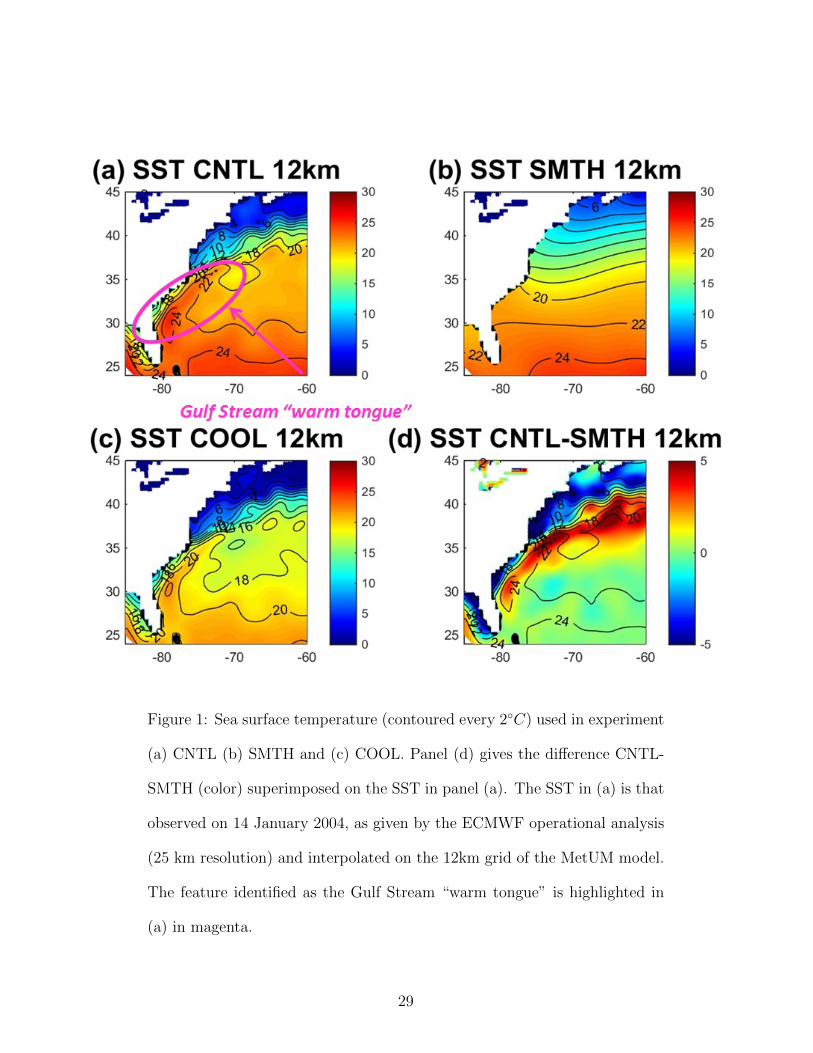
Figure 1: Sea surface temperature (contoured every 2C) used in experiment

(a) CNTL (b) SMTH and (c) COOL. Panel (d) gives the difference CNTL-

SMTH (color) superimposed on the SST in panel (a). The SST in (a) is that

observed on 14 January 2004, as given by the ECMWF operational analysis

(25 km resolution) and interpolated on the 12km grid of the MetUM model.

The feature identified as the Gulf Stream “warm tongue” is highlighted in

(a) in magenta.

29

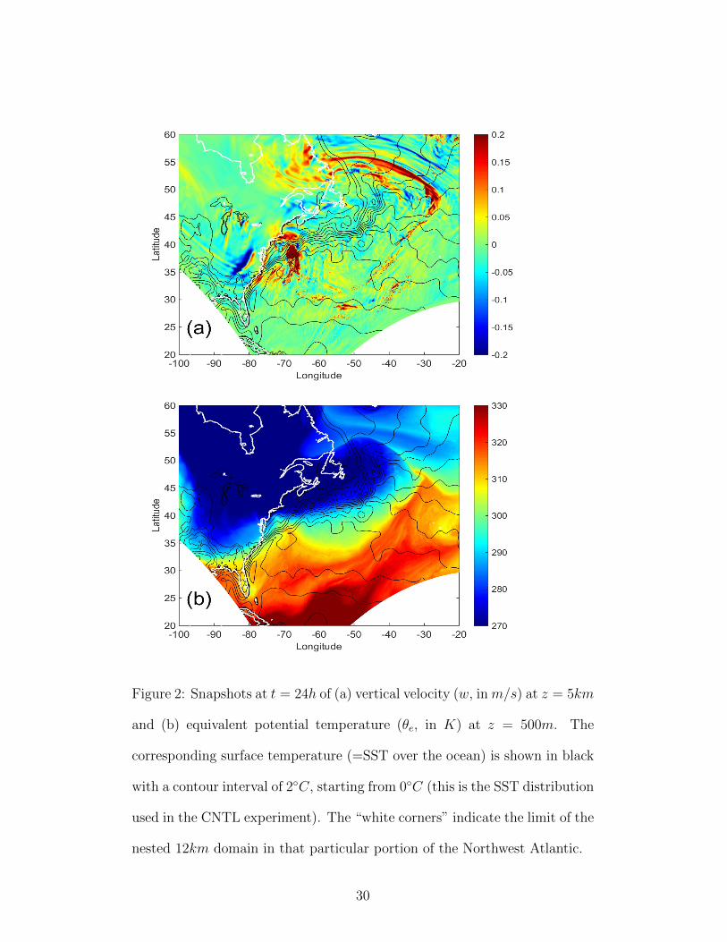
Figure 2: Snapshots at t = 24h of (a) vertical velocity (w, in m/s) at z = 5km

and (b) equivalent potential temperature (θe, in K) at z = 500m. The

corresponding surface temperature (=SST over the ocean) is shown in black

with a contour interval of 2C, starting from 0C (this is the SST distribution

used in the CNTL experiment). The “white corners” indicate the limit of the

nested 12km domain in that particular portion of the Northwest Atlantic.

30

Figure 3: Back trajectories from the core of ascending motion at t = 24h at

midlevels (the “release volume” in black) in (a) the CNTL, (b) the SMTH

and (c) the COOL experiments. The corresponding SST is shown in black

with a contour interval of 2K. Note that only trajectories originating from

low levels over the ocean at t=0h are shown while their highest location zi

at t=24h is color coded (magenta for zi ≥ 7 km, green for 5 km ≤ zi ≤ 7

km, blue for zi ≤ 5 km).

31

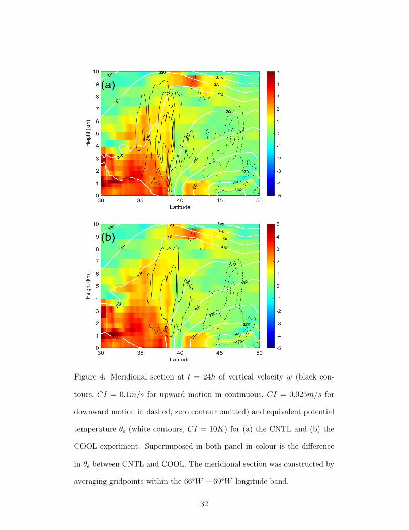
Figure 4: Meridional section at t = 24h of vertical velocity w (black con-

tours, CI = 0.1m/s for upward motion in continuous, CI = 0.025m/s for

downward motion in dashed, zero contour omitted) and equivalent potential

temperature θe (white contours, CI = 10K) for (a) the CNTL and (b) the

COOL experiment. Superimposed in both panel in colour is the difference

in θe between CNTL and COOL. The meridional section was constructed by

averaging gridpoints within the 66W − 69W longitude band.

32

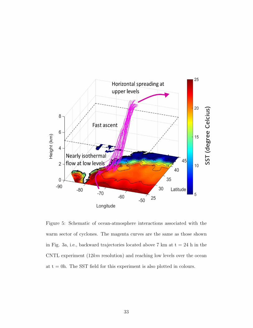
Figure 5: Schematic of ocean-atmosphere interactions associated with the

warm sector of cyclones. The magenta curves are the same as those shown

in Fig. 3a, i.e., backward trajectories located above 7 km at t = 24 h in the

CNTL experiment (12km resolution) and reaching low levels over the ocean

at t = 0h. The SST field for this experiment is also plotted in colours.

33

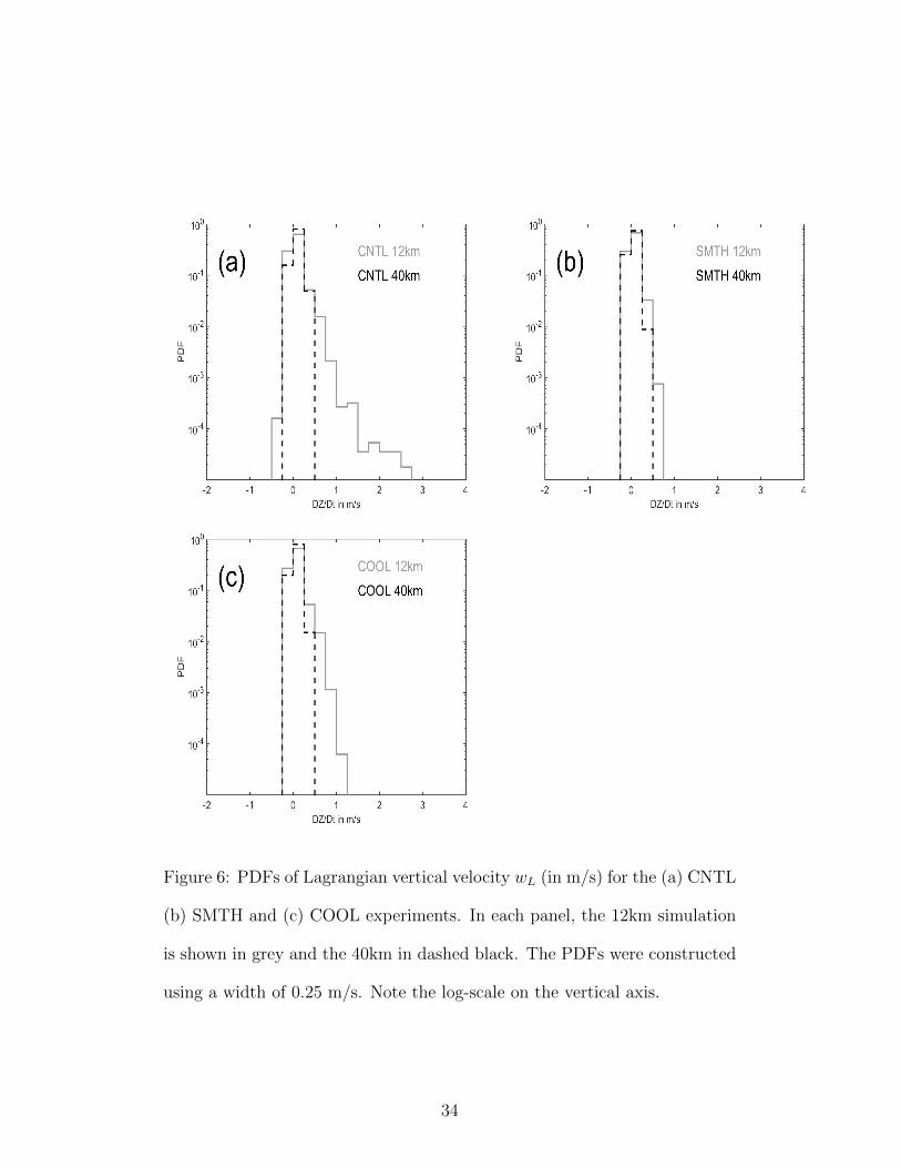
Figure 6: PDFs of Lagrangian vertical velocity wL (in m/s) for the (a) CNTL

(b) SMTH and (c) COOL experiments. In each panel, the 12km simulation

is shown in grey and the 40km in dashed black. The PDFs were constructed

using a width of 0.25 m/s. Note the log-scale on the vertical axis.

34

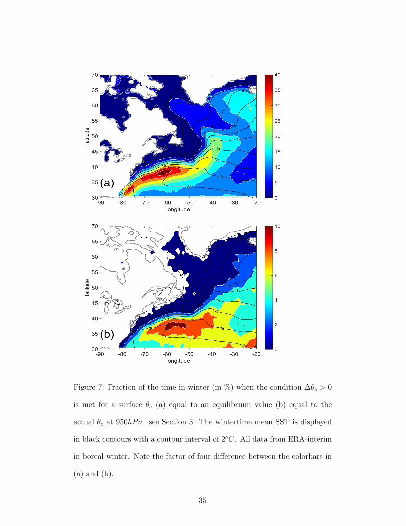
Figure 7: Fraction of the time in winter (in %) when the condition ∆θe > 0

is met for a surface θe (a) equal to an equilibrium value (b) equal to the

actual θe at 950hPa –see Section 3. The wintertime mean SST is displayed

in black contours with a contour interval of 2C. All data from ERA-interim

in boreal winter. Note the factor of four difference between the colorbars in

(a) and (b).

35

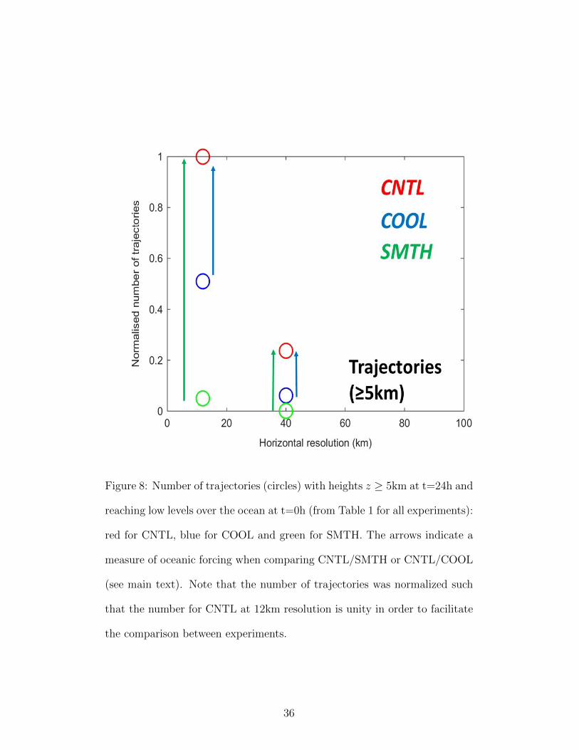
Figure 8: Number of trajectories (circles) with heights z ≥ 5km at t=24h and

reaching low levels over the ocean at t=0h (from Table 1 for all experiments):

red for CNTL, blue for COOL and green for SMTH. The arrows indicate a

measure of oceanic forcing when comparing CNTL/SMTH or CNTL/COOL

(see main text). Note that the number of trajectories was normalized such

that the number for CNTL at 12km resolution is unity in order to facilitate

the comparison between experiments.

36