wapor quality assessment
TRANSCRIPT

WaPOR quality assessment
WaPOR quality assessment
Technical report on the data quality of the WaPOR FAO database version 1.0
Technical report on the data quality of the WaPOR FAO database version 1.0This report describes the quality assessment of the FAO’s data portal to monitor Water Productivity through Open access of Remotely sensed derived data (WaPOR 1.0). The WaPOR 1.0 data portal has been prepared as a major output of the project: ´Using Remote Sensing in support of solutions to reduce agricultural water productivity gaps’, funded by the Government of The Netherlands. The WaPOR database is a comprehensive database that provides information on biomass production (for food production) and evapotranspiration (for water consumption) for Africa and the Near East in near real time covering the period 1 January 2009 to date. This report is the result of an independent quality assessment of the different datasets available in WaPOR prepared by IHE-Delft. The quality assessment checks the consistency of the different layers and compares the individual layers to various other independent data sources, including: spatial data; auxiliary data and in-situ data. The report describes the results of the quality assessment per data layer for each specific theme as available on the portal
CA4895EN/1/06.19
ISBN 978-92-5-131535-4
9 7 8 9 2 5 1 3 1 5 3 5 4
WaPOR quality assessm
ent - Technical report on the data quality of the WaPOR FAO database version 1.0
FAO - IHE Delft


WaPOR quality assessmentTechnical report on the data quality of the WaPOR FAO database version 1.0
Food and Agriculture Organization of the United NationsRome, 2019

Required citation: FAO and IHE Delft. 2019. WaPOR quality assessment. Technical report on the data quality of the WaPOR FAO database version 1.0. Rome. 134 pp.
The designations employed and the presentation of material in this information product do not imply the expression of any opinion whatsoever on the part of the Food and Agriculture Organization of the United Nations (FAO) or –IHE Delft Institute for Water Education (IHE DELFT) concerning the legal or development status of any country, territory, city or area or of its authorities, or concerning the delimitation of its frontiers or boundaries. The mention of specific companies or products of manufacturers, whether or not these have been patented, does not imply that these have been endorsed or recommended by FAO or IHE DELFT in preference to others of a similar nature that are not mentioned. The views expressed in this information product are those of the author(s) and do not necessarily reflect the views or policies of FAO or IHE DELFT.
FAO encourages the use, reproduction and dissemination of material in this information product. Except where otherwise indicated, material may be copied, downloaded and printed for private study, research and teaching purposes, or for use in non-commercial products or services, provided that appropriate acknowledgement of FAO and IHE DELFT as the source and copyright holders is given and that FAO/IHE DELFT's endorsement of users' views, products or services is not implied in any way.
All requests for translation and adaptation rights, and for resale and other commercial use rights should be made via www.fao.org/contact-us/licence-request or addressed to [email protected].
FAO information products are available on the FAO website (www.fao.org/publications) and can be purchased through [email protected]"
© FAO and IHE Delft, 2019
ISBN 978-92-5-131535-4

III
ContentsAcknowledgements X
AbbrevIAtIons And Acronyms XI
eXecutIve summAry XIII
1. IntroductIon 1
A. Overview 1
B. Quality Assessment 2
2. clImAte 5
A. Precipitation 5
B. Reference Evapotranspiration 8
3. wAter 13
A. Actual Evapotranspiration and Interception 13
B. Separation of Evaporation-Transpiration-Interception 38
C. Robustness 44
4. lAnd 51
A. Above Ground Biomass Production 51
B. Land cover classification 66
C. Phenology 72
5. wAter productIvIty 81
A. Gross Water Productivity 81
6. synthesIs 89
7. neXt steps 91
references 93
AnneX A: swAt model set-up 105
AnneX b: compArIson wApor AetI to other remote sensIng 108 AetI products usIng wAter bAlAnce At rIver bAsIn scAle
AnneX c: compArIson fluXnet vs wApor AetI 109

Iv
AnneX d: e, I And AetI compArIson etmonItor And wApor 110
AnneX e: wApor phenology stArt of croppIng seAson 115
AnneX f: proposed methodologIcAl Improvements 116 ArIsIng from the QA report
Figures1 Average annual WaPOR PCP (2009-2017) using two different legends 7
2 Average annual PCP Harvest Choice (HC) and difference between the HC 8 (1901-2005) and WaPOR data (2009-2017)
3 WaPOR Average Annual RET for the years 2009-2017 and difference 9 between average annual RET and RET 2009.
4 TerraClimate RET Comparison WaPOR RET and TerraClimate RET 10 (average for 2009-2017)
5 GLDAS RET and comparison with WaPOR RET for the year 2010 11
6 RET from Egypt Port Said Station and WaPOR RET for 2014 – 2015 12
7 RET station data and WaPOR RET data for Tal Amara, Lebanon 12
8 Average annual WaPOR AETI (2009-2017) 15
9 Comparison of the spatial distribution of AETI for 2010 from different products 17
10 TerraClimate AETI product compared to WaPOR AETI 18
11 GRDC stations in Africa and the spatially averaged AETI determined 19 from the water balance of the Congo, Niger and Nile basins
12 Comparison of WaPOR and WB AETI for 28 selected 20 river basins covering the period 2009 to 2017
13 Long-term annual average AETI estimates by 21 WaPOR (2009-2017) and SWAT+ (2010-2016) and difference between WaPOR and SWAT+ AETI for Africa
14 Discharge in Markaba tunnel after hydropower turbines at Abd el Al station 24
15 Longer-term trend of declining water storage in Lebanon 24 based on GRACE gravity measurements

v
16 Total discharge from Litani outlet at sea mouth and Markaba 25 tunnel compared with PCP – AETI – ΔS, based on remote sensing data
17 Geographical location of the sub-basins according to NBI 27
18 Relationship between the longer-term total FAO-Nile and 29 WaPOR AETI per sub-basin of the Nile
19 Location of the Fayoum Depression in Egypt. 30 The shape file indicates all irrigated areas
20 Comparison Fluxnet tower and WaPOR AETI 31
21 Comparison flux tower and WaPOR AETI in South Africa 32
22 Comparison flux tower AETI data and WaPOR AETI 32 at Cathedral Peak, South Africa
23 Temporal variability of flux measurements and 34 WaPOR AETI for the flux site Sakha-A
24 WaPOR T, E and I for the year 2010 38
25 WaPOR and ETMonitor comparison of annual T values 40
26 GLDAS T comparison with WaPOR T for the year 2010 41
27 Budyko T and comparison with WaPOR T 41
28 Location of the sap flow measurements in Tunisia 42
29 Measurement of actual transpiration fluxes with sapflow 43 devices in a grape plantation in northeastern Tunisia.
30 Average WaPOR AETI over RET (2009-2017), with 46 locations of selected irrigation schemes
31 Fraction of T over AETI (2009-2017) 47
32 The AETI/RET ratio and T/RET ratio for selected 48 irrigation schemes for year 2015
33 Monthly AETI/RET ratio for selected irrigation schemes 49
34 Monthly T/RET ratio for selected irrigation schemes 49
35 Annual Above Ground Biomass Production (AGBP) and Net Primary 53 Production (NPP) values averaged for 2009-2017 period
36 WaPOR NPP and average of MODIS Terra and Aqua NPP for 2011 54

vI
37 Difference NPP WaPOR and MODISAv as a fraction of MODISAv 54 and as absolute value for 2011
38 Global and annual NPP values simulated with the 55 IBIS model and difference with WaPOR NPP
39 WaPOR Above Ground Biomass Production for 57 2015 for the Wonji irrigation scheme
40 WaPOR derived yield for 2015 for the Wonji irrigation scheme 57 using AGBP and specific conversion factors for sugarcane
41 Sugarcane yield distribution Wonji irrigation scheme 58
42 WaPOR AGBP for Bekaa Valley for the year 2015 59
43 Yield distribution of grapes in Bekaa Valley for the year 2015 60
44 WaPOR AGBP at Kpong irrigation scheme for the year 2015 60
45 WaPOR yield estimation for banana plantation at 61 Kpong irrigation scheme for the year 2015
46 Distribution of WaPOR estimated yield for Kpong 62 irrigation scheme for the year 2015
47 WaPOR AGBP for the year 2015 63
48 WaPOR derived yield for wheat (November 2015- May 2016) 64 and maize (June-October 2016)
49 WaPOR yield distribution for wheat, maize and 65 oranges in Fayoum irrigation scheme for the year 2015
50 Comparisons of rainfed and irrigated areas in 68 18 countries from WaPOR, GMIA, and GIAM
51 Comparison of WaPOR LCC with WA+ LCC in Jordan and 69 Awash and local database (Litani)
52 WaPOR phenology for selected 100 m countries expressed 72 in terms of the start of season 1 and 2 in 2015
53 Start of cropping season in Ghana 73
54 Start of season 1 and length of season at Kpong irrigation for 2015 75
55 Start of season 1 and length of season at Fayoum irrigation scheme for 2015 76
56 Start of season 1 and length of season at Wonji irrigation for 2015 77

vII
57 Start of growing season 1 and length of growing season Bekaa Valley 78
58 Season 1 and season 2 pixel identification 79
59 Average WaPOR gross biomass WP (GBWP) and net biomass WP 82 (NBWP) for 2009-2017.
60 Servir WP and difference between Servir and WaPOR WP (2009-2013) 83
61 Gross WP for Wonji (30 m resolution) 84
62 Gross Water Productivity wheat and maize 85
63 Kpong gross WP rice season 1 and season 2 86
64 Kpong gross WP bananas 87
Tables1 Thematic areas and WaPOR data components available 2 for different spatial resolutions
2 Overview of comparisons made for each layer 3
3 Example of available real time PCP data products over Africa 6
4 Average annual WaPOR PCP statistics for the African continent 7
5 Mean annual WaPOR RET and standard deviations (for all regions) 9
6 WaPOR AETI 2009-2017 14
7 Example of available remote sensing products of AETI over Africa 16
8 Statistics of AETI products over Africa 2010 17
9 Comparison of various AETI products for the 28 river basins 20 specified in Figure 12
10 Comparison of AETI estimates using PCP-Q, WAPOR and SWAT+ 22 for basins in Africa
11 Comparison of annual P and ET values for the entire 25 Litani Basin based on the original WaPOR data.
12 Average annual water balance components of the 25 Litani River Basin using WaPOR data inputs

vIII
13 Comparison of AETI estimates using the water balance, 26 WaPOR and past studies in the Nile Basin
14 AETI statistics per sub-basin according to FAO-Nile and WaPOR 28
15 Annual AETI of the land use class irrigated land in Fayoum Depression 29
16 Comparison of annual WaPOR and measured AETI on 33 traditionally irrigated crops in the Nile Delta
17 Seasonal measured and WaPOR AETI fluxes 35
18 Components of the field scale soil water balance in irrigated 36 vegetables in the Jordan Valley; the Jordan component
19 Components of the field scale soil water balance in irrigated vegetables in the Jordan Valley ; the Israel component 36
20 Synthesis of in situ comparison of WaPOR AETI data 37
21 Overview of continental values of WaPOR AETI, T, E and 39 I per land use class in mm/yr for year 2010
22 Overview of continental values of AETI, T, E and I for four 39 different spatial products in mm/yr for year 2010
23 Light extinction factor for net radiation 44
24 Overview of continental values of WaPOR robustness 46
25 Overview of WaPOR AETI, T, E and I per selected irrigation scheme for 2015 47
26 Average continental values of WaPOR ABGP and NPP 53
27 WaPOR yield estimates for Kpong irrigation scheme for the year 2015 58
28 WaPOR yield for grapes in Bekaa Valley for the year 2015 59
29 WaPOR yield estimates for Kpong irrigation scheme for the year 2015 61
30 Crop productivity Fayoum system 64
31 Rainfed and irrigated areas from WaPOR (2014), 67 FAO AQUASTAT (2013-7) and GIAM (2010)
32 The comparisons of WaPOR LCC map with that from 70 RCMRD and RWFA for Rwanda.
33 Confusion matrix of WaPOR land cover map of Ethiopia for year 2014 71
34 Confusion matrix for WaPOR 2009 land cover map in Benin 71

IX
35 Cropping season in Kpong irrigation scheme 74
36 WaPOR phenology indicators for Kpong irrigation scheme in 2015 74 (mean and standard deviation)
37 Cropping season in Fayoum irrigation scheme 76
38 WaPOR phenology indicators for Fayoum irrigation scheme in 2015 76 (mean and standard deviation)
39 WaPOR phenology indicators for Wonji irrigation scheme in 2015 77 (mean and standard deviation)
40 Cropping season of potatoes in Bekaa Valley irrigation 77
41 WaPOR phenology indicators for Bekaa Valley irrigation in 2015 78 (mean and standard deviation)
42 Key indicators for Water Productivity in Wonji irrigation scheme 84
43 Key indicators for Water Productivity in Fayoum irrigation scheme 85
44 Key indicators for Water Productivity in Kpong irrigation scheme 86

X
AcknowledgementsThis report was prepared by Marloes Mul and Wim Bastiaanssen, with contributions from: Jonna van Opstal,
Xueliang Cai, Ann van Griensven, Imeshi Weerasinghe, Bich Tran, Tim Hessels, Bert Coerver, Claire Michailovsky,
Elga Salvadore, Ate Poortinga, Poolad Karimi, and Li Jia.
The FAO Land and Water Division commissioned this study and provided layout and editorial work in the
framework of the the project ´Using Remote Sensing in support of solutions to reduce agricultural water
productivity gaps`, funded by the Government of The Netherlands. The work was carried out by a team in
IHE-Delft as an independent quality assessment of the WaPOR database and, as such, the views expressed in the
report are those of the authors.
The report contains various type of analysis and quality checks. Most of the data has been assembled during
the last two years. During the writing of the report, new global datasets became available. Some of them are
included – or could be included in a future version of this report. It is the intention of the authors to include more
ground measurements collected by IHE Delft students for the current and next academic year and intensify the
exchanges with the various international partners in Africa and Near East. The continuation of quality control
can benefit from the strengths and weaknesses found in the current report. Validation of the rich database of
WaPOR with unprecedented possibilities is an evolving effort.
The essence of this validation report is to collect independent datasets and make comparative analysis. While
most spatial data layers can be accessed through the public domain (although not all), the real value comes from
the data sharing of third parties. We are therefore indebted to many international partners. We thank the team
at Global Runoff Data Centre (GRDC), 56 068 Koblenz, Germany for providing the discharge data. We acknowl-
edge the sharing of sap flow field measurements conducted by Karim Bergaoui and Makhram Belhaj Fraj from
Tunisia. Michael Gilmont from the University of Oxford kindly made his field measurements from Jordan and
Israel available. Jiro Ariyama from the FAO office in Cairo kindly assisted in the flux analysis of the eddy covari-
ance towers in the Nile Delta of Egypt. Caren Jarmain, Colin Everson, Alistair Clulow and Graham Jewitt from
the University of Kwazulu Natal provided flux tower data from South Africa, including the Cathedral Peak data
from the South African Environmental Observation Network (SEAON), and the Lebanese Agricultural Research
Institute (LARI) made the weather data available for the Bekaa Valley, and the Wonji Shoa Research Centre and
factory made the yield data available in the Wonji irrigation scheme. Finally, the Ministry of Water Resources and
Irrigation of Egypt provided data for the Fayoum irrigation scheme.
Some spatial maps were provided for making extra analysis feasible. For example, AETI data products were made
available by various people and we are grateful for their support, this includes Li Jia for making the ETMonitor
data available, Albert van Dijk for the CMRSET and Xuelong for the SEBS data, Seyed Hamed Alemohammad
for the WECANN data and Martha Anderson for the ALEXI data. The National Council for Scientific Research
of Lebanon is acknowledged for sharing the land use map of the Litani Basin. The Water for Growth Rwanda
(W4GR) project kindly made their land use map available. The team of Miriam Coenders–Gerrits at TUDelft
shared with us the newest T and I maps following their Budyko methodology. The SERVIR Mekong team kindly
made code available for global WP analysis on the Earth Engine.

XI
Abbreviations and AcronymsAETI Actual Evapotranspiration and Interception
AGBP Above Ground Biomass Production
ALEXI Atmosphere Land Exchange Inverse (model)
ARC African Rainfall Climatology
CHIRPS Climate Hazards Group InfraRed Precipitation with Stations
CMORPH Climate Prediction Center’s morphing technique
CMRSET CSIRO MODIS ReScaled potential ET
CNRS National Council for Scientific Research (Lebanon)
CRU Climatic Research Unit
DEM Digital Elevation Model
DM Dry Matter
E Evaporation (from soil)
ETLook EvapoTranspiration Look (model)
EWEMBI EartH2Observe observations, WFDEI and ERA-Interim data Merged and Bias-corrected for ISIMIP
FAO Food and Agricultural Organization of the United Nations
FLUXNET Flux Network for in situ measurements of turbulent fluxes (H20, CO2, heat)
FRAME FAO Remote sensing Assessment for Monitoring and Evaluation (Consortium)
GBWP Gross Biomass Water Productivity
GIAM Global Irrigated Area Map
GMIA Global Map of Irrigated Areas
GLDAS Global Land Data Assimilation System
GLEAM Global Land surface Evaporation: the Amsterdam Methodology
GOES-5 Geostationary Operational Environmental Satellite system
GRDC Global Runoff Data Centre
GT Ground truth
HC Harvest Choice
I Interception
ITC International Institute for Geo-Information Science and Earth Observation
ITCZ Inter Tropical Convergence Zone
IWMI International Water Management Institute
LAI Leaf Area Index

XII
LandFluxEval Land Flux Evaluation data base
LCC Land Cover Classification
LRA Litani River Authority
MENA Middle East and Northern Africa
MERRA Modern-Era Retrospective Analysis for Research and Applications
MODIS MODerate resolution Imaging Spectroradiometer
MSG Meteosat Second Generation
MTE Model Tree Ensemble
NBWP Net Biomass Water Productivity
NDVI Normalized Difference Vegetation Index
NPP Net Primary Production
PCP Precipitation
PERSIANN-CDR Precipitation Estimation from Remotely Sensed Information using Artificial Neural Networks
RCMRD Regional Centre for Mapping of Resources for Development
RET Reference Evapotranspiration
RFE African Rainfall Estimation
RWFA Rwanda Water and Forestry Authority
SEBS Surface Energy Balance System
SERVIR-Mekong geospatial data-for-development program for the Lower Mekong SSEBop Operational Simplified Surface Energy Balance
SWAT+ Soil and Water Assessment Tool
T Transpiration
TAMSAT Tropical Applications of Meteorology using SATellite
TBP Total Biomass Production
TC TerraClimate
TE Transpiration Efficiency
TRMM Tropical Rainfall Measuring Mission
USGS United States Geological Survey
VITO Flemish Institute for Technological Research
WA+ Water Accounting plus
WACMOS-ET WAter Cycle Observation Multi-mission Strategy - EvapoTranspiration
WaPOR FAO portal to monitor Water Productivity through Open access of Remotely sensed derived data
WB Water Balance
WECANN Water, Energy, and Carbon with Artificial Neural Networks
WP Water Productivity

XIII
Executive summary This report describes the quality assessment of the FAO’s data portal to monitor Water Productivity through Open
access of Remotely sensed derived data (WaPOR 1.0). The WaPOR 1.0 data portal has been prepared as a major
output of the project: ́ Using Remote Sensing in support of solutions to reduce agricultural water productivity gaps’,
funded by the Government of The Netherlands. The WaPOR database is a comprehensive database that provides
information on biomass production (for food production) and evapotranspiration (for water consumption) for
Africa and the Near East in near real time covering the period 1 January 2009 to date. This report is the result of an
independent quality assessment of the different datasets available in WaPOR prepared by IHE-Delft. The quality
assessment checks the consistency of the different layers and compares the individual layers to various other
independent data sources, including: spatial data; auxiliary data and in-situ data. The report describes the results of
the quality assessment per data layer for each specific theme as available on the portal:
Precipitation (PCP)The PCP dataset posted on the WaPOR data portal is a copy of CHIRPS, with a few modifications for data gaps
in agricultural areas. This dataset has been validated by different independent and international science teams.
The CHIRPS database is among the top PCP databases available online and performs specifically well on decadal
timescales.
Reference Evapotranspiration (RET)The WaPOR RET data is able to correctly express RET climatic evapotranspiration across the continent. On the
continental level, variations in RET between years are low (varying less than 25 mm per year, 0.6%). A similar trend
is also observed for one weather station. The WaPOR RET data is able to identify the impacts of 2009 El Nino event,
with higher than average RET in Southern and West Africa and lower RET values in East Africa, consistent with El
Nino anomalies. However, some more validation with ground-based weather station data remains necessary.
Actual Evapotranspiration and Interception (AETI)Compared to similar remote sensing databases of actual evapotranspiration, WaPOR AETI is reliable for a longer
period (e.g. a year) and larger areas (e.g. a sub-basin). The annual AETI for Litani basin in Lebanon is excellent. The
quality reduces with a higher aridity such as in Egypt and South Africa. The 250m and 100m pixels are less suitable
for detecting AETI of vegetables and fruit crops; 30 m pixels add a lot of value. However there are several challenges
with the breakdowns of annual AETI into monthly and decadal values, and also spatially for local agricultural fields.
The latter is manifested in the validation with individual flux tower data (eddy covariance and surface renewal).
WaPOR AETI for the crop season is systematically underestimated (20-60%). Hence, a spatial and temporal
refinement of AETI is required. It is fair to note that field measurements on AETI often have their own uncertainties.
Transpiration, Evaporation, Interception (T, E, I)All three products individually showed reasonable ranges in values and spatial variability. Compared to ETMonitor,
WaPOR T estimates are high and WaPOR E estimates are low. The high WaPOR ratio of T/AETI is consistent with
the Budyko approach, exceeding at the continental scale 0.7 ratio. While this does not always match with the general

XIv
opinion, 0.7 ratio and higher for tropical forest and permanent crops are very acceptable. For the selected irrigation
systems in Ethiopia, Egypt, Lebanon and Ghana similar high T/AETI are found (>0.73), consistent for vegetated
areas.
Above Ground Biomass Production (AGBP)Agro-ecological production is commonly expressed as Net Primary Production (NPP) in remote sensing
terminology, or crop yield in agronomic terms. A direct comparison against AGBP from other sources is difficult.
The comparison against NPP from MODIS and global ecological production models does not identify serious
problems at the continental scale: the absolute values and aerial patterns of NPP are very acceptable. This is
confirmed from the crop yield analysis for sugarcane (Ethiopia), grapes (Lebanon), rice and bananas (Ghana) and
wheat (Egypt). Fresh crop yield could be very well approximated, provided that local calibration of Harvest Index
and the moisture content of the harvestable product is considered and the cropping season is defined on the basis
of local information. This implies that local agronomical knowledge is necessary to convert AGBP into crop yield.
Some warning on the role of the default 0.65 shoot-root ratio and default C3 crop maximum light use efficiency of
2.49 gr/MJ of total dry matter for all C3 and C4 crops should be mentioned in the information section of the WaPOR
website.
Land cover classificationLand cover classification, as all data layers, has been created with different spatial resolutions. The single most
relevant class for water productivity is the distinction between rainfed and irrigated crops. While the WaPOR
irrigated area extent is at times comparable to the GMIA from FAO AQUASTAT, verification with other sources and
field measurements indicated that a serious underestimation occurs. The procedure applied for mapping irrigated
areas may need to be improved.
PhenologyThe crop phenology is essential for assessing the accumulated values of biomass production (AGBP and TBP) and
water consumption (AETI). This study finds that the accuracy of the phenology is poor and does not match with
local cropping calendars. This is a serious limitation for approximating the accumulated values between dates
of emergence and date of harvest. This part of WaPOR can currently not be used without local information or
validation, and an appropriate warning should be provided through the WaPOR portal.
Water productivityThe water productivity layer in WaPOR is a compilation of other WaPOR layers (phenology, land use, AGBP, AETI
and T), errors in those layers are therefore compounded in the water productivity layer. The errors in the phenology
and land cover classification layers were overcome by applying the start and end date of the season and using a
polygon of the field obtained from observations. The analyses show very good comparisons with a slight deviation
due to the inclusion of fallow land within the polygons. For example the WP analyses for sugarcane (Ethiopia)
is therefore underestimated with non farm land (fallow land, buildings, roads and open water) showing low WP.
On the other hand, WP for wheat and maize (Egypt) can be overestimated as included fallow areas show high WP.
Finally, WP analyses in a humid zone (Southern Ghana) shows little distinction between the agricultural lands and
the surrounding natural vegetation. It is clear that detailed cropping maps are required to exclude this kind of noise
from the WP analyses.

Det
ail o
f WaP
OR
Map
“G
ross
Bio
mas
s W
ater
Pro
duct
ivit
y 20
18 -
Ken
ya, S
omal
ia a
nd E
thio
pia”
1. Introduction
A. overviewThis report is an output of the project “Using Remote Sensing in support of solutions to reduce agricultural water
productivity gaps”, funded by the Government of The Netherlands. The project is lead by FAO with the following
project partners: FRAME consortium, IHE Delft and IWMI. The objective of the project is monitoring water
productivity, identifying water productivity gaps, proposing solutions to reduce these gaps and contributing
to a sustainable increase of agricultural production. The main output is to develop an open access data portal
on remotely sensed derived water productivity in Africa and the MENA region, hosted by FAO. The FRAME
consortium, consisting of eLEAF, VITO, ITC, and the WaterWatch Foundation, is responsible for creating and
providing the remote sensing data for the project. In April 2017, FAO’s portal to monitor Water Productivity through
Open access of Remotely sensed derived data (WaPOR) was launched as a Beta version. Two parallel independent
quality assessments of the Beta version were implemented by IHE Delft and ITC. Recommendations from these
assessments were used to prioritize improvements for WaPOR version 1.0. In August 2018, this improved version
was made available through the link: https://wapor.apps.fao.org (version 1.0), in December 2018 some additional
improvements on the user interface of the portal were made available through version 1.1. An overview of the
available WaPOR data is provided in Table 1.

2 WaPOR quality assessment
The WaPOR database is the first comprehensive dataset that combines biomass production (for food production)
and AETI information (for water consumption) at continental scale near real time covering the period 1 January
2009 to date. It should be emphasized that the Gross WP and Net WP are based on Above Ground Biomass
Production and not on the fresh crop yield as is often done for international WP studies. The reason for avoiding
crop dependent information is the lack of accuracy to determine crop layers from earth observation data. The
validation of AGBP and WP can however only be done through conversion into crop yield data, because AGBP is
rarely measured under actual field conditions.
B. Quality AssessmentOutput 2 of the project includes a quality assessment of the WaPOR database. Results of this independent
assessment by IHE Delft are presented in this report. It is meant for an independent verification of WaPOR version
1.0 data and it forms a basis for including improvements in WaPOR version 2.0. This quality assessment checks the
consistency of the different layers and compares the individual layers to various products:
Table 1 Thematic areas and WaPOR data components available for different spatial resolutions*
Thematic area Layers Level 1 (250 m) Level 2 (100 m) Level 3 (30 m)
Climate Precipitation (PCP) Daily/decadal/annual (5km)
Reference Evapotranspiration (RET)
Daily/decadal/annual (20km)
Water Actual Evapotranspiration and Interception (AETI)
Decadal/annual Decadal/ seasonal/ annual
Decadal/ seasonal/ annual
Transpiration (T)
Evaporation (E)
Interception (I)
Land Above ground biomass production (AGBP)
Annual Decadal/ seasonal Decadal/ seasonal
Land cover classification (LCC)
Annual Annual Decadal
Phenology Seasonal Seasonal
Net Primary Production (NPP)
Decadal Decadal Decadal
Water Productivity (WP)
Gross WP Annual Seasonal Seasonal
Net WP Annual Seasonal Seasonal
* currently available products in the WaPOR portal

31. Introduction
- Spatial data products
- Auxiliary data comparison
- In-situ data comparison
Table 2 presents an overview of the comparisons made between the WaPOR database and other data sources.
Consistency checkFor each layer the general spatial trend is analysed, as well as the range of values in the layer. This is implemented
at continental level (WaPOR Level 1, 250 m resolution). The authors used their expert judgement to evaluate if the
values are in reasonable ranges.
Table 2 Overview of comparisons made for each layer
Thematic area
Layers Spatial data Auxiliary data In situ observations
Climate PCP CRU
RET GLDAS, TerraClimate Weather station data (Bekaa and Port Said)
Water AETI Various remote sensing data products, SWAT modelling output
Water balance for large river basins in Africa, Litani River Basin, Nile sub-basins, Fayoum irrigation scheme, field scale soil water (Jordan, Israel)
Flux towers (South Africa, Ghana, Senegal, Egypt)
T Remote sensing data products (ETMonitor, GLDAS), Budyko approach
Sap flow Tunisia
E
I
Land AGBP Remote sensing products (MODIS)
Comparisons with known yields (Wonji, Fayoum, Kpong, Bekaa Valley irrigation scheme)
LCC Other databases (GMIA, GIAM)
National statistics Rwanda GIAM Ground truth data points for Benin, Ethiopia
Phenology FAO crop calendarsa , case study information (Wonji, Fayoum, Kpong, Bekaa)
WP Gross WP WP MODIS & Servir Mekong
Case study data (Wonji, Fayoum, Bekaa)
Net WP
a http://www.fao.org/agriculture/seed/cropcalendar/welcome.do

4 WaPOR quality assessment
Spatial data Next to the WAPOR data, there are many other spatial data products available that monitor various WaPOR param-
eters. These spatial data products are either derived from remote sensing, similarly to WaPOR, or derived through
other means (e.g. modelling). The products were compared on their general trends and statistical properties and
differences with the WaPOR data were calculated and analysed. These analyses were done at continental level using
the WaPOR Level 1 data (250 m resolution).
Auxiliary data Several WaPOR layer products can be compared indirectly with auxiliary and independently gathered datasets. One
such example is the water balance calculations, which derives actual ET using observed data for a specific area. The
advantage of this method is that it integrates parameters over a specific area using observed and often validated
datasets. Depending on the scale of the analyses, the WaPOR data with the highest available resolution was used.
In situ observationsWhere possible, the WaPOR data layers are compared with in situ observations. As the WaPOR data has very high
resolution (250 m to 30 m on selected pilot areas), it is possible to validate the product using point observations.
This comparison has the highest value as it compares the same parameter using observed data. Depending on the
location of the in situ observation, the WaPOR data with the highest resolution was used for the comparison.
Robustness analysesFinally, the analyses focus on the consistency between the different WaPOR layers, in particular those that are
independently developed.
The selection of data for comparison and robustness analyses were dependent on the availability of data products
online and on willingness of our partners to share their data.
As can be seen from Table 2, the report provides a wide range of analyses to validate the WaPOR dataset. It combines
comparative analyses at continental level, various analyses at country, basin and field scale to the highest resolution
of comparison at pixel resolution. The report provides a first indication of the quality of the individual data layers.
The following chapters will describe the results of the quality assessment in three different thematic areas, similar
to the portal: climate, water, and land. Each chapter will contain an assessment of the data layers found in the
specific theme (Table 1).

51. Introduction
Det
ail o
f WaP
OR
Map
“A
ctua
l Eva
poT
rans
pira
tion
and
Inte
rcep
tion
(E
TIa
) 20
18 -
Dem
ocra
tic
Rep
ublic
of t
he C
ongo
, Tan
zani
a an
d Z
ambi
a”
2. Climate
A. precipitationA.1 IntroductionThere are various remote sensing products of precipitation (PCP) available in the open domain and in near-real-
time for Africa (Table 3). Some started in the 1980s and are continuing into the present. Increasingly remote sensing
data products have included bias-corrections using ground observations (e.g. Xie et al., 2011). Various studies
evaluated the performance of satellite-derived products. At continental scale, Awange et al. (2016) found that the
various products performed better at different time scales and different geographical locations. There is not one
product which outperforms the other products across temporal and spatial scales, although TRMM and CHIRPS
are often found to be among the more reliable products (e.g. Cheema and Bastiaanssen, 2011; Simons et al., 20016;
Ha et al., 2018). Generally, satellite remote sensing products that correct biases using ground observation performed
better compared to those that use remote sensing alone (Awange et al., 2016; Pomeon et al., 2017).
The CHIRPS dataset, used for the WaPOR database, is an existing data product and has a spatial resolution of 5
km (Funk et al., 2015). This database was modified for data gaps for WaPOR important agricultural areas (FAO,

6 WaPOR quality assessment
2018). The dataset combines remote sensing information with ground observations. In various studies, CHIRPS
data has been compared to observed PCP and other similar satellite PCP products. For example, in Burkina Faso,
daily products generally performed poorly compared to ground observations. Aggregated products at monthly
and annual scale performed much better (>0.8) (Dembele and Zwart, 2016). Data with higher spatial resolution
performed better at station to pixel level (Dembele and Zwart, 2016). For decadal scale, Dembele and Zwart (2016)
found that RFE performed best, closely followed by ARC and CHIRPS. Similarly, Hessels (2015) compared various
remotely sensed PCP products with weather station data from the Blue Nile region and found that the CHIRPS
data product displays the best correlation with station data. For East Africa, Dinku et al (2018) found that CHIRPS
performed better than ARC and slightly better than TAMSAT at decadal and monthly timescales (whereas TAMSAT
performed better at daily time scales).
A.2. Data analysesThe average annual PCP for the African continent lies between 537 and 597 mm per year (Table 4). The standard
deviation of the mean annual PCP is 18 mm per year, which shows at a continental scale a relatively constant annual
PCP. However, locally large variations in PCP occur between years with far reaching consequences for rainfed
cropping systems and flood risks. A few areas in the vicinity of steep mountain ranges show very high annual PCP
amounts (>3 000 mm per year) throughout the entire period. This is around the coast of West Africa and Cameroon
and the east coast of Madagascar (which are more visible when adjusting the legend) (Figure 1; right). The general
spatial variation in PCP at the continental scale is consistent with known PCP trends, low values are found across
the Sahel and the Middle East region. Also high amounts of PCP occur around the West Coast of Africa, around
the equator and the inlands of the Democratic Republic of Congo and highlands in East Africa (Uganda, Rwanda,
Ethiopia) and the east coast of Madagascar (Figure 1).
Table 3 Example of available real time PCP data products over Africa
Satellite product Temporal coverage
Spatial coverage
Spatial resolution
Temporal resolution
Reference
ARC Version 2.0 1983–present Africa 0.1° (~10 km) Daily Xie and Arkin, 1995
CHIRPS Version 2.0
1981–present Near global 0.05° (~5 km) Daily Funk et al., 2015
CMORPH 1998-present Africa 0.1° (~10 km) 3-hourly Joyce et al., 2004; Xie et al., 2011
PERSIANN-CDR 1983–present Near global 0.25°(~27 km) Daily Hsu et al., 1997; Novella and Thiaw, 2013, 2010
RFE Version 2.0 2001–present Africa 0.1° (~10 km) Daily Herman et al., 1997
TAMSAT 1983–present Africa 0.0375° (~4 km) Decal Maidment et al., 2014; Tarnavsky et al., 2014
TRMM 3B42 version 7
1998–present Near global 0.25°(~27 km) 3-hourly Maidment et al., 2014

72. Climate
Table 4 Average annual WaPOR PCP statistics (mm/yr) for the African continent
2009 2010 2011 2012 2013 2014 2015 2016 2017 Average
Min 0 0 0 0 0 0 0 0 0 0
Max 4 789 5 257 4 787 4 576 4 330 5 004 4 735 4 759 5 876 4 901
Mean 572 597 587 590 566 565 537 562 584 573
Sd 603 632 624 621 611 599 580 597 626 604
Comparison with other spatial data products
A comparison was made between the average annual PCP of Harvest Choice (HC) (Harvest Choice, 2011) and the
average annual precipitation of the WaPOR database (Figure 2). The HC dataset is based on the reanalysis dataset
from the University of East Anglia Climatic Research Unit (CRU) that essentially is interpolating and extrapolating
between measured rainfall at gauges (New et al., 2000). This dataset shows similar high PCP areas in West Africa
and Madagascar (Figure 2 left). Considering the difference in the period of observation (1901-2005 vs 2009-2017),
the general trend of PCP is similar between the two datasets, except for a few areas (Figure 2 right). These areas
were found in Madagascar and Eastern part of the Democratic Republic of Congo. We have more trust in the
CHIRPS data because many locations in Africa are not equipped with a rain gauge, and this affects the quality of the
CRU-based PCP dataset.
Figure 1 Average annual WaPOR PCP (2009-2017) using two different legends (based on quartiles, left and based on equal intervals, right).
wapor pcp (mm/yr)07531510003500
wapor pcp (mm/yr)0750150022503000

8 WaPOR quality assessment
A.3 ConclusionThe PCP dataset posted on the WaPOR data portal is based on the CHIRPS dataset. This dataset from USGS has
been validated and tested for many years by different independent science teams. The CHIRPS dataset is among
the top PCP products available online and performs specifically well on decadal timescales as shown by Dembele
and Zwart (2016).
b. reference evapotranspirationB.1. IntroductionAfter the introduction by FAO of the global standard Reference evapotranspiration (RET) (Allen et al., 1998), RET
became a well-recognized concept to express the climatologic variability of crop ET. The attractive character of RET
is that it is only affected by climatic factors, excluding other factors like for example crop and soil typology (Allen et
al., 1998). Over the past decades various approaches have been developed to calculate RET, often based on simpler
input data (e.g. Hargreaves and Samani, 1985; de Bruin et al., 2016). However, the Penman-Monteith equation (Allen
et al., 1998) is the most applied approach, after it was selected to be the best performing equation in a variety of
climates by an FAO expert consultation in 1990. The drawback is that more detailed climatological information is
required (radiation, humidity, temperature and wind speed), which is not always everywhere available in weather
stations over the African continent.
Solar radiation is nowadays available with an unprecedented accuracy from Second Generation Meteosat (MSG)
measurements over Africa and Near East. What remains is local prevailing humidity, temperature and wind speed,
that are more commonly taken from numerical climatic and weather forecasting models to fill the voids of in situ
Figure 2 Average annual PCP Harvest Choice (HC) and difference between the HC (1901-2005) and WaPOR data (2009-2017)
hc pcp (mm/yr) wapor- hc pcp (mm/yr)0750150022503000
-1500-75007501500
92. Climate
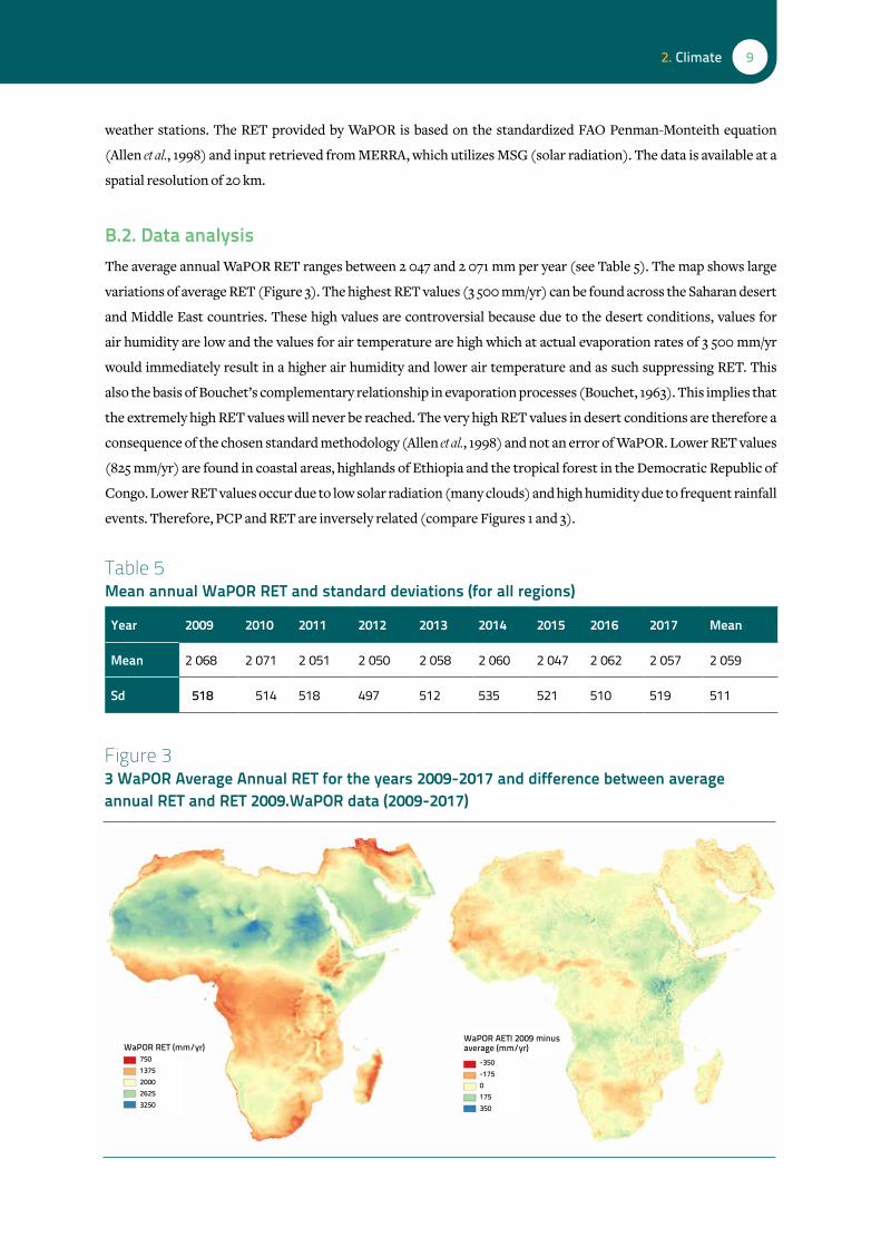
Figure 3 3 WaPOR Average Annual RET for the years 2009-2017 and difference between average annual RET and RET 2009.WaPOR data (2009-2017)
weather stations. The RET provided by WaPOR is based on the standardized FAO Penman-Monteith equation
(Allen et al., 1998) and input retrieved from MERRA, which utilizes MSG (solar radiation). The data is available at a
spatial resolution of 20 km.
B.2. Data analysisThe average annual WaPOR RET ranges between 2 047 and 2 071 mm per year (see Table 5). The map shows large
variations of average RET (Figure 3). The highest RET values (3 500 mm/yr) can be found across the Saharan desert
and Middle East countries. These high values are controversial because due to the desert conditions, values for
air humidity are low and the values for air temperature are high which at actual evaporation rates of 3 500 mm/yr
would immediately result in a higher air humidity and lower air temperature and as such suppressing RET. This
also the basis of Bouchet’s complementary relationship in evaporation processes (Bouchet, 1963). This implies that
the extremely high RET values will never be reached. The very high RET values in desert conditions are therefore a
consequence of the chosen standard methodology (Allen et al., 1998) and not an error of WaPOR. Lower RET values
(825 mm/yr) are found in coastal areas, highlands of Ethiopia and the tropical forest in the Democratic Republic of
Congo. Lower RET values occur due to low solar radiation (many clouds) and high humidity due to frequent rainfall
events. Therefore, PCP and RET are inversely related (compare Figures 1 and 3).
Table 5 Mean annual WaPOR RET and standard deviations (for all regions)
Year 2009 2010 2011 2012 2013 2014 2015 2016 2017 Mean
Mean 2 068 2 071 2 051 2 050 2 058 2 060 2 047 2 062 2 057 2 059
Sd 518 514 518 497 512 535 521 510 519 511
wapor ret (mm/yr)wapor AetI 2009 minus average (mm/yr)
7501375200026253250
-350-1750175350
10 WaPOR quality assessment
The annual WaPOR RET is very consistent and the inter-annual variability is very low because average climatic
conditions hardly change. However, when comparing WaPOR RET in 2009 to the long-term average (Figure 3 right),
large parts of southern Africa and West Africa show value well below average RET, while East Africa RET values are
above average. This is consistent with 2009/10 being determined an El Nino year, which is often associated with
drought conditions in Southern and West Africa and wet conditions in East Africa (Conway, 2009; Richard et al.,
2000; FAO, 2019). Even though the two periods do not overlap completely, the difference of WaPOR RET in 2009
compared to the overall average shows similar impacts as reported for El Nino events.
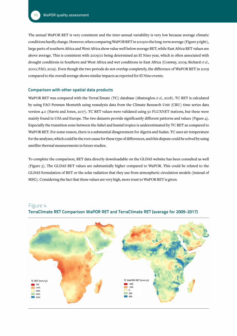
Comparison with other spatial data products
WaPOR RET was compared with the TerraClimate (TC) database (Abatzoglou et al., 2018). TC RET is calculated
by using FAO Penman Monteith using reanalysis data from the Climate Research Unit (CRU) time series data
version 4.0 (Harris and Jones, 2017). TC RET values were validated using 50 FLUXNET stations, but these were
mainly found in USA and Europe. The two datasets provide significantly different patterns and values (Figure 4).
Especially the transition zone between the Sahel and humid tropics is underestimated by TC RET as compared to
WaPOR RET. For some reason, there is a substantial disagreement for Algeria and Sudan. TC uses air temperature
for the analyses, which could be the root cause for these type of differences, and this dispute could be solved by using
satellite thermal measurements in future studies.
To complete the comparison, RET data directly downloadable on the GLDAS website has been consulted as well
(Figure 5). The GLDAS RET values are substantially higher compared to WaPOR. This could be related to the
GLDAS formulation of RET or the solar radiation that they use from atmospheric circulation models (instead of
MSG). Considering the fact that these values are very high, more trust to WaPOR RET is given.
Figure 4 TerraClimate RET Comparison WaPOR RET and TerraClimate RET (average for 2009-2017)
tc ret (mm/yr) tc wapor ret (mm/yr)7501375200026253250
-500-2500250500

112. Climate
Figure 5 GLDAS RET and comparison with WaPOR RET for the year 2010
Point data comparison
Full-fledged weather stations generally measure all parameters required to calculate RET using the Penman-
Monteith equation. Therefore, station RET was compared to WaPOR RET for a number of locations. Since the
WaPOR RET data has a spatial resolution of 20 km following MERRA no perfect correlation with station data can be
expected. The first comparison uses data from a weather station at Port Said, Egypt. Results are displayed in Figure
6. The linear regression indicates that the station data and WaPOR data have a good correlation with an R2 of 0.94. In
comparison with the 1:1 line the WaPOR RET data is consistently lower by 17 percent compared to the station data.
A second location is the Tal Amara weather station in the Bekaa Valley in Lebanon. For this station, surrounded
by agricultural fields, a longer time series of data was available, but for some periods data was not recorded (e.g.
radiation in early 2016) resulting in gaps (Figure 7). The WaPOR RET data follow the seasonality of the station data.
The r2 between the two datasets (2014-2016) is lower than for the Port Said station at 0.89, but is still relatively good.
Tests with more weather stations should be done to improve the accuracy of the quality assessment.
B.3 ConclusionsOn the continental level, variations in RET are low (varying less than 25 mm per year, 0.6%), due to similarity in
climatology between consecutive years. The WaPOR RET data is able to identify the impacts of the 2009 El Nino
event, with higher than average RET in Southern and Western Africa and lower RET values in East Africa. The
station comparison (only two stations) gives high correlation with the WaPOR data. This suggests that MERRA
is a good choice for computing RET, being an attractive solution for areas not being equipped with routine and
complete weather stations.
gldAs ret (mm/yr) gldAs - wapor ret (mm/yr)
7501375200026253250
-200-1500-100-5000

12 WaPOR quality assessment
Figure 6 RET from Egypt Port Said Station and WaPOR RET for 2014 – 2015
Figure 7 RET station data and WaPOR RET data for Tal Amara, Lebanon
! (X !,! - . / 0 !
0
1
2
3
4
5
6
7
8
9
10
11
0 1 2 3 4 5 6 7 8 9 10 11
WaP
OR v
1 RE
T [m
m/d
ay]
Station RET [mm/day]
!!1:1 line
Linear regression
! (a !,! - . / 0 !
0
2
4
6
8
10
12
RET
[mm
/day
]
01/01/2012
01/03/2012
01/05/2012
01/07/2012
01/09/2012
01/11/2012
01/01/2013
01/03/2013
01/05/2013
01/07/2013
01/09/2013
01/11/2013
01/01/2014
01/03/2014
01/05/2014
01/07/2014
01/09/2014
01/11/2014
01/01/2015
01/03/2015
01/05/2015
01/07/2015
01/09/2015
01/11/2015
01/01/2016
01/03/2016
01/05/2016
01/07/2016
01/09/2016
Station RET WaPOR RET

133. Water
3. Water
A. Actual evapotranspiration and Interception A.1 IntroductionThe Actual Evapotranspiration and Interception (AETI) flux is dependent on the availability of energy, the prevailing
Leaf Area Index (LAI) and soil moisture. AETI is an important component in the water balance, accounting for up
to 90 percent of the consumption of incoming precipitation in river basins such as the Nile system. It is of major
importance for disciplines ranging from hydrology to agricultural and climate sciences (Łabędzki, 2011; Trambauer
et al., 2014). Scientists have struggled to measure AETI in the field and have resorted to calculating it indirectly
through crop coefficients assuming conditions and crop development stages that follow certain specific standards
not considering diseases nor nutrient status (Allen et al., 1998). Direct measurements of AETI by for instance flux
towers, surface renewal or scintillometers are scarce in Africa and only available for a few point locations (flux
towers) or for small spatial extents (<5 km) for limited periods of time (scintilometer) as part of academic research
(Trambauer et al., 2014; Kongo et al., 2011). For the AETI at field and river basin scale, it is customary to use remote
sensing techniques to assess AETI because hydrological and crop growth models cannot capture the complex
ecosystem and biophysical dynamics induced by humans (land use and soil moisture) and nature (diseases; fungi;
salinity).
Det
ail o
f WaP
OR
Map
“A
ctua
l Eva
poT
rans
pira
tion
and
Inte
rcep
tion
(E
TIa
) - 1
- 10
May
201
9 - C
entr
al a
nd s
ub S
ahar
an A
fric
a”

14 WaPOR quality assessment
AETI is not directly measured by satellites. Instead, AETI can be determined from other terms of the surface energy
balance, calculated through physical variables that can be observed from space. Therefore various types of remote
sensing algorithms for the estimation of AETI have been developed. IHE Delft is making ensemble predictions of
AETI using seven different standard models. In addition, there exist AETI data layers based on flux measurements,
climate models and machine learning algorithms. A recent overview is provided by Pôcas et al. (2015) and Paca et al.
(2019).
Various studies evaluate AETI at large scales using inter-comparison of AETI estimations derived from different
types of models (Fisher et al., 2017; Jiménez et al., 2011; Kiptala et al., 2013; Miralles et al., 2016; Mu et al., 2011; Schuol
et al., 2008; Trambauer et al., 2014; Vinukollu et al., 2011; Wartenburger et al., 2018; Zhang et al., 2016). The differences
found between the models arise from inconsistencies in the use of forcing data, model conceptualization and user
defined parameter estimations and in the calculation method for AETI. Thus, when comparing magnitudes and
spread of AETI between the different approaches it is difficult to assess which model is more accurate than others,
specifically since there is limited ground observations to validate the data.
The WaPOR AETI data estimates Transpiration (T), Evaporation (E) and Interception (I) individually and sums
them up as AETI = T + E + I. WaPOR is based on the ETLook model (Bastiaanssen et al., 2012; Samain et al., 2012 ).
ETLook is designed for automated processing, and is versatile as it allows for soil moisture as an input data layer.
I is calculated independently using parameters for vegetation cover, leaf area index and precipitation. Most other
multi-layer surface energy balance models require more input data that are either not available, or the model
schematization is too simple so that the outputs are no longer reliable. The FRAME consortium has developed
ETLook into an operational model.
A.2 Data analysisWaPOR AETI shows similarities to the PCP dataset (Figure 8), the availability of water is clearly the constraining
factor for AETI. Energy (RET) plays a key role in equatorial Africa with frequent cloud cover and moist atmosphere.
Other areas with high AETI values are locations where water is available from surface runoff, flooding or groundwa-
ter presence for example the Inner Niger Delta in Mali, the Sudd wetland in Sudan, the Nile Delta and River in Egypt
and the Okavango Delta in Botswana (Figure 8). At continental scale, average annual AETI shows little variation
from 496-519 mm per year (Table 6).
Table 6 WaPOR AETI 2009-2017
2009 2010 2011 2012 2013 2014 2015 2016 2017 Average
Min 0 0 0 0 0 0 0 0 0 0
Max 2 336 2 243 2 213 2 217 2 154 2 183 2 191 2 216 2 285 2 226
Mean 505 497 496 497 488 500 499 513 519 502
Sd 516 490 508 492 497 505 504 513 521 505

153. Water
Figure 8 Average annual WaPOR AETI (2009-2017)
Comparison with other spatial data products
There are numerous spatially distributed AETI products available for Africa (Table 7). The products use different
input data and different approaches and vary in quality and spatial resolution. The WAter Cycle Observation Multi-
mission Strategy - EvapoTranspiration - WACMOS-ET (Michel et al., 2016), LandFlux-EVAL (Mueller et al., 2013),
and Model Tree Ensemble (MTE) (Jung, 2009) should also be mentioned in this regard. The LandFlux-EVAL covers
the period of 1989 to 2005, with a spatial resolution of 1o × 1o (Mueller et al., 2013)1. The MTE product is upscaled
from the database of the FLUXNET. The MTE ran for a longer period, from 1982 until 2011, spatially distributed on
a 0.5o × 0.5o grid (Jung et al., 2010)2. The WACMOS-ET Project has a better spatial resolution of 0.25o × 0.25o, for the
period 2005 to 2007 (Michel et al., 2016). The WACMOS-ET product is a combination of LandFlux-EVAL and MTE,
1 https://data.iac.ethz.ch/landflux/2 https://www.bgc-jena.mpg.de/geodb/projects/Home.php

16 WaPOR quality assessment
and thus expected to be superior. The development of each product has been peer reviewed, however with limited
observed AETI data to validate the accuracy over Africa and the Middle East.
Table 7 Statistics of AETI products over Africa 2010
Satellite product AETI estimation approach Source of input data
Reference
ETMonitor Process based model implementing processes of energy balance, plant physiology, and Soil water balance
MODIS, Microwave data
Hu and Jia, 2015
CMRSET based on priestley-taylor equation and relation between evI and gvmI
MODIS Guerschman et al., 2009
SEBS Calculates the energy balance, by calculating the sensible heat flux based on local maxima and minima of surface temperature
MODIS Su, Z. 2002
GLEAM v3.2 Based on Priestley-Taylor Equation (ETpot) multiplied by soil stress factors based on soil properties and interception is added based on CMORPH and TRMM
AMSR-E, LPRM, CMORPH, TRMM
Miralles et al., 2011a and b
SSEBop v4 Combines ET fractions generated from RS LST with reference ET using a thermal index approach.
MODIS Senay et al. 2014
ALEXI Calculates the evaporative fraction based on the morning and evening overpass of MODIS. Based on this fraction the ETa is determined.
MODIS, GOES Anderson et al., 2007
MODIS16 Combines the Penman Monteith equation and the surface conductance model.
MODIS Mu et al., 2007; 2011b
LandFlux-EVAL The LandFlux-EVAL covers the period of 1989 to 2005, with a spatial resolution of 1o × 1o (https://data.iac.ethz.ch/landflux/)
- Mueller et al., 2013
WACMOS-ET The WACMOS-ET product is a combination of LandFlux-EVAL and MTE, and thus expected to be superior
Various Michel et al., 2016
Model Tree Ensemble
The MTE product is upscaled from the database of the FLUXNET
Various Jung et al., 2009
GLDAS NOAH land surface models with remote sensing data assimilation
MODIS and ASCAT
Rodell et al., 2004
TerraClimate Water Balance Model outlined by Dobrowski et al. 2013
WorldClim version 2
Abatzoglou et al., 2018
WECANN Artificial Neural Network MODIS Alemohammad et al., 2017

173. Water
Table 8 shows the general statistical values of 11 remote sensing AETI products and Figure 9 shows the annual AETI
for WaPOR and ten similar databases for the year 2010. All products have similar spatial variabilities, identifying the
arid regions (Sahel and Middle East) and the majority can pick up high AETI values in the Nile Delta and the irrigated
agriculture along the Nile River. The average AETI of ten non-WaPOR product is 442 mm/yr with a minimum of 323
mm/yr (GLEAM) and a maximum of 570 mm/yr (CMRSET). The WaPOR estimate is 497 mm/yr, and this is a rather
average value, being 12 percent different from the average value.
Table 8 Statistics of AETI products over Africa 2010
WaPOR ETMonitor CMRSET SEBS GLEAM SSEBop ALEXI MODIS16 MTE GLDAS WECANN
Min 0 0 0 0 0 0 0 0 0 0 0
Max 2 243 2 414 2 567 1 730 1 953 2 808 2 010 1 828 1 407 1 689 1 177
Mean 497 402 570 376 323 497 519 402 418 468 434
Sd 490 423 466 396 1425 498 492 279 407 415 359
Figure 9 Comparison of the spatial distribution of AETI for 2010 from different products
wapor
gleAm v3.2
mte
et monitor
ssebop v4
gldAs
cmrset
AleXI
wecAnn
sebs
mod16
015037575011001500
bAckground
AetI (mm/yr)

18 WaPOR quality assessment
Comparing the AETI products, the following observations can be made. The spatial resolution of GLEAM,
WECANN, MTE and GLDAS is too low to pick up detailed spatial variations, such as the irrigated areas around the
Nile River. The MODIS16 product compared to the other products generally underestimates AETI, and does not
provide data for the arid regions. From the other six products, the main differences occur in the central part of the
African continent. ETmonitor and SEBS underestimate AETI in central Africa compared to the other four products.
This area has a high percentage of cloud cover, which affects also the WaPOR AETI data. ETmonitor combines
optical and microwave sensors and as such being capable of calculating AETI during cloudy periods. Similarly,
CMRSET and ALEXI seem to overestimate AETI in the arid areas, with some unrealistic values observed in Libya
and Chad. The spatial distribution of AETI in WaPOR and SSEBop are remarkably similar. This can be attributed
to the fact that both algorithms are based on the surface energy balance principles and make use of an internal
calibration of hot and cold edges.
It can be concluded that the WaPOR AETI data does not contain obvious flaws such as it is witnessed for some of
the other AETI databases. At continental level WaPOR AETI provides data that is at par with the other high quality
products. It also provides it at very high spatial and temporal resolution.
Comparison of AETI product based on water balance model (TerraClimate)
The WaPOR AETI was compared with the TerraClimate AETI product (Figure 10). This product is derived using
the water balance approach (Abatzoglou et al., 2018). The overall trend between the two products is very similar;
the major differences are found in irrigated areas, such as the Nile Delta, and in the Sudd Wetland in Sudan.
TerraClimate AETI is not able to pick up the increase in AETI due to irrigation and flooding in those areas, which
WaPOR does.
Figure 10 TerraClimate AETI product compared to WaPOR AETI
tc AetI (mm/yr) tc - wapor AetI (mm/yr)037575011251500
-1000-50005001000

193. Water
Comparison using continental scale water balance The WaPOR AETI was evaluated at river basin level using the classical water balance approach (WB). The long term
WB assumes a negligible change in storage, and therefore the total inflow (PCP) should be equal to the total outflow
(AETI and discharge (Q)) and therefore AETI should be equal to PCP minus Q (equation 1):
AETI=PCP-Q eq 1
The information on Q and PCP was obtained from external datasets. WB AETI was compared to WaPOR AETI. For
the comparison in Figure 11, the observed Q was obtained from the Global Runoff Data Centre (GRDC)3 (see Annex
A for locations of the data points) and for PCP we used the EWEMBI reanalysis PCP data (Dee et al., 2011). Figure 11
shows the value of AETI inferred from the WB for three key river basins in Africa (Congo, Niger and Nile basin), as
well as for two sub-basins in the Nile basin (inset of Figure 11). The Nile basin covers an area of 3.17 M km2, which
represents some 10 percent of the African continent. With 6 825 km, the Nile is the longest river in the world. It
has two main tributaries: (i) the White Nile originating from the Equatorial plateau of East Africa and (ii) the Blue
Nile, with its sources in the Ethiopian highlands. WB AETI for Congo, Niger and Nile are 1 206, 607 and 667 mm/yr
respectively. The corresponding WaPOR AETI estimates are 1 266 mm/yr (5.0% difference), 591 mm/yr (2.6% differ-
ence) and 668 mm/yr (0.0% difference) which is very encouraging.
s in charge of water management (Needs Assessment Report, 2016).
3 The Global Runoff Data Centre, 56068 Koblenz, Germany
Figure 11 GRDC stations in Africa and the spatially averaged AETI determined from the water balance of the Congo, Niger and Nile basins
Source: GRDC
et (mm)gauging stations river network upper blue nile blue nilenile

20 WaPOR quality assessment
A similar WB approach has been executed for an additional 28 basins in Africa (Figure 12). The average absolute
difference between the two datasets is 14 percent (ranging between 0 and 58%); combining all river basins the
difference is 0.2 percent (the over- and underestimation for individual basins is evened out at the continental
level). The largest difference occurs in smaller river basins. It can be noticed that WaPOR AETI is systematically
under-estimated in the in semi-arid climate zones such as Groot, Olifants and Orange. These South African basins
are all containing sparse vegetation areas, likely the cause factor for low basin-wide AETI values. Considering that
the method did not consider longer-term water storage changes in the water balance analysis, the difference of 14
percent is remarkably good.
Five other AETI data layers have been consulted for a comparative analysis in the same 28 river basins (with varying
periods of available data) (Table 9). While WaPOR AETI was 846 mm/yr, PCP-Q for the same basins was 847 mm/
yr. This is a very good agreement and shows congruency of WaPOR AETI with basin scale water balances. Next to
WaPOR, SSEBop provided a good match with 811 mm/yr. WaPOR and WECANN (Alemohammad et al., 2017) have
the highest correlation, but on overall, WaPOR AETI performs best.
Figure 12 Comparison of WaPOR and WB AETI for 28 selected river basins covering the period 2009 to 2017
0200400600800
10001200140016001800
AETI
[mm
/yr]
Awash
Bandama
Blue Nile Buzi
Cavally
Congo
Cunene
GambiaRufiji
Sassandra
Save
SenegalTa
na
Upper Blue Nile Void
ZambeziGroot
Komoe
WB
Lake Chad
Limpopo
MaputoMono
NigerNile
Okava
ngoOlifa
nt
Orange
Queme
WaPOR
Table 9 Comparison of various AETI products for the 28 river basins specified in Figure 12 (See Annex B for details per basin)
PCP-Q (observed)*
WaPOR (2009-2017)
GLEAM (1980-2013)
MOD16(2000-2014)
SSEBop(2003-2017)
WECANN(2007-2015)
MTE(1983-2012)
Average [mm/yr] 847.21 845.64 550.39 676.75 810.54 697.71 694.18
Average [mm/yr] 787.45 822.3 550.10 575.90 760.99 636.77 661.23
Correlation 0.92 0.89 0.90 0.89 0.92 0.89
Difference [mm/yr] 34.83 237.34 211.55 26.45 150.67 126.22
* different time periods

213. Water
Comparison with SWAT+ for Africa
A hydrological SWAT+ model was set up for Africa to compare the WaPOR AETI layers with AETI outputs from
the SWAT+ model. SWAT+ has been widely used to support water resources and agricultural management at river
basin scale (Arnold et al., 1998). A detailed description of the model setup is provided in Annex A. The comparison
of WaPOR and SWAT+ AETI shows areas where SWAT+ AETI is significantly lower than WaPOR AETI (green areas
in Figure 13). These areas correspond with irrigation areas and wetlands (e.g. Lake Chad and Inner Niger Delta in
arid zones), which are not implemented in SWAT+ and which are known to have high evapotranspiration. Global
irrigation maps also indicate these areas as irrigation areas. For that reason, we conclude that the values of WaPOR
are more realistic than SWAT outputs.
Figure 13 Long-term annual average AETI estimates by (left) WaPOR (2009-2017) and (right) SWAT+ (2010-2016) and difference between WaPOR and SWAT+ AETI for Africa (below)
(mm/yr)
0
500
1000
1500
2000
(mm/yr)
-1500-500010002500

22 WaPOR quality assessment
In some areas, we see that the SWAT+ AETI is significantly higher compared to WaPOR AETI (in red in Figure 13).
These areas are predominantly located in forested areas (Annex A) where high evaporation can be expected. One
of these areas is located in the Congo basin. We compared WaPOR and SWAT+ AETI with a mass balance analysis
(PCP-Q) for the three major basins in Africa and a selected number of sub-basins (Table 10). The results suggest
that the WaPOR AETI results are more realistic. It is however advised to further explore and evaluate the WaPOR
AETI results of forested areas.
As a general conclusion, the comparison of SWAT+ and WaPOR leads to a confirmation of the WaPOR results. In
most areas, the difference between the two methods is small and within the range of uncertainties of both methods.
At locations with large differences, the WaPOR results seem to be more realistic. This confirms the advantage of
using indirect earth observations of the AETI process.
Basin comparison – Litani River Basin
The Litani River Basin is located in Lebanon and covers an area of 2 170 km2. The basin is the focus of a Water
Accounting study using WaPOR data inputs (Tran et al., 2019). This section validates the overall water balance using
WaPOR data. Table 11 has been compiled to evaluate WaPOR PCP and AETI data for the entire basin. The average
WaPOR PCP-AETI value is 624 - 436 being 188 mm/yr, or 408 Mm3/yr.
The Litani River Authority (LRA) provided outflow data at the Qasmiye (Sea Mouth) gauging station to support the
analysis of this project. During the wet year 2012, the total outflow was 360 Mm3/yr, but the flow into the sea reduced
to 60 Mm3/yr during 2014, a dry year. The 5-year average outflow between 2011 and 2015 is 193 Mm3/yr. For an area of
2 170 km2, this represents a water yield of 89 mm/yr. This is equivalent to 14 percent of the gross rainfall.
Table 10 Comparison of AETI estimates using PCP-Q, WAPOR and SWAT+ for basins in Africa
PCP-Q WAPOR SWAT+
Basin Name AETI [mm/yr] Period AETI [mm/yr] Period AETI [mm/yr] Period
nile 667 1912-1984 668 2009-2017 578 2010-2016
blue nile 937 1960-1982 822 911
upper blue nile 1 135 1980-1982
1999-2002
955 1 114
niger 607 1970-2006 591 630
congo 1 206 1903-2010 1 266 1 276
lake victoria 1 091 1950-2005 1 035 976
lake victoria (lake surface)
1 539* 1993-2014 1 138 893
* based on study by vanderkelen et al., 2018

233. Water
Table 11 Comparison of annual P and ET values for the entire Litani Basin based on the original WaPOR data.
Year PCP(mm/yr)
PCP(Mm3/yr)
AETI(mm/yr)
AETI(Mm3/yr)
PCP - AETI(mm/yr)
PCP – AETI(Mm3/yr)
2009 746 1 619 484 1 050 262 569
2010 638 1 384 496 1 076 142 308
2011 633 1 374 439 953 194 421
2012 816 1 772 441 957 375 815
2013 741 1 608 491 1 066 250 542
2014 456 990 361 784 95 206
2015 530 1 150 424 921 106 229
2016 594 1 290 399 865 196 425
2017 461 1 000 387 839 74 161
Average 624 1 354 436 946 188 408
Next to the river discharge into the ocean, the Litani Basin also has a significant interbasin transfers. The main
interbasin transfer is the water drawn from Qaraoun Lake after hydropower production at the Abd el Al station.
Through Markaba and Awali tunnels water is delivered to the urban settlements of Beirut and irrigated land outside
the watershed of the Litani. The discharge capacity of the tunnels is 22 m3/s4. However, the actual discharge in this
tunnel varies greatly between years (Figure 14), with an average discharge of 200 Mm3/yr from 2012-2016. Litani
water is also transferred into the Hasbani River, that lies in southern Lebanon and flows to Israel. There is also
water conveyed to Marjayoun, which is in the middle of the basin boundaries. The Qasimiya and Ras Al Ain irrigation
project, which is one of the most important irrigation projects in Lebanon, draws water from the river before the
basin outlet at sea mouth with discharge capacity of approximately 5 m3/s. The water is conveyed to villages in Sidon
and Maachouk, both are outside of the basin5. Since monthly discharge by these several inter-basin water allocation
projects are not reported, it is infeasible to quantify the total inter-basin transfer on a monthly basis.
The uncertainty in inter-basin transfer makes it difficult to estimate actual water availability. In the Litani Basin,
the long-term water storage trend should be considered in the analyses. This information was obtained from the
GRACE satellite, which shows a negative trend in storage (∆S) (Figure 15). The trend of water storage for a single
GRACE pixel that covers central Lebanon from 2009 to 2016 is -21mm/yr, which is translated into -43.5 Mm3/yr in
the Litani Basin.
4 The Litani River Authority - Power Stations and Tunnels (http://www.litani.gov.lb/en/?page_id=95)5 The Litani River Authority - Qasimiya and Ras Al Ain Irrigation Project (http://www.litani.gov.lb/en/?page_id=117)

24 WaPOR quality assessment
Figure 14 Discharge in Markaba tunnel after hydropower turbines at Abd el Al station
Figure 15 Longer-term trend of declining water storage in Lebanon based on GRACE gravity measurements
The uncertainty in inter-basin transfer makes it difficult to estimate actual water availability. Nevertheless,
total discharge measured at the sea mouth outlet and Markaba tunnel is approximately equal to PCP – AETI - ∆S
for the year 2012 and 2013 (Figure 16; Table 12), which means that the total WaPOR AETI for the basin covering
heterogeneous land use is reasonable.
Source: https://ccar.colorado.edu/grace/gsfc.html
0
2
4
6
8
10
12
14
16
18
20
Disc
harg
e [m
3 /s]
12.03.2011 12.03.2012 12.03.2013 12.03.2014 12.03.2015 12.03.2016
2009 2011
mascon#:9492
lat: 33.66
lon: 36.02
trend: -0.21 cm/yrAnnual Amplitude: 2.47 cmsemi-Annual Amp.: 0.74 cmgsfc mascons ,mascon #9492
2006
2013
2010
2015
2014
2010
2004
2012
2008
2014
2012
2016
2016
8
6
4
2
0
-2
-4
-6
-8
-10

253. Water
Figure 16 Total discharge from Litani outlet at sea mouth and Markaba tunnel compared with PCP – AETI – ΔS, based on remote sensing data
Sub-basin comparison – Nile BasinThe AETI in the Nile basin has been estimated by various authors using various methods (NBI, 2014; Belete et al.,
2018; Bastiaanssen et al., 2014; Hilhorst et al., 2011; Senay et al., 2009; Jung et al., 2017). The WaPOR AETI values (entire
basin, Blue Nile and Upper Blue Nile) were compared to the estimates of the other studies and compared to the
Water Balance using observed data (Table 13).
0
2
4
6
8
10
12
14
16
Mm
3 /yea
r
2010
Q_seamouth Q_Markaba P-ET-ds
2011 2012 2013 2014 2015 2016
Table 12 Average annual water balance components of the Litani River Basin using WaPOR data inputs
Year Qseamouth QMarkaba PCP ΔS PCP-ΔS-Q WaPOR AETI
2010 183.0 200 1,319 -65 1,001 1,026
2011 194.3 200 1,310 -72 988 908
2012 357.2 400 1,689 35 897 912
2013 196.1 381 1,533 -77 1,033 1,016
2014 62.6 73 943 -25 832 747
2015 167.9 116 1,096 -99 911 878
2016 91.2 120 1,229 -38 1,056 825
Average 178.9 213 1,303 -49 960 902

26 WaPOR quality assessment
Even-though the AETI estimates refer to different time periods, the WaPOR AETI values (688 mm/yr) are similar
to the WB AETI values (667 mm/yr). Bastiaanssen et al. (2014) used a calibrated version of the SSEBop model and
concluded that the total AETI was 633 mm/yr for the period 2005 to 2010. Karimi et al. (2012) for a single year (2017)
estimated the basin-wide AETI to be 622 mm/yr. Senay et al. (2014) estimated the average AETI to be 702 mm/yr and
the volume 2 056*109 m3/yr. The WaPOR AETI estimates of 668 mm/yr are within the expected range (545 to 700
mm/yr; average 638 mm/yr). Considering that WaPOR AETI is within 5 percent of the other estimates, it is believed
that the AETI volume for the Nile Basin by WaPOR is highly accurate. This is in agreement with the other finding of
the Congo, Niger, Litani and the 28 basins presented in Figure 12.
A more detailed breakdown comparison of the Nile System could be achieved from comparison against the FAO
Nile study (Hilhorst et al., 2011). The program for the hydrology and water resources management of the Nile Basin
ran between 2004 and 2009. The main project objective was to contribute to the establishment of a common knowl-
edge base at the Nile Basin level. The AETI under FAO Nile was computed by a combined approach of water balance
(rainfall, discharge) and crop water requirements. There are thus no direct measurements of AETI, yet this will be
considered as “ground truth”. For the climatic inputs of this study, the average observation period between 1960 to
1990 has been used in FAO Nile.
Table 13 Comparison of AETI estimates using the water balance, WaPOR and past studies in the Nile Basin
Basin Name
WaPOR Water Balance (WB) Other Studies
AETI [mm/yr]
Period AETI [mm/yr]
Period Model AETI [mm/yr]
Period reference
Nile
668
2009-2017
667 1912-1984
Improved MOD16 algorithm
545 2000-2012
Nile Basin Initiative, 2014
InVEST 700 1950-2000 Belete et al. 2018
Nile-DST 628 1960-1990 Hilhorst et al. 2011
Adjusted SSEBop 633 2005-
2010Bastiaanssen et al. 2014
ETLook 622 2017 Karimi et al., 2014
SSEBop 702 2000-2012 Senay et al. 2014
Blue Nile
822 937 1960-1982
Adjusted SSEBop 737 2005-
2010Bastiaanssen et al. 2014
Nile-DST 863 1960-1990 Hilhorst et al. 2011
Upper Blue Nile
955 1 1351980-1982
1999-2002
VegET 500 2001-2007 Senay et al., 2009
Noah3.3-M2
CLSMF2-M2
ALEXI
GLEAM
909
1 010
979
675
2007-2010 Jung et al. 2017

273. Water
Table 21 of the FAO Nile synthesis report describes the (i) AETI over land, (ii) AETI over open water and the (iii)
AETI over wetlands. The total AETI is also provided and used for the validation of WaPOR. The FAO-Nile team has
defined 11 sub-basins of the Nile. Since we did not have access to digital boundaries, the shape file provided by the
Nile Basin Initiative has been used instead. The sub-basins between FAO Nile and NBI are not matching exactly as
Figure 17 Geographical location of the sub-basins according to NBI
can be observed from the area statistics presented in
Table 14. FAO Nile covers a total area of 3.17 million
km2 while NBI adds up to 3.24 million km2. For these
reasons, the AETI data was compared per unit of
land instead of considering a bulk volume.
The total annual AETI for the Nile according to
FAO Nile – here considered as ground truth – is 1
991*109 m3/yr (i.e. 628 mm/yr). WaPOR AETI shows
2 052*109 m3 for a 2.2 percent larger area. The differ-
ence in volumetric AETI of 61 109m3/yr is 3 percent,
hence after correction for area the two values are
remarkably similar.
The correlation coefficient for all the sub-basins is
with R2 of 0.93 very encouraging. The lower AETI
rates of the lower Nile in Northern Sudan and
Egypt is very accurate. More deviations arise in the
tropical sub-basins of the Baro – Akobo – Sobat
and Lake Victoria, which is most likely related to
cloud cover as a disturbing factor on the determina-
tion of the land surface evapotranspiration. Over-
estimations and under-estimations are in perfect
balance (Figure 18), which can also be related to the
inaccuracy of the “ground truth” and ascribed to
different study periods. This shows that the total
WaPOR AETI for large sub-basins of typically 300
000 km2 with rather diverging climates and land use
is accurate.Source: Nile Basin Initiative - http://www.nilebasin.org/
bahr el ghazal
bahr el Jebel
baro Akobbo sobat
blue nile
lake Albert
lake victoria
main nile
tekeze Atbara
victoria nile
white nile

28 WaPOR quality assessment
Table 14 AETI statistics per sub-basin according to FAO-Nile and WaPOR
FAO Nile WaPOR
Area AETI Area AETI
(km2) (mm/yr) (109m3/yr) (km2) (mm/yr) (109m3/yr)
main nile d/s Atbara 877 866 124 109 986 111 120 119
Atbara 237 044 397 94 232 321 416 97
main nile d/s khartoum
34 523 211 7 35 458 179 6
blue nile 308 198 863 266 308 474 792 244
white nile 260 943 554 145 238 349 575 137
bahr el ghazal & el Arab
606 428 749 454 720 012 885 637
pibor-Akabo-sobat 246 779 907 224 231 352 1 147 265
bahr el Jebel 136 400 1 196 163 80 789 1 196 97
kyoga-Albert 197 253 1 124 222 157 541 1 250 197
lake victoria basin 264 985 1 160 307 250 549 1 013 254
total 3 170 419 628 1 991 3 240 957 633 2 052
*slight difference in area is a result of the delineation of the sub-basins
Figure 18 Relationship between the longer-term total FAO-Nile and WaPOR AETI per sub-basin of the Nile

293. Water
Table 15 Annual AETI (mm/yr) of the land use class irrigated land in Fayoum Depression
2009 2010 2011 2012 2013 2014 2015 2016 2017 Average
WaPOR 802 877 759 846 850 941 965 941 961 882
ALEXI 726 735 748 742 751 742 759 743
CMRSET 604 663 640 636 636
ETMonitor 423 430 458 435 466 441
MODIS 312 285 334 306 331 333 317
SSEBop 822 802 876 844 883 837 888 855 861 852
SEBS 194 216 149 198 187 159 191 147 180
ETensemble* 1 110 1 099 1 155 1 122 1 122
* ensemble created using etmonitor and ssebop by salvadore (2019)
Sub-basin comparison - Fayoum DepressionThe Fayoum Depression in Egypt has a well established water balance due to its depression character and irrigation
supply through one single main canal, and was therefore explored for validation purposes. Following Salvadore et
al. (2019) - who summarized the water balance from various sources- the water balance for the gross area including
Lake Qarun reads as:
AETI = PCP + Q - q
With
PCP = 20 Mm3/yr
Irrigation supply Q = 2 900 Mm3/yr
Return flow q = 250 Mm3/yr
Over a year, the change in storage was assumed zero and the recharge to groundwater assumed negligible (Salvadore,
2019). The resulting AETI from the total oasis then becomes 2 670 Mm3/yr, equivalent to 882 mm/yr (Table 15). This
is much lower than the potential AETI of 1 420 mm/yr as suggested by Ramadan et al. (1989). The irrigation supply of
2 900 Mm3/yr per unit of land is 1 827 mm/yr being equivalent to a planned irrigation efficiency of 78 percent to meet
the crop water requirements (1,420/1,827 x 100%). It is likely that AETI is lower than 1 420 mm/yr because salinity
persists and crops in Fayoum are not expected to evaporate at their potential rate. Wolters et al. (1989) approximated
the AETI to be 1 100 mm/yr, and this seems more realistic than the 882 mm/yr found for WaPOR.
For the irrigated area of 158 734 ha displayed in Figure 19, the total AETI from WaPOR is 1 400 Mm3/yr. Ramadan
et al. (1989) estimated the total crop water consumption to be 1 460 Mm3/yr, being very close to WaPOR AETI. We
believe however, that different areas are considered, which could explain the fact that the volumetric AETI values
are similar, and the water depths are not. The irrigation efficiency becomes 48 percent (1.4/2.9 x 100%), which seems
low for a classical flood irrigation scheme with reuse of drainage water. Even though WaPOR AETI estimates are
about 20 percent lower than expected, other remote sensing products show even lower estimates for AETI (Table
15). Salvadore (2019) created an ETensemble product using ETMonitor and SSEBop with a bias correction factor to
be able to create an AETI product which resembles the actual situation.

30 WaPOR quality assessment
Figure 19 Location of the Fayoum Depression in Egypt. The polygons indicate irrigated areas
Field scale flux measurementsObserved AETI data in Africa is very limited,
as flux towers are very expensive. Eddy covari-
ance flux data is often considered the “gold”
standard for the estimation of AETI, however,
even these measurements can have up to 15-20
percent error. The eddy covariance data is
compared with WaPOR data using the pixel
available at the coordinates of the flux tower.
The assumption is that the point data meas-
ured by the flux tower captures the average
value of the grid cell (Marshall et al., 2013). This
assumption is more likely when the station lies
within homogeneous and flat terrain. If this is
not the case, eddy covariance may vary signifi-
cantly and may not be representative for the
grid cell value (Baldocchi et al., 1988).
We obtained data from seven stations. The FLUXNET database 6 provided data for three stations in Africa, in
Ghana, Senegal and South Africa. The three sites have distinctive differences in land use. The site in Ghana is located
in the Ankasa national park, which is located in a primary tropical forest (Chiti et al., 2010; Marchesini et al., 2011;
Valentini et al., 2016). The site in Senegal is located in Dahra, a village at the verge of the Sahel (Tagesson et al., 2015;
doi: 10.18140/FLX/1440188). The third site is located in the Kruger national park (Skukuza), with shrubs and other
low vegetation (Archibald et al., 2009; doi: 10.18140/FLX/1440246). In addition, we got access to flux data from three
stations in South Africa over irrigated crops from the Universities of KwaZulu Natal (grapes and sugarcane) and one
station in Egypt from the University of Tsukuba (various crops typically found in Egypt).
A 250 m (WaPOR Level 1) or 100 m (WaPOR Level 2 – only available for Ghana and Egypt) footprint is in fact too
large for properly representing the footprint of flux towers because most contribution on the measured atmos-
pheric water vapor originates nearer to the location of the flux tower (this within a single pixel). The pixel value is
in that case always a systematic underestimation, and this aspect needs to be considered in the analysis followed
hereafter. The data is provided at daily time steps, whilst the WaPOR AETI data is available at decadal (10 days) time
steps. For this reason, the eddy covariance data is first averaged per decadal and then compared with the WaPOR
AETI time series.
The WaPOR AETI decadal data is plotted against the FLUXNET data in Figure 20 (time series comparison are found
in Annex C). For each station there are periods where the station AETI values are not consistent with observed
trends, and these periods were removed from the analyses (Annex C). Only one of the stations show good correla-
tion between the station data and WaPOR data (Senegal WaPOR Level 1 – r2 equals 0.7), for the other stations r2
ranges between 0.1 and -1.1. The bias for the flux station in Senegal and South Africa are -3 percent and 4 percent,
respectively. For the station in Ghana, WaPOR AETI is systematically overestimated by 21 percent and 67 percent
for Level 1 and Level 2 respectively. Even though there is a large scatter between the flux tower and WaPOR AETI
data (Figure 20), the WaPOR AETI data is within the same ballpark as the flux tower data. There is an exception for
the flux tower in Ghana, compared with both the Level 1 and Level 2 data.
6 https://fluxnet.fluxdata.org/

313. Water
Three other eddy covariance datasets were made available by the University of Kwazulu Natal. The three flux towers
are located in agricultural areas: one in sugarcane and the other two in vineyards. Results of the comparison are
shown in Figure 21. The dataset of Komati (sugarcane) is for 2011 – 2012; for Vergelegen and Kapel (vineyard) it is
2013 – 2016. The dataset of Komati is a Surface Renewal system as described in Bastidas-Obando et al. (2017). The
dataset of Kapel and Vergelegen are based on one-sensor eddy covariance systems.
Figure 21 shows that for the sugar cane (Komati) dataset the WaPOR AETI layer compares reasonably well with the
flux tower results. Despite a good correlation, the WaPOR AETI estimates are higher than AETI values of the flux
tower by 23 percent. The comparison for vineyard data (Vergelegen and Kapel) indicates essential differences. The
values from WaPOR AETI are significantly lower than those found at the flux tower. Results show that the AETI
ranges from 0 to 2 mm/day, whereas the observations range from 0 to 5 mm/day with an overall bias of 60 percent.
In addition to cropland, the University of KwaZulu Natal installed a flux tower in the natural grasslands at Cathedral
Peak in South Africa. The station data shows good correlation with the WaPOR AETI data for pastures (Figure 22).
The largest outliers also have the highest number of missing days and potential error in the observations. During
this period, WaPOR AETI estimates are lower compared to the flux tower observations (Figure 22). Excluding
this period, the overall correlation between the WaPOR and observed AETI data is 0.66 with a bias of -33 percent,
The general trend of WaPOR AETI for pastures is very similar to the flux tower observations, however there is a
significant underestimation of the WaPOR AETI.
Figure 20 Comparison Fluxnet tower and WaPOR AETI
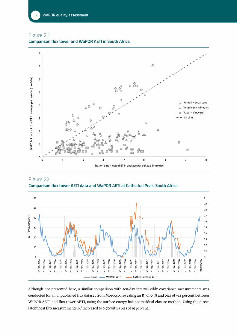
32 WaPOR quality assessment
Figure 21 Comparison flux tower and WaPOR AETI in South Africa
Figure 22 Comparison flux tower AETI data and WaPOR AETI at Cathedral Peak, South Africa
Although not presented here, a similar comparison with ten-day interval eddy covariance measurements was
conducted for an unpublished flux dataset from Morocco, revealing an R2 of 0.58 and bias of +12 percent between
WaPOR AETI and flux tower AETI, using the surface energy balance residual closure method. Using the direct
latent heat flux measurements, R2 increased to 0.70 with a bias of 19 percent.
komati - sugarcane
vergelegen -vineyard
kapel - vineyard
1:1 line
station data - Actual et in average per dekadal (mm/day)
8
7
6
5
4
3
2
1
00 1 2 3 4 5 6 7 8
wap
orv1
dat
a - A
ctua
l et
in a
vera
ge p
er d
ekad
al (m
m/d
ay)
01/0
1/20
14
01/0
3/20
14
01/0
5/20
14
01/0
7/20
14
01/0
9/20
14
01/1
1/20
14
01/0
1/20
15
01/0
3/20
15
01/0
5/20
15
01/0
7/20
15
01/0
9/20
15
01/1
1/20
15
01/0
1/20
16
01/0
3/20
16
01/0
5/20
16
01/0
7/20
16
01/0
9/20
16
01/1
1/20
16
01/0
1/20
17
01/0
3/20
17
01/0
5/20
17
01/0
7/20
17
01/0
9/20
17
01/1
1/20
17
01/0
1/20
18
01/0
3/20
18
01/0
5/20
18
01/0
7/20
18
01/0
9/20
18
01/1
1/20
18
01/
01/2
019
60
50
40
30
20
10
0
error wapor AetI cathedral peak AetI
AetI
(mm
/dec
ade)
1
0.9
0.8
0.7
0.6
0.5
0.4
0.3
0.2
0.1
0

333. Water
The comparisons between the observed flux tower data and WaPOR shows two different trends, a number of
stations show very good correlation or small bias despite the challenges between the pixel size and footprint of
the flux tower (e.g. Senegal, Skukuza, Komati and Cathedral Peak, South Africa). On the other hand, a number of
stations do not show good correlation or large biases. There are a number of possible reasons related to the spatial
uniformity of the land use. For example, sugarcane plantations have a more spatial uniform AETI behavior, which
eliminates the disturbing role of footprints in the validation exercise. However, the Level 2 data for Ghana did not
improve the correlation between the two datasets; in this case errors in the observed data could be an issue, and
Twine et al. (2000) indicated that AETI can be underestimated from 10 up to 30 percent. The comparative analyses
to point observations show that vineyards cannot be validated, but that sugarcane, grasslands and shrubs lay all
within the range of 0 to 30 percent uncertainty.
The University of Tsukuba (Japan) has installed various eddy covariance system in the Nile Delta of Egypt to
measure the complete energy balance under actual growing conditions of irrigated fields (Sugita et al., 2017).
While they have measured the energy balance under both traditionally irrigation methods and water savings using
different schedules and drip irrigation, this section of the report only deals with the flux measurements conducted
in the traditional irrigation treatments. The in situ fluxes were measured in the period 2010 to 2014, and we used
the values reported in Sugita et al. (2017) for comparison with the WaPOR AETI. Maize and rice are the summer
crops and fava beans and wheat the winter crops. Three different sites were installed with eddy covariance sensors,
and these sites are referred to as Sakha-A, Sakha-B and Zankalon. The Sakha-B site was used mainly for adjusted
irrigation schedules, so the analysis in this section mainly deals with Sakha-A. The annual AETI values measured
vary between 875 to 1 225 mm/yr, with an average value of 972 mm/yr (see Table 16). Matching WaPOR pixels have
been identified and a 3x3 window was selected for excluding the effect of geometrically inaccuracy. WaPOR suggest
the average value for Sakha-A in the period 2010 to 2014 to be 1 000 mm/yr. For Sakha-B the average value is 1 011
mm/yr and for Zankalon 1,295 mm/yr (Table 16). The ten-day data is presented in Figure 23. El-Quosy and El-Guindy
(1989) reported a typical AETI range of 1 056 to 1 275 mm/yr, depending on the climatic zone in the Nile Delta and
the associated cropping pattern in each of their four climate zones. The AETI of a single crop varies between 370 mm
(wheat) to 880 mm (cotton), so the actual cropping pattern determines the total AETI of a certain pixel or group of
pixels. This short synopsis reveals that the annual AETI totals of WaPOR are very close to the field measurements.
The ten day WaPOR AETI values are compared to the in situ flux measurements for crop development stages
(Sugita et al., 2017) and are presented in Figure 23. The peak flux measurements during summer are exceeding the
WaPOR AETI estimates; the WaPOR AETI values do not exceed 5.5 mm/d during ten-day periods, while the in situ
measurements suggest this can be as high as 6.5 mm/d for periods of ten days and longer (Sugita et al., 2017).
Table 16 Comparison of annual WaPOR and measured AETI on traditionally irrigated crops in the Nile Delta
Location Crop rotation Irrigation Measured AETI (mm/yr) WaPOR AETI (mm/yr)
sakha-A Maize & Fava beans Flood 875 1 000
sakha-b Rice & Wheat Basin 1 225 1 011
Zankalon Rice & Berseem Basin 816 1 295
Average 972 1 102

34 WaPOR quality assessment
A further breakdown of the annual AETI values is to evaluate the AETI fluxes per type of crop and per growing
season (see Table 17). Flooded maize in Sakha-A should typically evaporate 680-720 mm/season (Sugita et al., 2017),
whereas WaPOR AETI estimates 327-360 mm/season, typically 50 percent lower. The evaporation of the winter
crops (wheat and berseem) in Sakha-A is 511-608 mm/season, whereas WaPOR AETI values lay in the range of
391-487 mm/season, 9-26 percent lower. For Zankalon, the agreement for winter crops is much better with less
than 3 percent deviation (AETI measured is 446-549 mm/season and WaPOR AETI is approximately 448-561 mm/
season). The interim conclusion is that AETI of WaPOR during winter period is reasonable but that during the
summer it is significantly underestimated. Interestingly, at annual timescales, WaPOR AETI values are higher than
the observed AETI (1 102 mm/yr compared to 972 mm/yr), this difference originates from the fallow periods. This
is a point of attention, WaPOR AETI underestimates crop AETI (which is mainly T), and overestimates fallow land
AETI (which is mainly E).
Field soil water balance measurementsThe University of Oxford is conducting a special program in Jordan, Israel and Palestine on Water and Food Security
in the Middle East7. As part of this program, field measurements and farm interviews on different irrigated crops in
the Jordan Valley took place. Various field sites in Jordan and Israel were covered. Different vegetables are included
in the analysis, namely onions, bananas, berhis, citrus, madjoul, lemons, grapefruits and oranges. Additional
information can be found in Gilmont et al. (2018). Because of the wide variability in irrigation water supply gathered
from the field campaigns, we used average values for the nine different fields in Jordan and ten fields in Israel.
In the field sites in Jordan, the average PCP is 389 mm/yr and the irrigation supply (Irr) based on interviews and
measurements is 957 mm/yr (Table 18). The average WaPOR AETI is 728 mm/yr. The rest term of the soil water
balance represents the total runoff and drainage (assuming storage changes over the year is small). This yields in a
7 http://wanainstitute.org/en/publication/decoupling-national-water-needs-national-water-supplies-insights-and-potential-countries
Figure 23 Temporal variability of flux measurements and WaPOR AETI for the flux site Sakha-A
0
1
2
3
4
5
6
7
AETI
(mm
/d)
01.01.2010
WaPOR Flux measurement
01.01.2011 01.01.2012 12.31.2012 12.31.2013 12.31.2014

353. Water
large total runoff of 618 mm/yr. When assuming that 70 percent of PCP is available for AETI (runoff coefficient of
30%), the average AETI from irrigation (AETIirr) becomes 455 mm/yr, resulting in an on-farm irrigation efficiency
(Ieff) of 48 percent (455/957 x 100%). In reality, runoff is lower and efficiency higher. Because the calibration of the
Fayoum Depression indicated a bias correction of 1.2, the data was analyzed again with 1.2 x WaPOR AETI. The
result is a revised estimate of AETIirr_1.2 being 473 mm/yr and an associated Ieff_1.2 of 83 percent (Table 18). This seems
to be realistic values for micro-irrigation in Jordan. Hence, a bias correction of 1.2 on WaPOR AETI is required for
irrigated areas in Jordan.
For Israel, the amounts of applied water were acquired mainly from interviews and carefully verified in the field.
Lemons, grapefruit and oranges are included in the dataset. PCP is with 283 mm/yr lower than for Jordan, and
the irrigation supplies are higher 1 115 mm/yr. WaPOR AETI is with 549 mm/yr and derived irrigation efficiency of
32 percent unrealistically low and not in agreement with the significant water supplies of 1 115 mm/yr, and in the
presence of micro-irrigation (Table 19). Because a bias factor of 1.2 was insufficient, a correction factor 1.6 was
used. The runoff and drainage reduces then from 849 mm/yr to 520 mm/yr and the efficiency doubles from 32 to 63
percent. This is still a relatively low irrigation efficiency.
For both analyses (Jordan and Israel), the WaPOR AETI required a bias correction to obtain realistic results
for the field soil water balance analyses. This bias correction is meant for relatively small corrections, and
not as calibration coefficient. It must be noted that other components of the field soil water balance (PCP, Irr
and runoff ) are estimated and not measured. There is also a discrepancy between the small-scale agricultural
features of the Jordan Valley and the spectral resolution of 100 m and 250 m pixels, this may be fixed if the
Table 17 Seasonal measured and WaPOR AETI fluxes
Site Irr Crop Season AETI (mm/season)
Start End Duration Observed* WaPOR
sakha-A Flood Maize Summer 20-06-2010 01-10-2010 103 680 360
sakha-A Flood Maize Summer 14-06-2011 17-09-2011 95 632 335
sakha-A Flood Maize Summer 01-07-2013 10-10-2013 102 720 327
sakha-A Basin Wheat Winter 25-11-2011 08-05-2012 164 511 391
sakha-A Basin Wheat Winter 11-12-2012 13-05-2013 153 608 446
sakha-A Flood Sugarbeet Winter 07-11-2013 09-05-2014 182 538 487
Zankalon Basin Berseem Winter 26-10-2011 25-05-2012 211 549 561
Zankalon Flood Fava beans
Winter 08-11-2012 18-04-2013 177 446 448
* sugita et al., 2017

36 WaPOR quality assessment
Table 18 Components of the field scale soil water balance in irrigated vegetables in the Jordan Valley (in mm/yr); the Jordan component
Country Crop PCP Irr WaPOR AETI
Runoff AETIpcp AETIirr Ieff AETIirr_1.2 Ieff_1.2
Jordan Onion 400 567 937 30 280 657 116 844 149
Jordan Banana 400 856 909 347 280 629 74 811 95
Jordan Banana 400 1 433 683 1 150 280 403 28 540 38
Jordan Berhi 400 821 559 662 280 279 34 391 48
Jordan Citrus 350 881 780 451 245 535 61 691 78
Jordan Citrus 350 409 586 173 245 341 83 458 112
Jordan Berhi 400 2 022 686 1 736 280 406 20 543 27
Jordan Madjoul 400 374 734 40 280 454 121 601 161
Jordan Madjoul 400 1 248 674 974 280 394 32 529 42
Average 389 957 728 618 272 455 48 601 83
source: gilmont et al., 2019
Table 19 Components of the field scale soil water balance in irrigated vegetables in the Jordan Valley (in mm/yr); the Israel component
Country Crop PCP Irr WaPOR AETI Runoff AETIIrr Ieff AETIIrr_1.6 Ieff_1.6
Israel Onion 300 700 468 532 258 37 539 77
Israel Lemon 350 1 100 496 954 251 23 549 50
Israel Majool 215 1 600 650 1 165 500 31 890 56
Israel Barhi 215 1 400 740 875 590 42 1 034 74
Israel Banana 350 1 200 589 961 344 29 697 58
Israel Grapefruit 250 1 000 500 750 325 33 625 63
Israel Orange 250 1 000 505 745 330 33 633 63
Israel Madjoul 300 1 200 516 984 306 26 616 51
Israel Barhi 300 1 200 448 1 052 238 20 507 42
Israel Onion 300 750 578 472 368 49 715 95
Average 283 1 115 549 849 351 32 680 63
source: gilmont et al., 2019

373. Water
WaPOR Level 3 (30 m resolution) is available in the area. We also believe that the high aridity may play an additional
role in underestimating WaPOR AETI.
A.3 Conclusion Compared to similar remote sensing databases, the WaPOR AETI database is among the ones with the most realistic
signatures at larger scale and for time-integrated values. The comparison with the water balance of 28 river basins
is encouraging, and these findings were consistent with the basin analysis of the Congo, Niger and Nile system. The
results of the Litani Basin shows proper concurrency with the measured outflows to the Mediterranean Sea and
interbasin transfers. More uncertainty arises for smaller areas such as Fayoum Depression and Jordan Valley where
WAPOR AETI seems systematically underestimated by 20 percent and more. However, analyses of comparative
remote sensing products for the Fayoum area shows that WaPOR AETI preforms better than the other products,
with only SSEBop performing in similar fashion. Both Fayoum and Jordan Valley are located in semi-arid and arid
climates, and WaPOR AETI appears to underperform under arid conditions.
The advantage of flux towers is that shorter periods can be evaluated as well. The validation with individual flux
tower data suggests that peak fluxes during hot Egyptian summers are not met. Rarely WaPOR estimates fluxes
more than 5 mm/d during decadal time increments. The correlation with flux data for stations in South Africa varies
by location and land use. The more arid Western Cape has a lower performance than Cathedral Peak that is lush
green for the majority of the year. We conclude also that the performance of field measurements (flux towers and
soil water balances) are not free from substantial errors, both related to methodology and second to the footprint
mismatch with 100 m and 250 m pixels (Table 20). It remains to be a scientific challenge to collect reliable AETI data
from field observations, which are representative for WaPOR pixel resolution. At continental and basin scale level,
WaPOR AETI data is among the best AETI products available, and even better performance can be expected as the
influence of seasons and vegetation can be improved for the version 2.0.
Table 20 Synthesis of in situ comparison of WaPOR AETI data
Country Methodology Land use Climate Deviation (%)
Ghana Eddy covariance Primary tropical forest Humid +22
Senegal Eddy covariance Sahel Arid -3
South Africa Eddy covariance Nature Park Semi-arid +4
South Africa Surface renewal Agriculture (sugarcane) Semi-arid +23
South Africa Eddy covariance Agriculture (grapes) Arid -60
South Africa Eddy covariance Pastures Humid +20
Egypt Eddy covariance Agriculture (cereals) Hyper-arid -20
Jordan Soil water balance Agriculture (vegetables and fruit trees) Arid -20
Israel Soil water balance Agriculture (vegetables and fruit trees) Arid -60

38 WaPOR quality assessment
b. separation of evaporation-transpiration-InterceptionB.1 IntroductionWaPOR AETI recognizes three evaporation components, transpiration (T) through the plants contributing to
photosynthesis and biomass production, evaporation from soil, water bodies and built up areas (E) and interception
(I). Each component is calculated separately, using the ETLook approach and added up to AETI (FAO, 2018).
ETLook is based on a two-layer Penman-Monteith equation (Bastiaanssen et al., 2012). T is often considered to
represent the productive component of AETI, whereas E and I are considered unproductive. Changing agricultural
water management practices to increase T over E and I can increase agricultural productivity without increasing
water use (Rockström et al., 2003) and this is also referred to as “the vapour shift”. The availability of having T, E
and I data is thus very attractive to support analysis in the agricultural water consumption debate. Similar to AETI,
there are relative few datasets that collect data on T, E and I on a long term and at a relatively large spatial resolution.
It is therefore difficult to validate the individual WaPOR datasets of T, E and I with observed data. Validating AETI at
field scale is difficult already, and validating the individual components is an even harder challenge.
B.2 Data analysisThe WaPOR T, E and I values for the year 2010 are presented in Figure 24 and Table 21. The maps show that for
water bodies and the Sahara and Kalahari desert surfaces, WaPOR T is very low (see Lake Victoria), WaPOR T is
high where there is abundant biologically active vegetation (such as Congo). The WaPOR E, T and I data layers show
trends that are consistent with what is expected. The high values of I in the inland of the Democratic Republic of
Congo are directly related to the high PCP values in the same area.
Partitioning of annual AETI over the land area by WaPOR for 2018 is estimated to be 71 percent transpiration, 21
percent soil evaporation and 7 percent interception (Table 21).
Figure 24 WaPOR T, E and I for the year 2010
wapor t (mm/yr)0500100015002000
wapor e (mm/yr)02505007501000
wapor I (mm/yr)0125250375500
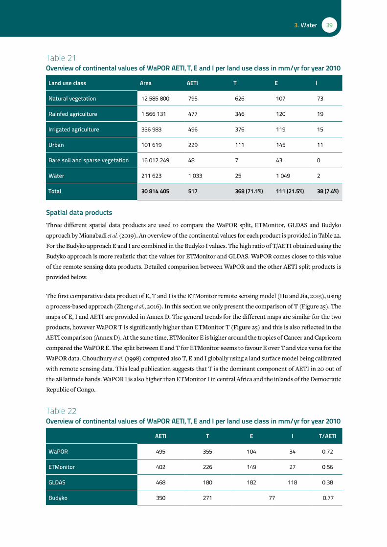
393. Water
Spatial data productsThree different spatial data products are used to compare the WaPOR split, ETMonitor, GLDAS and Budyko
approach by Mianabadi et al. (2019). An overview of the continental values for each product is provided in Table 22.
For the Budyko approach E and I are combined in the Budyko I values. The high ratio of T/AETI obtained using the
Budyko approach is more realistic that the values for ETMonitor and GLDAS. WaPOR comes closes to this value
of the remote sensing data products. Detailed comparison between WaPOR and the other AETI split products is
provided below.
The first comparative data product of E, T and I is the ETMonitor remote sensing model (Hu and Jia, 2015), using
a process-based approach (Zheng et al., 2016). In this section we only present the comparison of T (Figure 25). The
maps of E, I and AETI are provided in Annex D. The general trends for the different maps are similar for the two
products, however WaPOR T is significantly higher than ETMonitor T (Figure 25) and this is also reflected in the
AETI comparison (Annex D). At the same time, ETMonitor E is higher around the tropics of Cancer and Capricorn
compared the WaPOR E. The split between E and T for ETMonitor seems to favour E over T and vice versa for the
WaPOR data. Choudhury et al. (1998) computed also T, E and I globally using a land surface model being calibrated
with remote sensing data. This lead publication suggests that T is the dominant component of AETI in 20 out of
the 28 latitude bands. WaPOR I is also higher than ETMonitor I in central Africa and the inlands of the Democratic
Republic of Congo.
Table 21 Overview of continental values of WaPOR AETI, T, E and I per land use class in mm/yr for year 2010
Land use class Area AETI T E I
natural vegetation 12 585 800 795 626 107 73
rainfed agriculture 1 566 131 477 346 120 19
Irrigated agriculture 336 983 496 376 119 15
urban 101 619 229 111 145 11
bare soil and sparse vegetation 16 012 249 48 7 43 0
water 211 623 1 033 25 1 049 2
Total 30 814 405 517 368 (71.1%) 111 (21.5%) 38 (7.4%)
Table 22 Overview of continental values of WaPOR AETI, T, E and I per land use class in mm/yr for year 2010
AETI T E I T/AETI
wapor 495 355 104 34 0.72
etmonitor 402 226 149 27 0.56
gldAs 468 180 182 118 0.38
budyko 350 271 77 0.77

40 WaPOR quality assessment
The second remote sensing product to compare WaPOR T is the GLDAS T (Figure 26). Similar trends are found
between the two products, T for the rain forest in Congo are very similar, whereas the area around it shows large
deviations. In addition, GLDAS T is not able to capture the high T for irrigated areas (e.g. in the Nile Delta and
along the Nile River in Egypt), flood plains, shallow groundwater table areas and for deeper rooting groundwater
dependent ecosystems. The main reason is that the Land Surface Models of GLDAS consider rainfall as the only
source of water. Seepage, capillary rise, flooding and irrigation processes are still ignored in Land Surface Models.
GLDAS E is very similar to WaPOR E (see Annex D), however GLDAS I and WaPOR I differ significantly, with
GLDAS estimating very high I across the coastal areas in West Africa and generally between latitude of +10o to
–20o. GLDAS utilizes a canopy surface water storage (Rodell et al., 2004), this storage seems to be on the high side,
thereby overestimating I compared to WaPOR I.
Another just very recently published independent data source describing T comes from Mianabadi et al. (2019).
These authors used a well-known approach to separate T from I using the Budyko curve (Figure 27). Even though
the periods and the resolution differ (Budyko approach is an average over long time period for 0.25o), the values
are quite comparable. The Budyko method is overestimating T compared to WaPOR T in the Congo Basin, as well
as in the humid tropics of Ghana and Ivory Coast. The Budyko estimation of I, shows high values for areas in the
Lake Victoria basin in East Africa, and coastal zones such as the east coast of Madagascar and the coastal zones
in West Africa (see Annex D), which are also the same areas where WaPOR estimates very high PCP values. We
therefore believe that the larger picture of annual and absolute WaPOR T values for vast areas are good.
Mianabadi et al. (2019) compared their T and I products to two other products, GLEAM v3.0a (Martens et al., 2017;
Miralles et al., 2011a) and Simple Terrestrial Evaporation to Atmosphere Model (STEAM) (Wang-Erlandsson et al.,
2014, Wang-Erlandsson et al., 2016). The Budyko approach as presented here is in line with the two complex land
surface models (Mianabadi et al., 2019). WaPOR provides not only T and I values for each decade, it also provides
it at much higher resolution than the Budyko approach.
Figure 25 WaPOR and ETMonitor comparison of annual T values
etmonitor-wapor t (mm/yr)etmonitor t (mm/yr)0500100015002000
-1500-75007501500

413. Water
Figure 26 GLDAS T comparison with WaPOR T for the year 2010
Figure 27 Budyko T and comparison with WaPOR T
Field measurements of T fluxesA field site near Bir Marwa in the Takelsa Valley of northeast Tunisia (36.783055N, 10.624166E) was equipped
with sap flow instruments in a Michele Palieri table grape plantation during 2015 (Figure 28). Sap flow measures
directly the transpiration rate T, and is therefore a valuable asset for directly validating the T flux of WaPOR
without any indirect interpretations. The flow rates for each position are calculated as product of cross sectional
areas of the surrounding ring and the sap velocity (cm/hr). Measurements were taken at 15 min time interval and
gldAs - wapor t (mm/yr)-1000-50005001000
budyko - wapor t (mm/yr)-1000-50005001000
gldAs t (mm/yr)037575011251500
budyko t (mm/yr)037575011251500

42 WaPOR quality assessment
resulting sap flow is the sum of sap flow rates for inner and outer thermistors. The in situ measurements covers
the period May to December 2015.
The measured sapflow is approximately 1 mm/d during May when the LAI of the plantation is low (0.2 m2/m2).
The LAI increase to 1.5 m2/m2 by the end of June. The relatively low value of LAI is caused by the row crop charac-
ter of grapevines where the average LAI of canopies and underground reduces the total LAI for a field. The associ-
ated sapflow during the summer is typically 4 to 5 mm/d, a value that is according to the expectations, so there is
no doubt on the accuracy of the field measurements. At the end of December, the sapflow is again 1 mm/d, and it
expected to be even lower when the grapevines go dorment between December and May (Figure 29).
Figure 29 shows the disagreement with WaPOR T values. While at low T fluxes the performance of WaPOR is
at least realistic, the agreement disappears when the sapflow exceeds 2 mm/d. The T fluxes from WaPOR are in
general only 43 percent of the field measurements, hence a serious under-estimation in T is occuring. From the
entire period between 1 January 2009 and 11 January 2019, the maximum decadal T flux from WaPOR is 3.2 mm/d
only (October 2018). The maximum decadal AETI flux is 3.9 mm/d (August 2018). Clearly, peak T-fluxes are not
determined properly by WaPOR.
The accumulated T-flux from WaPOR for an average year is 503 mm/yr, the associated AETI-flux is 593 mm/
yr (hence T/AETI is 85% being a rather high value). The annual PCP is approximately 465 mm/yr. Indeed, the
grapevines are irrigated, and AETI values seem low. Hence, at local fields during the irrigation season, T values
from WaPOR are too low. The overall conclusion is that T from WaPOR is under-estimated at higher sapflow
values.
Figure 28 Location of the sap flow measurements in Tunisia

433. Water
B.3 ConclusionWith limited available data to compare E, T and I, we focused on comparing the WaPOR data with alternative
sources (ETMonitor, GLDAS, Budyko). All three T, E and I layers individually showed reasonable ranges in
values and spatial variability. Compared to ETMonitor, WaPOR estimates of T are more realistic. With limited
in situ observations available, the one comparison we did manage to do indicates that the T is underestimated
during the cropping season. For cropland with lower LAI (LAI~2), there are signals from the field scale analysis
that WaPOR T values are underestimated. Also, AETI was found to be at the lower side for several semi-arid and
arid test sites which can also be ascribed to low E values. Because LAI and rainfall have both distinct intra-annual
variabilities (that are not always related), it is recommended that T, E and I partitioning should be investigated
in more detail on a monthly basis.
The ETLook model applied in WaPOR separates the available energy into T and E depending on the factor α*LAI
(equation 7 and 8 in FAO, 2018), where α is the light extinction factor for net radiation [-] and LAI is the leaf
area index. As explained in FAO (2018), LAI is derived from a large number of similar functions compiled from
literature, however the value of α seems to be a calibration factor, which needs to be critically reviewed. Zhang
et al. (2014) identified different values for α based on a comprehensive analyses of different datasets. They found
variations between different land use classes and within land use classes (Table 23).
As the total bulk AETI is accurate (previous section), improving WaPOR T estimates can be achieved by refining
α, the sensitivity of this parameter should therefore be evaluated. If less available energy will go to T, then more
Figure 29 Measurement of actual transpiration fluxes with sapflow devices in a grape plantation in northeastern Tunisia

44 WaPOR quality assessment
will go to E for maintaining conservation of partition-
ing. That will immediately modify the T fraction in the
right direction. However, a warning should be given
that T should not be reduced much during full crop
development as various analyses suggested T to be at
the low side when crops are matured (Senegal, Sakha-A,
Zankalon, Jordan Valley). Again, more detailed analyses
are needed where the sensitivity to α is included for
assessing potential T fluxes, as well as the regulating
role of soil moisture on actual E and T fluxes. For now,
we conclude that T for most ecosystems is rather good
and in harmony with the most recent insights on T
fluxes, except for cropland where some improvements
are needed.
c. robustness C.1 IntroductionThe WaPOR water layers (AETI, T, E and I) and RET are calculated independently and at different resolutions
(250 m, 100 m or 30 m vs 20 km), comparing them therefore provides interesting validation of the WaPOR water
layers at continental scale. The coefficient between AETI and RET is also known as the crop coefficient (kc). The
coefficient is known to be high over water bodies, because there water is not a limiting factor. Over vegetated
areas, kc should reflect a curve depending on the crop stages during the growing season. The coefficient will be
low for bare land areas and similar dryland surfaces. A similar comparison was done to evaluate the ratio of T
over AETI, indicating the contribution of AETI towards biomass production (T) compared to non-productive
evaporation in the form of E and I. Low values of T/AETI are expected for water and bare soil, whereas for natural
vegetation and agriculture the values are expected in the range of 0.7 to 0.8.
For selected irrigation systems further analyses were done (see Figure 30 for locations of these irrigation
schemes). The Wonji irrigation scheme is located in Ethiopia in the Awash Basin and it is a sugarcane estate
in a semi-arid area. The Kpong irrigation schemes is located along the Lower Volta River in southern Ghana.
The Kpong includes mainly smallholders with rice, besides commercial farmers growing bananas. The area
has a humid climate. The Bekaa Valley is located in the Litani Basin in Lebanon, growing various crops, includ-
ing wheat, grapes and potatoes as well as other vegetables. The area is semi-arid. The forth area is the Fayoum
irrigation scheme in Egypt. The farmers of Fayoum grow maize (summer) and wheat (winter) on a rotational
basis. The irrigation schemes were selected based on the availability of auxiliary data and local knowledge of
the authors. IHE Delft has sent students for fieldwork to these regions as part of the WaPOR project. The MSc
thesis on the Wonji irrigation scheme was written by Yilma (2017). The MSc thesis dealing with the Bekaa Valley
was prepared by Alvarez-Carrion (2018). A study by Salvadore (2019) provided data for the Fayoum irrigation
scheme. The Kpong irrigation scheme in Ghana was added even though there was less data available, as it allowed
for a comparison of an irrigation scheme in a more humid climate.
Table 23 Light extinction factor for net radiation
Plant functional type/ land use class
αmean
grassland 0.50± 0.15
cropland 0.62± 0.17
shrubland 0.56± 0.13
broadleaf forest 0.59± 0.12
needleleaf forest 0.40± 0.11
Average 0.56± 0.16
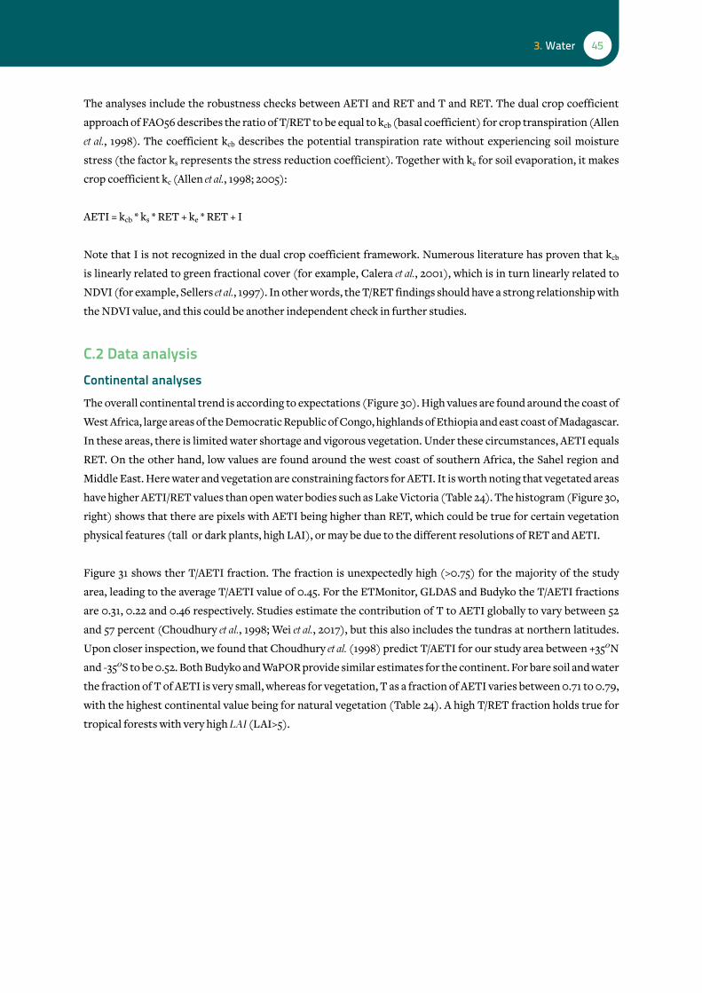
453. Water
The analyses include the robustness checks between AETI and RET and T and RET. The dual crop coefficient
approach of FAO56 describes the ratio of T/RET to be equal to kcb (basal coefficient) for crop transpiration (Allen
et al., 1998). The coefficient kcb describes the potential transpiration rate without experiencing soil moisture
stress (the factor ks represents the stress reduction coefficient). Together with ke for soil evaporation, it makes
crop coefficient kc (Allen et al., 1998; 2005):
AETI = kcb * ks * RET + ke * RET + I
Note that I is not recognized in the dual crop coefficient framework. Numerous literature has proven that kcb
is linearly related to green fractional cover (for example, Calera et al., 2001), which is in turn linearly related to
NDVI (for example, Sellers et al., 1997). In other words, the T/RET findings should have a strong relationship with
the NDVI value, and this could be another independent check in further studies.
C.2 Data analysisContinental analysesThe overall continental trend is according to expectations (Figure 30). High values are found around the coast of
West Africa, large areas of the Democratic Republic of Congo, highlands of Ethiopia and east coast of Madagascar.
In these areas, there is limited water shortage and vigorous vegetation. Under these circumstances, AETI equals
RET. On the other hand, low values are found around the west coast of southern Africa, the Sahel region and
Middle East. Here water and vegetation are constraining factors for AETI. It is worth noting that vegetated areas
have higher AETI/RET values than open water bodies such as Lake Victoria (Table 24). The histogram (Figure 30,
right) shows that there are pixels with AETI being higher than RET, which could be true for certain vegetation
physical features (tall or dark plants, high LAI), or may be due to the different resolutions of RET and AETI.
Figure 31 shows ther T/AETI fraction. The fraction is unexpectedly high (>0.75) for the majority of the study
area, leading to the average T/AETI value of 0.45. For the ETMonitor, GLDAS and Budyko the T/AETI fractions
are 0.31, 0.22 and 0.46 respectively. Studies estimate the contribution of T to AETI globally to vary between 52
and 57 percent (Choudhury et al., 1998; Wei et al., 2017), but this also includes the tundras at northern latitudes.
Upon closer inspection, we found that Choudhury et al. (1998) predict T/AETI for our study area between +35οN
and -35οS to be 0.52. Both Budyko and WaPOR provide similar estimates for the continent. For bare soil and water
the fraction of T of AETI is very small, whereas for vegetation, T as a fraction of AETI varies between 0.71 to 0.79,
with the highest continental value being for natural vegetation (Table 24). A high T/RET fraction holds true for
tropical forests with very high LAI (LAI>5).

46 WaPOR quality assessment
Figure 30 Average WaPOR AETI over RET (2009-2017), with locations of selected irrigation schemes (next section)
Table 24 Overview of continental values of WaPOR robustness
Land use class Area AETI T RET AETI/RET T/AETI T/RET
natural vegetation 12 585 800 795 626 1 412 0.56 0.79 0.44
rainfed agriculture 1 566 131 477 346 1 484 0.32 0.73 0.23
Irrigated agriculture 336 983 496 376 1 556 0.32 0.76 0.24
urban 101 619 229 111 1 699 0.13 0.49 0.07
bare soil and sparse vegetation
16 012 249 48 7 2 036 0.02 0.14 0.00
water 211 623 1 033 25 1 490 0.69 0.02 0.02
Total 30 814 405 503 368 1 742 0.22 0.73 0.16
Irrigation scheme comparisonFigure 32 overleaf shows the AETI/RET ratio (i.e. kc) and on the right the T/RET ratio (i.e. kcb) for the selected
irrigation schemes for one calendar year (2015). Except for the area in Ghana, the maps clearly show the distinc-
tion between the irrigated and surrounding landscapes. In Wonji, Fayoum and Bekaa, the surrounding area is
water constrained. The availability of water is clearly a distinguishing factor in the development of vegetation.
For the area in southern Ghana, the irrigated area cannot be distinguished as easily as in the arid and semi-arid
areas.
freq
uenc
y
140000
120000
100000
80000
60000
40000
20000
00 0.5
pixel value
raster histogram
1 1.5
wapor AetI/ret00.250.50.751

473. Water
Figure 31 Fraction of T over AETI (2009-2017)
The average AETI, T, E and I for
the selected irrigation schemes are
provided in Table 25. Since the anal-
yses include not only the cropping
season, fallow periods will reduce
kc and the period of fully developed
crops will increase the average
kc value. Because sugarcane is a
perennial crop, it produces much
higher kc value (0.67) than what
is observed for Fayoum (0.22) and
Bekaa (0.5) exhibiting crop rota-
tion systems (Table 25). In addi-
tion, for the Fayoum system, not
all fields are cultivated with wheat
during the winter season, as indi-
cated in the blue areas (Salvadore,
2019). The bright red area in the
Fayoum system is the Qarun Lake,
where Kc is close to 1. The produc-
tive component of AETI (T) varies per irrigation scheme. Fayoum in Egypt has the lowest value of productive
AETI of 0.69 and Wonji the highest of 0.85 (Table 25).
The basal crop coefficient (kcb) of the selected irrigation schemes ranges between 0.15 for the Fayoum system to
0.57 for Wonji. The season variation of AETI/RET and T/RET are presented in Figure 33 and 34. The theoretical kc
of sugar cane is 1.25 (Allen et al., 1998) however, based on the WaPOR data, the annual kc value for Wonji is much
lower at 0.67. This value is lower than the theoretical one, as various areas within the defined shapefile are not
cropped, either they are fallow or consist of paths, buildings etc.
Table 25 Overview of WaPOR AETI, T, E and I per selected irrigation scheme for 2015
Name Country Main crop type AETI T E I kc (AETI/RET)
T/AETI kcb (T/RET)
wonji Ethiopia Sugarcane 1,317 1,125 182 18 0.67 0.85 0.57
fayoum Egypt Wheat, maize* 485 333 153 0 0.22 0.69 0.15
bekaa Lebanon Wheat, potatoes, grapes
622 494 131 6 0.50 0.79 0.40
kpong Ghana Rice 1,196 875 302 30 0.75 0.73 0.55
Bananas 1,022 793 201 40 0.63 0.78 0.49
* rotational cropping
wapor t/AetI (-)00.250.50.751

48 WaPOR quality assessment
Figure 32 The AETI/RET ratio (left) and T/RET ratio (right) for selected irrigation schemes for year 2015 (from top to bottom: Wonji - Level 3, Fayoum - Level 2, Bekaa - Level 3, Kpong - Level 2)

493. Water
Figure 33 Monthly AETI/RET ratio for selected irrigation schemes
Figure 34 Monthly T/RET ratio for selected irrigation schemes
0
0.2
0.4
0.6
0.8
1
1.2
AETI
/RET
(kc)
Jan
Wonji-sugar cane Bekaa Kpong-rice Kpong-banana
Feb Mar Apr May Jun Jul Aug Sep Oct Nov Dec
0
0.2
0.4
0.6
0.8
1
1.2
T/RE
T (k
cb)
Jan
Wonji-sugar cane Bekaa Kpong-rice Kpong-banana
Feb Mar Apr May Jun Jul Aug Sep Oct Nov Dec

50 WaPOR quality assessment
C.3 ConclusionWaPOR AETI/RET ratio (kc) at continental scale is 0.22, which at first glance seems low, but includes large areas
in the Sahara and the Sahel regions where little or no evaporation is taking place. WaPOR AETI/RET ratio for the
different land use classes confirms the accuracy of the WaPOR AETI layer compared to WaPOR RET, where high
values are obtained in densely vegetated areas and for water bodies. WaPOR T/RET ratio (kcb) at continental scale
is 0.16, with higher values for vegetated areas (agriculture and natural vegetation) and low values for bare soil
and water. Similarly, WaPOR T/AETI ratio at the continental scale exceeds 0.7. These high T/AETI fractions are
supported by the Budyko analysis (Mianabadi et al., 2019), and they are certainly reasonable for permanently lush
green ecosystems. The general trends are consistent with expected values.
At irrigation system level, the comparative analyses show lower value for the AETI/RET and T/RET for the
Fayoum and Bekaa irrigation schemes than expected for cropped areas. This could be due to parts of the area
being fallow (e.g. Fayoum), or parts of the year being fallow, thereby lowering the ratios. The schemes in Ghana
and Ethiopia are cropped for most of the year and return values that are more in the expected range for cropped
areas. In these areas, productive evaporation (T) is significantly higher than unproductive evaporation (E and I).
For systems with a significant fallow area (Fayoum), the T/AETI ratio is low.
To confirm the accuracy of the values additional comparison with NDVI is necessary (NDVI at the moment is not
available from WaPOR). One issue of concern is that T/AETI fractions vary strongly with LAI, PCP and the soil
moisture regulation of E and T fluxes. The underlaying processes can be judged much better if in the next round
of quality assesment decadal values are going to be investigated. Hence, it is not unlikely that WaPOR T provides
some new evidence that T/AETI should be higher than previously assumed.

513. Water
Det
ail o
f WaP
OR
Map
“A
bove
Gro
und
Bio
mas
s P
rodu
ctio
n 20
18 -
Eas
tern
Ang
ola
and
Wes
tern
Zam
bia”
4. Land
A. Above Ground Biomass Production A.1 IntroductionProducing more food per unit of land (kg/ha) and per unit of water (kg/m3) is a major objective for increasing
sustainable production in agriculture. FAO has shown in various studies that more food needs to be produced
for meeting growing global food demand, and that will increase pressure on water resources. Most global data on
crop yield and water resources are based on FAOSTAT and AQUASTAT. This data is based on secondary statistical
datasets from the member countries. FAO launched the WaPOR program to complement such statisticswith
spatially distributed information a on the local variability and trends in time, using cost-effective technologies.
The Above Ground Biomass Production (AGBP) is the ultimate indicator to express food production. The
WaPOR database contains information on Above Ground Biomass Production (AGBP) based on the Net Primary
Production (NPP). NPP reflect the daily net carbon exchange between land and atmosphere. During sunlight
hours, crops intake carbon along with the release of water vapor into the atmosphere. During nighttime, part of
the carbon is respired back into the atmosphere. The net result is the NPP. NPP is calculated in WaPOR using a
remote sensing light use efficiency model (Ruimy et al., 1999). NPP is expressed in gC/m2/day. It is converted from
gC to kg of dry mass (DM) per ha using a conversion factor of 22.22 (FAO, 2018). An additional conversion factor

52 WaPOR quality assessment
to account for the percentage of biomass produced above ground is introduced. This conversion factor expresses
the total weight of stems, branches, leaves, flowers, grains and lints above ground, versus the total weights of
stubbles, bulbs, roots and tubers. In WaPOR, an average factor of 0.65 is applied throughout all pixels across
the continent (FAO, 2018). The calculated continental AGBP considers C3 crop types and currently doesn’t
account for variations in land use and crop types to adjust the fraction of AGBP to total biomass and correct for
different crop types. The database provides data on AGBP, which makes sense for cereals and most other crops.
For potatoes, sugar beet and other tuber, root and bulb crops, it is better to revert back to the Total Biomass
Production (TBP). This can be achieved as TBP = AGBP/0.65.
These constant factors are described in the methodology (FAO, 2018) but the implications associated with the
simplifications should be well explained to users of the WaPOR database and instructions given on how to correct
them when using the WaPOR database. For example, the ratio of the above and below ground biomass production
varies across landscapes, and if users have (literature) information on this shoot – root ratio, a correction can be
easily made. It should be made clearer to users that the default shoot – root ratio is 0.65.
C4 crops have a different biochemical system that converts the available solar radiation with a higher light use
efficiency into dry matter or biomass production. On average, their extra efficiency is 80 percent higher as
compared to C3 crops (being most crops). The most common C4 crops are sugarcane, maize and various oil
seeds. To be able to estimate biomass and yield correctly for C4 crops, the WaPOR data thus needs to be corrected
for areas where these crops grow.
A.2 Data analysisThe average WaPOR AGBP and NPP values for 2009-2017 are presented in Table 26 and Figure 35. As AGBP is
linearly related to NPP, the two maps show the same variation across the continent. Variations between years at
the continental scale are very small. The continental map is dominated by the close to zero values in the Sahel
and large part of the Middle East. Larger inter-annual variations exist in the areas dominated by rainfall. In both
maps, irrigated areas around the Nile river (Egypt) and the Office du Niger and Inner Niger Delta (Mali) appear
clearly as bright spots in otherwise dry, low biomass producing areas.
Spatial data productsTo the authors knowledge, only one comparative remote sensing product of NPP exists with a similar grid size
(MOD17) (Heinsch et al., 2003; Running and Zhao, 2015; Running et al., 2015), besides several other assessments
from global ecological production models. For this assessment a comparison is made with the MOD17 Terra
and Aqua NPP products. There are discrepancies between the MOD17 Aqua and Terra products resulting from
differences in overpass time, therefore we compared WaPOR NPP with the averages of the MODIS Terra and
Aqua NPP products for 2011 (Figure 36).
The spatial patterns are similar for both data products even though MODIS does not estimate values for the Sahel
region. The absolute difference between the two products shows large discrepancies between the two products
in the Central African Republic (underestimation of MODIS compared to WaPOR), whereas the eastern part of
Southern Africa and eastern Madagascar is generally overestimated by MODIS (Figure 37).

534. Land
Table 26 Average continental values of WaPOR ABGP and NPP
2009 2010 2011 2012 2013 2014 2015 2016 2017 Average
npp in kgc/m2/yr
max 1.42 1.41 1.48 1.54 1.61 1.65 1.61 1.60 1.49 1.53
mean 0.20 0.19 0.21 0.20 0.17 0.19 0.17 0.17 0.20 0.19
min 0 0 0 0 0 0 0 0 0 0
stdev 0.63 0.63 0.64 0.63 0.62 0.63 0.63 0.63 0.64 0.51
Agbp in tonnes/ha/yr
max 27.3 26.7 26.6 28.4 24.2 27.4 27.8 27.0 26.9 26.9
mean 4.6 4.6 4.7 4.7 4.7 4.6 4.5 4.4 4.5 4.6
min 0 0 0 0 0 0 0 0 0 0
stdev 5.6 5.6 5.6 5.7 5.7 5.7 5.7 5.6 5.6 5.6
Figure 35 Annual Above Ground Biomass Production (AGBP) and Net Primary Production (NPP) values averaged for 2009-2017 period
wapor Agbp (kg/ha)
06250125001875025000
wapor npp (kgc/m2)
00.350.71.051.4

54 WaPOR quality assessment
Figure 36 WaPOR NPP and average of MODIS Terra and Aqua NPP for 2011 (kgC/m2)
Figure 37 Difference NPP WaPOR and MODISAv as a fraction of MODISAv (left) and as absolute value (right) for 2011
Even though it is difficult to say which data layer provides better NPP quality, the AETI comparison showed that
WaPOR comes out with much better quality product than the MOD16 AETI product. Both products are using
light use efficiency based approaches, but the choice of parameters, especially light use efficiency can create large
deviations in the products.
Another independent check can be achieved from comparisons against global ecological production models.
Figure 38 shows the result of NPP simulations done by the Center of Sustainability and the Global Environment
wapor npp (kgc/m2)
00.350.71.051.4
modIs npp (kgc/m2)
00.3650.731.091.46
(wapor-modIs npp modIs npp (-)
-1-0.500.51
(wapor-modIs npp (kgc/m2)
-1-0.500.51

554. Land
under the aegis of the University of Wisconsin. This IBIS model8 shows NPP to vary between 0 and 1.3 kg C/m2/
yr (Foley et al., 2005; Kucharik et al., 2000). The spatial trend for Africa is rather similar to WaPOR NPP, but with
much lower resolution. Clearly, WaPOR NPP is able to differentiate water bodies and irrigated areas much better
than the IBIS model (Figure 38).
WaPOR NPP is derived using light use efficiency value for different land use classes, for cropped areas it applies
one value of 2.49 MJ/gr across the continent (FAO, 2018). This value corresponds to above and below ground
biomass production (total biomass production (TBP)) and C3 crops. The light use efficiency values applied for
trees, savannah and pastures are not provided in FAO (2018) and should be lower than for C3 crops (Foley et al.,
2005; Madini et al., 2017). More information should be provided on the light use efficiency applied for the various
agro-ecosystems and compared to other literature (e.g. Li et al., 2012; Madani et al., 2017).
Biomass estimates for selected irrigation schemesPoint measurements of AGBP are classically validated using crop yield data, which involve crop specific conver-
sion parameters (harvest index, moisture content in the harvested fresh crop). A comparison was made to evalu-
ate biomass production and yield to known values for the four selected irrigation schemes. For Wonji and Bekaa
Valley, Yilma (2017) and Alvarez-Carrion (2018) used the pySEBAL script developed by IHE Delft and collected
field data from the two areas. For Fayoum, Salvadore (2019) worked with the Ministry of Water and Irrigation in
Egypt to develop a water account for the area, this included validation data on yield. For the area in Ghana, two
reports from the Ghana Irrigation Development Authority were used to validate the results (GIDA, 2010). These
datasets were used to compare the WaPOR AGBP layer. The total biomass production (TBP) was derived from
NPP using the same conversion factors as the WaPOR database, without using the ratio of 0.65 of above ground
8 https://daac.ornl.gov/cgi-bin/dsviewer.pl?ds_id=808
Figure 38 Global and annual NPP values simulated with the IBIS model (Foley et al., 2005) and difference with WaPOR NPP
Figure 38 Global and annual NPP values simulated with the IBIS model (Foley et al., 2005) and difference with WaPOR NPP
IbIs - wapor npp (kgc/m2)
-1-0.500.51
IbIs npp (kgc/m2)
00.350.71.051.4

56 WaPOR quality assessment
biomass production over total biomass production (FAO, 2018). The crop yield (Y) was then multiplied by a
harvest index (hi), for C4 crops multiplied by a factor of 1.8 (C4). The final conversion is dividing by one minus the
moisture content of the crop yield (mc):
TBP * hi * C 4
The harvest index and moisture content are crop (and location) specific parameters. For Bekaa and Wonji the
WaPOR Level 3 (30 m resolution) is available, whereas for Fayoum and Kpong the 100 m resolution data was used.
Wonji irrigation scheme
The Wonji irrigation scheme is located in the Awash Basin, the area selected for comparison is an area cultivated
with sugarcane. The cropping season of sugar cane in this area is 12-24 months on a rotational basis. We compared
WaPOR yield to the yield observations, taking into account that the cropping season extends beyond one year.
Even though, the AGBP layer for 30 m from the WaPOR portal is compiled based on the WaPOR determined
cropping season (see section C), we decided to use our own predefined cropping season. We decided to estimate
annual values for AGBP from January 2015 to June 2016 (18 months crop rotation), which is a similar period as
Yilma (2017) used for the pySEBAL analyses.
WaPOR AGBP was converted back to Total Biomass Production (TBP) by dividing it by 0.65 (the ratio used by
WaPOR). This TBP was multiplied by a crop specific ratio of AGBP and TBP (in this case set at 1.0 as root devel-
opment for rotational sugar cane was assumed to be low). This was then multiplied by a harvest index (for sugar
cane this was set at 1.0 as all harvested sugar cane ends up at the factory)9. An additional conversion was made to
convert from C3 to C4 crops (factor 1.8). Finally the dry yield was converted to wet yield by dividing the value by
the moisture content of the crop (set at 0.59, as estimated by Yilma (2017)).
Figure 39 and 40 show the maps of AGBP and yield for the area (the whole map was converted using the
conversion factors as describe before).
Figure 41 show the yield distribution within the Wonji irrigation scheme. The average yield for 2015 a calculated
is 100 tonnes/ha (Table 27). This value is similar to Yilma (2017) observed of 100 tonnes/ha. Steduto et al (2012)
gives an average cane yield of 70 tonnes/ha and FAO gives ranges between 50-150 tonnes/ha being in perfect
agreement with our check. Hence, WaPOR yield based on WaPOR AGBP seems rather realistic for sugarcane
crops.
9 Note that this harvest index is higher than reported in literature (0.65-0.85) and 0.65 estimated by Yilma (2017)
1 - mcY=

574. Land
Figure 39 WaPOR Above Ground Biomass Production for 2015 for the Wonji irrigation scheme
Figure 40 WaPOR derived yield for 2015 for the Wonji irrigation scheme using AGBP and specific conversion factors for sugarcane

58 WaPOR quality assessment
Figure 41 Sugarcane yield distribution Wonji irrigation scheme
0 5 10 15 20 25 30 35 40 45 50 55 60 65 70 75 80 85 90 95 100
105
110
115
120
125
130
135
140
145
0
20
40
60
80
100
120
140
160
180
Yield (tonnes/ha)
Table 27 WaPOR yield estimates for Kpong irrigation scheme for the year 2015
Crop User defined cropping season Harvest index
Moisture content
Average yield (tonnes/ha)
Literature values (tonnes/ha)
sugarcane 01/01/2015-30/06/2016 1.0 0.59 100 100
Bekaa Valley irrigationThe Bekaa Valley is located in the Litani Basin in Lebanon. The farmers are growing a variety of crops, we obtained
a shapefile of some grape fields (Alvarez-Carrion, 2018) and used this for the analyses. Figure 42 presents the
AGBP in the area for the year 2015. The small shapes (southeast of the Bekaa Valley) are the known areas where
table grapes are grown (Alvarez-Carrion, 2018).
The WaPOR yield estimation for this small area used the harvest index and moisture content as indicated in Table
28. Using these parameters the estimated yield for the grapes in these areas is 7.6 tonnes/ha, which is very close to
the reported yield of 7.5 tonnes/ha (Alvarez-Carrion, 2018). The yield varied between 3.5 and 11 tonnes/ha (Figure
43). So also here, AGBP and TGBP values are accurate, but crop yield can be assessed only with proper Harvest
Index and moisture content values of the fresh product.
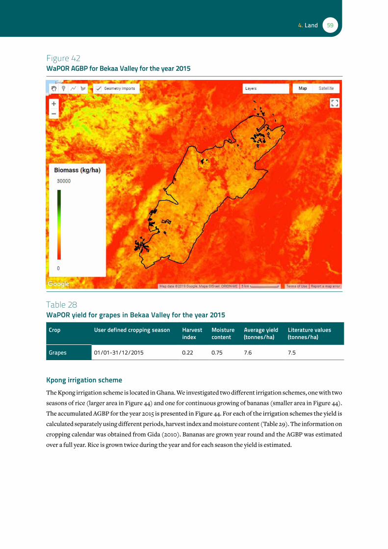
594. Land
Table 28 WaPOR yield for grapes in Bekaa Valley for the year 2015
Crop User defined cropping season Harvest index
Moisture content
Average yield (tonnes/ha)
Literature values (tonnes/ha)
grapes 01/01-31/12/2015 0.22 0.75 7.6 7.5
Figure 42 WaPOR AGBP for Bekaa Valley for the year 2015
Kpong irrigation schemeThe Kpong irrigation scheme is located in Ghana. We investigated two different irrigation schemes, one with two
seasons of rice (larger area in Figure 44) and one for continuous growing of bananas (smaller area in Figure 44).
The accumulated AGBP for the year 2015 is presented in Figure 44. For each of the irrigation schemes the yield is
calculated separately using different periods, harvest index and moisture content (Table 29). The information on
cropping calendar was obtained from Gida (2010). Bananas are grown year round and the AGBP was estimated
over a full year. Rice is grown twice during the year and for each season the yield is estimated.

60 WaPOR quality assessment
Figure 43 Yield distribution of grapes in Bekaa Valley for the year 2015
Bekaa grapes
0
2
4
6
8
10
12
14
Yield (tonnes/ha)
Freq
uenc
y
0
0.5 1
1.5 2
2.5 3
3.5 4
4.5 5
5.5 6
6.5 7
7.5 8
8.5 9
9.5 10
10.5 11
11.5 12
12.5 13
13.5 14
14.5
Figure 44 WaPOR AGBP at Kpong irrigation scheme for the year 2015
Figure 45 shows the WaPOR estimated yield for bananas. In this humid climate it is difficult to distinguish
between the natural vegetation and the irrigated and or agricultural areas. Table 29 shows the estimated yield
which compares very well with the reported yield by Gida (2010).
biomass (kg/ha)30000
0

614. Land
Figure 45 WaPOR yield estimation for banana plantation at Kpong irrigation scheme for the year 2015
Table 29 WaPOR yield estimates for Kpong irrigation scheme for the year 2015
Crop User defined cropping season Harvest index
Moisture content
Average yield (tonnes/ha)
Literature values (tonnes/ha)
bananas 01/01-31/12/2015 0.6 0.76 37.6 40
rice main season
01/03-31/07/2015 0.55 0.2 4.2 4-5
rice minor season
01/08-31/12/2015 0.55 0.2 4.0 4-5

62 WaPOR quality assessment
Figure 46 Distribution of WaPOR estimated yield for Kpong irrigation scheme for the year 2015
Kpong rice s1
0 1 2 3 4 5 6
Kpong rice s2
0 10 20 30 40 50 60
Kpong banana s1
0
5
10
15
20
25
30
35
40
0
10
20
30
40
50
60
70
Freq
uenc
yFr
eque
ncy
0
10
20
30
40
50
60
70
80
Freq
uenc
y
Yield (tonnes/ha)
Yield (tonnes/ha)
0 1 2 3 4 5 6
Yield (tonnes/ha)

634. Land
Fayoum irrigation schemeThe Fayoum irrigation scheme is divided in two areas, one with permanent tree crops in orchards and an area
where wheat and maize are grown on a rotational basis. The area receives very little rainfall, and most AGBP
occurs on irrigated fields (Figure 47).
Yield is estimated using the cropping season as defined by Salvadore (2019). The harvest index and moisture
content for each crop are presented in Table 30, and the estimated yield presented in Figure 48. The estimated
yield for wheat and oranges are in the right ballpark, the estimated yield for maize is a bit on the low side (Table
30). The yield distribution (Figure 49) shows a large variation, and could be attributed to non-uniform water
distribution, soil salinity and variable depth to shallow water table (see the red areas on Figure 48), which lower
the yields. While wheat is the dominant winter crop, maize is cultivated side by side with berseem (and rice)
during the summer. This quick analysis show the importance of having crop maps available. The user community
of WaPOR should get examples on how to prepare their own crop masks, and then superimpose on WaPOR AGBP.
A.3 ConclusionsThe WaPOR NPP layer is computed using a light use efficiency methodology. The maximum light use efficiency
differs for different biomes and crop types, meaning that an accurate land use map is required to assign the
correct values for each land use type. Correction factors for ambient conditions and soil moisture are included
Figure 47 WaPOR AGBP at Fayoum for the year 2015

64 WaPOR quality assessment
Figure 48 WaPOR derived yield for wheat (November 2015- May 2016) and maize (June-October 2016)
Table 30 Crop productivity Fayoum system
Crop Cropping period Harvest index
Moisture content
Average yield (tonnes/ha)
Literature values (tonnes/ha)*
wheat (c3) 01/11/2015-31/05/2016 0.45 0.15 5.3 5
maize (c4) 01/06/2016-31/10/2016 0.45 0.26 3.1 4.4
oranges 01/01/2015-31/12/2015 0.22 0.85 17.7 20
* salvadore, 2019

654. Land
Figure 49 WaPOR yield distribution for wheat, maize and oranges in Fayoum irrigation scheme for the year 2015
Fayoum wheat
0 1 2 3 4 5 6 70
200
400
600
800
1000
Freq
uenc
y
Yield (tonnes/ha)
0 1 2 3 4 5 6
Fayoum maize
Orange
1 2 3 4 5 6 7 8 9 10 11 12 13 14 15 16 17 18 19 20 21 22 23 240
50
100
150
200
250
300
Freq
uenc
y
0
200
400
600
800
1000
1200
1400
Freq
uenc
y
Yield (tonnes/ha)
Yield (tonnes/ha)

66 WaPOR quality assessment
in WaPOR (FAO, 2018). NPP appears to lay in the same range for the NPP product based on MODIS images
(MOD17), however there are also substantial differences between the two products. From this comparison, we
cannot conclude that one of the products produces more realistic values that the other. However from the AETI
comparison, WaPOR was much more accurate, and we therefore conclude that the differences observed do not
necessarily mean WaPOR NPP and derived WaPOR AGBP layer is inaccurate.
The analyses show that the WaPOR AGBP layers are excellent proxies for crop yield, if the WaPOR database
users have the proper skills to interpret the data. As there is a large range for total to above ground biomass
production between different crop types, the first step is to revert to Total Biomass Production (TBP). The
second consideration is that time integrated values of AGBP are required following the cropping season. The
third one is that every crop has specific ranges of harvest index and moisture of the fresh harvestable product
that need to be applied. These values require actually some local tuning. The last point is that C4 crops require an
incremental TBP due to the fact that they are more efficient with solar light.
Yet, we demonstrate here examples from the Wonji sugarcane irrigation scheme in the Awash Basin that AGBP
is a proxy for fresh yield. The conversion from AGBP to yield included conversion from AGBP back to TBP, crop
specific ratio of ABGP over TBP, crop specific harvest index, C3 to C4 crop conversion, and moisture content of
the crop. With these conversion factors, the estimation of yield for sugarcane in Wonji is within the expected
range and in line with observed yield. Similar analyses for grapes in the Bekaa Valley, rice and bananas in Kpong
irrigation scheme and wheat, maize and oranges in Fayoum give good results. It must be said that each conver-
sion factor adds additional uncertainty to the yield estimations, but that the availability of WaPOR AGBP data
with ten days intervals provides a solid fundament for any crop yield estimation process. You cannot estimate
crop yield without spatiotemporal information on AGBP or TBP. It is the first time that such data is now available
for the African continent for a period of ten years.
For the irrigation schemes located in the arid to semi-arid zones, agricultural lands can be clearly distinguished
from the surrounding natural vegetation. The case studies in Ghana and Lebanon give good yield estimations,
however the surrounding natural landscape reflects in similar fashion. However, total biomass production can
be significantly under or over-estimated when the agricultural lands are not clearly defined.
b. land cover classificationB.1 IntroductionThe WaPOR Land Cover Classification (LCC) layer has different levels of detail for the different scales. At 250
m resolution, the WaPOR LCC has six land cover classes (natural vegetation, rainfed agriculture, irrigated agri-
culture, urban, bare soils and water). On the 100 m resolution, there are ten land cover classes, namely natural
vegetation is split into tree cover, shrubland, grassland and wetland, whereas water is split into permanent and
seasonal. At 30 m resolution, more detail of crop types are added for both rainfed and irrigated agriculture. The
WaPOR LCC layer is based on NDVI and phenology and is generated using machine learning (FAO, 2018).

674. Land
B.2 Data analysesDatabase comparisonsThe main application of the WaPOR database is agricultural productivity. Therefore, the identification of
rainfed and irrigated agricultural areas are most important. Two datasets were used for comparison, the FAO
based Global Map of Irrigated Area (GMIA) is part of the FAO AQUASTAT database (FAO, 2016) and the Global
Irrigated Area Map (GIAM) (Dheeravath et al., 2010). The GMIA includes sub-national irrigation statistics for
most countries. The target year for the statistics is the year 2005. The spatial resolution of the map is 5 minutes.
The information listed per country is a compilation of literature review and secondary data. The GIAM is an
alternative spatial database developed by the International Water Management Institute (IWMI) using remote
sensing data (http://waterdata.iwmi.org/applications/irri_area/), whereas GMIA database is a database compiled
of national level data. GMIA is based on official statistics that are recognized by countries in spite of the lack
of update through the statistical means10. The comparisons of WaPOR LCC (Level 2) for 18 countries against
GMIA, and GIAM are summarized in Table 31. The three datasets do not have exactly same definitions in irrigated
areas, but the direct comparison gives an indication of variations among the three sources.
10 http://www.fao.org/nr/water/aquastat/irrigationmap/index20.stm
Table 31 Rainfed and irrigated areas from WaPOR (2014), FAO AQUASTAT (2013-7) and GIAM (2010)
Rainfed areas (ha) Irrigated areas (ha)
WaPOR GMIA GIAM WaPOR GMIA* GIAM
benin 2 546 895 3 176 960 2 181 150 259 350 23 040 49 929
ethiopia 18 398 918 15 400 700 21 381 713 872 852 858 300 2 247 969
egypt 893 590 135 000 687 281 3 370 265 3 610 000 3 206 476
ghana 2 100 164 7 400 000 4 371 500 203 445 30 900** 607 783
mozambique 4 519 522 5 831 900 2 648 650 715 930 118 100 374 938
Jordan 691 069 218 600 360 256 47 872 103 400 92 006
kenya 4 786 339 6 179 400 4 202 725 1 235 227 150 600 1 970 415
lebanon 495 938 258 000 244 538 45 598 104 000** 250 831
morocco 10 731 604 8 072 000 4 323 838 655 903 1 520 000 2 124 749
mali 6 263 474 6 189 900 8 364 825 2 208 640 371 100 273 489
occupied palestinian territory 402 615 148 000 13 474 24 000**
republic of south sudan 1 102 896 2 721 900 3 757 100 141 527 38 100 31 637
syria 6 284 334 4 392 000 2 458 456 429 646 1 341 000 1 125 514
tunisia 5 128 812 4 745 400 488 638 159 046 486 600 1 701 626
uganda 5 176 311 9 088 860 8 304 775 472 430 11 140 1 352 538
yemen 164 884 1 546 000 2 546 863 627 716 454 300** 851 063
Total 69 687 365 75 504 620 66 322 308 11 458 921 8 631 380 16 260 963
* definition in AQuAstAt: Area equipped for irrigation - total
** fAo AQuAstAt statistics available before 2013

68 WaPOR quality assessment
Overall, it is difficult to draw conclusive observations from the comparisons, except that WaPOR lies in between
GMIA and GIAM. GMIA data originates mostly from country reporting system and suffer from varying qualities
in the process. GIAM on the other hand was produce
Correlation analysis in Figure 50 shows that overall WaPOR overestimated rainfed areas compared to both
GMIA and GIAM. WaPOR estimated much larger rainfed areas for Morocco, occupied territories of Palestine,
Syria and Tunisia. However in Ghana and Yemen, WaPOR underestimates rainfed areas compared to the other
two sources. The irrigated areas of the three sources show larger variations among each other. Overall WaPOR
values tend to be smaller or significantly smaller than the GIAM database. One key outlier is Mali, where WaPOR
reported 2.2 million ha of irrigation while the other two sources reported 0.27 to 0.38 million ha only. For Mali,
large parts of the Inner Niger Delta are classified as irrigated areas, in GMIA, these areas are likely reported under
agricultural water management areas, which include wetlands and flood recession agriculture. The total area
for this class in Mali in GMIA is 621 000ha, which is still well below the WaPOR estimates. Excluding Mali, for
the remaining 11 countries where all three sources have data, the total irrigated areas reported by WaPOR is 101
percent of GMIA data on “Total area equipped for irrigation” but 59 percent of GIAM. GMIA is based on official
national statistics and not updated regularly, it therefore does not always capture recent development in irriga-
tion in Africa hence have a tendency to under report. Since the WaPOR LCC is reporting similar areas, it is there-
fore also under estimating the irrigated areas. WaPOR LCC for Ethiopia and Kenya suggest an area of 2.2 million
ha, and this is a rather large discrepancy that can be associated to definitions and other factors. Nevertheless, it
confirms that the WaPOR LCC seriously underestimates irrigated areas.
Comparison land use maps WA+ basinsAs part of the FAO WaPOR project, IHE Delft is implementing Water Accounting studies for five river basins,
Litani, Jordan, Awash, Nile and Niger. For the Water Accounting studies, a detailed land use map is required. A
consultant was hired to develop detailed land use maps using a novel machine learning approach (Saah et al., in
preparation). It uses similar algorithms to WaPOR, such as the random forest regression method. For the land
use classifications, reference data were collected from high resolution satellite imagery. Points were collected in
Figure 50 Comparisons of rainfed and irrigated areas in 18 countries from WaPOR, GMIA, and GIAM
rainfed areas Irrigated areas
Inde
pend
ent d
ata
set e
stim
ate
(ha)
Inde
pend
ent d
ata
set e
stim
ate
(ha)
wapor estimate (ha) wapor estimate (ha)
0 05,000,000 1,000,00010,000,000 2,000,00015,000,000 3,000,00020,000,000 4,000,00025,000,000 5,000,000
25,000,000
20,000,000
15,000,000
10,000,000
5,000,000
0
5,000,000
4,000,000
3,000,000
2,000,000
1,000,000
0
0

694. Land
the categories water, barren, urban, field crops, tree crops, grass, forest, shrub and snow. High resolution earth
observation data allowed to select locations with extended coverage of one particular class without spectral
mixing from other classes. All points were sampled in one dataset (Poortinga et al. in prep. a&b). The resulting
land use classification follows the Water Accounting Plus classification, differentiating between natural and
managed land use classes. The WA+ land use classification for Litani, Jordan and Awash was available for the
period 2009-2015, in addition to the land use classification for the Litani Basin developed and validated locally
and made available by National Council for Scientific Research (CNRS) of Lebanon. These land use maps were
compared to the WaPOR LCC 250 m and 100 m resolution (Figure 51).
In particular the comparison for the Litani River Basin is interesting, showing that the WA+ LCC is better in
estimating LCC, in particular WaPOR LCC overestimates rainfed croplands and underestimates natural vegeta-
tion and bare soil. A similar trend is seen in WaPOR LCC of the Jordan River Basin, although no locally validated
products were available for comparison, it is realistic to assume a similar bias (overestimating rainfed cropland)
appears in the Jordan LCC. For the Awash Basin the WA+ LCC overestimated natural vegetation compared to
bare soil, however in absence of a locally validated land use map, it is difficult to establish which LCC dataset is
more accurate. In the Awash Basin the major difference is not related to agricultural land uses, making the bias
less important for the WaPOR application. The bias in the Litani and Jordan Basin however need to be further
investigated.
Figure 51 Comparison of WaPOR LCC with WA+ LCC in Jordan and Awash and local database (Litani)
perc
enta
ge o
f tot
al a
rea
(%)
perc
enta
ge o
f tot
al a
rea
(%)
perc
enta
ge o
f tot
al a
rea
(%)80
70605040302010
0nautural
vegetation
nauturalvegetation
nauturalvegetation
rainfedcropland
rainfedcropland
rainfedcropland
Irrigatedcropland
Irrigatedcropland
Irrigatedcropland
urban
urban
urbanbare soil
bare soil
bare soilwater
water
wapor (250) wapor (250)
wapor (250)
wapor (100) wapor (100)
wapor (100)
wA+ wA+
wA+ cnrs
water
Awash
litani
60
50
40
30
20
10
0
60
50
40
30
20
10
0
Jordan

70 WaPOR quality assessment
Comparison national statisticsRwanda
In Rwanda two separate landcover maps were used to compare with WaPOR data. These two maps were from
the Regional Centre for Mapping of Resources for Development (RCMRD) for year 2015 and Rwanda Water and
Forestry Authority (RWFA) for year 2018. Table 32 shows that the three maps compare overall well with each
other. The results of WaPOR and RCMRD in particular have a close match in natural vegetation, overall cropland
area, and waterbodies.
Ground truth data comparison
We compared the 100 m resolution data of WaPOR LCC with ground truth data. We obtained some ground truth
(GT) data for Ethiopia (142 fields) and Benin (115 fields) from the GIAM project. For these points specific data
was therefore used to assess the classification accuracy. There were in total 142 GT points in Ethiopia collected
in 2015. The 2015 GT data was used to assess the accuracy of the WaPOR 2014 LCC map. This was considered
acceptable because in one year’s time the conversion among four classes (natural vegetation, irrigated, rainfed
agriculture, and urban areas) should be negligible. In Benin a total of 105 GT points, mostly in the southern part
of the country, are available. Standard confusion matrix (Congalton and Green, 2008) were produced using
these ground truth points adjusted according to the layers of the WaPOR LCC maps. In addition, where available
government datasets were used to validate the WaPOR LCC maps.
Ethiopia
The accuracy for Ethiopia land cover map of 2014 is shows in Table 33. The overall accuracy is 64 percent for all
four classes (91 fields out of 142 fields were identified correctly). The mapping accuracy is however higher for
rainfed cropland at 79 percent (68 fields out 86 fields), and much lower for irrigated cropland at 26 percent (8 out
of 34 fields). This confirms that many irrigation fields are missed by WaPOR.
Table 32 The comparisons of WaPOR LCC map with that from RCMRD and RWFA for Rwanda
WaPOR RCMRD RWFA
Class Area [ha] [%] Area [ha] [%] Area [ha] [%]
natural vegetation 941 537 37.0 999 739 39.5 1 119 866 44.0
rainfed cropland 1 329 599 52.3 1 340 508 53.0 1 220 830 48.0
Irrigated cropland 76 378 3.0 * 0.0 0.0
urban 44 660 1.8 36 219 1.4 14 326 0.6
bare soil 238 0.0 587 0.0 22 300 0.9
water 151 340 5.9 152 119 6.0 166 313 6.5
* the rcmrd and rwfA maps do not separate rainfed and irrigated areas. they are presented together in the rainfed category

714. Land
Benin
The accuracy for Benin at 44 percent is much lower than for Ethiopia (Table 34). Most of the GT points are for
natural vegetation and rainfed areas. The accuracy for rainfed areas are 46 percent and irrigated area at 0 percent.
However, there were only two GT points for irrigated areas so this value does not represent a good indication of
accuracy levels.
B.3 ConclusionsThe WaPOR LCC layers provide different level of detail at different scales. At continent scale, land use is clas-
sified over six classes. Comparing the WaPOR LCC with other independent sources, shows that the accuracy
was higher for rainfed cropland and other classes, compared to irrigated areas. It seems that WaPOR LCC
significantly underestimates irrigated areas across the continent, and this negatively affects the utilization
potential of the WaPOR database for assessing land and water productivity of irrigated areas. For two basins in
the Middle East, WaPOR LCC significantly overestimates rainfed croplands over natural vegetation and bare
Table 33 Confusion matrix of WaPOR land cover map of Ethiopia for year 2014
Groundtruth
Natural vegetation
Rainfed Irrigated Urban Total Error of Omission
wap
or cl
assi
ficat
ion natural vegetation 13 18 8 39 0.67
rainfed 5 68 18 91 0.25
Irrigated 8 8 0.00
urban 2 2 4 0.50
total 20 86 34 2 142
Error of Commission 0.35 0.21 0.76
Table 34 Confusion matrix for WaPOR 2009 land cover map in Benin
Groundtruth
Natural vegetation
Rainfed Irrigated Urban Total Error of Omission
wap
or cl
assi
ficat
ion natural vegetation 18 42 1 61 0.70
rainfed 15 33 1 49 0.33
Irrigated 2 1 3 1.00
urban 2 2 1.00
total 37 76 2 0 115
Error of Commission 0.51 0.57 1.00

72 WaPOR quality assessment
soil. Comparing WaPOR LCC with GT points in Ethiopia and Benin does not show high level of accuracy (64%
for Ethiopia and 44% for Benin).
Comparing a continental product such as WaPOR LCC with sub-national land cover may be misleading, as
the machine learning has to be able to deal with a large range of agro-ecological zones covered by WaPOR.
Developing classifiers for specific agro-ecological zones is much easier than making them work for a whole
continent. However, a reliable LCC is important for the conversion of biomass production into fresh crop yield.
There is an urgent need to refine WaPOR LCC, and in particular to improve the methodology of identifying new
digital surveying procedures based on high resolution satellite images (e.g. Chen et al., 2018)
c. phenologyC.1 IntroductionThe WaPOR phenology layer determines the start, maximum and end dekad of a cropping season, based on
changes in NDVI (van Hoolst et al., 2016). It is available for WaPOR Level 2 (100 m) and Level 3 (30 m).
C.2 Data analysesTwo examples of the WaPOR phenology layers are presented in Figure 52. The cropping seasons in Africa are
directly linked to the Inter Tropical Conversion Zone (ITCZ), which moves across the continent. The seasons
in Southern Africa starts in October the previous year, East-Africa (northern Tanzania, Kenya and Ethiopia)
experiences a bimodal season, with the first starting in March and the second season starting in October. West
Africa experiences rainfall starting from the coast around April and further north towards the Sahel, the season
starts around June, July. These seasonal variations are generally well captured across the continent (Figure 52).
Figure 52 WaPOR phenology for selected 100 m countries expressed in terms of the start of season 1 and 2 in 2015
wapor Agbp (kg/ha)

734. Land
Country level analysesA more detailed analyses is done for the start of the cropping season in Ghana (Figure 53). The WaPOR phenology
layer for the cropping season shows a slight gradient of the start of the cropping season from south to north.
A comparison between 2009 and 2015, shows that the cropping season in the north of Ghana was delayed
significantly (by almost two months). The staple crop grown in northern Ghana is maize and the starting season
of the crop is in line with the actual start of the cropping season as shown by the WaPOR phenology layer. At
country level, the WaPOR phenology layer generally presents the start of the cropping season well.
Comparison for irrigation schemesKpong right bank irrigation is located in southern Ghana along the Lower Volta River, and supplied by the Kpong
reservoir. The irrigation schemes is a combination of smallholder farmers growing rice and vegetables and
commercial farmers growing bananas. The bananas grow in a rotational system, throughout the year, so there is
not a predefined start of the cropping season. Rice is grown twice a year, with the first season starting in March/
April and there is an overlap between the harvesting of the first season and the sowing of the second season in
August/ September (Table 35).
The WaPOR phenology for the start of the first season is presented in Figure 54. In 2015, the start of the first
season for the smallholder area is anywhere from starting in the previous year (areas in red) to starting in May
(bright green) the surrounding area and patches within the smallholder system start in March-April. For the
banana area, the start of the season is not expected to be uniform (as the farmer tries to harvest bananas across
the year). The area shows specific patches starting in particular periods. In this case, the WaPOR phenology layer
is not able to accurately capture the cropping season of the irrigated rice areas (Table 36), which has a distinct
season (Table 35), which affects the computation of the accumulated biomass production (AGBP and TBP)
across the growing season.
Figure 53 Start of cropping season in Ghana (2009, 2015 and FAO stats)
wapor Agbp (kg/ha)
2009 2015febmarAprmayJunJulAugsepno data
febmarAprmayJunJulAugsepno data
gIIA level 1 mar - Apr may - Jun
maize - planting period after fAo (2010)

74 WaPOR quality assessment
Table 35 Cropping season in Kpong irrigation scheme
Crop Jan Feb Mar Apr May Jun Jul Aug Sep Oct Nov Dec
rice (s1)
rice (s2)
banana
legend: nursing planting growing season harvesting
source: gida, 2010
The WaPOR phenology layer manages to predict the start of the first cropping season for rice (on average),
however the standard deviation is very large (plus or minus 190 days). WaPOR completely misses to identify the
second season of rice; the average duration of the season is similar to what is happening in the field, but again
the standard deviation is very large. For bananas, the start of the season is more defined, however the start of the
season for bananas is not uniform to allow for harvest throughout the year. WaPOR accurately predicts a longer
growing season for bananas (Figure 54 and Table 36). When comparing the irrigation scheme with the surround-
ing landscape there is little to differentiate the two.
Fayoum irrigation schemeThe largest area of the Fayoum irrigation scheme is a rotational cropping system of wheat and maize (Table 37).
A section of the irrigation scheme is covered with orchards. The WaPOR phenology layer seems to be able to
identify the start of the wheat season (Figure 55), however the standard deviation is seven months (Table 38),
potentially identifying the two starts of the cropping season and classifying them under one season. The duration
of the cropping season as identified by WaPOR is also on the short side (2-3 months).
Table 36 WaPOR phenology indicators for Kpong irrigation scheme in 2015 (mean and standard deviation)
Start of season 1 Duration of season 1 Start of season 2 Duration of season 2
rice 20 March ± 6 month 188 ± 69 20 March ± 9 months 130 ± 37
banana 10 April ± 3 months 251 ± 52 10 April ± 10 months 161 ± 23
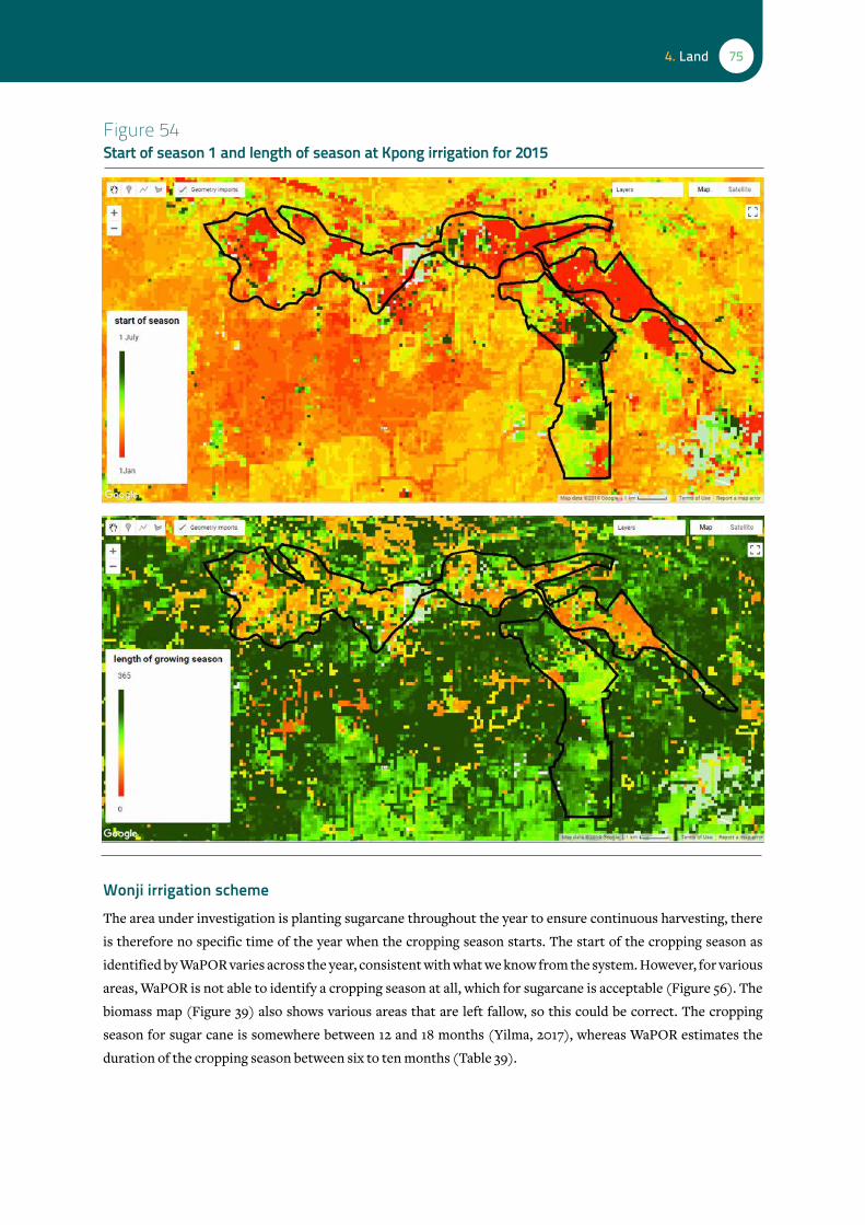
754. Land
Figure 54 Start of season 1 and length of season at Kpong irrigation for 2015
Wonji irrigation schemeThe area under investigation is planting sugarcane throughout the year to ensure continuous harvesting, there
is therefore no specific time of the year when the cropping season starts. The start of the cropping season as
identified by WaPOR varies across the year, consistent with what we know from the system. However, for various
areas, WaPOR is not able to identify a cropping season at all, which for sugarcane is acceptable (Figure 56). The
biomass map (Figure 39) also shows various areas that are left fallow, so this could be correct. The cropping
season for sugar cane is somewhere between 12 and 18 months (Yilma, 2017), whereas WaPOR estimates the
duration of the cropping season between six to ten months (Table 39).

76 WaPOR quality assessment
Table 37 Cropping season in Fayoum irrigation scheme
Crop Jan Feb Mar Apr May Jun Jul Aug Sep Oct Nov Dec
rice (s1)
rice (s2)
banana
legend: planting growing season harvesting
source: salvadore, 2019
Figure 55 Start of season 1 and length of season at Fayoum irrigation scheme for 2015
Table 38 WaPOR phenology indicators for Kpong irrigation scheme in 2015 (mean and standard deviation)
Start of s1 Duration of s1 Start of s2 Duration of s2
fayoum 10 October ± 7 months 73 ± 14 10 October ± 7 months 73 ± 14
Bekaa Valley irrigationThe irrigation in the Bekaa Valley, located in Lebanon follows the seasonality. An example of the cropping season
of a typical crop in the Bekaa Valley, potatoes, is provided in Table 40 (Alvarez-Carrion, 2018). Another wide
spread crop is wheat, which has for the winter varieties a cropping season of 100-170 days and for the summer
varieties 180-300 days. Because of the heterogeneity of the crop production in the Bekaa Valley it is difficult to
identify if the cropping season is well determined (Figure 57; Table 41).
start of season1 Jan
1 July
length of growing season365
0

774. Land
Figure 56 Start of season 1 and length of season at Kpong irrigation for 2015
Table 40 Cropping season of potatoes in Bekaa Valley irrigation
Crop Jan Feb Mar Apr May Jun Jul Aug Sep Oct Nov Dec
rice (s1)
rice (s2)
banana
legend: planting growing season harvesting
source: Alvarez-carrion, 2018
Table 39 WaPOR phenology indicators for Kpong irrigation scheme in 2015 (mean and standard deviation)
Start of s1 Duration of s1 Start of s2 Duration of s2
wonji 10 November ± 1 year 186 ± 61 20 April ± 10 months 104 ± 44
Consistency season 1 and season 2The WaPOR phenology produces separate layers for the start of season 1 and season 2. An analysis was done on
the start and end of all seasons identified by WaPOR for an area in Rwanda (Braliwa farms) (Figure 58). The area
is located in East Africa and experiences a bi-modal rainy season, with one season starting around October until
January and a second season from March to June. The season 1 (each red line in Figure 58 represents one pixel), in
2009 line up nicely. For 2010, some pixels span both the season November-January and March-June, other pixels
have the season October-January identified as season 2 for 2009 (green lines) and others have identified the same
season as season 1 for the year 2010. For the season October 2011-January 2012, the pixels are evenly identified as
2011 season 2 and 2012 season 1. For some pixels the same season is both identified as season 2 of a previous year
and season 1 of the following year (Annex E).
start of season1 July
1 Jan
length of growing season365
0

78 WaPOR quality assessment
Figure 57 Start of growing season 1 and length of growing season Bekaa Valley
Figure 58 Season 1 and season 2 pixel identification
Table 41 WaPOR phenology indicators for Bekaa Valley irrigation in 2015 (mean and standard deviation)
Start of season 1 Duration of season 1 Start of season 2 Duration of season 2
bekaa valley 20 Feb ± 6 months 162 ± 41 20 Feb ± 8 months 85 ± 24
bekaa_grapes 1 Feb ± 2 months 166 ± 47 20 March ± 8 months 101 ± 31
start of season1 July
1 Jan
length of growing season365
0

794. Land
C.3 ConclusionsThe WaPOR phenology layer generally presents the cropping season as expected at basin and national level,
following the general seasonality. However, when zooming into specific areas, the phenology layers has some
serious issues in adequately representing the cropping seasons. This is crucial for the WaPOR portal, as water
productivity is calculated on seasonal basis at Level 2, together with its inputs: seasonal AGBP and seasonally
cumulated AETI. If the season is not well defined, all other parameters are affected by this error. Also, the shift
between the two seasons, creates maps that are composed of pixels showing two different seasons. This makes
it difficult to analyse the data, also it hampers identifying trends between one year to the next (as it is not clear if
season 1 for year 1 is the same period as season 1 for year 2).
The main observation is that both crop types and cropping seasons cannot be obtained from WaPOR. Users have
to prepare their own crop masks and select the local cropping calendar. Only with this extra GIS processing, land
productivity, water productivity and crop water consumption can be properly estimated. It is recommended that
FAO and/or FRAME consortium will make this limitation and opportunity clear to website visitors.


Det
ail o
f WaP
OR
Map
“N
et B
iom
ass
Wat
er P
rodu
ctiv
ity
2014
- Ir
aq a
nd Ir
an”
5. Water productivity
A. Gross Water Productivity A.1 IntroductionThe WaPOR Water Productivity (WP) layers are based on a simple calculation of AGBP over AETI (gross biomass
WP or GBWP) and AGBP over T (net biomass WP or NBWP). The uncertainty of water productivity is therefore
directly related to the datasets of AGBP, AETI and T. The WaPOR data portal provides WP for integrated time
intervals. The 250 m resolution integrates WP on annual basis, whereas the 100 m and 30 m resolution data
integrates based on the WaPOR defined seasons.
A2. Data AnalysesThe WaPOR values for gross and net WP are presented in Figure 59. The average continental value of GBWP is 0.66
and for NBWP is 1.20. At first sight it is obvious that the arid zones exhibit lower WP values. This can be explained
by the fact that relative humidity and T are inversely related (low humidity will induce high T flux) while the C flux
is unaffected. The H20 and CO2 fluxes have to pass through the same stomatal aperture, and this climatological
control of WP by air humidity (thus also indirectly induced by air temperature) was recognized since the 1960s

82 WaPOR quality assessment
(Bierhuizen and Slayter, 1965). Indeed, the humid areas of Central Africa and the Atlas mountains in Morocco and
Algeria show the highest WP values, and these agro-ecosystems behave according to the theoretical expectations.
Some more attention should be provided to NBWP because biomass production per unit of transpiration is often
suggested to be conservative. It is also commonly referred to as the Transpiration Efficiency. Transpiration
Efficiency (TE) is a main feature in AquaCrop (Raes et al., 2011). The average value of 1.2 kg/m3 for NBWP for the
continent is on the low side, as the conservative relationship between biomass and transpiration for C3 crops
should be between 1.5 and 2.0 kg/m3 (Raes et al., 2011; Steduto et al., 2007).
Spatial data comparisonWe compared WaPOR gross WP with a similar product of Servir Mekong produced by Poortinga and co-workers
(Simons et al., 2017). The global WP map created by Servir uses the MODIS Terra NPP values and the SSEBop
AETI calculations and is therefore expressed in 0.1*kg C/m3 (Figure 60). We used the WaPOR NPP data and
WaPOR AETI to calculate WP in the same manner (converting to DM using the same conversion factors would
result in the same biases). The comparison shows large deviations between the two products, this can be both a
result of the differences in AETI or NPP. NPP differences between WaPOR and MOD17 (averaged for Terra and
Aqua though) were discussed in the earlier section on NPP, so we think the major difference originates from
AETI values estimated by SSEBop. Because WaPOR AETI was properly checked with water balances, it is believed
that WaPOR WP values are more accurate than the WP version created by Servir.
Figure 59 Average WaPOR gross biomass WP (GBWP) and net biomass WP (NBWP) for 2009-2017. Note that GBWP and NBWP are based on AGBP, thus ignore 35% of the total dry matter production
wapor net wp (kg/m3)
00.511.52
wapor gross wp (kg/m3)
00.511.52

835. Water productivity
Figure 60 Servir WP in 0.1*kg C/m3 and difference between Servir and WaPOR WP in 0.1*kg C/m3 (2009-2013)
Water productivity for selected irrigation scheme Gross and net Water Productivity (WP) was calculated for three of the four irrigation schemes. The Bekaa Valley
with the diverse cropping system was not included for the analyses. WP is defined as the yield per unit of water
(kg/m3), the gross WP uses the total water consumption (AETI), whereas the net WP uses T for unit of water
beneficially consumed.
Wonji irrigation schemeThe gross WP for sugar cane in the Wonji irrigation scheme, was calculated using the 30 m resolution data (Figure
61). Gross WP is 5.22 kg/m3 (Table 42), which is on the low side compared to the range of 5.9-6.6 kg/m3 found by
Yilma (2017). The values found by Yilma were individual plot values, whereas the WaPOR data is an integrated
value of the entire area, including fallow plots and buildings and areas with open water, thereby lowering the
average value for gross WP. The WaPOR estimated value for gross WP is therefore in the correct range.
servir gross wp (0.1*kgc/m3)
00.511.52
servir wapor gross wp (0.1*kgc/m3)
-2-1012

84 WaPOR quality assessment
Figure 61 Gross WP for Wonji (30 m resolution)
Table 42 Key indicators for Water Productivity in Wonji irrigation scheme
Yield (tonnes/ha) AETI (mm/season) T (mm/season) Gross WP (kg/m3) Net WP (kg/m3)
sugarcane 99.85 1,926 1,638 5.22 6.13
Fayoum irrigation schemeThe gross and net WP for the Fayoum irrigation scheme are presented in Figure 62 and Table 43. Salvadore (2019)
found for wheat gross WP of 0.94, for maize 0.75 and for oranges 1.55 kg/m3. The values found using WaPOR
data are slightly higher. The areas presumed to be fallow (low biomass production, see also Figure 48) around
the edges of the irrigation scheme show the highest gross WP. This indicates that WP on its own is not a good
indicator for agricultural productivity. Considering these differences, the WaPOR gross WP values provide a
good reference for WP calculations.

855. Water productivity
Figure 62 Gross Water Productivity wheat and maize
Table 43 Key indicators for Water Productivity in Wonji irrigation scheme
Yield (tonnes/ha) AETI (mm/season) T (mm/season) Gross WP (kg/m3) Net WP (kg/m3)
wheat 5.28 248 178 1.11 1.25
maize 3.14 244 159 0.69 0.87
oranges 24.69 485 333 1.83 2.02
Kpong irrigation schemeThe gross WP for Kpong irrigation scheme is presented in Figure 63 and 64 and Table 44. The gross WP for rice
1.18 and for banana it is 4.85 kg/m3. We did not have locally verified values to compare the gross WP with. However,
what is clear is that in humid climate, the differentiation between agricultural land and natural vegetation is not
clear. For rice during both seasons, the surrounding landscape seems to have higher WP compared to the irrigated
system. Without a detailed land use map it is not possible to correctly estimate agricultural water productivity, as
natural vegetation would be erroneously included in the biomass production estimations.
wp (kg/m3)
2
0
wp (kg/m3)
2
0

86 WaPOR quality assessment
Figure 63 Kpong gross WP rice season 1 (top) and season 2 (bottom)
Table 44 Kpong gross WP rice season 1 (top) and season 2 (bottom)
Yield (tonnes/ha) AETI (mm/season) T (mm/season) Gross WP (kg/m3) Net WP (kg/m3)
banana 37.59 1,022 793 3.72 4.85
rice s1 4.15 495 356 0.86 1.25
rice s2 3.99 503 382 0.82 1.11
wp (kg/m3)
2
0
wp (kg/m3)
2
0

875. Water productivity
Figure 64 Kpong gross WP bananas
C3. ConclusionsThe WaPOR gross WP using user defined cropping season, harvest index and moisture content values, provides
very good estimation of WP. The gross WP estimates for sugarcane (Ethiopia) and wheat (Egypt) highlight the
challenges of deriving such indicators from remote sensing. In the Ethiopia case, the areal gross WP is lower than
the field observation as the area incorporates non-agricultural or fallow land in the analyses. For Egypt, fallow
land increases the areal gross WP, as fallow areas (with low AGBP and even lower AETI) reflect with a high WP.
The inaccuracy of WP in those cases seems to originate from wrong identification of cultivated areas and not
from erroneous WP assessment.
For the humid area in Ghana, the main challenges is the differentiation of natural vegetation versus agricultural
lands. The surrounding landscape has equal or higher WP compared to the irrigated areas. It is expected that
rainfed agricultural areas will face similar challenges in distinguishing between natural and agricultural lands, as
both follow similar phenological patterns.


Det
ail o
f WaP
OR
Map
“P
heno
logy
Sea
son
end
2010
- C
entr
al A
fric
an R
epub
lic, S
udan
, Sou
th S
udan
and
Eth
iopi
a”
6. SynthesisRainfall in WaPOR is based on the spatial CHIRPS rainfall product. This is an existing product that is widely tested in
the international literature. Research in Africa and Asia supports the selection of this product. Not only the quality
is good, the spatial resolution of 5 km x 5 km is superior as well and the data goes back as far as 1983, which makes it
suitable for climate change studies and impact on crop production. For a proper independent validation of CHIRPS,
it is required to have access to a network with a high density of rainfall gauges. There is currently a spatial mismatch
between the coverage of CHIRPS and that of rain gauges. Therefore areas with a higher density of rain gauges need
to be searched for further validation of the CHIRPS product. Due to the fact that CHIRPS is an existing product, we
have deliberately chosen to focus for now on the validation of the AETI and biomass production products.
Obviously, WaPOR follows the FAO standard guidelines on reference evapotranspiration as laid out in FAO
Irrigation and Drainage paper 56. Because the methodology is a global standard, the quality control should focus
on the inputs for the FAO 56 equation. While WaPOR makes use of MERRA, it seems there are also advantages of
using GLDAS. More routine weather stations should be involved in the next phase of the validation analysis to verify
whether MERRA or GLDAS is more accurate. For now, it is convenient to conclude that no suspicious results of RET
were found.

90 WaPOR quality assessment
While AETI cannot be measured in a straightforward manner, most of the in situ techniques available for an
independent ground truth have been explored. These techniques range from eddy covariance flux towers, soil water
balances at field scale to river basin water balances. Field measurements from many different countries in North
Africa, Near East and Eastern Africa could be included in the analysis. While this would take more time, it helps in
drawing consistent conclusions.
The overall finding is that the accumulated AETI for a year is rather good, and that spatially aggregated AETI
values for river basins or sub-basins (e.g. 11 sub-basins of the Nile system) match even better. Some error in the
accumulated and spatially aggregated AETI of WaPOR seems to be introduced at higher aridity. For instance, the
Nile Delta, Fayoum Depression and Jordan River show higher deviation. Various mismatches with local fields and
for shorter periods were detected. During the period of full crop development, AETI hardly exceeds 5 mm/d. The
latter is essential for FAO, as a significant part of the applications will be related to crop water productivity analysis
for a shorter period and for particular fields.
The breakdown of AETI into T, E and I has emphasized that T/AETI is higher than comparative remote sensing
models and international literature. While we believe that T/AETI is at the higher side indeed, for instance the
Transpiration Efficiencies (or NBWP in WaPOR terms) seem too low, T should increase during peak growing
season and decrease in the emergence, senescence and fallow period. The interactions between LAI, PCP, soil
moisture and light extinction coefficient α need to be investigated with more attention.
The biomass production and the related NPP fluxes are rather good for pristine growing conditions. The crop yield
for various crops can now be computed in a physical manner, provided that the proper conversion factors are used.
This is a leap forward as compared to solutions based on empirical relationships with NDVI. With WaPOR a decent
bio-physical methodology is available with consistent data across a period of ten years.
The WP is based on biomass production, and not on crop yield. GBWP is a surrogate for WP by absence of crop
information. The default constants of root-shoot ratio and maximum light use efficiency are questionable, and
require more time for validation. It is easier to compare WP for yield for which more international literature is
available, however this requires local knowledge to convert AGBP or TBP to yield.
Problematic are the layers on rainfed and irrigated crops, along with their cropping calendar. These two parameter
are related because cropland has specific days of emergence and harvest and confusion between cropland and
other land use will immediately impact the detection of the duration of the cropping and irrigation seasons. With
user knowledge on the location of the field, crop type and cropping season, the WaPOR database is able to derive
acceptable results.

Det
ail o
f WaP
OR
Map
“A
nnua
l Tra
nspi
rati
on 2
009
- Dem
ocra
tic
Rep
ublic
of t
he C
ongo
, Rep
ublic
of t
he C
ongo
and
Gab
on”
7. Next stepsA disturbing role of aridity on the accuracy of AETI values for different products has been found, with WaPOR
performing better than other products, but still with some bias. The causing factors for this sensitivity need to be
found out as a collaborative effort with the WaPOR team. Not unlikely, the combined soil moisture, temperature
and vapor pressure deficit stress plays a regulating role on the stomatal behavior that requires correction.
The estimates of T in WaPOR is inspected and evaluated. While local sapflow measurements showed the opposite,
we believe that T is genuinely high. The breakdown of T in smaller periods needs to be investigated. Additional
analysis with basal crop coefficients using NDVI are required for assessing the potential transpiration rates.
Furthermore, T data layers should be compared with AGBP and TBP values for specific land use and crop types.
The WP parameter introduced in AquaCrop is normalized for atmospheric evaporative demand, defined by ET0,
and for the CO2 concentration of the atmosphere. The normalized biomass water productivity (WP*) proved to
be nearly constant for a given crop when mineral nutrients are not limiting, regardless of water stress except for
extremely severe cases. Normalization NBWP for evaporative demands and atmospheric CO2 concentration has to
be executed and the conservation behavior of the normalized AGBP should be verified.

92 WaPOR quality assessment
More sources of land cover and land use need to be consulted to improve the WaPOR LCC. High resolution data
bases became available recently such as the CCI land cover at 20 m spatial resolution from the Joint Research
Centre JRC (http://2016africalandcover20m.esrin.esa.int/), GeoWiki from IIASA (https://www.geo-wiki.org/),
the Global Food Security-Support Analysis Data at 30 m from USGS (https://www.usgs.gov/centers/wgsc/science/
global-food-security-support-analysis-data-30-m?qt-science_center_objects=0#qt-science_center_objects) and
the global land cover map of Tsinghua University (http://data.ess.tsinghua.edu.cn/). Together with new solutions to
detect irrigation processes, this could be considered to improve the current WaPOR maps on rainfed and irrigated
cropland.

93References
ReferencesAbatzoglou, J. T., Dobrowski, S. Z., Parks, S. A., & Hegewisch, K. C. 2018. TerraClimate, a high-resolution global
dataset of monthly climate and climatic water balance from 1958–2015. Scientific data, 5, 170191.
Alemohammad, S. H., Fang, B., Konings, A. G., Aires, F., Green, J. K., Kolassa, J., Miralles, D., Prigent, C., &
Gentine, P. 2017. Water, Energy, and Carbon with Artificial Neural Networks (WECANN): a statistically based
estimate of global surface turbulent fluxes and gross primary productivity using solar-induced fluorescence.
Biogeosciences, 14(18), 4101-4124.
Allen, R. G., Pereira, L. S., Raes, D., & Smith, M. 1998. Crop evapotranspiration-Guidelines for computing crop
water requirements-FAO Irrigation and drainage paper 56. Fao, Rome, 300(9), D05109.
Allen, R. G., Pereira, L. S., Smith, M., Raes, D., & Wright, J. L. 2005. FAO-56 dual crop coefficient method for
estimating evaporation from soil and application extensions. Journal of irrigation and drainage engineering,
131(1), 2-13.
Alvarez-Carrion, S.M. 2018. Water Productivity score computation using spatial remote sensing data sources in
the Bekaa valley, Lebanon. UNESCO-IHE MSc thesis. 70 pages
Anderson, M. C., Norman, J. M., Mecikalski, J. R., Otkin, J. A., & Kustas, W. P. 2007. A climatological study of
evapotranspiration and moisture stress across the continental United States based on thermal remote sensing:
1. Model formulation. Journal of Geophysical Research: Atmospheres, 112(D10).
Archibald, S. A., Kirton, A., Merwe, M. R. van der, Scholes, R. J., Williams, C. A. and Hanan, N. 2009. Drivers
of inter-annual variability in Net Ecosystem Exchange in a semi-arid savanna ecosystem, South Africa,
Biogeosciences, 6(2), 251–266.
Arnold, J.G., Bieger, K., White, M.J., Srinivasan, R., Dunbar, J.A., Allen, P.M. 2018. Use of decision tables to
simulate management in SWAT+. Water (Switzerland) 10, 1–10. https://doi.org/10.3390/w10060713
Arnold, J.G., Srinivasan, R., Muttiah, R.S., Williams, J.R. 1998. LARGE AREA HYDROLOGIC MODELING AND
ASSESSMENT PART I: MODEL DEVELOPMENT. J. Am. Resour. Assoc. 34, 73–89. https://doi.org/10.1016/
S0899-9007(00)00483-4
Awange, J. L., Ferreira, V. G., Forootan, E., Andam-Akorful, S. A., Agutu, N. O., & He, X. F. 2016. Uncertainties in
remotely sensed precipitation data over Africa. International Journal of Climatology, 36(1), 303-323.
Baldocchi, D. D., Hincks, B. B., and Meyers, T. P.: Measuring Biosphere-Atmosphere Exchanges of Biologically
Related Gases with Micrometeorological Methods, Ecology, 69, 1331– 1340, 1988.
93

94 WaPOR quality assessment
Bastiaanssen, W. G. M., Cheema, M. J. M., Immerzeel, W. W., Miltenburg, I. J., & Pelgrum, H. 2012. Surface
energy balance and actual evapotranspiration of the transboundary Indus Basin estimated from satellite
measurements and the ETLook model. Water Resources Research, 48(11).
Bastiaanssen, W.G.M., Karimi, P., Rebelo, L.M., Duan, Z., Senay, G., Muthuwatte, L., Smakhtin, V. 2014. Earth
observation based assessment of the water production and water consumption of Nile basin agro-ecosystems.
Remote Sens. 6, 10306–10334. https://doi.org/10.3390/rs61110306
Bastidas-Obando, E., Bastiaanssen, W.G.M., Jarmain, C. 2017. Estimation of transpiration fluxes from rainfed
and irrigated sugarcane in South Africa using a canopy resistance and crop coefficient model. Agric. Water
Manag. 181, 94–107. https://doi.org/10.1016/j.agwat.2016.11.024
Belete, M., Deng, J., Zhou, M., Wang, K., You, S., Hong, Y., Weston, M. 2018. A new approach to modelingwater
balance in Nile River Basin, Africa. Sustain. 10, 1–14. https://doi.org/10.3390/su10030810
Bieger, K., Arnold, J.G., Rathjens, H., White, M.J., Bosch, D.D., Allen, P.M., Volk, M., Srinivasan, R. 2017.
Introduction to SWAT+, a Completely Restructured Version of the Soil and Water Assessment Tool. J. Am.
Water Resour. Assoc. 53, 115–130. https://doi.org/10.1111/1752-1688.12482
Bierhuizen, J.F., and R.O. Slayter. 1965. Effect of atmospheric concentration of water vapor and CO2 in determining
transpiration-photosynthesis relationships of cotton leaves. Agric. Meteorol. 2:259–270.
Bouchet, R. J., 1963. Evapotranspiration réelle evapotranspiration potentielle, signification climatique, pp. 134–
142, in International Association of Scientific Hydrology, General Assembly of Berkeley, Transactions, vol. 2,
Evaporation, Berkeley, California.
Calera, A., Martínez, C., Meliá, J. 2001. A procedure for Obtaining Green Plant Cover: Relation to NDVI in a Case
of Study for Barley. International Journal of Remote Sensing, vol 22, no 17, 3357-3362.
Cheema, M.J.M. and W.G.M. Bastiaanssen 2012. Local calibration of remotely sensed rainfall from the TRMM
satellite for different periods and spatial scales in the Indus Basin, Int. J. Of Rem. Sens., 33(8): 2603-2627
Chen, Y., Lu, D., Luo, L., Pokhrel, Y., Deb, K., Huang, J., & Ran, Y. 2018. Detecting irrigation extent, frequency, and
timing in a heterogeneous arid agricultural region using MODIS time series, Landsat imagery, and ancillary data.
Remote Sensing of Environment, 204, 197-211.
Chiti, T., Certini, G., Grieco, E. and Valentini, R. 2010. The role of soil in storing carbon in tropical rainforests: the
case of Ankasa Park, Ghana, Plant Soil, 331, 453-461.
Choudhury, B. J., & DiGirolamo, N. E. 1998. A biophysical process-based estimate of global land surface
evaporation using satellite and ancillary data I. Model description and comparison with observations. Journal
of Hydrology, 205(3-4), 164-185.

95References
Conway, G. 2009. The science of climate change in Africa: impacts and adaptation. Grantham Institute for
Climate Change Discussion Paper, 1, 24.
De Bruin, H. A. R., Trigo, I. F., Bosveld, F. C., & Meirink, J. F. 2016. A thermodynamically based model for actual
evapotranspiration of an extensive grass field close to FAO Reference, suitable for remote sensing application.
Journal of Hydrometeorology, 17(5), 1373-1382.
Dee, D. P., Uppala, S. M., Simmons, A. J., Berrisford, P., Poli, P., Kobayashi, S., Andrae, U., Balmaseda, M.A.,
Balsamo, G., Bauer, P., Bechtold, P., Beljaars, A.C.M., van de Berg, L., Bidlot, J., Bormann, N., Delsol, C.,
Dragani, R., Fuentes, M., Geer, A.J., Haimberger, L., Healy, S.B., Hersbach, H., Hólm, E.V., Isaksen, L.,
Kållberg, P., Köhler, M., Matricardi, M., McNally, A.P., Monge-Sanz, B.M., Morcrette, J.-J., Park, B.-K.,
Peubey, C., de Rosnay, P., Tavolato, C., Thépaut, J.-N., & Vitart, F. 2011. The ERA-Interim reanalysis:
Configuration and performance of the data assimilation system. Quarterly Journal of the royal meteorological
society, 137(656), 553-597.
Dembélé, M., & Zwart, S. J. 2016. Evaluation and comparison of satellite-based rainfall products in Burkina Faso,
West Africa. International journal of remote sensing, 37(17), 3995-4014.
Dheeravath, V., Thenkabail, P.S., Chandrakantha, G., Noojipady, P., Reddy, G.P.O., Biradar, C.M., Gumma,
M.K., Velpuri, M. 2010. Irrigated areas of India derived using MODIS 500 m time series for the years 2001 - 2003.
ISPRS Journal of Photogrammetry and Remote Sensing, 65 (1), 42-59.
Dinku, T., Funk, C., Peterson, P., Maidment, R., Tadesse, T., Gadain, H., & Ceccato, P. 2018. Validation of the
CHIRPS satellite rainfall estimates over eastern of Africa. Quarterly Journal of the Royal Meteorological Society.
Dobrowski, S. Z., Abatzoglou, J., Swanson, A. K., Greenberg, J. A., Mynsberge, A. R., Holden, Z. A., & Schwartz,
M. K. 2013. The climate velocity of the contiguous United States during the 20th century. Global change biology,
19(1), 241-251.
El-Quosy, Dia and Samia El-Guindy. 1989. Water and salt balance of the Nile Delta, a new approach, in (eds.) M.H
Amer and N.A. de Ridder, Land Drainage in Egypt, Chapter 10: 243-253
FAO. 2016. AQUASTAT website. Food and Agriculture Organization of the United Nations (FAO). Website
accessed on 2018/12/27.
FAO. 2018. WaPOR Database Methodology: Level 1. Remote Sensing for Water Productivity Technical Report:
Methodology Series. Rome, FAO. 72 pages. http://www.fao.org/3/I7315EN/i7315en.pdf
FAO. 2019. El Nino and rainfall. http://www.fao.org/emergencies/resources/maps/detail/en/c/339920/ Accessed on
19-01-2019

96 WaPOR quality assessment
Fisher, J.B., Melton, F., Middleton, E., Hain, C., Anderson, M., Allen, R., Mccabe, M.F., Hook, S., Baldocchi, D.,
Townsend, P.A., Kilic, A., Tu, K., Miralles, D.D., Perret, J., Lagouarde, J.-P., Waliser, D., Purdy, A.J., French,
A., Schimel, D., Famiglietti, J.S., Stephens, G., Wood, E.F. 2017. The future of evapotranspiration: Global
requirements for ecosystem functioning, carbon and climate feedbacks, agricultural management, and water
resources. Water Resour. Res. 53, 2618–2626. https://doi.org/10.1002/2016WR020175
Foley, J.A., C.J. Kucharik, and D. Polzin. 2005. Integrated Biosphere Simulator Model (IBIS), Version 2.5. ORNL
DAAC, Oak Ridge, Tennessee, USA. https://doi.org/10.3334/ORNLDAAC/808
Funk, C., Peterson, P., Landsfeld, M., Pedreros, D., Verdin, J., Shukla, S., Husak, G., Rowland, J., Harrison, L.,
Hoell, A., Michaelsen, J. 2015. The climate hazards infrared precipitation with stations—a new environmental
record for monitoring extremes. Scientific data, 2, 150066.
Ghana Irrigation Development Authority (GIDA). 2010. Feasibility of the Accra Plains Irrigation Project –
Detailed study for the 5000 ha. Final report, 300 pages
Gilmont, M., Al Naber, M., Tal, N., and Alhaddadin, R. 2019. Water Productivity Decoupling – Verification of
agricultural potential for Jordan and Israel using farm-level surveys and remote sensing in Jordan Valley. Draft
Project Report
Gilmont, M., Nassar, L., Rayner, S., Tal, N., Harper, E., Salem, H.S. 2018. The Potential for Enhanced Water
Decoupling in the Jordan Basin through Regional Agricultural Best Practice, Land, 7, 63; doi:10.3390/land7020063
Guerschman, J.P., Van Dijk, A.I., Mattersdorf, G., Beringer, J., Hutley, L.B., Leuning, R., Pipunic, R.C., &
Sherman, B.S. 2009. Scaling of potential evapotranspiration with MODIS data reproduces flux observations
and catchment water balance observations across Australia. Journal of Hydrology, 369(1-2), 107-119.
Ha, L.T., W.G.M. Bastiaanssen, A. van Griensven, A.I.J.M. van Dijk, and G.l B. Senay. 2017. SWAT-CUP for
Calibration of Spatially Distributed Hydrological Processes and Ecosystem Services in a Vietnamese River Basin
Using Remote Sensing, https://doi.org/10.5194/hess-2017-251
Hargreaves, G.H., and Z.A. Samani. 1985. Reference crop evapotranspiration from temperature. Applied
Engineering. in Agric. 1:96-99
Harris, I.C.; Jones, P.D. 2017. CRU TS4.00: Climatic Research Unit (CRU) Time-Series (TS) version 4.00 of
high-resolution gridded data of month-by-month variation in climate (Jan. 1901- Dec. 2015). Centre for
Environmental Data Analysis, 25 August 2017. doi:10.5285/edf8febfdaad48abb2cbaf7d7e846a86
HarvestChoice. 2011. "Longterm Average Annual Rainfall (mm)." International Food Policy Research Institute,
Washington, DC., and University of Minnesota, St. Paul, MN. Available online at http://harvestchoice.org/
node/4963.

97References
Heinsch, F. A., Reeves, M., Votava, P., Kang, S., Milesi, C., Zhao, M., Glassy, J., Jolly, W.M., Loehman, R., Bowker,
C.F., Kimball, J.S., Nemani, R.R., & Running, S.W. 2003. GPP and NPP (MOD17A2/A3) Products NASA MODIS
Land Algorithm. MOD17 User's Guide, 1-57.
Herman, A., V. B. Kumar, P. A. Arkin, and J. V. Kousky. 1997. “Objectively Determined 10-Day African Rainfall
Estimates Created for Famine Early Warning Systems.” International Journal of Remote Sensing 18 (10): 2147–
2159. doi:10.1080/014311697217800
Hessels, T. M. 2015. Comparison and Validation of Several Open Access Remotely Sensed Rainfall Products for the
Nile Basin. MSc thesis TU Delft
Hilhorst, B.; Burke, J.; Hoogeveen, J.; Fremken, K.; Faures, J.-M.; Gross, D. 2011. Information Products for Nile
Basin Water Resources Management; FAO: Rome, Italy; p. 130
Hsu, K.-L., X. Gao, S., Sorooshian, and Gupta, H.V. 1997. “Precipitation Estimation from Remotely Sensed
Information Using Artificial Neural Networks.” Journal of Applied Meteorology 36 (9): 1176–1190.
doi:10.1175/1520-0450(1997)0362.0.CO;2.
Hu, G., & Jia, L. 2015. Monitoring of evapotranspiration in a semi-arid inland river basin by combining microwave
and optical remote sensing observations. Remote Sensing, 7(3), 3056-3087.
Jiménez, C., Prigent, C., Mueller, B., Seneviratne, S.I., McCabe, M.F., Wood, E.F., Rossow, W.B., Balsamo, G.,
Betts, A.K., Dirmeyer, P.A., Fisher, J.B., Jung, M., Kanamitsu, M., Reichle, R.H., Reichstein, M., Rodell, M.,
Sheffield, J., Tu, K., Wang, K. 2011. Global intercomparison of 12 land surface heat flux estimates. J. Geophys.
Res. Atmos. 116, 1–27. https://doi.org/10.1029/2010JD014545
Joyce, R.J., Janowiak, J.E., Arkin, P.A., Xie, P. 2004. CMORPH: a method that produces global precipitation
estimates from passive microwave and infrared data at high spatial and temporal resolution. J. Hydrometeorol.
5 : 487–503
Jung, M., Reichstein, M., Ciais, P., Seneviratne, S. I., Sheffield, J., Bonan, G., Chen, J., Cescatti, A., de Jeu, R.A.M.,
Dolman, A. J., Eugster, W., Gerten, D., Gianelle, D., Gobron, N., Goulden, M. L., Heinke, J., Kimball, J., Law,
B.E., Montagnani, J., Mu, Q., Mueller, B., Oleson, K., Papale, D., Richardson, A., Roupsard, O., Running, S.,
Tomelleri, E., Viovy, N., Weber, U., Williams, C., Wood, E., Zaehle, S., & Zhang, K. 2010. Recent decline in the
global land evapotranspiration trend due to limited moisture supply. Nature 467:951– 954
Jung, H.C., Getirana, A., Policelli, F., McNally, A., Arsenault, K.R., Kumar, S., Tadesse, T., Peters-Lidard, C.D.
2017. Upper Blue Nile basin water budget from a multi-model perspective. J. Hydrol. 555, 535–546. https://doi.
org/10.1016/j.jhydrol.2017.10.040
Jung, M., Reichstein, M. & Bondeau, A. 2009. Towards global empirical upscaling of FLUXNET eddy covariance
observations: validation of a model tree ensemble approach using a biosphere model. Biogeosciences 6, 2001–
2013.

98 WaPOR quality assessment
Karimi, P., Molden, D., Notenbaert, A., Peden, D. 2012. Nile basin farming systems and productivity. In The Nile
River Basin, Water, Agriculture, Governance and Livelihoods; Chalmers, K., Godfrey, J., Eds.; Edgar Elger:
Cheltenham, UK, 2012; pp. 133–153
Kiptala, J.K., Mohamed, Y., Mul, M.L., Zaag, P. 2013. Mapping evapotranspiration trends using MODIS and SEBAL
model in a data scarce and heterogeneous landscape in Eastern Africa. Water Resour. Res. 49, 8495–8510.
Kongo, M.V., Jewitt, G.W.P., & Lorentz, S.A. 2011. Evaporative water use of different land uses in the upper-
Thukela river basin assessed from satellite imagery. Agricultural water management, 98(11), 1727-1739.
Kucharik, C.J., Foley, J.A., Delire, C., Fisher, V.A., Coe, M.T., Lenters, J.D., Young-Molling, C., Ramankutty,
N., Norman, J.M., & Gower, S.T. 2000. Testing the performance of a dynamic global ecosystem model: water
balance, carbon balance, and vegetation structure. Global Biogeochemical Cycles, 14(3), 795-825.
Łabędzki, L. 2011. Evapotranspiration Edited. InTech, Rijeka, Croatia.
Li, A., Bian, J., Lei, G., & Huang, C. 2012. Estimating the maximal light use efficiency for different vegetation
through the CASA Model combined with time-series remote sensing data and ground measurements. Remote
sensing, 4(12), 3857-3876.
Madani, N., Kimball, J.S., & Running, S.W. 2017. Improving global gross primary productivity estimates by
computing optimum light use efficiencies using flux tower data. Journal of Geophysical Research: Biogeosciences,
122(11), 2939-2951.
Maidment, R.I., D. Grimes, R.P. Allan, E. Tarnavsky, M. Stringer, T. Hewison, R. Roebeling, and E. Black.
2014. “The 30 Year TAMSAT African Rainfall Climatology and Time Series (TARCAT) Data Set.” Journal of
Geophysical Research: Atmospheres 119 (18): 10,619–610,644. doi:10.1002/ 2014JD021927
Marchesini, B., L., Bombelli, A., Chiti, T., Consalvo, C., Forgione, A., Grieco, E., Mazzenga, F., Papale, D.,
Stefani, P., Vittorini, E., Zompanti, R., & Valentini, R. 2011. Ankasa flux tower: a new research facility for the
study of the carbon cycle in a primary tropical forest in Africa. Africa and the Carbon Cycle, 11.
Marshall, M., Tu, K., Funk, C., Michaelsen, J., Williams, P., Williams, C., Ardö, J., Boucher, M., Cappelaere, B.,
De Grandcourt, A., Nickless A., Nouvellon, Y., Scholes, R., & Kutsch, W. 2013. Improving operational land
surface model canopy evapotranspiration in Africa using a direct remote sensing approach. Hydrology and
Earth System Sciences 17, 1079–1091
Martens, B., Miralles, D.G., Lievens, H., Van Der Schalie, R., De Jeu, R.A.M., Fernández36 Prieto, D., Beck, H.E.,
Dorigo, W.A., Verhoest, N.E.C. 2017. GLEAM v3 : satellite-based land evaporation and root-zone soil moisture.
Geosci. Model Dev. 10, 1903–1925, doi:10.5194/gmd-10-1903-2017.

99References
Mianabadi, A., Coenders–Gerrits, M., Shirazi, P., Ghahraman, B., & Alizadeh, A. 2019. A global Budyko model to
partition evaporation into interception and transpiration. Hydrology and Earth System Sciences Discussions
https://doi.org/10.5194/hess-2018-638, in review.
Michel, D., Jiménez, C., Miralles, D.G., Jung, M., Hirschi, M., Ershadi, A., Martens, B., McCabe, M.F., Fischer,
J.B., Mu, Q., Seneviratne, S.I., Wood, E.F., & Fernàndez-Prieto, D. 2016. TheWACMOS-ET project–Part 1:
Tower-scale evaluation of four remote-sensing-based evapotranspiration algorithms. Hydrology and Earth
System Sciences, 20(2), 803-822.
Miralles, D.G., De Jeu, R.A.M., Gash, J.H., Holmes, T.R.H., and Dolman, A.J. 2011a. Magnitude and variability of
land evaporation and its components at the global scale, Hydrol. Earth Syst. Sci., 15, 967–981, doi:10.5194/hess-
15-967-2011.
Miralles, D.G., Holmes, T.R.H., De Jeu, R.A.M., Gash, J.H., Meesters, A.G.C.A., and Dolman, A.J. 2011b. Global
land-surface evaporation estimated from satellite-based observations, Hydrol. Earth Syst. Sci., 15, 453–469,
doi:10.5194/hess-15-453-2011
Miralles, D.G., Jiménez, C., Jung, M., Michel, D., Ershadi, A., Mccabe, M.F., Hirschi, M., Martens, B., Dolman,
A.J., Fisher, J.B., Mu, Q., Seneviratne, S.I., Wood, E.F., Fernández-Prieto, D. 2016. The WACMOS-ET project-
Part 2: Evaluation of global terrestrial evaporation data sets. Hydrol. Earth Syst. Sci 20, 823–842. https://doi.
org/10.5194/hess-20-823-2016
Monteith, J.L. 1965. Evaporation and environment. 19th Symposia of the Society for Experimental Biology 19: 205-
234.
Mu, Q., F. A. Heinsch, M. Zhao, and S. W. Running. 2007. Development of a global evapotranspiration algorithm
based on MODIS and global meteorology data, Remote Sens. Environ., 111, 519–536.
Mu, Q., Heinsch, F.A., Zhao, M., Running, S.W. 2011. Development of a global evapotranspiration algorithm based
on MODIS and global meteorology data. Remote Sensing of Environment 111, 519–536. https://doi.org/10.1016/j.
rse.2007.04.015
Mu, Q., M. Zhao, and S. W. Running. 2011. Improvements to a MODIS global terrestrial evapotranspiration
algorithm, Remote Sens. Environ., 115, 1781–1800.
Mueller, B., Hirschi, M., Jimenez, C., Ciais, P., Dirmeyer, P. A., Dolman, A. J., Fisher, J. B., Jung, M., Ludwig, F.,
Maignan, F., Miralles, D. G., McCabe, M. F., Reichstein, M., Sheffield, J., Wang, K., Wood, E. F., Zhang, Y.,
and Seneviratne, S. I. 2013. Benchmark products for land evapotranspiration: LandFluxEVAL multi-data set
synthesis, Hydrol. Earth Syst. Sci., 17, 3707–3720, doi:10.5194/hess-17-3707-2013, 2013.
New, M., Lister, D., Hulme, M., Makin, I. 2000. A high-resolution data set of surface climate over global land areas.
Climate Research, Vol 21: 1-25, http://dx.doi.org/10.3354/cr021001
100 WaPOR quality assessment
Nile Basin Initiative. 2014. Mapping Actual Evapotranspiration over the Nile Basin.
Novella, N., and W. Thiaw. 2010. Validation of Satellite-Derived Rainfall Products over the Sahel, 1–9. Camp
Springs, MD: Wyle Information Systems/CPC/NOAA.
Novella, N. S., and W. M. Thiaw. 2013. “African Rainfall Climatology Version 2 for Famine Early Warning Systems.”
Journal of Applied Meteorology and Climatology 52 (3): 588–606. doi:10.1175/ JAMC-D-11-0238.1
Paca, V. H. da Motta, G. E. Espinoza-Dávalos, T.M. Hessels, D. Medeiros Moreira, G.F. Comair and W.G.M.
Bastiaanssen. 2019. The spatial variability of actual evapotranspiration across the Amazon River Basin based
on remote sensing products validated with flux towers, Ecological Processes, Springer, https://doi.org/10.1186/
s13717-019-0158-8
Penman, H.L. 1963. Vegetation and hydrology. Technical Communication No. 53. Harpenden, England:
Commonwealth Bureau of Soils. 125p.
Pôças, I., Paço, T. A., Paredes, P., Cunha, M., & Pereira, L. S. 2015. Estimation of actual crop coefficients using
remotely sensed vegetation indices and soil water balance modelled data. Remote Sensing, 7(3), 2373-2400.
Poméon, T., Jackisch, D., & Diekkrüger, B. 2017. Evaluating the performance of remotely sensed and reanalysed
precipitation data over West Africa using HBV light. Journal of hydrology, 547, 222-235.
Poortinga et al. (in prep. a). Water accounting for the Awash river basin
Poortinga et al. (in prep. b). Water accounting for the Jordan and Litani river basins
Raes, D., Steduto, P., Hsiao, T.C. & Fereres, E. 2011. Aquacrop – Reference Manual. Available at: http://www.fao.
org/nr/water/aquacrop.html
Ramadan, F.M, D.S. Alnaggar and H.M van Leeuwen. 1989. The Fayoum water and salt balance model, in (eds)
M.H Amer and N.A. de Ridder, Land Drainage in Egypt, chapter 11: 255-294
Richard, Y., S. Trzaska, P. Roucou, and M. Rouault. 2000. Modification of the southern African rainfall variability/
ENSO relationship since the late 1960s. Climate Dyn., 16, 883–895, doi:10.1007/s003820000086.
Rockström, J. 2003. Water for food and nature in drought–prone tropics: vapour shift in rain–fed agriculture.
Philosophical Transactions of the Royal Society of London B: Biological Sciences, 358(1440), 1997-2009.
Rodell, M., P.R. Houser, U. Jambor, J. Gottschalck, K. Mitchell, C.-J. Meng, K. Arsenault, B. Cosgrove, J.
Radakovich, M. Bosilovich, J.K. Entin, J.P. Walker, D. Lohmann, and D. Toll. 2004. The Global Land Data
Assimilation System, Bull. Amer. Meteor. Soc., 85(3), 381-394.
Ruimy, A., Kergoat, L., & Bondeau, A. 1999. Comparing global models of terrestrial net primary productivity
(NPP): Analysis of differences in light absorption and light-use efficiency. Global Change Biology, 5(S1), 56-64.

101References
Running, S. W., & Zhao, M. 2015. Daily GPP and annual NPP (MOD17A2/A3) products NASA Earth Observing
System MODIS land algorithm. MOD17 User’s Guide.
Running, S., Mu, Q., Zhao, M. 2015. MOD17A3H MODIS/Terra Net Primary Production Yearly L4 Global 500m SIN
Grid V006 [Data set]. NASA EOSDIS Land Processes DAAC. doi: 10.5067/MODIS/MOD17A3H.006
Saah, D., Tenneson, K., Poortinga, A., Nguyen, Q., Aung, K.S., Markert, K.N., Clinton, N., Anderson, E.R.,
Cutter, P., Goldstein, J., Housman, I.W., Bhandari, B., Potapov, B.V., Chishtie, F., Matin, M., Uddin, K., Pham
Ngoc, H., Khanal, N., Maharjan, S., Ellenberg, W.L., Bajracharya, B., Bhargava, R., Maus, P., Patterson, M.,
Silverman, J., Sovann, C., Phuong, D.M., Giang, N., V., Bounthabandit, S., Aryal, R.R., Mon, M.S., Sato, K.,
Lindquist, E., Kono, M., Towashiraporn, P., Ganz, D., (in prep). A novel modular free and open-source system
for landcover mapping using cloud-based remote sensing and machine learning
Salvadore, E. 2019. Capacity Development in support to the establishment of the Water Accounting Unit within the
Egyptian Ministry of Water Resources & Irrigation, IHE-Delft
Samain, B., Simons, G. W., Voogt, M. P., Defloor, W., Bink, N. J., & Pauwels, V. 2012. Consistency between
hydrological model, large aperture scintillometer and remote sensing based evapotranspiration estimates for a
heterogeneous catchment. Hydrology and Earth System Sciences, 16(7), 2095-2107.
Schuol, J., Abbaspour, K.C., Yang, H., Srinivasan, R., Zehnder, A.J.B. 2008. Modeling blue and green water
availability in Africa. Water Resour. Res. 44, 1–18. https://doi.org/10.1029/2007WR006609
Sellers, P.J., Dickinson, R.E., Randall, A., Betts, A.K., Hall, F.G., Berry, J.A., Collatz, G.J., Denning, A.S., Mooney,
H.A., Nobre, C.A., Sato, N., Field, C.B., Henderson- Sellers, A. 1997. Modelling the Exchanges of Energy, Water,
and Carbon between Continents and the Atmosphere. Science, Vol 275, 52-509.
Senay, G.B., N.M. Velpuri, S. Bohms, Y. Demissie, and M. Gebremichael. 2014, Understanding the hydrologic
sources and sinks in the Nile Basin using multisource climate and remote sensing data sets, Water Resour. Res.,
50, doi:10.1002/2013WR015231.
Senay, G.B., Asante, K., Artan, G. 2009. Water balance dynamics in the Nile Basin. Hydrol. Process. Hydrol. Process
23, 3675–3681. https://doi.org/10.1002/hyp.7364
Simons, G., Bastiaanssen, W., Ngô, L.A., Hain, C.R., Anderson, M., & Senay, G. 2016. Integrating global satellite-
derived data products as a pre-analysis for hydrological modelling studies: A case study for the Red River Basin.
Remote Sensing, 8(4), 279.
Simons, G., Poortinga, A., Bastiaanssen, W., Saah, D., Troy, D., Hunink, J.E., de Klerk, M., Rutten, M., Cutter, P.,
Rebelo, L., Thanh Ha, L., Phuong Nam, V., Hessels, T., Fenn, M., Bean, B., Ganz, D., Droogers, P., Erickson,
T & Clinton, N. 2017. On Spatially Distributed Hydrological Ecosystem Services: Bridging the Quantitative
Information Gap using Remote Sensing and Hydrological Models. White Paper, 45 pages

102 WaPOR quality assessment
Steduto, P., Hsiao, T. C., & Fereres, E. 2007. On the conservative behavior of biomass water productivity. Irrigation
Science, 25(3), 189-207.
Steduto, P., Hsiao, T. C., Fereres, E., & Raes, D. 2012. Crop yield response to water (Vol. 1028). Rome: fao.
Su, Z. (2002), The Surface Energy Balance System (SEBS) for estimation of turbulent heat fluxes, Hydrol. Earth
Syst. Sci., 6, 85–99.
Sugita, M., Matsuno, A., El-Kilani, R.M.M., Abdel-Fattah, A., Mahmoud, M.A. 2017: Crop evapotranspiration in the
Nile Delta under different irrigation methods, Hydrological Sciences Journal, DOI: 10.1080/02626667.2017.1341631
Tagesson, T., Fensholt, R., Guiro, I., Rasmussen, M. O., Huber, S., Mbow, C., Garcia, M., Horion, S., Sandholt, I.,
Holm-Rasmussen, B., Göttsche, F. M., Ridler, M.-E., Olén, N., Lundegard Olsen, J., Ehammer, A., Madsen,
M., Olesen, F. S. and Ardö, J. 2015. Ecosystem properties of semiarid savanna grassland in West Africa and its
relationship with environmental variability, Glob. Chang. Biol., 21(1), 250–264
Tarnavsky, E., D. Grimes, R. Maidment, E. Black, R. P. Allan, M. Stringer, R. Chadwick, and F. Kayitakire. 2014.
“Extension of the TAMSAT Satellite-Based Rainfall Monitoring over Africa and from 1983 to Present.” Journal
of Applied Meteorology and Climatology 53 (12): 2805–2822. doi:10.1175/JAMC-D-14-0016.1.
Trambauer, P., Dutra, E., Maskey, S., Werner, M., Pappenberger, F., Van Beek, L.P.H., Uhlenbrook, S. 2014.
Comparison of different evaporation estimates over the African continent. Hydrol. Earth Syst. Sci 18, 193–212.
https://doi.org/10.5194/hess-18-193-2014
Tran, B., Salvadore, E., Matar, A., Espinoza-Davalos, E., Opstal, J., Mul, M., Bastiaanssen, W,. 2019. Water
Accounting in the Litani River Basin: Understanding the state of the water resources with an emphasis on
irrigated agriculture. Technical report submitted to FAO, Rome.
Twine, T.E., Kustas, W.P., Norman, J.M., Cook, D.R., Houser, P.R., Meyers, T.P., Prueger, J.H., Starks, P.J.,
Wesely, M.L. 2000. Correcting eddy-covariance flux underestimates over a grassland. Agric. For. Meteorol. 103,
279–300. https://doi.org/10.1016/S0168-1923(00)00123-4
Valentini, R., Nicolini, G., Stefani, P., de Grandcourt, A., and Stivanello, S. 2016. FLUXNET2015 GH-Ank Ankasa.
Ghana: N. p., Web. doi:10.18140/FLX/1440229.
Van Hoolst, R., Eerens, H., Haesen, D., Royer, A., Bydekerke, L., Rojas, O., Li, Y & Racionzer, P. 2016. FAO’s
AVHRR-based Agricultural Stress Index System (ASIS) for global drought monitoring. International Journal of
Remote Sensing, 37(2), 418-439.
Vanderkelen, I., van Lipzig, N. P., & Thiery, W. 2018a. Modelling the water balance of Lake Victoria (East Africa),
part 1: observational analysis. Hydrol. Earth Syst. Sci, , 22, 5509–5525.

103References
Vanderkelen, I., Van Lipzig, N. P., & Thiery, W. 2018b. Modelling the water balance of Lake Victoria (East Africa),
part 2: future projections. Hydrol. Earth Syst. Sci, 22, 5527–5549.
Vinukollu, R.K., Meynadier, R., Sheffield, J., Wood, E.F. 2011. Multi-model, multi-sensor estimates of global
evapotranspiration: climatology, uncertainties and trends. Hydrol. Process. 25, 3993–4010. https://doi.
org/10.1002/hyp.8393
Wang-Erlandsson, L., Bastiaanssen, W. G. M., Gao, H., Jägermeyr, J., Senay, G. B., van Dijk, A. I. J. M.,
Guerschman, J. P., Keys, P. W., Gordon, L. J., and Savenije, H. H. G. 2016. Global root zone storage capacity
from satellite-based evaporation, Hydrol. Earth Syst. Sci., 20, 1459-1481
Wang-Erlandsson, L., Van Der Ent, R.J., Gordon, L.J., Savenije, H.H.G. 2014. Contrasting roles of interception
and transpiration in the hydrological cycle - Part 1: Temporal characteristics over land. Earth Syst. Dyn. 5,
441–469, doi:10.5194/esd-5-441-2014.
Wartenburger, R., Seneviratne, S.I., Hirschi, M., Chang, J., Ciais, P., Deryng, D., Elliott, J., Folberth, C., Gosling,
S.N., Gudmundsson, L., Henrot, A.-J., Hickler, T., Ito, A., Khabarov, N., Kim, H., Leng, G., Liu, J., Liu, X.,
Masaki, Y., Morfopoulos, C., Muller, C., Schmied, H., Nishina, K., Orth, R., Pokhrel, Y., Pugh, T., Satoh,
Y., Schaphoff, S., Schmid, E., Sheffield, J., Stacke, T., Steinkamp, J., Tang, Q., Thiery, W., Wada, Y., Wang,
X., Weedon, G., Yang, H., Zhou, T. 2018. Evapotranspiration simulations in ISIMIP2a-Evaluation of spatio-
temporal characteristics with a comprehensive ensemble of independent datasets. Environ. Res. Lett. 13.
https://doi.org/10.1088/1748-9326/aac4bb
Wei, Z., Yoshimura, K., Wang, L., Miralles, D. G., Jasechko, S., & Lee, X. 2017. Revisiting the contribution of
transpiration to global terrestrial evapotranspiration. Geophysical Research Letters, 44(6), 2792-2801.
Wolters, W., Ghobrial, N. S., van Leeuwem H. M., and Bos M. G. 1989 “Managing the water balance of The Fayoum
Depression, Egypt”. Irrigation and Drainages Systems, 3, pp. 103-123.
Xie, P., Yoo, S. H., Joyce, R., & Yarosh, Y. 2011. Bias-corrected CMORPH: A 13-year analysis of high-resolution global
precipitation. In Geophysical Research Abstracts (Vol. 13, pp. EGU2011-1809).
Yilma, W.A. 2017. Computation and spatial observation of water productivity in Awash river basin. UNESCO-IHE
MSc thesis. 74 pages
Zhang, Y., Peña-Arancibia, J.L., Mcvicar, T.R., Chiew, F.H.S., Vaze, J., Liu, C., Lu, X., Zheng, H., Wang, Y., Liu, Y.Y.,
Miralles, D.G., Pan, M. 2016. Multi-decadal trends in global terrestrial evapotranspiration and its components
OPEN. Sci. Rep. 6. https://doi.org/10.1038/srep19124


105Annexes
Annex A: SWAT Model set-upThe Soil and Water Assessment Tool (SWAT) is a widely applied catchment model, integrating hydrological,
agricultural, soil and plant growth processes. SWAT has been used widely to support water resources and/
or agricultural management at river basin scale (Arnold et al., 1998). The newly develop SWAT+ version was
released in September 2018. SWAT+ is using the same equations, but a different structure and formats of
the programming codes and the in- and output files, allowing for a higher flexibility to connect different
elements of the river basin (Bieger et al., 2017). In the new SWAT+ version, it is easier to implement routing
over the landscape (flow moving from upland areas through lower areas) or wetland-flooding interactions.
Another new feature of SWAT+ are the use of ‘decision tables’ as a standardized and flexible way to represent
management activities, such as irrigation or dam operations (Arnold et al., 2018).
The model functions such that a basin, along with a stream and channel network, is delineated from a Digital
Elevation Map (DEM) and optionally a stream network. Once the basin is defined it is divided into sub-basins
and Landscape Units (LSUs) according to the sections of the streams and channels. These are then further
subdivided into Hydrological Response Units (HRUs) which consist of unique land use, slope and soil char-
acteristics.
The setup of the SWAT+ Africa model was conducted using QSWAT+, a graphical user interface (GUI) using
Quantum Geographic Information System (QGIS). There are three phases involved using SWAT+ for water
management: preprocessing, setting up the model and post-processing. Figure A1 shows the steps involved
for setting up a SWAT+ model. Steps 1-3 are performed using SWAT+ and 4-5 are performed using a different
program, SWAT+ Editor (Celray et al., 2018). Data inputs required for development of a SWAT+ model are a
Digital Elevation Map (DEM), Land use and Soil Maps, Climate data (precipitation, minimum and maximum
temperature, relative humidity, solar radiation and wind speed). Table A1 details the data sources used for the
setup of the Africa SWAT+ model.
Figure A1 Steps for setting up a SWAT+ model in QSWAT+
Createproject
1Deliniate
Watershed
QSWAT SWAT Editor
2CreateHRUs
3Edit SWAT
Input
4Run SWAT
Model
5

106 WaPOR quality assessment
The following section details the model settings used for the development of the Africa model. During the
watershed delineation step, a threshold of 3 500 km2 was used for both channels and streams resulting in 5
664 landscape units (LSUs). LSUs are new to SWAT+ and are similar to sub-basins, however are based on the
channel network rather than only on the stream network. SWAT+ allows the setting of sub-basins to equal the
LSUs. Outlets are positioned based on inland GRDC stations (Figure A2) and on all points where rivers flow
to the oceans. The next step is the creation of the HRUs using the land use and soil maps and slope classes.
The slope classes used were 0 percent and 9999 percent. HRU delineation thresholds were set to 0 percent, 0
percent, and 0 percent for land use, soil and slope respectively. Due to the land use map used as input, the final
HRUs were created by splitting the initial HRUs based on the pixel composition information. This informa-
tion was derived from the input land use map resulting in a total of 930 870 HRUs.
Table A1 Input data and details used for setting up the SWAT+ Africa model
Data Type Data Source Data Description
Digital Elevation Model (DEM) Shutter Radar Topography Mission (SRTM)
Resampled to 300 m x 300 m resolution
Soil Map Africa Soil Information Service (AFSIS)
Resampled to 0.25 degree x 0.25 degree resolution
Land Use/Land Cover Map Land Harmonisation Project (LUH2)
0.25 degree x 0.25 degree resolution
netCDF file format
Year: 1979
Weather data Precipitation (kg m-2 s-1) Solar radiation (W m-2) Temperature (K) Wind Speed (m s-1) Relative Humidity (%)
EartH2Observe, WFDEI and ERA-Interim data Merged and Bias-corrected for ISI-MIP (EWEMBI)
0.5 degree x 0.5 degree resolution
Weather generator Climate Forecast System Reanalysis (CFSR)
World dataset that ships with SWAT+ Editor

107Annexes
Figure A2 PBIAS for the GRDC station flow data compared with SWAT+ simulation
Figure A3 PBIAS for the GRDC station flow data compared with SWAT+ simulation
area equipped for irrigation actually irrigated et difference {mm}
-145902530

108 WaPOR quality assessment
Anne
x B: C
ompa
rison
WaP
OR A
ETI t
o ot
her r
emot
e se
nsin
g AE
TI pr
oduc
ts u
sing
wat
er b
alan
ce a
t rive
r bas
in s
cale
Fi
gure
B1
PCP-
Q co
mpa
rison
with
diff
eren
t rem
ote
sens
ing
prod
ucts

109Annexes
Annex C: Comparison Fluxnet vs WaPOR AETIFigure C1 Comparison Fluxnet towers and WaPOR AETI (areas indicated were removed from the analyses)

110 WaPOR quality assessment
Annex D: E, I and AETI comparison ETmonitor and WaPOR Actual evapotranspiration and Interception 2010
Figure D1 WaPOR AETI for 2010
Figure D2 ETMonitor AETI and comparison with WaPOR AETI for 2010
wapor AetI (mm/yr)
0500100015002000
etmonitor AetI (mm/yr)
0500100015002000
etmonitor - wapor AetI(mm/yr)
-2500-1250012502500

111Annexes
evaporation 2010
Figure D4 WaPOR E for 2010
Figure D3 GLDAS AETI and comparison with WaPOR AETI for 2010
wapor e (mm/yr)
02505007501e+03
gldAs AetI (mm/yr)
037575011251500
wapor e (mm/yr)
02505007501e+03
gldAs - wapor AetI
-1500-75007501500

112 WaPOR quality assessment
Figure D5 ETMonitor E and Comparison with WaPOR E for 2010
Figure D6 GLDAS E and comparison with WaPOR E for 2010
etmonitor (mm/yr)
02505007501000
etmonitor -wapor e (mm/yr)
02505007501000
gldAs e (mm/yr)
02505007501000
gldAs wapor e (mm/yr)
02505007501000

113Annexes
Figure D7 WaPOR I for 2010
Figure D8 ETMonitor I and comparison with WaPOR I
Interception 2010
wapor I (mm/yr)
0125250375500
etmonitor I (mm/yr)
0125250375500
etmonitor wapor I (mm/yr)
-250-1250125250

114 WaPOR quality assessment
Figure D10 Budyko I and comparison with WaPOR I
Figure D9 GLDAS I and comparison with WaPOR I
gldAs I (mm/yr)
0125250375500
budyko I (mm/yr)
0125250375500
gldAs wapor I (mm/yr)
-250-1250125250
budyko wapor I (mm/yr)
-250-1250125250

115Annexes
Annex E: WaPOR phenology start of cropping season
2009
pixe
ls
2010 2011
Figure E1 Overlap in identification of cropping season 1 and 2

116 WaPOR quality assessment
Annex F: Proposed methodological improvements arising from the QA report This Annex was contributed by eLEAF and VITO, who are responsible within the FRAME1 consortium for data
production to the WaPOR database. It was added to the WaPOR version 1 data Quality Assessment report to
summarise, where relevant, the changes that will be made to the methodologies for production of the version 2
(v2.0) WaPOR data components. Where no changes are applied to the methodology of the v 1.0 data components,
information is provided to explain the possible sources of error that can influence the data components, explaining
why at this moment in time no methodological changes are applied.
A. E, T, I individuallyThe following changes were made to the v2.0 input data sources: Soil moisture has increased in high vegetation
areas, and the land cover input was changed from GlobCover to the v2.0 Land cover data.
B NPPThe v2.0 NPP data product is affected by changes in the input data, specifically the land cover and soil moisture.
Based on the validation results, the Light Use Efficiency value applied for cropland (2.49) in v1.0 was replaced by
a LUE value of 2.7 for cropland in v2.0. This change was made to avoid double accounting of water stress because a
soil moisture stress factor is included in the NPP calculation. A value of 2.7 represents the LUE under optimal water
availability conditions (e.g. for irrigated cropland).
In addition, the autotrophic respiration (AR) factor of 0.5 (ratio NPP/GPP) was also under discussion. However, the
consensus between experts is that a fixed ratio is currently the best method available. Even though improvements
can be achieved by making this AR factor land-cover and land-use dependent, there is insufficient calibration data
available over Africa, making the 0.5 factor the best available option.
C. AGBPIn v1.0, the AGBP in level 2 was calculated based on the phenology data. The NPP was summed over the length of
each detected growing season, while also taking into account the conversion to the above-ground biomass, as well
as the conversion to Dry Matter Productivity. This meant that AGBP was only calculated for those pixels where
a growing season was detected. This posed problems for vegetated areas where no clear growing season could be
detected, such as evergreen forests (mainly in the tropical areas) and perennial crops with a growing season longer
1 The FRAME consortium consists of eLEAF, VITO, ITC, University of Twente and Waterwatch foundation commissioned by and in partnership with the Land and Water Division of FAO. For more information regarding FRAME, contact eLEAF (http://www.eleaf.com/ ). Contact persons. FRAME project manager: Steven Wonink ([email protected]). Managing Director: Maurits Voogt ([email protected])

117Annexes
than one year (e.g. sugar cane). To circumvent this issue, an additional check is incorporated for v2.0: the mean
annual NPP is computed for all pixels without a detected growing season. If this mean annual NPP falls above a
certain threshold, the pixel is flagged as an evergreen and the AGBP is calculated as the annual sum of NPP. It is also
proposed to distribute Total Biomass Production instead of AGBP.
D. Land coverIn v1.0, WaPOR-specific LC maps were used in combination with the official Copernicus 100m Africa land cover
map. However, for v2.0, the LC maps will be entirely based on the Copernicus Global Land – Land Cover product,
released in May 2019. As by this time only the 2015 global map will be available, this map will be used as the base map
for all years. The distinction of irrigated/rainfed areas will be added on an annual basis, resulting in annual LC maps.
This irrigation labelling will be based on the original Water Deficit Index (WDI) from v1.0, where an additional
temporal check is added. For each year, a 5-year window will be evaluated, labelling that target year as irrigated if the
WDI was lower than 0.9 for more than 2 years in that window.
E. PhenologyPhenology is derived from the NDVI-time series, where the evolution in time depicts when the area is greening up to
when the senescence of the vegetation is occurring. A greening-up is represented by a sudden increase in the NDVI,
while senescence is shown as a decrease in the NDVI. For an accurate delineation of the growing season from the
NDVI time series, it is essential to have reliable data available. A common issue which may occur, especially for the
start of the growing season (SOS), is high cloud cover, as the main growing season usually coincides with the rainy
season. To this end, it is important to check the NDVI quality layer included in the WaPOR database. To make this
quality-information easier to interpret, an overall quality layer will be added to the WaPOR database, showing the
mean percentage of cloud-free observations per pixel. Areas with a low number of observations have a higher chance
of poorly delineated growing seasons, or un-detected growing seasons in case of very sparse valid observations. It is
thus important to keep the quality layers in mind when using phenology and/or any seasonal/annual product.
An additional issue to take into account when using the phenology data is the assignment of a growing season to a
specific year in case the growing season extends over multiple years. The current assignment is based on the End
of Season (EOS), where a growing season is assigned to the calendar year where the EOS is located. A buffer of one
month is considered, where EOS values in January of year T are still assigned to the calendar year T-1. Regardless
of this threshold for assigning a growing season to a calendar year, issues will arise for areas where the EOS lies
around this threshold. Due to natural fluctuations in the timing and length of growing seasons, the assignment of
the growing seasons may vary between years, resulting in variations in numbers of growing seasons in these areas
(when only one growing season is present, some years will have two growing seasons assigned, while the next year
will have no growing season), or a change in the order of the growing season between years (i.e. the rainy season
may sometimes be the first season, and sometimes the second season). This issue is demonstrated in figure 58 of
the WaPOR quality assessment report.

WaPOR quality assessment
WaPOR quality assessment
Technical report on the data quality of the WaPOR FAO database version 1.0
Technical report on the data quality of the WaPOR FAO database version 1.0This report describes the quality assessment of the FAO’s data portal to monitor Water Productivity through Open access of Remotely sensed derived data (WaPOR 1.0). The WaPOR 1.0 data portal has been prepared as a major output of the project: ´Using Remote Sensing in support of solutions to reduce agricultural water productivity gaps’, funded by the Government of The Netherlands. The WaPOR database is a comprehensive database that provides information on biomass production (for food production) and evapotranspiration (for water consumption) for Africa and the Near East in near real time covering the period 1 January 2009 to date. This report is the result of an independent quality assessment of the different datasets available in WaPOR prepared by IHE-Delft. The quality assessment checks the consistency of the different layers and compares the individual layers to various other independent data sources, including: spatial data; auxiliary data and in-situ data. The report describes the results of the quality assessment per data layer for each specific theme as available on the portal
CA4895EN/1/06.19
ISBN 978-92-5-131535-4
9 7 8 9 2 5 1 3 1 5 3 5 4
WaPOR quality assessm
ent - Technical report on the data quality of the WaPOR FAO database version 1.0
FAO - IHE Delft