walpole, j. , wookey, j., kendall, j. m., & masters, t. g ... · seismic anisotropy and mantle...
TRANSCRIPT

Walpole, J., Wookey, J., Kendall, J. M., & Masters, T. G. (2017). Seismicanisotropy and mantle flow below subducting slabs. Earth and PlanetaryScience Letters, 465, 155–167. https://doi.org/10.1016/j.epsl.2017.02.023
Peer reviewed version
License (if available):CC BY-NC-ND
Link to published version (if available):10.1016/j.epsl.2017.02.023
Link to publication record in Explore Bristol ResearchPDF-document
This is the author accepted manuscript (AAM). The final published version (version of record) is available onlinevia Elsevier at http://www.sciencedirect.com/science/article/pii/S0012821X17300912 . Please refer to anyapplicable terms of use of the publisher.
University of Bristol - Explore Bristol ResearchGeneral rights
This document is made available in accordance with publisher policies. Please cite only the publishedversion using the reference above. Full terms of use are available: http://www.bristol.ac.uk/pure/user-guides/explore-bristol-research/ebr-terms/
Seismic anisotropy and mantle flow below subducting
slabs
Jack Walpolea, James Wookeya, J-Michael Kendalla, T-Guy Mastersb
aSchool of Earth Sciences, University of Bristol, Wills Memorial Building, Queens Road,Bristol BS8 1RJ, UK
bIGPP, Scripps Institution of Oceanography, 9500 Gilman Drive, La Jolla, California92093, USA
Abstract
Subduction is integral to mantle convection and plate tectonics, yet the role
of the subslab mantle in this process is poorly understood. Some propose
that decoupling from the slab permits widespread trench parallel flow in the
subslab mantle, although the geodynamical feasibility of this has been ques-
tioned. Here, we use the source-side shear wave splitting technique to probe
anisotropy beneath subducting slabs, enabling us to test petrofabric mod-
els and constrain the geometry of mantle fow. Our global dataset contains
6369 high quality measurements – spanning ⇠ 40, 000 km of subduction zone
trenches – over the complete range of available source depths (4 to 687 km)
– and a large range of angles in the slab reference frame. We find that
anisotropy in the subslab mantle is well characterised by tilted transverse
isotropy with a slow-symmetry-axis pointing normal to the plane of the slab.
This appears incompatible with purely trench-parallel flow models. On the
other hand it is compatible with the idea that the asthenosphere is tilted and
Email address: [email protected] (Jack Walpole)
Preprint submitted to Earth and Planetary Science Letters January 10, 2017

entrained during subduction. Trench parallel measurements are most com-
monly associated with shallow events (source depth < 50 km) – suggesting a
separate region of anisotropy in the lithospheric slab. This may correspond
to the shape preferred orientation of cracks, fractures, and faults opened by
slab bending. Meanwhile the deepest events probe the upper lower mantle
where splitting is found to be consistent with deformed bridgmanite.
Keywords: Subduction, Seismic Anisotropy, Mantle Convection, Shear
Wave Splitting, Trench Parallel Flow, Asthenosphere
1. Introduction1
Subduction is an important component of mantle convection and is a2
prerequisite for plate tectonics; yet many dynamical aspects of subduction are3
not well understood (e.g., Kincaid, 1995; Bercovici, 2003; Billen, 2008; Becker4
and Faccenna, 2009; Alisic et al., 2012). Studying anisotropy o↵ers a key to5
improve understanding in this area by linking observations from seismology6
to experimental and theoretically determined models from mineralogy and7
geodynamics.8
One example of a gap in knowledge is the degree of viscous coupling9
between the lithospheric slab and the underlying asthenospheric mantle. The10
asthenosphere may be strongly coupled to the lithosphere resulting in its11
entrainment upon subduction (Ribe, 1989) or may be largely decoupled if it is12
positively buoyant (Phipps Morgan et al., 2007). This has major implications13
for the chemical and thermal evolution of our planet.14
The idea that the asthenosphere is decoupled and flows laterally along15
strike at subduction zones (trench-parallel flow) has been popularised by the16
2

observations of two independent and orthogonally polarised shear waves with17
the faster travelling shear wave being polarised parallel to subduction zone18
trenches (e.g., Russo and Silver, 1994; Long and Silver, 2009). This signal19
fits an anisotropic model of olivine A-type fabric (or similar) with a fast20
polarisation direction (�) that matches the flow direction (e.g., Savage, 1999,21
and references therein). However, even if the asthenosphere is decoupled from22
the slab (a mechanism for which remains elusive), it does not follow that it23
would flow parallel to the trench. Despite successes in modelling toroidal24
flow patterns at slab edges (that correlate well with shear wave splitting25
patterns; Kincaid and Gri�ths, 2003; Civello, 2004; Zandt and Humphreys,26
2008; Honda, 2009; Faccenda and Capitanio, 2012) it has proven di�cult for27
geodynamicists to model broad scale trench-parallel flow beneath the slab28
using realistic parameters (e.g., Alisic et al., 2012; Lowman et al., 2007).29
Under realistic 3-D slab geometries the dominant flow direction is found to30
be normal to the trench (Kincaid and Gri�ths, 2003; Alisic et al., 2012); only31
under special circumstances has trench-parallel flow been modelled (Lowman32
et al., 2007; Paczkowski et al., 2014).33
The di�culty in modelling trench-parallel flow has prompted a number34
of alternate hypotheses to explain the splitting data; these exploit the fact35
that � does not always equate with the mantle flow direction (e.g., Savage,36
1999, and references therein). For example, under simple shear deformation,37
olivine B-type fabrics have � normal to flow (e.g., Jung et al., 2006), leading38
to the suggestion of B-type fabric in the sub-slab mantle (Jung et al., 2009;39
Ohuchi et al., 2011; Lee and Jung, 2015). The relationship between flow40
and � also depends on the geometry of deformation (e.g., simple shear vs.41
3

pure shear; Ribe, 1992; Tommasi et al., 1999; Di Leo et al., 2014), for exam-42
ple trench-parallel � could be caused by pure shear deformation (Faccenda43
and Capitanio, 2012; Li et al., 2014). Additionally, the tilting of established44
vertically transverse isotropy in the suboceanic asthenosphere (a.k.a. ra-45
dial anisotropy; Dziewonski and Anderson, 1981; Nettles and Dziewonski,46
2008) would produce trench-parallel � for steeply incident rays (Song and47
Kawakatsu, 2012, 2013).48
An alternative explanation for the trench parallel splitting signal is that49
it comes not from the asthenosphere but from the slab itself. Faults opened50
along the trench by flexure of the lithosphere may produce anisotropy by51
shape preferred orientation. Lattice preferred orientation of highly anisotropic52
hydrous phases within these faults could enhance the strength of anisotropy53
(Faccenda et al., 2008).54
However, with growing numbers of observations it is becoming clearer that55
� is often not trench-parallel (e.g., Lynner and Long, 2014a); such ‘discrepant’56
observations are incompatible with the trench-parallel flow hypothesis. One57
possibility is that they indicate regions where the flow field deviates (e.g.,58
Lynner and Long, 2014b). However such an explanation is unsatisfactory59
in regions where observations of � are highly variable over short distance.60
Local variability in splitting parameters is potentially better explained by61
variation in sampling geometry depending on the symmetry properties of62
the anisotropic medium (e.g., Song and Kawakatsu, 2012).63
In addition to the shallow sources of anisotropy, anisotropy is also thought64
to exist in the deeper mid-mantle (i.e., transition zone and the upper lower65
mantle, between about 400 to 1000 km depth). Such deep anisotropy can66
4

inform us on the dynamical processes of slab sinking into the viscous lower67
mantle. It also constrains mineralogical models of, for example, deep water68
transport (Nowacki et al., 2015). Observations of source-side splitting from69
deep events on downgoing S phases has provided firm evidence for anisotropy70
in the mid-mantle (Wookey et al., 2002; Lynner and Long, 2015; Mohiuddin71
et al., 2015; Nowacki et al., 2015). Anisotropy may be a global feature of72
the transition zone as has been inferred from surface wave data (Trampert73
and van Heijst, 2002; Yuan and Beghein, 2013), though some localised mid-74
mantle regions show an apparent lack of anisotropy (Fischer and Wiens, 1996;75
Fouch and Fischer, 1996; Kaneshima, 2014).76
In this study we present a new dataset of source-side S shear wave split-77
ting measurements – the largest of its kind to date – that covers ⇠ 40, 000 km78
of the Earth’s subduction zones. The dataset includes shallow and deep79
events enabling us to probe anisotropy in the shallow and deep mantle. This80
is enabled by automation of the analysis supported by newly developed qual-81
ity control measures (such as for robust null detection and consideration of82
error) and manual verification. We analyse the variation in splitting param-83
eters with sampling angle in the slab reference frame in order to expose the84
underlying character of anisotropy.85
2. Data and Methods86
2.1. Seismic Data Selection87
We use the source-side splitting technique (e.g., Kaneshima and Silver,88
1992; Vinnik and Kind, 1993; Wookey et al., 2002; Nowacki et al., 2012;89
Di Leo et al., 2012; Lynner and Long, 2013) to probe anisotropy in the90
5

region directly beneath earthquake hypocentres (therefore these data have91
no sensitivity to the overlying mantle wedge); the concentration of seismic-92
ity at convergent plate boundaries makes this technique ideal for studying93
anisotropy in the sub-slab mantle. We use the catalogue of data available94
on the Fast Archive Recovery Method (FARM) volumes provided by the In-95
corporated Research Institutions for Seismology (IRIS) Data Management96
Center (DMC). The data cover the years from 1976 to 2010, incorporating97
all events in magnitude range 4.0 Mw 7.3. Clear S arrivals are picked98
using a hierarchical clustering technique on long-period data (Houser et al.,99
2008). We select data within the epicentral distance window 50� � 85�;100
at shorter distances S phases arrive at stations with shallow incidence angles101
where free-surface coupling e↵ects and shear-coupled P waves can distort the102
particle motion (e.g., Wookey and Kendall, 2004); at farther distances the103
signal is potentially contamination by splitting in the lowermost mantle (e.g.,104
Wookey et al., 2005; Wookey and Kendall, 2008). In total, data from 4955105
events and 1903 stations are used to measure source-side splitting on 64,333106
raypaths (Fig 1); however quality control eventually reduces this number107
to 6369 high quality measurements sourced at subduction zones; only these108
latter measurements will be considered in this study.109
2.2. Measuring Shear Wave Splitting110
Shear wave splitting is measured using the semi-automated workflow de-111
scribed in Walpole et al. (2014) adapted for the source-side splitting tech-112
nique. Prior to measurement, the data are Butterworth bandpass filtered to113
pass signal in the frequency range 0.02 – 0.30Hz. The phase pick times are114
used to determine time window limits for particle motion analysis; the final115
6

S
A. B.
C. D.
Earthquake Coverage
0
10
20
30
40
50
No.
# M
easu
rem
ents
Station Coverage
0
10
20
30
40
50
No.
# M
easu
rem
ents
Earthquake Coverage Station Coverage
Ray CoverageRay Paths
Figure 1: Maps of A. earthquake events; B. seismic stations; C. raypaths. In each of these
colour is used to denote events/stations/raypaths associated with high quality source-side
splitting measurements at subduction zone locations. Note that many measurements are
rejected based on quality or simply discarded based on location; these are shown by the
white symbols. D. Cross-sectional view of the Earth with S paths shown for epicentral
distances 50� to 85� (the range used in the dataset); the upper mantle and lowermost
mantle region are hatched to denote that these regions are anisotropic.
7

window is selected by a clustering algorithm that searches for the window that116
returns the most stable result (Teanby et al., 2004; Wuestefeld et al., 2010).117
Splitting is measured using both the minimum eigenvalue method (Silver and118
Chan, 1991) and the cross-correlation method (Ando et al., 1980). The use of119
both techniques tests whether a result depends on the measurement method120
(Wuestefeld and Bokelmann, 2007), the degree to which the methods agree121
is quantified by the Q parameter (Wuestefeld et al., 2010). In this study we122
present the results obtained by the minimum eigenvalue method, along with123
the parameter Q.124
2.2.1. Receiver Correction125
Since S phases pass through the anisotropic upper mantle twice (down-126
wards in the source region, and upwards in the receiver region, Fig 1D), the127
observed split shear wave must be corrected for splitting in the receiver region128
before the source-side splitting can be measured. In principle the shear-wave129
could split due to anisotropy along its lower mantle path, however, evidence130
suggests that the bulk of the lower mantle is isotropic (e.g., Meade et al.,131
1995; Panning and Romanowicz, 2006) and therefore should not contribute132
significant splitting. Splitting that does occur in the lower mantle will inter-133
fere and add variance to our measurements; however a consistent signal in134
the source region should dominate the average over many measurements.135
Knowledge of the receiver correction is constrained by splitting measured136
on SKS and SKKS phases, which are radially polarised (SV) by a P to S137
conversion at the core-mantle boundary, and therefore only retain a split-138
ting signal from their upward journey through the mantle. In general, the139
receiver correction depends on incidence angle, back-azimuth, polarisation,140
8

and frequency of the incoming wave and therefore SK(K)S derived cor-141
rections may not be accurate for the particular S phase under study. To142
address this problem we devise and implement an iterative workflow to find143
the receiver correction for each S phase in the study individually (Fig S1).144
The technique improves either the receiver- or the source-side splitting pa-145
rameters with each successive iteration. The initial iteration uses SKS and146
SKKS data in conjunction with (uncorrected) S data to make a first es-147
timate of the receiver correction (the SKS measurements are described in148
Walpole et al., 2014); this is achieved for each station by signal-to-noise149
weighted error surface stacking of all measurements at that station (Restivo150
and Hel↵rich, 1999). The second iteration applies these receiver corrections151
to S phases to measure the source-side splitting; in turn source-corrections152
are derived by signal-to-noise weighted stacking of all measurements from a153
common event. The third iteration uses these source corrections to make154
more accurate receiver-side splitting measurements on the S phases. The155
fourth iteration uses SKS, SKKS, and source-corrected S phases (from the156
previous iteration) to make an updated measurement of the receiver correc-157
tion; however, in order to make this correction as appropriate as possible158
to the S phase under investigation, only phases polarised within 15� of the159
target S phase contribute to this receiver correction. With successive itera-160
tions the corrections become increasingly specific to the particular S phase161
under study. By iterations 5 and 6 the source/receiver correction is derived162
exclusively from the exact seismogram on which the measurement is being163
made, thereby accounting for possible dependence on incidence angle, back-164
azimuth, polarisation, and frequency. We present the results from iteration165
9

6 in this paper, these are (receiver corrected) measurements of source-side166
anisotropy.167
2.2.2. Propagating of Error in the Receiver Correction168
Inevitably the receiver correction carries some degree of uncertainty. This169
renders the receiver correction an error prone process. No previous study has170
attempted to propagate the uncertainty in the receiver correction into the171
error of the final measurement. Here we introduce a new method to achieve172
this.173
The main principle of the new method is to test numerous possible re-174
ceiver corrections, and to combine the resultant measurements together into175
one measurement that captures the potential variability in the result. This is176
achieved by using a shear wave splitting error surface as the input to receiver177
correction (rather than the single set of splitting parameters typically used).178
Specifically, this error surface takes the form of an F-test normalised grid179
of �2 values, output from a minimum eigenvalue measurement (Silver and180
Chan, 1991), or possibly from a stack of such measurements (Wolfe and Sil-181
ver, 1998). �2 is defined as the minimum eigenvalue of the two dimensional182
time-domain covariance matrix of particle motion within the polarisation183
plane (Silver and Chan, 1991). Each trial measurement produces its own184
error surface, which is weighted by the inverse of the normalised �2 value185
associated with the trial splitting parameters in the input receiver correc-186
tion surface. Ultimately an ensemble of measurements is amassed, which are187
stacked to produce the final measurement. In principle it would be desirable188
to test each possible receiver correction, however, the computational cost189
increases by a factor of N , where N is the number of candidate receiver cor-190
10
rections to test. Pragmatically we limit N to 50, and use a random sampling191
method to select candidate corrections, the sampling method is biased to-192
wards selecting receiver corrections with low values of �2 (and therefore more193
likely to be true). The biased random selection method works as follows: for194
each node selection, 100 nodes are randomly sampled from the grid and only195
that with the minimum �2 from these 100 is retained for further use. This196
process is repeated until 50 unique nodes have been selected. Picking the197
“best” node from the 100 random samples biases the selection towards the198
most realistic receiver corrections. The size of the random subset a↵ects the199
severity of the biasing; the choice of 100 samples was found, by testing, to be200
a reasonable subset size given the total number of nodes in our error surface201
(180 ⇥ 161 = 28, 980). A demonstration of the error propagating receiver202
correction method as applied to synthetic data is provided in Figure S2.203
2.3. Null Classification204
The classification of measurements as split or null is important for in-205
terpretation. A new metric for automatic null classification is employed.206
This metric, here named “Null Intensity” (NI), uses a 2-D normalized cross-207
correlation of the error surface with itself (autocorrelation) to search for208
self-similarity at 90� o↵set in �. Autocorrelation is facilitated by expanding209
the error surface by wrapping around the � axis and mapping into negative �t210
as demonstrated in Figure S3. The method exploits 90� ambiguity in � that211
is characteristic of null measurements: the essential idea is to look for strong212
autocorrelation at 90� misfit as evidence for a null measurement. Testing has213
revealed that taking a second autocorrelation leads to a more stable metric214
for null identification, because it enhances the separation between null and215
11

split measurements. The value of NI is here defined as the value at 90� misfit216
of the second autocorrelation of an error surface. The value varies between -1217
and +1, where values of +1 indicate a perfect null measurement. Examples218
of this method applied to null and split measurements are provided in Figs219
S4 and S5. Further details of this method are contained in the Supplemen-220
tary Materials. A comparison with the Q method of Wuestefeld et al. (2010)221
is provided in Figure S6. Testing on the random subset of data reveals that222
values of NI less than about +0.8 tend to be split. Combining the NI metric223
with the Q value of Wuestefeld et al. (2010) greatly improves our automated224
null/split classification. We automatically classify any measurement with225
NI > 0.8 and Q �0.75 as null, and any measurement with NI 0.8 and226
Q > �0.75 as split.227
3. Final data selection228
Manually verified quality control (QC) is applied to both the source-229
side (iteration 6) and receiver-side (iteration 5) datasets to filter out low230
quality measurements. Automatic null and split classification is also applied231
to aid in interpretation. The details of these processes are described in the232
Supplementary Materials and the success rate is examined in Figure S7.233
To ensure that measurements are made using good receiver corrections,234
source-side measurements are excluded if the corresponding receiver-side235
measurement fails the QC procedure. The source-side dataset contains 64,333236
measurements of which 13,781 (21%) pass QC with “good” receiver correc-237
tion. Of these: 6632 (48%) are automatically classified as split, 5106 (37%)238
are automatically classified as null, and 2043 (15%) are unidentified. His-239
12

tograms of many useful measurement statistics (e.g., signal to noise ratio)240
are shown in Figure S8.241
To further reduce the dataset to the best measurements we discard split242
data with errors �� > 15� and ��t > 0.3 s and null data with �� > 15�;243
this reduces the number of measurements to 7819. For the purposes of con-244
centrating our attention on subduction zones we further discard data from245
sources not colocated with a slab (according to the model Slab1.0; Hayes246
et al., 2012); this reduces the final dataset down to 6369 splitting measure-247
ments to be examined in this study (coverage shown in Figure 1).248
4. Results249
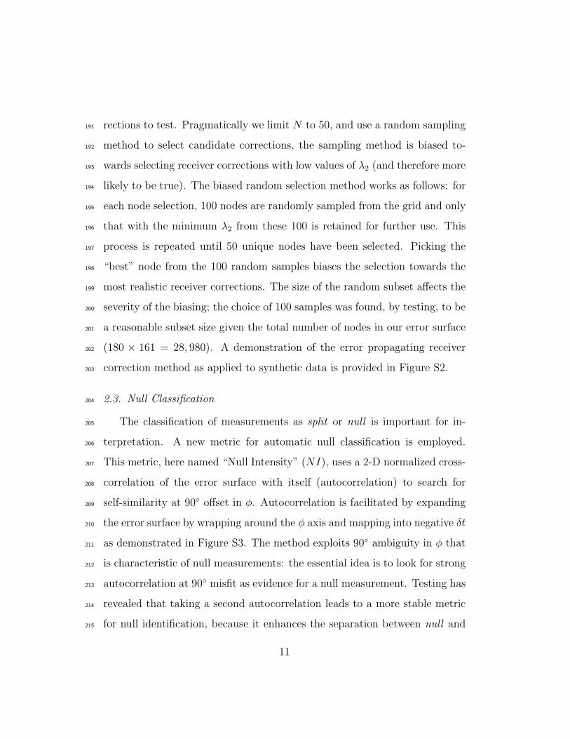
4.1. Delay Times250
Delay times (�t) measure a combination of anisotropy strength and path251
length through the anisotropic region. Figure 2A shows the variation in �t252
with depth for all split (non-null) measurements.253
To first order �t values decline with source depth (Fig 2A). Median �t,254
hereafter e�t, drops from 1.7 s in the 0–50 km depth bin to 1.3 s in the 200–255
250 km depth bin: a decrease of 0.4 s over a depth change of 200 km. This256
drop is strong evidence for the presence of anisotropy above 200 km. One257
could explain 1.7 s of splitting by a 380 km path length through a region of258
2% anisotropy (though due to the tradeo↵ of path length with anisotropy259
strength other solutions are possible, e.g., 260 km through a region of 3%).260
Assuming a simple dipping layer geometry this would correspond to a layer261
thickness of about 290 km (or 200 km with 3% anisotropy). This calcula-262
tion assumes that rays propagate along a path ⇠ 40� incident from the slab263
13
0
100
200
300
400
500
600
700
Sour
ce d
epth
(km
)
0 1 2 3 4δt (s)
100
101
102
No.
# M
easu
rem
ents
0
100
200
300
400
500
600
700
0
100
200
300
400
500
600
700
1 10 100 1000No.# Measurements
0
100
200
300
400
500
600
700
0
100
200
300
400
500
600
700
0 25 50 75 100Percent Null
A. B. C.
Figure 2: A. Global 2-D histogram of split measurement delay times, �t, against source
depth in 0.2 s by 50 km bins; median �t symbols plotted on top with 95% confidence in-
tervals calculated by bootstrapping. Copper colours show the number of measurements
within a bin according to the inset logarithmic colour scale; grey background colour indi-
cates no measurement within bin. B. Total number of measurements – split and null –
for each depth. C. Percentage of null measurements for each depth with 95% confidence
intervals calculated by bootstrapping.
14

normal vector, which is typical within the dataset. The smooth decrease in264
e�t with depth indicates either a gradual shortening of the path length (e.g.,265
due to thinning of the layer) or weakening of anisotropy with depth. To ex-266
plain 1.3 s of splitting from sources in the depth range 200–250 km requires267
a path length of 290 km through 2% anisotropy (or a path length of 200 km268
through 3% anisotropy). Given a dipping layer this corresponds to inferred269
layer thicknesses of 225 km and 150 km in the cases of 2% and 3% anisotropy270
respectively. Therefore, in the scenario that the anisotropic region is a dip-271
ping layer with strength 2% throughout, the layer thins from 290 km near272
the surface to 225 km beneath ⇠ 200 km depth.273
To within 95% confidence e�t ⇠ 1.3 s over the entire depth range 200–274
600 km. This agrees with results reported in several recent studies employing275
similar methodology (Lynner and Long, 2015; Nowacki et al., 2015; Mohiud-276
din et al., 2015). The apparent lack of depth dependence might indicate the277
mantle is isotropic over this depth range and that all splitting shares a com-278
mon anisotropic source in the deeper mantle. However, observations from279
surface waves, which have good depth resolution, indicate that the transition280
zone (410–660 km) is globally anisotropic with a detectable azimuthal com-281
ponent (Trampert and van Heijst, 2002; Yuan and Beghein, 2013). Therefore282
the lack of depth dependence on e�tmay require a more complex interpretation283
than simple isotropy. One possibility is that anisotropy is present through-284
out the depth range 200–600 km but that interference in the splitting signal285
from multiple regions of anisotropy conspires to produce no apparent depth286
variation in e�t.287
The detection of splitting on the deepest events (deeper than 650 km) is288
15
strong evidence for the presence of anisotropy in the upper lower mantle.289
Splitting delay times of ⇠ 1 s require a path length of 300 km through a290
region with 2% anisotropy; assuming a dipping layer geometry such a layer291
would need to be about 180 km thick. This calculation assumes that rays292
propagate along a path ⇠ 50� incident from the slab normal vector, which is293
representative of our data at this depth.294
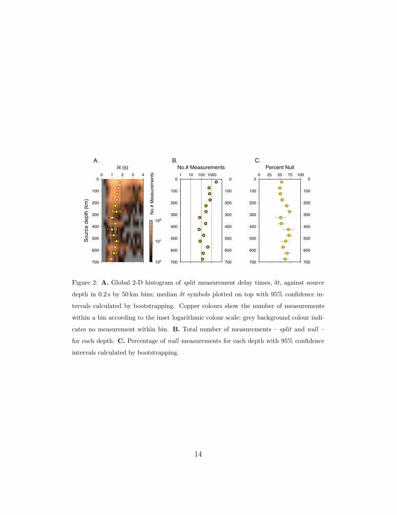
4.2. Fast Directions295
Previous observations of trench parallel fast directions have been used to296
support the sub-slab asthenospheric trench parallel flow hypothesis (Russo297
and Silver, 1994; Long and Silver, 2008, 2009). Figure 3A shows the global298
distribution in the fast wave polarisation direction as projected in the geo-299
graphical reference frame at source location (�src, measured in degrees clock-300
wise from north) coloured by misfit from the local strike of the subducting301
slab (using model Slab1.0; Hayes et al., 2012). There is a large degree of local302
variability in �src (e.g., in the South American and Japan-Kuril subduction303
systems, Fig 3A) demonstrating that trench parallel fast directions are far304
from ubiquitous, though they are slightly more prominent than non-trench-305
parallel observations (Fig 3B). Variability has previously been attributed to306
heterogeneity in the sub-slab mantle or systematic variations due to ray az-307
imuth and takeo↵ angles relative to the dip and strike of the slab caused by308
the style of anisotropy (Song and Kawakatsu, 2012). It is worth noting that309
the number of trench parallel observations is increased significantly if only310
considering events sourced in the upper 50 km (Fig S9).311
Regional plots of each subduction zone considered in this study are pre-312
sented in supplementary figures S10 – S19. These plots show the geographical313
16

φsrc from events 50−250 km deep
0 30 60 90
φsrc misfit from slab strike (°)
0
100
No.
# M
easu
rem
ents
0 30 60 90
φsrc misfit from slab strike (°)
A. B.
Figure 3: A. Map of �src measurements from sources in the depth range 50–250 km;
coloured by misfit from slab strike parallel (approximately trench parallel): blue symbols
are parallel – and red symbols normal – to strike. B. Histogram of �src misfit from slab
strike parallel. Despite a large degree of variation, strike parallel measurements are slightly
more frequent than any other measured orientation. Orientations in the source frame are
calculated according to the equation: �src = ↵+ � � �rcv; where ↵ is azimuth, � is back
azimuth, and �rcv is the fast direction, measured clockwise from north, at the seismic
station.
17

distribution of measurements projected into the source reference frame with314
�src measured from geographical north. This projection assumes a vertical315
ray and therefore does not capture variability with takeo↵ angle or azimuth.316
In order to demonstrate such variability the source frame maps are accom-317
panied by polar panels showing the measurements separated by azimuth and318
takeo↵ angle and the fast direction measured from the projection of the319
vertical direction on the sphere, �ray (vertically polarised ‘SV’ waves have320
�ray = 0� and correspond to radial lines on these plots).321
To investigate the possibility that splitting varies systematically with322
sampling geometry in a globally consistent way we use the slab reference323
frame (Nowacki et al., 2015). This reference frame accounts for variations in324
the ray path in relation to the dip and strike of the subducting slab provid-325
ing a convenient way to incorporate the entire global dataset into a single326
analysis. The slab frame has three orthogonal axes forming a right-handed327
co-ordinate system: strike = 1; dip = 3; and slab normal = 2 (Fig 4A).328
Azimuths are measured clockwise from strike (1) and takeo↵ angles are mea-329
sured relative to the dip vector (3). Note that if the slab has very shallow330
dip then it is possible that rays may take o↵ at angles greater than 90� from331
the dip vector and hence our plots extend to incorporate takeo↵ angles of up332
to 120�. The fast direction, �slab, is measured relative to the projection of333
the slab dip vector (3) on the sphere. If �slab = 0� then the fast shear wave334
is polarised parallel to slab-dip and we will refer to these measurements as335
‘dip parallel’ (in an analogous way to SV waves being polarised parallel to336
the vertical direction); if �slab = ±90� then the fast shear wave is polarised337
normal to slab-dip and we will refer to these measurements as ‘dip normal’338
18

(in an analogous way to SH waves being polarised normal to the vertical339
direction).340
Despite the predominant use of ‘trench parallel’ as a reference orientation341
for describing fast directions in the preexisting literature, we find it more342
useful to describe our slab frame data in terms of ‘dip parallel’, this is natural343
in the slab frame as �slab is measured relative to the projection of the dip344
vector on the sphere. In principle one could measure the fast direction in345
relation to the projection of the strike axis (1) on the sphere and this would346
facilitate description in terms of ‘trench parallel’. One can do this visually347
by checking that the orientation of the bar points towards the strike axis (1);348
e.g., the model shown in Fig 4C predicts trench parallel measurements at349
every sampling angle.350
In Figure 4B–D we show a handful of simple tilted transverse isotropy351
(TTI) models in the slab reference frame. These models act as simple ana-352
logues for a range of plausible anisotropic scenarios in the subslab mantle353
and these are discussed briefly in the figure caption. In Figure 5 a further354
selection of models is shown within the slab reference frame. Models H and I355
are relevant to anisotropy in the upper lower mantle and the lithosphere re-356
spectively. We will compare our data to these models in order to gain insight357
into the nature of anisotropy in the mantle beneath subduction zones.358
In Figure 6 we plot the global dataset in the slab reference frame with359
colours used to emphasise the orientation change in the fast shear wave polar-360
isation direction. The contribution towards the global coverage from di↵erent361
geographic regions is shown in the bottom row of panels in this figure. We362
observe that variability in the fast direction becomes systematically organ-363
19

ised in the slab frame whereby dip normal �slab measurements cluster at364
azimuths normal to slab strike and dip perpendicular �slab measurements365
cluster at oblique azimuths. This basic pattern is seen over the full range366
of source depths with the exception of the deepest events where coverage367
at azimuths normal to slab strike is poor (Fig 6D). It reveals a systematic368
globally consistent nature of anisotropy in the sub-slab mantle controlled369
fundamentally by the overlying slab.370
To extract a global representation of this splitting pattern for a series of371
source depth ranges we calculate the circular mean of �slab and median of �t372
within equal area bins over the sphere (Fig 7). In doing so we assume mirror373
symmetry about the plane normal to strike enabling us to confine almost all374
sub-slab measurements to a quadrant of the hemisphere. To test hypothetical375
models of sub-slab anisotropy the observed pattern can be compared to the376
expected patterns of candidate models (i.e. compare results in Fig 7 to377
models in Figs 4 and 5).378
4.2.1. 50 to 250 km deep sources379
We primarily concentrate on data from sources 50 to 250 km deep; this380
range is chosen to focus on the asthenospheric sub-slab mantle whilst avoid-381
ing bias from the overwhelming number of shallow events in the dataset.382
In Figure 8 we show the di↵erence in �slab between candidate models and383
our averaged representative observations over the sampled range of angles384
in the slab frame. The models that best replicate our �slab pattern are the385
TTI slab normal model (Fig 8D) and the orthorhombic model of Song and386
Kawakatsu (2012) (Fig 8G). The TTI slab normal model is a simple case of387
elliptical anisotropy, with a slow symmetry axis, defined by the Thomsen pa-388
20

D.
B.
Slow Symmetry Axis
TTI slab normale.g. layers
Fast Symmetry Axis
TTI dip parallele.g. entrained flow LPO A-type fabric (approx.)
−180˚
−150˚
−120˚
−90˚
−60˚
−30˚
0˚30˚
60˚
90˚
120˚
150˚
90°
90°
90°Takeoff
Above SlabBelow Slab
Slab
Pla
ne
01234567891011
Anis
otro
py S
treng
th (%
)
DIP
STRIKE
ray
SLAB
1
3
A.
STRIKE
DIP
ABOVE SLABBELOW SLAB
3
−180˚
−150˚
−120˚
−90˚
−60˚
−30˚
0˚30˚
60˚
90˚
120˚
150˚
90°
90°
90°Takeoff
Above SlabBelow Slab
Slab
Pla
ne
01234567891011
Anis
otro
py S
treng
th (%
)
C.
Fast Symmetry Axis
HTI strike parallele.g. trench parallel flow LPO A-type fabric (approx.)(compare with E.)
21
2
ray
−180˚
−150˚
−120˚
−90˚
−60˚
−30˚
0˚30˚
60˚90˚
120˚
150˚
90°
90°
90°Takeoff
Above SlabBelow Slab
Slab
Pla
ne
01234567891011
Anis
otro
py S
treng
th (%
)
Figure 4: A. (left) Sketch of the slab reference frame projected on to a polar grid with
radial direction corresponding to ray takeo↵ angle as measured from the dip vector (3-axis
directed down into the centre of the polar grid) and tangential direction corresponding to
ray azimuth as measured from the strike vector (1-axis). The region left of the vertical
line that defines the plane normal to 2 (i.e. the slab plane) contains all rays that exit
beneath the slab and likewise right of this line rays would exit above the slab; rays situated
along this line have long slab paths. A ray taking o↵ at 60� from the dip vector at an
azimuth �120� from strike is plotted as a red dot. (right) Natural perspective of the slab
frame (wireframe mesh) with the familiar ray this time shown as a red arrow shooting
down beneath the slab. Notice that the grid extends to takeo↵ angles up to 120�; these
angles are necessary as they are occasionally sampled in situations where the slab dip
is very shallow. B. Demonstration of a simple tilted transverse isotropy (TTI) model
with fast symmetry axis parallel to the slab dip vector. The small black bars show the fast
polarisation direction �slab pointing radially (parallel to the symmetry axis) at all locations
with colour showing that anisotropy is strongest at angles normal to the symmetry axis
and weakest at angles parallel to the symmetry axis. This model is analogous to the case
of olivine A-type fabric entrained by subduction. C. Similar to (B.) except the symmetry
axis is pointing parallel to the strike vector; this case is analogous to olivine A-type fabric
oriented trench parallel. D. Similar to (B.) and (C.) except the TTI model has a slow
symmetry axis which points normal to the slab plane; this case is analogous to fine layers
dipping parallel to the slab. Elastic constants for all models given in supplementary Table
S1.
21

E.Olivine A-typeTrench Parallel Flow(Ismail and Mainprice, 1998) F.
Olivine B-typeEntrained Flow(Lee and Jung, 2015) G.
Synthetic OrthorhombicEntrained Flow(Song and Kawakatsu, 2012)
H.Bridgmanite (38 Gpa, 945 km)Entrained Flow(Mainprice et al., 2008)
−180˚
−150˚
−120˚
−90˚
−60˚
−30˚
0˚30˚
60˚
90˚
120˚
150˚
90°90
°
90°Takeoff
Above SlabBelow Slab
Slab
Pla
ne
0
1
2
3
4
5
6
Anis
otro
py S
treng
th (%
)
I.Lithospheric cracks/faultsSlab bending(Tandon and Weng, 1984)
−180˚
−150˚
−120˚
−90˚
−60˚
−30˚
0˚30˚
60˚
90˚
120˚
150˚
90°
90°
90°Takeoff
Above SlabBelow Slab
Slab
Pla
ne
01234567891011
Anis
otro
py S
treng
th (%
)
−180˚
−150˚
−120˚
−90˚
−60˚
−30˚
0˚30˚
60˚
90˚
120˚
150˚
90°
90°
90°Takeoff
Above SlabBelow Slab
Slab
Pla
ne
0
1
2
3
4
5
Anis
otro
py S
treng
th (%
)
−180˚
−150˚
−120˚
−90˚
−60˚
−30˚
0˚30˚
60˚
90˚
120˚
150˚
90°
90°
90°Takeoff
Above SlabBelow Slab
Slab
Pla
ne
0
1
2
3
Anis
otro
py S
treng
th (%
)
−180˚
−150˚
−120˚
−90˚
−60˚
−30˚
0˚30˚
60˚
90˚
120˚
150˚
90°
90°
90°Takeoff
Above SlabBelow Slab
Slab
Pla
ne
0
1
2
3
4
5
6
7
Anis
otro
py S
treng
th (%
)Figure 5: Selection of elastic models in the slab reference frame. E. A-type fabric average
from a database of natural olivine fabrics (Ben Ismail and Mainprice, 1998) rotated with
foliation plane parallel to the slab plane and lineation parallel to strike vector (trench par-
allel flow; cf. Fig 4C). F. B-type natural olivine fabric (Lee and Jung, 2015) with foliation
plane parallel to slab and lineation parallel to dip vector (entrained flow). G. Orthorhom-
bic model of Song and Kawakatsu (2012) combining elements of models B and D (Fig 4).
H. Lower mantle bridgmanite texture (Mainprice et al., 2008) rotated with foliation par-
allel to slab and lineation parallel to dip vector (entrained flow; crystallographic texture
calculated at 30GPa under simple shear deformation with a strain of 2.0 and single crystal
elastic constants calculated at 1500K and 38GPa). I. Cracks/faults dipping at 60� within
the slab (angle measured from horizontal if the slab were flat, the slab frame naturally
accounts for any extra tilting of the slab); modelled using the e↵ective medium theory of
Tandon and Weng (1984). Elastic constants for all models given in supplementary Table
S1.
22

A. 0−50 km B. 50−250 km C. 250−550 km D. 550−700 km
0
30
60
90
φ sla
b (°)
dip normal
dip parallel
South America
Japan−Kuril
Tonga−Kermadec
Figure 6: Top row: Splitting in the slab reference frame for the global dataset separated
by source depth (consult Fig 4 for explanation of this reference frame). Fast direction,
�slab, shown by orientation and colour of bar symbols. Red bars are parallel to the slab
dip vector, blue bars are normal to this direction. Length of bar corresponds to �t with the
longest bars equalling 4 s of splitting. We note good separation of dip normal (blue) and
dip parallel (red) �slab measurements in this reference frame. Bottom row: Constitution
of the global dataset broken down into three broad regions:– red – mainly from the South
American subduction system with minor contributions from the Cascadian, Mexican, and
Scotian systems;– yellow – mainly from the Japan-Kuril subduction system with contri-
butions from the Izu-Bonin-Mariana, Ryukyuan, and Aleutian systems;– blue – mainly
from the Tonga-Kermadec subduction system with contributions from the Indonesian,
Philippine, Solomon, and Vanuatuan systems.
23

−9
0˚
−60˚
−30˚0˚
0
30
60
90
120
Ta
keo
ff A
ng
le
Azimuth
−9
0˚
−60˚
−30˚0˚
0
30
60
90
120
Ta
keo
ff A
ng
le
Azimuth
−9
0˚
−60˚
−30˚0˚
0
30
60
90
120
Ta
keo
ff A
ng
le
Azimuth
−9
0˚
−60˚
−30˚0˚
0
30
60
90
120
Ta
keo
ff A
ng
le
Azimuth
−9
0˚
−60˚
−30˚0˚
0
30
60
90
120
Ta
keo
ff A
ng
le
Azimuth
−9
0˚
−60˚
−30˚0˚
030
60
90
120
Ta
keo
ff A
ng
le
Azimuth
−9
0˚
−60˚
−30˚0˚
0
30
60
90
120
Ta
keo
ff A
ng
le
Azimuth
−9
0˚
−60˚
−30˚0˚
0
30
60
90
120
Ta
keo
ff A
ng
le
Azimuth
55
0−
700
km
250
−5
50 k
m5
0−
250
km
0−
50
km
A. Binned Measurements B. Percentage Null
1.2 1.8 2.4
δt (s)
0 25 50 75 100
Null Measurements (%)
Figure 7: A. Averaging of the slab frame measurements shown in Figure 6. Circular mean
�slab and median �t are calculated within equal area triangular bins for a range of source
depths (indicated on the left). Only bins containing at least 4 measurements and standard
errors of less than 20� in �slab and 0.8 s in �t (calculated by bootstrapping) are shown. B.
Percentage of null measurements detected within each bin. Only bins containing at least 4
measurements and standard error less than 15% (calculated by bootstrapping) are shown.24

rameters � = ✏ = � = 0.1 (Thomsen, 1986). The latter orthorhombic model389
essentially embellishes the former TTI model with a component of azimuthal390
anisotropy in the direction of plate movement to represent the observed az-391
imuthal anisotropy in the asthenosphere (Song and Kawakatsu, 2012). We392
are not able to distinguish between these models due to a gap in coverage393
where the main di↵erence would manifest (azimuth �90� and takeo↵ angle394
90�, relative to the strike and dip vectors of the slab respectively); these395
angles are covered by steeply incident phases (e.g. SKS) on shallow dip-396
ping slabs (Song and Kawakatsu, 2012, 2013). Trench-parallel flow models397
strongly misfit the observations at azimuths ⇠ �60� and takeo↵ angles ⇠ 90�398
(Figs 8C and E); similarly the entrained B-type model also misfits at these399
angles (Fig 8F). This is evidence that trench parallel flow is not likely to be400
a dominant mode of material transport in the sub-slab mantle (the same ar-401
gument rules out the entrained B-type model). By similar argument: misfit402
at azimuths ⇠ �90� rules out the entrained olivine A-type model (Fig 8B).403
Olivine C-type and E-type fabrics are more likely to exist in the astheno-404
sphere than A-type fabric (Karato et al., 2008); we notice the character of405
the splitting pattern associated with these fabrics is qualitatively similar to406
A-type fabrics (Fig S21) such that they can be reasonably well approximated407
by hexagonal symmetry with a fast symmetry axis. Our data seem to require408
a slow symmetry axis and therefore C- and E-type fabrics are not compatible409
with our observations.410
To investigate the extent to which this global observation holds in sep-411
arate regions we consider the percentage of measurements that fit a given412
model for each subduction zone. To do this each fast direction measure-413
25

ment is modelled as a wrapped gaussian function (180 degree periodicity),414
normalised so that the area under the curve equals one, and with a width415
and height determined by the errors in the measurement and a peak location416
corresponding to the angular misfit from the model predicted fast direction.417
The ensemble of all measurements (i.e. gaussians) for a particular region418
is then stacked and renormalised so that the area under the curve is equal419
to one hundred. The resultant curve is a kernel density estimation (KDE;420
Parzen, 1962) showing the distribution in misfit between the data and the421
model. Such a curve can be considered as a smooth histogram. The area422
under the curve in the interval -30 to 30 degrees represents the percentage of423
measurements that fit the model (fast directions) within 30 degrees. Figure424
S22 shows the KDE misfit curves for a selection of the best sampled regions425
for both the slab normal model (left panel) and the trench parallel model426
(right panel). The area beneath these curves in the interval -30 to 30 degrees427
for each region is tabulated in Table S2.428
Generally speaking the slab normal model performs better than the trench429
parallel model for the majority of regions as shown by the higher percentage430
of measurements within the±30� interval. This is especially true of the South431
American and Honshu-Kuril regions where the high number of measurements432
indicates statistical significance. These regions are the best sampled regions433
in the dataset not simply because of their high number of measurements but434
also because they contain ray coverage at a wide range of sampling angles.435
Importantly, in both these region there is sampling at the key angle around436
�60� azimuth and 75� takeo↵ in the slab reference frame where the di↵erence437
between the slab normal and trench parallel models is clearest (Fig S20). The438
26

Tonga-Kermadec subduction zone is anomalous in that the trench parallel439
model appears to fit better than the slab normal model. This subduction440
zone is notable for strong trench roll-back in the north (from where most441
measurements are obtained) perhaps associated with an abnormal sub-slab442
mantle flow. However, though this region yields a good number of mea-443
surements, the slab frame coverage is limited at the key angles needed to444
most clearly distinguish between the trench parallel and slab normal mod-445
els (Fig S20). In the Aleutia-Alaska, Izu-Bonin-Mariana, Ryukyu, Solomon,446
and Vanuatan regions the slab normal and trench parallel models perform447
similarly. This is not surprising as the coverage in these regions is limited to448
angles at which both models predict similar fast directions (Fig S20). The449
Philippine, Central America, Sandwich, and Indonesian regions are limited450
by a low number of measurements and therefore we do not comment on these.451
In summary the slab normal model is clearly better than the trench par-452
allel model beneath South America and the Honshu-Kuril subduction zones,453
but not beneath the Tonga-Kermadec system (though this region lacks key454
coverage at the most diagnostic slab frame angles). In other regions coverage455
is not su�cient to strongly prefer one model over the other. Therefore we can456
rule out large scale trench-parallel flow beneath the best sampled subduction457
zones: South America and the Honshu-Kuril. Though previous workers have458
inferred trench parallel flow beneath some subduction zones, this was largely459
based on map views of the data which fail to capture variations in splitting460
due to changes in sampling angles. From our dataset (which considers the461
geometrical sampling variations in the slab reference frame) we do not see462
compelling evidence to prefer the trench parallel model for any particular463
27

subduction zone system.464
4.2.2. 0 to 50 km deep sources465
Measurements from events shallower than 50 km show a slightly di↵erent466
pattern with an average slab-normal �slab detected on rays around azimuth467
�60� and takeo↵ angle 60� from the strike and dip of the slab respectively468
(Figs 6 and 7). Note that these measurements appear parallel to the sub-469
duction zone trench when viewed in the geographical reference frame (Fig470
S9). This suggests the existence of a distinct region of anisotropy in the471
upper ⇠ 50 km (and therefore within the lithospheric slab). No model per-472
fectly replicates the splitting pattern over the whole range of angles. Though473
any signal from the shallow anisotropic region would be contaminated by474
anisotropy in deeper regions obscuring its true nature; therefore we cannot475
directly compare models with the data. With that caveat, it is interesting to476
note that the slab normal �slab observations around azimuth �60� and take-477
o↵ angle 60� are consistent with the pattern expected from the HTI strike478
parallel model (Fig S23C); alternatively, a tilting of the slow symmetry axis479
model (Fig 4D) so that the axis points down the dip vector of the slab would480
also produce this pattern. Faults within the slab would be expected to create481
an SPO fabric that would fit the data reasonably well (Fig S24).482
4.2.3. 250 to 550 km deep sources483
Fast directions, �slab, from sources in the depth range 250–550 km are484
not neatly compatible with any of the candidate models considered in Fig-485
ure S25. There is an approximate fit to the TTI model that we favour to486
explain the shallower 50–250 km source depth data (Fig S25D). This may487
28

B. TTI down dip
−9
0˚
−60˚
−30˚0˚
0
30
60
90
120
Ta
keo
ff A
ng
le
Azimuth
C. HTI along strike
−9
0˚
−60˚
−30˚0˚
0
30
60
90
120
Ta
keo
ff A
ng
le
Azimuth
D. TTI slab normal
−9
0˚
−60˚
−30˚0˚
0
30
60
90
120
Ta
keo
ff A
ng
le
Azimuth
E. Olivine A−type
−9
0˚
−60˚
−30˚0˚
0
30
60
90
120
Ta
keo
ff A
ng
le
Azimuth
F. Olivine B−type
−9
0˚
−60˚
−30˚0˚
0
30
60
90
120
Ta
keo
ff A
ng
le
Azimuth
G. Ortho. (SK2012)
−9
0˚
−60˚
−30˚0˚
0
30
60
90
120
Ta
keo
ff A
ng
le
Azimuth
Model Misfits 50−250 km
0
30
60
90
An
gu
lar
Mis
fit (
°)
Figure 8: Comparison of averaged �slab observations (from sources in the depth range 50
to 250 km, Fig 7) to the predictions of models in Figure 4 (hence labels start from B).
This depth range most directly probes anisotropy in the asthenospheric sub-slab mantle.
Black ticks show the predicted orientation of �slab according to the model; yellow ticks
the observed measurement; background colour indicates the angular misfit between these
two orientations: cyan colours indicate good fit while magenta colours indicate poor fit.
Model B (TTI with symmetry axis pointing down dip of the slab, analogue for olivine
A-type under entrained flow,) strongly misfits the data at azimuths normal to the slab
though is more compatible at oblique angles. Model C (HTI with symmetry axis pointing
along strike, analogue for olivine A-type under trench parallel flow,) fits well for rays with
azimuths close to slab normal but fails at oblique angles. Model D (TTI with symmetry
axis pointing normal to the slab) fits the data well over a wide range of angles. Models E
and F are similar to model C; model G is similar to model D. Refer to Figure 4 for more
detailed information about the models.
29

hint that the above layer extends to deeper depths and misfit is caused by488
increasing interference with deeper regions of anisotropy. However, if these489
measurements are sensitive to more than one layer of anisotropy then a more490
complex analysis is required to interpret these results.491
4.2.4. Deeper than 550 km sources492
Measurements from sources deeper than 550 km, on average, best fit the493
model of entrained bridgmanite, though only a small amount of coverage is494
available (Fig S26H). This model is derived from a texture model simulated495
at 30GPa (⇠850 km depth) deformed under simple shear with strain of 2.0496
and elastic constants calculated at pressure and temperature of 38GPa and497
1500K (Mainprice et al., 2008). The entrained bridgmanite model predicts498
that the strength of anisotropy, at the angles sampled in our dataset, is ⇠ 2%.499
From this we infer a sheared layer thickness of ⇠ 180 km (as discussed earlier500
to explain delay times of ⇠ 1 s). A recently published experimentally derived501
model of deformed bridgmanite (Tsujino et al., 2016) fits the data very well502
Fig S27.503
4.3. Null Measurements504
Null measurements are those with �t below the resolution of the data505
(⇠ 0.4 s; note lack of measurements below 0.4 s in the “�t (s)” histogram in506
Fig S8). The percentage of null measurements in the dataset varies between507
50% and 70% tending to increase with source depth (Fig 2C). The large508
percentage of null measurements requires some explanation. It is important509
to recognise that these observations do not necessarily imply an isotropic510
region. Null measurements can occur for a number of reasons:511
30

• because anisotropy is locally very weak or isotropic;512
• the wave is sampling along an isotropic direction (e.g., the symmetry513
axis of a transverse isotropic medium);514
• the wave is polarised in the fast or slow direction;515
• multiple regions of anisotropy cancel one another out.516
The most noteworthy feature of the null measurements is that their oc-517
currence depends strongly on the ray takeo↵ angle in the slab reference frame518
(Fig 9). Rays sourced in the upper 350 km (excluding the shallowest 50 km)519
yield fewer null measurements (as a percentage) when propagating down the520
dip vector of the slab than when travelling normal to the slab plane (Fig 7B).521
This may be due to the heterogeneity of the slab itself or it may be due to522
the style of anisotropy. A TTI medium with symmetry axis pointing normal523
to the slab could explain this observation because waves travelling down the524
symmetry axis of such a medium would not split. A TTI model can thus525
explain both the patterns in null concentrations and the fast directions.526
The opposite dependence of null measurements on ray takeo↵ angle is527
true for deeper sourced rays (sourced deeper than 350 km): rays propagating528
down the dip vector of the slab yield more null measurements than those529
travelling at angles o↵set from this axis (Fig 9). It is possible that the530
slab itself provides an (apparently) isotropic pathway in the deep mantle.531
Alternatively this could be explained by a TTI medium with symmetry axis532
pointing in the slab dip direction. Note, however, that the favoured entrained533
bridgmanite model (Fig 4H) does not predict this observed pattern in null534
measurements: it predicts reasonably strong splitting for rays travelling in535
31

the down slab dip direction. However, all rays in the dataset that propagate536
down the slab are derived from sources shallower than 550 km (Fig 7B).537
This feature cannot therefore be ascribed with confidence to anisotropy in538
the upper lower mantle (below 660 km –where bridgmanite exists); it allows539
the possibility that two-layer interference between a lower transition zone540
layer (in the depth range 550–660 km) and the upper lower mantle gives rise541
to the abundance of null measurements seen at this angle – this would require542
that the two layers systematically cancel one-another out.543
5. Conceptual Model544
A conceptual model of anisotropy beneath a subduction zone inferred545
from the key features of the dataset is presented in the cartoon of Figure546
10. Here we discuss how our observations justify that model followed by547
a discussion of the possible causes of anisotropy. Working downwards with548
depth, our conceptual model consists of the following regions of anisotropy:549
1. Lithosphere: Despite a wealth of data from shallow events the interpre-550
tation of anisotropy in the lithosphere is apparently compromised by551
interference in the signal from anisotropy in the deeper mantle. Never-552
theless a change in fast direction observed with change in source depth –553
above and below 50 km – indicates the presence of a distinct lithospheric554
region of anisotropy. Shallow sourced measurements tend to appear555
parallel to the subduction zone trench when viewed in the geograph-556
ical reference frame, suggesting that previous reports of widespread557
trench parallel anisotropy may be biased by the great number of shal-558
low events. The fact that this signal is unique to shallow source data559
32

0
25
50
75
100
Perc
enta
ge N
ull (
%)
0 30 60 90Takeoff Angle (from slab dip vector) (°)
Shallow Events (50−350 km)Deep Events (350−700 km)
Figure 9: Percentage of null measurements as a function of ray takeo↵ angle (measured
from slab dip vector). Data are divided into shallow (50–350 km, yellow) and deep sources
(350–700 km, blue). Error bars are one standard deviation of 1000 untrimmed bootstrap
samples (Efron and Tibshirani, 1991). We note the percentage of null measurements
increases with takeo↵ angle for shallow sources and decreases with takeo↵ angle for deep
sources.
33

(shallower than 50 km depth) implies that this anisotropy does not sur-560
vive deep subduction.561
2. Asthenosphere: The steady reduction in �t with increasing source depth562
is strong evidence for the presence of anisotropy in the upper ⇠200 km.563
Assuming 2% anisotropy and dipping layer geometry the anisotropic564
layer thins from 290 km near the surface to 225 km upon subduction565
to depths beyond ⇠ 200 km. Alternatively the strength of anisotropy566
weakens with depth. In either case we infer that this layer may exist567
to depths in excess of 400 km. The pattern in �slab strongly resembles568
that expected from a TTI medium (Fig 8D) with a slow symmetry axis569
pointing subnormal to the plane of the subducting slab. Moreover the570
concentration of null measurements increases as rays propagate closer571
to this proposed symmetry axis (as expected for a TTI medium). These572
results are compatible with the strong radial anisotropy model of Song573
and Kawakatsu (2012).574
The previous study of Lynner and Long (2014b) employed similar575
methodology to this study but came to di↵erent conclusions concern-576
ing the validity of the strong radial anisotropy model of Song and577
Kawakatsu (2012). They found the model to be broadly incompati-578
ble with their data. Instead they favoured an age dependent model579
whereby systems with young lithosphere exhibit splitting aligned with580
absolute plate motion and systems with older lithosphere (> 95Ma)581
exhibit splitting parallel to the subduction zone trench. Evidence that582
our results di↵er from those of Lynner and Long (2014b) comes from583
inspecting histograms of �slab misfit from trench parallel: in our study584
34

the histogram shows more ‘trench-parallel’ results (Fig 2B) than the585
corresponding histogram in their study (their Fig 4A); though neither586
study shows a particularly strong dependence of fast direction on the587
trench orientation. Di↵erences between the two studies may arise due588
to di↵erences in data coverage and methodology. Our conclusions may589
also di↵er due to our use of the slab reference frame in the analysis590
stage.591
3. Transition zone: A lack of depth dependence on �t from sources in the592
depth range 250–550 km is compatible with isotropy in this depth range.593
However, we do not conclude that the transition zone is isotropic as the594
interference between multiple regions of anisotropy could also explain595
this observation. Interpretation in this depth range is compromised by596
a paucity of data and the potential for interference between multiple597
regions of anisotropy, therefore we resist commenting further.598
4. Upper lower mantle: Splitting observed on events deeper than 660 km599
is strong evidence for the presence of anisotropy in the upper lower600
mantle. To explain the observed �t values of ⇠ 1 s requires a layer601
of 2% anisotropy ⇠ 180 km thick. On average �slab is parallel to the602
dip direction of the slab resembling a TTI style of anisotropy with603
fast symmetry axis pointing in the slab dip direction. Furthermore,604
the concentration of null measurements increases as rays propagate605
closer to the slab dip direction, as would be expected for this style of606
anisotropy.607
35

0
100
200
300
400
500
600
700
slow axis TTIanisotropy
fast axisTTI anisotropy
δt = 1.7 s
δt = 1.5 s
δt ~ 1 s
complex signal
Depth (km)
δt = 1.3 s
nulls
nulls
1. Lithosphere
2. Asthenosphere
3. TransitionZone
4. Upper Lower Mantle
Figure 10: Conceptual model of anisotropy in the sub-slab mantle. 1. Lithosphere:
unusually high frequency of trench parallel observations from sources in upper 50 km, pos-
sibly caused by SPO of trench parallel faults, though interference expected from deeper
layers clouds interpretation. 2. Asthenosphere: dependence on fast direction with
takeo↵ angle and azimuth relative to dip and strike of the slab is consistent with that ex-
pected from a TTI medium with slow symmetry axis pointing subnormal to the slab. Null
measurements are more frequently made on rays travelling along the proposed symmetry
axis. Median delay times decline gradually with source depth from ⇠ 1.7 s for shallower
events (50 km depth) to ⇠ 1.3 s for deeper events (250 km). 3. Transition Zone: no
clearly distinct signal is detected from events in the depth range 250–550 km; this may be
because the number of data from this range is low, or that the signal is contaminated by
the interference of multiple regions of anisotropy. It is interesting that null measurements
become more frequent for rays that shoot down the slab. 4. Upper Lower Mantle:
median delay times ⇠ 1 s from very deep events evidence the presence of anisotropy in
the upper lower mantle; dependence on fast direction with ray angle, and the elevated
occurrence of null measurements down the slab, is consistent with TTI medium with fast
symmetry axis pointing subparallel to the slab dip direction.
36

5.1. Possible causes of anisotropy608
Anisotropy can be caused by the lattice-preferred orientation (LPO) of in-609
trinsically anisotropic crystals and/or the shape-preferred orientation (SPO)610
of elastically heterogeneous features of length scale several times shorter than611
the seismic wavelength. Here we consider the geophysically plausible causes612
of anisotropy within the regions of our conceptual model (Fig 10):613
1. Lithosphere: A simple SPO model of faults in the slab dipping 60� to-614
wards the back arc can potentially explain the wealth of dip-normal615
�slab observations (Fig S24). Such faults are expected to form by616
flexure of the lithosphere upon subduction. Anisotropy of this type617
might be enhanced by the addition of LPO from highly anisotropic hy-618
drous phases such as antigorite and talc (Faccenda et al., 2008). Fossil619
anisotropy in the lithosphere — due to the LPO of olivine crystals620
in the direction of plate motion during formation (e.g., Shearer and621
Orcutt, 1986; Tommasi, 1998) — does not explain our observations be-622
cause this fossil direction does not systematically align parallel to the623
trench of the subduction zone (Long and Silver, 2008).624
2. Asthenosphere: Anisotropy in the peridotitic asthenosphere has widely625
been considered to be caused by the LPO of olivine crystals with a axes626
oriented in the shear direction by dislocation creep deformation (e.g.,627
Nicolas and Christensen, 1987). The resultant A-type fabric explains628
the widespread azimuthal anisotropy observed in surface wave studies629
(e.g., Debayle et al., 2005) and shear wave splitting on SKS phases630
(e.g., Walpole et al., 2014); such fabrics can also potentially explain631
the observed radial anisotropy (Becker et al., 2008). Other types of632
37

fabric are possible and may be present (e.g., Karato et al., 2008). Fab-633
rics with strong radial anisotropy are predicted if deformation occurs in634
the presence of partial melt in the di↵usion creep deformation regime635
(Holtzman et al., 2003; Miyazaki et al., 2013). Fabrics with strong ra-636
dial anisotropy are also predicted if the medium undergoes axial short-637
ening in the vertical direction (Tommasi et al., 1999). Alternatively an638
SPO mechanism might explain the strong radial anisotropy. For exam-639
ple horizontal layers of partial melt could contribute radial anisotropy640
under ‘normal’ oceanic conditions (Kawakatsu et al., 2009); however,641
as noted by Song and Kawakatsu (2012), upon subduction any melt is642
likely to solidify and thereby reduce the strength of this anisotropy. It643
remains to be determined whether the anisotropy we detect is formed in644
the ambient asthenosphere and is tilted in place by subduction (imply-645
ing strong coupling between lithosphere and asthenosphere; Song and646
Kawakatsu, 2012) or whether it is created by the subduction process647
itself.648
3. Transition zone: Given the potential di�culties in confidently inter-649
preting transition zone anisotropy from our dataset we do not com-650
ment on the possible causes of anisotropy. However, previous work has651
suggested the presence of hydrous phases in this region can explain the652
anisotropy (Nowacki et al., 2015), and our results are broadly compat-653
ible with this interpretation.654
4. Upper lower mantle: Bridgmanite is volumetrically the most impor-655
tant mineral, comprising about 70% of the mantle at shallow lower656
mantle depths; this mineral is strongly anisotropic (⇠ 12% shear wave657
38

anisotropy at 660 km depth; Karki, 1999) and is capable of forming658
LPO fabric (Cordier et al., 2004; Wenk et al., 2004). Theoretical work659
suggests that the LPO of bridgmanite produces moderate anisotropy660
(⇠ 2�3% at 38GPa or ⇠ 980 km depth; which would likely be stronger661
at shallower depths; Mainprice et al., 2008). Alternatively an SPO662
mechanism would require tubule (cigar shaped) inclusions elongated in663
the dip direction, these inclusions would likely need to be low velocity664
in order to produce su�ciently strong anisotropy (Kendall and Silver,665
1998).666
6. Conclusions667
In this study we use automation to process a large volume of source-668
side splitting data on teleseismic S phases. A new method is introduced to669
propagate uncertainty in the receiver correction into the error of our mea-670
surements; and a novel null identification method is employed to aid inter-671
pretation. Manually verified quality control reduces the dataset to 6369 high672
quality measurements made from subduction zone earthquake sources. These673
data place constraints on the mineralogy and geodynamics of the sub-slab674
mantle.675
We find that the asthenospheric sub-slab mantle is approximately trans-676
versely isotropic with a slow symmetry axis pointing subnormal to the plane677
of the slab (as recently hypothesized; Song and Kawakatsu, 2012). Assuming678
2% strength the anisotropic layer is ⇠ 300 km thick and thins to ⇠ 200 km679
upon subduction. Alternatively the fabric strength weakens with depth. In680
either case we infer the subduction of this fabric to transition zone depths.681
39
Either strong radially anisotropic fabric developed in the asthenosphere un-682
der ‘normal’ conditions is tilted by the subduction process and carried down683
to transition zone depths or the fabric is created by the subduction process684
itself. Strong radially anisotropic fabrics in peridotite can be created by ax-685
ial shortening in the vertical direction, or di↵usion creep deformation in the686
presence of partial melt; fabric created by dislocation creep in olivine might687
also produce su�cient radial anisotropy, though we do not have su�cient688
coverage at the necessary angles to detect the expected azimuthal anisotropy689
in this case. Our results are incompatible with previously suggested models690
involving trench parallel flow, raising doubt over its widespread occurrence.691
An abundance of ‘trench parallel’ splitting is measured on the shallowest692
data (from sources in the upper 50 km) suggesting a unique style of anisotropy693
contained in the slab. This anisotropy could be caused by the shape preferred694
orientation of faults formed parallel to the trench by slab bending.695
The upper lower mantle appears approximately transversely isotropy with696
a fast symmetry axis pointing subparallel to the subduction direction. As-697
suming 2% strength the anisotropic layer is ⇠ 200 km thick. The deformation698
of bridgmanite is a plausible candidate mechanism to explain our observa-699
tions.700
7. Acknowledgements701
The research leading to these results has received funding from the Euro-702
pean Research Council under the European Unions Seventh Framework Pro-703
gram (FP7/20072013)/ERC grant agreement 240473 CoMITAC. We thank704
Andy Nowacki for helpful discussions particularly with regards to rotating705
40
the data into the slab reference frame. We also thank two anonymous review-706
ers for helpful comments that improved the manuscript. This work would not707
have been possible without the IRIS DMC data archive. Figures were mostly708
produced using the free Generic Mapping Tools software (GMT) (Wessel and709
Smith, 1991).710
41

Alisic, L., Gurnis, M., Stadler, G., 2012. Multi-scale dynamics and rheology711
of mantle flow with plates. Journal of geophysical Research 117 (B10402).712
Ando, M., Ishikawa, Y., Wada, H., Jul. 1980. S-wave anisotropy in the upper713
mantle under a volcanic area in Japan. Nature 286, 43–46.714
Becker, T. W., Faccenna, C., 2009. A Review of the Role of Subduction715
Dynamics for Regional and Global Plate Motions. In: Subduction Zone716
Geodynamics. Frontiers in earth sciences, Berlin, Heidelberg, pp. 3–34.717
Becker, T. W., Kustowski, B., Ekstrom, G., 2008. Radial seismic anisotropy718
as a constraint for upper mantle rheology. Earth Planet. Sci. Lett.719
Ben Ismail, W., Mainprice, D., Oct. 1998. An olivine fabric database: an720
overview of upper mantle fabrics and seismic anisotropy. Tectonophysics721
296 (1-2), 145–157.722
Bercovici, D., 2003. The generation of plate tectonics from mantle convection.723
Earth Planet. Sci. Lett.724
Billen, M. I., 2008. Modeling the dynamics of subducting slabs. Annu. Rev.725
Earth Pl. Sc.726
Civello, S., 2004. Toroidal mantle flow around the Calabrian slab (Italy) from727
SKS splitting. Geophys. Res. Lett. 31 (10), L10601.728
Cordier, P., Ungar, T., Zsoldos, L., Tichy, G., Apr. 2004. Dislocation creep in729
MgSiO3 perovskite at conditions of the Earth’s uppermost lower mantle.730
Nature 428 (6985), 837–840.731
42

Debayle, E., Kennett, B., Priestley, K., 2005. Global azimuthal seismic732
anisotropy and the unique plate-motion deformation of Australia. Nature733
433, 509–512.734
Di Leo, J. F., Walker, A. M., Li, Z. H., Wookey, J., Ribe, N. M., Kendall,735
J. M., Tommasi, A., 2014. Development of texture and seismic anisotropy736
during the onset of subduction. Geochem. Geophys. Geosyst. 15 (1).737
Di Leo, J. F., Wookey, J., Hammond, J. O. S., Kendall, J. M., Kaneshima,738
S., Inoue, H., Yamashina, T., Harjadi, P., 2012. Deformation and mantle739
flow beneath the Sangihe subduction zone from seismic anisotropy. Phys.740
Earth Planet. Int. 194, 38–54.741
Dziewonski, A. M., Anderson, D. L., 1981. Preliminary reference Earth742
model. Phys. Earth Planet. Int. 25 (4), 297–356.743
Efron, B., Tibshirani, R., 1991. Statistical data analysis in the computer age.744
Science 253 (5018), 390–395.745
Faccenda, M., Burlini, L., Gerya, T. V., Mainprice, D., Oct. 2008. Fault-746
induced seismic anisotropy by hydration in subducting oceanic plates. Na-747
ture 455 (7216), 1097–1100.748
Faccenda, M., Capitanio, F. A., 2012. Development of mantle seismic749
anisotropy during subduction-induced 3-D flow. Geophys. Res. Lett.750
39 (L11305).751
Fischer, K. M., Wiens, D. A., Jul. 1996. The depth distribution of mantle752
anisotropy beneath the Tonga subduction zone. Earth Planet. Sci. Lett.753
142 (1-2), 253–260.754
43

Fouch, M., Fischer, K., 1996. Mantle anisotropy beneath northwest Pacific755
subduction zones. J. Geophys. Res. 101 (B7), 15987–16002.756
Hayes, G. P., Wald, D. J., Johnson, R. L., Jan. 2012. Slab1.0: A three-757
dimensional model of global subduction zone geometries. J. Geophys. Res.758
117 (B01302).759
Holtzman, B. K., Kohlstedt, D. L., Zimmerman, M. E., Heidelbach, F., Hi-760
raga, T., Hustoft, J., Aug. 2003. Melt Segregation and Strain Partitioning:761
Implications for Seismic Anisotropy and Mantle Flow. Science 301 (5637),762
1227–1230.763
Honda, S., 2009. Numerical simulations of mantle flow around slab edges.764
Earth Planet. Sci. Lett. 277, 112–122.765
Houser, C., Masters, G., Shearer, P., Laske, G., 2008. Shear and compres-766
sional velocity models of the mantle from cluster analysis of long-period767
waveforms. Geophys. J. Int. 174, 195–212.768
Jung, H., Katayama, I., Jiang, Z., Hiraga, T., Karato, S., Jul. 2006. E↵ect769
of water and stress on the lattice-preferred orientation of olivine. Tectono-770
physics 421 (1-2), 1–22.771
Jung, H., Mo, W., Green, H. W., Jan. 2009. Upper mantle seismic anisotropy772
resulting from pressure-induced slip transition in olivine. Nature Geosci.773
2 (1), 73–77.774
Kaneshima, S., 2014. Upper bounds of seismic anisotropy in the Tonga slab775
near deep earthquake foci and in the lower mantle. Geophys. J. Int.776
44

Kaneshima, S., Silver, P. G., Dec. 1992. A search for source side mantle777
anisotropy. Geophys. Res. Lett. 19 (10), 1049–1052.778
Karato, S., Jung, H., Katayama, I., Skemer, P., May 2008. Geodynamic779
Significance of Seismic Anisotropy of the Upper Mantle: New Insights780
from Laboratory Studies. Annu. Rev. Earth Pl. Sc. 36 (1), 59–95.781
Karki, B. B., Nov. 1999. First-Principles Determination of Elastic Anisotropy782
and Wave Velocities of MgO at Lower Mantle Conditions. Science783
286 (5445), 1705–1707.784
Kawakatsu, H., Kumar, P., Takei, Y., Shinohara, M., Kanazawa, T.,785
Araki, E., Suyehiro, K., 2009. Seismic Evidence for Sharp Lithosphere-786
Asthenosphere Boundaries of Oceanic Plates. Science 324 (5926), 499–502.787
Kendall, J. M., Silver, P. G., 1998. Investigating causes of D00 anistropy. In:788
The core-mantle boundary region. American Geophysical Union, Washing-789
ton, D. C., pp. 97–118.790
Kincaid, C., 1995. Subduction dynamics: From the trench to the coremantle791
boundary. Rev. Geophys. 33 (S1), 401–412.792
Kincaid, C., Gri�ths, R. W., Sep. 2003. Laboratory models of the thermal793
evolution of the mantle during rollback subduction. Nature 425 (6953),794
58–62.795
Lee, J., Jung, H., Jan. 2015. Lattice-preferred orientation of olivine found in796
diamond-bearing garnet peridotites in Finsch, South Africa and implica-797
tions for seismic anisotropy. Journal of Structural Geology 70, 12–22.798
45

Li, Z. H., Di Leo, J. F., Ribe, N. M., 2014. Subductioninduced mantle flow,799
finite strain, and seismic anisotropy: Numerical modeling. J. Geophys.800
Res. 119 (6), 5052–5076.801
Long, M. D., Silver, P. G., 2008. The subduction zone flow field from seismic802
anisotropy: a global view. Science 319, 315–319.803
Long, M. D., Silver, P. G., 2009. Mantle flow in subduction systems: The804
subslab flow field and implications for mantle dynamics. Journal of geo-805
physical Research 114 (B10312).806
Lowman, J. P., Pinero-Feliciangeli, L. T., Kendall, J. M., Hosein Shah-807
nas, M., 2007. Influence of convergent plate boundaries on upper mantle808
flow and implications for seismic anisotropy. Geochem. Geophys. Geosyst.809
8 (Q08007).810
Lynner, C., Long, M. D., Jan. 2013. Sub-slab seismic anisotropy and mantle811
flow beneath the Caribbean and Scotia subduction zones: E↵ects of slab812
morphology and kinematics. Earth Planet. Sci. Lett. 361, 367–378.813
Lynner, C., Long, M. D., May 2014a. Subslab anisotropy beneath the Suma-814
tra and circum-Pacific subduction zones from source-side shear wave split-815
ting observations. Geochem. Geophys. Geosyst. 15.816
Lynner, C., Long, M. D., 2014b. Testing models of sub-slab anisotropy using817
a global compilation of source-side shear wave splitting data. J. Geophys.818
Res. 119, 7226–7244.819
46

Lynner, C., Long, M. D., 2015. Heterogeneous seismic anisotropy in the tran-820
sition zone and uppermost lower mantle: evidence from South America,821
Izu-Bonin and Japan. Geophys. J. Int.822
Mainprice, D., Tommasi, A., Ferre, D., Carrez, P., Cordier, P., Jul. 2008.823
Predicted glide systems and crystal preferred orientations of polycrys-824
talline silicate Mg-Perovskite at high pressure: Implications for the seismic825
anisotropy in the lower mantle. Earth Planet. Sci. Lett. 271 (1-4), 135–144.826
Meade, C., Silver, P. G., Kaneshima, S., 1995. Laboratory and Seismological827
Observations of Lower Mantle Isotropy. Geophys. Res. Lett. 22 (10), 1293–828
1296.829
Miyazaki, T., Sueyoshi, K., Hiraga, T., Oct. 2013. Olivine crystals align830
during di↵usion creep of Earth’s upper mantle. Nature 502 (7471), 321–831
326.832
Mohiuddin, A., Long, M. D., Lynner, C., Aug. 2015. Mid-mantle seismic833
anisotropy beneath southwestern Pacific subduction systems and implica-834
tions for mid-mantle deformation. Phys. Earth Planet. Int. 245, 1–14.835
Nettles, M., Dziewonski, A. M., 2008. Radially anisotropic shear velocity836
structure of the upper mantle globally and beneath North America. J.837
Geophys. Res. 113 (B02303).838
Nicolas, A., Christensen, N. I., 1987. Formation of anisotropy in upper mantle839
peridotites: A review. Composition.840
47

Nowacki, A., Kendall, J. M., Wookey, J., Feb. 2012. Mantle anisotropy be-841
neath the Earth’s mid-ocean ridges. Earth Planet. Sci. Lett. 317-318, 56–842
67.843
Nowacki, A., Kendall, J. M., Wookey, J., Pemberton, A., Feb. 2015.844
Mid-mantle anisotropy in subduction zones and deep water transport.845
Geochem. Geophys. Geosyst. 16, 764–784.846
Ohuchi, T., Kawazoe, T., Nishihara, Y., Nishiyama, N., Irifune, T., Apr.847
2011. High pressure and temperature fabric transitions in olivine and vari-848
ations in upper mantle seismic anisotropy. Earth Planet. Sci. Lett. 304 (1-849
2), 55–63.850
Paczkowski, K., Montesi, L., Long, M. D., Thissen, C. J., 2014. Three-851
dimensional flow in the subslab mantle. Geochem. Geophys. Geosyst. 15,852
3989–4008.853
Panning, M., Romanowicz, B., 2006. A three-dimensional radially anisotropic854
model of shear velocity in the whole mantle. Geophys. J. Int. 167 (1), 361–855
379.856
Parzen, E., 1962. On Estimation of a Probability Density Function and Mode.857
The Annals of Mathematical Statistics.858
Phipps Morgan, J., Hasenclever, J., Hort, M., Rupke, L., Parmentier, E. M.,859
Jun. 2007. On subducting slab entrainment of buoyant asthenosphere.860
Terra Nova 19 (3), 167–173.861
Restivo, A., Hel↵rich, G., 1999. Teleseismic shear wave splitting measure-862
ments in noisy environments. Geophys. J. Int. 137, 821–830.863
48

Ribe, N., 1992. On the relation between seismic anisotropy and finite strain.864
J. Geophys. Res. 97 (B6), 8737–8747.865
Ribe, N. M., 1989. Seismic anisotropy and mantle flow. J. Geophys. Res.866
94 (B4), 4213–4223.867
Russo, R., Silver, P. G., 1994. Trench-parallel flow beneath the Nazca plate868
from seismic anisotropy. Science 263 (5150), 1105–1111.869
Savage, M., 1999. Seismic anisotropy and mantle deformation: What have870
we learned from shear wave splitting? Rev. Geophys. 37 (1), 65–106.871
Shearer, P. M., Orcutt, J. A., Dec. 1986. Compressional and shear wave872
anisotropy in the oceanic lithosphere - the Ngendei seismic refraction ex-873
periment. Geophys. J. Int. 87 (3), 967–1003.874
Silver, P. G., Chan, W., Sep. 1991. Shear Wave Splitting and Subcontinental875
Mantle Deformation. J. Geophys. Res. 96 (B10), 16429–16454.876
Song, T., Kawakatsu, H., 2012. Subduction of oceanic asthenosphere: Evi-877
dence from sub-slab seismic anisotropy. Geophys. Res. Lett. 39 (L17301).878
Song, T.-R. A., Kawakatsu, H., Apr. 2013. Subduction of oceanic astheno-879
sphere: A critical appraisal in central Alaska. Earth Planet. Sci. Lett. 367,880
82–94.881
Tandon, G. P., Weng, G. J., Oct. 1984. The e↵ect of aspect ratio of inclusions882
on the elastic properties of unidirectionally aligned composites. Polym.883
Compos. 5 (4), 327–333.884
49

Teanby, N., Kendall, J. M., Van der Baan, M., 2004. Automation of shear-885
wave splitting measurements using cluster analysis. Bull. Seis. Soc. Am.886
94 (2), 453–463.887
Thomsen, L., 1986. Weak Elastic Anisotropy. Geophysics 51 (10), 1954–1966.888
Tommasi, A., Jul. 1998. Forward modeling of the development of seismic889
anisotropy in the upper mantle. Earth Planet. Sci. Lett. 160 (1-2), 1–13.890
Tommasi, A., Tiko↵, B., Vauchez, A., Apr. 1999. Upper mantle tectonics:891
three-dimensional deformation, olivine crystallographic fabrics and seismic892
properties. Earth Planet. Sci. Lett. 168 (1-2), 173–186.893
Trampert, J., van Heijst, H., May 2002. Global Azimuthal Anisotropy in the894
Transition Zone. Science 296 (5571), 1297–1299.895
Tsujino, N., Nishihara, Y., Yamazaki, D., Seto, Y., Higo, Y., Takahashi, E.,896
Oct. 2016. Mantle dynamics inferred from the crystallographic preferred897
orientation of bridgmanite. Nature.898
Vinnik, L. P., Kind, R., 1993. Ellipticity of Teleseismic S-Particle Motion.899
Geophys. J. Int. 113, 165–174.900
Walpole, J., Wookey, J., Masters, G., Kendall, J. M., Apr. 2014. A uniformly901
processed dataset of SKS shear wave splitting measurements: A global in-902
vestigation of upper mantle anisotropy beneath seismic stations. Geochem.903
Geophys. Geosyst. 15.904
Wenk, H. R., Lonardeli, I., Pehl, J., Devine, J., 2004. In situ observation of905
50
texture development in olivine, ringwoodite, magnesiowustite and silicate906
perovskite at high pressure. Earth Planet. Sci. Lett. 226, 507–519.907
Wessel, P., Smith, W. H. F., 1991. Free software helps map and display data.908
Eos Trans. AGU 72 (41), 441–448.909
Wolfe, C. J., Silver, P. G., 1998. Seismic anisotropy of oceanic upper mantle:910
Shear wave splitting methodologies and observations. Journal of geophys-911
ical Research 103 (B1), 749–771.912
Wookey, J., Kendall, J. M., 2004. Evidence of midmantle anisotropy from913
shear wave splitting and the influence of shear-coupled P waves. J. Geo-914
phys. Res. 109 (B7), B07309.915
Wookey, J., Kendall, J. M., 2008. Constraints on lowermost mantle mineral-916
ogy and fabric beneath Siberia from seismic anisotropy. Earth Planet. Sci.917
Lett. 275 (1-2), 32–42.918
Wookey, J., Kendall, J. M., Barruol, G., 2002. Mid-mantle deformation in-919
ferred from seismic anisotropy. Nature 415, 777–780.920
Wookey, J., Kendall, J. M., Rumpker, G., 2005. Lowermost mantle anisotropy921
beneath the north Pacific from di↵erential S-ScS splitting. Geophys. J. Int.922
161 (3), 829–838.923
Wuestefeld, A., Al-Harrasi, O., Verdon, J. P., Wookey, J., Kendall, J. M.,924
2010. A strategy for automated analysis of passive microseismic data to925
image seismic anisotropy and fracture characteristics. Geophys. Prosp. 58,926
755–773.927
51

Wuestefeld, A., Bokelmann, G., 2007. Null detection in shear-wave splitting928
measurements. Bull. Seis. Soc. Am. 97 (4), 1204–1211.929
Yuan, K., Beghein, C., Jul. 2013. Seismic anisotropy changes across upper930
mantle phase transitions. Earth Planet. Sci. Lett. 374, 132–144.931
Zandt, G., Humphreys, E., 2008. Toroidal mantle flow through the western932
U.S. slab window. Geology 36 (4), 295–298.933
52