wall heat transfer coefficient in a molten salt bubble
TRANSCRIPT

Wall Heat Transfer Coefficient in a Molten Salt Bubble Column
by
Petrus Jabu Skosana
A dissertation submitted in partial fulfilment of the requirements for the degree
Master of Engineering (Chemical Engineering)
in the
Department of Chemical Engineering
Faculty of Engineering, the Built Environment and Information Technology
University of Pretoria
Pretoria
October 2014
© University of Pretoria

Synopsis
i
Wall Heat Transfer Coefficient in a Molten Salt Bubble Column
Author : Petrus Jabu Skosana
Supervisor : Prof. Mike Heydenrych
Co-supervisor : Dr David Van Vuuren
Department : Chemical Engineering, University of Pretoria
Degree : Master of Engineering (Chemical Engineering)
SYNOPSIS
The Council for Scientific and Industrial Research (CSIR) is developing a novel process to
produce titanium metal at a lower cost than the current Kroll process used commercially. The
technology initiated by the CSIR will benefit South Africa in achieving the long-term goal of
establishing a competitive titanium metal industry.
A bubble column reactor is one of the suitable reactors that were considered for the
production of titanium metal. This reactor will be operated with a molten salt medium. Bubble
columns are widely used in various fields of process engineering, such as oxidation,
hydrogenation, fermentation, Fischer–Tropsch synthesis and waste water treatment. The
advantages of these reactors over other multiphase reactors are simple construction, good
mass and heat transfer, absence of moving parts and low operating costs.
High heat transfer is important in reactors when high thermal duties are required. An
appropriate measurement of the heat transfer coefficient is of primary importance for
designing reactors that are highly exothermic or endothermic.
An experimental test facility to measure wall heat transfer coefficients was constructed and
operated. The experimental setup was operated with tap water, heat transfer oil 32 and
lithium chloride–potassium chloride (LiCl–KCl) eutectic by bubbling argon gas through the
liquids. The column was operated at a temperature of 40 oC for the water experiments, at 75,
103 and 170 oC for the heat transfer oil experiments, and at 450 oC for the molten salt
experiments. All the experiments were run at superficial gas velocities in the range of 0.006
to 0.05 m/s. Three heating tapes, each connected to a corresponding variable AC voltage
controller, were used to heat the column media.

Synopsis
ii
Heat transfer coefficients were determined by inducing a known heat flux through the column
wall and measuring the temperature difference between the wall and the reactor contents. In
order to balance the system, heat was removed by cooling water flowing through a copper
tube on the inside of the column. Temperature differences between the column wall and the
liquid were measured at five axial locations.
A mechanistic model for estimating the kinematic turbulent viscosity and dispersion
coefficient was developed from a mechanism of momentum exchange between large
circulation cells. By analogy between heat and momentum transfer, these circulation cells
also transfer heat from the wall to the liquid.
There were some challenges when operating the bubble column with molten salt due to
leakages on the welds and aggressive corrosion of the column. The experimental results
were obtained when operating the column with water and heat transfer oil. It was found that
the heat transfer coefficient increases with superficial gas velocity. The values of the heat
transfer coefficient for the argon–water system were higher than those for the argon–heat
transfer oil system. The heat transfer coefficients were also found to increase with an
increase in temperature. Gas holdup increased with the superficial gas velocity. It was found
that the estimated axial dispersion coefficients are within the range of those reported in the
literature and the ratios of dispersion coefficients are in agreement with those in the
literature. The estimated kinematic turbulent viscosities were comparable with those in the
literature.
Keywords: Bubble column; molten salt; heat transfer coefficient; gas holdup; dispersion
coefficient.

Acknowledgements
iii
ACKNOWLEDGEMENTS
I would like to express my sincere gratitude to the Department of Science and
Technology for providing the funding for this research project and to the CSIR for the
use of its facilities.
I would like to thank the following people for their contribution:
I want to express my sincere gratitude to Dr David Van Vuuren, who is my
manager at the CSIR and was my co-supervisor for this project. His
constructive criticism, stimulating discussions and constructive suggestions
were of great value in accomplishing this work. I also want to thank him for his
patience and for motivating me when the going got tough.
I want to thank Prof. Mike Heydenrych of the University of Pretoria, who was
my supervisor, for his patience and understanding in all the challenges we
came across and for his guidance and support through the project.
I want to thank my colleague, Mr Dannie Snyman, for his help with all the
electrical connections for the experimental setup.
I appreciate the assistance I received from the staff at the CSIR mechanical
workshop with the mechanical design, machining and welding of the
equipment.
Finally I want to thank my family for their support, encouragement and
understanding throughout my studies.

Contents
iv
CONTENTS
SYNOPSIS ........................................................................................................................ i
ACKNOWLEDGEMENTS .................................................................................................... iii
LIST OF FIGURES ............................................................................................................. vii
LIST OF TABLES ................................................................................................................ ix
NOMENCLATURE .............................................................................................................. xi
CHAPTER 1: INTRODUCTION ........................................................................................... 1
1.1 Motivation and background .................................................................................... 1
1.2 Research problem .................................................................................................. 3
1.3 Aims and objectives ............................................................................................... 4
1.4 Structure of the dissertation ................................................................................... 4
CHAPTER 2: LITERATURE REVIEW ................................................................................. 6
2.1 Heat transfer coefficient ......................................................................................... 6
2.1.1 Theory of heat transfer ..................................................................................... 6
2.1.1.1 Conductive heat transfer ........................................................................... 6
2.1.1.2 Convective heat transfer ........................................................................... 7
2.1.1.3 Wall heat transfer in bubble columns ........................................................ 8
2.1.2 Heat transfer correlations ................................................................................. 8
2.1.3 Experimental methods ................................................................................... 12
2.1.4 Effect of operating parameters on heat transfer coefficient ............................ 14
2.1.4.1 Superficial gas velocity ........................................................................... 14
2.1.4.2 Liquid properties ..................................................................................... 15
2.2 Gas holdup .......................................................................................................... 15
2.2.1 Gas holdup theory ......................................................................................... 15
2.2.1.1 Flow regimes .......................................................................................... 15
2.2.1.2 Prediction of gas holdup ......................................................................... 17
2.2.3 Gas holdup correlations ................................................................................. 20
2.2.2 Measuring equipment and techniques ........................................................... 23
Contents
v
2.2.2.1 Overall gas holdup .................................................................................. 23
2.2.2.2 Level expansion method ......................................................................... 24
2.2.4 Effect of operating parameters on gas holdup ................................................ 29
2.2.4.1 Superficial gas velocity ........................................................................... 29
2.2.4.2 Operating temperature ............................................................................ 29
2.3 Axial dispersion coefficient ................................................................................... 30
2.3.1 Circulation patterns ........................................................................................ 30
CHAPTER 3: EXPERIMENTAL SETUP AND PROCEDURE ............................................ 33
3.1 Experimental setup .............................................................................................. 33
3.1.1 Column .......................................................................................................... 35
3.1.2 Gas supply ..................................................................................................... 35
3.1.3 Gas distributor ............................................................................................... 35
3.1.4 Heat transfer section ...................................................................................... 36
3.1.5 Modified experimental setup .......................................................................... 38
3.2 Experimental procedure ....................................................................................... 39
3.2.1 Heat transfer coefficient ................................................................................. 39
3.2.1.1 Column operated with water ................................................................... 40
3.2.1.2 Column operated with heat transfer oil .................................................... 40
3.2.1.3 Column operated with molten salt mixture .............................................. 41
3.2.2 Gas holdup .................................................................................................... 41
3.3 Experimental understanding ................................................................................ 41
3.3 1 Impact of cooling water .................................................................................. 41
3.3.2 Comparison between stainless steel and copper bubble column ................... 42
3.3.3 Modelling of the temperature profile in the thermowell ................................... 44
CHAPTER 4: RESULTS AND DISCUSSION .................................................................... 49
4.1 Heat transfer coefficient ....................................................................................... 49
4.1.1 Column operated with water .......................................................................... 49
4.1.2 Column operated with heat transfer oil ........................................................... 52
4.1.3 Column operated with molten salt mixture ..................................................... 54

Contents
vi
4.2 Gas holdup .......................................................................................................... 56
4.2.1 Column operated with water .......................................................................... 56
4.2.2 Column operated with heat transfer oil ........................................................... 57
4.3 Mechanistic model for dispersion coefficients ...................................................... 58
4.3.1 Liquid flow model ........................................................................................... 58
4.3.2 Model for turbulent viscosity and dispersion coefficients ................................ 62
4.3.3 Model verification ........................................................................................... 66
CHAPTER 5: CONCLUSIONS AND RECOMENDATIONS ............................................... 72
REFERENCES ................................................................................................................... 74
APPENDICES..................................................................................................................... 84
Appendix 1: Experimental data for heat transfer coefficient measurements ................ 84
Appendix 2: Experimental data for gas holdup measurements ................................... 91
Appendix 3: Data for mathematical modelling of dispersion coefficients ..................... 94
Appendix 4: Calculation of experimental and percentage error ................................... 99
Appendix 5: Temperature difference between the column centre and the liquid–film
interface ............................................................................................................. 101
Appendix 6: Derivation of gas holdup equation ......................................................... 107
Appendix 7: Calibration ............................................................................................ 110
Appendix 8: Gas distributor design ........................................................................... 113
Appendix 9: Calculations of the mass of LiCl and KCl in the eutectic mixture ........... 116
Appendix 10: Photograph of the bubble column test rig .............................................. 118

List of figures
vii
LIST OF FIGURES
Figure 2.1: Schematic representation of the temperature profile in a bubble column (Dhotre
et al., 2005) ............................................................................................................... 8
Figure 2.2: Schematic diagram of the experimental apparatus for heat transfer coefficient
measurements in the bubble column (Hikita et al., 1981)......................................... 12
Figure 2.3: Heat transfer section of the bubble column (Hikita et al., 1981) ......................... 13
Figure 2.4: Types of flow regime in bubble columns (Shaikh & Al-Dahhan, 2007) ............... 16
Figure 2.5: Comparison of the overall gas holdup measured by the pressure drop and the
bed expansion method (Zhang et al., 2003) ............................................................ 23
Figure 2.6: Gas holdup as a function of superficial gas velocity obtained by using the level
expansion and pressure difference methods (Fransolet et al., 2001) ....................... 24
Figure 2.7: Schematic diagram of gas holdup and liquid velocity profile .............................. 31
Figure 2.8: Liquid circulation patterns in bubble columns .................................................... 32
Figure 3.1: Schematic diagram of the experimental setup ................................................... 33
Figure 3.2: Photograph of the experimental setup ............................................................... 34
Figure 3.3: Perforated plate showing the arrangement of the orifices .................................. 36
Figure 3.4: Gas distributor fitted with ¼ in. stainless steel tubing ........................................ 36
Figure 3.5: Thermocouples soldered to the wall of the copper pipe ..................................... 37
Figure 3.6: Schematic diagram of the modified experimental setup ..................................... 39
Figure 3.7: Temperature profile between spacing of heating elements for a stainless steel
pipe ......................................................................................................................... 43
Figure 3.8: Temperature profile between spacing of heating elements for a copper pipe .... 44
Figure 3.9: Thermowell used for temperature measurements ............................................. 45
Figure 3.10: Temperature profile for stainless steel and copper thermowells ...................... 48
Figure 4.1: Different runs for measuring the heat transfer coefficient .................................. 50
Figure 4.2: Comparison of experimental heat transfer coefficient with the literature for
measurements in water medium .............................................................................. 51
Figure 4.3: Comparison of experimental heat transfer coefficient with the literature for
measurements in water medium in the modified experimental setup1 ...................... 52

List of figures
viii
Figure 4.4: Heat transfer coefficient at different temperatures ............................................. 53
Figure 4.5: Comparison of heat transfer coefficients with the literature for measurements in
heat transfer oil medium .......................................................................................... 54
Figure 4.6: Copper pipe damaged by leakage of molten salt ............................................... 55
Figure 4.7: Experimental setup before salt leakage (new test rig) ....................................... 55
Figure 4.8: Experimental setup after salt leakage ................................................................ 56
Figure 4.9: Comparison of experimental results for gas holdup with the literature ............... 57
Figure 4.10: Experimental gas holdup at heat transfer oil .................................................... 57
Figure 4.11: Schematic diagram depicting the momentum exchange between circulation
cells ......................................................................................................................... 63
Figure 4.12: Comparison of predicted and experimental kinematic turbulent viscosity ........ 67
Figure 4.13: Variation of axial dispersion coefficient with the column diameter ................... 68
Figure 4.14: Predicted axial dispersion coefficient ............................................................... 69
Figure 4.15: Experimental axial dispersion coefficients from the literature (Baird & Rice,
1975) ....................................................................................................................... 70
Figure A6.1: Column level before and after bubbling ......................................................... 107
Figure A7.1: Brass block that ensures uniform temperature .............................................. 110
Figure A7.2: Water bath used for calibrating the thermocouples ....................................... 111
Figure A10.1: Photograph of the bubble column test rig with thermal insulation ................ 118

List of tables
ix
LIST OF TABLES
Table 2.1: Summary of the heat transfer correlations investigated by various researchers . 10
Table 2.2: Summary of the gas holdup correlations investigated by researchers ................ 20
Table 2.3: Level measuring techniques (Omega, 2001) ...................................................... 26
Table 3.1: Physical properties of the liquids ........................................................................ 35
Table 4.1: Comparison of heat input and heat output .......................................................... 49
Table 4.2: Temperature difference measured at different axial positions of the heating zone
for = 0.031 m/s .................................................................................................. 49
Table 4.3: Ratios of axial to radial dispersion coefficient ..................................................... 71
Table A1.1: Data for the column operated with water at 40 oC and Gu 0.006 m/s ............ 84
Table A1.2: Data for the column operated with water at 40 oC and Gu 0.016 m/s ............ 84
Table A1.3: Data for the column operated with water at 40 oC and Gu 0.024 m/s ............ 85
Table A1.4: Data for the column operated with water at 40 oC and Gu 0.033 m/s ............ 85
Table A1.5: Data for the column operated with water at 40 oC and Gu 0.040 m/s ............ 85
Table A1.6: Data for the column operated with water at 40 oC and Gu 0.047 m/s ............ 86
Table A1.7: Data for the column operated with water at 40 oC and Gu 0.051 m/s ............ 86
Table A1.8: Data for the column operated with heat transfer oil at T 75 oC ( Gu 0.007 m/s)
and 103 oC ( Gu 0.009 m/s) ................................................................................... 87
Table A1.9: Data for the column operated with heat transfer oil at T 75 oC ( Gu 0.017 m/s)
and 103 oC ( Gu 0.019 m/s) ................................................................................... 87
Table A1.10: Data for the column operated with heat transfer oil at T 75 oC ( Gu 0.027
m/s) and 103 oC ( Gu 0.029 m/s) ........................................................................... 88
Table A1.11: Data for the column operated with heat transfer oil at T 75 oC ( Gu 0.0035
m/s) and 103 oC ( Gu 0.038 m/s) ........................................................................... 88
Gu

List of tables
x
Table A1.12: Data for the column operated with heat transfer oil at T 75 oC ( Gu 0.041
m/s) and 103 oC ( Gu 0.045 m/s) ........................................................................... 89
Table A1.13: Data for the column operated with heat transfer oil at T 75 oC ( Gu 0.046
m/s) and 98 oC ( Gu 0.05 m/s) ............................................................................... 89
Table A1.14: Data for the column operated with heat transfer oil at Gu 0.049 m/s ........... 90
Table A2.1: First run for the column operated with water at 40 oC ....................................... 91
Table A2.2: Second run for the column operated with water at 40 oC .................................. 92
Table A2.3: Third run for the column operated with water at 40 oC ...................................... 93
Table A2.4: Data for the column operated with heat transfer oil at 170 oC ........................... 93
Table A7.1: Temperature difference for thermocouples inserted into water ....................... 111
Table A7.2: Calibration of a thermowell ............................................................................. 112

Nomenclature
xi
NOMENCLATURE
A heat transfer area [m2]
rA area ratio of nozzle to column [ – ]
Sa empirical constant [ – ]
BC concentration for substance B [kmol/m3)]
PC specific heat capacity of the liquid [kJ.kg−1.K−1]
PSC average slurry concentration [kg(solid)/kg(slurry)]
slPC , specific heat capacity of the slurry [kJ.kg−1.K−1]
bd bubble diameter [m]
CD column diameter [m]
nD nozzle diameter [m]
oD orifice diameter [m]
od hole diameter of the distributor [m]
Pd diameter of cylindrical probe [m]
Sd sparger diameter [m]
rE radial dispersion coefficient [m2/s]
ZE axial dispersion coefficient [m2/s]
g gravitational acceleration [m/s2]
G mass flux across the curved surface where the liquid velocity is zero [kg.s-1.m-2]
H height difference between the two pressure transducers [m]
H gas–liquid dispersion height or depth of the dip tube in
gas–liquid dispersion [m]
h heat transfer coefficient [W.m-2.K-1]
manoH head of the manometer [m]
0H gas-free liquid height [m]
rH ratio of height to diameter [ – ]
Sh stagnation point heat transfer coefficient [W.m-2.K-1]
Wh wall heat transfer coefficient [W.m-2.K-1]
I vibration intensity [m/s]

Nomenclature
xii
GLj drift flux [m/s]
k thermal conductivity [W.m-1.K-1]
L distance between the measured temperature difference [m]
jL liquid jet length [m]
upwardsm liquid mass flowrate in the upwards direction of the circulation cell [kg/s]
n constant in gas holdup equation [ – ]
N number of data points [ – ]
BN molar flow of substance B [kmol/s]
P pressure [Pa]
eP electrical power [W]
mP
energy dissipation rate per unit mass [m2/s3]
SP vapour pressure of the liquid phase [Pa]
tipP pressure at the tip of the bubbler [Pa]
topP pressure at the surface of the liquid [Pa]
vP power dissipation rate per unit mass [m2/s3]
Q rate of heat transfer [W]
lossQ heat loss from the heating element to the surrounding environment [W]
r radial coordinate [m]
or column radius where liquid velocity is zero [m]
R column radius [m]
s standard deviation of the data
bS cross-sectional area ratio of the column and the distributor for the
tapered bubble column [ – ]
BT bulk liquid temperature [oC]
WT surface temperature [oC]
T temperature difference [oC]
iT temperature difference at L [oC]
u interstitial liquid velocity [m/s]
Gu superficial gas velocity [m/s]
Gru superficial gas velocity in the riser [m/s]
Nomenclature
xiii
Lu superficial liquid velocity [m/s]
Lbu rise velocity of large bubble [m/s]
mGu minimum superficial gas velocity for no weeping [m/s]
Su superficial gas velocity through the column [m/s]
Sbu rise velocity of small bubble [m/s]
transu transition velocity [m/s]
Wu liquid interstitial velocity at the wall [m/s]
GV gas volume [m3]
jV jet velocity at nozzle exit [m/s]
LV liquid volume [m3]
V voltage difference [mV]
oV critical weep velocity [m/s]
x heat transfer path [m]
x mean of the data
ix individual data point
z critical value for a 95% confidence level [ – ]
Z distance from the tip of a dip tube to the bottom of the
column [m]
Z height of recirculation cell [m]
Dimensionless numbers
Ar Archimedes number 223 / LLC gD
Eo Eotovs number LLC gD /2
Fr Froude number bG gdu /2
'Fr modified Froude number 4/52 // GLGoo gdV
Mo Morton number 34 / LLLg
N number of holes [ – ]
Nu Nusselt number LkhL /
Pr Prandtl number based on liquid properties LLP kC /
Nomenclature
xiv
slPr Prandtl number based on slurry properties slslPsl kC /
Re Reynolds number based on liquid properties /CG Du
slRe Reynolds number based on slurry properties slslCG Du /
St Stanton number LGPL UCh /
slSt Stanton number based on slurry properties Gpslsl UCh /
Su Suratmann number of liquid 2/ LnLL D
oWe Weber number at the critical weep point LooG Vd /2
Greek letters
thermal diffusivity [m2/s]
distance travelled by lump of fluid for it to change momentum [m]
av average gas holdup [ – ]
G gas holdup as a function of a column radius [ – ]
G average gas holdup [ – ]
Gr gas holdup in the riser [ – ]
L liquid holdup [ – ]
S solid holdup [ – ]
trans gas holdup at the transition velocity [ – ]
mean value for the continuous variable x
L viscosity of the liquid phase [kg.m-1.s-1]
t turbulent viscosity [kg.m-1.s-1]
sl viscosity of slurry [kg.m-1.s-1]
av average suspension density [kg/m3]
disp density of the gas–liquid dispersion [kg/m3]
G gas density [kg/m3]
L liquid density [kg/m3]
S solid density [kg/m3]

Nomenclature
xv
sl density of the slurry [kg/m3]
water density of water in the manometer [kg/m3]
L surface tension of the liquid [N/m]
shear stress [kg.m-1.s-2]
W shear stress at the wall [kg.m-1.s-2]
kinematic viscosity [m2/s]
L kinematic viscosity of a liquid [m2/s]
M molecular kinematic viscosity [m2/s]
t turbulent kinematic viscosity [m2/s]
L solid-phase volume fraction [ – ]
Subscripts
b bubble
B bulk
C critical or column
G gas
GL gas liquid
i insulation
j jet
L liquid
Lb large bubble
M molecular
n nozzle
o orifice
P probe
PS solid particles
r radial coordinate or riser
S solid or stagnant
Sb small bubble
Sl slurry
t tip or turbulent
W wall
Z axial coordinate

Chapter 1 Introduction
1
CHAPTER 1: INTRODUCTION
1.1 Motivation and background
The Council for Scientific and Industrial Research (CSIR) is developing a novel process to
produce titanium metal at a lower cost than the current Kroll process used commercially. The
technology initiated by the CSIR will benefit South Africa in achieving the long-term goal of
establishing a competitive titanium (Ti) metal industry.
Ti is usually produced by the reduction of titanium tetrachloride (TiCl4) with magnesium to
form titanium metal and magnesium dichloride as given by Equation 1.1, named the Kroll
process (Takeda & Okabe, 2006).
TiCl4(g) + 2Mg(l) Ti(s) + 2MgCl2(s) [1.1]
The ongoing research at the CSIR is aimed at producing titanium metal by continuous
reduction of TiCl4 with a certain alkali or alkali earth metal (Van Vuuren, Oosthuizen &
Heydenrych, 2011). This reaction is exothermic and takes place in a molten salt medium.
The overall process for the CSIR–Ti technology is believed to be cheaper than the Kroll
process. The CSIR–Ti process will be continuous, in contrast to the Kroll process which is
operated in batches. A bubble column reactor is one of the suitable reactors that are being
considered by the CSIR for the reduction reaction to take place. Because of the exothermic
nature of the reduction reaction, the cooling jacket needs to be installed for heat recovery.
The design of a reactor cooling jacket requires data for heat transfer coefficients.
Bubble columns are widely encountered in industrial fields of process engineering, such as
fermentation processes, hydrometallurgical processes, petrochemical processes and waste
water treatment (Degaleesan, Dudukovic & Pan, 2001). Bubble columns are also used for
chemical processes such as oxidation, chlorination, alkylation, polymerisation and
hydrogenation reactions. Other processes that employ bubble columns include the
hydrotreating and conversion of petroleum residues, and direct and indirect liquefaction in
the production of liquid fuels from coal. The bubble column has also been identified as a
suitable type of reactor for a variety of gas conversion processes involving the production of
liquid fuels from synthesis gas, such as the Fischer–Tropsch process and the synthesis of
methanol.

Chapter 1 Introduction
2
These systems can be operated in either a continuous or a semi-batch mode. In a
three-phase system, fine solid particles are present in bubble columns. The solid particles
can be either catalysts, biomass, mineral particles and reactants or products of a reaction
(Todt, Lucke, Schugerl et al., 1977). In the continuous mode, a gas and liquid either flow
cocurrently up or countercurrently. In the latter case, a gas is flowing in the upward direction
while a liquid is flowing downwards. In the semi-batch mode, a liquid is stationary inside the
column while a gas is flowing upwards.
Bubble columns possess wider industrial applications than other multiphase reactors such
as fluidised bed reactors, packed bed reactors, trickle bed reactors and continuous stirred
tank reactors due to the benefits they provide. These include the following (Joshi, Vitankar,
Kulkarni et al., 2002; Ruthiya, 2005; Tiefeng, Jinfu & Yong, 2007; Vinit, 2007; Singh &
Majumder, 2010):
Ease of construction since they contain only a cylindrical vessel, a gas distributor and
a few internals.
Low maintenance costs due to the absence of moving parts.
Isothermal conditions.
High mass and heat transfer rates.
Online catalyst addition and removal.
Large liquid residence time which is suited to slow reactions.
Higher effective interfacial area and liquid mass transfer coefficients.
However, there are some drawbacks in this reactor which include bubble coalescence, back
mixing which negatively affects the conversion of the reactants, low catalyst loading, the fact
that catalyst deactivation can increase if the solids concentration is increased, and difficult
separation of fine particles from the liquid phase (Gandhi & Joshi, 1999). Although bubble
columns are often preferred over other types of reactor, their design is still a challenging task
due to:
Their hydrodynamics are complex.
There is a lack of hydrodynamic data over a wide range of operating conditions.
Most of the reported data are for air–water systems at room temperature.
There are still some difficulties with accurate experimental and measuring techniques
for bubble columns.
Due to their industrial importance and wide applicability, their design and scale up has
received attention for many years (Kantarci, Borak & Ulgen, 2005a). Moreover, the
continuous research in this field has led to the application of computational fluid dynamics

Chapter 1 Introduction
3
(CFD) which is the computational tool that uses numerical methods and algorithms to model
fluid dynamics problems (Cartland Glover, Generalis & Thomas, 2000; Delnoij, Kuipers &
Van Swaaij, 1997; Rampure, Mahajani & Ranade, 2009; Van Baten, Ellenberger & Krishna,
2003). CFD methods can be combined with experimental data to model hydrodynamic
correlation to cover a wider range of experimental conditions. CFD methods can thus
improve the applicability of a correlation in predicting the hydrodynamic parameters.
The hydrodynamics of bubble columns have been extensively documented in the literature
(Gandhi, Prakash & Bergougnou, 1999; Mudde & Saito, 2001; Soong, Harke, Gamwo et al.,
1997). The hydrodynamic parameters typically considered in bubble columns are: (a) bubble
sizes; (b) flow regime; (c) gas holdup; (d) liquid-side mass transfer coefficient; (e) heat
transfer coefficient; and (f) axial dispersion coefficient. Flow regimes, bubble sizes and their
distribution, and gas holdup are the primary design parameters, while mass and heat
transfer coefficients, gas–liquid interfacial areas and axial dispersion coefficients are the
secondary design parameters needed for developing correlations and for the performance
evaluation of bubble columns (Ghosh & Upadhyay, 2007). The performance of a bubble
column is highly dependent on these hydrodynamic parameters. It is, therefore, imperative to
conduct thorough measurements and data analysis of these parameters.
1.2 Research problem
Much of literature has been reported on the heat transfer coefficient measured from the heat
flux induced by an immersed heater or heated column wall, and the corresponding
temperature difference between the heated surface and the column dispersion (Li &
Prakash, 1997; Jhawar & Prakash, 2007; Wu, Al-Dahhan & Prakash, 2007; Deckwer, Loulsl,
Zaldl et al., 1980b; Fair, Lambright & Andersen, 1962; Hikita, Asai, Kikukawa et al., 1981).
These measurements were done mostly for water, aqueous and hydrocarbon liquid systems,
but few if any have been reported on heat transfer coefficient measurements using molten
salts at high temperatures.
Heat transfer in bubble columns is assumed to be analogous to heat transfer in pipe flow. In
bubble columns operated in a heterogeneous flow regime, circulation cells are present which
exchange momentum in a similar way to liquid eddies in the case of a pipe flow. Similar to
pipe flow, there is an analogy between mass, momentum and heat exchange in bubble
columns. Therefore, the heat is transferred from the wall to the bulk of the liquid by the
momentum exchange in circulation cells.

Chapter 1 Introduction
4
However, little work was done previously on the modelling of turbulent viscosities and
dispersion coefficients caused by the momentum exchange of the circulation cells. In
addition to the measurement of the heat transfer coefficient, a mechanistic model for
dispersion coefficients will be developed.
1.3 Aims and objectives
The main aim of this research project is to measure the wall heat transfer coefficient in a
bubble column operated with different molten salt media.
The research objectives are:
To study the effect of superficial gas velocity on the heat transfer coefficient and the
gas holdup.
To compare the experimental results with those in the literature.
To develop a mechanistic model for dispersion coefficients from an analogy with
momentum exchange between circulation cells.
1.4 Structure of the dissertation
Chapter 1 gives the motivation for this work and background on bubble columns. The aims
and objectives of the research are also explained.
Chapter 2 is a literature study on the heat transfer coefficient, the gas holdup and the axial
dispersion coefficient. Sections 2.1 to 2.3 are structured as follows:
Heat transfer coefficient:
Studies the reported literature for the heat transfer coefficient.
Studies different experimental setups for measuring the wall heat transfer
coefficient.
Gas holdup:
Studies different techniques for measuring the gas holdup.
Studies different experimental setups for measuring the wall heat transfer
coefficient.
Axial dispersion coefficient:
Studies the mechanism of liquid circulation in bubble columns.
Chapter 3 explains the methodology used for measuring the heat transfer coefficient and the
gas holdup.

Chapter 1 Introduction
5
Chapter 4 discusses the experimental results obtained for the heat transfer coefficient and
the gas holdup. The theoretical work on modelling the dispersion coefficients is also
explained.
Chapter 5 draws conclusions from the findings of the study and gives recommendations that
should be taken into consideration when measuring the wall heat transfer coefficient in
bubble columns.

Chapter 2 Literature review
6
CHAPTER 2: LITERATURE REVIEW
2.1 Heat transfer coefficient
One advantage of bubble columns is their high rates of heat transfer. Heat transfer in bubble
columns is 20–100 times greater than in single-phase flow (Chen, Hasegawa, Tsutsumi et
al., 2003; Joshi, Sharma, Shah et al., 1980; Kantarci et al., 2005a), which promotes fast
removal or addition of heat. Proper implementation of heat transfer coefficient
measurements is, therefore, crucial for the design and optimisation of bubble columns to
ensure the appropriate removal or addition of heat. In many instances the amount of heat
removed or added to the column is of importance in order to maintain catalyst activity,
reaction integrity and product quality (Gandhi & Joshi, 2010).
Heat transfer in bubble columns has been studied by several investigators. Measurements of
heat transfer coefficients in bubble columns can be divided into two methods (Kantarci et al.,
2005a): (a) heat transfer from the heated column wall to the contents and (b) heat transfer
from an immersed heater to the contents. The experimental study for this work focused only
on heat transfer from the column wall. Wall heat transfer coefficients in a bubble column can
be measured by employing a heat source and then measuring the energy input and
temperature difference between the surface of the heat source and the column dispersion.
2.1.1 Theory of heat transfer
Heat is the energy transferred from a hot system to a cold system as a result of a
temperature gradient. Consequently, there cannot be any heat transfer in the case of a zero
temperature gradient. Generally, heat can be transferred in three different modes, namely
conduction, convection and radiation (Cengel, 2003: 17). Only conductive and convective
heat transfer are discussed in this section.
2.1.1.1 Conductive heat transfer
Conductive heat transfer is the energy transfer between fundamental particles in a solid,
liquid or gas as a result of the interaction and temperature difference between the particles
(Cengel, 2003: 18). Generally, if a hot object is brought into contact with a cold object, the
hot object becomes cooler while the cold object becomes warmer. Therefore, heat has been
transferred from the hot to the cold object. Conduction in solids is a result of vibration
between particles in a lattice and energy transport by free electrons. In gases and liquids,
conduction is due to collision and diffusion of the molecules during their random motion. It

Chapter 2 Literature review
7
must be noted that heat is transferred by conduction in gases and liquids only if a fluid is
stationary.
Heat transfer by conduction is represented by Fourier’s law of heat conduction as given by
(Cengel, 2003: 18):
dx
dTkAQ [2.1]
where Q is the heat transfer rate in the x direction and proportional to the temperature
gradient dx
dT
in same direction, k is the thermal conductivity and A is the heat transfer area.
The negative sign in Equation 2.1 denotes that heat is transferred in the direction of
decreasing temperature. Thermal conductivity is the measure of a material’s ability to
conduct heat. Materials with high values of thermal conductivity are good conductors of heat,
while those with low values of thermal conductivity are poor conductors of heat. Thermal
conductivity is a function of temperature and it also varies with pressure for gases.
2.1.1.2 Convective heat transfer
Convective heat transfer occurs when heat is transferred from a solid surface and an
adjacent fluid that is in motion, and it increases with fluid velocity (Cengel, 2003: 25).
Similarly, heat transfer during phase change between a vapour and a liquid is by convection
due to the motion of vapour bubbles and liquid droplets during vaporisation and
condensation respectively. It must be noted that heat transfer is by convection in multiphase
systems such as bubble columns due to the presence of a moving fluid. Convection is called
forced convection if the fluid is forced by means of mechanical equipment. Otherwise, it is
natural convection in the case of free motion of the fluid.
Convective heat transfer from a surface to a fluid is represented by Newton’s law of cooling,
as follows (Cengel, 2003: 26):
BW TThAQ [2.2]
where Q is the convective heat transfer rate, WT is the wall temperature, BT is the bulk
liquid temperature and h is the heat transfer coefficient which depends on the conditions in
the boundary layer. The conditions in the boundary layer are influenced by surface

Chapter 2 Literature review
8
geometry, the nature of the fluid motion and the range of fluid thermodynamic and transport
properties.
2.1.1.3 Wall heat transfer in bubble columns
In bubble columns, heat can be transferred by conduction through the column wall, then by
convection from the wall surface to the column dispersion (Dhotre, Vitankar & Joshi, 2005).
The temperature gradient for wall-dispersion heat transfer of an externally heated bubble
column is illustrated in Figure 2.1. Temperature is high at the wall inner surface and
decreases in the boundary layer until it becomes uniform in the column dispersion.
Figure 2.1: Schematic representation of the temperature profile in a bubble column (Dhotre et al., 2005)
2.1.2 Heat transfer correlations
Heat transfer correlations are used in the design of bubble columns to estimate the heat
transfer coefficient. Equation 2.3 is a general formula for many heat transfer correlations for
different column conditions (Kantarci, Ulgen & Borak, 2005b).
54
32 PrRe1
CC
CC
R
r
H
xFrCSt
[2.3]

Chapter 2 Literature review
9
The use of the dimensionless parameters, namely Re and Fr , Pr , Hx / and Rr / , reflects
the effects of superficial gas velocity, liquid phase properties, axial position and radial
position of an internal heater respectively on the heat transfer coefficient. The effect of
column diameter and sparger design is not included in Equation 2.3 because of their small
effect on the heat transfer coefficient (Joshi et al., 1980; Kantarci et al., 2005b). Parameters
C1, C2, C3, C4 and C5 can be determined from the measured data by using non-linear
regression methods.
These correlations are empirical and they have limitations in their application, such as
(Dhotre et al., 2005; Hulet, Clementy, Tochonz et al., 2009):
There are limitations to the original range of experimental conditions:
o This implies that the values of constants C1, C2, C3, C4 and C5 will differ
outside the range of experimental conditions in which they were determined.
Limited data are sometimes used for the development of correlations.
Some important variables may be missing in the correlation.
Each correlation is dependent on a particular system and the properties of a gas–
liquid system.
Most of the correlations are derived under steady-state conditions and thus they
cannot be applied during unsteady-state conditions.
There are uncertainties in the application of three-phase correlations to two-phase
systems and vice versa.
The limitations of these correlations will introduce inaccuracies when determining the heat
transfer coefficient. Data modelling techniques can be employed to cover a wide range of the
data and to partially overcome these limitations. Modelling techniques such as artificial
neural networks and support vector regression have been reported in the literature
(Al-Hemiri & Ahmedzeki, 2008; Chen et al., 2003; Gandhi & Joshi, 2010). Previous work on
heat transfer correlations in bubble columns is listed in Table 2.1.

Chapter 2 Literature review
10
Table 2.1: Summary of the heat transfer correlations investigated by various researchers
Researcher System Height/Diameter ratio Sparger Range of Gu Operating conditions Correlation
Fair et al. (1962) Air–water 10 ft/18 in. Perforated plate 0–0.5 ft/s –
and 10 ft/42 in. Baffles
Kast (1963) Air–water/ 4 m/0.29 m – 0.0025–0.06 m/s
isopropanol
Hart (1976) Air–water and 42/4 in. ¼ in. o.d. single nozzle 0.0001–0.8 ft/s 160 and 183 oC
ethylene glycol
Deckwer (1980a) – 4.1 cm Porous sparger 0–3.3 cm/s 143–270 oC
of 75 µm 400–1 100 kPa
Hikita et al. (1981) Air–water 162/10 and 240/19 cm Nozzle 0.04–0.4 m/s 25–45 oC
sucrose,
methanol
Yang et al. (2000) Nitrogen– 1.37/0.1016 m Perforated plate 0–20 cm/s 0.1–4.2 MPa
Paratherm heat transfer fluid Square pitched holes 35–81 oC
glass beds 1.5 mm diameter
22.01 1200 Guh
25.02PrRe1.0 FrSt
308.0
3
4851.03/2
411.0
LL
L
L
LG
L
Lp
GpL
w gu
k
C
uC
h
22.0
87.1
1PrRe037.0
G
G
slslsl FrSt
25.036.0
125.0
g
u
k
c
uC
h
L
LS
L
LP
LsP
22.022
1.0
L
PL
C
G
G
GCL
GPL
W
k
C
gD
uuD
uC
h

Chapter 2 Literature review
11
Li & Prakash (2001) Air–water 2.4/0.28 m Six arm, 6 mm diameter 0.05–0.3 m/s 23 oC
glass beds
Cho et al. (2002) Air–liquid 2.5/0.152 m Nozzles 0.02–0.12 m/s 0.1–0.6 MPa
Li & Prakash (2002) Air–water 2.4/0.28 m Six arm, four 1.5 mm 0.05–0.3 m/s 23 oC
glass beds diameter holes
Kantarci et al. (2005b) 60/17 cm 2 mm holes, 60o 0.03–0.2 m/s 296–318 K
from each other
Air–water Air–water– cell 0.1% + 0.4%
C1 = 0.164; C2 = –0.30; C3 = –1.01; C4 = –0.054; C5 = –0. 009 C1 = 0.098; C2 = –0.26; C3 = –0.54; C4 = –0.07; C5 = –0.013
Air–water – cells 0.1% Air–water – cells 0.4%
C1=0.090; C2 = –0.26; C3 = –0.54; C4 = –0.07; C5 = –0.013 C1 = 0.102; C2 = –0.26; C3 = –0.54; C4 = –0.07; C5 = –0.013
Jhawar & Air–water 2.5–0.15 m Fine sparger, 0.05–0.4 m/s 22 oC
Prakash (2007) pore size 15 µm
and coarse sparger
Units of variables in the correlations: 1, h (Btu/h).Ft-2.-oF, UG (ft/s); 2 (SI Units); 3 (SI Units); 4 (SI Units); 5 (SI Units)
5.05.0
,
2 1.0
sl
v
slpslsl
PCkh
176.0060.0445.03 11710 Puh LG
5.0
4.0
4
Pr
v
dua
k
dh PL
S
PS
54
32 PrRe1
CC
CC
R
r
H
xFrCSt
32.365.85
G
Guh
sm
u
G
G /3.0
3.325
G
Guh
sm
u
G
G /3.0

Chapter 2 Literature review
12
2.1.3 Experimental methods
Much literature has been reported on heat transfer coefficient studies where heat transfer
coefficients were measured between the surface of an immersed object and the column
dispersion (Li & Prakash, 1997; Jhawar & Prakash, 2007; Wu, Al-Dahhan, & Prakash, 2007).
In this study experimental investigations were, however, done on a column wall to dispersion
heat transfer. Cho, Yang, Eun et al. (2005), Deckwer et al. (1980b), Fair et al. (1962), Hikita
et al. (1981), Kim, Cho, Lee et al. (2002), Sada, Katoh, Yoshil et al. (1984), and Terasaka,
Suyama, Nakagawa et al. (2006) reported the addition of heat through the wall of bubble
columns. Among the authors who reported on heat transfer studies, the measurement of the
heat transfer coefficient through the walls of a column was studied by Hikita et al. (1981),
Fair et al. (1962) and Hart (1976).
Experiments carried out by Hikita et al. (1981) were conducted using two bubble columns.
The first column had an internal diameter (i.d.) of 10 cm, a height of 162 cm and was made
of acrylic resin. The other column was made of transparent vinyl chloride resin and the
column dimensions were 19 cm i.d. and 240 cm in height. Gas was dispersed using a single-
nozzle sparger in which two nozzles of 0.9 and 1.3 cm i.d. were used for the 10 cm column.
Three nozzles of 1.31, 2.06 and 3.62 cm i.d. were used for the 19 cm column. The nozzles
were located 5 cm above the bottom plate of the column.
Figure 2.2: Schematic diagram of the experimental apparatus for heat transfer coefficient measurements in the bubble column (Hikita et al., 1981)
1 Blower 2 Rotameter 3 Gas inlet nozzle 4 Bubble column 5 Thermocouple 6 Heat transfer section 7 Slide rheostat 8 Voltage stabilizer

Chapter 2 Literature review
13
Figure 2.3: Heat transfer section of the bubble column (Hikita et al., 1981)
As shown in Figures 2.2 and 2.3, heat was supplied through the walls of the column with an
electric heater located at a certain height above the gas distributors. The heat transfer
section was made from brass rings wrapped with mica sheet for insulation purposes. The
heating element was made from nichrome wire, wrapped around the brass section and
insulated with asbestos to reduce the heat loss to the surrounding air. The temperature of
the brass section (i.e. the wall temperature) was measured by four and eight copper–
constantan thermocouples of 0.2 mm diameter for the 10 cm and 19 cm columns
respectively. The thermocouples were located in the middle of the brass section and were
connected to a digital multi-thermometer. The column temperature was also measured with
copper constantan thermocouples inserted at the column axis at the same level as the heat
transfer section. The rate of heat transfer was measured from amperage and voltmeter
readings by applying Joule’s law. The temperature difference was limited to 3–10 oC to avoid
the variation of liquid physical properties along the heat transfer path.
Hart (1976) measured wall heat transfer in a bubble column consisting of a 609.6 mm
section of 99.06 mm i.d. copper pipe with butt-joined fibreglass ends These ends were
installed in order to reduce the axial heat leak from the copper section, thus allowing a more
accurate determination of the heat transfer area. The copper section was wrapped with glass
tape to insulate, electrically, it from the heating element. The heating element was 12.7 mm
x 0.0508 mm chromel-A tape which was wrapped around the glass-covered copper section
with a spacing of about 6.35 mm between wraps.
Temperature and flowrate measurements determined the heat flux and the temperature
difference between the liquid and the column wall. In this way, the heat transfer coefficient
1 Flange (resin) 2 Thermocouple 3 Silicone rubber packing 4 Nichrome wire 5 Mica sheet 6 Brass ring 7 Asbestos

Chapter 2 Literature review
14
could be determined. With a 10 A Powerstat, the heating element could deliver a heat flux up
to about 9 464 W/m2 through the inside area of the copper pipe. Nine thermocouples were
installed at equal intervals along the column wall. They were inserted into small holes drilled
to within about 0.4 mm of the inside pipe wall. The holes were then filled with lead shot
which was tapped gently with a punch, causing the lead to flow into every cavity. Soldering
could not be used because of the fibreglass ends.
2.1.4 Effect of operating parameters on heat transfer coefficient
2.1.4.1 Superficial gas velocity
The effect of superficial gas velocity on the heat transfer coefficient has been reported by
many researchers. An increase in the heat transfer coefficient with superficial gas velocity is
reported in the literature (Daous & Al-Zahrani, 2006; Wu & Al-Dahhan, 2012; Kantarci et al.,
2005b; Fazeli, Fatemi, Ganji et al., 2008).
Wu & Al-Dahhan (2012) studied heat transfer coefficients in a mimicked slurry bubble
column of a mixture of air, C9–C11 n-paraffin mixture and a Fischer–Tropsch catalyst. Heat
was supplied to the column with the aid of a heat transfer probe placed at the centre of the
column. For both the wall and centre regions of the column, the heat transfer coefficient
initially increased with the superficial gas velocity and then levelled off at higher gas
velocities. The authors explained that at low superficial gas velocities, bubbles with relatively
small diameters are uniformly distributed across the column cross-section and slowly move
along the column axis. As the superficial gas velocity increases, large bubbles are formed
and most of them rise through the core region of the column at a high bubble rise velocity.
The higher bubble rise velocity results in an increase in surface renewal and a decrease in
the film thickness at the probe surface, which can significantly increase the heat transfer
coefficient. On the other hand, small bubbles in the wall region move downwards with liquid
circulation. This is what causes the difference in heat transfer coefficient between the wall
and centre region.
Daous & Al-Zahrani (2006) carried out heat transfer studies in a bubble column and a slurry
bubble column equipped with a single gas nozzle as a sparger. They found that increasing
the superficial gas velocity increases the rising velocities of bubbles, which in turn enhances
the heat transfer coefficient.

Chapter 2 Literature review
15
A different phenomenon was reported by Li & Prakash (1997) in a slurry bubble column of
an air–water–glass beads system. They reported an increase in the heat transfer coefficient,
which then decreases above a superficial gas velocity of 0.2 m/s.
2.1.4.2 Liquid properties
Cho et al. (2002) performed heat transfer studies in a pressurised bubble column. They
reported a decrease in the heat transfer coefficient with increasing liquid viscosity. The
bubble sizes increase with an increase in liquid viscosity. The rising velocities of large
bubbles decrease their residence time and thus reduce the gas holdup and hence the heat
transfer coefficient.
2.2 Gas holdup
Gas holdup indicates the gas volume inside the column and it determines the required total
column volume (Dhotre, Ekambara & Joshi, 2004). Gas holdup can also be used to estimate
average residence time, average interfacial area, average interstitial velocity and pressure
drop (Dhotre et al., 2004; Kumar, Moslemian & Dudukovic, 1997).
2.2.1 Gas holdup theory
2.2.1.1 Flow regimes
The bubble dynamics result in different flow regimes in bubble columns and gas holdup
behaves differently in various flow regimes. The flow regimes encountered in bubble
columns are bubbly flow, slug flow, churn-turbulent flow and annular flow, as shown in
Figure 2.4 (Shaikh & Al-Dahhan, 2007). The flow regimes most frequently reported in the
literature are the bubbly flow (homogeneous), transition and churn-turbulent (heterogeneous)
regimes (Shaikh & Al-Dahhan, 2005).

Chapter 2 Literature review
16
Figure 2.4: Types of flow regime in bubble columns (Shaikh & Al-Dahhan, 2007)
Homogeneous flow regime: This occurs when gas-dispersion plates with small, closely
spaced orifices are employed and it is encountered at low superficial gas velocities which
form a uniform flow of small nearly spherical bubbles (Ruzicka, Zahradnik, Drahos et al.,
2001). The bubbles rise upwards with small vertical and horizontal fluctuations. There is little
bubble coalescence and breakup and can thus they can be neglected in this flow regime
(Mena, Ruzicka, Rocha et al., 2005). Moreover, narrow bubble size distribution is
encountered and the bubbles are monodispersed. Gas holdup in this flow regime is
uniformly distributed in the radial direction and hence liquid circulation is insignificant.
Transition flow regime: This is the flow regime in which the first large bubble is observed
(Krishna, Wilkinson & Van Dierendonck, 1991). The velocity at which this first large bubble is
observed is called the transition velocity. Significant liquid circulation patterns develop at
superficial velocities beyond the transition velocity. The transition from the homogeneous to
the heterogeneous flow regime depends on the superficial gas velocity, sparger design, fluid
properties, slurry concentration and the column diameter.
Heterogeneous flow regime: This is produced by either (a) plates with small and closely
spaced orifices at high gas flowrates, or (b) plates with large orifices (above 1.6 mm) at any
gas flowrate (Ruzicka et al., 2001). This flow regime occurs at superficial gas velocities
beyond the transition velocity, forming a mixture of large and small bubbles. It is
characterised by bubble breakup and bubble coalescence. Coalescence of small bubbles

Chapter 2 Literature review
17
results in the formation of large bubbles (Mena et al., 2005). Operating in this flow regime
has some disadvantages, such as: (a) poor contact between the gas and liquid phases
which reduces the efficiency of mass transfer; (b) radial variation of gas holdup, which
results in liquid circulation and higher backmixing; and (c) wide residence time distribution of
the bubbles due to a wide bubble size distribution (Fadavi & Chisti, 2007).
2.2.1.2 Prediction of gas holdup
Gas holdup, which is also termed “bubble to bed voidage”, is defined as the ratio of gas
volume and dispersed bed volume, as given by (Nedeltchev & Schumpe, 2008):
LG
G
GVV
V
[2.4]
where G is the average gas holdup, GV is the gas volume and LV is the liquid volume. For
a bubble column with a constant cross-sectional area, Equation 2.4 is further simplified to:
H
HHG
0 [2.5]
where H is the gas–liquid dispersion height and 0H is the gas-free liquid height. Gas
holdup can also be calculated by measuring the static pressure drop across the column
height (Kantarci et al., 2005b):
HgP LLGG )( [2.6]
where P is the pressure drop, H is the height difference between the two pressure
transducers, is the density of each phase, is the holdup of each phase, g is the
gravitational acceleration, and subscripts G and L denote gas and liquid phases
respectively. The sum of the holdup of individual phases is equal to one as given by:
1 LG [2.7]
Substituting Equation 2.7 to Equation 2.6 gives:

Chapter 2 Literature review
18
HgP GLGG 1 [2.8]
Since gas density is very small compared with liquid density, the first term of Equation 2.8
can be omitted.
HgP GL 1 [2.9]
Re-arranging Equation 2.9, average gas holdup can be calculated from:
Hg
P
L
G
1
[2.10]
Average gas holdup can also be determined from the ratio of the superficial gas velocity and
the average bubble rise velocity, as shown in Equations 2.11 and 2.12 (Vandu, Koop &
Krishna, 2004) In this case the value of the gas holdup denotes the gas residence time
(Nedeltchev & Schumpe, 2008). Gas residence time decreases with an increase in bubble
size since large bubbles have higher rising velocities. In the homogeneous flow regime, the
gas holdup is given as:
Sb
G
Gu
u [2.11]
where Sbu is the rise velocity of small bubbles and Gu is the superficial gas velocity. In the
heterogeneous flow regime, the gas holdup is given as:
Lb
transG
trans
Lb
transG
Gu
uu
u
uu )(1
( ) [2.12]
where Lbu is the rise velocity of large bubbles, transu is the transition velocity and trans is
the gas holdup at a transition velocity.
Gas holdup varies linearly with superficial gas velocity up to the transition velocity. The
variation of the gas holdup with superficial gas velocity is of the form n
GG u (Moshtari,
Babakhani & Moghaddas, 2009; Christi & Moo-Young, 1988), where the value of the

Chapter 2 Literature review
19
constant ‘ n ’ depends on the flow regime. At superficial gas velocities above the transition
velocity and below the heterogeneous flow regime (i.e. in the transition flow regime) gas
holdup is the sum of small bubble holdup and large bubble holdup (Krishna et al., 1991). It is
claimed that the former is constant above the transition velocity and is the same as that at
the transition velocity. It varies with Gu – transu and is independent of gas density or liquid
properties (Krishna et al., 1991). Gas holdup will again increase with superficial gas velocity
in the heterogeneous flow regime since there is a majority of large bubbles. The trend will,
however, be non-linear, with a lower slope than that in the homogeneous flow regime.

Chapter 2 Literature review
20
2.2.3 Gas holdup correlations
Table 2.2: Summary of the gas holdup correlations investigated by researchers
Researcher System Height/Diameter ratio Sparger Range of Gu Operating conditions Correlation
Mouza et al. (2005) Air–water/ 1.5 m × 0.1 × 0.1 m Porous disk 0–1 cm/s 25 oC
butanol/gycerine
Yifeng et al. (2008) Air–water/ 1.5/0.1 m Nozzles 0–0.15 m/s ambient pressure
paraffin/K2CO3 solution and T = 20 oC
Mandal et al. (2003) Air–water/ 1.5/0.052 m Nozzles 0–0.15 m/s 25 oC
CMC solution
Moshtari et al. (2009) Air–water 2.8/0.15 m Porous and 0–0.15 m/s 25 oC
homogeneous flow regime perforated plate
heterogeneous flow regime
Zhang et al. (2003) Air–water–quartz Tapered column Perforated plate 0.02–0.28 m/s 1 atm and 25 oC
3/2
2.21.05.0001.0
C
S
GD
dEoArFr
252.0
3
4918.0
4579.0
)1(
LL
L
L
LG
G
G gu
207.0032.0029.0164.0Re365.0 rrG HAMo
954.0450.0 GG u
449.0335.1 GG u
355.0658.037.3
,4)1(611.3
)1(
bGslP
G
G SUC

Chapter 2 Literature review
21
Jawad et al. (2009) Air–water–silica – – 0.001–0.0462 m/s 25 oC
Abdullah (2007) Air–water/butanol/ 1.5/0.1 m Single-hole distributor 0–0.35 m/s 25 oC
ethanol/paraffin
Yamagiwa et al. (1990) Air–water Various ratios Nozzle Vj = 3–5 m/s 20 oC
Ghosh & Upadhyay (2007) Air–water/ 2.9/0.145 m Single-hole distributor 0–0.015 m/s 25 oC
propylene glycol/
carborymethyl cellulose
Nikolic et al. (2005) Air–water 1.84/0.254 cm Gas distributor with 0–2 cm/s 20 oC
for a two phase reciprocating plates
for a three phase Air–water– and 0.86/0.092 m
polypropylene sphere
Urseanu et al. (2003) Nitrogen–glucose/ 1.22/0.15 m Perforated plate 0–0.5 m/s 0.1–1 MPa
Telluse oil 1.22/0.23 m Ring sparger
Deckwer et al. (1980b) – 0.6/0.041 m Porous sparger 0–3.3 cm/s 143–270 oC
1/0.1 m 400–1 100 kPa
088.006.0175.038.0 Re23.6 rrGG dHFr
55.05.1062.038.0 )/(0012.0 coG DdEoArFr
45.066.035.023.021073.9 CnjjG DDLV
)5.265.0/()/()( 666.02.015.013.0
GGCCCLG UUDHD
238.0751.0693.1668.0
0
9.481)(
SCG
IG
G DIU
)]9exp(3.0[(12.018.058.021.0 L
GLCGG DU
015.0053.0 1.1 GG u
Chapter 2 Literature review
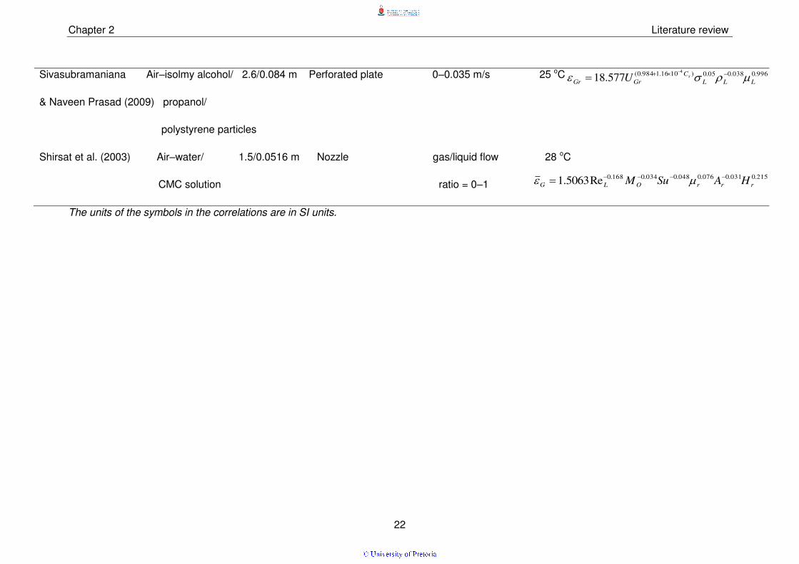
22
Sivasubramaniana Air–isolmy alcohol/ 2.6/0.084 m Perforated plate 0–0.035 m/s 25 oC
& Naveen Prasad (2009) propanol/
polystyrene particles
Shirsat et al. (2003) Air–water/ 1.5/0.0516 m Nozzle gas/liquid flow 28 oC
CMC solution ratio = 0–1
The units of the symbols in the correlations are in SI units.
996.0038.005.0)1016.1984.0( 4
577.18 LLL
C
GrGrsU
215.0031.0076.0048.0034.0168.0Re5063.1 rrrOLG HASuM

Chapter 2 Literature review
23
2.2.2 Measuring equipment and techniques
Many measuring techniques for gas holdup have been reported in the literature. This study
will only review a few of them.
2.2.2.1 Overall gas holdup
Overall gas holdup can be measured by the level expansion or pressure difference methods.
Zhang, Zhao & Zhang (2003) and Fransolet, Crine, L’Homme et al. (2001) compared the two
measuring techniques. Zhang et al. (2003) reported a close agreement between the two
techniques with a maximum percentage error of ±10%, as shown in Figure 2.5.
Figure 2.5: Comparison of the overall gas holdup measured by the pressure drop and the bed expansion method (Zhang et al., 2003)
Fransolet et al. (2001) reported that the two techniques agree with each other at low
superficial gas velocities but that a significant difference is observed at high superficial gas
velocities, as shown in Figure 2.6. They explained that this deviation can be attributed to the
fact that the volume of a column over which the gas holdup is determined is greater in the
level expansion method than it is in the pressure difference method.

Chapter 2 Literature review
24
Figure 2.6: Gas holdup as a function of superficial gas velocity obtained by using the level expansion and pressure difference methods (Fransolet et al., 2001)
2.2.2.2 Level expansion method
This technique is used to measure the level of gas–liquid dispersion and gas-free liquid for
calculating the gas holdup. Different techniques can be employed for measuring the liquid
level, such as visual observation, bubbler tube, floater/displacers, capacitance technique,
etc.
Visual observation: This is a simple technique in which the liquid level is measured
by a ruler or by a scale attached to the column wall. It can be applied only for
transparent columns. Orvalho, Ruzicka & Drahos (2009) reported the measurement
of the liquid level using a ruler. They explained that this technique will give a better
approximation in the homogeneous flow regime in which the liquid surface is well
defined, steady and horizontal. In the heterogeneous flow regime, the liquid surface
oscillates and the liquid level has to be measured by taking the mean of the lowest
and highest liquid surface positions. The measurements done by the authors were
taken from 10–20 oscillations, depending on the complexity of the motion. These
oscillations develop gradually and their amplitude increases with the gas flowrate
beyond the critical point. As the oscillation became intense, it became difficult to
measure the level with the ruler.

Chapter 2 Literature review
25
Bubbler tube: This is an inexpensive, simple and well-known technique. It does not
have temperature restrictions and it is mostly employed in corrosive and slurry-type
applications (Omega, 2001). It uses a dip tube installed with an open end. The
system consists of a tube, a gas supply, a pressure transmitter and a differential
pressure regulator. The regulator produces the constant gas flow required to prevent
calibration changes (Bahner, 2013). When a gas, usually air or an inert gas, is
flowing through the tube; bubbles escape from the open end. The air pressure in the
tube corresponds to the hydraulic head of the liquid at the outlet of the dip tube. The
air pressure in the bubble tube varies proportionally with the change in head
pressure. This technique is affected by changes in gas flowrate and liquid density.
The dip tube must be located far from the column bottom to prevent blockage of the
tube opening by slurry particles. The dip tube should have a reasonably large
diameter so that the pressure drop of gas flowing through the tube is negligible and
prevents the clogging of the dip tube if the gas is not filtered (Omega, 2001).
Floater and displacers: According to Archimedes Principle, the buoyancy force
acting on an object is equal to the weight of the fluid displaced (Omega, 2001). As
the level changes around the displacer float, which has a constant diameter and is
stationary, the buoyancy force varies in proportion to the level and can be detected
to give an indication of level (Omega, 2001).
Other level-measuring techniques are given in Table 2.2 (Omega, 2001). Many of these
cannot be applied to molten salt bubble columns due to high operating temperatures
and aggressive corrosion by molten salt in these systems.

Chapter 2 Literature review
26
Table 2.3: Level measuring techniques (Omega, 2001)
Type
M
axim
um
tem
pera
ture
(oF
)
Ac
cu
racy
Applications
Lim
itati
on
s
Liquids Solids
Cle
an
Vis
co
us
Slu
rry/s
lud
ge
Inte
rfa
ce
Fo
am
Po
wd
er
Ch
un
ky
Sti
cky
Capacitance 2000 1–2%
FS G F–G F G–L P F F P
Interface between conductive layers and
detection of foam is a problem.
Conductivity
switch 1800 1/8 in. F P F L L L L L
Can detect interface only between
conductive and non-conductive liquids.
Field effect design for solids.
Diaphragm 350 0.5%
FS G F–G F F F P Switches only for solid service.
Differential
pressure 1200
0.1%
AS E G–E G P
Only extended diaphragm seals or
repeaters can eliminate plugging. Purging
and sealing legs are also used.
Laser UL 0.5 in. L G G F F F F Limited to cloudy liquids or bright solids in
tanks with transparent vapour spaces.

Chapter 2 Literature review
27
Microwave
switches 400 0.5 in. G G F G G G F Thick coating is a limitation.
Optical
switches 260 0.25 in. G F E F–G F F P F
Refraction type for clean liquids only,
reflection type requires clean vapour
space.
Radar 450 0.12 in. G G F P P F P Interference from coating, agitator blades,
spray, or excessive turbulence.
Radiation UL 0.25 in. G E E G F G E E Requires nuclear regulator commission
licence.
Resistance
tape 225 0.5 in. G G G
Limited to liquids under near-atmospheric
pressure and temperature conditions.
Rotating
paddle
switch
500 1 in. G F P Limited to detection of dry, non-corrosive,
low-pressure solids.
Slip tube 200 0.5 in. F P P An unsafe manual device.
Tape-type
level
sensors
300 0.1 in. E F P G G F F
Only the inductively coupled float is suited
for interface measurement. Float hang-up
is a potential problem with most designs.

Chapter 2 Literature review
28
Thermal 850 0.5 in. G F F P F Foam and interface detection is limited by
the thermal conductive involved.
Ultrasonic 300 1%FS F–G G G F–G F F F G
Presence of dust, foam, dew in vapour
space; sloping or fluffy process material
interferes with performance.
Vibrating
switches 300 0.2 in. F G G F F G G
Excessive material build-up can prevent
operation.
AS = in % of actual span, E = Excellent, FS = in % of full scale, F = Fair, G = Good, L = Limited, P = Poor and UL = unlimited.

Chapter 2 Literature review
29
2.2.4 Effect of operating parameters on gas holdup
Gas holdup depends on the rising velocities of the bubbles. High gas holdup is attained for
low bubble rise velocities due to high bubble residence time. On the other hand, bubble rise
velocity is dependent on bubble sizes. Also, gas holdup is affected by the number of bubbles
in the column at a given superficial gas velocity.
2.2.4.1 Superficial gas velocity
Li & Prakash (2000) reported that gas holdup due to both small and large bubbles increases
with superficial gas velocity. Gas holdup due to large bubbles was found to be lower than
gas holdup due to small bubbles since large bubbles rise faster than small bubbles. The
difference between the two gas holdups was found to decrease as the superficial gas
velocity increases due to increased bubble coalescence.
Kumar et al. (1997) reported the effect of superficial gas velocity on the radial variation of
gas holdup. They found an increase in local gas holdup with superficial gas velocity for all
column radii, excluding the region close to the column wall. Gas holdup increased
insignificantly for lower gas velocities, showing a flatter profile, which confirms a bubbly flow
regime at the experimental conditions used. At higher gas velocities the gas holdup profile
became parabolic.
2.2.4.2 Operating temperature
Malayeri, Muller–Steinhagen & Smith (2003) also reported the effect of temperature on gas
holdup. They explained that an increase in temperature will result in the lowering of surface
tension and liquid viscosity, and an increase in vapour pressure. These combined effects will
result in an increase in the drainage and evaporation of the liquid film between the bubbles
and will thus enhance bubble coalescence. The authors also observed that a variation in gas
holdup becomes more significant near the boiling point.
Bukur, Petrovic & Daly (1987) reported the effect of temperature on gas holdup using
Fischer–Tropsch-derived paraffinic wax as a liquid medium. Studies were done in a
temperature range of 150–280 oC, where foamy and turbulent regimes were observed for
the superficial gas velocities used. In the foamy regime, gas holdup increased with
temperature, except for the gas holdups measured at 250 oC and 265 oC. In the turbulent
bubbling regime, the effect of temperature on gas holdup was very small for the temperature
range of 160–280 oC.

Chapter 2 Literature review
30
2.3 Axial dispersion coefficient
The modelling of bubble column reactors is often carried out assuming ideal plug flow
patterns for both the gas and liquid phases. However, such ideal fluid flow does not exist in
bubble columns and plug flow assumptions can result in deviations of design calculations
from reality (Nikolic, Nikolic, Veljkovic et al., 2004). However, in the homogeneous regime,
plug flow is normally assumed since the deviation from reality is minimal.
This non-ideal behaviour of fluid flow decreases the reactant conversion and affects the
selectivity. The study of non-ideal flow is therefore of particular importance for the design
and scale-up of bubble columns reactors and therefore it cannot be ignored (Nikolic et al.,
2004). Neglecting non-ideal flow can lead to detrimental errors when modelling, designing
and optimising bubble columns.
Two opposite magnitudes of axial dispersion may be desired when designing bubble
columns depending on the application. Most frequently, it is desired to have as low an axial
dispersion as possible to maintain the highest concentration driving force throughout the
column and attain higher reactant conversion (Dhanasekaran & Karunanithiy, 2010).
However, for the aerobic biological reactions operated in a semi-batch mode, it is desired to
attain a high axial dispersion as possible to ensure homogeneity in the fermentation broths.
The liquid backmixing is a result of various mechanisms, namely liquid circulations due to
non-uniform radial gas holdup, turbulent diffusion due to the eddies generated by rising
bubbles and molecular diffusion (Degaleesan & Dudukovik, 1998). Non-ideal flow of gases is
frequently encountered with wide bubble size distribution where gas bubbles travel with
different velocities. The rising bubbles carry the liquid upwards and the liquid has to return
downwards near the walls of the column, causing circulation patterns (Lakota, Jazbec &
Levec, 2001). Backmixing of the phases is therefore dependent on the magnitude of liquid
circulations.
2.3.1 Circulation patterns
Circulation cells occur in the heterogeneous flow regime. This is a high-interaction flow
regime which is characterised by circulation cells and polydispersed bubbles. In this flow
regime, gas holdup is non-uniformly distributed in the radial direction, as shown in
Figure 2.7. The radial variation of gas holdup results in a variation of gravitational pressure in
the radial direction, which increases from the column centre towards the column wall (Joshi
et al., 2002). As a result, liquid circulation will develop because of gravitational pressure

Chapter 2 Literature review
31
variations. In a circulation cell, the liquid flows in the upwards direction in the column centre
and downwards near the column wall. The liquid flow is zero at 0r before flowing down near
the wall. 0r is the radius of the column in which the liquid velocity is zero.
Figure 2.7: Schematic diagram of gas holdup and liquid velocity profile
One of the causes of backmixing of the phases is liquid circulation. The rising bubbles in a
bubble column carry the liquid in their wakes and in between them in the case of higher gas
loading (Groen, Oldeman, Mudde et al., 1996). The liquid carried by bubbles has to flow
down and thus results in the liquid circulation.

Chapter 2 Literature review
32
Figure 2.8: Liquid circulation patterns in bubble columns
In the circulation loop of the reactor, the liquid rises through the centre and flows downwards
near the column walls, as shown in Figure 2.8. Most of the gas bubbles rise up the column
centre and leave the reactor at the top surface. However, smaller gas bubbles will circulate
along with the liquid since they do not have enough buoyancy to disengage and leave the
column (Gupta, Ong, Al-Dahhan et al., 2001). The circulation mechanism is also facilitated
by bubble–bubble interactions, bubble wakes and shear-induced turbulence. Phase
circulation is therefore the main course of backmixing.
R R0

Chapter 3 Experimental setup and procedure
33
CHAPTER 3: EXPERIMENTAL SETUP AND PROCEDURE
3.1 Experimental setup
A schematic diagram and a photograph of the experimental setup used are shown in
Figures 3.1 and 3.2 respectively (See Appendix 10 for a photograph of the insulated
experimental setup). The experimental setup was designed to be operated with molten
lithium chloride (LiCl) and potassium chloride (KCl) eutectic at 450 oC. Before the column
was loaded with the salt, it was necessary to test its performance with liquids that are easy
to handle. Tap water and heat transfer oil 32 were used for this purpose. Heat transfer oil
was used to study the behaviour of the experimental setup as the temperature is ramped up.
Figure 3.1: Schematic diagram of the experimental setup

Chapter 3 Experimental setup and procedure
34
Figure 3.2: Photograph of the experimental setup
Experiments were carried out on the bubble column operated with water at 40 oC, heat
transfer oil at 75, 103 and 170 oC, and molten LiCl–KCl eutectic at 450 oC. The physical
properties of the liquids are given in Table 3.1. Argon gas was bubbled through the column
via the perforated plate gas distributor. The experiments were operated batchwise with
regard to the liquids and continuously with regard to argon. Heat was induced into the
column with the aid of three heating tapes. The liquid level was measured with a short and a
long bubbler tube. The height difference between the tip of the two bubbler tubes and the
gas distributor was fixed to 1.306 and 1.118 m for the short and long bubbler tubes
respectively.
Extraction
system
Copper pipe
Rotameters
Heating
tapes
Switches
and
voltmeters
Voltage
stabiliser
Voltage
regulator
Insulators
Copper cooling coil
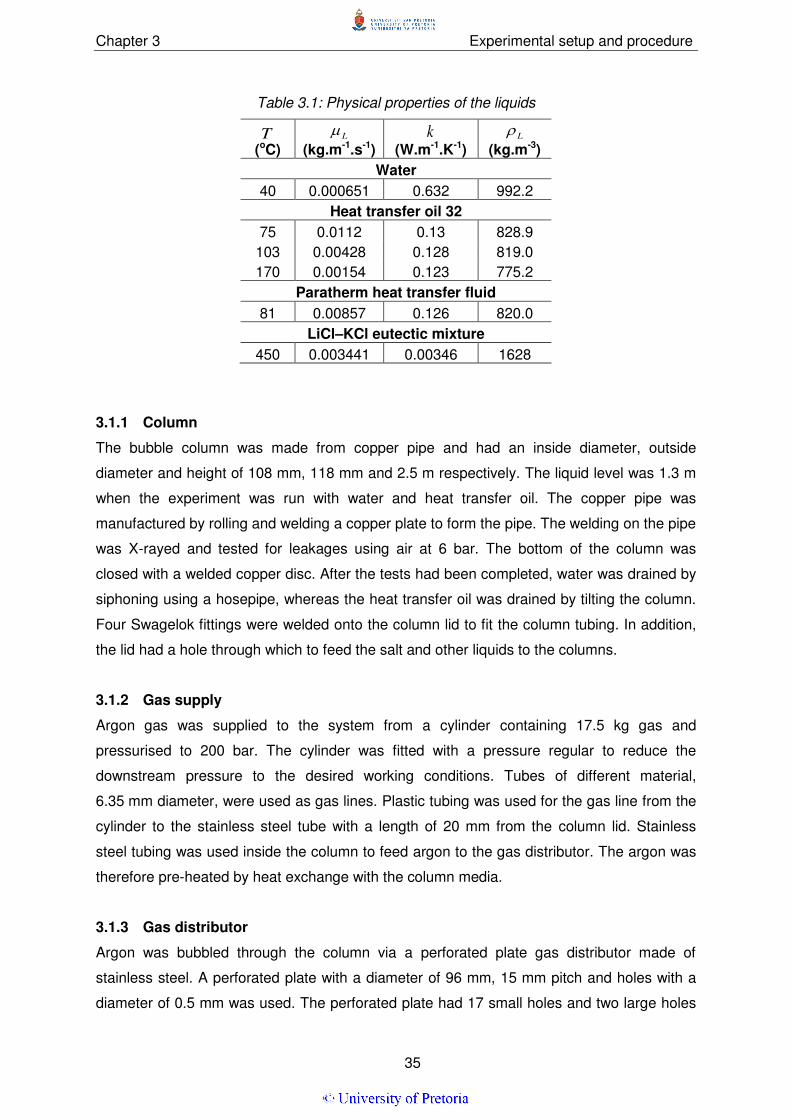
Chapter 3 Experimental setup and procedure
35
Table 3.1: Physical properties of the liquids
T (oC)
L
(kg.m-1.s-1)
k (W.m-1.K-1)
L
(kg.m-3)
Water
40 0.000651 0.632 992.2
Heat transfer oil 32
75 0.0112 0.13 828.9
103 0.00428 0.128 819.0
170 0.00154 0.123 775.2
Paratherm heat transfer fluid
81 0.00857 0.126 820.0
LiCl–KCl eutectic mixture
450 0.003441 0.00346 1628
3.1.1 Column
The bubble column was made from copper pipe and had an inside diameter, outside
diameter and height of 108 mm, 118 mm and 2.5 m respectively. The liquid level was 1.3 m
when the experiment was run with water and heat transfer oil. The copper pipe was
manufactured by rolling and welding a copper plate to form the pipe. The welding on the pipe
was X-rayed and tested for leakages using air at 6 bar. The bottom of the column was
closed with a welded copper disc. After the tests had been completed, water was drained by
siphoning using a hosepipe, whereas the heat transfer oil was drained by tilting the column.
Four Swagelok fittings were welded onto the column lid to fit the column tubing. In addition,
the lid had a hole through which to feed the salt and other liquids to the columns.
3.1.2 Gas supply
Argon gas was supplied to the system from a cylinder containing 17.5 kg gas and
pressurised to 200 bar. The cylinder was fitted with a pressure regular to reduce the
downstream pressure to the desired working conditions. Tubes of different material,
6.35 mm diameter, were used as gas lines. Plastic tubing was used for the gas line from the
cylinder to the stainless steel tube with a length of 20 mm from the column lid. Stainless
steel tubing was used inside the column to feed argon to the gas distributor. The argon was
therefore pre-heated by heat exchange with the column media.
3.1.3 Gas distributor
Argon was bubbled through the column via a perforated plate gas distributor made of
stainless steel. A perforated plate with a diameter of 96 mm, 15 mm pitch and holes with a
diameter of 0.5 mm was used. The perforated plate had 17 small holes and two large holes

Chapter 3 Experimental setup and procedure
36
of 6.5 mm diameter, as shown in Figure 3.3 (Appendix 8 shows the design of the
perforations). Two argon inlet tubes were fitted in the 6.5 mm holes.
Figure 3.3: Perforated plate showing the arrangement of the orifices
As shown in Figure 3.4, the gas distributor was made from the perforated plate welded to the
gas chamber below it. The gas distributor had a V-shaped gap to enable it to pass the
thermowells inside the column when it was inserted through the top of the column during
installation.
Figure 3.4: Gas distributor fitted with ¼ in. stainless steel tubing
3.1.4 Heat transfer section
Three heating tapes, each with dimensions of 3 000 mm × 44 mm and a power rating of
1 570 W, were used as the heat source. Each heating tape was wrapped around the copper
pipe to form a heating zone of 350 mm in length. Thus the total length of the heating section
was 1 050 mm. The top and bottom heaters were used as guard heaters to minimise the
Perforation Tubing
Gas chamber
Perforated
plate

Chapter 3 Experimental setup and procedure
37
axial heat conduction at the ends of the heater in the middle. The heat transfer flux from the
middle heater could be measured accurately and hence by using the power input of the
middle heater, the heat transfer coefficient could be calculated accurately. The heating tapes
were insulated with ceramic fibre insulation which was vacuum-formed and moulded to a
thickness of 75 mm and i.d. of 135 mm. Temperature differences were measured at five
different points along the column using pairs of type K thermocouples with 2 mm diameter
sheaths.
Each pair consisted of a thermocouple that measures the wall temperature and another that
measures the liquid temperature. The spacing between the five pairs of thermocouples was
170 mm. Liquid temperatures were measured by inserting thermocouples through the
thermowells which are welded to the copper pipe. The thermowells were made from ¼ in.
stainless steel tubing welded to a copper rod and the total length of each thermowell was
30 mm. In order to measure the wall temperature accurately, the thermocouples were silver-
soldered on the outside wall of the copper pipe, as shown in Figure 3.5.
Figure 3.5: Thermocouples soldered to the wall of the copper pipe
The tips of the thermocouples in a pair were placed at the same axial position. This was
done to account for the fact that a temperature gradient formed along the height of the
column. The thermocouples were calibrated using a water bath with a uniform temperature
and the average error in the calibration results was less than 0.35 oC (see Appendix 7).
The power of the heaters was controlled by the AC voltage controllers. A voltage stabiliser
was also installed to supply the voltage controllers with a stable voltage. To balance the
system, heat was removed by cooling water flowing through the copper tube on the inside of
Soldered
thermocouples
Chapter 3 Experimental setup and procedure
38
the column. The removal of heat by the cooling water also increased the temperature
difference and therefore improved the accuracy of the measurements. The coiled copper
tube was positioned above the heating section so that it did not significantly change the
hydrodynamics in the heating section. Above the heating section, the column was also
insulated to maximise the absorption of heat by the cooling water.
The rate of heat transfer was obtained by measuring the voltage across an electric current
flowing through the heating tapes. A multimeter was used to measure the voltage and a
clamp current meter was used to measure the current. The measurements of the rate of heat
transfer were confirmed by calculating the energy balance over the cooling water coil.
3.1.5 Modified experimental setup
Due to the column failing when it was operated with molten salt, it had to be modified.
Figure 3.6 shows the modified experimental setup that was also used to measure the heat
transfer coefficients. The column was modified by making the following changes:
The height of the column was reduced from 2.5 m to 1.4 m.
The liquid level was reduced from 1.3 m to 0.9 m.
Heating tapes were replaced with heating cables.
The liquid temperature was measured by long thermocouples inserted from the
column lid.
The thermowells were omitted.

Chapter 3 Experimental setup and procedure
39
Figure 3.6: Schematic diagram of the modified experimental setup
3.2 Experimental procedure
3.2.1 Heat transfer coefficient
The heat transfer coefficient was calculated from Equation 3.1:
)( BW TTA
Qh
[3.1]
where Q is the rate of heat transfer, A is the heat transfer area, WT is the wall temperature
and BT is the bulk liquid temperature. The rate of heat transfer is calculated from:

Chapter 3 Experimental setup and procedure
40
lossQPQ [3.2]
where,
L
TAkQ iloss
[3.3]
where P is the electrical power, lossQ is the heat loss from the heating tapes to the
surrounding environment, ik is the thermal conductivity of the insulation material, L is the
distance between the measured temperature difference and is the temperature
difference at L ( L = 45 mm was used).
3.2.1.1 Column operated with water
The experiments were conducted as follows:
The column was filled with water up to a level of 1.3 m.
The heaters were switched on to increase the temperature of the water.
The rotameter for the cooling water was turned on to remove heat from the column
and increase the temperature difference between the column wall and the liquid.
After the heaters had stabilised, the liquid temperature was controlled at 40 oC.
Rotameters were used to control the argon flowrate to superficial gas velocities in the
range of 0.006–0.05 m/s.
Measurements and readings were taken after the system had reached steady state.
Power and temperature readings were taken at each gas flowrate.
The experimental procedure was repeated four times on different days for each
superficial gas velocity.
3.2.1.2 Column operated with heat transfer oil
The experimental procedure for heat transfer oil at 75 oC and 103 oC was performed in a
similar way to that for water, except that at 170 oC the system was operated without cooling
water. The power of the heating tapes could not raise the oil temperature up to 170 oC while
heat was being removed using the cooling water. Also, at 170 oC when the column was
operated without cooling water, the temperature difference between the column wall and the
liquid was high enough to be measured accurately. The insulation above the heating section
was removed so that heat could be removed through the upper column wall. Furthermore,
for the experiments at 103 oC, the heating tapes were at maximum power for higher
superficial gas velocities and cooling water was used to control the liquid temperature.
iT

Chapter 3 Experimental setup and procedure
41
3.2.1.3 Column operated with molten salt mixture
The salt used was a eutectic mixture of LiCl and KCl. Approximately 18 kg of the salt
eutectic was weighed and melted. The masses of LiCl and KCl were 8 kg and 9.95 kg
respectively. This was achieved by initially melting 13.6 kg of the salt eutectic at 450 oC and
filling the heating zone with the salt in a molten state. The remaining 4.35 kg was then added
and quickly melted as it settled in the pool of molten salt. See Appendix 9 for a detailed
calculation of the amount of each salt in the eutectic mixture.
3.2.2 Gas holdup
Appendix 6 shows the derivation of the equations needed to calculate the gas holdup. The
procedure for measuring the gas holdup was the same for all the liquids used.
The argon flowrate was controlled with the aid of rotameters.
The argon flow was switched on and the flowrate varied to give a superficial gas
velocity in the range of 0.006 m/s to 0.05 m/s.
The flowrate in the bubbler tubes was kept at 2–3 l/h for all level measurements.
Bubbler tubes were used to measure the change in the liquid level due to an increase
in the superficial gas velocity.
Manometer readings were taken at each argon flowrate.
This procedure was done three times.
3.3 Experimental understanding
3.3 1 Impact of cooling water
The heat transfer area of the bubble column was very large. Therefore for the operating
temperatures of 40 oC, 75 oC and 103 oC a low heat was needed in order for the system to
reach steady state at the desired operating temperature. Heat loss from the column contents
to the surroundings was therefore very low and that could have reduced the temperature
difference between the column wall and the liquid to below 1 oC, which could be difficult to
measure accurately. More heat was therefore removed to increase the temperature
difference to a value that could be measured accurately. Heat was removed by using cooling
water flowing through a ¼ in. coiled copper tube. In order to keep the system at steady state
at the desired temperature, more heat was added to compensate the heat absorbed by the
cooling water. Additionally, the use of cooling water was useful in the verification of the
measurements of electrical power.

Chapter 3 Experimental setup and procedure
42
3.3.2 Comparison between stainless steel and copper bubble column
Since bubble columns have high values of heat transfer coefficients, a copper pipe was
considered for measuring the heat transfer coefficient because of its higher thermal
conductivity. This higher thermal conductivity ensures that the resistance to conductive heat
transfer is higher than the resistance to convective heat transfer, so that the radial and axial
temperatures in the pipe wall can be distributed faster and attain uniformity. For an
aggressive medium such as molten salt, stainless steel is a good material of construction.
However, the thermal conductivity of stainless steel is 25 W.m-2.K-1 which is very low
compared with the 300 W.m-2.K-1 of copper. As a result, the temperature might not be
uniform when a stainless steel pipe is used.
The temperature profile for a copper pipe as heated in the experimental column was
compared with that of a stainless steel pipe by modelling the two-dimensional heat
conduction in the pipe wall using the software package Abaqus Version 6.12. The modelling
was done on a pipe wall 8 mm thick and with a spacing of 20 mm between two heating
elements that are at the same temperature. The boundary conditions were as follows:
It was assumed that the two heating elements are at the same temperature of 72 oC.
Therefore the top and bottom boundary conditions were that the temperature is
72 oC.
On the inner side of the pipe, there is a gas-liquid dispersion with a heat transfer
coefficient of 2 000 W.m-2.K-1.
On the outer side of the pipe, there is natural convection by air with a heat transfer
coefficient of 10 W.m-2.K-1.
Figure 3.7 shows the calculated two-dimensional temperature profile in the wall of a
stainless steel pipe. The temperature was not uniform since there was a temperature
difference of about 5 oC between the maximum and minimum temperatures. It would
therefore be difficult to measure the temperature difference between the wall and the liquid
in the column accurately when using stainless steel. The average inner wall temperature
would not be estimated accurately due significant non-uniformity of the temperature in both
the axial and radial directions. It could also be difficult to position the thermocouple in the
column wall in such a way that it measures the inner wall temperature accurately. This is
because the distance between the bi-metallic coupling of the thermocouple and the tip of the
thermocouple sheath is not known, thus making it difficult to compensate for the heat
conduction through the column wall when estimating the inner wall temperature.

Chapter 3 Experimental setup and procedure
43
Figure 3.7: Temperature profile between spacing of heating elements for a stainless steel pipe
Figure 3.8 shows the predicted two-dimensional temperature profile of the wall of a copper
pipe. As shown in the figure, the temperature is uniform in both the axial and radial
directions, with a temperature difference of about 0.8 oC between the maximum and
minimum temperatures. The high thermal conductivity of a copper pipe ensures a nearly
uniform temperature in the wall. Such temperature uniformity is important due to the fact that
the thermocouple at the wall could be positioned almost anywhere in the axial or radial
directions and still give a good measurement of the inner wall temperature of the pipe. The
temperature difference would therefore be measured accurately when a copper pipe was
used and that was the main reason for choosing a copper pipe for the experiments.

Chapter 3 Experimental setup and procedure
44
Figure 3.8: Temperature profile between spacing of heating elements for a copper pipe
3.3.3 Modelling of the temperature profile in the thermowell
Thermowells were welded to the bubble column wall. Figure 3.9 shows a photograph of one
of the thermowells that were used to measure the liquid temperature. The copper part of the
thermowell was threaded to allow it to be fitted to the threaded hole in the column wall. The
fitted thermowell was then welded onto the column wall for proper sealing. Stainless steel
extensions were welded onto the copper thermowells. Stainless steel was included in the
thermowell because there is a large temperature gradient on the heated stainless steel
which ensures a good representation of the liquid temperature to be measured. When the
column wall is being heated, the thermowell conducts heat and that poses challenges with
regard to isolating the heat conducted by the thermowell and the sensitivity of the
thermocouple that measures the liquid temperature. The thermowell should therefore be a
poor conductor of heat in order for the thermocouple to measure only the liquid temperature
without sensing any heat from the wall.

Chapter 3 Experimental setup and procedure
45
Figure 3.9: Thermowell used for temperature measurements
The purpose of this modelling was to determine whether the temperature measured at the tip
of the well would be representative of the liquid surrounding the tip, thus confirming the
reason for the inclusion of stainless steel in the thermowell for measuring a liquid
temperature correctly. Assuming that there is no temperature gradient in the radial direction
of the wall of the thermowell, the energy balance for a small element of x is given by:
)(2 Bxxx TTxhqq [3.4]
Rearranging Equation 3.4 and dividing the equation by x gives:
x
TTxrh
x
x
Bxxx
2
0
lim [3.5]
BTTrhdx
dq 2 [3.6]
BTTrhdx
dTkA
dx
d
2 [3.7]
Copper
Stainless steel
30 mm

Chapter 3 Experimental setup and procedure
46
Differentiating and rearranging Equation 3.7 gives:
BTTkA
rh
dx
Td
22
2
[3.8]
Let yTT B and 22b
kA
rh
Differentiating yTT B twice gives:
2
2
2
2
dx
yd
dx
Td [3.9]
Substituting Equation 3.9, y and b into Equation 3.8 gives:
02
2
2
ybdx
yd [3.10]
The general solution to Equation 3.10 is given by:
bxbx
eCeCy 21 [3.11]
Substituting Equation 3.11 into yTT B gives:
bxbx
B eCeCTT 21 [3.12]
Differentiating Equation 3.12 gives:
bxbxeCeCb
dx
dT21 [3.13]
The boundary condition at beginning of the thermowell is:
WTT at 0x

Chapter 3 Experimental setup and procedure
47
Substituting the above boundary condition into Equation 3.12 therefore gives:
21 CCTT BW [3.14
The boundary condition of the tip of the thermowell is:
)( Bt TThdx
dTk
at Lx
Substituting the above boundary conditions into Equation 3.13 gives:
bxbx
B
t eCeCbTTk
h21)( [3.15]
Substituting Equation 3.12 into Equation 3.15 yields:
bLbLtbLbLeCeC
k
heCeCb 2121
[3.16]
Substituting Equation 3.14 into Equation 3.16 and making 1C the subject of the equation
gives:
bLbLtbLbL
tbL
BW
eekb
hee
kb
heTT
C
1
1 [3.17]
For L = 0.03 m, BT = 40 oC,
WT = 45 oC, steelk = 25 W.m-2.K-1,
copperk = 300 W.m-2.K-1,
th = 3 000 W.m-2.K-1, r = 3.175 mm, Equation 3.12 is plotted in Figure 3.10. The
temperature gradients for copper and stainless steel thermowells are plotted and compared.
As shown in Figure 3.10, the stainless steel thermowell gives a better representation of the
liquid temperature in a bubble column due to the large temperature difference between the
beginning and the tip of the thermowell. It was concluded that a stainless steel tip of 12 mm
would be adequate.

Chapter 3 Experimental setup and procedure
48
Figure 3.10: Temperature profile for stainless steel and copper thermowells
40
42
44
46
0 0.004 0.008 0.012 0.016 0.02 0.024 0.028 0.032
T(o
C)
x (m)
Copper Steel

Chapter 4 Results and discussion
49
CHAPTER 4: RESULTS AND DISCUSSION
4.1 Heat transfer coefficient
4.1.1 Column operated with water
Table 4.1 shows the values of heat input, which is the rate of heat generated by the heaters
and transferred to the column; and heat output, which is calculated from the energy balance
of the cooling water.
Table 4.1: Comparison of heat input and heat output
When the system reaches steady state, heat input must equal to heat output. It was found
that the values of heat input and heat output are close to one another, with some small
errors that were regarded as acceptable. Therefore, the rate of heat transfer was measured
accurately. Table 4.2 shows the values of the temperature difference at different axial
positions of the copper pipe. The second difference pair, 2V , was omitted from the
calculations of average temperature difference because, according to Dixon’s test of outliers,
there is more that 95% confidence that it is an outlier (Grubbs, 1969).
Table 4.2: Temperature difference measured at different axial positions of the heating zone
for = 0.031 m/s
It was expected that the temperature difference between the wall and the liquid would be
uniform as a result of the high thermal conductivity of the copper metal. The values of the
Gu
[m/s]
Total
power
[W]
Heat
loss
[W]
Heat
input
[W]
Heat
output
[W]
%
error
0.006 1 543.8 52.1 1 491.7 1 510.3 1.3
0.015 2 031.0 69.8 1 961.2 1 936.5 1.3
0.023 2 386.9 79.5 2 307.4 2 248.1 2.6
0.031 2 795.0 91.8 2 703.2 2 546.1 5.8
0.039 3 222.0 102.4 3 119.5 2 897.8 7.1
0.046 3 665.9 118.5 3 547.4 3 367.3 5.1
1V
[mV]
2V
[mV]
3V
[mV]
4V
[mV]
5V
[mV]
averageV [mV]
averageT [oC] s
0.085 0.133 0.080 0.085 0.101 0.097
2.1 3.3 2.0 2.1 2.5
2.2 0.192
Gu
VT

Chapter 4 Results and discussion
50
temperature difference are close to one another with the standard deviation, s , of 0.192 and
this confirms the uniformity of the wall temperature.
Figure 4.1: Different runs for measuring the heat transfer coefficient
The experiments for measuring the heat transfer coefficient were repeated several times on
different days to check the repeatability of the experimental setup. The results of different
runs in Figure 4.1 show that the experiment was repeatable, with an experimental error
ranging from 0.5 to 4% (Appendix 1 and 4 shows the values of experimental error and how
was it calculated, respectively). The heat transfer coefficient increases with superficial gas
velocity. As the superficial gas velocity increases, the number of bubbles increases and this
reduces the surface film thickness. The heat transfer coefficient will thus be lowered as a
result of the reduced surface film thickness.
The measured heat transfer coefficients were compared with those in the literature, as
shown in Figure 4.2. Recent developments regarding work on the wall heat transfer
coefficient are very rare and the comparison was therefore made with the old research work.
1500
1700
1900
2100
2300
2500
2700
2900
0 0.01 0.02 0.03 0.04 0.05 0.06
h (
W.m
-2.K
-1)
UG (m/s)
1st run 2nd run 3rd run 4th run

Chapter 4 Results and discussion
51
Figure 4.2: Comparison of experimental heat transfer coefficient with the literature for measurements in water medium
The experimental values for the heat transfer coefficient are in good agreement with those of
Kast (1963), and in somewhat less good agreement with those of Deckwer (1980a), Hart
(1976) and Fair et al. (1962). However, the results of Kast (1963) might have deviated from
the other literature results because of uncertainties in the way the correlation of Kast (1963)
is written. In Table 2.1 (Chapter 2) the gas viscosity is included in the correlation of Kast
(1963) which is peculiar.
The experimental results for the heat transfer coefficients that were measured in the
modified experimental setup in Figure 3.6 (Chapter 3) are shown in Figure 4.3. These results
show better agreement with the literature compared with those in Figure 4.2. The difference
in the results obtained for these two systems could be attributed to the difference in the way
the liquid temperature was measured in the two systems. In the modified setup, the
thermocouples that were inserted from the column lid were closer to the inner surface of the
bubble column. In Figure 3.2 (Chapter 3) the liquid temperature was measured by using
thermowells that were 30 mm long and they measured the liquid temperature near the
column centre. Therefore, the thermowells contributed to a slightly larger temperature
difference compared with the thermocouples in the modified system.
0
1,000
2,000
3,000
4,000
5,000
6,000
0.00 0.01 0.02 0.03 0.04 0.05 0.06
h (
W.m
-2.K
-1)
UG (m/s)
Experimental Deckwer (1980) Hart (1976)
Kast (1963) Fair et al. (1962)

Chapter 4 Results and discussion
1. Results for the modified setup are shown only in Figure 4.3, all the other results are for the setup in
Figure 3.2.
52
Figure 4.3: Comparison of experimental heat transfer coefficient with the literature for measurements in water medium in the modified experimental setup1
It is normally assumed that there is no radial temperature profile between the column centre
and a liquid–film interface. However, there is a temperature gradient from the column centre
towards the wall and the assumption of no temperature gradient can result in disparities
between the measurements of the temperature between the wall and the fluid. In Appendix 5
it is shown that the temperature difference between the column centre and a liquid–film
interface could be 0.4 oC or more. For the temperature differences that were measured in
the system shown in Figure 3.2 (Chapter 3), as shown in Table 4.2 above, the radial
temperature profile could have affected the measurements by about 20%.
4.1.2 Column operated with heat transfer oil
Heat transfer coefficients for the argon–heat transfer oil system are shown in Figure 4.4.
Similar to the argon–water system, the heat transfer coefficient increases with superficial gas
velocity due to an increased number of bubbles and turbulence in the system. For the
operating temperatures of 75 oC and 103 oC, the heat transfer coefficient flattened out above
a superficial gas velocity of 0.035 m/s. At the operating temperature of 170 oC, the heat
0
1000
2000
3000
4000
5000
6000
0.000 0.010 0.020 0.030 0.040 0.050 0.060
h (
W.m
-2.K
-1)
UG (m/s)
Experimental Deckwer (1980) Hart (1976)
Kast (1963) Fair et al. (1962)

Chapter 4 Results and discussion
53
transfer coefficient increased significantly. At = 0.05 m/s, the heat transfer coefficient of
the second graph was lower than that at = 0.045 m/s. At
= 0.05 m/s, the operating
temperature was controlled to 98 oC instead of 103 oC because the heating tapes were
already at their maximum power and the cooling water could not control the temperature
effectively. Since the measurements at 103 oC were not done at constant temperature, the
slight differences in physical properties affected the results.
Figure 4.4: Heat transfer coefficient at different temperatures
The heat transfer coefficients for the argon–heat transfer oil system are lower than those
obtained for the argon–water system. The viscosity of heat transfer oil is higher than that of
water. The bubble sizes increase with an increase in liquid viscosity. Large bubbles rise at
the core of the bubble column with little turbulence at the column wall. Therefore, the wall
heat transfer coefficient of the oil compare to that of water is significantly affected by the
liquid thermal conductivity than the viscosity. The high heat transfer coefficient of the argon–
water system is therefore attributed to the higher thermal conductivity of water compared to
heat transfer oil. On the other hand, as shown in Figure 4.4, the heat transfer coefficient
increases with an increase in temperature.
There are no data available in the literature for heat transfer coefficients in a bubble column
operated with heat transfer oil 32. The experimental values at 75 oC were compared with
those of another heat transfer fluid. Yang, Luo, Lau et al. (2000) measured the heat transfer
Gu
Gu Gu
0
100
200
300
400
500
600
700
800
900
1,000
0.00 0.01 0.02 0.03 0.04 0.05 0.06
h (
W.m
-2. K
-1)
UG (m/s)
75 degree C 103 degree C 170 degree C

Chapter 4 Results and discussion
54
coefficient in a bubble column operated with air and Paratherm NF heat transfer fluid at
81 oC and 4.2 MPa.
Differences between the experimental results and the literature are attributed to different
physical properties of the two oils. It can also be observed in Figure 4.5 that the heat transfer
coefficient for the heat transfer fluid is lower than that when the system is operated with
water; this confirms that an increase in liquid viscosity decreases the heat transfer
coefficient.
Figure 4.5: Comparison of heat transfer coefficients with the literature for measurements in heat transfer oil medium
4.1.3 Column operated with molten salt mixture
The photographs in Figure 4.6 show the mechanical failure of the experimental setup after it
had been operated with molten salt. The weld of the thermowells failed and caused the salt
to leak. The molten salt was then exposed to oxygen and caused an aggressive corrosion of
the pipe within hours. All three heating tapes were also damaged beyond repair by the
molten salt.
0
100
200
300
400
500
600
700
0 0.01 0.02 0.03 0.04 0.05 0.06 0.07 0.08 0.09 0.1
h (
W/m
2K
)
UG (m/s)
Yang et al. (2000) Experimental

Chapter 4 Results and discussion
55
Figure 4.6: Copper pipe damaged by leakage of molten salt
After the salt had leaked through the welds of the thermowells and the column, it was
decided to cut the 2.5 m copper pipe into a 1.4 m length and heat it with ceramic band
heaters. A ceramic band heater with three heating zones was used because the heating
cables shown in Figure 3.6 (Chapter 3) were damaged and they could not be used again.
The new test rig did not have any thermowells, although there were some other welds since
the pipe was a welded copper plate. Figure 4.7 show the experimental setup before the salt
was loaded.
Figure 4.7: Experimental setup before salt leakage (new test rig)

Chapter 4 Results and discussion
56
After the column in the new test rig had been operated with molten salt, it was also found to
have leaked at the welds. Figure 4.8 shows the experimental setup after the salt had leaked
out of the column.
Figure 4.8: Experimental setup after salt leakage
4.2 Gas holdup
4.2.1 Column operated with water
As shown in Figure 4.9, gas holdup increases with superficial gas velocity (experimental
data for gas holdup can be obtained in Appendix 2). As the superficial gas velocity
increases, the number of bubbles increases, thus increasing the gas holdup. The
experimental results were in good agreement with the literature.

Chapter 4 Results and discussion
57
Figure 4.9: Comparison of experimental results for gas holdup with the literature
4.2.2 Column operated with heat transfer oil
The gas holdup for the heat transfer oil also increased with superficial gas velocity and
temperature, and was greater than that of the argon–water system. This can be attributed to
the higher operating temperature.
Figure 4.10: Experimental gas holdup at heat transfer oil
0
0.05
0.1
0.15
0.2
0.25
0 0.01 0.02 0.03 0.04 0.05 0.06
Ga
s h
old
up
(-)
UG (m/s)
Experimental Jawad et al. (2009)
0.00
0.05
0.10
0.15
0.20
0.25
0.30
0.35
0.000 0.010 0.020 0.030 0.040 0.050
Ga
s h
old
up
(-)
UG (m/s)
170 degree C 75 degree C

Chapter 4 Results and discussion
58
4.3 Mechanistic model for dispersion coefficients
4.3.1 Liquid flow model
Ueyama & Miyauchi (1970) applied a force balance equation to develop a theoretical model
for predicting a liquid velocity profile. Equation 4.1 is basically the sum of forces acting on
liquid in a bubble column.
gdZ
dPr
dr
d
rLG 1
1 [4.1]
where r is a radial coordinate, is the shear stress, P is the pressure and Z is the axial
coordinate.
The shear stress is given by:
dr
duLtM [4.2]
where is u the interstitial liquid velocity, M is the molecular viscosity (whose contribution is
due to the random movement of molecules) and t
is the turbulent kinematic viscosity
(whose contribution to momentum exchange is due to circulation cells). Integrating
Equation 4.1 between 0r and Rr gives:
gRdZ
dPLGw
1
2 [4.3]
where W is the shear stress at the wall. Substituting Equations 4.3 and 4.2 into
Equation 4.1 (neglecting M in the turbulent core), one obtains the modified basic equation
for axial liquid flow in the turbulent core:
gRdr
dur
dr
d
rGGw
l
t
21 [4.4]

Chapter 4 Results and discussion
59
Equation 4.4 can be solved by applying the following simplifying assumptions: (a) t is
constant throughout the turbulent core region of the column, and (b) the profile of the gas
holdup is approximated by Equation 4.5:
n
G
G
n
n
12
[4.5]
Boundary conditions:
0dr
du at 0r
Ueyama & Miyauchi (1979) used the universal velocity profile to model the laminar sublayer
at the wall, assuming that both the laminar sublayer and the buffer layer consist of only
liquid. The liquid velocity at the wall was found to be equal to:
LwWu /63.11 at Rr
The solution that satisfies the above boundary conditions is given by:
22
2
12
122
nGG
l
w
t
wnn
g
n
g
R
Ruu
[4.6]
Let
)2(
2
nn
gRN G
t
[4.7]
and
n
g
R
RP G
L
W
t 22
2
[4.8]
From the boundary condition at Rr , the shear stress at the wall is given by:

Chapter 4 Results and discussion
60
2
63.11
W
LW
u [4.9]
Substituting Equation 4.9 into Equation 4.8 yields:
n
g
R
uRP GW
t 2263.11 2
22
[4.10]
Substituting Equations 4.7 and 4.8 into Equation 4.6 gives:
22 11 n
W NPuu [4.11]
From Equation 4.5, let
n
nM G
2 [4.12]
Equation 4.5 then becomes:
n
G M 1 [4.13]
However, there are four unknowns in Equation 4.6, namely: an interstitial liquid velocity, the
liquid velocity at the wall, the shear stress at the wall and the turbulent kinematic viscosity.
These unknowns can be estimated by substituting Equation 4.6 or Equation 4.11 and
Equation 4.9 into a liquid mass balance expression inside the column, as given by:
0120
drru G
R
L [4.14]
Equation 4.14 implies that the sum of the liquid mass flowrates in the circulation patterns is
equal to zero for a semi-batch column.
In Equation 4.14, by substituting Rr , one obtains:

Chapter 4 Results and discussion
61
1
0
2 0)1(2 duR G [4.15]
Substituting Equations 4.11 and 4.13 into Equation 4.15 gives:
1
0
222 011112 dMNPuRnn
w [4.16]
Integrating Equation 4.16 yields:
222
422
422
22
222
422
422
22
nMuR
nNRPRuR
n
W
n
W
042422
24242
2
1
0
424222
42422
nnnNMR
nnPMR
nnnnn
[4.17]
Simplifying Equation 4.17 yields:
4
1
2
1
4
12
2
1
2
12
4
1
2
12
2
1 22222
nnPMR
nMuR
nNRPRuR WW
042
1
4
1
2
1
2
12 2
nnnNMR [4.18]
Substituting Equation 4.10 into Equation 4.18 gives:
2
1
2
12
4
1
2
12
2263.112
1 22
2
24
2
nMuR
nNR
n
g
R
uRuR W
GW
t
W
4
1
2
1
4
1
2263.112
2
24
nnn
g
R
uRM GW
t
042
1
4
1
2
1
2
12 2
nnnNMR [4.19]

Chapter 4 Results and discussion
62
Simplifying Equation 4.19 gives:
2
1
2
12
4
1
2
1
4
1
63.1163.114
1 22
2
23
2
23
nMuRuR
nn
uMRuRWW
t
WW
t
4
1
2
1
4
1
4
1
2
12
4
14
24
nnn
MR
nNR
n
gR
t
GG
t
042
1
4
1
2
1
2
12 2
nnnNMR [4.20]
Wu can be calculated by solving the quadratic formula provided that the values of tv , R , n ,
g and G are known. u will therefore be calculated for any radial position. The correlations
to calculate exponential factor, n , are not generally available. However, in the churn
turbulent flow regime, the exponential levels off to a value of approximately 2 as the superfial
gas velocity increases (Shaikh & Al-Dahhan, 2005).
4.3.2 Model for turbulent viscosity and dispersion coefficients
In this section, a mechanistic model for estimating the kinematic turbulent viscosity and
dispersion coefficient was developed. A similar approach to that of Ueyama & Miyauchi
(1979) was used in developing the model. The major difference is that, whereas Ueyama &
Michauchi (1979) determined the turbulent viscosities by fitting their model to liquid
velocities, this work describes a way of estimating kinematic turbulent viscosity using a
mechanistic model for the momentum exchange in bubble columns.
The turbulent viscosity is a function of the liquid flow patterns that cause momentum
exchange between circulation cells. For ordinary molecular viscosity, the mechanism of
momentum exchange is the random movement of molecules between different layers of flow
which exchange momentum. In the case of turbulent flow on a larger scale, liquid eddies
exchange momentum in a similar way to that of the molecules in viscous flow. In a bubble
column, it is assumed that the circulation cells cause exchange of momentum.
Analogous to the kinetic gas theory for molecular viscosity or to the Prandtl mixing length
theory for turbulent flow, the turbulent viscosity is defined as the product of the mass flux

Chapter 4 Results and discussion
63
across the surface of a differential control volume and a penetration depth which is the
distance that liquid in a circulation cell has to travel before it acquires the same momentum
as that of the liquid in its new environment.
Figure 4.11: Schematic diagram depicting the momentum exchange between circulation cells
Figure 4.11 shows the mechanism of momentum exchange in bubble columns. In order to
estimate the turbulent viscosity, the mass flux, G , across the curved surface where the liquid
velocity is zero is used. The turbulent viscosity is the product of this mass flux and the
distance that has to be travelled by a lump of fluid for it to change momentum, , as given
by:
Gt [4.21]
The kinematic turbulent viscosity will therefore be calculated from:
L
upwards
tZr
m
02
[4.22]

Chapter 4 Results and discussion
64
where upwardsm is the liquid mass flowrate in the upward direction in the circulation cell, 0r is
the radius of the column in which the liquid velocity is zero and Z is the height of the
circulation cell. The curved surface at 0r is used to calculate G since the liquid flowing
upwards with the flowrate upwardsm has to cross this curved surface area before flowing
down. Joshi & Sharma (1979) used an energy balance technique to show that the energy of
a recirculation cell is at a minimum when the height of the cell is equal to the diameter of the
column. However in this work, after comparing the model to data published in the literature
when assuming that the exponential factor � equals 2, the height of the circulation cells was
found to be approximately equal to 1.4 times the column diameter. The penetration depth is
expected to be dependent on the column radius because the column wall confines the
movement of the liquid and, therefore, the liquid is forced to change its momentum. The
circulation cells are often symmetrical about the column centre; therefore, it was assumed
that the penetration depth is approximately equal to half of the column radius.
The upwards mass flowrate is calculated from:
0
0
12
r
GLupwards drurm [4.23]
Substituting 00 Rr yields:
0
0
2 )1(2
duRm GLupwards [4.24]
Substituting Equation 4.11 into Equation 4.24 and integrating gives:
222
422
422
22
222
422
422
22
nMuR
nNRPRuRm
n
W
n
WLupwards
0
0
424222
42422
424222
42422
nnnNMR
nnPMR
nnnnn
[4.25]
Simplifying Equation 4.25 yields:

Chapter 4 Results and discussion
65
222
422
422
2
0
2
02
2
0
2
02
4
0
2
022
0
2
nMuR
nNRPRuRm
n
WL
n
LLWLupwards
042422
24242
242
0
4
0
2
0
2
02
4
0
2
0
4
0
2
02
nnnNMR
nnPMR
nnn
L
nn
L
[4.26]
upwardsm is dependent on tv and therefore
tv is firstly guessed in Equation 4.26 and then
recalculated using Equation 4.22 until both the guessed value and the calculated value are
the same. This was done using a Microsoft spreadsheet.
To calculate the value of 0 , Equation 4.11 becomes:
2
0
2
0 110 n
W NPu [4.27]
For 2n as used by Ueyama & Miyauchi (1979), let B2
0
011 2 BNBPuW [4.28]
02 WuNPPBNB [4.29]
B can be calculated by solving the quadratic formula.
The axial dispersion coefficient can be defined by Fick’s law of diffusion:
dZ
dCAEN B
ZB [4.30]
where BN is the molar flow of substance B,
ZE is the axial dispersion coefficient and BC is
the concentration of substance B. The molar flux can also be obtained from a molar balance
in the upwards direction:
12 BB
L
upwards
B CCm
N
[4.31]

Chapter 4 Results and discussion
66
In differential form, Equation 4.31 is equivalent to Equation 4.32:
Z
dZ
dCmN B
L
upwards
B [4.32]
As the height of a circulation cell is equal 1.4 times the column diameter, Equation 4.32 is
simplified to:
dZ
dCD
mN B
C
L
upwards
B 4.1
[4.33]
Comparing Equation 4.30 with Equation 4.33, the axial dispersion coefficient is given by:
A
mDE
L
upwardsC
Z 4.1
[4.34]
Similarly, the radial dispersion coefficient can be estimated from Equation 4.35:
LCo
upwards
rDr
mE
2 [4.35]
4.3.3 Model verification
Figure 4.12 shows a comparison between the estimated kinematic turbulent viscosity and
the experimental kinematic turbulent viscosity from the literature. The experimental kinematic
viscosities were measured at different column diameters from 10 to 25 cm. The predicted
kinematic turbulent viscosity is comparable to the experimental values from the literature.
The percentage error when comparing the estimated kinematic turbulent viscosity with the
literature values is as follows: the error was in the range of 35.4–52.6% when comparing the
estimated values with those of Miyauchi & Shyu (1970); 0.9–29% for those of Hills (1974);
18.4% for those of Yashitome (1967); 2.2–33% for those of Pavlov (1965) and 35.2% for
those of Yamagoshi (1969).

Chapter 4 Results and discussion
67
Figure 4.12: Comparison of predicted and experimental kinematic turbulent viscosity
Figure 4.13 shows the axial dispersion values estimated by the model. It was found that at a
fixed average gas holdup, the axial dispersion coefficient is directly proportional to a column
diameter to the power 1.5.
0
5
10
15
20
25
30
35
40
0 5 10 15 20 25 30 35 40 45 50
υ t , m
od
el (c
m2/s
)
υt , literature (cm2/s) Y = XMiyauchi & Shyu (1970), Dc = 10 cmHills (1974), Dc = 13.5 cmYoshitome (1967), Dc = 15 cmPavlov (1965), Dc = 17.5 cmYamagoshi (1969), Dc = 25 cm

Chapter 4 Results and discussion
68
Figure 4.13: Variation of axial dispersion coefficient with the column diameter
Figure 4.14 shows the calculated axial dispersion coefficients as function of the specific
energy dissipation rate and column diameter using the same form of correlation as Baird &
Rice (1975). The model fits the experimental data reasonably when the height of the
circulation cell is slightly greater than the column diameter. The estimated results are
correlated with the dash line correlation. The height of the circulation cell was assumed to be
1.4 times the column diameter. The axial dispersion coefficient was modelled for column
diameters from 10 to 60 cm and superficial gas velocities of 3 to 12 cm/s (detailed
information on the data used for the model can be found in Appendix 3). It was found that
the axial dispersion coefficients are within the range of those reported in the literature as
given by Baird & Rice (1975) which shows data up to 3500 cm2/s.
For gas holdup = 0.05, EZ = 2365DC1.5
For gas holdup = 0.1, EZ = 3390DC1.5
For gas holdup = 0.15, EZ = 4228DC1.5
For gas holdup = 0.2, EZ = 4965DC1.5
0
500
1,000
1,500
2,000
2,500
3,000
0 0.1 0.2 0.3 0.4 0.5
EZ (
cm
2/s
)
DC1.5 (m1.5)
Gas holdup = 0.05 Gas holdup = 0.1
Gas holdup = 0.15 Gas holdup = 0.2

Chapter 4 Results and discussion
69
Figure 4.14: Predicted axial dispersion coefficient
Figure 4.15 shows the linearized correlation for the axial dispersion coefficient with
experimental data as reported by Baird & Rice (1975). The linearized correlation is similar to
the correlation of Baird & Rice (the solid line) but has a slightly higher slope. This figure was
prepared in order to compare the estimated axial dispersion coefficients derived from Figure
4.14 (the dashed lined) with the reported experimental data which unfortunately did not
include any information on gas holdup. It can be seen that the estimated results fit the
experimental data reasonably well compare to the solid line correlation which slightly under
predict the experimental data. The axial dispersion coefficient was measured for column
diameters of 10 to 107 cm and superficial gas velocities in the range of 2.3 to 45 cm/s. The
correlated axial dispersion coefficient ranges from 40 to 3500 cm2/s. Baird & Rice (1975)
reported up to higher values because of higher superficial gas velocities and column
diameters.
0
250
500
750
1000
1250
1500
1750
2000
2250
2500
2750
0 600 1200 1800 2400 3000 3600 4200 4800 5400
EZ (
cm
2/s
)
Dc(4/3)Pm
(1/3) , (cm2/s)
Dc = 10 cm, Ug = 3-12 cm/s Dc = 20 cm, Ug = 3-12 cm/sDc = 30 cm, Ug = 3-12 cm/s Dc = 40 cm, Ug = 3-12 cm/sDc = 50 cm, Ug = 3-12 cm/s Dc = 60 cm, Ug = 3-12 cm/sE_model=0.38Dc^(4/3)Pm^(1/3)

Chapter 4 Results and discussion
70
Figure 4.15: Experimental axial dispersion coefficients from the literature (Baird & Rice, 1975)
Table 4.3 compares the ratios of the axial to radial dispersion coefficient obtained from the
model with those reported in the literature. The ratios obtained are in the range of 23.6 to
24.7 and are of the same order of magnitude than the values reported in the literature.
0
500
1000
1500
2000
2500
3000
3500
4000
0 1000 2000 3000 4000 5000 6000 7000 8000
EZ (
cm
2/s
)
DC(4/3)Pm
(1/3) , (cm2/s)
Rice et al. (1974), Dc=8.2cm, Ug=0.38-1.35cm/sAoyama et al. (1968), Dc=20 cm, Ug=0.3-6 cm/sReith et al. (1968), Dc=29 cm, Ug=6-45 cm/sDeckwer et al. (1974), Dc=20 cm, Ug=1.5-13 cm/sTowell & Ackerman (1972), Dc=107 cm, Ug=0.9-8.9 cm/sOhki & Inoue (1970), Dc=16 cm, Ug=5-25 cm/sArgo & Cova (1965), Dc=44.8 cm, Ug=2.33-20.3 cm/sE= 0.35Dc^(4/3)Pm^(1/3)E_model = 0.38Dc^(4/3)Pm^(1/3)

Chapter 4 Results and discussion
71
Table 4.3: Ratios of axial to radial dispersion coefficient
Model
muG 12.003.0
Deckwer
(1992)
Abdulrazzaq
(2010)
Camacho Rubio et al
(2004)
23.6–24.7 10 50–100 100

Chapter 5 Conclusions and recommendations
72
CHAPTER 5: CONCLUSIONS AND RECOMENDATIONS
An experimental method and setup for measuring the heat transfer coefficient for a molten
salt bubble column were developed and tested. The system worked with water and heat
transfer oil, and the results obtained are comparable with those in the literature. The system
was also tested with molten salt but failed at the welds, resulting in severe corrosion. It is
believed that the setup can work for molten salts, provided that the problems of mechanical
failure are solved.
The heat transfer coefficient increases with superficial gas velocity as a result of an increase
in the number of bubbles and lowering of the surface film thickness by turbulence. The heat
transfer coefficients for the argon–heat transfer oil system are lower than those obtained for
the argon–water system due to heat transfer oil having a higher viscosity and higher thermal
conductivity than those of water. The heat transfer coefficient increases with an increase in
temperature due to a decrease in the liquid viscosity.
Gas holdup increased with superficial gas velocity. The experimental gas holdup values
were in good agreement with the literature. The gas holdup for heat transfer oil was higher
than that for the argon–water system.
Mechanistic models were developed for estimating kinematic turbulent viscosity and
dispersion coefficients. The predicted kinematic turbulent viscosities agreed with the
experimental values in most of the literature. It was found that the estimated axial dispersion
coefficients are within the range of those reported in the literature. The model estimated the
ratios of axial to radial dispersion coefficients within the values reported in the literature
The following recommendations should be taken into consideration when measuring the wall
heat transfer coefficient in bubble columns.
The temperature difference should be high enough for it to be measured accurately.
Column wall temperatures can be measured accurately by soldering the
thermocouples to the column wall. Any air gap between a thermocouple and the
column wall should be avoided.
Liquid temperature can be measured accurately by inserting thermocouples from the
lid of the column since when using a thermowell installed through the column wall, it
could be difficult to measure the liquid temperature closer to the inner wall
temperature.
Chapter 5 Conclusions and recommendations
73
The radial positioning of the thermocouple used to measure the liquid temperature
can affect the determination of the heat transfer coefficient by about 20%.
A material with a high thermal conductivity must be used for the construction of a
bubble column when the column is used to measure wall heat transfer coefficients in
order to measure the inner wall temperature accurately.
When working with molten salt, the welding on a pipe should be minimised as much
as possible due to the fact that molten salt is very aggressive to the welding on a
metal such as copper.

References
74
REFERENCES
Abdullah, AN (2007) Characteristic of bubbles and gas holdup in a two-phase column for
different liquid phases. Engineering & Technology, 25(2), 282–290.
Abdulrazzaq, BS (2010) Investigation measurement of dispersion coefficient and mixing
times in bubble column. Diyala Journal of Engineering Sciences, 3(2), 97–112.
Al-Hemiri, AA and Ahmedzeki, NS (2008) Prediction of the heat transfer coefficient in a
bubble column using an artificial neural network. International Journal of Chemical Reactor
Engineering, 6, 1–18.
Bahner, MA (2013) A practical overview of level measurement technologies. Available at:
http://www.gilsoneng.com/reference/Levelpap.pdf [accessed on 14 April 2013].
Baird, MHI and Rice, RG (1975) Axial dispersion in large unbaffle columns. The Chemical
Engineering Journal, 9, 171–174.
Bukur, DB, Petrovic, D and Daly, JG (1987) Flow regime transitions in a bubble column with
a paraffin wax as the liquid medium. Industrial and Engineering Chemical Research, 26(6),
1087–1092.
Camacho Rubio, F, Sánchez Mirón, A, Cerón García, MC, García Camacho, F, Molina
Grima, E and Chisti, Y (2004) Mixing in bubble columns: a new approach for characterizing
dispersion coefficients Chemical Engineering Science, 59, 4369–4376.
Cartland Glover, GM, Generalis, SC and Thomas, NH (2000) CFD and bubble column
reactors: Simulation and experiment. Chemical Papers, 54(6a), 361–369.
Cengel, YA (2003) Heat transfer, 2nd ed. New York: McGraw–Hill, pp 17–26, 755–756.
Chen, W, Hasegawa, T, Tsutsumi, A, Otawara, K and Shigaki, Y (2003) Generalized
dynamic modelling of local heat transfer in bubble columns. Chemical Engineering Journal,
96, 37–44.
References
75
Cho, YJ, Woo, KJ, Kang, Y and Kim, SD (2002) Dynamic characteristics of heat transfer
coefficient in pressurized bubble columns with viscous liquid medium. Chemical Engineering
and Processing, 41, 699–706.
Cho, YJ, Yang, HC, Eun, HC, Yoo, JH and Kim, JH (2005) Hydrodynamic and gas phase
axial dispersion in an air-molten salt two-phase system (molten salt oxidation reactor).
Chemical Engineering and Processing, 44, 1054–1062.
Christi, MY and Moo-Young, M (1988) Gas hold-up in pneumatic reactors. The Chemical
Engineering Journal, 38, 149–152.
Daous, M and Al-Zahrani, A (2006) A simple approach to measuring the gas phase heat and
mass transfer coefficients in a bubble column. Chemical Engineering Technology, 29(12),
1438–1443.
Deckwer, WD (1992) Bubble column reactors. Wiley, Chichester, 113–156.
Deckwer, WD (1980a) On mechanism of heat transfer in bubble column reactors. Chemical
Engineering Science, 35(6), 1341 – 1346.
Deckwer, WD, Loulsl, Y, Zaldl, A and Ralek, M (1980b) Hydrodynamic properties of the
Fischer–Tropsch slurry process. Industrial and Engineering Chemistry Process Design and
Development, 19, 699–708.
Degaleesan, S and Dudukovik, MP (1998) Liquid backmixing in bubble columns and the
axial dispersion coefficient. AIChE Journal, 44(11), 2369–2378.
Degaleesan, S, Dudukovic, M and Pan, Y (2001) Experimental study of gas-induced liquid-
flow structures in bubble columns. AIChE Journal, 47(9), 1913–1931.
Delnoij, E, Kuipers, JAM and Van Swaaij, WPM (1997) Computational fluid dynamics applied
to gas–liquid contactors. Chemical Engineering Science, 52(21.22), 3623–3638.
Dhanasekaran, S and Karunanithiy, T (2010) Axial mixing in a novel perforated plate bubble
column. International Journal of Chemical Reactor Engineering, 8(A118), 1–22.

References
76
Dhotre, MT, Ekambara, K and Joshi, JB (2004) CFD simulation of sparger design and height
to diameter ratio on gas holdup profiles in bubble column reactors. Experimental Thermal
and Fluid Science, 28, 407–421.
Dhotre, MT, Vitankar, VS and Joshi, JB (2005) CFD simulation of steady state heat transfer
in bubble columns. Chemical Engineering Journal, 108, 117–125.
Fadavi, A and Chisti, Y (2007) Gas holdup and mixing characteristics of a novel forced
circulation loop reactor. Chemical Engineering Journal, 131, 105–111.
Fair, JR, Lambright, AJ and Andersen, JW (1962) Heat transfer and gas holdup in sparged
contactors. I & EC Process Design and Development, 1, 33–36.
Fazeli, A, Fatemi, S, Ganji, E and Khakdaman, HR (2008) A statistical approach of heat
transfer coefficient analysis in the slurry bubble column. Chemical Engineering Research
and Design, 86, 508–516.
Fransolet, E, Crine, M, L’Homme, G, Toye, D and Marchot, P (2001) Analysis of electrical
resistance tomography measurements obtained on a bubble column. Measurement Science
and Technology, 12, 1055–1060.
Gandhi, AB and Joshi, JB (2010) Estimation of heat transfer coefficient in bubble column
reactors using support vector regression. Chemical Engineering Journal, 160, 302–310.
Gandhi, B, Prakash, A and Bergougnou, MA (1999) Hydrodynamic behaviour of slurry
bubble column at high solids concentrations. Powder Technology, 103, 80–94.
Ghosh, UK and Upadhyay, SN (2007) Gas holdup and solid–liquid mass transfer in
Newtonian and non–Newtonian fluids in bubble columns. Canadian Journal of Chemical
Engineering, 85, 825–835.
Groen, JS, Oldeman, RGC, Mudde, RF and Van den Akker, HEA (1996) Coherent structures
and axial dispersion in bubble column reactors. Chemical Engineering Science, 51(10),
2511–2520.
Grubbs, FE (1969) Procedures for detecting outlying observations in samples.
Technometrics 11(1), 1–21.

References
77
Gupta, P, Ong, B, Al-Dahhan, MH, Dudukovic, MP and Toseland, BA (2001) Hydrodynamics
of churn turbulent bubble columns: Gas–liquid recirculation and mechanistic modelling.
Catalysis Today, 64, 253–269.
Hart, WF (1976) Heat transfer in bubble-agitated systems. A general correlation. Industrial
and Engineering Chemical Process Design and Development, 15(1), 109–114.
Hikita, H, Asai, S, Kikukawa, H, Zaike, T and Ohue, M (1981) Heat transfer coefficient in
bubble columns. Industrial and Engineering Chemical Process Design and Development,
20(3), 540–545.
Hills, JH (1974) Radial non-uniformity of velocity and voidage in a bubble column.
Transactions of the Institution of Chemical Engineers, 52, 1.
Hulet, C, Clementy, P, Tochonz, P, Schweich, D, Dromardy, N and Anfrayzz, J (2009)
Literature review on heat transfer in two- and three-phase bubble columns. International
Journal of Chemical Reactor Engineering, 7, 1–94.
Janz, GJ (1988) Thermodynamic and transport properties for molten salts: Correlation
equations for critically evaluated density, surface tension, electrical conductance and
viscosity data. Journal of Physical and Chemical Reference Data, 17(2), 44.
Jawad, AH, Ibrahim, RI and Abdulrahman, AA (2009) CFD modelling and gas holdup
measurement in three-phase slurry bubble column. Journal of Engineering and Technology,
27(16), 3012–3022.
Jhawar, AK and Prakash, A (2007) Analysis of local heat transfer and hydrodynamics in a
bubble column using fast response probes. Chemical Engineering Science, 62, 7274–7281.
Joshi, JB and Sharma, MM (1979) A circulation cell model for bubble columns. Transactions
of the Institution of Chemical Engineers, 57, 244–251.
Joshi, JB, Sharma, MM, Shah YT, Singh CPP, Moonis, A and Klinzing GE (1980) Heat
transfer in multiphase contactors. Chemical Engineering Communications, 6, 257–271.

References
78
Joshi, JB, Vitankar, VS, Kulkarni, AA, Dhotre, MT and Ekambara, K (2002) Coherent flow
structures in bubble column reactors (Review papers). Chemical Engineering Science, 57,
3157–3183.
Kantarci, N, Borak, F and Ulgen, KO (2005a) Bubble column reactors (Review). Process
Biochemistry, 40, 2263–2283.
Kantarci, N, Ulgen, KO and Borak, F (2005b) A study on hydrodynamics and heat transfer in
a bubble column reactor with yeast and bacterial cell suspensions. Canadian Journal of
Chemical Engineering, 83, 764–773.
Kast, W (1963) Investigations into heat transfer in bubble columns. (Untersuchungen zum
Wärmeübergang in Blasensäulen, in German). Chemie Ingenieur Technik, 35.11, 785–788.
Kim, SJ, Cho, YJ, Lee, CG, Kang, Y and Kim, SD (2002) Diagnosis of bubble distribution in
a three-phase bubble column reactor for dehydration of ortho-boric acid. Korean Journal of
Chemical Engineering, 19(1), 175–182.
Krishna, R, Wilkinson, PM and Van Dierendonck, LL (1991) A model for gas holdup in
bubble columns incorporating the influence of gas density on flow regime transitions.
Chemical Engineering Science, 46(10), 2491–2496.
Kulkarni, A V (2010) Design of a pipe/ring type of sparger for a bubble column reactor.
Chemical Engineering Technology, 33(6), 1015–1022.
Kumar, SB, Moslemian, D and Dudukovic, MP (1997) Gas holdup measurements in bubble
columns using computed tomography. AIChE Journal, 43(6), 1414–1425.
Lakota, A, Jazbec, M and Levec, J (2001) Impact of structured packing on bubble column
mass transfer characteristics. Part 1. Back mixing in the liquid phase. Acta Chimica Slovaka,
48, 453–468.
Li, H and Prakash, A (2002) Analysis of flow patterns in bubble and slurry bubble columns
based on local heat transfer measurements. Chemical Engineering Journal, 86, 269–276.
Li, H and Prakash, A (2001) Survey of heat transfer mechanisms in a slurry bubble column.
Canadian Journal of Chemical Engineering, 79, 717–725.

References
79
Li, H and Prakash, A (2000) Influence of slurry concentrations on bubble population and their
rise velocities in a three-phase slurry bubble column. Powder Technology, 113, 158–167.
Li, H and Prakash, A (1997) Heat transfer and hydrodynamics in a three–phase slurry
bubble column. Industrial and Engineering Chemical Process Design and Development, 36,
4688–4694.
Malayeri, MR, Muller-Steinhagen, H and Smith, JM (2003) Neural network analysis of void
fraction in air/water two-phase flows at elevated temperatures. Chemical Engineering and
Processing, 42, 587–597.
Mandal, A, Kundu, G and Mukherjee, D (2003) Gas holdup and entrainment characteristics
in a modified downflow bubble column with Newtonian and non-Newtonian liquid. Chemical
Engineering and Processing, 42, 777–787.
Mena, PC, Ruzicka, MC, Rocha, FA, Teixeira, JA and Drahoš, J (2005) Effect of solids on
homogeneous-heterogeneous flow regime transition in bubble columns. Chemical
Engineering Science, 60, 6013–6026.
Miyauchi, T and Shyu, CN (1970) Flow of fluid in a gas bubble column. Kagaku Kogaku, 34,
958.
Moshtari, B, Babakhani, EG and Moghaddas, JS (2009) Experimental study of gas hold-up
and bubble behaviour in gas–liquid bubble column. Petroleum & Coal, 51(1), 22–28.
Mouza, AA, Dalakoglou, GK and Paras, SV (2005) Effect of liquid properties on the
performance of bubble column reactors with fine pore spargers. Chemical Engineering
Science, 60, 1465–1475.
Mudde, RF and Saito, T (2001) Hydrodynamical similarities between bubble column and
bubbly pipe flow. Journal of Fluid Mechanics, 437, 203–228.
Nedeltchev, S and Schumpe, A (2008) A new approach for the prediction of gas holdup in
bubble column operated under various pressure in homogeneous regime. Journal of
Chemical Engineering of Japan, 41(8), 744–755.

References
80
Nikolic, LB, Nikolic, VD, Veljkovic, VB, Lazic, ML and Skala, DU (2004) Axial dispersion of
the liquid phase in a three-phase Karr reciprocating plate column. Journal of the Serbian
Chemical Society, 69(7), 581–599.
Nikolic, LB, Nikolic, VD, Veljkovic, VB and Skala, DU (2005) Gas hold-up in a three-phase
reciprocating plate column. Journal of the Serbian Chemical Society, 70(11), 1363–1371.
Omega (2001) Transactions in measurements and control. Volume IV. Available at:
http://www.omega.com/literature/transaction/Transactions_Vol IV.pdf [accessed on 14 April
2011].
Orvalho, S, Ruzicka, MC and Drahos, J (2009) Bubble column with electrolytes: Gas holdup
and flow regimes. Industrial and Engineering Chemistry Research, 48, 8237–8243.
Pavlov, VP (1965) Tsirkulyatsiya Zhidkosti v Barbotazhnom Apparate Periodichesko
deistviya” Khim. Prom, 9, 698.
Rampure, MR, Mahajani, SM and Ranade VV (2009) CFD simulation of bubble columns:
Modeling of nonuniform gas distribution at sparger. Industrial and Engineering Chemistry
Research, 48, 8186–8192.
Ruthiya, KC (2005) Mass transfer and hydrodynamics in catalytic slurry reactors PhD thesis,
Eindhoven Netherlands: Eindhoven University of Technology.
Ruzicka, MC, Zahradnik, J, Drahos, J and Thomas, NH (2001) Homogeneous–
heterogeneous regime transition in bubble columns. Chemical Engineering Science, 56,
4609–4626.
Sada, E, Katoh, S, Yoshil, H, Yamanishi, T and Nakanishi, A (1984) Performance of the gas
bubble column in molten salt systems. Industrial and Engineering Chemistry Process Design
and Development, 23, 151–154.
Shaikh, A and Al-Dahhan, MH (2007) A review on flow regime transition in bubble columns.
International Journal of Chemical Reactor Engineering, 5, 1–70.

References
81
Shaikh, A and Al-Dahhan, M (2005) Characterization of the hydrodynamic flow regime in
bubble columns via computed tomography. Flow Measurement and Instrumentation, 16,
91-98.
Shirsat, S, Mandal, A, Kundu, G and Mukherjee, D (2003) Hydrodynamic studies on gas–
liquid downflow bubble column with non–Newtonian liquids. Journal of the Institution of
Engineers (India), 84, 38–43.
Singh, MK and Majumder, KS (2010) Theoretical study on effect of operating parameters on
mass transfer in bubbly flow. Journal of Engineering and Applied Science, 5(2), 163–170.
Sivasubramanian, V and Naveen Prasad, BS (2009) Effects of superficial gas velocity and
fluid property on the hydrodynamic performance of an airlift column with alcohol.
International Journal of Engineering, Science and Technology, 1(1), 245–253.
Soong, Y, Harke, FW, Gamwo, IK, Schehl RR and Zarochak MF (1997) Hydrodynamic study
in a slurry-bubble-column reactor. Catalysis Today, 35, 427–434.
Takeda, O and Okabe, TH (2006) High-speed titanium production by magnesiothermic
reduction of titanium trichloride. Materials Transactions, 47(4), 1145–1154.
Terasaka, K, Suyama, Y, Nakagawa, K, Kato, M and Essaki, K (2006) Absorption and
stripping of CO2 with a molten salt slurry in a bubble column at high temperature. Chemical
Engineering Technology, 29(9), 1118–1121.
Tiefeng, W, Jinfu, W and Yong, J (2007) Slurry reactors for gas-to-liquid processes:
A review. Industrial and Engineering Chemistry Research, 46, 5824–5847.
Todt, J, Lucke, J, Schugerl, K and Kenken, A (1977) Gas holdup and longitudinal dispersion
in different types of multiphase reactors and their possible application for microbial
processes. Chemical Engineering Science, 32, 369–375.
Ueyama, K and Miyauchi, T (1979) Properties of recirculation turbulent two phase flow in
gas bubble columns. AIChE Journal, 25(2), 258–266.

References
82
Urseanu, MI, Guit, RPM, Stankiewicz, A, Van Kranenburg, G and Lommen, JHGM (2003)
Influence of operating pressure on the gas hold-up in bubble columns for high viscous
media. Chemical Engineering Science, 58, 697–704.
Van Baten, JM, Ellenberger, J and Krishna, R (2003) Scale-up strategy for bubble column
slurry reactors using CFD simulations. Catalysis Today, 79(80), 259–265.
Van Vuuren, DS, Oosthuizen, SJ and Heydenrych, MD (2011) Titanium production via
metallothermic reduction of TiCl4 in molten salt: Problems and products. Journal of South
Africa Institute of Mining and Metallurgy, 111, 141–148.
Vandu, CO, Koop, K and Krishna, R (2004) Large bubble sizes and rise velocities in bubble
column slurry reactor. Chemical Engineering Technology, 27(11), 1195–1199.
Vinit, PC (2007) Hydrodynamics and mass transfer in slurry bubble columns: Scale and
pressure effects. PhD thesis, Eindhoven, Netherlands: Eindhoven University of Technology.
Wu, C and Al-Dahhan, M. (2012) Heat transfer coefficients in mimicked Fischer–Tropsch
slurry bubble columns. Industrial and Engineering Chemistry Research, 51, 1543–1548
Wu, C, Al-Dahhan, MH and Prakash, A (2007) Heat transfer coefficients in a high-pressure
bubble column. Chemical Engineering Science, 62, 140–147.
Yamagiwa, K, Kusabiraki, D and Ohkawa, A (1990) Gas holdup and gas entrainment rate in
downflow bubble column with gas entrainment by a liquid jet operating at high liquid
throughput. Journal of Chemical Engineering of Japan, 23(3), 343–348.
Yamagoshi,T (1969) BSc thesis. Japan: University of Tokyo, Department of Chemical
Engineering.
Yang, GQ, Luo, X, Lau, R and Fan, LS (2000) Heat-transfer characteristics in slurry bubble
columns at elevated pressures and temperature. Industrial and Engineering Chemistry
Research, 39, 2568–2577.
Yashitome, H (1967) Dr. Eng. dissertation. Japan: Tokyo Institute of Technology.

References
83
Yifeng, S, Yifei, W, Qinghua, Z, Jian–hui, L, Guangsua, Y, Xin, G and Zunhong, Y (2008)
Influence of liquid properties on flow regime and back mixing in a special bubble column.
Chemical Engineering and Processing, 47, 2296–2302.
Zhang, K, Zhao, Y and Zhang, B (2003) Gas holdup characteristics in a tapered bubble
column. International Journal of Chemical Reactor Engineering, 1, 1–9.

Appendices
84
APPENDICES
Appendix 1: Experimental data for heat transfer coefficient measurements
Tables A1.1 to A1.14 show the experimental data for the heat transfer measurements.
Table A1.1: Data for the column operated with water at 40 oC and Gu 0.006 m/s
Run 1T (oC) 2T (oC) 3T (oC)
4T(oC)
5T(oC)
averageT
(oC)
lossT(oC)
lossQ
(W) eP (W) inputQ (W) h
(W.m-2.K-1) Experimental
error
1 1.88 2.46 1.76 1.71 1.73 1.77 74.73 18.95 517.52 498.57 2 119.58 4.0
2 1.93 2.63 1.98 1.93 2.08 1.98 76.63 19.43 554.42 534.99 2 020.23
3 1.93 2.46 1.63 1.58 1.73 1.72 75.59 19.17 543.00 523.83 2 267.99
4 2.08 2.66 1.93 1.73 1.68 1.86 84.53 21.44 551.12 529.69 2 130.96
Table A1.2: Data for the column operated with water at 40 oC and Gu 0.016 m/s
Run 1T (oC) 2T (oC) 3T (oC)
4T(oC)
5T(oC)
averageT
(oC)
lossT(oC)
lossQ
(W) eP (W) inputQ (W) h
(W.m-2.K-1) Experimental
error
1 1.91 2.76 1.78 1.71 1.88 1.82 91.71 23.26 681.76 658.50 2 734.17 1.8
2 2.03 1.91 1.91 1.93 2.18 2.01 94.53 23.97 744.60 720.63 2 693.62
3 1.91 2.66 1.66 1.68 1.83 1.77 86.94 22.05 684.18 662.13 2 796.84
4 2.08 2.89 1.86 1.93 2.03 1.98 93.61 23.74 726.19 702.45 2 664.92

Appendices
85
Table A1.3: Data for the column operated with water at 40 oC and Gu 0.024 m/s
Run 1T (oC) 2T (oC) 3T (oC)
4T(oC)
5T(oC)
averageT
(oC)
lossT(oC)
lossQ
(W) eP (W) inputQ (W) h
(W.m-2.K-1) Experimental
error
1 1.98 3.04 1.83 1.91 2.28 2.00 104.47 26.49 800.90 774.41 2 898.91 0.5
2 2.08 3.06 1.93 2.11 2.43 2.14 111.34 28.24 843.51 815.27 2 879.54
3 2.08 3.09 1.98 1.98 2.18 2.06 100.64 25.52 826.16 800.64 2 924.89
4 2.08 2.99 1.93 1.93 2.13 2.02 107.43 27.24 803.17 775.92 2 904.70
Table A1.4: Data for the column operated with water at 40 oC and Gu 0.033 m/s
Run 1T (oC) 2T (oC) 3T (oC)
4T(oC)
5T(oC)
averageT
(oC)
lossT(oC)
lossQ
(W) eP (W) inputQ (W) h
(W.m-2.K-1) Experimental
error
1 2.13 3.34 2.01 2.13 2.53 2.20 120.63 30.59 937.86 907.27 3 093.19 1.7
2 2.21 3.36 2.08 2.23 2.61 2.28 129.14 32.75 947.10 914.35 3 020.05
3 1.98 3.01 1.88 2.03 2.23 2.03 112.77 28.60 829.34 800.74 2 969.44
4 2.11 3.26 2.06 2.11 2.51 2.20 118.99 30.18 895.73 865.55 2 961.60
Table A1.5: Data for the column operated with water at 40 oC and Gu 0.040 m/s
Run 1T (oC) 2T (oC) 3T (oC)
4T(oC)
5T(oC)
averageT
(oC)
lossT(oC)
lossQ
(W) eP (W) inputQ (W) h
(W.m-2.K-1) Experimental
error
1 2.36 3.84 2.33 2.48 3.04 2.55 134.65 34.15 1 084.16 1 050.01 3 090.34 2.1
2 2.28 3.61 2.28 2.41 2.86 2.46 138.45 35.11 1 047.44 1 012.33 3 100.80
3 2.06 3.21 2.03 2.16 2.51 2.19 120.75 30.62 884.06 853.43 2 946.60
4 2.06 3.11 2.03 2.11 2.43 2.16 125.70 31.88 891.47 859.59 2 996.41

Appendices
86
Table A1.6: Data for the column operated with water at 40 oC and Gu 0.047 m/s
Run 1T (oC) 2T (oC) 3T (oC)
4T(oC)
5T(oC)
averageT
(oC)
lossT(oC)
lossQ
(W) eP (W) inputQ (W) h
(W.m-2.K-1) Experimental
error
1 2.56 4.29 2.63 2.71 3.54 2.86 155.69 39.48 1 232.04 1 192.55 3 109.52 1.5
2 2.26 3.59 2.28 2.33 2.86 2.43 145.36 36.86 1 017.06 980.20 3 038.08
3 2.03 3.16 2.06 2.13 2.48 2.18 126.95 32.19 899.56 867.37 2 995.76
4
Table A1.7: Data for the column operated with water at 40 oC and Gu 0.051 m/s
Run 1T (oC) 2T (oC) 3T (oC)
4T(oC)
5T(oC)
averageT
(oC)
lossT(oC)
lossQ
(W) eP (W) inputQ (W) h
(W.m-2.K-1) Experimental
error
1
4.0
2 2.18 3.51 2.26 2.38 2.78 2.40 148.75 37.72 1 045.42 1 007.69 3 272.58
3 1.96 3.09 1.98 2.08 2.43 2.11 130.10 32.99 897.60 864.61 3 087.31
4

Appendices
87
Table A1.8: Data for the column operated with heat transfer oil at T 75 oC ( Gu 0.007 m/s) and 103 oC ( Gu 0.009 m/s)
Run 1T (oC) 2T (oC) 3T (oC)
4T(oC)
5T(oC) averageT (oC)
lossT(oC) lossQ (W) eP (W) inputQ (W)
h (W.m-2.K-1)
T 75 oC
1 7.4 7.4 7.4 7.4 7.4 7.4 83.4 21.16 493.73 472.57 440.77
2 7.5 6.8 8.9 7.4 8.9 7.9 90.4 22.93 472.15 449.22 438.41
T 103 oC
1 9.3 9.1 12.0 10.2 12.0 10.5 136.0 34.48 817.21 782.73 547.71
2 9.9 9.2 11.8 9.9 11.6 10.5 130.3 33.05 814.95 781.90 549.74
Table A1.9: Data for the column operated with heat transfer oil at T 75 oC ( Gu 0.017 m/s) and 103 oC ( Gu 0.019 m/s)
Run 1T (oC) 2T (oC) 3T (oC)
4T(oC)
5T(oC) averageT (oC)
lossT(oC) lossQ (W) eP (W) inputQ (W)
h (W.m-2.K-1)
T 75 oC
1 6.9 6.9 6.9 6.9 6.9 6.9 98.5 24.98 553.10 528.11 525.85
2 8.0 7.2 9.3 7.8 9.7 8.4 94.1 23.87 552.31 528.44 522.64
T 103 oC
1 10.4 8.7 11.4 9.0 10.9 10.1 145.6 36.92 933.58 896.65 653.49
2 9.8 8.4 11.4 9.1 10.4 9.8 144.4 36.62 918.23 881.61 662.17

Appendices
88
Table A1.10: Data for the column operated with heat transfer oil at T 75 oC ( Gu 0.027 m/s) and 103 oC ( Gu 0.029 m/s)
Run 1T (oC) 2T (oC) 3T (oC)
4T(oC)
5T(oC) averageT (oC)
lossT(oC) lossQ (W) eP (W) inputQ (W)
h (W.m-2.K-1)
T 75 oC
1 7.5 6.8 8.9 7.4 8.9 7.9 102.4 25.98 649.54 623.56 583.07
2 8.7 7.9 10.3 8.5 10.3 9.1 101.6 25.77 630.74 604.97 575.17
T 103 oC
1 11.1 9.1 12.0 9.6 11.5 10.7 159.9 40.54 1 056.72 1 016.18 701.08
2 10.8 9.1 12.0 9.7 11.7 10.7 155.6 39.46 1 067.53 1 028.07 710.61
Table A1.11: Data for the column operated with heat transfer oil at T 75 oC ( Gu 0.0035 m/s) and 103 oC ( Gu 0.038 m/s)
Run 1T (oC) 2T (oC) 3T (oC)
4T(oC)
5T(oC) averageT (oC)
lossT(oC) lossQ (W) eP (W) inputQ (W)
h (W.m-2.K-1)
T 75 oC
1 8.0 7.2 9.3 7.8 9.7 8.4 108.8 27.59 689.67 662.08 580.76
2 9.3 8.8 11.2 9.4 11.0 9.9 109.6 27.80 695.10 667.30 603.30
T 103 oC
1 12.0 10.2 13.4 11.2 14.0 12.2 175.31 44.5 1 209.45 1 164.99 705.92
2 11.8 10.2 13.5 11.0 13.7 12.0 174.88 44.3 1 224.87 1 180.52 719.47

Appendices
89
Table A1.12: Data for the column operated with heat transfer oil at T 75 oC ( Gu 0.041 m/s) and 103 oC ( Gu 0.045 m/s)
Run 1T (oC) 2T (oC) 3T (oC)
4T(oC)
5T(oC) averageT (oC)
lossT(oC) lossQ (W) eP (W) inputQ (W)
h (W.m-2.K-1)
T 75 oC
1 8.7 7.9 10.3 8.5 10.3 9.1 119.1 30.21 762.05 731.84 591.92
2 10.0 9.7 12.2 10.0 11.8 10.7 125.7 31.87 758.56 726.69 599.60
T 103 oC
1 12.3 10.7 13.9 11.8 14.1 12.6 182.2 46.22 1 243.74 1 197.52 702.52
2 12.4 10.7 13.7 11.5 14.0 12.5 178.9 45.38 1 262.80 1 217.42 719.93
Table A1.13: Data for the column operated with heat transfer oil at T 75 oC ( Gu 0.046 m/s) and 98 oC ( Gu 0.05 m/s)
Run 1T (oC) 2T (oC) 3T (oC)
4T(oC)
5T(oC) averageT (oC)
lossT(oC) lossQ (W) eP (W) inputQ (W)
h (W.m-2.K-1)
T 75 oC
1 9.3 8.8 11.2 9.4 11.0 9.9 129.6 32.86 832.99 800.12 593.71
2 10.0 9.7 12.2 10.0 11.8 10.7 130.9 33.20 826.20 793.00 594.41
T 98 oC
1 13.7 12.0 14.9 12.5 14.9 13.6 181.9 46.13 1 309.82 1 263.69 685.15
2 13.5 11.5 14.5 12.3 15.0 13.3 185.0 46.93 1 298.44 1 251.51 691.27

Appendices
90
Table A1.14: Data for the column operated with heat transfer oil at Gu 0.049 m/s
Run 1T (oC) 2T (oC) 3T (oC)
4T(oC)
5T(oC) averageT (oC)
lossT(oC) lossQ (W) eP (W) inputQ (W)
h (W.m-2.K-1)
T 75 oC
1 10.0 9.7 12.2 10.0 11.8 10.7 134.7 34.16 888.25 854.09 586.50
2 10.0 9.7 12.2 10.0 11.8 10.7 135.4 34.34 884.93 850.58 598.03
1
2

Appendices
91
Appendix 2: Experimental data for gas holdup measurements
Tables A2.1 to A2.4 show the experimental data for the gas holdup measurements.
Table A2.1: First run for the column operated with water at 40 oC
Small bubbler Large bubbler
Gu (m) manoH (mm) H (m) G (–) manoH (mm) H (m) G (–) average
G (–)
0.000 136.10 0.136 0.000 287.14 0.287 0.000 0.000
0.006 178.30 0.184 0.032 322.83 0.333 0.032 0.032
0.012 217.20 0.232 0.062 355.62 0.379 0.061 0.062
0.017 243.58 0.265 0.082 379.42 0.414 0.083 0.082
0.023 267.60 0.298 0.101 403.33 0.450 0.104 0.102
0.028 285.73 0.323 0.115 419.79 0.476 0.119 0.117
0.033 308.41 0.355 0.132 435.85 0.503 0.133 0.132
0.037 307.83 0.354 0.131 439.61 0.509 0.136 0.134
0.040 322.32 0.376 0.143 452.58 0.531 0.148 0.145
0.044 339.26 0.402 0.156 457.79 0.540 0.153 0.154
0.046 348.42 0.416 0.163 479.78 0.580 0.172 0.167

Appendices
92
Table A2.2: Second run for the column operated with water at 40 oC
Small bubbler Large bubbler
Gu (m) manoH (mm) H (m) G (–) manoH (mm) H (m) G (–) average
G (–)
0.000 145.08 0.145 0.000 312.43 0.312 0.000 0.000
0.006 185.34 0.191 0.031 347.44 0.359 0.031 0.031
0.012 229.75 0.246 0.065 382.50 0.408 0.063 0.064
0.017 262.45 0.288 0.090 412.56 0.453 0.090 0.090
0.023 290.50 0.327 0.111 433.81 0.487 0.109 0.110
0.028 309.31 0.354 0.126 447.93 0.510 0.121 0.123
0.033 321.00 0.371 0.135 453.97 0.520 0.127 0.131
0.037 331.86 0.387 0.143 459.57 0.529 0.132 0.137
0.041 340.13 0.400 0.149 473.81 0.554 0.144 0.147
0.044 363.32 0.436 0.167 485.64 0.575 0.155 0.161
0.047 367.33 0.443 0.170 493.88 0.590 0.162 0.166

Appendices
93
Table A2.3: Third run for the column operated with water at 40 oC
Small bubbler Large bubbler
Gu (m) manoH (mm) H (m) G (–) manoH (mm) H (m) G (–) average
G (–)
0.000 149.78 0.150 0.000 302.50 0.303 0.000 0.000
0.006 190.62 0.197 0.031 337.50 0.348 0.031 0.031
0.012 227.70 0.242 0.060 370.73 0.395 0.061 0.060
0.017 260.84 0.285 0.085 398.82 0.436 0.086 0.086
0.023 283.21 0.315 0.102 420.54 0.470 0.106 0.104
0.028 306.62 0.348 0.120 440.17 0.502 0.123 0.122
0.033 318.07 0.365 0.129 453.64 0.525 0.135 0.132
0.037 324.11 0.374 0.133 455.14 0.527 0.137 0.135
0.041 344.71 0.405 0.149 462.30 0.539 0.143 0.146
0.044 357.58 0.425 0.159 482.38 0.575 0.161 0.160
0.047 362.44 0.433 0.163 488.79 0.587 0.167 0.165
Table A2.4: Data for the column operated with heat transfer oil at 170 oC
First run Second run Third run
Gu (m) manoH (mm) H (m) G (–) manoH (mm) H (m) G (–) manoH (mm) H (m) G (–)
0 173.59 0.233 0.039 111.71 0.148 0.025 102.91 0.136 0.023
0.008 289.20 0.440 0.153 161.27 0.225 0.074 156.02 0.218 0.075
0.019 369.71 0.621 0.232 246.38 0.377 0.158 239.08 0.366 0.157
0.029 409.78 0.726 0.272 295.39 0.480 0.206 278.33 0.447 0.196
0.038 458.67 0.870 0.320 341.83 0.590 0.252 330.15 0.566 0.247
0.046 384.39 0.702 0.294 392.00 0.731 0.308

Appendices
94
Appendix 3: Data for mathematical modelling of dispersion coefficients
Tables A3.1 to A3.5 show the data used to model turbulent viscosities. The values of CD , n and G were obtained from the relevant literature
that was compared with the model.
Table A3.1: Comparison of the estimated turbulent viscosity and that reported by Yamagoshi (1969)
CD
(m)
g
(m/s2) n L
(kg/m3) G (–)
guessed
t(m2/s)
Wu
(m/s)
W(N/m)
or
(m) o (–) upwardsm
(kg/s) (m) Z
(m)
el
t
mod(cm2/s)
literature
t
(cm2/s) %
Error
0.25 9.8 1.6 1000 0.15 0.002849 0.317 -0.744 0.080 0.638 7.99 0.0625 0.35 28.49 44.00 35.2
Table A3.2: Comparison of the estimated turbulent viscosity and that reported by Pavlov (1965)
CD
(m)
g
(m/s2) n L
(kg/m3) G (–)
guessed
t(m2/s)
Wu
(m/s)
W(N/m)
or
(m) o (–) upwardsm
(kg/s)
(m) Z
(m)
el
t
mod(cm2/s)
literature
t
(cm2/s) %
Error
0.172 9.8 2 1000 0.12 0.001280 0.256 -0.486 0.057 0.664 2.57 0.043 0.241 12.80 19.11 33.0
0.172 9.8 2 1000 0.18 0.001585 0.297 -0.654 0.058 0.674 3.23 0.043 0.241 15.85 16.55 4.2
0.172 9.8 2 1000 0.23 0.001818 0.317 -0.745 0.059 0.683 3.76 0.043 0.241 18.18 17.78 2.2
0.172 9.8 2 1000 0.28 0.002047 0.326 -0.785 0.060 0.693 4.29 0.043 0.241 20.47 19.81 3.3
0.172 9.8 2 1000 0.38 0.002547 0.308 -0.702 0.062 0.720 5.55 0.043 0.241 25.47 23.71 7.4
0.172 9.8 2 1000 0.43 0.002847 0.281 -0.584 0.063 0.737 6.35 0.043 0.241 28.47 22.07 29.0

Appendices
95
Table A3.3: Comparison of the estimated turbulent viscosity and that reported by Yoshitome (1967)
CD
(m)
g
(m/s2) n L
(kg/m3)
G(–)
guessed
t(m2/s)
Wu
(m/s) W
(N/m) or
(m) o (–) upwardsm
(kg/s) (m) Z
(m)
el
t
mod(cm2/s)
literature
t
(cm2/s) %
Error
0.15 9.8 2 1000 0.16 0.001212 0.267 -0.527 0.050 0.670 2.14 0.0375 0.21 12.12 14.86 18.4
Table A3.4: Comparison of the estimated turbulent viscosity and that reported by Hills (1974)
CD
(m)
g
(m/s2) n L
(kg/m3) G (–)
guessed
t(m2/s)
Wu
(m/s)
W(N/m)
or
(m) o (–) upwardsm
(kg/s) (m) Z
(m)
el
t
mod(cm2/s)
literature
t
(cm2/s) %
Error
0.138 9.8 1.8 1000 0.06 0.000675 0.168 -0.208 0.044 0.642 1.05 0.0345 0.193 6.75 9.50 29.0
0.138 9.8 1.3 1000 0.11 0.001089 0.201 -0.300 0.041 0.597 1.58 0.0345 0.193 10.89 10.37 5.1
0.138 9.8 1.8 1000 0.14 0.001054 0.238 -0.419 0.045 0.653 1.67 0.0345 0.193 10.54 10.44 0.9
0.138 9.8 1.8 1000 0.17 0.001173 0.254 -0.476 0.045 0.658 1.88 0.0345 0.193 11.73 10.75 9.2
0.138 9.8 1.8 1000 0.2 0.001288 0.265 -0.519 0.046 0.663 2.08 0.0345 0.193 12.88 14.64 12.0
0.138 9.8 1.6 1000 0.23 0.001519 0.258 -0.493 0.045 0.652 2.40 0.0345 0.193 15.19
Table A3.5: Comparison of the estimated turbulent viscosity and that reported by Miyauchi & Shyu (1970)
CD
(m)
g
(m/s2) n L
(kg/m3) G (–)
guessed
t(m2/s)
Wu
(m/s)
W(N/m)
or
(m) o (–) upwardsm
(kg/s) (m) Z
(m)
el
t
mod(cm2/s)
literature
t
(cm2/s) %
Error
0.1 9.8 8 1000 0.12 0.000316 0.179 -0.238 0.037 0.730 0.41 0.025 0.14 3.16 5.50 42.5
0.1 9.8 8 1000 0.15 0.000345 0.203 -0.306 0.037 0.733 0.45 0.025 0.14 3.45 5.60 38.4
0.1 9.8 8 1000 0.21 0.000388 0.248 -0.454 0.037 0.738 0.50 0.025 0.14 3.88 6.00 35.4
0.1 9.8 8 1000 0.26 0.000411 0.283 -0.593 0.037 0.743 0.54 0.025 0.14 4.11 7.00 41.2
0.1 9.8 8 1000 0.29 0.000421 0.304 -0.684 0.037 0.746 0.55 0.025 0.14 4.21 8.10 48.0
0.1 9.8 8 1000 0.31 0.000426 0.318 -0.748 0.037 0.749 0.56 0.025 0.14 4.26 7.50 43.2
0.1 9.8 8 1000 0.34 0.000431 0.339 -0.850 0.038 0.752 0.57 0.025 0.14 4.31 9.10 52.6

Appendices
96
Tables A3.6 to A3.11 show the data used to model dispersion coefficients. The value of n = 2 was used, similar to the work of Ueyama &
Miyauchi (1979) and low G values were chosen.
Table A3.6: Modelling of dispersion coefficients for CD 100 mm
CD
(m)
g
(m/s2) n L
(kg/m3) G (–)
guessed
t(m2/s)
Wu
(m/s)
W(N/m)
or
(m) o (–) upwardsm
(kg/s) (m) Z
(m)
el
t
mod(m2/s)
ZE
(m2/s)
)3/1()3/4(
mC PD
(m2/s) r
Z
EE
(–)
0.1 9.8 2 1000 0.05 0.00036 0.132 -0.129 0.033 0.655 0.420 0.025 0.14 0.00036 74.78 308.74 20.54
0.1 9.8 2 1000 0.1 0.00052 0.181 -0.242 0.033 0.661 0.601 0.025 0.14 0.00052 107.20 388.99 20.74
0.1 9.8 2 1000 0.15 0.00064 0.213 -0.336 0.033 0.669 0.750 0.025 0.14 0.00064 133.70 428.14 20.97
0.1 9.8 2 1000 0.2 0.00085 0.246 -0.446 0.034 0.687 1.023 0.025 0.14 0.00085 182.29 490.10 21.54
Table A3.7: Modelling of dispersion coefficients for CD 200 mm
CD
(m)
g
(m/s2)
n
L(kg/m3) G (–)
guessed
t(m2/s)
Wu
(m/s)
W(N/m)
or
(m) o (–) upwardsm
(kg/s)
(m) Z
(m)
el
t
mod(cm2/s)
ZE
(m2/s)
)3/1()3/4(
mC PD
(m2/s) r
Z
EE
(–)
0.2 9.8 2 1000 0.05 0.00103 0.187 -0.259 0.065 0.655 2.37 0.05 0.28 0.00103 211.52 777.98 20.54
0.2 9.8 2 1000 0.1 0.00146 0.256 -0.485 0.066 0.661 3.40 0.05 0.28 0.00146 303.21 980.20 20.74
0.2 9.8 2 1000 0.15 0.00180 0.301 -0.671 0.067 0.669 4.24 0.05 0.28 0.00180 378.15 1 078.85 20.98
0.2 9.8 2 1000 0.2 0.00211 0.331 -0.810 0.068 0.677 5.02 0.05 0.28 0.00211 447.18 1 234.97 21.24

Appendices
97
Table A3.8: Modelling of dispersion coefficients for CD 300 mm
CD
(m)
g
(m/s2)
n
L(kg/m3)
G(–)
guessed
t(m2/s)
Wu
(m/s) W
(N/m) or
(m) o (–) upwardsm
(kg/s) (m) Z
(m)
el
t
mod(cm2/s)
ZE
(m2/s)
)3/1()3/4(
mC PD
(m2/s) r
Z
EE
(–)
0.3 9.8 2 1000 0.05 0.00189 0.229 -0.388 0.098 0.655 6.54 0.075 0.42 0.00189 388.59 1 335.85 20.54
0.3 9.8 2 1000 0.1 0.00269 0.314 -0.727 0.099 0.661 9.37 0.075 0.42 0.00269 557.03 1 683.07 20.74
0.3 9.8 2 1000 0.15 0.00331 0.369 -1.007 0.100 0.669 11.69 0.075 0.42 0.00331 694.71 1 852.46 20.98
0.3 9.8 2 1000 0.2 0.00387 0.405 -1.214 0.102 0.677 13.83 0.075 0.42 0.00387 821.52 2 120.53 21.24
Table A3.9: Modelling of dispersion coefficients for CD 400 mm
CD
(m)
g
(m/s2)
n
L(kg/m3)
G(–)
guessed
t(m2/s)
Wu
(m/s)
W(N/m)
or
(m) o (–) upwardsm
(kg/s)
(m) Z
(m)
el
t
mod(cm2/s)
ZE
(m2/s)
)3/1()3/4(
mC PD
(m2/s) r
Z
EE
(–)
0.4 9.8 2 1000 0.05 0.00291 0.265 -0.517 0.131 0.655 13.43 0.1 0.56 0.00291 598.27 1 960.39 20.54
0.4 9.8 2 1000 0.1 0.00413 0.362 -0.970 0.132 0.661 19.24 0.1 0.56 0.00413 857.60 2 469.94 20.74
0.4 9.8 2 1000 0.15 0.00510 0.426 -1.342 0.134 0.669 24.00 0.1 0.56 0.00510 1 069.57 2 718.52 20.98
0.4 9.8 2 1000 0.2 0.00596 0.468 -1.619 0.135 0.677 28.38 0.1 0.56 0.00596 1 264.81 3 111.93 21.24

Appendices
98
Table A3.10: Modelling of dispersion coefficients for CD 500 mm
CD
(m)
g
(m/s2)
n
L(kg/m3)
G(–)
guessed
t(m2/s)
Wu
(m/s) W
(N/m) or
(m) o (–) upwardsm
(kg/s) (m) Z
(m)
el
t
mod(cm2/s)
ZE
(m2/s)
)3/1()3/4(
mC PD
(m2/s) r
Z
EE
(–)
0.5 9.8 2 1000 0.05 0.00407 0.296 -0.647 0.164 0.655 23.45 0.125 0.7 0.00407 836.11 2 639.71 20.54
0.5 9.8 2 1000 0.1 0.00578 0.405 -1.212 0.165 0.661 33.62 0.125 0.7 0.00578 1 198.53 3 325.83 20.74
0.5 9.8 2 1000 0.15 0.00713 0.476 -1.678 0.167 0.669 41.93 0.125 0.7 0.00713 1 494.77 3 660.55 20.98
0.5 9.8 2 1000 0.2 0.00832 0.523 -2.024 0.169 0.677 49.58 0.125 0.7 0.00832 1 767.62 4 190.28 21.24
Table A3.11: Modelling of dispersion coefficients for CD 600 mm
CD
(m)
g
(m/s2)
n
L(kg/m3)
G(–)
guessed
t(m2/s)
Wu
(m/s)
W(N/m)
or
(m) o (–) upwardsm
(kg/s)
(m) Z
(m)
el
t
mod(cm2/s)
ZE
(m2/s)
)3/1()3/4(
mC PD
(m2/s) r
Z
EE
(–)
0.6 9.8 2 1000 0.05 0.00535 0.324 -0.776 0.196 0.655 37.00 0.15 0.84 0.00535 1 099.10 3 366.14 20.54
0.6 9.8 2 1000 0.1 0.00760 0.444 -1.455 0.198 0.661 53.03 0.15 0.84 0.00760 1 575.51 4 241.07 20.74
0.6 9.8 2 1000 0.15 0.00937 0.522 -2.014 0.201 0.669 66.14 0.15 0.84 0.00937 1 964.93 4 667.90 20.98
0.6 9.8 2 1000 0.2 0.01094 0.573 -2.429 0.203 0.677 78.21 0.15 0.84 0.01094 2 323.60 5 343.41 21.24

Appendices
99
Appendix 4: Calculation of experimental and percentage error
The experimental error was calculated as follows:
Calculate the mean, x for the data as given by:
N
i
ixN
x1
1 [A4.1]
where N is the number of data points and ix is the individual data point.
Calculate the standard deviation of the data as follows:
N
xx
s
N
i
i
1
2
[A4.2]
Calculate the standard error (SE) of the mean of the data as given by:
N
sSE [A4.3]
Calculate the critical value, z , for a 95% confidence level as given by:
s
Nxz
[A4.4]
where is the mean value for the continuous variable x .
Appendices
100
Calculate the confidence interval with the form:
Confidence interval (CI) = zSEx [A4.5]
Calculate the experimental error from the following equation:
alExperiment error 100
x
zSE [A4.6]
The percentage error was calculated from Equation A4.7 below:
100
valueModel
valueLiteraturevalueModelerrorPercent [A4.7]
Appendices
101
Appendix 5: Temperature difference between the column centre
and the liquid–film interface
The following mathematical modelling was done to estimate the radial temperature profile
inside the bubble column. Assuming that the axial and radial thermal dispersion coefficients
in a bubble column are constants, the steady-state temperature profile in a bubble column
can be described by the following partial differential equation:
01
2
,
2
,
2
,
2
dZ
Td
E
E
dr
dT
rdr
Td rz
r
Zrzrz [A5.1]
Multiplying Equation A5.1 by r yields:
02
,
2
,
2
,
2
dZ
Td
E
rE
dr
dT
dr
Tdr
rz
r
Zrzrz [A5.2]
If the axial temperature profile is constant in the radial direction, the term 2
,
2
dZ
Td rz is constant
in the radial direction. Let KdZ
Td rz 2
,
2
, where K is a constant. Equation A5.2 therefore
becomes:
0,
2
,
2
KE
rE
dr
dT
dr
Tdr
r
Zrzrz [A5.3]
Equation A5.3 can be written as:
02
,
K
E
rE
dr
dTr
dr
d
r
Zrz [A5.4]
Integrating Equation A5.4 gives:
KdrE
rE
dr
dTrd
r
Zrz
2
, [A5.5]

Appendices
102
1
2,
2C
rK
E
E
dr
dTr
r
Zrz [A5.6]
In the centre of the column, the radial gradient of the temperature profile must be zero or
else the temperature at the centre of the column will increase. Therefore, at 0r , 0,
dr
dT rz
and by substituting the above boundary condition into Equation A5.6, 01 C . Thus
Equation A5.6 becomes:
2
2, r
KE
E
dr
dTr
r
Zrz [A5.7]
If heat is supplied uniformly along the height of the column through the column wall, it is the
same for all axial positions along the heated section. Therefore at Rr , FdZ
dT rz , and
applying this boundary condition to Equation A5.7 gives:
Z
r
RE
FEK
2 [A5.8]
Substituting Equation A5.8 into Equation A5.7 gives:
2,r
R
F
dr
dTr
rz [A5.9]
Integrating Equation A5.9 gives:
rdrR
FdT rz , [A5.10]
2
2
,2
Cr
R
FT rz [A5.11]
2C is a constant in the radial direction but it not constant in an axial direction. Therefore at
0r , 0,, zrz TT and applying this boundary condition to Equation A5.11 one obtain 2C =
0,zT .

Appendices
103
Therefore Equation A5.11 becomes:
0,
2
,2
zrz Tr
R
FT [A5.12]
Integrating KdZ
Td rz 2
,
2
and substituting Equation 5.8 gives:
KdZ
dZ
dTd
rz , [A5.13]
3
, 2C
RE
ZFE
dZ
dT
Z
rrz [A5.14]
The boundary condition for perfect insulation of the bottom of the column is that at 0Z ,
0,
dZ
dT rz. Applying this boundary condition to Equation A5.14 yields 03 C . Equation
A5.14 therefore becomes:
Z
rrz
RE
ZFE
dZ
dT 2, [A5.15]
Integrating Equation A5.15 gives
dZRE
ZFEdT
Z
r
rz
2, [A5.16]
4
2
, CRE
ZFET
Z
r
rz [A5.17]
4C is a constant in an axial direction but it not constant in a radial direction. Heat is supplied
and removed from the column in such a way to ensure that the temperature in the centre at
the bottom of the column is constant. Therefore; at 0Z and 0r , 0,0, TT rz . Applying
this boundary condition to Equation A5.17 yields 4C = 0,0T . Equation A5.17 therefore
becomes:
0,0
2
0, TRE
ZFET
Z
r
z [A5.18]

Appendices
104
Substituting Equation A5.18 into Equation A5.12 yield
0,0
22
,2
TRE
ZFEr
R
FT
Z
r
rz [A5.19]
Checking the differential equation:
From Equation A5.19, differentiating with respect to r and Z , respectively gives:
rR
F
dr
dT rz , [A5.20]
R
F
dr
Td rz 2
,
2
[A5.21]
ZRE
FE
dZ
dT
Z
rrz 2, [A5.22]
Z
rrz
RE
FE
dZ
Td 22
,
2
[A5.23]
The differential equation in Equation 5.1 is checked by substituting Equations A5.20, A5.21,
A5.22 and A5.23 into Equation A5.1:
021
2
,
2
,
2
,
2
Z
r
r
Zrz
r
Zrzrz
RE
FE
E
E
R
F
R
F
dZ
Td
E
E
dr
dT
rdr
Td [A5.24]
The conclusion from checking the differential equation is that the assumption made in
Equation A5.3, that the term 2
,
2
dZ
Td rz is constant in the radial direction, is correct. However, it
is only correct for the chosen boundary conditions.
The temperature difference between the centre of a column and liquid–film interface is
calculated as follows:
The temperature at the centre of the column is given by:

Appendices
105
0,0
2
0, TRE
ZFET
Z
r
z [A5.25]
Assuming that the film thickness at the wall is very small, therefore the temperature at the
liquid–film interface is given by:
0,0
2
,2
TRE
ZFEFRT
Z
r
Rz [A5.26]
The temperature difference is therefore given by:
20,,
FRTT zRz [A5.27]
At Rr , the rate of heat transfer is given by:
dZ
dTECRZQ
rz
rPLL
,
12 [A5.28]
where Q is the rate of heat transfer to the column and 1Z is the length of the heating section
of the bubble column. Therefore:
rPLL ECRZ
QF
12 [A5.29]
Using the heat input from Table 4.1 for Gu = 0.031 m/s and estimating
ZE from the
correlation in Figures 4.15:
3/13/4 )()(35.0 GCZ ugDE
3/13/4 )031.081.9()108.0(35.0 ZE
smEZ /012.0 2

Appendices
106
It mostly reported that the value of rE is 1/100th of the value of
rE (Abdulrazzaq, 2010 and
Camacho Rubio et al., 2004), therefore:
smEr /012.001.0 2
smEr /00012.0 2
Substituting the value of rE into Equation 5.29.
smCkgJmkgmm
WF
o /00012.0..4180.100005.1054.02
2.2703213
1.15 mCFo
Substituting the value of F into Equation 5.27.
2
054.0.15 1
0,,
mmCTT
o
zRz
CTTo
zRz 4.00,,
The temperature difference could be greater than this value if the assumption that the axial
and radial dispersion coefficient is constant was not made.

Appendices
107
Appendix 6: Derivation of gas holdup equation
Figure A6.1: Column level before and after bubbling
Gas holdup can be calculated from both the level expansion method. All the necessary
equations were derived, as given below.
The equations derived here are based on a single bubbler tube, as shown in Figure A6.1.
Pressure at the tip of the bubbler tube is given by:

Appendices
108
gHPP disptiptop [A6.1]
where tipP is the pressure at the tip of the bubbler, topP is the pressure at the surface of the
liquid, disp is the density of the gas–liquid dispersion, H is the depth of the dip tube in the
gas–liquid dispersion. Also, as the pressure difference in the bubbler tube is the same as
that of the manometer, Equation A6.1 is equivalent to:
manowaterdisptiptop gHgHPP [A6.2]
where water
is the density of water in the manometer and
manoH is the head of the
manometer. The density of the dispersion is given by:
GGGLdisp )1( [A6.3]
where L is the density of the liquid in the bubble column and
G is the gas density. The
gas density is very small compared with that of a liquid, and therefore Equation A6.3 can be
reduced to:
)1( GLdisp [A6.4]
The average gas holdup is given by:
Zh
ZHZHG
2
0 )()( [A6.5]
Simplifying Equation A6.5 yields:
ZH
HHG
0 [A6.6]
Appendices
109
where Z is the distance from the tip of a dip tube to the bottom of the column. From
Equation A6.2:
disp
manowaterHH
[ A6.7]
Substituting Equation A6.4 into Equation A6.7:
)1( GL
manowaterHH
[A6.8]
Gas holdup can be calculated by solving Equations A6.6 and A6.8 simultaneously, as shown
below.
Substituting Equation A6.6 into Equation A6.8 gives:
ZH
HH
HH
L
manowater
01
[A6.9]
)(
)(
0 ZH
ZHHH
L
manowater
[A6.10]
manowaterLL
manowater
HZH
ZHH
0
[A6.11]
Gas holdup can be calculated from Equation A6.6 once the value of H is known.

Appendices
110
Appendix 7: Calibration
A7.1 Temperature difference calibration
The temperature difference from thermocouples connected in series was calibrated by
inserting the thermocouples into a brass block, as shown in Figure A7.1.
Figure A7.1: Brass block that ensures uniform temperature
A standard thermocouple has a red wire and a yellow wire. To measure the temperature
difference using two thermocouples, yellow wires were joined together and red wires were
connected to the data logger. However, it does not matter which wire (red/yellow) is joined. If
the thermocouples have been perfectly manufactured, they will read a zero temperature
difference if inserted into water that is at uniform temperature. However, there will be some
small error due to imperfection in their manufacturing. The calibration is therefore done in
order to check for a few small errors in the measured temperature difference.
The brass block was inserted into the water bath at different temperatures, as shown in
Figure A7.2.
Thermocouples
Brass block

Appendices
111
Figure A7.2: Water bath used for calibrating the thermocouples
The water bath has water circulation to keep the temperature uniform. The millivolt reading
from the thermocouples was recorded on the data logger. The results are given in
Table A7.1.
Table A7.1: Temperature difference for thermocouples inserted into water
First run
T (oC) 1V (mV) 2V (mV) 3V (mV)
4V (mV) 5V (mV) 6V (mV)
30 -0.00995 -0.00784 -0.00634 -0.01443 -0.0087 -0.01113 Average
-0.25 -0.20 -0.16 -0.36 -0.22 -0.28 T (oC)
60 -0.00886 -0.00892 -0.00543 -0.01294 -0.01189 -0.01306 Average
-0.22 -0.22 -0.13 -0.32 -0.29 -0.32 T (oC)
90 -0.00751 -0.01127 -0.00686 -0.01428 -0.01196 -0.0168 Average
-0.18 -0.28 -0.17 -0.35 -0.29 -0.41 T (oC)
Second run
T (oC) 1V (mV) 2V (mV) 3V (mV)
4V (mV) 5V (mV) 6V (mV)
30 -0.01568 -0.01269 -0.00992 -0.01896 -0.0129 -0.01433 Average
-0.39 -0.32 -0.25 -0.48 -0.32 -0.36 T (oC)
60 -0.00907 -0.01072 -0.00559 -0.01277 -0.01152 -0.01246 Average
-0.23 -0.27 -0.14 -0.32 -0.29 -0.31 T (oC)
90 -0.00875 -0.01264 -0.00635 -0.01208 -0.01217 -0.0135 Average
-0.22 -0.31 -0.16 -0.30 -0.30 -0.33 T (oC)
Third run
Water bath
Thermocouples
Data logger
Temperature meter

Appendices
112
T (oC) 1V (mV) 2V (mV) 3V (mV)
4V (mV) 5V (mV) 6V (mV)
30 -0.01187 -0.00977 -0.00662 -0.01438 -0.01386 -0.01076 Average
-0.30 -0.25 -0.17 -0.36 -0.35 -0.27 T (oC)
60 -0.01088 -0.01079 -0.006 -0.01393 -0.01272 -0.01279 Average
-0.27 -0.27 -0.15 -0.35 -0.32 -0.32 T (oC)
90 -0.00694 -0.01156 -0.0063 -0.01201 -0.01152 -0.01639 Average
-0.17 -0.28 -0.16 -0.30 -0.28 -0.40 T (oC)
A7.2 Thermowell calibration
The thermowells were calibrated using boiling water to check the temperature difference
when the temperature is measured with the aid of a thermowell and when the thermocouple
is inserted directly into water. One thermocouple was used for all the experiments. Data
were collected for 60 seconds for each experiment, using the data logger. The results in
Table A7.2 show that a thermocouple inserted to a thermowell will still give a close
representation of the temperature to be measured.
Table A7.2: Calibration of a thermowell
Run 1 Run 2 Run 3
welltV _
(mV) waterV
(mV)
welltV _
(mV) waterV
(mV)
welltV _
(mV) waterV
(mV) Average
V 2.988 2.990727 2.990 2.988 2.982 2.984
V (mV) 0.002785 -0.001464 0.002226
T (oC)
0.08 0.03 0.05
Appendices
113
Appendix 8: Gas distributor design
The design of the perforated plate is carried out to ensure that the gas flows into all orifices.
The calculations below are for the column operated with water. The design begins by
calculating the critical weep velocity. The following equations can be used to calculate the
critical weep velocity for small and large hole diameters respectively (Kulkarni, 2010).
22
ooGo
VdWe [A8.1]
where oWe is the Weber number at the critical weep point, G is the gas density, od is the
hole diameter, oV is the critical weep velocity and is the surface tension.
37.0
4/52
'
GL
G
o
o
gd
VFr
[A8.2]
where '
Fr is the modified Froude number.
The demarcation between small and large bubbles can be calculated by equating
Equations A8.1 and A8.2, which yields the following equations for small and large holes
respectively.
8/52/1
32.2
GL
G
G
L
og
d
[A8.3]
8/52/1
32.2
GL
G
G
L
og
d
[A8.4]
The minimum superficial velocity to ensure no-weep conditions can be calculated by
equating the gas flowrate in the column and the total gas flowrate through all the plate holes.
o
o
mG
C VD
NuD
44
22 [A8.5]

Appendices
114
where mGu is the minimum superficial gas velocity for no weeping, CD is the column
diameter, oD is the orifice diameter, N is the number of holes and oV is the critical weep
velocity.
Step I
The density of water at 40 oC is:
2.992L kg/m3
The surface tension of water at 40 oC is:
21096.6 N/m
Argon density can be calculated from the following equation.
RT
PMrgas [A8.6]
KmolJK
gmolPagas
15.313314.8
948.39102.111
15
3.1841gas g/m3
84.1gas kg/m3
Step II
The demarcation for small and large perforated plate hole diameters can be predicted as
follows:
8/5
33
32/1
23
2
/84.1/2.992
/84.1
/81.9/84.1
/1096.632.2
mkgmkg
mkg
smmkg
mNdo

Appendices
115
83.2od mm
The plate hole diameters are less than 2.83 mm and thus Equation A8.1 must be used to
calculate the critical weep velocity.
For a 0.5 mm hole gas distributor, the critical weep velocity is given by:
oG
od
V
2
mmkg
mNVo 33
2
105.0/84.1
/1096.62
29.12oV m/s
Step III
Lastly, the minimum superficial velocity for no-weep conditions is calculated for the given
number of holes of 0.5 mm diameter in the gas distributor.
o
o
mG
C VD
NuD
44
22
o
C
o
mG VD
DNu
2
2
smm
mumG /29.12
108.0
105.017
23
0045.0mGu m/s

Appendices
116
Appendix 9: Calculations of the mass of LiCl and KCl in the
eutectic mixture
The volume of salt to be melted is calculated as follows:
108.0CD m
2.1L m
2
4
DA
2
4
)108.0( mA
310161.9 A m2
HAV
mmV 2.110161.9 23
01099.0V m3
11V litres
The density of salt eutectic at 450 oC was determined using the data from Janz (1988).
TlLiCl
4
)( 102676.50286.2 in g/cm3
for a KCl mole fraction of 41.2–58.8 %
KlLiCl 15.723102676.50286.2 4
)(
euctectic = 1.648 g/cm3
In 3/ mkg , euctectic = 1648 kg/m3
Hence, the mass of salt eutectic is given by:
Vm euctecticeuctectic

Appendices
117
33 0109.0/1648 mmkgmeuctectic
euctecticm = 17.96 kg
The mole fraction of LiCl at eutectic is 0.592:
totalLiCl nn 592.0
totalKCl nn 418.0
394.42592.0 totalLiCl nm
55.74592.0 totalKCl nm
55.74418.039.42592.0
96.17
totaln
totaln 0.319 kmol
LiClm 8.01 kg
KClm 9.95 kg

Appendices
118
Appendix 10: Photograph of the bubble column test rig
Figure A10.1: Photograph of the bubble column test rig with thermal insulation
Vacuum-
formed
insulation