volume 9, number 4, pages 928–949 - ualberta.ca · finite element methods for compressible fluid...

INTERNATIONAL JOURNAL OF c© 2012 Institute for ScientificNUMERICAL ANALYSIS AND MODELING Computing and InformationVolume 9, Number 4, Pages 928–949

ANISOTROPIC hp–ADAPTIVE DISCONTINUOUS GALERKIN

FINITE ELEMENT METHODS FOR COMPRESSIBLE FLUID

FLOWS

STEFANO GIANI AND PAUL HOUSTON

Abstract. In this article we consider the construction of general isotropic and anisotropic adap-tive mesh refinement strategies, as well as hp–mesh refinement techniques, for the numericalapproximation of the compressible Euler and Navier–Stokes equations. To discretize the lattersystem of conservation laws, we exploit the (adjoint consistent) symmetric version of the interiorpenalty discontinuous Galerkin finite element method. The a posteriori error indicators are derivedbased on employing the dual-weighted-residual approach in order to control the error measuredin terms of general target functionals of the solution; these error estimates involve the product ofthe finite element residuals with local weighting terms involving the solution of a certain adjointproblem that must be numerically approximated. This general approach leads to the design ofeconomical finite element meshes specifically tailored to the computation of the target functionalof interest, as well as providing efficient error estimation. Numerical experiments demonstratingthe performance of the proposed adaptive algorithms will be presented.

Key words. Discontinuous Galerkin methods, a posteriori error estimation, adaptivity, anisotrop-ic hp–refinement, compressible flows

1. Introduction

The development of Discontinuous Galerkin (DG) methods for the numerical ap-proximation of the compressible Euler and Navier-Stokes equations is an extremelyexciting research topic which is currently being developed by a number of groupsall over the world, cf. [1, 2, 3, 4, 6, 10, 11, 16, 20, 21, 22, 32, 33, 34], for example.DG methods have several important advantages over well established finite volumemethods. The concept of higher-order discretization is inherent to the DG method.The stencil is minimal in the sense that each element communicates only with itsdirect neighbors. In particular, in contrast to the increasing stencil size needed toincrease the accuracy of classical finite volume methods, the stencil of DG methodsis the same for any order of accuracy, which has important advantages for the im-plementation of boundary conditions and for the parallel efficiency of the method.Moreover, due to the simple communication at element interfaces, elements withso–called hanging nodes can be easily treated, a fact that simplifies local meshrefinement (h–refinement). Additionally, the communication at element interfacesis identical for any order of the method, which simplifies the use of methods withdifferent polynomial orders p in adjacent elements. This allows for the variation ofthe order of polynomials over the computational domain (p–refinement), which incombination with h–refinement leads to so–called hp–adaptivity.

Mesh adaptation in finite element discretizations should be based on rigorousa posteriori error estimates; for hyperbolic/nearly–hyperbolic equations such esti-mates should reflect the inherent mechanisms of error propagation (see [26, 27]).These considerations are particularly important when local quantities such as pointvalues, local averages or flux integrals of the analytical solution are to be computed

Received by the editors July 14, 2011.The authors acknowledge the support of the EU under the ADIGMA project.

928

hp–DGFEM FOR COMPRESSIBLE FLUID FLOWS 929

with high accuracy. In the context of aerodynamic flow simulations, it is of vitalimportance that certain force coefficients, such as the drag, lift and moment ona body immersed within a compressible fluid, are reliably and efficiently comput-ed. Selective error estimates of this kind can be obtained by the optimal controltechnique proposed in [8] and [5] which is based on duality arguments analogousto those from the a priori error analysis of finite element methods. In the result-ing a posteriori error estimates, the element-residuals of the computed solution aremultiplied by local weights involving the adjoint solution. These weights representthe sensitivity of the relevant error quantity with respect to variations of the lo-cal mesh size. Since the adjoint solution is usually unknown analytically, it hasto be approximated numerically. On the basis of the resulting a posteriori errorestimate the current mesh is locally adapted and then new approximations to theprimal and adjoint solution are computed. This feed-back process is repeated, forinstance, until the required error tolerance is reached. In this way, optimal mesh-es, or in the hp–setting, optimal finite element spaces can be obtained for variouskinds of error measures, where optimal can mean most economical for achievinga prescribed accuracy TOL or most accurate for a given maximum number Nmax

of degrees of freedom. This approach is quite universal as it can, in principle, beapplied to almost any problem, as long as it is posed in a variational setting.

In this work, we consider the a posteriori error estimation and adaptive meshdesign of the hp–version of the DG finite element method applied to compressibleflows on general finite element spaces consisting of an anisotropic computationalmesh with anisotropic polynomial degree approximation orders. Here, we shallbe interested in the reliable and efficient approximation of certain target func-tionals of the underlying analytical solution of practical interest. In particular,(weighted) Type I a posteriori error bounds are derived, based on employing thedual-weighted-residual approach, cf. [5, 19, 28, 29], for example. Based on thea posteriori error bound we design and implement a series of adaptive algorithmsto efficiently design the underlying finite element space. Inspired by our recentarticles [12, 13], we consider adaptive mesh refinement algorithms based on u-tilizing anisotropic h–refinement, isotropic hp–refinement, and finally anisotropichp–refinement. Within this latter strategy, once elements have been marked forrefinement/derefinement, on the basis of the size of the local error indicators, theproposed adaptive algorithm consists of two key steps: (a) Determine whether toundertake h– or p–refinement/derefinement; (b) Select a locally optimal anisotrop-ic/isotropic refinement. Step (a) is based on assessing the local analyticity of theunderlying primal and adjoint solutions, on the basis of the decay rates of Legendreseries coefficients; see our previous articles [16, 30, 29], together with [7]. Step (b)is based on employing a competitive refinement strategy, whereby the “optimal”refinement is selected from a series of trial refinements. This entails the numericalsolution of a series of local primal and adjoint problems which is relatively cheapand fully parallelizable, cf. [13]. The work presented in this paper is a completeand improved account of our recent work announced in the book chapter [14].

This article is structured as follows. In Section 2 we introduce the three–dimensional compressible Navier–Stokes equations. Then, in Section 3 we formulateits discontinuous Galerkin finite element approximation, based on employing theadjoint consistent symmetric interior penalty method introduced in [23]. Then, inSection 4 we derive an error representation formula together with the correspond-ing (weighted) Type I a posteriori error bound for general target functionals ofthe solution. The error representation formula stems from a duality argument and

930 STEFANO GIANI AND PAUL HOUSTON

includes computable residual terms multiplied by local weights involving the ad-joint solution; the inclusion of the adjoint solution in the Type I bound ensuresthat the error creation and error propagation mechanisms inherent in compressiblefluid flows are reflected by the resulting local error indicators. In Section 5 weoutline an anisotropic h–version adaptive algorithm, which is based on employinga competitive refinement strategy; see [12, 15] for the application of this approachto 2D convection–diffusion problems. Numerical experiments for both 2D and 3Dviscous flows will be undertaken. Before we embark on anisotropic hp–refinement,in Section 6 we first study the application of standard isotropic hp–refinement toboth inviscid and viscous flows. Finally, Section 7 considers the application of theanisotropic hp–refinement algorithm developed in [13] to a viscous flow problem.

2. Compressible Navier-Stokes equations

In this article, we consider both two– and three–dimensional inviscid and laminarcompressible flow problems. With this in mind, for generality, in this section weintroduce the stationary compressible Navier-Stokes equations in three-dimensions:

(1) ∇ · (Fc(u)−Fv(u,∇u)) = 0 in Ω,

where Ω is an open bounded domain in Rd with boundary Γ; for the purposes

of this section, we set d = 3. The vector of conservative variables u is given by

u = (ρ, ρv1, ρv2, ρv3, ρE)⊤ and the convective flux Fc(u) = (fc1 (u), fc2 (u), f

c3 (u))

⊤

is defined by

(2) fc1 (u) =

ρv1ρv21 + pρv1v2ρv1v3ρHv1

, fc2 (u) =

ρv2ρv2v1ρv22 + pρv2v3ρHv2

, and fc3 (u) =

ρv3ρv3v1ρv3v2ρv23 + pρHv3

.

Furthermore, writing Fv(u) = (fv1 (u), fv2 (u), f

v3 (u))

⊤, we have

fvk (u,∇u) =

0τ1kτ2kτ3k

τklvl +KTxk

, k = 1, 2, 3.

Here, ρ, v = (v1, v2, v3)⊤, p, E and T denote the density, velocity vector, pressure,

specific total energy, and temperature, respectively. Moreover, K is the thermalconductivity coefficient and H is the total enthalpy given by

H = E +p

ρ= e+ 1

2v2 +

p

ρ,

where e is the specific static internal energy, and the pressure is determined by theequation of state of an ideal gas

p = (γ − 1)ρe,(3)

where γ = cp/cv is the ratio of specific heat capacities at constant pressure, cp, andconstant volume, cv; for dry air, γ = 1.4. For a Newtonian fluid, the viscous stresstensor is given by

τ = µ(

∇v + (∇v)⊤ − 23 (∇ · v)I

)

,

where µ is the dynamic viscosity coefficient; the temperature T is given by

KT = µγPr

(

E − 12v

2)

,


where Pr = 0.72 is the Prandtl number. For the purposes of discretization, werewrite the compressible Navier–Stokes equations (1) in the following (equivalent)form:

∇ · (Fc(u)−G(u)∇u) ≡∂

∂xk

(

fck(u)−Gkl(u)∂u

∂xl

)

= 0 in Ω.

Here, the matricesGkl(u) = ∂fvk (u,∇u)/∂uxl, for k, l = 1, 2, 3, are the homogeneity

tensors defined by fvk (u,∇u) = Gkl(u)∂u/∂xl, k = 1, 2, 3.Given that Ω ⊂ R

3 is a bounded region, with boundary Γ, the system of con-servation laws (1) must be supplemented by appropriate boundary conditions. Forsimplicity of presentation, we assume that Γ may be decomposed as follows

Γ = ΓD,sup ∪ ΓD,sub-in ∪ ΓD,sub-out ∪ ΓW ∪ Γsym,

where ΓD,sup, ΓD,sub-in, ΓD,sub-out, ΓW, and Γsym are distinct subsets of Γ represent-ing Dirichlet (supersonic), Dirichlet (subsonic-inflow), Dirichlet (subsonic-outflow),solid wall boundaries, and symmetry boundaries, respectively, cf. [21]. We remarkthat as in [21, 22], Neumann boundary conditions may also be considered; for clarityof presentation, we neglect this case and refer to our earlier articles for details.

Thereby, we may specify the following boundary conditions:

B(u) = B(g) on ΓD,sup ∪ ΓD,sub-in ∪ ΓD,sub-out,

where g = (g1, . . . , g5)⊤ is a prescribed Dirichlet condition. Here, B is a boundary

operator employed to enforce appropriate Dirichlet conditions on ΓD,sup∪ΓD,sub-in∪ΓD,sub-out. For simplicity of presentation, we assume that

B(u) =

u on ΓD,sup,(u1, u2, u3, u4, 0)

⊤ on ΓD,sub-in,(

0, 0, 0, 0, (γ − 1)(u5 − (u22 + u2

3 + u24)/(2u1))

)⊤on ΓD,sub-out;

we note that this latter condition enforces a specific pressure pout = (B(g))5 onΓD,sub-out.

For solid wall boundaries, we consider isothermal and adiabatic conditions; tothis end, decomposing ΓW = Γiso ∪ Γadia, we set

v = 0 on ΓW, T = Twall on Γiso, n · ∇T = 0 on Γadia,

where Twall is a given wall temperature; see [3, 1, 6, 9] and the references citedtherein for further details. On the symmetry boundary, we simply impose that thenormal component of the velocity is zero; see below for further details.

3. DG Discretization

In this section we introduce the adjoint-consistent interior penalty DG discretiza-tion of the compressible Navier–Stokes equations (1), cf. [23] for further details.First, we begin by introducing some notation. We assume that Ω ⊂ R

d, d = 2, 3,can be subdivided into a mesh Th = κ consisting of tensor-product (quadrilat-erals, d = 2, and hexahedra, d = 3) open element domains κ. For each κ ∈ Th,we denote by nκ, the unit outward normal vector to the boundary ∂κ. We assumethat each κ ∈ Th is an image of a fixed reference element κ, that is, κ = σκ(κ) forall κ ∈ Th, where κ is the open unit hypercube in R

d, and σκ is a smooth bijectivemapping. On the reference element κ we define the polynomial space Qp withrespect to the anisotropic polynomial degree vector p := pii=1,...,d as follows:

Qp = spanΠdi=1x

ji : 0 ≤ j ≤ pi.

With this notation, we introduce the following (anisotropic) finite element space.


Definition 3.1. Let p = (pκ : κ ∈ Th) be the composite polynomial degree vectorof the elements in a given finite element mesh Th. We define the finite elementspace with respect to Ω, Th, and p by

Vh,p = u ∈ L2(Ω) : u|κ σκ ∈ [Qpκ]d+2.

In the case when the elemental polynomial degree vector pκ = pκ,ii=1,...,d,κ ∈ Th, is isotropic in the sense that

pκ,1 = pκ,2 = . . . = pκ,d ≡ pκ

for all elements κ in the finite element mesh Th, then we write Vh,pisoin lieu of

Vh,p, where piso = (pκ : κ ∈ Th). Additionally, in the case when the polynomialdegree is both isotropic and uniformly distributed over the mesh Th, i.e., whenpκ = p for all κ in Th, then we simply denote the finite element space by Vh,p.

An interior face of Th is defined as the (non-empty) (d− 1)–dimensional interiorof ∂κ+ ∩ ∂κ−, where κ+ and κ− are two adjacent elements of Th, not necessarilymatching. A boundary face of Th is defined as the (non-empty) (d− 1)–dimensionalinterior of ∂κ∩Γ, where κ is a boundary element of Th. We denote by ΓI the unionof all interior faces of Th. Let κ+ and κ− be two adjacent elements of Th, and xan arbitrary point on the interior face f = ∂κ+ ∩ ∂κ−. Furthermore, let v and τbe vector- and matrix-valued functions, respectively, that are smooth inside eachelement κ±. By (v±, τ±), we denote the traces of (v, τ ) on f taken from within theinterior of κ±, respectively. Then, the averages of v and τ at x ∈ f are given byv = (v++v−)/2 and τ = (τ++ τ−)/2, respectively. Similarly, the jump of vat x ∈ f is given by [[v]] = v+ ⊗nκ+ +v− ⊗nκ− , where we denote by nκ± the unit

outward normal vector of κ±, respectively. On f ⊂ Γ, we set v = v, τ = τand [[v]] = v⊗n, where n denotes the unit outward normal vector to Γ. For matrices

σ, τ ∈ Rm×n, m,n ≥ 1, we use the standard notation σ : τ =

∑mk=1

∑nl=1 σklτkl;

additionally, for vectors v ∈ Rm,w ∈ R

n, the matrix v ⊗w ∈ Rm×n is defined by

(v ⊗w)kl = vk wl.The DG discretization of (1) is given by: find uh ∈ Vh,p such that

N (uh,v) ≡ −

∫

Ω

Fc(uh) : ∇hv dx+∑

κ∈Th

∫

∂κ\ΓH(u+

h ,u−h ,n

+) · v+ ds

+

∫

Ω

Fv(uh,∇huh) : ∇hv dx−

∫

ΓI

Fv(uh,∇huh) : [[v]] ds

−

∫

ΓI

G⊤(uh)∇hv : [[uh]] ds+

∫

ΓI

δ(uh) : [[v]] ds

+NΓ\Γsym(uh,v) +NΓsym(uh,v) = 0(4)

for all v in Vh,p. The subscript h on the operator ∇h is used to denote the discretecounterpart of ∇, defined elementwise. Here, H(·, ·, ·) denotes the (convective)numerical flux function; this may be chosen to be any two–point monotone Lipschitzfunction which is both consistent and conservative. For the purposes of this article,we employ the Vijayasundaram flux.

In order to define the penalization function δ(·) arising in the DG method (4),we first introduce the local (anisotropic) mesh and polynomial functions h andp, respectively. To this end, the function h in L∞(ΓI ∪ Γ) is defined as h(x) =minmκ+ ,mκ−/mf , if x is in the interior of f = ∂κ+ ∩ ∂κ− for two neighboringelements in the mesh Th, and h(x) = mκ/mf , if x is in the interior of f = ∂κ ∩ Γ.Here, for a given (open) bounded set ω ⊂ R

s, s ≥ 1, we write mω to denote the s–dimensional measure (volume) of ω. In a similar fashion, we define p in L∞(ΓI ∪Γ)


by p(x) = maxpκ+,i, pκ−,j for κ+, κ− as above, where the indices i and j are

chosen such that σ−1κ+ (f) and σ−1

κ−(f) are orthogonal to the ith–, respectively, jth–coordinate direction on the reference element κ. For x in the interior of a boundaryface f = ∂κ ∩ Γ, we write p(x) = pκ,i, when σ−1

κ (f) is orthogonal to the ith–coordinate direction on κ. With this notation the penalization term is given by

δ(uh) = CIPp2

hG(uh)[[uh]],

where CIP is a (sufficiently large) positive constant, cf. [13].Finally, we define the boundary terms present in the forms NΓ\Γsym

(·, ·) and

NΓsym(·, ·). To this end, we write

NΓ\Γsym(uh,v) =

∫

Γ\Γsym

HΓ(u+h ,uΓ(u

+h ),n

+) · v+ ds+

∫

Γ\Γsym

δΓ(u+h ) : v ⊗ n ds

−

∫

Γ\Γsym

n · FvΓ(uΓ(u

+h ),∇hu

+h )v

+ ds

−

∫

Γ\Γsym

(

G⊤Γ (u

+h )∇hv

+h

)

:(

u+h − uΓ(u

+h )

)

⊗ n ds,

where

δΓ(uh) = CIPp2

hGΓ(u

+h ) (uh − uΓ(uh))⊗ n.

Here, the viscous boundary flux FvΓ and the corresponding homogeneity tensor GΓ

are defined by

FvΓ(uh,∇uh) = Fv(uΓ(uh),∇uh) = GΓ(uh)∇uh = G(uΓ(uh))∇uh.

Furthermore, on portions of the boundary Γ where adiabatic boundary conditionsare imposed, Fv

Γ and GΓ are modified such that n · ∇T = 0. The convectiveboundary flux HΓ is defined by

HΓ(u+h ,uΓ(u

+h ),n) = n · Fc(uΓ(u

+h )).

The boundary function uΓ(u) is given according to the type of boundary conditionimposed. To this end, we set

uΓ(u) =

g on ΓD,sup,

(g1, g2, g3, g4,p(u)γ−1 + (g22 + g23 + g24)/(2g1))

⊤ on ΓD,sub-in,

(u1, u2, u3, u4,poutγ−1 + (u2

2 + u23 + u2

4)/(2u1))⊤ on ΓD,sub-out.

Here, p ≡ p(u) denotes the pressure evaluated using the equation of state (3).

On Γiso, we set uΓ(u) = (u1, 0, 0, 0, u1cvTwall)⊤, while uΓ(u) = (u1, 0, 0, 0, u5)

⊤ onΓadia, cf. [23], for example.

On the symmetry boundary, we employ the same technique introduced in [25].To this end, we define

(5) uΓ(u) =

1 0 0 0 00 1− 2n2

1 −2n1n2 −2n1n3 00 −2n1n2 1− 2n2

2 −2n2n3 00 −2n1n3 −2n2n3 1− 2n2

3 00 0 0 0 1

u on Γsym,

where n = (n1, n2, n3)⊤ is the unit outward normal vector to the boundary. Addi-

tionally, it is necessary to introduce a suitable approximation of ∇u−h ; to this end,

we introduce the following gradient operator

(∇u)Γ,jl(uh) = ∂umujΓ(uh)∂xk

umh (δkl − 2nknl).


With this notation, the form NΓsym(·, ·) is defined as follows

NΓsym(uh,v) =

∫

Γsym

HΓ(u+h ,uΓ(u

+h ),n

+) · v+ ds+

∫

Γ

δΓsym(u+

h ) : v+ ⊗ n ds

−1

2

∫

Γsym

(

Fv(u+h ,∇hu

+h ) + Fv(uΓ(u

+h ), (∇u)Γ(u

+h ))

)

: v+ ⊗ n ds

−1

2

∫

Γ

(

G⊤(u+h )∇hv

+h

)

:(

u+h − uΓ(u

+h )

)

⊗ n ds,

where

δΓsym(uh) = CIP

p2

h

1

2

(

G(u+h ) +G(uΓ(u

+h ))

)

(uh − uΓ(uh))⊗ n.

4. A posteriori error estimation

In this section we briefly outline the derivation of an adjoint-based a posterioribound on the error in a given computed target functional J(·) of practical interest,such as the drag, lift, or moment on a body immersed within a compressible fluid,for example; see [8, 5] for further details.

Assuming that the functional of interest J(·) is differentiable, we write J(·; ·) todenote the mean value linearization of J(·) defined by

J(u,uh;u− uh) = J(u)− J(uh) =

∫ 1

0

J ′[θu+ (1− θ)uh](u− uh) dθ,

where J ′[w](·) denotes the Frechet derivative of J(·) evaluated at some w in V.Here, V is some suitably chosen function space such that Vh,p ⊂ V.

Analogously, for v in V, we define the mean–value linearization of N (·,v) by

M(u,uh;u−uh,v) = N (u,v)−N (uh,v) =

∫ 1

0

N ′[θu+ (1− θ)uh](u−uh,v) dθ.

Here, N ′[w](·,v) denotes the Frechet derivative of u 7→ N (u,v), for v ∈ V fixed,at some w in V. Let us now introduce the adjoint problem: find z ∈ V such that

M(u,uh;w, z) = J(u,uh;w) ∀w ∈ V.(6)

With this notation, we may state the following error representation formula

(7) J(u)− J(uh) = RΩ(uh, z− zh) ≡∑

κ∈Th

ηκ,

where RΩ(uh, z−zh) = −N (uh, z−zh) includes primal residuals multiplied by thedifference of the adjoint solution z and an arbitrary discrete function zh ∈ Vh,p, andηκ denotes the local elemental indicators; see [20, 22] for details. Upon applicationof the triangle inequality, we deduce that

|J(u)− J(uh)| ≤ R|Ω|(uh, z− zh) ≡∑

κ∈Th

|ηκ| .(8)

We note that the error representation formula (7) depends on the unknown ana-lytical solution z to the adjoint problem (6) which in turn depends on the unknownanalytical solution u. Thus, in order to render these quantities computable, both uand z must be replaced by suitable approximations. Here, the linearizations leadingto M(u,uh; ·, ·) and J(u,uh; ·) are performed about uh and the adjoint solution zis approximated by computing the DG approximation zh ∈ Vh,pd

, where Vh,pdis

an adjoint finite element space consisting of (discontinuous) piecewise polynomialsof composite degree pd represented on a computational mesh Th of granularity h.


(a) (b) (c)

Figure 1. Cartesian refinement in 2D: (a) & (b) Anisotropic re-finement; (c) Isotropic refinement.

On the basis of numerical experimentation, in this article we set Vh,pd= Vh,pd

,where pd = p + 1, cf. [19, 29]; thereby, in this setting, we write zh, in lieu of zh,to denote the approximate adjoint solution sought from the finite element spaceVh,pd

.In the following sections we consider the development of a variety of adaptive

mesh refinement algorithms in order to efficiently control the error in the computedtarget functional of interest.

5. Anisotropic mesh adaptation

In this section we first consider the automatic design of anisotropic finite elementmeshes Th, assuming that the underlying polynomial degree distribution is bothuniform and fixed, i.e., when uh ∈ Vh,p. Thereby, for a user-defined tolerance TOL,we now consider the problem of designing an appropriate finite element mesh Thsuch that

|J(u)− J(uh)| ≤ TOL ,

subject to the constraint that the total number of elements in Th is minimized.Following the discussion presented in [28], we exploit the a posteriori error bound(8) with z replaced by the numerical approximation zh ∈ Vh,pd

, with pd = p + 1,cf. above. Thereby, in practice we enforce the stopping criterion

R|Ω|(uh, zh − zh) ≤ TOL .(9)

If (9) is not satisfied, then the elements are marked for refinement/derefinementaccording to the size of the (approximate) error indicators |ηκ|, based on employ-ing a fixed fraction strategy, for example. Here, ηκ is defined analogously to ηκ in(7) with z replaced by zh. To subdivide the elements which have been flagged forrefinement, we employ a simple Cartesian refinement strategy; here, elements maybe subdivided either anisotropically or isotropically according to the three refine-ments (in two–dimensions, i.e., d = 2) depicted in Figure 1. In order to determinethe optimal refinement, we exploit the following strategy based on choosing themost competitive subdivision of κ from a series of trial refinements, whereby anapproximate local error indicator on each trial patch is determined, cf. [12, 15].

Algorithm 5.1. Given an element κ in the computational mesh Th (which hasbeen marked for refinement), we first construct the mesh patches Th,i, i = 1, 2, 3,based on refining κ according to Figures 1(a), (b), & (c), respectively. On eachmesh patch, Th,i, i = 1, 2, 3, we compute the approximate error estimators

Rκ,i(uh,i, zh,i − zh) =∑

κ′∈Th,i

ηκ′,i,


(a) (b) (c) (d)

(e) (f) (g)

Figure 2. Cartesian refinement in 3D.

for i = 1, 2, 3, respectively. Here, uh,i, i = 1, 2, 3, is the DG approximation comput-ed on the mesh patch Th,i, i = 1, 2, 3, respectively, based on enforcing appropriateboundary conditions on ∂κ computed from the original DG solution uh on the por-tion of the boundary ∂κ of κ which is interior to the computational domain Ω, i.e.,where ∂κ ∩ Γ = ∅. Similarly, zh,i denotes the DG approximation to z computedon the local mesh patch Th,i, i = 1, 2, 3, respectively, with polynomials of degree pd,based on employing suitable boundary conditions on ∂κ ∩ Γ = ∅ derived from zh.Finally, ηκ′,i, i = 1, 2, 3, is defined in an analogous manner to ηκ, cf. above, withuh and z replaced by uh,i and zh,i, respectively.

The element κ is then refined according to the subdivision of κ which satisfies

mini=1,2,3

|ηκ| − |Rκ,i(uh,i, zh,i − zh)|

#dofs(Th,i)−#dofs(κ),

where #dofs(κ) and #dofs(Th,i), i = 1, 2, 3, denote the number of degrees of freedomassociated with κ and Th,i, i = 1, 2, 3, respectively, cf. [12].

The extension of this approach to the case when Th is a hexahedral mesh inthree-dimensions follows in an analogous fashion. Indeed, in this setting, we againemploy a Cartesian refinement strategy whereby elements may be subdivided ei-ther isotropically or anisotropically according to the four refinements depicted inFigures 2(a)–(d). We remark that we assume that a face in the computationalmesh is a complete face of at least one element. This assumption means that therefinements depicted in Figures 2(b)–(d) may be inadmissible. In this situation, wereplace the selected refinement by either one of the anisotropic mesh refinementsdepicted in Figures 2(e)–(g), or if necessary, an isotropic refinement is performed.

5.1. Numerical experiments. In this section we present a number of exper-iments to numerically demonstrate the performance of the anisotropic adaptivealgorithm outlined in the previous section.

5.1.1. Example 1: Laminar flow around a NACA0012 airfoil. In this ex-ample, we consider the subsonic viscous flow around a NACA0012 airfoil; here, theupper and lower surfaces of the airfoil geometry are specified by the function g±,respectively, where

g±(s) = ±5× 0.12× (0.2969s1/2 − 0.126s− 0.3516s2 + 0.2843s3 − 0.1015s4).


Figure 3. Example 1: Zoom of initial mesh with 1134 elements.

105

10−4

10−3

Iso h−RefinementAniso h−Refinement

Degrees of Freedom

|JC

d(u

)−JC

d(u

h)|

Figure 4. Example 1: Comparison between adaptive isotropicand anisotropic mesh refinement.

As the chord length l of the airfoil is l ≈ 1.00893 we use a rescaling of g in order toyield an airfoil of unit (chord) length. At the farfield (inflow) boundary we specifya Mach 0.5 flow at an angle of attack α = 2, with Reynolds number Re = 5000;on the walls of the airfoil geometry, we impose a zero heat flux (adiabatic) no-slip boundary condition. This is a standard laminar test case which has beeninvestigated by many other authors, cf. [1, 21], for example, and serves as one ofthe test cases for the EU project ADIGMA [31].

Here, we consider the estimation of the drag coefficient Cd; i.e., the target func-tional of interest is given by

J(·) ≡ JCd(·),


(a)

(b)

Figure 5. Example 1: Anisotropic mesh after (a) 4 adaptive re-finements, with 3485 elements; (b) 8 adaptive refinements, with10410 elements.

where JCd(·) is defined as the adjoint consistent approximation to Cd, cf. [17, 18,

24]. The initial starting mesh is taken to be an unstructured quadrilateral–dominanthybrid mesh consisting of both quadrilateral and triangular elements; here, thetotal number of elements is 1134; see Figure 3. Furthermore, curved boundariesare approximated by piecewise quadratic polynomials. In Figure 4 we plot theerror in the computed target functional JCd

(·) using both an isotropic (only) meshrefinement algorithm, together with the anisotropic refinement strategy outlined inSection 5. From Figure 4, we observe the superiority of employing the anisotropicmesh refinement algorithm in comparison with standard isotropic subdivision ofthe elements. Indeed, the error |JCd

(u) − JCd(uh)| computed on the series of

anisotropically refined meshes designed using the proposed algorithm outlined inSection 5 is (almost) always less than the corresponding quantity computed on theisotropic grids. Indeed, on the final mesh anisotropic mesh refinement leads to animprovement in |JCd

(u)− JCd(uh)| of over 60% compared with the same quantity

computed using isotropic mesh refinement. The meshes generated after 4 and 8anisotropic adaptive mesh refinements are shown in Figures 5(a) & (b), respectively.Here, we clearly observe significant anisotropic refinement of the viscous boundarylayer, as we would expect.


Figure 6. Example 2: Initial coarse mesh on the body surfaceand the symmetry plane.

5.1.2. Example 2: Laminar flow around a streamlined body. In this secondexample we consider laminar flow past a streamlined three–dimensional body. Here,the geometry of the body is based on a 10 percent thick airfoil with boundariesconstructed by a surface of revolution. More precisely, the (half) geometry is givenby the following expression

16(x− 1/4)2 + 400z2 = 1, 0 ≤ x ≤ 1/3, 0 ≤ y ≤ 1/100,z = 1/(10

√2) (1 − x), 1/3 < x ≤ 1, 0 ≤ y ≤ 1/100, z > 0,

z = −1/(10√2) (1− x), 1/3 < x ≤ 1, 0 ≤ y ≤ 1/100, z < 0,

16(x− 1/4)2 + 400(z2 + (y − 1/100)2) = 1, 0 ≤ x ≤ 1/3, y > 1/100,200(z2 + (y − 1/100)2)− (1− x)2 = 0, 1/3 ≤ x ≤ 1, y > 1/100,

cf. Figure 6.This geometry is considered at laminar conditions with inflow Mach number

equal to 0.5, at an angle of attack α = 1, and Reynolds number Re = 5000 withadiabatic no-slip wall boundary condition imposed. Here, we suppose that the aimof the computation is to calculate the lift coefficient Cl; i.e.,

J(·) ≡ JCl(·).

In this example, the initial starting mesh is taken to be an unstructured hexahe-dral mesh with 992 elements, cf. Figure 6. In Figure 7 we plot the error in thecomputed target functional JCl

(·) using both an isotropic (only) mesh refinementalgorithm, together with the anisotropic refinement strategy outlined in Section 5.From Figure 7, we again observe the superiority of employing the anisotropic meshrefinement algorithm in comparison with standard isotropic subdivision of the ele-ments. Indeed, the error |JCl

(u)−JCl(uh)| computed on the series of anisotropically

refined meshes designed using Algorithm 5.1 is always less than the correspondingquantity computed on the isotropic grids. Indeed, on the final mesh the true errorbetween JCl

(u) and JCl(uh) using anisotropic mesh refinement is over an order of

magnitude smaller than the corresponding quantity when isotropic h–refinement


105

10−4

10−3

10−2

Iso h−RefinementAniso h−Refinement

Degrees of Freedom

|JC

l(u

)−JC

l(u

h)|

Figure 7. Example 2: Comparison between adaptive isotropicand anisotropic mesh refinement.

is employed alone. The mesh generated after 3 anisotropic adaptive mesh refine-ments is shown in Figures 8(a) & (b). Here, we again observe significant anisotropicrefinement of the viscous boundary layer.

6. hp–Adaptivity on isotropically refined meshes

In this section we now consider the case when both the underlying finite ele-ment mesh Th and the polynomial distribution are isotropic; thereby, uh ∈ Vh,piso

.The extension to general anisotropic finite element spaces will be considered in thefollowing section. In this setting, once an element has been selected for refine-ment/derefinement the key step in the design of such an (isotropic) hp–adaptivealgorithm is the local decision taken on each element κ in the computational meshas to which refinement strategy (i.e., h-refinement via local mesh subdivision or p-refinement by increasing the degree of the local polynomial approximation) shouldbe employed on κ in order to obtain the greatest reduction in the error per unitcost. To this end, we employ the technique for assessing local smoothness developedin the article [30], which is based on monitoring the decay rate of the sequence ofcoefficients in the Legendre series expansion of a square–integrable function. Theextension of this analyticity estimation procedure to higher–dimensions is basedon the application of these techniques in each coordinate direction on a referenceelement, assuming that a quadrilateral/hexahedral finite element mesh has beenemployed. For the case of triangular and tetrahedral meshes, we refer to [7].

6.1. Example 3: Inviscid flow around a NACA0012 airfoil. In this sec-tion we consider the performance of the goal–oriented hp–refinement algorithmoutlined above for the inviscid compressible flow around a NACA0012 airfoil withinflow Mach number equal to 0.5, at an angle of attack α = 2. Here, we sup-pose that the aim of the computation is to calculate the pressure induced dragcoefficient Cdp; i.e., J(·) ≡ JCdp

(·). In Tables 1 & 2 we show the performance ofthe proposed adaptive finite element algorithm employing hp–refinement based on


(a)

(b)

Figure 8. Example 2. Anisotropic mesh after 3 adaptive refine-ments, with 2314 elements: (a) Boundary mesh; (b) Symmetryplane.

exploiting a structured and unstructured (hybrid) starting mesh, respectively. Ineach case, we show the number of elements and degrees of freedom (Dof) in Vh,piso

,the true error in the functional JCdp

(u) − JCdp(uh), the computed error represen-

tation formula∑

κ∈Thηκ, the approximate a posteriori error bound

∑

κ∈Th|ηκ|,

and their respective effectivity indices θ1 =∑

κ∈Thηκ/(JCdp

(u) − JCdp(uh)) and

θ2 =∑

κ∈Th|ηκ|/|JCdp

(u) − JCdp(uh)|. Here, we see that the quality of the com-

puted error representation formula is extremely good, with θ1 ≈ 1 even on verycoarse meshes.

In Figure 9 we plot the error in the computed target functional JCdp(·), using

both h– and hp–refinement against the square–root of the number of degrees offreedom on a linear–log scale in the case of both a structured and unstructuredinitial mesh. In both cases, we see that after the initial transient, the error inthe computed functional using hp–refinement becomes (on average) a straight line,thereby indicating exponential convergence of JCdp

(uh) to JCdp(u). Figure 9 al-

so demonstrates the superiority of the adaptive hp–refinement strategy over the


# Ele # Dof JCdp(u)− JCdp

(uh)∑

κ∈Thηκ θ1

∑

κ∈Th|ηκ| θ2

448 7168 -0.4844E-02 -0.4411E-02 0.91 0.4453E-02 0.92562 10252 -0.1197E-02 -0.1111E-02 0.93 0.1126E-02 0.94685 14912 -0.5029E-03 -0.4631E-03 0.92 0.4707E-03 0.94784 19360 -0.3923E-03 -0.3685E-03 0.94 0.3749E-03 0.96838 23928 -0.1541E-03 -0.1433E-03 0.93 0.1500E-03 0.97970 31780 -0.7443E-04 -0.6990E-04 0.94 0.7720E-04 1.041018 38132 -0.3061E-04 -0.2893E-04 0.95 0.3295E-04 1.081045 45616 -0.3010E-04 -0.2770E-04 0.92 0.3009E-04 1.001120 56684 -0.7940E-05 -0.7772E-05 0.98 0.9242E-05 1.161201 73200 -0.2481E-05 -0.2341E-05 0.94 0.3868E-05 1.56

Table 1. Example 3: hp–Refinement algorithm based on an initialstructured quadrilateral mesh.

# Ele # Dof JCdp(u)− JCdp

(uh)∑

κ∈Thηκ θ1

∑

κ∈Th|ηκ| θ2

365 5816 -0.1570E-01 -0.1276E-01 0.81 0.1292E-01 0.82476 8612 -0.4385E-02 -0.3488E-02 0.80 0.3522E-02 0.80530 11540 -0.8699E-03 -0.7229E-03 0.83 0.7335E-03 0.84593 14556 -0.2288E-03 -0.2052E-03 0.90 0.2174E-03 0.95650 18756 -0.6131E-04 -0.5476E-04 0.90 0.5862E-04 0.96728 24456 -0.2285E-04 -0.2043E-04 0.89 0.2254E-04 0.99809 30104 -0.8102E-05 -0.7065E-05 0.87 0.9337E-05 1.15839 36188 -0.3086E-05 -0.2655E-05 0.86 0.4745E-05 1.54881 45428 -0.1620E-05 -0.1456E-05 0.90 0.3153E-05 1.95923 55592 -0.4111E-06 -0.4111E-06 1.00 0.1690E-05 4.11

Table 2. Example 3: hp–Refinement algorithm based on an initialunstructured hybrid mesh.

100 200 300 400 500 60010

−6

10−5

10−4

10−3

10−2

h−Refinementhp−Refinement

|JC

dp(u

)−JC

dp(u

h)|

sqrt(Degrees of freedom)100 200 300 400 500

10−6

10−5

10−4

10−3

10−2


|JC

dp(u

)−

JC

dp(u

h)|

sqrt(Degrees of freedom)(a) (b)

Figure 9. Example 3: Comparison between adaptive h– and hp–mesh refinement. (a) Structured initial mesh; (b) Unstructuredinitial mesh.

standard adaptive h–refinement algorithm. In each case, on the final mesh thetrue error between JCdp

(u) and JCdp(uh) using hp–refinement is almost 2 orders of


(a)

(b)

Figure 10. Example 3: hp–Mesh distribution. (a) Structuredinitial mesh after 9 adaptive refinements; (b) Unstructured initialmesh after 7 adaptive refinements.

magnitude smaller than the corresponding quantity when h–refinement is employedalone. Finally, in Figure 10 we show the hp–mesh distributions based on employinga structured and unstructured initial mesh after 9 and 7 adaptive refinement steps,respectively.

6.2. Example 1 (Revisited): Laminar flow around a NACA0012 airfoil.Secondly, we again consider Example 1; i.e., laminar compressible flow around aNACA0012 airfoil with inflow Mach number equal to 0.5, at an angle of attackα = 2, and Reynolds number Re = 5000 with adiabatic no-slip wall boundarycondition imposed on the airfoil geometry. As before, we suppose that the aim ofthe computation is to calculate the drag coefficient Cd.

In Figure 11 we plot the error in the computed target functional JCd(·), using

both h– and hp–refinement against the square–root of the number of degrees offreedom on a linear–log scale in the case of both a structured and unstructured


100 200 300 400 500 600

10−5

10−4

10−3

10−2


|JC

d(u

)−JC

d(u

h)|

sqrt(Degrees of freedom)100 150 200 250 300 350 400 450 500

10−4

10−3


|JC

d(u

)−JC

d(u

h)|

sqrt(Degrees of freedom)(a) (b)

Figure 11. Example 1 (revisited): Comparison between adaptiveh– and hp–mesh refinement. (a) Structured initial mesh; (b) Un-structured initial mesh.

initial mesh. As before, in both cases, we see that after the initial transient, the errorin the computed functional using hp–refinement becomes (on average) a straightline, thereby indicating exponential convergence of JCd

(uh) to JCd(u). Figure 11

also demonstrates the superiority of the adaptive hp–refinement strategy over thestandard adaptive h–refinement algorithm. In each case, on the final mesh thetrue error between JCd

(u) and JCd(uh) using hp–refinement is over an order of

magnitude smaller than the corresponding quantity when h–refinement is employedalone.

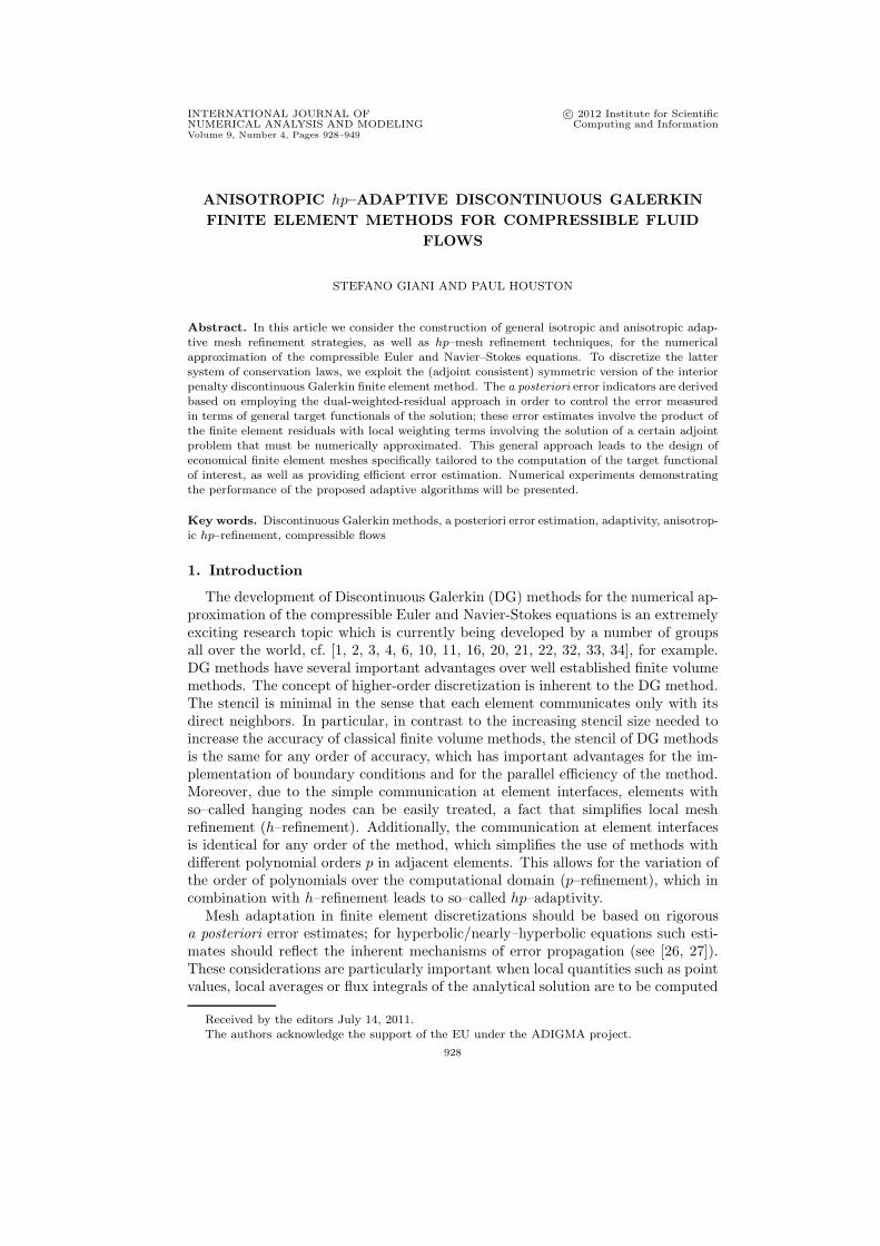
In Figure 12 we show the hp–mesh distributions based on employing a structuredand unstructured initial mesh after 8 and 7 adaptive refinement steps, respectively.In each case we observe that some h–refinement has been undertaken in the vicinityof the boundary layers as we would expect. However, once the h–mesh has ade-quately captured the structure of the primal and adjoint solutions, the hp–adaptivealgorithm subsequently performs p–refinement.

7. Anisotropic hp–mesh adaptation

Finally, in this section we consider the general case of automatically generatinganisotropically refined computational meshes, together with an anisotropic poly-nomial degree distribution. With this in mind, once an element has been select-ed for refinement/derefinement a decision is first made whether to carry out anh-refinement/derefinement or p-enrichment/derefinement based on the techniqueoutlined in Section 6, whereby the analyticity of the solutions u and z is assessedby studying the decay rates of their underlying Legendre coefficients. Once theh– and p–refinement flags have been determined on the basis of the above strat-egy, a decision regarding the type of refinement to be undertaken — isotropic oranisotropic — must be made. Motivated by the work in Section 5, we employa competitive refinement technique, whereby the “optimal” refinement is selectedfrom a series of trial refinements. In the h–version setting, we again exploit thealgorithm outlined in Section 5. For the case when an element has been selected forpolynomial enrichment we consider the p–version counterpart of Algorithm 5.1 andsolve local problems based on increasing the polynomial degrees anisotropically inone direction at a time by one degree, or isotropically by one degree; see [13] fordetails.


(a)

(b)

Figure 12. Example 1 (revisited): hp–Mesh distribution. (a)Structured initial mesh after 8 adaptive refinements; (b) Unstruc-tured initial mesh after 7 adaptive refinements.

7.1. Example 1 (Revisited): Laminar flow around a NACA0012 airfoil.In this section we again consider the test case outlined in Example 1 and againsuppose that the aim of the computation is to calculate the drag coefficient Cd,cf. Section 5.1.1. In Figure 13 we plot the error in the computed target functionalJCd

(·), using a variety of h–/hp–adaptive algorithms against the square–root of thenumber of degrees of freedom on a linear–log scale in the case when an unstructuredinitial mesh is employed. In particular, here we consider the performance of thefollowing adaptive mesh refinement strategies: isotropic h–refinement, anisotropich–refinement, isotropic hp-refinement, anisotropic h–/isotropic p–refinement, andanisotropic hp–refinement. Here, we clearly observe that as the flexibility of theunderlying adaptive strategy is increased, thereby allowing for greater flexibility inthe construction of the finite element space Vh,p, the error in the computed targetfunctional of interest is improved in the sense that the error in the computed val-ue of JCd

(·) is decreased for a fixed number of degrees of freedom. However, wepoint out that in the initial stages of refinement, all of the refinement algorithms


100 150 200 250 300 350 400 450 500

10−4

10−3

Iso h−RefinementAniso h−RefinementIso hp−RefinementAniso h−/Iso p−RefinementAniso hp−Refinement

|JC

d(u

)−JC

d(u

h)|

sqrt(Degrees of freedom)

Figure 13. Example 1 (revisited): Comparison between differentadaptive refinement strategies.

perform in a similar manner. Indeed, it is not until the structure of the underlyinganalytical solution is resolved that we observe the benefits of increasing the com-plexity of the adaptive refinement strategy. Finally, we point out that the latterthree refinement strategies incorporating p–refinement all lead to exponential con-vergence of JCd

(uh) to JCd(u). Figures 14(a) & (b) show the resultant hp–mesh

distribution when employing anisotropic hp–refinement after 5 adaptive steps; here,Figures 14(a) & (b) show the (approximate) polynomial degrees employed in thex– and y–directions, respectively. We observe that anisotropic h–refinement hasbeen employed in order to resolve the boundary layer and anisotropic p-refinementhas been utilized further inside the computational domain. In particular, we noticethat the polynomial degrees have been increased to a higher level in the orthogonaldirection to the curved geometry, as we would expect.

References

[1] F. Bassi and S. Rebay. A high-order accurate discontinuous finite element method for thenumerical solution of the compressible Navier-Stokes equations. J. Comp. Phys., 131:267–279, 1997.

[2] F. Bassi and S. Rebay. High-order accurate discontinuous finite element solution of the 2dEuler equations. J. Comp. Phys., 138:251–285, 1997.

[3] C. Baumann and J. Oden. A discontinuous hp finite element method for the Euler andNavier-Stokes equations. Int. J. Numer. Methods Fluids, 31:79–95, 1999.

[4] C. Baumann and J. Oden. An adaptive-order discontinuous Galerkin method for the solutionof the Euler equations of gas dynamics. Int. J. Numer. Methods Engrg., 47:61–73, 2000.

[5] R. Becker and R. Rannacher. An optimal control approach to a-posteriori error estimationin finite element methods. In A. Iserles, editor, Acta Numerica, pages 1–102. CambridgeUniversity Press, 2001.

[6] V. Dolejsı. On the discontinuous Galerkin method for the numerical solution of the Navier-Stokes equations. Int. J. Numer. Meth. Fluids, 45:1083–1106, 2004.

[7] T. Eibner and J. M. Melenk. An adaptive strategy for hp-FEM based on testing for analyticity.Comput. Mech., 39(5):575–595, 2007.


(a)

(b)

Figure 14. Example 1 (revisited). Mesh distribution after 5adaptive anisotropic hp–refinements, with 2200 elements and 52744degrees of freedom: (a) h–/px–mesh distribution; (b) h–/py–meshdistribution.

[8] K. Eriksson, D. Estep, P. Hansbo, and C. Johnson. Introduction to adaptive methods fordifferential equations. In A. Iserles, editor, Acta Numerica, pages 105–158. Cambridge Uni-versity Press, 1995.

[9] M. Feistauer, J. Felcman, and I. Straskraba. Mathematical and Computational Methods forCompressible Flow. Clarendon Press, Oxford, 2003.

[10] K. Fidkowski and D. Darmofal. A triangular cut-cell adaptive method for high-order dis-cretizations of the compressible Navier-Stokes equations. J. Comput. Phys., 225:1653–1672,2007.


[11] K. Fidkowski, T. Oliver, J. Lu, and D. Darmofal. p-Multigrid solution of high-order discontin-uous Galerkin discretizations of the compressible Navier-Stokes equations. J. Comput. Phys.,207(1):92–113, July 2005.

[12] E. Georgoulis, E. Hall, and P. Houston. Discontinuous Galerkin methods for advection–diffusion–reaction problems on anisotropically refined meshes. SIAM J. Sci. Comput.,30(1):246–271, 2007.

[13] E. Georgoulis, E. Hall, and P. Houston. Discontinuous Galerkin methods on hp–anisotropicmeshes II: A posteriori error analysis and adaptivity. Appl. Numer. Math., 59(9):2179–2194,2009.

[14] S. Giani and P. Houston. High-order hp–adaptive discontinuous Galerkin finite element meth-

ods for compressible fluid flows. In N. Kroll, H. Bieler, H. Deconinck, V. Couallier, H. van derVen, and K. Sorensen, editors, ADIGMA – A European Initiative on the Development ofAdaptive Higher–Order Variational Methods for Aerospace Applications, volume 113 of Noteson Numerical Fluid Mechanics and Multidisciplinary Design, pages 399–411. Springer, 2010.

[15] E. J. C. Hall. Anisotropic Adaptive Refinement For Discontinuous Galerkin Methods. PhDthesis, Department of Mathematics, University of Leicester, 2007.

[16] K. Harriman, P. Houston, B. Senior, and E. Suli. hp–Version discontinuous Galerkin methodswith interior penalty for partial differential equations with nonnegative characteristic form. InC.-W. Shu, T. Tang, and S.-Y. Cheng, editors, Recent Advances in Scientific Computing andPartial Differential Equations. Contemporary Mathematics Vol. 330, pages 89–119. AMS,2003.

[17] R. Hartmann. Adjoint consistency analysis of discontinuous Galerkin discretizations. SIAMJ. Numer. Anal., 45(6):2671–2696, 2007.

[18] R. Hartmann. Numerical analysis of higher order discontinuous Galerkin finite element meth-ods. In H. Deconinck, editor, VKI LS 2008-08: CFD - ADIGMA course on very high orderdiscretization methods, Oct. 13-17, 2008. Von Karman Institute for Fluid Dynamics, RhodeSaint Genese, Belgium, 2008.

[19] R. Hartmann and P. Houston. Adaptive discontinuous Galerkin finite element methods fornonlinear hyperbolic conservation laws. SIAM J. Sci. Comput., 24:979–1004, 2002.

[20] R. Hartmann and P. Houston. Adaptive discontinuous Galerkin finite element methods forthe compressible Euler equations. J. Comput. Phys., 183(2):508–532, 2002.

[21] R. Hartmann and P. Houston. Symmetric interior penalty DG methods for the compressibleNavier–Stokes equations I: Method formulation. Int. J. Num. Anal. Model., 3(1):1–20, 2006.

[22] R. Hartmann and P. Houston. Symmetric interior penalty DG methods for the compressibleNavier–Stokes equations II: Goal–oriented a posteriori error estimation. Int. J. Num. Anal.Model., 3(2):141–162, 2006.

[23] R. Hartmann and P. Houston. An optimal order interior penalty discontinuous Galerkindiscretization of the compressible Navier–Stokes equations. J. Comput. Phys., 227(22):9670–9685, 2008.

[24] R. Hartmann and P. Houston. Error estimation and adaptive mesh refinement for aerody-namic flows. In H. Deconinck, editor, VKI LS 2010-01: 36th CFD/ADIGMA Course onhp-Adaptive and hp-Multigrid Methods, Oct. 26-30, 2009. Von Karman Institute for FluidDynamics, Rhode Saint Genese, Belgium, 2010.

[25] R. Hartmann and T. Leicht. Error estimation and anisotropic mesh refinement for 3d aero-dynamic flow simulations. J. Comput. Phys., 229(19), 2010.

[26] P. Houston, J. Mackenzie, E. Suli, and G. Warnecke. A posteriori error analysis for numericalapproximations of Friedrichs systems. Numer. Math., 82:433–470, 1999.

[27] P. Houston and E. Suli. Local mesh design for the numerical solution of hyperbolic problems.In M. Baines, editor, Numerical methods for Fluid Dynamics VI, ICFD, pages 17–30, 1998.

[28] P. Houston and E. Suli. hp–Adaptive discontinuous Galerkin finite element methods for hy-perbolic problems. SIAM J. Sci. Comput., 23:1225–1251, 2001.

[29] P. Houston and E. Suli. Adaptive finite element approximation of hyperbolic problems. InT. Barth and H. Deconinck, editors, Error Estimation and Adaptive Discretization Methodsin Computational Fluid Dynamics. Lect. Notes Comput. Sci. Engrg., volume 25, pages 269–344. Springer, 2002.

[30] P. Houston and E. Suli. A note on the design of hp–adaptive finite element methods for ellipticpartial differential equations. Comput. Methods Appl. Mech. Engrg., 194(2-5):229–243, 2005.

[31] N. Kroll. ADGIMA – A European project on the development of adaptive higher-order vari-ational methods for aerospace applications. 47th AIAA Aerospace Sciences Meeting, 2009.AIAA 2009-176.


[32] S. Prudhomme, F. Pascal, J. Oden, and A. Romkes. Review of a priori error estimation fordiscontinuous Galerkin methods. TICAM Report 00-27, University of Texas, 2000.

[33] J. van der Vegt and H. van der Ven. Space-time discontinuous Galerkin finite element methodwith dynamic grid motion for inviscid compressible flows, I. General formulation. J. Comp.Phys., 182:546–585, 2002.

[34] K. G. van der Zee. An H1(Ph)-coercive discontinuous Galerkin formulation for the Poissonproblem: 1-d analysis. Master’s thesis, TU Delft, 2004.

School of Mathematical Sciences, University of Nottingham, University Park, Nottingham NG72RD, UK.

E-mail : [email protected]

School of Mathematical Sciences, University of Nottingham, University Park, Nottingham NG72RD, UK.

E-mail : [email protected]

volume 9, number 4, pages 928–949 - ualberta.ca · finite element methods for compressible fluid...

Documents