Visualizing Higher-Layer Features of a Deep Network

Dumitru Erhan, Yoshua Bengio, Aaron Courville, and Pascal VincentDept. IRO, Universite de Montreal

P.O. Box 6128, Downtown Branch, Montreal, H3C 3J7, QC, Canadafirst.last@umontreal.ca

Technical Report 1341Departement d’Informatique et Recherche Operationnelle

June 9th, 2009

AbstractDeep architectures have demonstrated state-of-the-art results in a variety of

settings, especially with vision datasets. Beyond the model definitions and thequantitative analyses, there is a need for qualitative comparisons of the solutionslearned by various deep architectures. The goal of this paper is to find good qualita-tive interpretations of high level features represented by such models. To this end,we contrast and compare several techniques applied on Stacked Denoising Auto-encoders and Deep Belief Networks, trained on several vision datasets. We showthat, perhaps counter-intuitively, such interpretation is possible at the unit level,that it is simple to accomplish and that the results are consistent across varioustechniques. We hope that such techniques will allow researchers in deep architec-tures to understand more of how and why deep architectures work.

1 IntroductionUntil 2006, it was not known how to efficiently learn deep hierarchies of features witha densely-connected neural network of many layers. The breakthrough, by Hintonet al. (2006a), came with the realization that unsupervised models such as RestrictedBoltzmann Machines (RBMs) can be used to initialize the network in a region of theparameter space that makes it easier to subsequently find a good minimum of the su-pervised objective. The greedy, layer-wise unsupervised initialization of a network canalso be carried out by using auto-associators and related models, as shown by Bengioet al. (2007) and Ranzato et al. (2007). Recently, there has been a surge in research ontraining deep architectures: Bengio (2009) gives a comprehensive review.

While quantitative analyses and comparisons of such models exist, and visualiza-tions of the first layer representations are common in the literature, one area where morework needs to be done is the qualitative analysis of representations learned beyond thefirst level.

Some of the deep architectures (such as Deep Belief Nets (Hinton et al., 2006a)) areassociated with a generative procedure, and one could potentially use such a procedure

1

to gain insight into what an individual hidden unit represents. We explore one suchsampling technique here. However, it is sometimes difficult to obtain samples thatcover well the modes of a Boltzmann or RBM distribution, and these sampling-basedvisualizations cannot be applied to to other deep architectures such as those basedon auto-encoders (Bengio et al., 2007; Ranzato et al., 2007; Larochelle et al., 2007;Ranzato et al., 2008; Vincent et al., 2008) or on semi-supervised learning of similarity-preserving embeddings at each level (Weston et al., 2008).

A typical qualitative way of comparing features extracted by a first layer of a deeparchitecture is by looking at the “filters” learned by the model, that is the linear weightsin the input-to-first layer weight matrix, represented in input space. This is particularlyconvenient when the inputs are images or waveforms, which can be visualized. Often,these filters take the shape of stroke detectors, when trained on digit data, or edge detec-tors (Gabor filters) when trained on natural image patches (Hinton et al., 2006a; Hintonet al., 2006b; Osindero & Hinton, 2008; Larochelle et al., 2009). The techniques westudy here also suppose that the input patterns can be displayed and are meaningful forhumans, and we evaluate all of them on image data.

Our aim was to explore ways of visualizing what a unit computes in an arbitrarylayer of a deep network. The goal was to have this visualization in the input space (ofimages), to have an efficient way of computing it, and to make it as general as possible(in the sense of it being applicable to a large class of neural-network-like models). Tothis end, we explore several visualization methods that allow us to gain insight intowhat a particular unit of a neural network represents. We compare and contrast themqualitatively on two image datasets, and we also explore connections between all ofthem.

The main experimental finding of this investigation is very surprising: the responseof an internal unit to input images, as a function in image space, appears to be unimodal,or at least that the maximum is found reliably and consistently for all the random ini-tializations tested. This is interesting because finding this dominant mode is relativelyeasy, and displaying it then provides a good characterization of what the unit does.

2 The modelsWe shall consider two deep architectures as representatives of two families of mod-els encountered in the deep learning literature. The first model is a Deep Belief Net(DBN) (Hinton et al., 2006a), obtained by training and stacking three layers as Re-stricted Boltzmann Machines (RBM) in a greedy manner. This means that we traineda RBM with Contrastive Divergence (Hinton, 2002) on the training data, we fixed theparameters of this RBM, and then trained another RBM to model the hidden layerrepresentations of the first level RBM. This process can be repeated to yield a deeparchitecture that is an unsupervised model of the training distribution. Note that it isalso a generative model of the data and one can easily obtain samples from a trainedmodel. DBNs have been described numerous times in the literature and we use themas described by (Bengio et al., 2007) and (Hinton et al., 2006a); we omit more detailsin favor of describing the other deep architecture.

The second model, by Vincent et al. (2008), is the so-called Stacked DenoisingAuto-Encoder (SDAE). It borrows the greedy principle from DBNs, but uses denois-

2

ing auto-encoders as a building block for unsupervised modeling. An auto-encoderlearns an encoder h(·) and a decoder g(·) whose composition approaches the identityfor examples in the training set, i.e., g(h(x)) ≈ x for x in the training set. The denois-ing auto-encoder is a stochastic variant of the ordinary auto-encoder with the propertythat even with a high capacity model, it cannot learn the identity. Furthermore, itstraining criterion is a variational lower bound on the likelihood of a generative model.It is explicitly trained to denoise a corrupted version of its input. It has been shownon an array of datasets to perform significantly better than ordinary auto-encoders andsimilarly or better than RBMs when stacked into a deep supervised architecture (Vin-cent et al., 2008). Another way to prevent regular auto-encoders with more code unitsthan inputs to learn the identity is to impose sparsity on the code (Ranzato et al., 2007;Ranzato et al., 2008). The activation maximization technique presented below is appli-cable to any trained deep neural network, and we evaluate it on networks obtained bystacking RBMs and denoising auto-encoders.

We now summarize the training algorithm of the Stacked Denoising Auto-Encoders.More details are given by Vincent et al. (2008). Each denoising auto-encoder operateson its inputs x, either the raw inputs or the outputs of the previous layer. The denoisingauto-encoder is trained to reconstruct x from a stochastically corrupted (noisy) trans-formation of it. The output of each denoising auto-encoder is the “code vector” h(x).In our experiments h(x) = sigmoid(b + Wx) is an ordinary neural network layer,with hidden unit biases b, weight matrix W , and sigmoid(a) = 1/(1 + exp(−a))(applied element-wise on a vector a). Let C(x) represent a stochastic corruption ofx. As done by Vincent et al. (2008), we set Ci(x) = xi or 0, with a random subset(of a fixed size) selected for zeroing. We have also considered a salt and pepper noise,where we select a random subset of a fixed size and set Ci(x) = Bernoulli(0.5). The“reconstruction” is obtained from the noisy input with x = sigmoid(c+WT h(C(x))),using biases c and the transpose of the feed-forward weights W . In the experimentson images, both the raw input xi and its reconstruction xi for a particular pixel i canbe interpreted as a Bernoulli probability for that pixel: the probability of painting thepixel as black at that location. We denote ∂KL(x||x) =

∑i ∂KL(xi||xi) the sum

of component-wise KL divergences between the Bernoulli probability distributions as-sociated with each element of x and its reconstruction probabilities x: KL(x||x) =−

∑i (xilog xi + (1− xi) log (1− xi)). The Bernoulli model only makes sense when

the input components and their reconstruction are in [0, 1]; another option is to use aGaussian model, which corresponds to a Mean Squared Error (MSE) criterion.

For each unlabeled example x, a stochastic gradient estimator is then obtained bycomputing ∂KL(x||x)/∂θ for θ = (b, c,W ). The gradient is stochastic because ofsampling example x and because of the stochastic corruption C(x). Stochastic gradientdescent θ ← θ − ε · ∂KL(x||x)/∂θ is then performed with learning rate ε, for a fixednumber of pre-training iterations.

3

3 Maximizing the activationThe first idea is simple: we look for input patterns of bounded norm which maximizethe activation of a given hidden unit1; since the activation function of a unit in the firstlayer is a linear function of the input, in the case of the first layer, this input pattern isproportional to the filter itself.

The reasoning behind this idea is that a pattern to which the unit is respondingmaximally could be a good first-order representation of what a unit is doing. Onesimple way of doing this is to find, for a given unit, the input sample(s) (from either thetraining or the test set) that give rise to the highest activation of the unit. Unfortunately,this still leaves us with the problem of choosing how many samples to keep for each unitand the problem of how to “combine” these samples. Ideally, we would like to find outwhat these samples have in common. Furthermore, it may be that only some subsets ofthe input vector contribute to the high activation, and it is not easy to determine whichby inspection.

Note that we restricted ourselves needlessly to searching for an input pattern fromthe training or test sets. We can take a more general view and see our idea—maximizingthe activation of a unit—as an optimization problem. Let θ denote our neural networkparameters (weights and biases) and let hij(θ,x) be the activation of a given unit ifrom a given layer j in the network; hij is a function of both θ and the input samplex. Assuming a fixed θ (for instance, the parameters after training the network), we canview our idea as looking for

x∗ = arg maxx s.t. ||x||=ρ

hij(θ,x).

This is, in general, a non-convex optimization problem. But it is a problem for whichwe can at least try to find a local minimum. This can be done most easily by performingsimple gradient ascent in the input space, i.e. computing the gradient of hij(θ,x) andmoving x in the direction of this gradient2.

Two scenarios are possible: the same (qualitative) minimum is found when startingfrom different random initializations or two or more local minima are found. In bothcases, the unit can then be characterized by the minimum or set of minima found. Inthe latter case, one can either average the results, or choose the one which maximizesthe activation, or display all the local minima obtained to characterize that unit.

This optimization technique (we will call it “activation maximization”) is applica-ble to any network in which we can compute the above gradients. Like any gradientdescent technique, it does involve a choice of hyperparameters: the learning rate anda stopping criterion (the maximum number of gradient ascent updates, in our experi-ments).

4 Sampling from a unit of a Deep Belief NetworkConsider a Deep Belief Network with j layers, as described in Section 2. In particular,layers j−1 and j form an RBM from which we can sample using block Gibbs sampling,

1The total sum of the input to the unit from the previous layer plus its bias.2Since we are trying to maximize hij .

4

which successively samples from p(hj−1|hj) and p(hj |hj−1), denoting by hj the bi-nary vector of units from layer j. Along this Markov chain, we propose to “clamp”unit hij , and only this unit, to 1. We can then sample inputs x by performing ancestraltop-down sampling in the directed belief network going from layer j − 1 to the input,in the DBN. This will produce a distribution that we shall denote by pj(x|hij = 1)where hij is the unit that is clamped, and pj denotes the depth-j DBN containing onlythe first j layers. This procedure is similar to and inspired from experiments by Hintonet al. (2006a), where the top layer RBM is trained on the representations learned bythe previous RBM and the label as a one-hot vector; in that case, one can “clamp” thelabel vector to a particular configuration and sample from a particular class distributionp(x|class = k).

In essence, we use the distribution pj(x|hij = 1) to characterize hij . In analogy toSection 3, we can characterize the unit by many samples from this distribution or sum-marize the information by computing the expectation E[x|hij = 1]. This method has,essentially, no hyperparameters except the number of samples that we use to estimatethe expectation. It is relatively efficient provided the Markov chain at layer j mixeswell (which is not always the case, unfortunately).

There is an interesting link between the method of maximizing the activation andE[x|hij = 1]. By definition, E[x|hij = 1] =

∫xpj(x|hij = 1)dx. If we consider the

extreme case where the distribution concentrates at x+, pj(x|hij = 1) ≈ δx+(x), thenthe expectation is E[x|hij = 1] = x+.

On the other hand, when applying the activation maximization technique to a DBN,we are approximately 3 looking for arg maxx p(hij = 1|x), since this probabilityis monotonic in the activation of unit hij . Using Bayes’ rule and the concentrationassumption about p(x|hij = 1), we find that

p(hij = 1|x) =p(x|hij = 1)p(hij = 1)

p(x)=

δx+(x)p(hij = 1)p(x)

This is zero everywhere except at x+ so under our assumption, arg maxx p(hij =1|x) = x+.

More generally, one can show that if p(x|hij = 1) concentrates sufficiently aroundx+ compared to p(x), then the two methods (expected value over samples vs activa-tion maximization) should produce very similar results. Generally speaking, it is easyto imagine how such an assumption could be untrue because of the nonlinearities in-volved. In fact, what we observe is that although the samples or their average may looklike training examples, the images obtained by activation maximization look more likeimage parts, which may be a more accurate representation of what the particular unitsdoes (by opposition to all the other units involved in the sampled patterns).

5 Linear combination of previous layers’ filtersLee et al. (2008) showed one way of visualizing what the units in the second hiddenlayer of a network are responding to. They made the assumption that a unit can be

3because of the approximate optimization and because the true posteriors are intractable for higher layers,and only approximated by the corresponding neural network unit outputs.

5

characterized by the filters of the previous layer to which it is most strongly connected4.By taking a weighted linear combination of the previous layer filters—where the weightof the filters is its weight to the unit considered—they show that a Deep Belief Networkwith sparsity constraints on the activations, trained on natural images, will tend to learn“corner detectors” at the second layer. Lee et al. (2009) used an extended version ofthis method for visualizing units of the third layer: by simply weighing the “filters”found at the second layer by their connections to the third layer, and choosing againthe largest weights.

Such a technique is simple and efficient. One disadvantage is that it is not clearhow to automatically choose the appropriate number of filters to keep at each layer.Moreover, by selecting only the very few most strongly connected filters from the firstlayer, one can potentially get a misleading picture, since one is essentially ignoring therest of the previous layer units. Finally, this method also bypasses the nonlinearitiesbetween layers, which may be an important part of the model. One motivation for thispaper is to validate whether the patterns obtained by Lee et al. (2008) are similar tothose obtained by the other methods explored here.

One should note that there is indeed a link between the gradient updates for max-imizing the activation of a unit and finding the linear combination of weights as de-scribed by Lee et al. (2009). Take, for instance hi2, i.e. the activation of unit ifrom layer 2 with hi2 = v′sigmoid(Wx), with v being the unit’s weights and Wbeing the first layer weight matrix. Then ∂hi2/∂x = v′diag(sigmoid(Wx) ∗ (1 −sigmoid(Wx)))W , where ∗ is the element-wise multiplication, diag is the operatorthat creates a diagonal matrix from a vector, and 1 is a vector filled with ones. If theunits of the first layer do not saturate, then ∂hi2/∂x points roughly in the direction ofv′W , which can be approximated by taking the terms with the largest absolute valueof vi.

6 Experiments6.1 Data and setupWe used two datasets: the first is an extended version of the MNIST digit classificationdataset, by Loosli et al. (2007), in which elastic deformations of digits are generatedstochastically. We used 2.5 million examples as training data, where each example isa 28 × 28 gray-scale image. The second is a collection of 100000 12 × 12 patchesof natural images, generated from the collection of whitened natural image patches byOlshausen and Field (1996).

The visualization procedures were tested on the models described in Section 2:Deep Belief Nets (DBNs) and Stacked Denoising Auto-encoders (SDAE). The hyper-parameters are: unsupervised and supervised learning rates, number of hidden unitsper layer, and the amount of noise in the case of SDAE; they were chosen to minimize

4i.e. whose weight to the upper unit is large in magnitude

6

the classification error on MNIST5 or the reconstruction error6 on natural images, fora given validation set. For MNIST, we show the results obtained after unsupervisedtraining only; this allows us to compare all the methods (since we cannot sample froma DBN after supervised fine-tuning). For the SDAE, we used salt and pepper noiseas a corruption technique, as opposed to the zero-masking noise described by Vincentet al. (2008): such noise seems to better model natural images. For both SDAE andDBN we used a Gaussian input layer when modeling natural images; these are moreappropriate than the standard Bernoulli units, given the distribution of pixel grey levelsin such patches (Bengio et al., 2007; Larochelle et al., 2009).

In the case of activation maximization (Section 3), the procedure is as follows for agiven unit from either the second or the third layer: we initialize x to a vector of 28×28or 12 × 12 dimensions in which each pixel is sampled independently from a uniformover [0; 1]. We then compute the gradient of the activation of the unit w.r.t. x and makea step in the gradient direction. The gradient updates are continued until convergence,i.e. until the activation function does not increase by much anymore. Note that aftereach gradient update, the current estimate of x∗ is re-normalized to the average normof examples from the respective dataset7. Interestingly, the same optimal value (i.e. theone that seems to maximize activation) for the learning rate of the gradient ascent worksfor all the units from the same layer.

Sampling from a DBN is done as described in Section 4, by running the randomly-initialized Markov chain and top-down sampling every 100 iterations. In the case ofthe method described in Section 5, the (subjective) optimal number of previous layerfilters was taken to be 100.

6.2 Activation MaximizationWe begin by the analysis of the activation maximization method. Figures 1 and 2contain the results of the optimization of units from the 2nd and 3rd layers of a DBNand an SDAE, along with the first layer filters. Figure 1 shows such an analysis forMNIST and Figure 2 shows it for the natural image data.

To test the dependence of this gradient ascent on the initial conditions, 9 differentrandom initializations were tried. The retained “filter” corresponding to each unit isthe one (out of the 9 random initializations) which maximizes the activation. In thesame figures we also show the variations found by the different random initializationsfor a given unit from the 3rd layer. Surprisingly, most random initializations yieldroughly the same prominent input pattern. Moreover, we measured the maximum

5We are indeed choosing our hyperparameters based on the supervised objective. This objective is com-puted by using the unsupervised networks as initial parameters for supervised backpropagation. We chose toselect the hyperparameters based on the classification error because for this problem we do have an objectivecriterion for comparing networks, which is not the case for the natural image data.

6For RBMs, the reconstruction error is obtained by treating the RBM as an auto-encoder and computinga deterministic value using either the KL divergence or the MSE, as appropriate. The reconstruction error ofthe first layer RBM is used for model selection.

7There is no constraint that the resulting values in x∗ be in the domain of the training/test set values.For instance, we experimented with making sure that the values of x∗ are in [0; 1] (for MNIST), but thisproduced worse results. On the other hand, the goal is to find a “filter”-like result and a constraint that this“filter” is strictly in the same domain as the input image may not be necessary.

7

Figure 1: Activation maximization applied on MNIST. On the left side: visualization of 36units from the first (1st column), second (2nd column) and third (3rd column) hidden layers of aDBN (top) and SDAE (bottom), using the technique of maximizing the activation of the hiddenunit. On the right side: 4 examples of the solutions to the optimization problem for units in the3rd layer of the SDAE, from 9 random initializations.

values for the activation function to be quite close to each other (not shown). Suchresults are relatively surprising, given that, generally speaking, the activation functionof a third layer unit is a highly non-convex function of its input. Therefore, either we areconsistently lucky or, at least in this particular case (a network trained on MNIST digitsor natural images), the activation functions of the units tend to be more “unimodal”.

To further test the robustness of the activation maximizationmethod, we perform a sensitivity analysis in order to testwhether the units are selective to these patterns found by theoptimization routine, and whether these patterns strongly ac-tivate other units as well. The figure on the right shows thepost-sigmoidal activation of unit j (columns) when the inputto the network is the “optimal” pattern i (rows), found byour gradient procedure for unit i, normalized across columnsin order to eliminate the effect of units that are activated forvery many patterns in general. The strong values on the di-agonal suggest that the results of the optimization have un-covered patterns that are mostly specific to a particular unit.One important point is that, qualitatively speaking, the filters at the 3rd layer look

interpretable and quite complex. For MNIST, some look like pseudo-digits. In thecase of natural images, we can observe grating filters at the second layer of DBNsand complicated units that detect, for instance, corners at the second and third layer ofSDAE; some of the units have the same characteristics that we would associate withso-called complex cells. It suggests that higher level units did indeed learn meaningfulcombinations of lower level features.

Note that the first layer filters obtained by the SDAE when trained on natural im-ages are Gabor-like features. It is interesting that in the case of DBN, the filters thatminimized the reconstruction error8, i.e. those that are pictured in Figure 2 (top-left cor-ner), do not have the same low-frequency and sparsity properties like the ones found

8Which is only a proxy for the actual objective function that is minimized by a stack of RBMs.

8

by the first-level denoising auto-encoder9. Yet at the second layer, the filters found byactivation maximization are a mixture of Gabor-like features and grating filters. Thisshows that appearances can be deceiving: we might have dismissed the RBM whoseweights are shown in Figure 2 as a bad model of natural images had we looked only atthe first layer filters, but the global qualitative assessment of this model, which includesthe visualization of the second and third layers, points to the fact that the 3-layer DBNis in effect learning something quite interesting.

Figure 2: On the left side: Visualization of 144 units from the first (1st column), second (2ndcolumn) and third (3rd column) hidden layers of a DBN (top) and an SDAE (bottom), using thetechnique of maximizing the activation of the hidden unit. On the right side: 4 examples of thesolutions to the optimization problem for units in the 3rd layer of the SDAE, subject to 9 randominitializations.

6.3 Sampling a unitOf note is the fact that unlike the results of the activation maximization method, thesamples are much more likely to be part of the underlying distribution of examples(digits or patches). The activation maximization method seems to produce featuresand it is up to us to decide which examples would “fit” these features; the samplingmethod produces examples and it lets us decide which features these examples have incommon. In this respect, the two techniques serve complementary purposes.

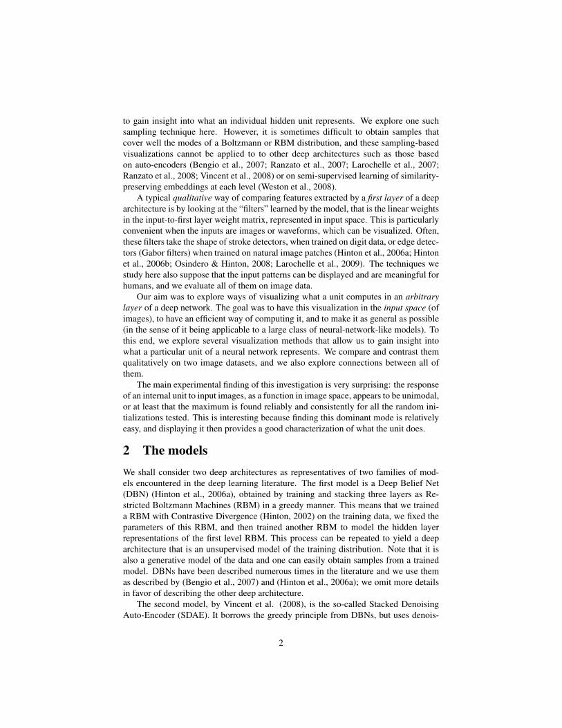
6.4 Comparison of methodsIn Figure 4, we can see a comparison of the three techniques, including the linearcombination method. The methods are tested on the second layer of a DBN trainedon MNIST. In the above, we noted links between the three techniques. The experi-ments show that many of the filters found by the three methods share some features,but have a different nature. Unfortunately, we do not have an objective measure thatwould allow us to compare the three methods, but visually the activation maximization

9It is possible to obtain Gabor-like features with RBMs—work by Osindero and Hinton (2008) showsthat—but in our case these filters were never those that minimized the reconstruction error of an RBM. Thispoints to a larger issue: it appears that using different learning rates for Contrastive Divergence learning willinduce features that are qualitatively different, depending on the value of the learning rate.

9

We now turn to the sampling techniquedescribed in Section 4. Figure 3 showssamples obtained by clamping a secondlayer unit to 1; both MNIST and natural im-age patches are considered. In the case ofnatural image patches, the distributions areroughly unimodal, in that the samples areof the same pattern, for a given unit. ForMNIST, the situation is slightly more deli-cate: there seem to be one or two modes foreach unit. The average input (the expecta-tion of the distribution), as seen in Figure 4,then looks like a digit or a superposition oftwo digits.

Figure 3: Visualization of 6 units from the sec-ond hidden layer of a DBN trained on MNIST(left) and natural image patches (right). The vi-sualizations are produced by sampling from theDBN and clamping the respective unit to 1. Eachunit’s distribution is a row of samples; the meanof each row is in the first column of Figure 4(left).

method seems to produce more interesting results: by comparison, the average sam-ples from the DBN are almost always in the shape of a digit (for MNIST), while thelinear combination method seems to find only parts of the features that are found byactivation maximization, which tends to find sharper patterns.

6.5 LimitationsWe tested the activation maximization procedure on image patches of 20 × 20 pixels(instead of 12×12) and found that the optimization does not converge to a single globalminimum. Moreover, the input distribution that is sampled with the units clamped to1 has many different modes and its expectation is not meaningful or interpretable any-more. We posit that these methods break down because of the complexity of the inputdistribution: both MNIST and 12 × 12 image patches are relatively simple distribu-tions to model and this could be the reason these methods work in the first place. It isperhaps unrealistic to expect that as we scale the datasets to larger and larger images,one could still find a simple representation of a higher layer unit. We should note,however, that there is a recent trend of developing convolutional versions of deep ar-chitectures (Kavukcuoglu et al., 2009; Lee et al., 2009; Desjardins & Bengio, 2008): itis likely that one will be able to apply the same techniques in that scenario and still beable to recover good visualizations, even with large inputs.

7 Conclusions and Future WorkWe started from a simple premise: to better understand the solution that is learned andrepresented by a deep architecture, by investigating the response of individual units inthe network. Like the analysis of individual neurons in the brain by neuroscientists,this approach has limitations, but we hope that such visualization techniques can helpunderstand the nature of the functions learned by the network.

We presented three simple techniques: activation maximization and sampling froma unit are both new (to the best of our knowledge), while the linear combination tech-nique had been previously published. We showed the intuitive similarities between

10

Figure 4: Visualization of 36 units from the second hidden layer of a DBN trained on MNIST(top) and 144 units from the second hidden layer of a DBN trained on natural image patches(bottom). Left: sampling with clamping, Centre: linear combination of previous layer filters,Right: maximizing the activation of the unit. Black is negative, white is positive and gray iszero.

them and compared and contrasted them on two well-known datasets. Our results con-firm the intuitions that we had about the hierarchical representations learned by deeparchitectures: namely that the higher layer units represent features that are (meaning-fully) more complicated and that correspond to combinations of features of the lowerlayers. We have also found that the two deep architectures considered learn quite dif-ferent features.

The same procedures can be applied to the weights obtained after supervised learn-ing and the observations are similar: convergence occurs and features seem more com-plicated at higher layers. In the future, we would like to use such visualization toolsto compare the features learned by these networks after supervised learning, in orderto better understand the differences in test error and to further understand the influenceof unsupervised initialization in training deep models. We will also extend our resultsby performing experiments with other datasets and models, such as Convolutional Net-works applied to higher-resolution natural images. Finally, we would like to comparethe behaviour of higher level units in a deep network to features that are presumed tobe encoded by the higher levels of the visual cortex.

ReferencesBengio, Y. (2009). Learning deep architectures for AI. Foundations and Trends in

Machine Learning, to appear.

11

Bengio, Y., Lamblin, P., Popovici, D., & Larochelle, H. (2007). Greedy layer-wisetraining of deep networks. Advances in Neural Information Processing Systems 19(pp. 153–160). MIT Press.

Desjardins, G., & Bengio, Y. (2008). Empirical evaluation of convolutional RBMs forvision (Technical Report 1327).

Hinton, G. E. (2002). Training products of experts by minimizing contrastive diver-gence. Neural Computation, 14, 1771–1800.

Hinton, G. E., Osindero, S., & Teh, Y. (2006a). A fast learning algorithm for deepbelief nets. Neural Computation, 18, 1527–1554.

Hinton, G. E., Osindero, S., Welling, M., & Teh, Y. (2006b). Unsupervised discoveryof non-linear structure using contrastive backpropagation. Cognitive Science, 30.

Kavukcuoglu, K., Ranzato, M., Fergus, R., & LeCun, Y. (2009). Learning invariantfeatures through topographic filter maps. Proc. International Conference on Com-puter Vision and Pattern Recognition (CVPR’09). IEEE.

Larochelle, H., Bengio, Y., Louradour, J., & Lamblin, P. (2009). Exploring strategiesfor training deep neural networks. Journal of Machine Learning Research, 10, 1–40.

Larochelle, H., Erhan, D., Courville, A., Bergstra, J., & Bengio, Y. (2007). An em-pirical evaluation of deep architectures on problems with many factors of variation.ICML 2007: Proceedings of the Twenty-fourth International Conference on MachineLearning (pp. 473–480). Corvallis, OR: Omnipress.

Lee, H., Ekanadham, C., & Ng, A. (2008). Sparse deep belief net model for visual areaV2. In J. C. Platt, D. Koller, Y. Singer and S. Roweis (Eds.), Advances in neuralinformation processing systems 20. Cambridge, MA: MIT Press.

Lee, H., Grosse, R., Ranganath, R., & Ng, A. Y. (2009). Convolutional deep beliefnetworks for scalable unsupervised learning of hierarchical representations. In Icml2009: Proceedings of the twenty-sixth international conference on machine learn-ing. Montreal (Qc), Canada.

Loosli, G., Canu, S., & Bottou, L. (2007). Training invariant support vector machinesusing selective sampling. In L. Bottou, O. Chapelle, D. DeCoste and J. Weston(Eds.), Large scale kernel machines, 301–320. Cambridge, MA.: MIT Press.

Olshausen, B. A., & Field, D. J. (1996). Emergence of simple-cell receptive fieldproperties by learning a sparse code for natural images. Nature, 381, 607–609.

Osindero, S., & Hinton, G. E. (2008). Modeling image patches with a directed hier-archy of markov random field. Neural Information Processing Systems Conference(NIPS) 20.

Ranzato, M., Boureau, Y.-L., & LeCun, Y. (2008). Sparse feature learning for deep be-lief networks. Advances in Neural Information Processing Systems 20. Cambridge,MA: MIT Press.

12

Ranzato, M., Poultney, C., Chopra, S., & LeCun, Y. (2007). Efficient learning ofsparse representations with an energy-based model. Advances in Neural InformationProcessing Systems 19 (pp. 1137–1144). MIT Press.

Vincent, P., Larochelle, H., Bengio, Y., & Manzagol, P.-A. (2008). Extracting andcomposing robust features with denoising autoencoders. ICML 2008: Proceedingsof the Twenty-fifth International Conference on Machine Learning (pp. 1096–1103).

Weston, J., Ratle, F., & Collobert, R. (2008). Deep learning via semi-supervisedembedding. Proceedings of the Twenty-fifth International Conference on MachineLearning (ICML 2008).

13