visualization techniques for computational · university of california santa cruz visualization...
TRANSCRIPT

UNIVERSITY OF CALIFORNIA
SANTA CRUZ
VISUALIZATION TECHNIQUES FOR COMPUTATIONAL
MECHANICS
A dissertation submitted in partial satisfaction of therequirements for the degree of
DOCTOR OF PHILOSOPHY
in
COMPUTER SCIENCE
by
Alisa Gail Neeman
December 2009
The Dissertation of Alisa Gail Neemanis approved:
Professor Alex Pang, Chair
Professor Boris Jeremic
Professor Suresh Lodha
Tyrus MillerVice Provost and Dean of Graduate Studies

Copyright c! by
Alisa Gail Neeman
2009

Table of Contents
List of Figures vii
List of Tables x
Abstract xi
Dedication xii
Acknowledgments xiii
1 Introduction 1
1.1 Main Contributions . . . . . . . . . . . . . . . . . . . . . . . . . . . . . . 21.2 Auxiliary Artifacts . . . . . . . . . . . . . . . . . . . . . . . . . . . . . . 31.3 Dissertation Organization . . . . . . . . . . . . . . . . . . . . . . . . . . 3
2 Tensor Basics 4
2.1 Einstein Notation . . . . . . . . . . . . . . . . . . . . . . . . . . . . . . . 52.2 Common Operations . . . . . . . . . . . . . . . . . . . . . . . . . . . . . 6
2.2.1 Inner Product . . . . . . . . . . . . . . . . . . . . . . . . . . . . . 62.2.2 Scalar Multiplication . . . . . . . . . . . . . . . . . . . . . . . . . 72.2.3 Matrix Multiplication . . . . . . . . . . . . . . . . . . . . . . . . 72.2.4 Double Contraction . . . . . . . . . . . . . . . . . . . . . . . . . 72.2.5 Outer Product . . . . . . . . . . . . . . . . . . . . . . . . . . . . 82.2.6 Eigen-Decomposition . . . . . . . . . . . . . . . . . . . . . . . . . 9
2.3 Properties of Tensors . . . . . . . . . . . . . . . . . . . . . . . . . . . . . 92.3.1 Symmetry . . . . . . . . . . . . . . . . . . . . . . . . . . . . . . . 92.3.2 Symmetry of Second-Order Tensors . . . . . . . . . . . . . . . . 102.3.3 Symmetry of Fourth-Order Tensors . . . . . . . . . . . . . . . . . 112.3.4 Positive-Definiteness . . . . . . . . . . . . . . . . . . . . . . . . . 112.3.5 Singularity . . . . . . . . . . . . . . . . . . . . . . . . . . . . . . 12
iii

3 Continuum Mechanics and Solid Modeling 13
3.1 Hooke’s Law - the Basic Constitutive Equation in 1D . . . . . . . . . . . 143.2 Stress and Strain Tensors . . . . . . . . . . . . . . . . . . . . . . . . . . 15
3.2.1 Two Useful Scalars Describing Stress . . . . . . . . . . . . . . . . 163.3 Two and Three Dimensional Continuum Solids . . . . . . . . . . . . . . 17
3.3.1 Sti!ness versus Compliance . . . . . . . . . . . . . . . . . . . . . 173.3.2 Important Solid Material Constants . . . . . . . . . . . . . . . . 173.3.3 Intuition . . . . . . . . . . . . . . . . . . . . . . . . . . . . . . . . 19
3.4 Sti!ness As A Tensor . . . . . . . . . . . . . . . . . . . . . . . . . . . . 203.4.1 Elastic Isotropic Materials . . . . . . . . . . . . . . . . . . . . . . 213.4.2 3D case . . . . . . . . . . . . . . . . . . . . . . . . . . . . . . . . 223.4.3 Anisotropy . . . . . . . . . . . . . . . . . . . . . . . . . . . . . . 22
3.5 Elasto-plasticity . . . . . . . . . . . . . . . . . . . . . . . . . . . . . . . . 233.5.1 Nonlinear Elastic Models . . . . . . . . . . . . . . . . . . . . . . 26
4 Related Work 27
4.1 Vector Fields . . . . . . . . . . . . . . . . . . . . . . . . . . . . . . . . . 294.1.1 Streamlines . . . . . . . . . . . . . . . . . . . . . . . . . . . . . . 294.1.2 Flow Topology of Vector Fields . . . . . . . . . . . . . . . . . . . 30
4.2 Second-Order Tensor Fields . . . . . . . . . . . . . . . . . . . . . . . . . 314.2.1 Hyperstreamlines . . . . . . . . . . . . . . . . . . . . . . . . . . . 314.2.2 Glyphs . . . . . . . . . . . . . . . . . . . . . . . . . . . . . . . . . 354.2.3 Seismology Glyphs . . . . . . . . . . . . . . . . . . . . . . . . . . 40
4.3 Fourth-Order Tensors . . . . . . . . . . . . . . . . . . . . . . . . . . . . 434.3.1 HOT-lines . . . . . . . . . . . . . . . . . . . . . . . . . . . . . . . 44
5 Unrolling Tensors To Matrices 47
5.1 Basis . . . . . . . . . . . . . . . . . . . . . . . . . . . . . . . . . . . . . . 485.2 Matrix and Vector Representation . . . . . . . . . . . . . . . . . . . . . 49
6 Decomposition of Fourth-Order Sti!ness Tensors for Visualization 52
6.1 Sti!ness Changes . . . . . . . . . . . . . . . . . . . . . . . . . . . . . . . 536.1.1 Elastic Behavior . . . . . . . . . . . . . . . . . . . . . . . . . . . 546.1.2 Elastic-Plastic Behavior . . . . . . . . . . . . . . . . . . . . . . . 546.1.3 Hardening and Softening . . . . . . . . . . . . . . . . . . . . . . 556.1.4 Localized Failure . . . . . . . . . . . . . . . . . . . . . . . . . . . 57
6.2 Related Work on Decomposition . . . . . . . . . . . . . . . . . . . . . . 576.3 Our Approach . . . . . . . . . . . . . . . . . . . . . . . . . . . . . . . . . 58
6.3.1 Method Constraints . . . . . . . . . . . . . . . . . . . . . . . . . 596.3.2 Method Details . . . . . . . . . . . . . . . . . . . . . . . . . . . . 60
6.4 Polar Decomposition Algorithm . . . . . . . . . . . . . . . . . . . . . . . 656.4.1 Simple Polar Decomposition for Positive-Definite Matrices . . . . 666.4.2 Algorithm for a Zero or Near-Zero Eigenvalue . . . . . . . . . . . 66
iv

6.4.3 Additional Details . . . . . . . . . . . . . . . . . . . . . . . . . . 676.5 Analysis of Rotation Representation . . . . . . . . . . . . . . . . . . . . 68
6.5.1 Origin of Dyad Components . . . . . . . . . . . . . . . . . . . . . 696.5.2 Justification for Rotation . . . . . . . . . . . . . . . . . . . . . . 70
6.6 Results . . . . . . . . . . . . . . . . . . . . . . . . . . . . . . . . . . . . . 726.6.1 Testing Methods . . . . . . . . . . . . . . . . . . . . . . . . . . . 736.6.2 Tests of Material Models . . . . . . . . . . . . . . . . . . . . . . . 73
7 Visualization of Second-Order, 3D, Non-Positive-Definite Symmetric
Tensors 77
7.1 Stress and Strain Tensor Features . . . . . . . . . . . . . . . . . . . . . . 787.1.1 Stresses in Geomaterial Solids . . . . . . . . . . . . . . . . . . . . 79
7.2 Reynolds Glyphs . . . . . . . . . . . . . . . . . . . . . . . . . . . . . . . 807.2.1 Graphical Issue . . . . . . . . . . . . . . . . . . . . . . . . . . . . 817.2.2 Associated Scalar Color Fields . . . . . . . . . . . . . . . . . . . 827.2.3 Experiment . . . . . . . . . . . . . . . . . . . . . . . . . . . . . . 84
7.3 Plane-In-A-Box Glyph . . . . . . . . . . . . . . . . . . . . . . . . . . . . 887.3.1 Data Structures and Algorithms . . . . . . . . . . . . . . . . . . 897.3.2 Associated Scalar Color Fields . . . . . . . . . . . . . . . . . . . 967.3.3 Seismic Moment Tensors . . . . . . . . . . . . . . . . . . . . . . . 967.3.4 Data Meaning . . . . . . . . . . . . . . . . . . . . . . . . . . . . 1037.3.5 Data Representation . . . . . . . . . . . . . . . . . . . . . . . . . 1037.3.6 Results . . . . . . . . . . . . . . . . . . . . . . . . . . . . . . . . 1047.3.7 Conclusions . . . . . . . . . . . . . . . . . . . . . . . . . . . . . . 110
7.4 Continuous Visualization . . . . . . . . . . . . . . . . . . . . . . . . . . 1117.4.1 Interpolating to a Regular Mesh . . . . . . . . . . . . . . . . . . 1117.4.2 Creating an Eigenvector Field . . . . . . . . . . . . . . . . . . . . 1127.4.3 Future Work . . . . . . . . . . . . . . . . . . . . . . . . . . . . . 114
8 Documentation of VEES Software 117
8.1 Introduction . . . . . . . . . . . . . . . . . . . . . . . . . . . . . . . . . . 1178.2 User Guide . . . . . . . . . . . . . . . . . . . . . . . . . . . . . . . . . . 119
8.2.1 Linux Setup and Getting Started . . . . . . . . . . . . . . . . . . 1198.2.2 Using VEES . . . . . . . . . . . . . . . . . . . . . . . . . . . . . 1198.2.3 Main Window . . . . . . . . . . . . . . . . . . . . . . . . . . . . . 1208.2.4 Filtering . . . . . . . . . . . . . . . . . . . . . . . . . . . . . . . . 1218.2.5 Color Map Range Adjustment . . . . . . . . . . . . . . . . . . . 1218.2.6 Element Window . . . . . . . . . . . . . . . . . . . . . . . . . . . 1228.2.7 Integration Point Window . . . . . . . . . . . . . . . . . . . . . . 1228.2.8 Capturing Images and Data for Post-Processing . . . . . . . . . . 124
8.3 Architecture . . . . . . . . . . . . . . . . . . . . . . . . . . . . . . . . . . 1258.3.1 Model-View-Controller . . . . . . . . . . . . . . . . . . . . . . . . 1268.3.2 Strategy Pattern . . . . . . . . . . . . . . . . . . . . . . . . . . . 127
v

8.3.3 Command Pattern . . . . . . . . . . . . . . . . . . . . . . . . . . 1288.3.4 Memento . . . . . . . . . . . . . . . . . . . . . . . . . . . . . . . 129
8.4 OpenSees Example . . . . . . . . . . . . . . . . . . . . . . . . . . . . . . 130
9 Conclusion 137
Bibliography 138
vi

List of Figures
3.1 Spring response under applied force . . . . . . . . . . . . . . . . . . . . . 143.2 Stress tensor components. . . . . . . . . . . . . . . . . . . . . . . . . . . 163.3 Triaxial Stress. . . . . . . . . . . . . . . . . . . . . . . . . . . . . . . . . 193.4 Von Mises yield surface in stress space. . . . . . . . . . . . . . . . . . . . 25
4.1 Critical point classification in a 2D flow field. R: real eigenvalue. I:Imaginary eigenvalue. Image source: [26]. . . . . . . . . . . . . . . . . . 31
4.2 Hyperstreamlines. Figure source: [16] . . . . . . . . . . . . . . . . . . . . 324.3 Double degenerate lines in a tensor field. Figure source: [83] . . . . . . . 334.4 Hedgehog glyphs in a tensor field resulting from a double point load
applied to a volume. Red represents tension, and green, compression.Figure source: [37] . . . . . . . . . . . . . . . . . . . . . . . . . . . . . . 36
4.5 Superquadric tensor glyphs. Figure source: [44] . . . . . . . . . . . . . . 374.6 Reynolds Glyph for stress tensor with eigenvalues (-0.816, 0.408,0.408).
Eigenvectors coincide with Cartesian Axes. Red is X, green is Y and blueis Z. . . . . . . . . . . . . . . . . . . . . . . . . . . . . . . . . . . . . . . 38
4.7 HWY glyph for illustrating shear stress, eigenvalues listed in illustration.Image source:[25]. . . . . . . . . . . . . . . . . . . . . . . . . . . . . . . . 39
4.8 Lame stress ellipsoids for single point load applied on top center of volume(generated with VTK[67]). . . . . . . . . . . . . . . . . . . . . . . . . . . 39
4.9 Failure modes for moment tensors, p-wave amplitude, and representativebeachball glyphs. Note that positive wave amplitudes are compressional,and negative are dilational. Figure source: [20]. . . . . . . . . . . . . . 42
6.1 Yield surfaces (meridian plane) with various types of hardening or soft-ening. p: volumetric stress (pressure), q: deviatoric (distortional) stress.Figure source: [35] . . . . . . . . . . . . . . . . . . . . . . . . . . . . . . 56
6.2 Non-Associated Model,! between rotated Q and P . . . . . . . . . . . . 746.3 Non-Associated Model,! between rotated P and Q . . . . . . . . . . . . 756.4 Non-Associated Model, ! di!erence between rotated P and Q for non-
identity rotations . . . . . . . . . . . . . . . . . . . . . . . . . . . . . . 75
vii

6.5 Dafalias-Manzari model,Euclidean di!erence between rotated Q and P 76
7.1 Reynolds Glyph representations of modes of stress. Cool colors (blueand cyan) represent negative values, hot colors (red and yellow) representpositive. The X, Y, and Z axes are red, green, and blue respectively. . . 81
7.2 Yield Surface (Stress-Space Isosurface) for an isotropic material and Lodeangles for single slice. Image source: [12] TXE stands for triaxial exten-sion, TXC is triaxial compression, SHR is shear, BXC is biaxial compres-sion, and BXE is biaxial extension.. . . . . . . . . . . . . . . . . . . . . 83
7.3 Lode Angle Color Scale and Glyphs . . . . . . . . . . . . . . . . . . . . 837.4 Deformation (Euclidean distance), time step 124. Arrows indicate loca-
tion and direction of applied point loads. Drucker-Prager material model. 857.5 Drucker-Prager material model, time step 124. . . . . . . . . . . . . . . 867.6 Dafalias-Manzari material model, time step 124. . . . . . . . . . . . . . 877.7 Plane-in-a-box glyph. . . . . . . . . . . . . . . . . . . . . . . . . . . . . . 887.8 A box is formed around a point, based on the location of neighboring
points. . . . . . . . . . . . . . . . . . . . . . . . . . . . . . . . . . . . . . 907.9 Intersection of plane and box edge. P0 is the Gauss point. . . . . . . . . 927.10 Marching Cubes cases. (256 total with symmetry). Source: [52]. . . . . . 937.11 Mapping from plane-edge intersection to Marching Cubes index . . . . . 947.12 Sliding the box (brown to blue) to resolve case of edge lying in the plane. 957.13 Finite Element Data Set . . . . . . . . . . . . . . . . . . . . . . . . . . . 1047.14 Boussinesq dual point load, isotropy color map . . . . . . . . . . . . . . 1057.15 Double point load, DC color map (CLVD is the dual and has the same
appearance but with blue instead of red) . . . . . . . . . . . . . . . . . . 1067.16 Yellow arrow shows applied pushover force. Red arrows show resulting
tension, and blue arrows show compression. . . . . . . . . . . . . . . . . 1077.17 Bridge Data Set. . . . . . . . . . . . . . . . . . . . . . . . . . . . . . . . 1087.18 Bridge data set, log scaled isotropy, 0.0-0.25 and 0.75-1.0 . . . . . . . . 1097.19 Reynolds glyphs, and the maximum shear directions for each stress mode,
and the eigenvector selected based on Lode angle. . . . . . . . . . . . . . 1127.20 Drucker-Prager Sti!ness Eigenmode field, colored by Lode angle. . . . . 1147.21 Glyph and tensor line “necklace”. . . . . . . . . . . . . . . . . . . . . . . 115
8.1 VEES visualization environment. . . . . . . . . . . . . . . . . . . . . . . 1188.2 VEES render mode controls. . . . . . . . . . . . . . . . . . . . . . . . . . 1208.3 Select coloring scheme, adjust range and select linear or log scale. . . . . 1228.4 Element Viewer. Selected integration point highlighted in red. . . . . . . 1238.5 Widget for replaying times steps. . . . . . . . . . . . . . . . . . . . . . . 1248.6 OpenSees Domain class, its component Elements, and their component
materials. . . . . . . . . . . . . . . . . . . . . . . . . . . . . . . . . . . . 1258.7 UML diagram of VEES. . . . . . . . . . . . . . . . . . . . . . . . . . . . 1268.8 DrawElement class hierarchy. . . . . . . . . . . . . . . . . . . . . . . . . 127
viii

8.9 Substituting a HideElement instance for a DrawWireFrame instance, andsaving a reference to the old DrawWireFrame instance so we can revertback to it later. . . . . . . . . . . . . . . . . . . . . . . . . . . . . . . . . 128
ix

List of Tables
4.1 Scientific and engineering domains’ tensors and their features. . . . . . . 284.2 Glyph types presented by Hashash et al. [25]. xi:variables along the
principal axes, "i: eigenvalues, #ij :stress tensor components, k:selectedconstant, and ni: vector from center to surface of a unit sphere. . . . . . 40
5.1 Indices for one unrolling from a 3x3 tensor to a vector. . . . . . . . . . . 49
6.1 How a sti!ness tensor can change with increasing stress. . . . . . . . . . 53
x

Abstract
Visualization Techniques for Computational Mechanics
by
Alisa Gail Neeman
Scientists and engineers use visualization techniques to turn the numerical results from a
solid or fluid mechanics simulation into interactive graphics that help them understand
the results. This work provides visualization techniques for stress, strain (second-order
tensor fields) and sti!ness (fourth-order tensor fields). The techniques are applied to
data from Geomechanics, a branch of civil engineering focused on predicting how earth-
quakes a!ect soil and infrastructure such as buildings and bridges. The resulting visu-
alizations help illustrate the state of the simulation and facilitate prediction of solids’
failure under stress. The main contributions in this work include (i)a decomposition
method to reduce fourth-order tensors to second-order which highlight features of inter-
est, (ii) a new visualization technique for second-order tensors, and (iii) an open source
visualization application that facilitates finding critical regions of a solid volume and
details within those regions.

In loving memory of my father, Dr. Moshe Neeman.
xii

Acknowledgments
Thanks to my advisor, Professor Alex Pang, who supported me and challenged me
throughout this endeavor. Your critiques pushed me to find deeper insights. A special
thank you also to my co-advisor, Professor Boris Jeremic, without whom this work
would not be possible! Many thanks to Professor Allen Van Gelder and Professor
Rebecca Brannon. I can’t tell you how much I enjoyed our talks (in person and by
email) and how I appreciate all the things you both have taught me. I’d also like to
thank Professor Suresh Lodha for serving on both my advancement and dissertation
committee.
Thanks to Eddy Chandra, who helped with editing the draft and made the lab
a fun place to be; you are a great friend. Thanks to Xiaoqiang Zheng for suggestions,
interaction and feedback during the early part of this research. This work was funded by
a GAANN Fellowship and UCSC Chancellor’s Dissertation Year Fellowship for which I
am most grateful.
I’m grateful to my family, whose love and encouragement never failed through
this long road. I’m also grateful to Professor Ethan Miller, Professor Sandeep Mitra and
Professor Les Lander for their wisdom, counsel, and encouragement. There are many
friends who have supported, consoled and encouraged me, including Rosie Wacha, B.
Thomas Adler, Jessica Gronski, Pritam Roy, and the many students in the Storage
Systems Research Center and Expressive Intelligence Studio.
xiii

Chapter 1
Introduction
One unsolved problem for the mechanics of solids and structures is visualizing
tensor data. Civil, mechanical, aeronautical, biomedical, material and other branches
of engineering dealing with modeling and simulation produce tensor data during design,
test, and research. The particular focus and application of this work is visualization for
Geomechanics, a branch of civil engineering concerned with the behavior of geomaterials.
However, the results are broadly applicable.
To date, the breadth of visualization technique research for solid (non-fluid)
mechanics tensor data has been limited. The tensors are non-positive-definite and some
features of interest are unique to the domain.Meanwhile, the techniques (formulations,
algorithms and implementations) for computational modeling and simulation of mate-
rials have advanced at a rapid pace. While the simulation results are now available, the
pictures that will help in understanding those results are absent. (Until now, engineers
have mainly used a stress-strain curves to illustrate detail or color mapped scalar fields.)
1

Moreover, civil engineering design has evolved in such a way that behavior of critical
parts of solids and structures depend on the specific materials and/or components used
in an object. Finally, civil engineering materials are loading-history dependent; that is,
their behavior is a function of their previous loading history. For example, soils that
have been previously compressed will be much sti!er than those not compressed in their
loading history. This dimension adds an additional challenge to presenting the most in-
teresting and important parts of the data in a way that is useful and understandable to
a wide audience of practicing engineers, researchers, and students.
1.1 Main Contributions
The main work addresses a specific need for the visualization of solids and
structures: a representation for the governing equation or constitutive relation. The
constitutive relation represents the relationship between applied stress and the resultant
strain (deformation) that a material undergoes. The sti!ness of the material is described
by a fourth-order tensor, and the stress and strain are represented by symmetric second-
order tensors. This thesis makes several contributions that advance visualization of
stress, strain, and sti!ness tensor fields. First, we found an engineering decomposition
of the fourth-order sti!ness tensor that allows us to search for the most critical features
(modes of softening) and visualize them as second-order tensors. Second, we provide a
new glyph-based visualization technique for second-order stress and strain tensors. We
present filtering approaches using tensor invariants and other derived features to find
2

critical regions in a sti!ness, stress or strain tensor field. Finally, we explore continuous
visualization across a volume.
1.2 Auxiliary Artifacts
During the course of the investigation we used the OpenSees earthquake en-
gineering simulator[62]. It was necessary to interface directly with the source code to
extract never-before-seen data. I developed an open source visualization application
(VEES[57]) that works in tandem with OpenSees. The design of the interface applies
principles from the information visualization discipline to the domain of scientific visu-
alization. The beta version has had 4000 downloads from 2006 to 2009 and feedback
from the civil engineering research community has been positive.
1.3 Dissertation Organization
This work starts with a short introduction to the tensor notation used (chapter
2) and solid mechanics modeling (chapter 3). This is followed by related work on tensor
visualization (chapter 4). Before the chapter on the new decomposition for fourth-
order sti!ness tensors, there is a short chapter on converting fourth-order tensors to an
equivalent second-order representation (chapter 5), which the decomposition requires.
The decomposition (chapter 6) and second-order visualization methods (chapter 7 )
follows, detailing the major visualization contributions in this work. Finally, there are
a tutorial and design documentation for VEES (chapter 8).
3

Chapter 2
Tensor Basics
This chapter explains the mathematical notation used in the dissertation and
frequently used mathematical tensor operations as a prelude to domain-specific feature
extraction. If the reader is familiar with linear algebra and tensor calculus, this chapter
can be read lightly or skipped.
All tensors have an order and dimension, and the components of a tensor are
always referenced to a particular basis[11]. Weisstein describes an nth order tensor in
m dimensional space as a mathematical object with n indices and mn components[78].
The order of a tensor refers to the number of rows, columns, stacks, etc. It is also the
number of indices. Each index ranges over the number of dimensions of a space[78].
The dimension of a tensor is the number of components in a single row or column (so
Cartesian tensors, for example, have dimension 3). A zeroth-order tensor is a scalar and
has no indices, a first-order tensor is a vector and has one index, and a second-order
tensor can be represented as a square matrix with two indeces. A fourth-order tensor in
4

three dimensions will have 34 or 3x3x3x3 components. Tensors of order one or higher
have a rank. We use Brannon’s definition of rank as the number of linearly independent
rows or columns[13].
This work focuses on visualizing 3D second-order tensors (3x3), and analysis
with 6D second-order tensors (6x6) and 3D fourth-order tensors (3x3x3x3).
2.1 Einstein Notation
It is much easier to read and think about tensors by using Einstein notation.
In Einstein notation subscripts and superscripts are used for each dimension of a tensor
(and the order can be deduced from the number of subscripts and superscripts). For
example, second-order stress tensors are represented by #ij where i = 1, 2, 3 and j =
1, 2, 3, and 1, 2, 3 are orthogonal axes in a Cartesian coordinate system. Second and
higher order tensors are shown in bold font where subscripts do not indicate their order.
In Einstein summation, a subscript character repeated in two or more tensors
is used to imply tensor entries being summed over. The tensor entries are multiplied
together before being added to the sum when there are repeated subscripts and no
operator between two tensor operands. Einstein summation is a convenient way to
show common tensor operations succinctly.
5

2.2 Common Operations
Below are some tensor operations and properties important for this thesis.
Hopefully they will assist the reader with the notation in later chapters.
2.2.1 Inner Product
Here we use inner product (or dot product) as a primary example of Einstein
summation. Given vectors vi and wi, the inner product is calculated as:
c =n
!
i=1
vi · wi = v1w1 + v2w2 + · · · + vnwn (2.1)
Using Einstein summation the inner product can be represented more simply
by
c = vi wi (2.2)
The term single contraction refers to a singly repeated index, which occurs in both inner
product and matrix multiplication. We define it more specifically: the order of the result
is one less than the highest order operand. This excludes matrix multiplication. Below
is an example:
wi = #ij vj (2.3)
This can be implemented in a doubly nested for loop.
for( i = 0; i < dim; i++) {
for (j = 0; j < dim; j++) {
w[i] = w[i] + sigma[i][j]*v[j];
}
}
6

2.2.2 Scalar Multiplication
When multiplying a scalar times a vector or tensor, each component is multi-
plied by the scalar. For this case we omit subscripts. For example, if we have a vector
v, [v1 v2 v3] and scalar c, the scalar product cv is
c vi = [cv1 cv2 cv3] (2.4)
2.2.3 Matrix Multiplication
Matrix multiplication yields a new matrix, as follows:
Cik = Aij Bjk (2.5)
We represent matrix multiplication without subscripts:
C = A B (2.6)
This convention is for brevity and to contrast with other operations. In matrix mul-
tiplication, the multiplicands and result all have the same order, whereas the result of
tensor contraction has a lower order.
2.2.4 Double Contraction
Below a fourth-order tensor is contracted with a second-order tensor to produce
a second order tensor. Double contraction reduces the order of the tensor by two.
#ij = Eijkl $kl (2.7)
7

The subscript order assists the reader to know which components are multiplied before
the summation. This can be implemented in a nested for loop.
for( i = 0; i < dim; i++) {
for( j = 0; j < dim; j++ ) {
for(k = 0; k < dim; k++ ) {
for (m = 0; m < dim; m++ ) {
sigma[i][j] = sigma[i][j] + E[i][j][k][l]*epsilon[k][l];
}
}
}
}
2.2.5 Outer Product
Outer product or tensor product takes a tensor of order n and dimension m,
and a second tensor of order p and dimension q and creates a new tensor with (mn"qp)
components. The order of the new tensor will depend on the choice of layout of the
components. For example, with two first-order tensors (i.e., vectors), the resulting
second order tensor would be built:"
#
#
$
p1
p2
%
&
&
'
(
q1 q2
)
=
"
#
#
$
p1q1 p1q2
p2q1 p2q2
%
&
&
'
(2.8)
More formally, the forms of notation for outer product are
p # q = pi qj = p qT (2.9)
The superscript T denotes transpose. Outer product is distinguished from inner product
by not repeating indices (i $= j). The outer product of two vectors such as p and q is a
dyad, which has a rank of one even though it is a second-order matrix with dimension
greater than one. It has a single non-zero eigenvalue and its eigenvector is equivalent
8

to the first operand (p). In this dissertation, either Einstein summation or the outer
product symbol # is used, but # is preferred to distinguish more easily from inner
product or matrix multiplication.
2.2.6 Eigen-Decomposition
A second-order tensor S can be decomposed into two matrices M and T such
that
S = T M T T , (2.10)
where T is the column ordered matrix of eigenvectors, TT is the transpose of T, and M is
a diagonal matrix. The diagonal components "i of M are the eigenvalues corresponding
to the eigenvectors in the columns of T . For each eigenvector t and corresponding
eigenvalue ",
Sij tj = " t (2.11)
2.3 Properties of Tensors
2.3.1 Symmetry
One key property of tensors that simplifies operations is symmetry. According
to Weisstein, an object is symmetric if it is invariant under a symmetry operation. In
the case of tensors, the symmetry operation is changing the order of indices[78].
9

2.3.2 Symmetry of Second-Order Tensors
Second-order symmetric tensors are described mathematically using a 3x3 ma-
trix where the o! diagonal components are equal: Sij = Sji, for i $= j. The matrix looks
thus:
S =
"
#
#
#
#
#
#
$
S11 S12 S13
S12 S22 S23
S13 S23 S33
%
&
&
&
&
&
&
'
(2.12)
In other words S = ST , where ST is the transpose of S. If a second-order tensor is
symmetric, its eigenvectors will be orthogonal and the eigenvalues will all be real.
2.3.2.1 Separating a Second-Order Tensor Into Symmetric and Antisym-
metric Parts
The symmetric part of a second-order tensor can be calculated:
sym(S) =(S + ST )
2(2.13)
The antisymmetric part, which satisfies S = %ST , can be calculated:
antisym(S) =(S % ST )
2(2.14)
The tensor S is the sum of the symmetric part and the antisymmetric part.
10

2.3.3 Symmetry of Fourth-Order Tensors
Fourth-order tensors may have symmetry either within or across pairs of in-
dices. Major symmetry is across pairs of indices, i.e. Eijkl = Eklij . Minor symmetry is
within major pairs, i.e. Eijkl = Ejikl = Eijlk = Ejilk.
2.3.4 Positive-Definiteness
A matrix A is positive definite if, and only if, for any non-zero vector x with
the same dimension
xT A x > 0 (2.15)
holds[78]. Here x are column vectors.
It is also the case that a matrix is positive definite if its symmetric part has all
positive eigenvalues. Equation 2.15 only operates on the symmetric part of the matrix.
Consider the equation operating on the antisymmetric part, where B = antisymm(A):
xT B x = xixibii + xixjbij (2.16)
where i $= j. For each bij in the upper triangle of the antisymmetric part of the tensor
there is a corresponding %bji in the lower triangle of the tensor and so all xixjbij in the
sum will cancel out, and all the diagonal components bii of the antisymmetric part are
zeros.
11

2.3.5 Singularity
A matrix is said to be singular if and only if its determinant is zero[78]. Other
characteristics are that the matrix will have at least one zero eigenvalue since the deter-
minant is the product of eigenvalues of the matrix. A singular matrix is not invertible.
The inverse of a matrix is denoted with a superscript of %1, e.g. M!1.
12

Chapter 3
Continuum Mechanics and Solid
Modeling
In this chapter we present the basic concepts of models for materials’ constitu-
tive relationships. A constitutive model is a set of equations relating stress to strain and
possibly other pertinent quantities[10]. We start with the simplest model (one dimen-
sional elastic) and then explain how more complicated material properties are modeled
(anisotropy, non-linear elastic, elastic-plastic) in two dimensions and three dimensions.
We neglect thermodynamic e!ects here.
Prevost and Popescu [63] note that at the macroscopic scale, there is great
similarities in behavior of a wide variety of materials. They state:
Paradoxically, despite the large di!erences in the nature and structure of ma-terials such as metals and alloys, polymers and composites,concretes, soils,there is a great unity displayed in their macroscopic behavior.With di!erentorders of magnitude, terms like elasticity, viscosity, plasticity, hardening,softening, brittleness and ductility can be applied to all these materials.
13

The models in this chapter start with generally applicable models and move
toward soil-specific models. Finally, we touch on critical features for soils and solids.
The information in the first three sections is derived from Wood [81] and Roylance [65]
and later sections from Jeremic [35] and Prevost and Popescu [63].
3.1 Hooke’s Law - the Basic Constitutive Equation in 1D
For the one dimensional case, we look at a model for a simple elastic spring.
This basic relation is the basis of more complicated and higher dimension models, so
Figure 3.1: Spring response under applied force
it is worth mentioning. All terms in a constitutive relation are constants. Hooke’s law
summarizes the elastic relationship:
F = kx (3.1)
Here x is the change in length, the spring’s response to the applied force. The spring
constant, or sti!ness, is represented by k, and F is the applied force. We are interested
14

in understanding, through visualization, the relationship between applied force and
material response.
3.2 Stress and Strain Tensors
Stress is force per unit area, and in 3D it is a second-order symmetric tensor
described as follows:
#ij =
"
#
#
#
#
#
#
$
#11 #12 #13
#21 #22 #23
#31 #32 #33
%
&
&
&
&
&
&
'
(3.2)
The stress tensor is in Cartesian space, so subscripts 1, 2, and 3 correspond to X, Y
and Z axes. The diagonal components of the tensor, #ii, represent normal stresses (The
components represent magnitude of stress along Cartesian axes X,Y and Z). The o!-
diagonal components #ij , i $= j represent shear stress. The shear components represent
stresses along facets orthogonal to the normal stress as shown in figure 3.2. The o!-
diagonal components are symmetric, i.e. #ij = #ji.
Strain ($) is dimensionless change in length, !lengthoriginallength . The strain tensor
components, like stress, are symmetric and represent strain in the same corresponding
directions.
15

Figure 3.2: Stress tensor components.
3.2.1 Two Useful Scalars Describing Stress
Two scalars frequently used in solid modeling are derived from stress compo-
nents. Mean stress is a scalar invariant, calculated by averaging the normal components,
i.e.
p =#ii
3(3.3)
in the case of 3D. It represents volumetric or isotropic stress, such as pressure, that is
the same from every direction. Note that in soil literature, mean e!ective stress, p" is
calculated. “E!ective” refers to total stress minus the e!ects of pore pressure (from
water or air) in the soil.
Deviatoric or distortional stress describes strictly anisotropic forces. These
include shear components and di!erences in force along the normal directions. The
stress invariant q quantifying deviatoric stress is calculated:
q =
*
(#22 % #33)2 + (#33 % #11)2 + (#11 % #22)2
2+ 3(#2
12 + #223 + #2
31) (3.4)
16

3.3 Two and Three Dimensional Continuum Solids
In order to model the behavior of a surface or volume, their sti!ness must be
quantified with more than a single constant. Tensors are used, but certain variables help
describe the components of the tensor, and symbolize the solid materials’ laboratory-
measurable attributes.
3.3.1 Sti!ness versus Compliance
By convention, Hooke’s Law is written in the form in equation 3.1. However,
it can also be written
x =1
kF (3.5)
The the 2D or 3D tensor representing k is called the sti!ness tensor and the
tensor representing 1k is called the compliance tensor. The compliance tensor is the
inverse of the sti!ness tensor.
Analytically, stress is assigned and strain is calculated using the compliance
tensor. Numerically, however, strain is assigned and stress is calculated using the sti!-
ness tensor. In this section we look at relationships using the compliance tensor.
3.3.2 Important Solid Material Constants
As with the one dimensional case there are several important constants that
help to specify behavior of elastic material. First, there is Young’s modulus(E):
E =FA!ll
(3.6)
17

E represents the amount of elongation a material undergoes in relation to the applied
stress. F is force, A is area over which the force is applied, and FA is stress. The fraction
!ll is change in length divided by length and represents the unitless strain. It is useful
to think of a wire in uniaxial tension. A is then the area of the wire’s cross section and
l is how much it got stretched.
Poisson’s ratio helps describe deformation on an axis or plane orthogonal to
where the length measurement (in equation 3.6) is taken.
% =!dd!ll
(3.7)
Here d is diameter. Thinking again of a wire in uniaxial tension, you can imagine the
wire getting thinner (d reducing) as it gets stretched; this is the Poisson e!ect. Like
Young’s modulus, Poisson’s ratio is dimensionless.
Two useful scalars calculated in terms of E and % are the bulk modulus K and
shear modulus G. Bulk modulus describes resistance to isotropic stress, stress which
causes a change in volume without a change in shape.
K =E
3(1 % 2%)(3.8)
You can imagine how a soft ball might respond to pressure (equal force from every
direction) by becoming more compact, but keeping its round shape.
Shear modulus G describes the converse case, how a material resists stress that
causes a change in shape without change in volume.
G =E
2(1 + %)(3.9)
18

3.3.3 Intuition
A 2D tensor can be used to show a 3D triaxial state of stress, if it describes
a uniaxial force on the vertical and a second, radial force around the diameter on the
horizontal plane, as shown in figure 3.3.3. We can use the lower dimension tensor
because the system it represents is an axis and a plane rather than a basis of three axes.
Figure 3.3: Triaxial Stress.
Wood provides a tensor for the constitutive relationship in terms of Young’s
modulus and Poisson’s ratio[81]:
"
#
#
$
&$axial
&$radial
%
&
&
'
=1
E"
"
#
#
$
1 %2% "
%% " 1 % % "
%
&
&
'
·
"
#
#
$
&#"axial
&#"radial
%
&
&
'
(3.10)
The & symbols indicate that these are stress and strain increments. Note also
that this formula is written in terms of the soil’s e!ective stress and related variables
are indicated by the prime symbol (").
The o!-diagonal components of the compliance matrix are a calculated by
multiplying a constant times the fraction !!
E! , and showing the relationship between the
19

changing length and changing diameter.
3.4 Sti!ness As A Tensor
With Hooke’s Law, force, deformation and sti!ness are all zero order tensors
(i.e. scalars). When stress and strain increments are 3x3 symmetric tensors, compliance
and sti!ness are 3x3x3x3 tensors, with minor symmetry (Cijkl = Cjikl = Cijlk = Cjilk),
transforming stress to strain, and vice versa, respectively.
The symmetry in stress and strain force the sti!ness and compliance tensor to
exhibit minor symmetry. This means sti!ness and compliance contain 36 independent
components out of 81 total.
The constitutive equation for 3D continuum solids is:
$ij = Cijkl#kl (3.11)
Here, C stands for compliance, and the dot over # and $ denote increments. The
constants i, j, k, and l are numbered 1 to 3, corresponding to Cartesian axes X,Y, and Z.
It is not assumed that the stress/strain relationship is linear. Therefore the constitutive
equation is generalized to express the relationship incrementally[58].
Bower states that these tensors must comply with “material frame indepen-
dence”, that is,
the condition that the tensor-valued functions that relate stress to deforma-tion measure must transform correctly under a change of basis and changeof origin for the coordinate system[10].
It is easier to understand (and simpler for engineers to make calculations with) sti!ness
20

as a second-order tensor and stress and strain increments as vectors. Because of sym-
metry, a more compact and e"cient representation can be used: 6D vectors for stress
and strain increments, and a 6x6 matrix for sti!ness or compliance.
Chapter 5 formally describes the orthonormal basis and algorithm for trans-
forming between these two systems, but for clarity we simply use matrices and vectors
in this chapter.
3.4.1 Elastic Isotropic Materials
Hooke’s Law defines spring-like behavior in solid materials. When force is
applied, the spring’s length changes, and when it is removed the spring reverts to its
original length. Recoverable deformation is referred to as elastic behavior. The simplest
material models describe only elastic behavior.
Isotropic materials have equal magnitude responses regardless of the orienta-
tion of the solid with respect to the applied force. In other words, the derivative of
stress with respect to strain is independent of the orientation of the material[10].
21

3.4.2 3D case
Here is the constitutive relation for the 3D case according to Bower[10]:"
#
#
#
#
#
#
#
#
#
#
#
#
#
#
#
#
#
#
#
$
&$xx
&$yy
&$zz
&$xy
&$xz
&$yz
%
&
&
&
&
&
&
&
&
&
&
&
&
&
&
&
&
&
&
&
'
=
"
#
#
#
#
#
#
#
#
#
#
#
#
#
#
#
#
#
#
#
$
1E
!!E
!!E 0 0 0
!!E
1E
!!E 0 0 0
!!E
!!E
1E 0 0 0
0 0 0 12G 0 0
0 0 0 0 12G 0
0 0 0 0 0 12G
%
&
&
&
&
&
&
&
&
&
&
&
&
&
&
&
&
&
&
&
'
·
"
#
#
#
#
#
#
#
#
#
#
#
#
#
#
#
#
#
#
#
$
&#xx
&#yy
&#zz
&#xy
&#xz
&#yz
%
&
&
&
&
&
&
&
&
&
&
&
&
&
&
&
&
&
&
&
'
(3.12)
One can see the operation of Young’ modulus (E) in conjunction with stress;
1E &
!ll
stress . The ratio !!E , highlighted in red, gives us the change in diameter as the
length changes. Thus, the diagonal components in the top half of the matrix change
length while the o!-diagonal components change diameter with respect to length. Be-
cause of isotropy, all shear responses are influenced by the same material constant,
12G .
It is clear that in the elastic isotropic material model, if there is a force along
X, there is a change in diameter along Y , and vice versa. The proportional constant is
the same in both cases due to the isotropy and the result is a fully symmetric compliance
matrix; in tensor form we have the additional major symmetry (Cijkl = Cklij).
3.4.3 Anisotropy
Wood presents a matrix for transverse anisotropy, which typically occurs in a
soil sample. He notes, since particles are more likely to move vertically than horizontally
22

(thanks to gravity) the soil’s sti!ness along these two directions will di!er. In the
equation below, h stands for horizontal, and v for vertical, and the vertical axis is the
z axis."
#
#
#
#
#
#
#
#
#
#
#
#
#
#
#
#
#
#
#
$
$xx
$yy
$zz
$xy
$xz
$yz
%
&
&
&
&
&
&
&
&
&
&
&
&
&
&
&
&
&
&
&
'
=
"
#
#
#
#
#
#
#
#
#
#
#
#
#
#
#
#
#
#
#
$
1Eh
!!hhEh
!!vhEv
0 0 0
!!hhEh
1Eh
!!vhEv
0 0 0
!!vhEv
!!vhEv
1Ev
0 0 0
0 0 0 2(1+!hh)Eh
0 0
0 0 0 0 12Gvh
0
0 0 0 0 0 12Gvh
%
&
&
&
&
&
&
&
&
&
&
&
&
&
&
&
&
&
&
&
'
·
"
#
#
#
#
#
#
#
#
#
#
#
#
#
#
#
#
#
#
#
$
#xx
#yy
#zz
#xy
#xz
#yz
%
&
&
&
&
&
&
&
&
&
&
&
&
&
&
&
&
&
&
&
'
(3.13)
However, we note that for the elastic materials used in Geomechanics, major and minor
symmetries are retained, despite anisotropy.
3.5 Elasto-plasticity
According to Prevost and Popescu [63], elastic-plastic models are the most
promising models for soil. In an elastic-plastic model, with su"cient stress, a material
will reach a yield point and have permanent, non-recoverable plastic deformation. The
original Hooke’s Law (equation 3.1) only describes the elastic, recoverable behavior; the
spring returns to its original length when the force is removed.
An elastic-plastic material model needs more descriptive properties. Following
Wood [81], the model must include the following:
1. Elastic properties
23

2. Yield Function and Yield Surface
3. Plastic Potential or Plastic Flow
4. Hardening Rule
The elastic properties are simply a fourth-order symmetric tensor such as those described
in equations 3.12 and 3.13. The modeler may simply ask for a set of constants such as
Young’s modulus and Poisson’s ratio and complete the tensor for the user.
A yield function is used to delineate the type of stresses that cause only elastic
deformation versus elastic plus permanent, plastic deformation. For example, the Von
Mises yield function is:
("2 % "3)2 + ("3 % "1)
2 + ("1 % "2)2 = 8c2 (3.14)
Here, "i are the eigenvalues, or principal stresses, and 2c is the yield stress in uniaxial
tension [81]. Either tension, deviatoric stress, or some combination of these can cause a
material of this type to yield and deform plastically. Von Mises materials do not yield
under isotropic compression or tension (three equal eigenvalues).
Given a space spanned by principal stresses "1, "2, "3, a yield surface forms
where a combination of stress eigenvalues signals that a material begins to deform
plastically, causing permanent deformation. It is the zero isosurface of the yield function
(the contour where the function’s value is zero). If plotted in 3D, the function forms
a convex surface. In the example given by equation 3.14, the shape is a cylinder, as
shown in figure 3.4.
24

Figure 3.4: Von Mises yield surface in stress space.
More complex material models may have multiple nested yield surfaces, which
adds to the complexity of calculating the elastic-plastic sti!ness tensor.
The plastic potential, like the yield function, is a function in stress space. Its
gradient describes the direction in which the material will flow once it yields.
According to Wood, the hardening rule (or evolution law) changes the size
and/or shape of the yield surface ( i.e., the criteria for yielding) and magnitude of
plastic deformation. Jeremic notes that it can also change the plastic flow directions.
The derivative of the yield surface and the derivative of the plastic potential are used
to calculate the elastic-plastic sti!ness when the yield stress is exceeded.
The hardening rule may be linear or non-linear. It may range from a simple
scalar (for isotropic changes) to a fourth order tensor (for anisotropic changes) [35]. The
evolution law facilitates modeling behavior like soil becoming sti!er under compression
or less sti! under shear, and changes in sti!ness under cyclic loading and unloading as
experienced during an earthquake.
25

3.5.1 Nonlinear Elastic Models
Nonlinear elastic models do not have a formal yield surface or plastic potential.
Instead, hardening and softening are controlled by functions that change the compliance
matrix entries depending on the state of stress. The application of elastic nonlinear
models is limited. Prevost and Popescu [63] state:
Although, experience has shown that simple nonlinear elastic stress-strainmodels like the hyperbolic model are not capable of modeling fundamentalaspects of real soil behavior, they still remain popular in practice.
As such, a time-varying visualization technique for sti!ness of these models would be
particularly critical but very di"cult.
26

Chapter 4
Related Work
Higher order tensor visualization has the least amount of completed work of
any branches of scientific visualization. It carries general issues for visualization, for
instance, in a 3D field, there is often occlusion, where features may be hidden behind
other displayed objects. There are also tradeo!s between high detail and showing the
global state of a field.
However, the main challenge for visualization of tensors is to be able to show
the domain features in an understandable way. The large number of components de-
scribing a tensor must be distilled into color and shape and displayed on a 2D screen.
Cross-applicability of tensor visualization techniques across science and engi-
neering domains is di"cult. Domain features of interest often can limit transferability.
For example, tensors from di!erent domains exhibit mathematical features that limit
cross-applicability, such as varying kinds of symmetry, positive-definiteness (or lack) and
varying order. Table 4.1 summarizes the major domains, their tensors’ meaning, and
27

Table 4.1: Scientific and engineering domains’ tensors and their features.
Domain Meaning Order FeaturesFluid Dynamics Stress Second SymmetricFluid Dynamics Velocity Gradient Second Nonsymmetric
DT-MRI H2O molecule di!usion Second or Fourth Symmetric,Positive-Definite
Seismology Moment at fracture Second SymmetricSolid Mechanics Stress Second SymmetricSolid Mechanics Strain Second SymmetricSolid Mechanics Sti!ness Fourth Non-Major-
Symmetric,Positive-Semior Non-Positive-Definite
their mathematical features. As tensor visualization techniques have developed, cross-
pollination of ideas rather than direct transfer to new domains has often occurred. This
chapter presents a survey of tensor visualization techniques, with a focus on discovering
what works well for solid mechanics tensor data.
The chapter is organized with a section for second-order tensors and one for
fourth-order tensors. In the section on second-order tensors, streamline techniques are
discussed first, followed by glyphs. In the fourth-order section, the order is reversed since
the streamline features are based on the meaning of a specific glyph which is introduced
first. DT-MRI is the acronym for Di!usion Tensor Magnetic Resonance Imaging. It
is used in medicine to determine the health of neurons in the brain and heart muscle
tissue.
28

4.1 Vector Fields
Continuous tensor visualization techniques (integrating over a plane or volume)
grew out of vector field visualization techniques which we discuss first.
4.1.1 Streamlines
Streamlines are a visualization technique originally used for a static vector
field such as a single time step for air or wind flow. Streamlines are tangent to the flow.
The idea is analogous to placing smoke emitting flares in the wind field and observing
the direction of the smoke trails (streak lines). To visualize this, seed points are placed
in the vector field where they are integrated along the direction of the vector. The
number and placement of seed points is a key issue[76, 42, 77, 55, 69, 70, 82]. In 2D,
the visualization can become overly cluttered and in 3D, features may be occluded.
One common method for integration method used for streamlines is fourth-
order Runge-Kutta (RK4). Runge-Kutta is known for its stability. One needs an
integration step size h for time increment t, velocity function V (t, p) and an initial
velocity and position V (t0), p0. “Time” is incremented by:
tn+1 = tn + h (4.1)
The step pn+1 is the RK4 approximation of p(tn + 1), and pn+1 is calculated
pn+1 = pn +1
6h (k1 + 2k2 + 2k3 + k4) (4.2)
where
k1 = V (tn, pn) (4.3)
29

k2 = V (tn +1
2h, pn +
1
2hk1) (4.4)
k3 = V (tn +1
2h, pn +
1
2hk2) (4.5)
k4 = V (tn + h, pn + hk3) (4.6)
A variation on streamline visualization is Line Integral Convolution (LIC)[14].
A streamline is calculated for each point in the field. Additionally, a noise texture is
generated with the same dimensions as the field. The weighted average of noise textures
along a point’s streamline determines the shade of the point.
4.1.2 Flow Topology of Vector Fields
Helman and Hesselink felt there was a need to automate the generation of
streamlines in vector flow fields. They promulgated the idea of flow topology, with
curves or surfaces that divide the flow into separate regions. A key feature is critical
points. A critical point is a location where the magnitude of the vector is zero. Helman
and Hesselink defined the vector field’s topology by taking the Jacobian of the vector
field at each point. (Note that the Jacobian is not necessarily symmetric.) Topological
features could be categorized as repelling or attracting foci, saddle points, centers of
revolving circles of fluid, and repelling or attracting nodes, as shown in figure 4.1.
The categorization was based on whether the Jacobian tensor had real or imaginary
eigenvalues and the real eigenvalues’ signs[27].
30

Figure 4.1: Critical point classification in a 2D flow field. R: real eigenvalue. I: Imagi-nary eigenvalue. Image source: [26].
4.2 Second-Order Tensor Fields
The two main types of visualization techniques for second-order tensor fields
are hyperstreamlines and glyphs.
4.2.1 Hyperstreamlines
For 2D second-order symmetric tensor fields, Dickinson proposed the idea of
tensor lines[18]. The tensor field was preprocessed by eigen-decomposition. The eigen-
vectors are categorized as major, medium, and minor, where the major eigenvector has
the largest eigenvalue, and minor, the smallest. For positive-definite tensors, they are
automatically sorted by largest absolute value). Either major, medium or minor eigen-
vector is selected to be a vector field and streamlines can be traced in the field. In
the case of isotropic tensors, (all equal eigenvalues), two issues arise. First, any set of
orthogonal vectors can be a set of eigenvectors for the tensor. Second, the ordering of
31

major, medium and minor eigenvectors will be random. In this case, the tensor line
may experience sudden changes in direction.
Delmarcelle and Hesselink proposed the idea of hyperstreamlines for 3D tensor
fields, where the other two eigenvalues would set the shape, diameter and color[16, 17]of
the tensor lines.
Figure 4.2: Hyperstreamlines. Figure source: [16]
4.2.1.1 Topology of Second-Order Tensor Fields
Like vector flow fields, second-order continuous tensor fields have a topology.
According to Delmarcelle and Hesselink, the topology is found in the eigenvector fields.
Analogous to vector field critical points are the tensor field’s degenerate points. These
points are defined as locations where there are two equal eigenvalues[17], and the cri-
terion can therefore be applied to 2D or 3D fields. The most elementary singularities
in 2D tensor fields are trisectors and wedges, which are composed of of parabolic and
hyperbolic sectors. Merging two such degenerate points form the singularities shown in
32

figure 4.1.
The remainder of the topology of tensor fields are separatrices. These boundary
curves separate parabolic and hyperbolic sectors in the neighborhood of degenerate
points, and connect them[17].
Zheng and Pang discovered that in 3D tensor fields, stable degenerate features
form lines[83]. Moreover, Zheng et al found that the 3D degenerate lines are connected
Figure 4.3: Double degenerate lines in a tensor field. Figure source: [83]
by separating surfaces[85].
4.2.1.2 Hyperstreamlines and DT-MRI Data
Hyperstreamlines have also been applied to the second-order symmetric, positive-
definite tensor fields of DT-MRI data. Di!usion Tensor Magnetic Resonance Imaging
(DT-MRI) describes di!usion of water molecules through tissue. According to Kindl-
mann and Weinstein, the key feature of interest is the anisotropic motion of water
molecules [45]. They note that with brain scans, doctors wish to visualize white matter,
33

the fibrous structure which connects major regions of the brain. Westin, et al. de-
composed MRI di!usion tensors and correlated linear anisotropy with the major white
matter tracts [79]. The fields represent water molecule di!usion within cells such as
muscle fibers and nerve axons. Basser, et al. claimed that the normalized eigenvec-
tor associated with the largest eigenvalue lies parallel to nerve fiber tracts[5]. Thus,
it is clear that a hyperstreamline representation will give a line-like representation of
nerve pathways. However, more complex configurations of fibers (crossings, kissings, T
and Y junctions) cannot be distinguished by second-order tensors, partly because the
resolution of this data type is not high enough[32].
Scheuermann, et al., tested hyperstreamlines on 3D fields of symmetric stress
tensors from solid mechanics[66]. While the results looked promising for simple point
loads in elastic materials, the forces were very di"cult to interpret in more realistic
simulations. Here, the features were tension (positive eigenvalues) and zero determinant
(at least one zero eigenvalue), and while it was possible to identify regions of interest,
the behavior in those regions was di"cult to identify. Jeremic, et al. followed on by
exploring the use of hyperstreamsurfaces [38]. While these were more powerful, they
required separate visuals for each of the three principal stresses, as hyperstreamlines did,
and fell short of providing a visualization that could show all key features. Hashash, et
al. also used hyperstreamlines to show loading history for multiple time steps and the
stresses experienced at each step. They found it useful for comparing di!erent material
models’ responses to stress. However, they were unable to identify the signs of the
principal stress components (eigenvalues). Further, they were unable to identify where
34

a “K0 state of stress” might exist[25].
However, simple tensor lines were later successfully used for 2D stress tensors
from solid mechanics[80]. Wilson and Brannon, focused on the domain-specific feature
of shear in crack propagation. The goal was to find abrupt changes of direction in shear
forces. Instead of following the eigenvectors, they used the directions of maximum shear
which was simply a 45# rotation of the eigenvectors. The background was colored by
magnitude of deviatoric component of stress to emphasize regions of high shear.
4.2.2 Glyphs
Another way of visualizing second-order tensors is with glyphs that are placed
at discrete locations in the field, or are used to show detail at a single point. A glyph is a
graphical icon that uses color and shape to illustrate features of the object it represents.
4.2.2.1 Hedgehog Glyphs
The simplest stress glyph is the hedgehog glyph. The glyph is composed of
lines for each eigenvector. The idea is similar to hyperstreamlines, but is non-continuous.
In the case of solid mechanics, the lines represent the orientation of principal stresses.
Jeremic et al. found hedgehogs inadequate for understanding the contents of a 3D stress
tensor field[37].
35

Figure 4.4: Hedgehog glyphs in a tensor field resulting from a double point load appliedto a volume. Red represents tension, and green, compression. Figure source: [37]
4.2.2.2 DT-MRI Glyphs
An important di!erence between the di!usion tensors and the solid mechanics
stress tensors is that the di!usion tensors are positive definite with positive eigenvalues.
A di!usion tensor is classified based on eigenvalues "1, "2 and "3, It is isotropic
where "1 ' "2 ' "3, planar anisotropic where "1 ' "2 ( "3, or linear anisotropic where
"1 ( "2 ' "3. The degree of each case is determined as follows:
"1!"2
"1+"2+"3
2("2!"3)"1+"2+"3
3"3
"1+"2+"3
(linear case) (planar case) (isotropic case)The linear case represents fiber tracts, such as neurons in brain tissue, as described in
section 4.2.1.2. Superquadric glyphs have been developed to illustrate continuous grada-
tions between these three categories [49, 44] in a barycentric shape space as shown in fig-
ure 4.5. The spherical glyph at (a) illustrates isotropy, (b) illustrates planar anisotropy,
and (c) illustrates linear anisotropy. Superquadrics’ other advantage of the that they
give information about the orientation of the eigenvectors in addition to the type of
36

Figure 4.5: Superquadric tensor glyphs. Figure source: [44]
anisotropy. However, they are not fully adequate to illustrate stress since they are lim-
ited to positive-definite tensors. Several key stress features for solid mechanics, namely
shear, triaxial compression and triaxial extension, have both negative and positive eigen-
values.
4.2.2.3 Solid Mechanics Glyphs
A recent study by Hashash et al. [25] evaluated several glyphs in their ability
to show stress, strain, and solids’ stress-strain response.
Among the glyphs in the study were:
• Lame stress ellipsoid which was a glyph where its three axes were defined by the
absolute value of the magnitudes of the principal stresses.
• Haber glyph which consisted of a cylindrical rod through an elliptical disk. The
half length of the rod represented the magnitude of the major principal stress,
while the shape of the disk was controlled by the magnitudes of the median and
37

minor stresses.
• Cauchy’s stress quadric glyph which used the tensor components in a quadric
surface equation such that the glyph was oriented in the principal directions
• Reynolds stress glyph which was defined such that the distance from the origin
of the glyph to any point on its surface is the magnitude of normal stress in that
direction
Figure 4.6: Reynolds Glyph for stress tensor with eigenvalues (-0.816, 0.408,0.408).Eigenvectors coincide with Cartesian Axes. Red is X, green is Y and blue is Z.
The authors additionally presented the HWY glyph which was a variation on the
Reynolds glyph designed to illustrate shear[25].
The scalar for creating the quadric surface was the square root of the di!erence
of the square of a stress vector on the selected plane and the square of the Reynolds
scalar (representing the normal stress on that plane). Table 4.2.2.3 provides the formulas
for the quadric glyphs described. Hashash et al. noted di!erent shortcomings with each
type of glyph. First, they note Lame and Reynolds could not show principal directions
for nearly isotropic stress. However, with isotropic stress, a single eigenvalue spans the
entire space, and the choice of orthogonal eigenvectors (and the principal stresses they
38

Figure 4.7: HWY glyph for illustrating shear stress, eigenvalues listed in illustration.Image source:[25].
Figure 4.8: Lame stress ellipsoids for single point load applied on top center of volume(generated with VTK[67]).
represent) is arbitrary.
A serious drawback for the Lame glyph is that it does not di!erentiate positive
principal stresses from negative. For instance, pure shear, a frequent cause of a solid
failure during an earthquake, has a signature of two eigenvalues equal in magnitude but
with opposite signs. The Lame glyph would not help to identify pure shear.
Hashash argued that the Cauchy stress glyph does not have an intuitive shape
since,
39

Name Formula
Lame (x1)2
("1)2 + (x2)2
("2)2 + (x3)2
("3)2 = 1
Haber see description (non-quadric)Cauchy #ijninj = ±k2
Reynolds c = #ijninj
HWY #Shear =+
(#ijnj)(#ijnj) % (#ijninj)2
Table 4.2: Glyph types presented by Hashash et al. [25]. xi:variables along the principalaxes, "i: eigenvalues, #ij :stress tensor components, k:selected constant, and ni: vectorfrom center to surface of a unit sphere.
“magnitude of the normal stress/strain is inversely proportional to the squareof the size” [25]
The appearance of the Cauchy stress glyph is the inverse of a Reynolds glyph. Along
the eigenvector with the smallest eigenvalue, the distance from the center of the glyph
to the surface is largest. This makes it di"cult to interpret the state of stress.
Haber glyphs are ambiguous distinguishing between horizontal and vertical
stresses in the case of two identical eigenvalues, and the HWY glyph does not show
orientation of shear [25].
4.2.3 Seismology Glyphs
Seismologists use a moment tensor Mij to provide a general representation of
a seismic source [19]. Seismic moment tensors are a variation of stress tensor for an
elastic substance, similar to stress tensors for Geomechanics. However, they di!er in a
couple of very important ways. Seismic moment tensors (or acoustic emission moment
tensors) are created from a measured event such as an earthquake or cracking solid.
Sound waves are emitted at the event and can be measured. Thus, moment tensors
40

represent a strictly elastodynamic source [43]. Second, in Geomechanics, a stress tensor
relates to forces applied on the exterior surface of a volume. Moment tensors instead
relate to forces that cause displacement across an surface, where the surface represents
a buried fault [2].
Seismology “beachball” glyphs provide two kinds of information: (1) the type
of fracture mechanism, and (2) the orientation.
The first step in classifying how a solid fails is eigen-decomposition. A diag-
onalized moment tensor can be further decomposed into isotropic and deviatoric com-
ponents. A purely isotropic tensor is characterized by three equal eigenvalues. The
isotropy in a moment tensor represents a change in volume. Pure isotropy in a moment
tensor is comparable to an ideal explosion (positive eigenvalues) or implosion (negative
eigenvalues) [20]. The deviatoric component is the remainder of the original matrix
after the isotropic component has been removed.
Below is the mathematical notation for the isotropic and deviatoric components
of matrix M , where the trace (tr) is the sum of the diagonal elements and m$i is mii %
tr(M)/3. Note that the convention in this field di!ers from that of DT-MRI tensors.
M =
"
#
#
#
#
#
#
$
tr(M)3 0 0
0 tr(M)3 0
0 0 tr(M)3
%
&
&
&
&
&
&
'
+
"
#
#
#
#
#
#
$
m$1 0 0
0 m$2 0
0 0 m$3
%
&
&
&
&
&
&
'
(4.7)
Moment tensor elements represent dipoles. A dipole is composed of two equal
and opposite vectors laying along an axis orthogonal to both of them. The physical
41

meaning is the direction and angle of earth movement along opposite sides of a fault.
According to Dreger double couple (DC) consists of two linear vector dipoles of equal
magnitude but opposite sign, resolving shear motion on faults oriented 45 degrees to
the principal eigenvectors of Mij [19]. This is the same definition of shear used in solid
mechanics with stress tensors.
Compensated linear vector dipole (CLVD) refers to when “a change in volume
is compensated by particle motion in the plane parallel to the largest stress” [20].
This may be a mechanism for deep earthquakes [46]. CLVD is modeled by eigenval-
ues proportional to %2, 1, 1, reflecting particle motion. The same eigenvalue signature
represents triaxial tension in stress tensors for solid mechanics.
Figure 4.9: Failure modes for moment tensors, p-wave amplitude, and representativebeachball glyphs. Note that positive wave amplitudes are compressional, and negativeare dilational. Figure source: [20].
Figure 4.9 shows the failure mechanisms associated with pure isotropy, uni-
axial tension, DC, and CLVD. For the DC types, the possible shear planes are at the
42

division between positive and negative amplitudes, and the color contrast on the beach
balls resolve in sharp lines to emphasize their orientation. (The principal stresses, by
implication, are 45# o! from them.) Clutter is not a problem for these glyphs since just
a few are sprinkled in each neighborhood of an earthquake epicenter or solid fracture.
4.3 Fourth-Order Tensors
Ellipsoidal glyphs have long been used to represent second-order symmetric
tensors with applications in engineering. The main glyph technique for visualizing
fourth-order tensors is an extension of the Reynolds stress glyph. The formula for a
point on the surface of the fourth-order Reynolds glyph is
c = Eijklninjnknl (4.8)
Color is used to show the magnitude of the vector from the origin to the surface
points. We extend the color scheme to cover both negative and positive values of vector
length since shape alone is ambiguous.
Kriz et al. also used a fourth-order Reynolds glyph representation for materials
[48]. The representation came from Christo!el’s equation for waves propagating in
anisotropic media.
[Cijk#%i%j % 'v2&k#]pk = 0 (4.9)
Here, Cijk# are major and minor symmetric sti!ness tensor components, %i are com-
ponents of the wave direction vectors, v is the wave speed, ' is density, and pk is the
43

particle displacement direction cosine (i.e. the eigenvector). In this formulation, there
is a direct mapping from % to eigenvectors and from 'v2 to eigenvalues. The shape of
the glyph is mapped to wave velocity magnitude or the eigenvalues, while the color on
the glyph is mapped to vibration direction or eigenvectors.
In a recent paper, Basser and Pajevic [6] applied eigen-decomposition to a
fourth-order symmetric covariance tensor for use in DT-MRI. The resulting second-
order eigentensors and their eigenvalues were used to represent and visualize variability.
Basser and Pajevic visualized the second-order eigentensors and fourth-order covariance
tensors as Reynolds glyphs. While the decomposition was applied to fully symmetric
positive definite covariance tensors, it motivated our approach for visualizing nonsym-
metric fourth-order sti!ness tensors.
4.3.1 HOT-lines
Schutz and Seidel noted that second-order tensors have proved inadequate for
tracking neuronal fibers in the case of crossings, kissings, fanning or bending fibers in
MRI tensor data[68]. High angular resolution techniques have led to a fourth-order (and
theoretically, higher) representation which is now used to resolve such cases.
In HOT-lines, Hlawitschka and Scheuermann [32] used spherical harmonics to
compute fourth-order Reynolds glyphs more e"ciently. Their method could be applied
to fully symmetric tensors of even order on a regular grid, and particularly to fourth-
order di!usion tensors from DT-MRI. Equation 4.8 is equivalent to the set of functions
of the truncated Laplace’s series of spherical harmonics. The spherical harmonics helped
44

detect global maxima on the glyph’s surface, which represented directions for tracking
fibers in DT-MRI [32]. Although spherical harmonics could also be used to detect
minima, it is not clear that it would be meaningful in detecting loss of sti!ness. Also,
fourth-order sti!ness tensors are not fully symmetric, so this technique could not be
applied.
Schutz and Seidel noted that the local maxima method underestimates the
orientation of fiber tracts by 10#, or ignores non-orthogonal peaks[68]. Their approach
was to decompose the high order tensor into an (optional) isotropic part, several rank-
one high order terms representing peaks, and a small residual representing noise. The
isotropic portion represents the ambient part of the di!usion.
Peaks are the set of symmetric rank-one approximations of high order tensors,
and represent fiber orientations. The peaks are essentially a scalar multiplied by the
outer product of a series of unit length vectors. A narrow peak’s sharpness grows with
number of vectors in outer product part. (For a fourth-order tensor, there will be four
vectors).
Schutz and Seidel’s algorithm was iterative. Initially, everything was residual
noise in a Q-Ball representation[75], which is an orientation distribution function (ODF).
Isotropy was found by computing the mean of homogeneous form of the ODF (using
spherical harmonics) and multiplying it by the identity tensor. From the residual of the
ODF, each rank-one term was optimized. The Gradient Descent technique was used to
find rank-one peaks. A peak was accepted if it significantly reduced the residual norm.
Neither of these streamline techniques seems applicable to fourth-order sti!ness
45

tensors. Maxima on the fourth-order Reynolds glyph do not tell us where sti!ness has
been reduced, and a rank-one, first-order tensor (i.e., a vector) does not appear su"cient
to tell us the mode of stress the solid is vulnerable to.
46

Chapter 5
Unrolling Tensors To Matrices
A major treatise of this thesis is that tensor decomposition can lead to a
reduced number of components for visualization as well as helping to find the most
significant data. However, numerical methods do not exist for decomposing fourth-order
tensors into eigenvectors and eigenvalues, singular values, or polar stretch plus rotation.
Numerical methods for these decompositions only exist for second-order tensors, i.e.,
matrices. Therefore, a method is needed to unroll a 3x3x3x3 tensor into a 9x9 matrix,
establishing the transfer of component locations and the new basis. Additionally, 3x3
tensors must be unrolled into vectors in the same basis to be able to express the full
stress-strain constitutive relation.
The most unrolling is the matrix of Mandel components[54]. This unrolling
has the advantage of an orthonormal basis. In addition, in the case of minor symmetry
in the original 3x3x3x3 tensor (Eijkl = Ejikl = Eijlk = Ejilk), it can be expressed as a
6x6 matrix. Recently, this unrolling has been defined more formally [34], [28], [74].
47

The Mandel[54] mapping from the fourth-order sti!ness to an equivalent 6x6
matrix is shown in equation 5.2, and the mapping from a 3x3 stress or strain tensor to
a 6D vector is shown in equation 5.3.
5.1 Basis
The orthonormal basis for the 9x9 matrix is composed with outer products of
orthonormal vectors spanning 3D space:
e1 & (1, 0, 0)
e2 & (0, 1, 0)
e3 & (0, 0, 1)
Tarantola lists the basis components B of the 9x9 matrix as three diagonal elements,
B1 & e1 # e1
B2 & e2 # e2
B3 & e3 # e3
48

three symmetric elements
B4 &1)2(e1 # e2 + e2 # e1)
B5 &1)2(e2 # e3 + e3 # e2)
B6 &1)2(e3 # e1 + e1 # e3)
and three antisymmetric elements:
B7 &1)2(e1 # e2 % e2 # e1)
B8 &1)2(e2 # e3 % e3 # e2)
B9 &1)2(e3 # e1 % e1 # e3)
Here, # denotes outer product, so, for example, B4 is a 3x3 matrix with 1%2
in the (1,2)
and (2,1) components and zeroes for the rest.
5.2 Matrix and Vector Representation
Following Tarantola, the 9x9 matrix representing the fourth-order tensor E can
formulated by unrolling each 3x3 submatrix first into a vector. Then one can compose
Matrix (1,1) (2,2) (3,3) (1,2) (2,3) (3,1) (2,1) (3,2) (1,3)Vector 1 2 3 4 5 6 7 8 9
Table 5.1: Indices for one unrolling from a 3x3 tensor to a vector.
a 9x9 matrix T with its (1,1) component mapping to the (1,1,1,1) entry of Eijkl and so
on.
49
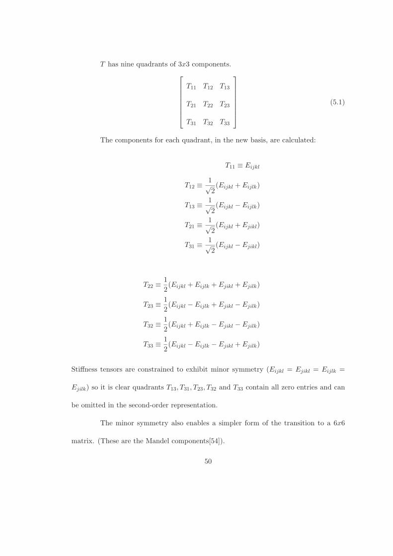
T has nine quadrants of 3x3 components.
"
#
#
#
#
#
#
$
T11 T12 T13
T21 T22 T23
T31 T32 T33
%
&
&
&
&
&
&
'
(5.1)
The components for each quadrant, in the new basis, are calculated:
T11 & Eijkl
T12 &1)2(Eijkl + Eijlk)
T13 &1)2(Eijkl % Eijlk)
T21 &1)2(Eijkl + Ejikl)
T31 &1)2(Eijkl % Ejikl)
T22 &1
2(Eijkl + Eijlk + Ejikl + Ejilk)
T23 &1
2(Eijkl % Eijlk + Ejikl % Ejilk)
T32 &1
2(Eijkl + Eijlk % Ejikl % Ejilk)
T33 &1
2(Eijkl % Eijlk % Ejikl + Ejilk)
Sti!ness tensors are constrained to exhibit minor symmetry (Eijkl = Ejikl = Eijlk =
Ejilk) so it is clear quadrants T13, T31, T23, T32 and T33 contain all zero entries and can
be omitted in the second-order representation.
The minor symmetry also enables a simpler form of the transition to a 6x6
matrix. (These are the Mandel components[54]).
50

Given a 3x3x3x3 tensor Eijkl with indices E1111 through E3333, an equiva-
lent 6x6 matrix M is made by substituting entries from Eijkl and multiplying by the
appropriate constants:
M =
,
-
-
-
-
-
-
-
-
-
-
-
-
-
-
-
-
-
-
-
.
E1111 E1122 E1133
)2E1112
)2E1123
)2E1131
E2211 E2222 E2233
)2E2212
)2E2223
)2E2231
E3311 E3322 E3333
)2E3312
)2E3323
)2E3331
)2E1211
)2E1222
)2E1233 2E1212 2E1223 2E1231
)2E2311
)2E2322
)2E2333 2E2312 2E2323 2E2331
)2E3111
)2E3122
)2E3133 2E3112 2E3123 2E3131
/
0
0
0
0
0
0
0
0
0
0
0
0
0
0
0
0
0
0
0
1
(5.2)
A second-order symmetric tensor S such as stress or strain, in the same basis
will be the transpose of
2
S11 S22 S33
)2S12
)2S23
)2S31
3
(5.3)
The transpose makes the form of the constitutive equation for solid mechanics appear
as in chapter 3.
51

Chapter 6
Decomposition of Fourth-Order Sti!ness
Tensors for Visualization
A major focus of current research in civil, mechanical and other branches of
engineering is modeling and simulating behaviors of solids and structures made up of
various materials (soils, concrete, steel, etc.). Realistic models of solids allow engineers
to design safer machines and structures. The fourth-order 3D sti!ness tensor plays a
pivotal role in such modeling and simulations. The sti!ness tensor represents the rela-
tionship between increments of stress and increments of strain. Sti!ness changes state
during plastic deformation and failure, so visualization is an important tool for providing
(1) insight into material behavior and (2) visual verification of a model. Visualization
of fourth-order tensors has not been explored in depth previously, as noted in chapter
4. Challenges include (1) the large number of components (3x3x3x3 for 3D), (2) loss
of major symmetry and (3) loss of positive definiteness, with possibly zero or negative
52

Table 6.1: How a sti!ness tensor can change with increasing stress.
Material Behavior Symmetry Tensor Propertieselastic symmetric positive-definiteelastic-plastic asymmetry eigenvalue magnitude reduction,
nonsingular if hardeningfailure, localized asymmetry non-positive definite, possibly sin-
gular
eigenvalues.
One goal of this work is to find a decomposition that (a) reduces the number
of components to visualize and (b) highlights the most interesting regions of a volume.
The term “interesting” is domain dependent, but the decomposition should be general
enough to be useful for many branches of engineering that model and simulate solids. We
present a decomposition of fourth-order tensors that facilitates their visualization. The
method can be applied to many solid mechanics applications, including Geomechanics.
It highlights susceptibility to failure, a feature of interest for engineers.
6.1 Sti!ness Changes
Solid materials undergo a sequence of changes under increasing loads. In gen-
eral, increasing loads beyond the elastic limit induce changes in the sti!ness tensor
described in table 6.1.
53

6.1.1 Elastic Behavior
In this dissertation, “elastic” is used synonymously with temporary deforma-
tion; the deformation reverses on removal of forces. As an example of elastic defor-
mation, imagine a paper clip: it will elastically change shape to hold a small stack
of papers, su!ering virtually no permanent deformation after the papers are removed.
Brannon notes plasticity theories typically presume that there exists some contiguous
domain of stress levels for which permanent (non-recoverable) deformation is negligible
[58]. The governing equation to be solved is
#ij = Eeijkl$kl (6.1)
Here, Ee symbolizes elastic sti!ness #ij symbolizes stress increments and $kl symbolizes
strain increments. Elastic sti!ness tensors are both major symmetric (Eeijkl = Ee
klij)
and minor symmetric (Eeijkl = Ee
jikl = Eeijlk = Ee
jilk), as well as positive definite.
6.1.2 Elastic-Plastic Behavior
We use the word “plastic” synonymously with permanent deformation. When
a paper clip is deformed by a large amount, only a portion of the deformation is recovered
upon removal of the force. As discussed by Brannon [12], this familiar observation is
generalized in plasticity theory with the strain increment $ as a sum of a recoverable
elastic part plus a permanent plastic part. The onset of plastic deformation is extremely
important. With permanent deformation, a machine part may need to be repaired or
replaced. A building may become unsafe. The soil may no longer be able to support a
54

bridge adequately. The governing equation for elastic-plastic behavior is
#ij = Eepijkl$kl (6.2)
where Eep symbolizes elastic-plastic sti!ness.
Materials modeled as elastic-plastic are characterized by a yield function,
F (#ij), a function of stress.(See chapter 3 for more details). The yield criterion, which
delineates points at which stress causes elastic-plastic deformation versus pure elastic
deformation, is defined at
F (#ij) = 0 (6.3)
The yield surface is the zero isosurface as described by equation 6.3. Stress states causing
F (#ij) < 0 correspond to elasticity. Stress states causing F (#ij) ( 0 are attainable only
via plastic loading[12], a type of loading that causes some permanent deformation.
6.1.3 Hardening and Softening
Classical equations of plasticity theory model the stress increment as a fourth-
order elastic-plastic sti!ness tensor acting on the total strain increment [12]. The
elastic-plastic sti!ness tensor’s formulation is a function of the elastic sti!ness, yield
function F (#ij), plastic flow function G(#ij), and other internal model variables. A
“non-hardening” material has a fixed yield surface. Brannon notes that during plastic
loading of non-hardening materials, the stress increment is constrained to move tangent
to the yield surface, and the elastic-plastic sti!ness tensor is a positive-semi-definite
rank-one projection operator. It essentially removes the part of the elastic stress incre-
55

ment that points outside the yield surface[58].
For a hardening material, the yield surface can expand outward, as shown in
figure 6.1. Then, increasingly higher levels of stress are required to continue plastic
loading. In this case, the elastic-plastic sti!ness tensor is positive definite and invertible
(non-singular).
Figure 6.1: Yield surfaces (meridian plane) with various types of hardening or softening.p: volumetric stress (pressure), q: deviatoric (distortional) stress. Figure source: [35]
For a softening material, the yield surface contracts in the neighborhood of
the stress, so diminishing stresses are needed to continue plastic loading Brannon notes
that in this case, the elastic-plastic sti!ness tensor can become non-positive definite[58].
Depending on the nature of the loading, softening can lead to an instability in the
material response that is characterized by an intense localization (increased strain rate
in a defined region) of the deformation in narrow bands[73].
56

6.1.4 Localized Failure
With enough bending force, a paper clip will deform permanently and even-
tually break. According to early literature, a solid (in this case a clip) is said to “fail
locally” when the sti!ness tensor is singular. Here, “locally” means that the solid breaks
or liquefies at a set of points, or region, inside the domain [53, 61, 64]. Singularity is
identified by one or more zero eigenvalues. Later literature identified localized failure at
the point of loss of positive definiteness [61]. A primary goal of this visualization work is
to filter the field of evolving tangent sti!ness tensors to identify regions near or beyond
the localization threshold and to visualize the corresponding modes of susceptibility to
failure.
6.2 Related Work on Decomposition
In 2007, Basser and Pajevic [6] applied eigen-decomposition to a fourth-order
symmetric covariance tensor for feature detection in DT-MRI, producing a set of six
second-order eigentensors. The authors also noted that the mathematical underpinnings
of these eigentensors came from Lord Kelvin’s work to identify modes of deformation
in linear elastic solids. Eigentensors have also been used to classify symmetries in
anisotropic solids such as crystals[72].
While Basser and Pajevic applied the decomposition to fully symmetric positive-
definite covariance tensors, these ideas motivated our own research with respect to more
general fourth-order sti!ness tensors. It seemed plausible that the loss of sti!ness would
57

cause a significantly lowered eigenvalue, and I posited that the eigentensor associated
with this eigenvalue might have some relation to the mode of stress that would cause
large deformation.
Maier and Hueckel gave the criterion for a solid breaking (bifurcation or failure)
as a singular sti!ness tensor[53]. This criterion is significant because a singular sti!ness
must have at least one zero eigenvalue. Neilsen and Schreyer were the first to use
an eigen-decomposition procedure to determine the deformation mode associated with
the bifurcation[61]. Their criterion for bifurcation was the loss of positive definiteness,
which occurs before singularity. First, they performed a decomposition to obtain the
symmetric part of the sti!ness,
sym(E) =1
2(E + ET ) (6.4)
since E is positive definite if and only if sym(E) is positive definite. Then they followed
with eigen-decomposition on the symmetric part of the sti!ness tensor. When positive
definiteness was lost, they used the eigentensor of the zero eigenvalue of sym(E) as
the mode of bifurcation. Note that the eigentensor of sym(E) is not necessarily an
eigentensor of E itself, unless E is symmetric.
6.3 Our Approach
We should be able to detect susceptibility to failure and nature of the sti!ness’
vulnerability, in terms of stress. In our approach, we perform a polar decomposition
on the sti!ness, followed by eigen-decomposition on the polar “stretch”. The two step
58

decomposition was proposed by Brannon[58]. Polar decomposition is a technique to
separate a matrix into two component matrices,
E = R S (6.5)
where S is a pure stretch (symmetric positive-semidefinite matrix), and R is a pure
rotation (orthonormal matrix) [29, 22, 31, 30, 86, 24]. Polar decomposition is known in
plasticity and mechanics literature, but our use of it for analyzing the sti!ness tensor is
new. Nielsen and Schreyer [61] showed that eigen-decomposition on the symmetric part
of the sti!ness tensor produced the critical deformation mode at failure. Like Nielsen and
Schreyer, we can detect the loss of sti!ness when a significantly low eigenvalue occurs.
With polar decomposition, however, Brannon posits that the eigentensor associated with
a significantly low eigenvalue represents the stress mode that will produce the greatest
deformation. The polar decomposition also appears to tell us about the changing flow
direction of permanently deforming material.
6.3.1 Method Constraints
Brannon’s decomposition recovers facets of the original modelers’ composition.
However, it also leads to some constraints on the range of models where the method
can be applied. Our method can be applied to sti!ness tensors exhibiting the following
properties:
• Fourth-order tensors with minor symmetry : The method relies on the second-
order tensors (stress and strain increments) being symmetric, which constrains
59

the fourth-order sti!ness tensor to exhibit minor symmetry.
• Elastic-plastic material models: Our method is applicable to general elastic-plastic
models, and it can also be applied to any material behavior where the sti!ness
tensor changes as the loading progresses such as pressure sensitive elasticity or
damage.
• Small deformation theory : According to Brannon, “Small deformation” refers
to problems with only small displacement gradients. This means that the sti!-
ness tensors are cast with respect to the reference configuration such that any
changes in sti!ness associated with rigid material rotation are eliminated from
consideration[58].
• Absence of elastic-plastic coupling : With elastic-plastic coupling, plastic flow can
a!ect the elastic properties[12]. and is an additional source of non-associativity[33].
6.3.2 Method Details
Our decomposition is composed of the following steps:
1. Unroll the 3 " 3 " 3 " 3 tensor into a 6 " 6 matrix using Mandel components
(See chapter 5 for details). The 81-component sti!ness tensor has 36 independent
components, preserved in the new basis.
2. Perform a polar decomposition on the 6"6 matrix, producing two 6"6 matrices:
the rotation part and the stretch part.
60

3. Perform an eigen-decomposition on the stretch part of the polar decomposition,
yielding 6 eigenvectors and 6 real eigenvalues.
4. Compose an eigenvector into a symmetric 3"3 eigentensor if it has a significantly
lower single eigenvalue, reversing the unrolling.
5. Visualize the second-order eigentensor with a glyph that shows its structure and
also shows significant features such as eigenvalue or mode.
Continuous visualization (integrated across the volume) of the second-order tensor field
is also possible.
6.3.2.1 Unrolling
Unrolling from tensor to matrix requires placing the constants in specific ma-
trix entries and multiplying by constants as shown in equation 6.6.
M =
,
-
-
-
-
-
-
-
-
-
-
-
-
-
-
-
-
-
-
-
.
E1111 E1122 E1133
)2E1112
)2E1123
)2E1131
E2211 E2222 E2233
)2E2212
)2E2223
)2E2231
E3311 E3322 E3333
)2E3312
)2E3323
)2E3331
)2E1211
)2E1222
)2E1233 2E1212 2E1223 2E1231
)2E2311
)2E2322
)2E2333 2E2312 2E2323 2E2331
)2E3111
)2E3122
)2E3133 2E3112 2E3123 2E3131
/
0
0
0
0
0
0
0
0
0
0
0
0
0
0
0
0
0
0
0
1
(6.6)
This casts the fourth-order tensor in Mandel form[54]. Mandel components provide
an orthonormal basis[74]. In addition, they form an isomorphism between the double
61

contraction (Eijkl $kl) and the equivalent single contraction (Mij $j)[6]. The details of
the basis are covered in chapter 5.
6.3.2.2 Polar Stretch and Mode of Vulnerability
Eigen-decomposition is performed on the symmetric stretch matrix S from the
polar decomposition. This can be done using the lapack library [3]. We analyze the
eigen-decomposition of S to find the eigenvector associated with its smallest eigenvalue.
Then, we convert this first-order eigenvector Vi, i = 1 . . . 6 to a symmetric second-order
eigentensor Sij :
Sij =
"
#
#
#
#
#
#
$
V11%2V4
1%2V6
1%2V4 V2
1%2V5
1%2V6
1%2V5 V3
%
&
&
&
&
&
&
'
(6.7)
Equation 6.7 is the inverse of unrolling operation shown in chapter 5 equation 5.3.
The initial eigenvalues of a sti!ness tensor are based on the bulk modulus and shear
modulus of the material, and the initial sti!ness matrix is a pure stretch; its rotation
component is the identity. With loading forces su"cient to cause plastic deformation,
the sti!ness may change as described in section 6.1.3, and resistance to certain types of
stress increments may be reduced.
A polar decomposition of sti!ness matrix E quantifies this degradation. Loosely,
eigenvalues of S (the “stretches”) are larger than their initial values if the material has
sti!ened. If they are smaller, it has become less sti!. According to Brannon, the
62

corresponding eigentensors of S represent loading modes[58].
Suppose the stretch eigenvector associated with the smallest eigenvalue is [0,
0, 0, 1, 0, 0]T (eigenvectors are column vectors). The corresponding normalized stretch
eigentensor is:
"
#
#
#
#
#
#
$
0+
1/2 0
+
1/2 0 0
0 0 0
%
&
&
&
&
&
&
'
This is a pure shear on the X-Y plane. If the corresponding eigenvalue is 0.75 of its
initial value, then the material is 25% less resistant (sti!) to shear on the X-Y plane
than it was initially. Selecting the lowest stretch eigenvalue can therefore reveal which
regions are su!ering significant plastic loading when many di!erent types of materials
are used in a simulation. As the sti!ness matrix approaches singularity, having a robust
computation procedure, as described in section 6.4 is crucial. An eigenvalue approaching
zero is considered to be a failure mode for the material.
If E is nonsingular and has negative eigenvalues, the physical meaning of the
polar decomposition is unclear. Even if a symmetric-antisymmetric decomposition is
used instead, its meaning is still unclear. According to Brannon, the occurrence of a
negative eigenvalue in the sti!ness matrix corresponds to dynamic softening instability,
which requires di!erent di!erential equations of motion[58]. In our visualization, we use
a uniquely shaped black glyph to indicate an occurrence of a negative eigenvalue, and
interpretation of its mode of vulnerability is not possible.
One issue for visualizing eigentensors is evident in the triaxial case. The eigen-
63

tensor represents either triaxial tension or triaxial compression. For an eigenvector yj
of polar stretch Sij of sti!ness, in Mandel form, with the lowest eigenvalue, and its
eigenvalue ", both of the following are true:
Sij yj = " yj (6.8)
Sij (%yj) = " (%yj) (6.9)
Since the eigenvector multiplied by any constant satisfies the equations, the lapack
library [3] may choose either case while solving the eigen decomposition. In order to
correctly determine whether we have triaxial tension or triaxial compression, we need
to do an additional test.
This test was suggested by Rebecca Brannon[1]. If we convert the Mandel
eigenvector to its equivalent second-order symmetric eigentensor form Yij , we can test
its “direction”. It should be oriented during plastic loading such that,
(F
(#ijEe
ijkl Ykl > 0 (6.10)
Here $F$%ij
is the yield surface normal and Eeijkl is the elastic sti!ness, for the particular
integration point. If the condition in equation 6.10 is not satisfied, we multiply the
eigentensor by %1. Then, it will have the correct orientation.
6.3.2.3 Polar Rotation and Elastic-Plastic Materials
The rotation part of the polar decomposition also carries interesting informa-
tion. As we have mentioned in chapter 3, elastic-plastic materials are characterized by
64

a yield function and a plastic flow potential function.
In associated material models, the yield surface and plastic flow surface co-
incide, and the plastic strain increment “direction” is the same as the “normal” to
the yield surface[81]. Numerically, the yield surface normal is calculated as the partial
derivative of the yield function with respect to stress, $F$%ij
. In associated materials there
is no rotation component (R is the 6D identity matrix).
We conjecture that for non-associated materials, the polar rotation (in 6D)
quantifies the degree of misalignment of the yield surface normal( $F$%ij
) and the plastic
flow direction( $G$%ij
). In other words, we conjecture that applying the polar rotation to
the yield surface normal produces the plastic flow direction to a good approximation.
We confirmed this conjecture for some material models, as shown in the results section
6.6. However, it requires further empirical and theoretical evaluation.
6.4 Polar Decomposition Algorithm
One issue for polar decomposition on sti!ness is that the matrix is not amenable
to traditional numerical methods. During plastic yielding, the sti!ness matrix can
become positive semi-definite and therefore is not invertible; traditional methods use
inversion. Moreover, the accompanying zero eigenvalue means that the polar decompo-
sition is not unique. Although a general polar decomposition algorithm exists[31], we
had already embarked on the creation of a new one that was much simpler and equally
accurate for a single, near-zero or zero eigenvalue[58].
65

6.4.1 Simple Polar Decomposition for Positive-Definite Matrices
Van Gelder proposed the new algorithm[58], which I implemented, adding code
to increase accuracy and debugging as I went along. The algorithm starts by finding
the polar stretch S of sti!ness matrix E and checking the number of near-zero or zero
eigenvalues. We define D, and its relationship to the polar stretch S:
D = ET E = ST S = S2 (6.11)
D = T J T T (6.12)
T’s columns are eigenvectors and J is diagonal with sorted eigenvalues.
S = T)
J T T where)
J is nonnegative (6.13)
S =1
2(S + ST ), improving accuracy (6.14)
If there are no zero or near-zero eigenvalues, the rotation R can be calculated
with an inversion:
R = E S!1 (6.15)
The correctness of the algorithm follows from D’s properties of being symmetric and
positive semi-definite, and T being orthogonal so that TT = T!1.
6.4.2 Algorithm for a Zero or Near-Zero Eigenvalue
In the case of a zero or near-zero eigenvalue, the general idea is to use Gram-
Schmidt completion to find the zero eigenvalue’s column vector so that it is orthogonal
66

to the others in T, necessary for a rotation matrix. We can use the same method as
shown in section 6.4.1 for calculating initial stretch S, J and initial T. We start by
defining a matrix variable C in terms of T. The goal is to find C and use C to calculate
rotation R. The steps of the algorithm are as follows:
C & R T (6.16)
B = E T = R S T = R(T)
J T T )T = C)
J (6.17)
Next, we calculate column vectors Cj from column vectors Bj , except the one
corresponding to the zero eigenvalue:
Cj = Bj /)
J jj for j = 2, . . . , n (6.18)
Finally, we use Gram-Schmidt projection to get the final column of C
C1 = Gram-Schmidt completion of 6D orthonormal basis (6.19)
R = C T T (6.20)
S = sym4
R!1 E5
(6.21)
The last step, enforcing symmetry, increases the accuracy of the stretch matrix.
6.4.3 Additional Details
When D has a zero eigenvalue there can be either a negative or positive de-
terminant for D. We choose a positive determinant, as if the matrix had been positive
definite. If the determinant is negative, we enforce this constraint by multiplying the
67

first column of T by %1. (An eigenvector multiplied by any constant is also an eigen-
vector of a given matrix). This is done before the calculation B = E T in equation
6.17.
Additionally, to avoid dividing by zero in equation 6.18, we first make the zero
eigenvalue of the diagonal matrix J into a 1. In our implementation, we know that
it corresponds to the first column of C since the eigenvalues were previously sorted in
ascending order.
Finally, we perform Gram-Schmidt on columns 2, . . . , n and normalize them
to make the orthogonalization more accurate. C1 is then replaced with 1 for the first
value and zero for the rest as a normalized “guess” vector before completing the Gram-
Schmidt projection.
6.5 Analysis of Rotation Representation
In order to understand and analyze the rotation portion of the polar decom-
position of the elastic-plastic sti!ness, we need to look at how elastic-plastic sti!ness is
calculated.
In classical non-associative plasticity (without elastic-plastic coupling), the
elastic-plastic sti!ness tensor calculation is of the form
Eepijkl = Ee
ijkl % (PijQkl)/) (6.22)
Ee is the symmetric, positive-definite elastic sti!ness and PijQkl is a dyad, and ) is a
scalar. This is the form found in the earthquake engineering simulator, OpenSees[62].
68

The dyad P # Q which has rank two (equal to that of Pij) even though P # Q is
a fourth-order tensor. P # Q has a single non-zero eigenvalue and its eigentensor is
equivalent to the first operand (P) times a scalar. Subtracting a dyad from symmetric
fourth-order tensor Ee changes the stretch in at least one of its second-order eigentensors
and potentially induces a rotation.
In the analysis, we show that the polar rotation rotates P into Q. However,
we note that the rotation from P to Q is not unique.
6.5.1 Origin of Dyad Components
This section covers the origin of P and Q and ) from equation 6.22. The
section can be skipped if the details of solid mechanics modeling are not of interest to
the reader.
In addition to the yield function F (#) and plastic potential function G(#), the
simulator calculates the derivative of F and G and returns second-order tensors we will
call A and B. These are respectively the yield surface “normal” and plastic potential
surface “normal” described in section 6.3.2.3.
A =(F
(#ij(6.23)
where F is the yield function.
B =(G
(#ij(6.24)
where G is the plastic potential function.
69

Next, A and B are each contracted with the elastic sti!ness Ee.
Pij = EeijklAkl (6.25)
Qkl = BijEeijkl (6.26)
These are P and Q for our dyad P # Q. The symbol ) is a scalar of the form
) = H + AijEeijklBkl (6.27)
Here, H is the so-called ensemble hardening modulus (a scalar)[12].
For the remainder of the discussion, we will use equivalent 6D vectors with
Mandel components for the equivalent symmetric second-order matrices (as shown in
equation 5.3) and 6D matrices with Mandel components for fourth-order tensors with
minor symmetry as shown in equation 6.6. The use of matrices and vectors allows the
analysis to follow actual numerical implementation used in testing.
6.5.2 Justification for Rotation
This analysis came from Brannon. Let F = P # Q/). Substituting F into
equation 6.22 gives
Eep = Ee % F (6.28)
Doing a polar decomposition on Ee % Eep is the same as doing a polar decomposition
of F . F is not positive definite, so we have to use pseudo-inverses where an inverse is
needed. Let F T denote the transpose of F . Then
F T F = ((Q # P )(P # Q))/)2 = (pq/))2(Q # Q) (6.29)
70

FF T = ((P # Q)(Q # P ))/)2 = (pq/))2(P # P ) (6.30)
P normalized to unit length is P , and Q normalized to unit length is Q. P is calculated
Pp where p =
+
(Pi Pi), the magnitude. The scalar q likewise represents the magnitude
of Q. Because of the nature of dyads, the fourth-order right and left polar stretch
tensors are
U = (pq/))(Q # Q) (6.31)
V = (pq/))(P # P ) (6.32)
We seek a rotation R such that
F = R S (6.33)
F = V R (6.34)
Writing these using F = P # Q/) and equation 6.31 gives
(P # Q)/) = (pq/))R(Q # Q) (6.35)
(P # Q)/) = (pq/))(P # P )R (6.36)
Dividing both sides by (pq/)) gives
P # Q = R(Q # Q) (6.37)
P # Q = (P # P )R (6.38)
Finally, we note that
R(Q # Q) = (R : Q) # Q (6.39)
71

and
(P # P )R = P # (P : R). (6.40)
Therefore, by omitting to take the same outer product on both sides of the equations:
P = R : Q (6.41)
Q = P : R (6.42)
This shows that the rotation tensor from pseudo polar decomposition of Ee%Eep defines
the rotation of Q into P .
6.6 Results
We want to be able to test whether equation 6.41 and equation 6.42 hold for
the material models in our earthquake engineering simulator. We start by normalizing
P and Q from the simulator and call them P1 and Q1.
P1 =P
*P*)(6.43)
Q1 =Q
*Q*(6.44)
Next we rotate P1 and Q1 using the polar rotation matrix R of the elastic-plastic
sti!ness.
P2 = R : Q1 (6.45)
Q2 = P1 : R (6.46)
We want to test how close the rotated matrices come to satisfying P2 = P1 and Q2 = Q1.
72

6.6.1 Testing Methods
I compared the second-order tensor P1 of equation 6.43 with P2 of equation
6.45 by two methods. The first method computes the Euclidean distance between the
two tensors:
difference =6
!
(Pij1 % Pij2)2 (6.47)
Since both tensors were normalized (magnitude of one) and the column vectors of R
were normalized, the maximum possible di!erence was two.
The second method uses the definition of dot product
P1 · P2 = |P1||P2| cos ! (6.48)
The di!erence between tensors is defined as the angle ! between P1 and P2. If P1 and
P2 are the same, ! is zero and the maximum di!erence is 2* radians. Although this
definition was originally applied to vectors, we apply it here to second-order tensors. I
applied the same tests to Q1 of equation 6.44 and Q2 of equation 6.46.
6.6.2 Tests of Material Models
We took measurements from similar simulations with three material models:
an associated material (Drucker-Prager), a non-associated material (Drucker-Prager
with a Von-Mises yield surface), and a non-associated material with elastic-plastic
coupling(Dafalias-Manzari).
In the case of Drucker-Prager, A and B were equivalent and all of the rotations
were the identity matrix. A and B represent the yield surface “normal” and plastic
73

potential surface “normal” as described in section 6.3.2.3. If A is equivalent to B, then
P1 is equivalent to Q1. This was exactly what we expected for an associated material and
clearly equations 6.45 and 6.46 were satisfied with an identity matrix for the rotation.
The Euclidean test resulted in all zero values and the values for ! were all near zero
within numerical precision.
For the first non-associated material (Drucker-Prager with a Von-Mises yield
surface), the results were quite interesting. Figures 6.2 and 6.3 show results for step
124, the final step in the simulation.
Figure 6.2: Non-Associated Model,! between rotated Q and P
The histograms show two distinct buckets, at zero and 1.26 radians. However,
if we show only the cases where the rotation is not the identity, the zero bucket alone
remains. (See figure 6.4).
The significance for this is that in the calculation of sti!ness, below a certain
threshold, only the elastic sti!ness is used. Non-associativity still holds in P and Q, but
they are not used in the calculation of sti!ness. The sti!ness is elastic (fully symmetric
74

Figure 6.3: Non-Associated Model,! between rotated P and Q
Figure 6.4: Non-Associated Model, ! di!erence between rotated P and Q for non-identity rotations
and positive definite) and its polar rotation is the identity. Therefore, when the sti!ness
is elastic and the material is non-associated, the polar rotation does not reflect the
rotation between P and Q.
Finally, we see a full range of values for Dafalias-Manzari, with two peaks
(figure 6.5). We have shown the data set using Euclidean di!erence rather than !
because 0-100% can be more easily mapped to a 0-2.0 range. We expected the main
bucket to have shifted right of zero at least 10% (mapping to 0.2 in the given range)
75

due to elastic-plastic coupling. Instead we see 2 peaks, near 0.4 and at 2.0, and a full
spectrum of values. Thus, there are additional factors that remove this model from the
class that can get a meaningful rotation from the polar decomposition of sti!ness.
Figure 6.5: Dafalias-Manzari model,Euclidean di!erence between rotated Q and P
76

Chapter 7
Visualization of Second-Order, 3D,
Non-Positive-Definite Symmetric
Tensors
Chapter 4 details previous work with glyph, hyperstreamline and topology
approaches for visualizing second-order symmetric tensor fields. Most fall short in ad-
dressing the needs of solid mechanics engineering because they do not find features
of interest to the domain, or are limited to positive-definite or 2D tensors. In this
chapter, we start with the features of interest and then present some new visualization
approaches, experiments and results.
77

7.1 Stress and Strain Tensor Features
Tensor fields resulting from Geomechanics computations are mostly related to
the state of stress (sij) and strain ($ij). Both are symmetric, and non-positive definite.
Stress is characterized by five basic modes, and a stress tensor may represent a pure
mode or some combination of them. (Strain can likewise be characterized). The modes
are:
1. spherical tension (three equal positive eigenvalues).
2. spherical compression (three equal negative eigenvalues).
3. triaxial compression (two equal eigenvalues with the distinct eigenvalue more com-
pressive than the repeated eigenvalues).
4. triaxial tension (two equal eigenvalues with the distinct eigenvalue less compressive
than the repeated eigenvalues).
5. pure shear (one zero eigenvalue, with the others equal and opposite in sign).
An isotropic stress (with three equal eigenvalues) corresponds to pressure which
is equal from all directions. This case is similar to isotropy for DT-MRI [79] but can rep-
resent either compression (negative eigenvalues) or tension(positive eigenvalues). Triax-
ial tension or compression produces an axisymmetric stress (symmetric about one axis)
and it is characterized by two equal eigenvalues. A state of pure shear stress is where
one eigenvalue is zero and the other two are equal and opposite in sign.
78

7.1.1 Stresses in Geomaterial Solids
Stress tensors are of particular importance in solid mechanics, and Geomechan-
ics as well, as they are useful as failure indicators. A large majority of Geomechanics
theories deal with elastic-plastic behavior and failure of solids. Failure is based in stress
space, putting a strong emphasis on understanding of stress tensor field. According to
Jeremic, Geomechanics uses stress tensors to understand the behavior of soil and objects
embedded in the soil as support for structural elements above. For example, concrete
piles support buildings, bridges, or water tanks. The main features of interest are:
• Zones with positive stress (tension), particularly in piles. Tension results in crack-
ing concrete.
• Zones with large shear stresses. In soil this can cause large shear deformations
and shear failure.
• Zones of sign changes. A sudden switch from compressive to tensile behavior
results in tensile failure.
Concrete and soils can withstand large compressive forces but fail under tension or
in shear [39, 40, 36, 41]. These critical features are usually present at the interface
between sti! concrete piles and soft surrounding soil, but they can occur anywhere in
the solids[60].
79

7.2 Reynolds Glyphs
We used Reynolds glyphs to visualize the mode of stress that a solid is vulner-
able to after it reaches the yield point. This was a test for the decomposition method
represented in chapter 6. We hoped the visualization would show (a) regions that had
become less sti! and (b) the mode of stress that would cause maximum deformation in
those regions.
Reynolds glyphs visually depict characteristic modes of stress or strain [6].
The formula for a point on the surface of the second-order Reynolds glyph, using tensor
notation from chapter 2 is:
c = ni #ij nj (7.1)
Here, i, j range over 1, 2, 3 and 1, 2, 3 are Cartesian axes. n represents a 3D normalized
vector of the direction cosine perpendicular to the plane of interest. In other words,
each vector n represents a point on a unit sphere centered at (0, 0, 0).
Reynolds glyphs, coupled with color mapping, can clearly distinguish the five
modes of stress. For instance, isotropic tension would be represented as a red sphere, and
isotropic compression would be a blue sphere. For triaxial tension or triaxial compres-
sion, formula 7.1 produces an axisymmetric Reynolds glyph. The axis of symmetry is
aligned with the eigenvector of stress corresponding to the distinct eigenvalue as shown
in figure 7.1b. The disk shape in figure is similar to planar anisotropy for DT-MRI
second-order tensors, also characterized by two equal eigenvalues [79].
80

Spherical Tension Triaxial Compression Pure Shear
(a) (b) (c)
Figure 7.1: Reynolds Glyph representations of modes of stress. Cool colors (blue andcyan) represent negative values, hot colors (red and yellow) represent positive. The X,Y, and Z axes are red, green, and blue respectively.
Pure shear produces a glyph such as the one in figure 7.1c. The distinct
butterfly appearance of pure shear is caused by equal magnitude and opposite values
across orthogonal directions on a single plane. This is the plane where shearing occurs;
in this example it is the X % Y plane.
7.2.1 Graphical Issue
One graphical issue for Reynolds glyph arises when the scalar value c stretch-
ing the vector n is negative. The direction of the vector is reversed, and calculating
the correct surface normal is more di"cult. However, since the underlying tensor is
symmetric, we can assume the glyph will be likewise symmetric. We can draw the point
and calculate the surface normal without reversing the direction of n since both n and
-n are on the surface of the glyph. We simply color them both with the magnitude of c.
81

7.2.2 Associated Scalar Color Fields
As noted in chapter 6, under su"cient stress a solid can yield, experiencing per-
manent deformation. When this happens, one or more eigenvalues reduce in magnitude.
To find regions losing sti!ness, we use the lowest eigenvalue from the decomposition of
sti!ness detailed in chapter 6. Coloring by minimum eigenvalue highlights regions where
significant loss of sti!ness and permanent deformation have occurred.
We also use the Lode angle !, a stress invariant, to classify the mode of devia-
toric stress[51, 56]. The original use for Lode angle was in the formulation of yield func-
tions for isotropic solid material models, as well as others based on stress eigenvalues[12].
(More details on the yield function can be found in chapter 6.) The Lode angle is for-
mulated:
! =1
3sin!1[
7J3
2
87 3
J2
83
2
] (7.2)
J2 is the deviatoric stress invariant
J2 =1
2* S *2 (7.3)
where S is the deviatoric part of the stress tensor #ij .
Sij = #ij %1
3#kk&ij (7.4)
Here &ij is the Kronecker delta, the 3x3 identity matrix. J3 is the determinant of Sij .
Figure 7.2 shows a yield surface (zero isosurface of the yield function) for a typical
geomaterial, and a slice of the surface. The coordinate system is the orthogonal eigen-
82

vectors (“stress space”) rather than Cartesian. The slice illustrates the continuous and
reflective nature of the classification scheme despite ordering of eigenvalues.
Figure 7.2: Yield Surface (Stress-Space Isosurface) for an isotropic material and Lodeangles for single slice. Image source: [12] TXE stands for triaxial extension, TXC istriaxial compression, SHR is shear, BXC is biaxial compression, and BXE is biaxialextension..
Figure 7.3: Lode Angle Color Scale and Glyphs
Figure 7.3 shows a rainbow color mapping of Lode angle, and the glyph shapes associated
with the scalar values.
83

7.2.3 Experiment
We tested our technique on two simple experiments from Geomechanics. Both
experiments consisted of 224 finite elements, each with 8 integration points on an irreg-
ular grid; a total of 1792 points for the volume. The experiments were run on OpenSees,
a finite-element simulator for performance of structural and geotechnical systems sub-
jected to earthquakes [62]. Data for the visualization was gathered during the runs,
which took 10.5–12 minutes on an Intel 6600 2.4 Ghz dual core desktop with 2.0 gi-
gabytes of RAM. The visualization runs at 1–4 frames per second, depending on the
window size. Excerpts are shown in the figures. The software and experiment scripts
are available from the authors and will soon be available through the VEES project
website [57].
The experiments started with self-weight analysis of the soil, compressing along
%Z, for 25 time steps. This is a common practice when studying soil behavior. The
initial compression from the soil’s own weight induces deformation and may also change
the sti!ness, depending on the model. The second part of the experiment was two
point loads on the top of the volume. The loads included a small component along
%Z (0.9659 kiloNewtons) and a large lateral component (1294 kiloNewtons). This part
of the experiment ran for another 100 steps. Figure 7.4 shows the volume colored by
displacement (Euclidean distance from initial position) on the last time step. The black
arrows point to where the loads were applied along +X. In Figure 7.5a, 7.5b, 7.6a
and 7.6b, we drew glyphs for each integration point in the volume, and the glyph size
84

Figure 7.4: Deformation (Euclidean distance), time step 124. Arrows indicate locationand direction of applied point loads. Drucker-Prager material model.
was scaled by the size of the encapsulating finite element. These eigentensor glyphs
were colored by the lowest eigenvalue and scaled across all time steps to give an overall
idea of softening or hardening. In the case where the solid had not started permanent
deformation (yielded), we drew spheres to indicate the elastic, isotropic material model.
We used a black cube for the case of a negative eigenvalue in the sti!ness tensor so the
engineers could quickly identify singularity and the inability of the simulator to produce
the mode of the instability.
The first soil material was Drucker-Prager. The material simply fails under
tension, but it remains unchanged under compression (a “non-hardening” material).
There were no changes in material sti!ness during the self-weight steps. The material
lost sti!ness during the point load stress regime in the neighborhoods around and be-
neath the point loads, as shown in figure 7.5a. The mode of stress the solid became
vulnerable to was similar to applied stress in the regions with loss of sti!ness; triaxial
compression in front of the point loads along the X axis, shear along the sides of the
85

point loads and between them, and triaxial tension behind the applied loads. The user
can quickly pick out these modes with Lode angle coloring (see figure 7.5b). Blue and
cyan highlight the compression in front of the point loads, yellow trailing behind indi-
cates tension, and green indicates shear. In this simple example, glyphs show a clear
change in orientation and indicate principal stress directions (eigenvectors).
(a) (b)Lowest eigenvalue scalar coloring. Top view (from +Z), Lode angle scalar coloring.
Figure 7.5: Drucker-Prager material model, time step 124.
The second simulated material was Dafalias and Manzari’s plasticity sand
model [15]. The model’s sti!ness is pressure-dependent and non-associated. In or-
der to make the experiment repeatable we used the material constants given in the
article, with the exception of the initial void ratio (e0). This material softens when it is
denser (with smaller void ratios). Since we wanted to test our method’s ability to detect
softening, we reduced e0 to 0.65. In this experiment, self-weight induced hardening. The
86

greatest hardening occurred at the bottom of the volume, where the finite-element nodes
were fixed and experiencing the greatest load from above. At first, sti!ness increased
with the depth of the volume, as expected with self-weight loading. With continued
self-weight, loss of sti!ness occurred in the volume we saw some integration points
with negative eigenvalues. As the experiment continued, loss of sti!ness occurred along
the side boundaries of the volume, but there was frequent change between elastic and
elastic-plastic states. It was di"cult to correlate the stress to the behavior because of
the changing yield surface and non-associativity. However, we did notice loss of sti!ness
on the top surface near the applied point loads late in the experiment (Figure 7.6a).
(a) (b)Lowest eigenvalue log scalar coloring. Lode angle scalar coloring.
Figure 7.6: Dafalias-Manzari material model, time step 124.
87

7.3 Plane-In-A-Box Glyph
The motivation for our new glyph, plane-in-a-box, is to visualize high shear
(both orientation and magnitude) as well as discriminate tension versus compression.
The plane-in-a-box glyph is quite similar in appearance to tensor ellipsoids for the case
when there is strong planar anisotropy. This glyph presents the same amount of relevant
information as tensor ellipsoids using a simpler representation.
(a) (b)Single plane in enclosing box. Side view of a volume of plane-in-the-box glyphs.
Figure 7.7: Plane-in-a-box glyph.
The idea of plane-in-a-box is to create a plane with limited extent at each sample point.
The size of the planar glyph is limited by a box whose edges are half the distance to
each of the neighboring points. If the point is on a face of the volume, we simply extend
it out a distance to half the distance of the neighboring interior point. Occlusion is
88

reduced by scaling the planar glyphs while maintaining the general orientation. We
opted for this simpler glyph since we are primarily interested in regions characterized
by high shear. Pure shear exists on a single plane, and both triaxial tension and triaxial
compression have a planar component. Thus, mapping the tensors to planar glyphs
is quite natural. The plane spans the eigenvectors associated with the largest (major)
eigenvalues, and the plane normal implies the eigenvector direction associated with the
smallest (minor) eigenvalue. The plane itself can also be colored or filtered according
to scalar parameters of interest. We explore the use of four scalars in the hope that
they will help us find features of interest, namely: high shear, tension, and changes from
compression to tension.
7.3.1 Data Structures and Algorithms
The plane-in-a-box glyph has two requirements. First, the sampled points
must lay on a mesh, preferably a grid (although the grid need not be regular). In either
case some connectivity among sample points is necessary to establish the locations of
the edges of the box. For rectilinear data, we simply sort the points by the Z, Y, and
X axes during preprocessing. Once the points are read in, we can deduce connectivity
of neighboring points by checking the next and previous row, column, and slice.
We came to realize that finite element results do not necessarily lie on straight
lines, as shown in 7.13. There are pie-shaped elements and variable sizes. For these
data sets we take advantage any type of regularity that exist. In our case, slices on the
Z plane were regular distances apart. We run Delaunay triangulation on the remainder
89

to get connectivity. For both cases, connectivity is stored in an adjacency list.
7.3.1.1 Creating the Box and Finding Edge-Plane Intersections
The first step in creating glyphs is to create the box whose edges will limit the
plane. By iterating through the linked list of rectilinear neighbors, we can determine the
minimum and maximum X,Y, and Z distances to neighbors. We set box edges at half
the distance to the neighbors and can even reduce the scale of the distance, if desired.
Figure 7.8: A box is formed around a point, based on the location of neighboring points.
For Delaunay neighbors we use a slightly simpler technique. We check the
distance to each neighbor and select the one that is closest. We halve the distance
and set that as the bounding distance along axes for which we have no rectilinear
distances. This gives us good guarantees against polygon overlap although it may not
be proportional to distance between points in all three directions.
Once we have the distances, we set the corners of the box using a lookup table
which matches minimum or maximum X,Y, and Z to each box corner.
The next step is to create the plane, finding which edges of the box it intersects
90

and where on the edge the intersection occurs. We have a plane defined using point-
normal form, where the normal is the eigenvector corresponding to the minor eigenvalue.
We convert it to general form
Ax + By + Cz + D = 0 (7.5)
where A, B, and C are the X, Y, and Z components of the normal respectively. With
the sample point at x0, y0, z0,
D = (%1 + norm[X] + x0) % (norm[Y ] + y0) % (norm[Z] + z0) (7.6)
Then, for each edge of the box, we use Bourke’s algorithm [9] to find the
intersection by extending the edge until it touches the plane.
Pintersect = t(P2 % P1) (7.7)
where P1 and P2 are the points forming an edge of the box as shown in figure 7.9.
Substituting t(P2 % P1) into our implicit plane equation yields
A(x1 + t(x2 % x1)) + B(y1 + t(y2 % y1)) + C(z1 + t(z2 % z1)) + D = 0 (7.8)
and solving for t gives
t =Ax1 + By1 + Cz1 + D
A(x1 % x2) + B(y1 % y2) + C(z1 % z2)(7.9)
91

Figure 7.9: Intersection of plane and box edge. P0 is the Gauss point.
The intersection occurs at P1 + t(P2 % P1). Once we have an intersection, if it lies on
the edge between P1 and P2, we update the box’s edge index and store the intersection
point in its marching cubes array.
In summary, we begin by creating a box which is limited by half the distance its
neighbors. We calculate A, B, C, and D for our plane, based on the point location and
its normal. Then we check each edge of the box to see if the plane intersects it, saving
the intersection point Pintersect and building an edge intersection case index. Finally,
the edge intersection index is cross–referenced to a Marching Cubes index [52].
7.3.1.2 Marching Cubes for Simple Planes on an Irregular Grid
After extracting the intersections of the planes with the edges of the cell con-
taining the tensor, the next step is the creation of the triangles that make up the plane.
Our algorithm uses a variation on the well-known Marching Cubes [52].
Our algorithm di!ers in two ways:
92

Figure 7.10: Marching Cubes cases. (256 total with symmetry). Source: [52].
1. The index is built on edge intersections rather than a boolean for above or below
an isovalue.
2. The box is composed of variable-sized quadrilaterals rather than a cube.
We deal with the first item by creating a mapping from each of the 256 march-
ing cubes case indices to its corresponding edge index and save them in our reverse
lookup table. More specifically, we iterate through each marching cubes triangle case
array, building an active edge index. Then we make a hash table with the edge index as
the key and the marching cubes index as the value, for fast retrieval. Figure 7.11 shows
an example mapping. The hash table is used just before the call to marching cubes.
Below is the pseudo code for the algorithm.
int plane_in_a_box(int i)
{
calculate A, B, C, D
make_box( i, box, plane_in_a_box_scale );
for( j = 0; j < 12; j++ ) /* box edges */
{
calculate t
93

Figure 7.11: Mapping from plane-edge intersection to Marching Cubes index
calculate edge-plane intersection
if ( intersection is within edge )
{
/* copy edge intersection:
2 out of 3 dimensions identical */
mc_edges[j][X] = box[cube_edges[j][1]][X];
mc_edges[j][Y] = box[cube_edges[j][1]][Y];
mc_edges[j][Z] = box[cube_edges[j][1]][Z];
mc_edges[j][edge_dim[j]] =
touch_plane[edge_dim[j]];
/* update edge case */
index = index + CASE_INDEX[j];
}
}/* for each box edge */
/* cross reference MC index */
index = get_value( MC_hash, index );
marching_cube( i, index, mc_edges );
}
Despite our box forming a hexahedron instead of a regular cube, we have
found that marching cubes works quite well. Two facts help us. First, when we form
the box around a sample point on the plane, we guarantee the box will enclose the
plane. Second, because we build the case using a plane that spreads to the limits of
94

the box, we never see the ambiguous marching cubes indices. Simply, since we build a
continuous surface, we do not have holes. However, two other types of ambiguous cases
Figure 7.12: Sliding the box (brown to blue) to resolve case of edge lying in the plane.
can occur. One case is where an edge of the box lies in the plane. For such a plane, there
are an infinite number of intersection points for the edge and the plane. Furthermore,
three edges will claim intersection for each corner of the edge in the plane. In this case,
a proper marching cubes index cannot be formed. The second ambiguity is where the
plane intersects an edge at a box corner. As with the previous case, three edges will
claim intersection for each corner of the edge in the plane. The simple solution is to shift
the box a tiny amount along one axis and recalculate. We found this solution e!ective;
we selected the first of multiple possible case indices, and shifted the box back before
building the plane’s triangles.
We predicted that we would see just a few di!erent marching cubes cases as
the point would sit in the middle of the box. This soon proved wrong as the sample
point may lie almost anywhere within a skewed box.
95

7.3.2 Associated Scalar Color Fields
Stress features of interest for Geomechanics include tension, shear, sudden
changes from compression to tension. We test four scalar measures for color mapping,
opacity and filtering the plane glyphs. We provides several di!erent scalar measures to
aid exploration of a data set, and filtering mechanisms to home in on areas of interest
in the volume. Three of the scalar measures come from Seismology and the fourth from
tensor topology.
The scalar features are (i) signed isotropy (with both linear and log scaling),
which is equivalent to spherical tension and compression from solid mechanics (ii) Seis-
mic Double Couple (DC), which is equivalent to pure shear from solid mechanics (iii)
Seismic Compensated Linear Vector Dipole which is equivalent to triaxial tension or
triaxial compression from solid mechanics. (iv) Eigen di!erence [84].
7.3.3 Seismic Moment Tensors
Seismologists use a seismic moment tensor Mij for a general representation of
the seismic source [19]. Seismic moment tensors, like stress tensors, are symmetric and
non-positive-definite. However, they di!er in a couple of very important ways.
Seismic moment tensors or acoustic emission moment tensors are created from
a measured event such as an earthquake or cracking solid. Sound waves are emitted
at the event and can be measured. Thus, one major di!erence is that moment tensors
represent a strictly elastodynamic source [43]. Second, in Geomechanics, a stress tensor
relates to forces applied on the exterior surface of a volume. Moment tensors instead
96

relate to forces that cause displacement across an internal surface, where the internal
surface represents a buried fault [2].
Dreger et al. note that Mij is commonly decomposed into isotropic, double
couple (DC) and compensated linear vector dipole (CLVD) components, where each
of the components of the moment tensor decomposition is represented as a percent-
age of the total [19, 46, 43]. The same numerical features select for spherical ten-
sion/compression, shear, and triaxial tension/compression respectively. At the time
this research was performed, however, we were not yet aware of the basic categories of
mechanical stress, as described in section 7.1.
7.3.3.1 Isotropic and Deviatoric Components
Finding these scalar components starts with finding the eigenvectors and eigen-
values of Mij = T J T T . A diagonalized moment tensor J can be further decomposed
into isotropic and deviatoric parts. A purely isotropic tensor is characterized by three
equal eigenvalues. The isotropy in a moment tensor represents a change in volume. Pure
isotropy in a moment tensor is comparable to an ideal explosion (positive eigenvalues)
or implosion (negative eigenvalues) [20]. The equivalent for stress is spherical tension
or compression. The isotropic portion is the identity matrix scaled by the mean of the
three eigenvalues. The deviatoric component is the remainder of the original matrix
after the isotropic component has been removed.
Below is the mathematical notation for the isotropic and deviatoric components
of matrix J , where the trace (tr) is the sum of the diagonal elements and m$i is Jii %
97

tr(J)/3. Here, m$1 has the smallest absolute magnitude and m$
3 the largest.
J =
"
#
#
#
#
#
#
$
tr(J)3 0 0
0 tr(J)3 0
0 0 tr(J)3
%
&
&
&
&
&
&
'
+
"
#
#
#
#
#
#
$
m$1 0 0
0 m$2 0
0 0 m$3
%
&
&
&
&
&
&
'
(7.10)
7.3.3.2 Two Vector Dipoles
Moment tensor elements represent dipoles. A dipole is composed of two equal
and opposite vectors laying along an axis orthogonal to both of them. The physical
meaning is the direction and angle of tectonic plate movement along opposite sides of
a fault. According to Dreger, double couple (DC) consists of two linear vector dipoles
of equal magnitude but opposite sign, resolving shear motion on faults. The shear
is oriented 45 degrees to the principal eigenvectors of Mij [19]. In mechanical terms,
if the force in the double couple exceeds a material’s threshold, a shearing event will
occur [20], or displacement along the fault plane (parallel to the largest stress). In a
pure DC event, the eigenvalues are proportional to 1, 0,%1 [43]. In this section we use
DC and pure shear interchangeably.
Compensated linear vector dipole (CLVD) refers to when “a change in volume
is compensated by particle motion in the plane parallel to the largest stress” [20].
This may be a mechanism for deep earthquakes [46]. CLVD is modeled by eigenval-
ues proportional to %2, 1, 1, reflecting particle motion. Figure 4.9 shows the failure
mechanisms associated with pure isotropy, DC, and CLVD.
The contribution of DC and CLVD to the deviatoric component of a moment
98

tensor can be calculated as follows: For components of the diagonalized moment tensor
without isotropy, m$1, m
$2, m
$3 such that
|m$3| ( |m$
2| ( |m$1| (7.11)
F = %|m$
1||m$
3|(7.12)
F is the ratio of the smallest to largest absolutes of the eigenvalues and we expect a value
of 0.0 for pure DC and 0.5 for pure CLVD. Note that F does not distinguish triaxial com-
pression (m$i , (1, 1,%2)) and triaxial tension (eigenvalues m$
i , (%1,%1, 2)). However,
one could examine the sign of m$1, and create a scalar that gives similar information to
the Lode angle.
Assuming the deviatoric is a result of only DC and CLVD,
mdeviatoric =
m$3(1 % 2F )
"
#
#
#
#
#
#
$
0 0 0
0 %1 0
0 0 1
%
&
&
&
&
&
&
'
+ m$3F
"
#
#
#
#
#
#
$
%1 0 0
0 %1 0
0 0 2
%
&
&
&
&
&
&
'
(7.13)
For scalar features there are two quantities:
DC = m$3(1 % 2F ) (7.14)
CLV D = m$3F (7.15)
99

Following Anderson and Finck [4, 20], percentage of deviatoric that is CLVD can be
calculated:
2m$3F
|2m$3F | + |m$
3(1 % 2F )|(7.16)
The CLVD is doubled so there can be a range of 0.0 % 1.0 instead of 0.0 % 0.5. We use
the estimate * 2F * for culling and coloring glyphs for simplicity.
Zheng, et al. categorized double degenerate points in a second-order symmetric
tensor field by first sorting eigenvalues by absolute magnitude: |"1| ( |"2| ( |"3|.
Planar degenerate points had |"1| = |"2| ( |"3| and linear degenerate points had
|"1| ( |"2| = |"3|. [84]. They proposed a scalar K as:
K = 2"2 % ("1 + "3) (7.17)
where K is a positive value for planar degenerate tensors (identical major and medium
eigenvalues), and a negative value for linear degenerate tensors (identical medium and
minor eigenvalues). We were curious to see how the scalar would operate on our tensor
field.
7.3.3.3 Scalar Calculation and Meaning
We built an application with a menu for selecting a feature for coloring the
planes and a feature for setting plane opacity.
Since the two features, DC and CLVD, can be expressed as percentiles, they
are automatically scaled from 0 to 1. For isotropy and eigen di!erence, we set the zero
valued features (the midpoint) at 0.5. We scaled cool colors (blue) below, from 0.5
100

to 0 for negative values and hot colors (red) for positive values scaled up from 0.5 to
1. Opacity can provide some filtering e!ect as the lowest values are fully transparent.
Medium to high values appear more solid and their geometry is highlighted, similar to
volume rendering, and we mapped scalars to opacity with the same scale.
The application also has sliders for selecting a range of values for features. For
example, a user can select strictly positive isotropy combined with high CLVD. Such
combinations allow users to search for domain-specific indicators. The aforementioned,
for example, can signify a crack when the data set is composed of moment tensors
from acoustic emissions [20]. With thresholding, the shape of regions are also clearly
delimited. Essentially, the user can create isosurface and iso-volume-like selections.
However, the surface is not smooth, being composed of individually oriented planes.
Finally, the application can show the inverse of a selected feature range, providing
greater flexibility.
7.3.3.4 User Interaction
Rather than thresholding over the entire volume, a user may wish to explore
from points of interest on outwards. We provide a pointer that the user can move around
the volume to select various seed points. Then, on each iteration, neighboring planes get
painted. This gives an animation e!ect of oriented planes growing out of the seed point.
Thresholding constraints may also be applied, as desired. For this type of interaction,
we built two data structures that save state between animation frames. One is a draw
list where each entry refers to a sample point in the volume. This is initialized to all
101

zeros to indicate no planes should be drawn; only non-zero entries have their planes
drawn during an iteration. The second is a queue that holds the sample point numbers
to be added to the draw list on the next iteration. In addition, the point adjacency
is stored in an adjacency list, implemented as an array of linked lists. The algorithm
proceeds as a simple breadth first traversal. At first glance, the extra complexity may
seem unnecessary; after all, for regular data we can simply use the stride of the length,
width, and slice of the rectilinear sorted data. However, in many cases, Geomechanics
data is not regular. Gauss points across finite elements are not lined up along X and
Y, as shown in figure 7.13. We would still like to explore a region from a selected seed
point, and breadth first traversal of the mesh works well for this.
After initialization with the user’s selected seed points, we take each point
from the queue, add it to the draw list, and check its linked list of neighbors. Here
again, we depend on having neighbor connectivity available. We do a check three things
before we consider adding a new point to the next iteration’s queue. The sample point
must meet all of the user’s constraints, and neither the current draw list nor the current
queue may already contain it.
The data structures and process are very similar to Gibson’s Chainmail algo-
rithm [23]. The Chainmail algorithm enables fast deformation of volumetric objects,
composed of objects such as nodes and points from Finite Element analysis. The anal-
ogy is that points and nodes move as if joined by a chain link mesh. If a node is moved
beyond a constraint, neighboring nodes will also move. Similarly, on each iteration of our
algorithm, new candidates are queued breadth-first and previously selected candidates
102

are tested against the constraints.
7.3.4 Data Meaning
The particular data sets used in this paper are related to two applied Geome-
chanics problems. The first data set represents a finite sized model with two point
loads on top, the Boussinesq problem (i.e. [50]). The problem is simple enough that
the results are known in advance and represents an excellent verification procedure. In
addition, symmetry planes in the model can be used for verification of numerical and
visualization procedures.
The second data set is from a dynamic, seismic bridge simulation. It represents
a stress field from one time step of an elastic-plastic, dynamic simulation of a soil–
foundation–structure (SFS) bridge system [8, 7]. This data set involves large ratios
of stresses between sti! concrete in columns of the main structure, and the soft soil
beneath. In addition, the main characteristics of the stress fields are not known in
advance as we use simulations to gain a better understanding of the behavior of the
SFS system and the interactions of its components during seismic events.
7.3.5 Data Representation
The volume of the bridge–soil system is built from finite elements. Each ele-
ment has a hull of vertex nodes that may be shared with neighboring elements. The
shape of an element need not be rectilinear. Within each element are gauss points.
That is, the Gaussian method is used to locate points that produce the most accurate
103

Mesh of Finite Elements Single 8-Node Element (Gauss points are data locations)
Figure 7.13: Finite Element Data Set
integration.
As the simulation progresses, nodes move, inducing stress at the gauss points.
Hence, the stress tensor field consists of the induced stresses at these gauss points.
7.3.6 Results
We tested our application using two data sets, each of which was a single time
step in a Geomechanics simulation. Both data sets consisted of a field of stress tensors
for geomechanical soils and solids, as described in section 7.3.5.
The first was the Boussinesq point load, where force was applied at two points
on the top of the volume. The second was a bridge supported by two piles in soil. In
the simulation, force was applied to one side of the bridge, followed by seismic shaking.
104

7.3.6.1 Boussinesq Point Load
Figure 7.14a shows isotropy in the double point load data set. Linear scaling
of the color map highlights the compressive and tensile forces at the points they were
applied.
The eigenvalues at these points were extremely high, so the linear scale caused
the rest of the volume to appear to have zero isotropy evenly throughout. However,
when we change to a log scale and scale the opacity as well, the variation from negative
to positive is strongly emphasized (Figure 7.14b). Here, advantage of the isotropy
scalar is clear. It shows not only the type of stress, but also its degree. There is high
tension (positive isotropy) below one point load, high compression below the other, and
a mixture on the surface.
(a) (b)Linear rainbow scale color, arrows show applied loads Log scale color and opacity.
Figure 7.14: Boussinesq dual point load, isotropy color map
105

All glyphs Thresholding, 0.50 - 0.715 Thresholding, 0.975 -1.00 (pure shear)
(a) (b) (c)
Figure 7.15: Double point load, DC color map (CLVD is the dual and has the sameappearance but with blue instead of red)
Figures 7.15a, b, and c show the coloring for the double couple feature (1.0% * F *).
The range of colors tells us that the anisotropy types range from pure shear (DC) to
midway between pure shear and triaxial tension or compression(CLVD). We omitted
CLVD since it is calculated as the dual of DC and would appear as blue–green color
mapping instead of green–red. It is clear regions with the pure shear feature are distinct
from regions with high isotropic tension or compression.
In Figures 7.15b and c, we see the results of DC thresholding. Both figures show greater
than 50% similarity to the DC feature, but the first figure has a color representing lower
similarity overall. We found it interesting that using a lower threshold selected the very
noisy data around the points where stress was applied. The region most closely matching
a DC feature was where we expected the shear to occur – on the plane between where
106

the two opposing forces were applied. Combinations of constraints on several types
of features may lead to better understanding of stress within a volume, in addition to
a scalar representing magnitude of anisotropy. For example, isotropic stress is largest
at the point where the loads are applied (Figure 7.14). The DC feature is strongest
on the plane between the two opposite loads, a very di!erent region of the volume
(Figure 7.15c). Positive isotropy in combination with anisotropic behavior might lead
to fracture.
7.3.6.2 Bridge Pile Data Set
Figures 7.17a and b show the entire volume for bridge supports embedded in
soil. The piles penetrate halfway down onto the soil. In the simulation, the applied
force, shown as the yellow arrow in figure 7.17a, pushed the bridge support to the right.
The expected behavior is is that the left side of the pile will be under tension and the
right side under compression, as shown in figure 7.16. The eigen di!erence coloring
Figure 7.16: Yellow arrow shows applied pushover force. Red arrows show resultingtension, and blue arrows show compression.
107

highlights the changes in stress with red and blue coloring above the surface and within
the piles. The sharp red-blue contrast along the upper neck of the piles and in the
bridge emphasizes that type of stress is flipping from linear to planar. In figure 7.17b,
within the neck of the piles, there is a red line indicating high DC. Therefore, there is
pure shear occurring at the location of the flip.
Eigen di!erence (log scale) DC coloring
Yellow arrow shows applied force.
(a) (b)
Figure 7.17: Bridge Data Set.
There is a circular appearance in the planes’ orientation at the center of the volume. This
is attributable to boundary e!ects in the simulation and represents a very important
finding as it tells us that the model needs to be enlarged in order to more realistically
simulate the half-space. Figure 7.18 shows thresholding by isotropy. This is an example
108

of using the inverse of a threshold range, eliminating everything in the range from 0.25-
0.75. The figure is colored by log scale isotropy and shows ranges of 0.0-0.25 representing
compression and 0.75-1.0, representing tension. The bridge pile on the right has a color
change from red to blue just above where the pile enters the soil, indicating that the
stress has switched from tension to compression. This is one of the critical features
in Geomechanics that can result in tensile failure. The isotropy figure also shows a
Figure 7.18: Bridge data set, log scaled isotropy, 0.0-0.25 and 0.75-1.0
shadowing e!ect. Shadowing comes from an analogy between the applied force and
light, where a supporting member may absorb or block the force. Its shadow is an area
under less stress. The shadowing is indeed interesting as it directly and visually conveys
information about an important physical behavior, namely the back bridge support will
be shadowed by the front bridge support, and savings can be made in reinforcement
109

steel for shadowed bending.
Figure 7.18 also presents a visual proof that the model can and needs to be
extended in the horizontal direction in order to simulate the half space more realisti-
cally. Ideally, the simulation would be su"ciently large that the boundaries would be
una!ected by the applied force. However, this is always a tradeo! with computation
cost and even with this smaller model we can get meaningful results.
7.3.7 Conclusions
One of the goals of plane-in-a-box was to find planes of shear. This was ac-
complished in the case of pure shear or DC, where there is one zero eigenvalue and
shearing occurs in the plane of the two eigenvectors with non-zero eigenvalues. Here,
using the zero eigenvalue’s eigenvector as the plane normal makes perfect sense. In the
case of CLVD, there is not a single shearing plane. Maximum shear occurs at 45 # from
the plane of eigenvectors with equal eigenvalues. In this case it might make more sense
to visualize the planar part (the plane of eigenvectors with equal eigenvalues) or use a
di!erent type of glyph than a plane. No planar glyph makes sense for pure isotropy.
Isotropy turned out to be the most useful feature among those we tried. Along
with thresholding, it highlighted information about the materials’ physical behavior
under stress. The scalar K was the least useful as it could really only apply to positive
definite data. Both triaxial compression and triaxial tension are by the definition planar
degenerate, yet have K values of opposite sign; both should have a positive K value.
110

7.4 Continuous Visualization
Continuous visualization such as hyperstreamlines have been used successfully
for fluid dynamics data, DT-MRI data, and 2D stress tensor fields. In this section, we
explore approaches to visualizing stress, strain or sti!ness eigenmode tensor fields using
a continuous visualization.
7.4.1 Interpolating to a Regular Mesh
One issue for continuous visualization of these tensor fields is that the finite
element method is often used for simulation. Finite elements, as shown in figure 7.13,
are irregularly shaped and can simulate discrete material types. Sti!ness may not cross
element boundaries, and we do not want to assume a continuity that may not exist.
Therefore, interpolation needs to respect boundaries of the finite elements.
The basic algorithm is:
For each point location within the volume {
Find finite element enclosing point location
Get tensor at each Gauss integration point within element,
and its Cartesian location.
for each tensor component {
Run Shepard’s interpolation algorithm on component.
}
}
This algorithm runs in O(G*E) where G is the number of regular grid points and E is the
number of finite elements. We used a simple caching method to improve performance;
we tested whether the current point location is in the same element as previous, before
111

doing a brute force search.
7.4.2 Creating an Eigenvector Field
There are two issues for 3D hyperstreamlines. First, one must choose one of
three hyperstreamlines, major, medium or minor. Secondly, Zheng et al. note it is gen-
erally impossible to sort the eigenvalues in a consistent and continuous fashion and hence
the hyperstreamlines, while continuous, may exhibit sudden changes in directions [84].
We propose that the significant eigenvector for a point in the volume of solid
mechanics data depends on the type of stress at the point, and should be chosen relative
to maximum shear. We can use the Lode angle ! to ascertain the anisotropic stress type.
This is calculated directly from the tensor, and the angle ! ranges from %30# (triaxial
compression) to +30# (triaxial tension), with 0# indicating pure shear. This is shown in
figure 7.2. If the eigenvalues are sorted in ascending order (but not by absolute value),
it is very easy to select the eigenvector of interest.
Triaxial Compression Pure Shear
(a) (b)
Figure 7.19: Reynolds glyphs, and the maximum shear directions for each stress mode,and the eigenvector selected based on Lode angle.
112

The algorithm has four simple cases:
• (! - %10)
Triaxial compression, sorted eigenvalues (-2,+1,+1)
Use first eigenvector, associated with smallest eigenvalue
• (! > %10 && ! - +10)
Pure shear, sorted eigenvalues (-1, 0, +1)
Use second eigenvector, associated with middle eigenvalue
• (! > +10)
Triaxial tension, sorted eigenvalues (-1,-1,2)
Use third eigenvector, associated with largest eigenvalue
• Isotropic stress (three equal eigenvalues)
All possible sets of three orthogonal vectors are eigenvectors of the tensor. None is
significant. Possible approaches include halting the hyperstreamline, or continue
it on its previous trajectory with a shape or color change indicating isotropy.
The reason these eigenvectors are of interest is that shear occurs in a consistent direction
relative to the eigenvector associated with the selected eigenvalue. Pure shear occurs in
a plane orthogonal to the selected eigenvector. Shear associated with triaxial tension
or triaxial compression occurs 45# o! from the selected eigenvector. Figure 7.19 shows
113

Reynolds Tensor Glyphs Eigenvector Arrow Glyphs
(a) (b)
Figure 7.20: Drucker-Prager Sti!ness Eigenmode field, colored by Lode angle.
Reynolds glyphs with maximum shear drawn in black. Eigenvectors selected by the
Lode angle criterion are shown. Figure 7.20 shows an example of such an eigenvector
field using eigenmode from Drucker-Prager sti!ness.
7.4.3 Future Work
The name of the proposed visualization is “Necklaces”. The “string” of the
necklace is a hyperstreamline, and the “beads” on the necklace are glyphs that show
stress type and maximum shear orientation, when viewed from any direction (see figure
7.21). Spherical tension and compression will be represented as spheres (no shear), pure
shear as planes with lines indicating the directions of maximum shear. Triaxial tension
and compression will have cones oriented along the eigenvector associated with the
largest absolute value. The surface of the cone will be along the direction of maximum
114

shear (45# o! from eigenvector with the largest absolute eigenvalue). Using parameters,
it will be possible to change continuously between the three shapes. Filtering can be
used to find the stress types of interest.
Figure 7.21: Glyph and tensor line “necklace”.
There are two advantages in this approach:
1. The “beads” along the necklace reduce the di"culty of following tensor lines’
orientation. For example, perspective viewing will change the size of the beads as
they recede from the user’s viewpoint.
2. In regions where stresses have similar orientation, a pattern will emerge along
the orientation of maximum shear. The pattern is due to the e!ects of reifica-
tion (Gestalt psychology), where an object is perceived as having more spatial
information than is present in the original stimulus.
115

This technique will be both visually appealing and useful. It will show one of the
principal stresses, direction of maximum shear, and stress type. Scalar color mapping
can show one additional attribute (such as magnitude of maximum shear or isotropy)
and be used for filtering.
116
Chapter 8
Documentation of VEES Software
8.1 Introduction
This section of the thesis provides documentation of the software, VEES[59](Visualizer
for the Earthquake Engineering System), developed to support the research. It includes
a user guide and architecture documentation.
We planned to address visualization of finite element solid mechanics data by
providing a general application to allow exploration of a simulation domain. Addition-
ally, we planned to provide a means for the user to focus on a specific element within
a domain and new techniques to show the critical details at the location. The hope is
that we will come to understand what is important to observe at both levels and so help
future users to more easily find the “good and the bad stu!”.
The main theme, for usability, is Shneiderman’s well known three level ap-
proach from information visualization: overview, zoom and filter, and details-on-demand
117

Figure 8.1: VEES visualization environment.
[71].
VEES plugs into the object-oriented OpenSees[62] finite element simulator.
OpenSees contains natural hierarchies of Finite Element Types such as volume elements
(Bricks), beams, and trusses and Materials representing soil, concrete, steel, etc. The
simulator immediately provides all geometry as well as associated scalar and tensor
data. The theme for the VEES architecture is the Strategy design pattern[21] (using
an interchangeable family of algorithms, for visualization).
118

8.2 User Guide
8.2.1 Linux Setup and Getting Started
It is necessary to have GLUT and GLUI 2.2-2.2 libraries installed in addition
to the modified version of OpenSees and its required libraries.
OpenSees can be run as a command line or by using tcl scripts. Modify your
own tcl scripts by adding the command, vees The vees command does not get loaded
into OpenSees until after the model is declared, e.g.
model BasicBuilder -ndm 3 -ndf 3
Calling vees should then give you the graphical user interface, but to see your
mesh, call vees after creating your nodes and elements. Note: when vees closes it will
also close OpenSees.exe (a bug!)
Execute OpenSees to start. When your script reaches the vees command it
will open a window and 2 floating menus.
The last section of this chapter contains an example script.
8.2.2 Using VEES
In any of the vees display windows, you can interact by placing the mouse in
the display window and using the following keyboard commands:
• [x] rotate about x axis
• [y] rotate about y axis
• [z] rotate about z axis
119

• [+] zoom in
• [-] zoom out
• [r] reset to original orientation
Clicking an eight node brick will show the selected element in the upper right
hand Element window.
Clicking an integration point on the element window will show details in the
Integration Point window.
8.2.3 Main Window
In the rendering control window you can choose from a drop down menu of
drawing methods.
Figure 8.2: VEES render mode controls.
Select one of the draw functions from the drop down menu. You can select
from several coloring schemes at the bottom of the main window. Each is scaled into
into a 0 to 1 range, where 0 is blue, 0.5 is green, 1 is red.
120

Element Type assigns each element type a unique random color.
Displacement is the Euclidean length of the displacement vector, i.e.+
9
(v[i] + v[i])
from each degree of freedom i up to the number of dimensions of the node (2 or 3).
Gauss Points are compatible with stress color functions only.
Sti!ness is compatible with sti!ness color functions only.
8.2.4 Filtering
There are two types of filters to explore the data:
• By value: you can limit the upper and lower value using the Max Color and Min
Color spinners, and also invert the range (show everything outside the selected
range)
• By element type: check the box for the element type you would like to hide.
8.2.5 Color Map Range Adjustment
At the bottom left, there is a widget set for color maps. You can select the
color map from the drop down list. The range for the color map is set to the (absolute)
maximum for the current time step. If the values for the time step are all very small
(absolute value between 0 and 1.0) the the color map range maximum is set to 1.0.
You can adjust the color map range by clicking on the text area, using the
backspace key to remove old digits and then typing in new ones. Sometimes it sticks a
little, just click another part of the interface and click back to make it work.
121

Figure 8.3: Select coloring scheme, adjust range and select linear or log scale.
Log scale is useful if the color map range covers several orders of magnitude,
such as for mean stress.
8.2.6 Element Window
There are two ways to select an element to view in the element window.
1. Click on the element in main window. (Note that you can only click surface
elements. If you need an interior element you will have to filter first).
2. Type the element number in the Select Element text box in the Render Controls
widget.
You can then click one of the element’s integration points to view in the Inte-
gration Point Window. The selected point will be highlighted in red.
8.2.7 Integration Point Window
This windows shows Reynolds glyphs for tensor data. There are keyboard
commands to view stress and various aspects of sti!ness.
To view the stress tensor, type G.
122

Figure 8.4: Element Viewer. Selected integration point highlighted in red.
To view the sti!ness tensor, type 7.
There are several view types of the eigentensors of sti!ness. The default is the
eigen decomposition of the polar stretch of sti!ness.
Type 8 to view the eigentensors on the non-decomposed sti!ness.
Type S to change to eigentensors of the symmetric part of sti!ness.
Type 9 to switch back to eigentensors of the polar stretch.
The numbers 0-5 display glyphs of the 6 eigentensors for the selected decompo-
sition type. Type 0 to see the eigentensor with the lowest eigenvalue. The eigentensors
are ordered from lowest eigenvalue to highest.
123

8.2.8 Capturing Images and Data for Post-Processing
I have added an OpenSees recorder command that records all node data (de-
grees of freedom, etc.) and stress, strain, and sti!ness for many elements and materials.
The command is
recorder domain <-file $filename>
Specifying the file name is optional. The default file names will be domain1,
domain2, etc. Be careful, the files can be quite large for the 3D soil materials.
The files can then be reloaded using the widget shown in figure8.2.8.
Figure 8.5: Widget for replaying times steps.
You can load a specific time step by entering the step number in the text area
under the load button and clicking Load. To move to the next time step, click the >
button. Use the < button to load the previous step.
To run through many time steps as a movie, enter the first time step in the
text area below the Load button and the last time step in the text area labeled End
Step. Then click the ! button to run forward, or " to run backwards.
I find it useful to load the last time step, set the color map ranges, and then
run through the time steps as a movie.
Save the images click the Save Image checkbox before loading time steps. It
124

is also possible to save sti!ness, stress, polar rotation, and the eigentensor associated
with the lowest eigenvalue by clicking the checkboxes. The tensors are interpolated
(component by component) to a regular grid.
8.3 Architecture
VEES acts as a plug-in to OpenSees. OpenSees is an object oriented C++
Finite Element simulator with Tcl wrappers. The data types organized in natural
hierarchy of elements such as beams or soil volume elements, as well as material models
for concrete, soil, steel, etc. A subset of the hierarchy is shown in figure 8.3. The
container for these is an object called the Domain. VEES has access to the Domain, its
Figure 8.6: OpenSees Domain class, its component Elements, and their componentmaterials.
components, and their data, as shown in the UML diagram (figure 8.3.1. It is organized
using several well-known design patterns, and some of the pattern applications are novel.
OpenSees contains multiple data sets we would like to visualize (stress, strain, sti!ness,
deformation), and we would like to be able to visualize each data set in multiple ways.
125

8.3.1 Model-View-Controller
The model-view-controller is a pattern for user interface design[47]. The idea
is to have separate objects for the application (the Model), its screen presentation (the
View), and the Controller which defines reaction to user input. Its purpose is to facilitate
multiple views of the same data set. We followed this pattern closely. The Model is the
OpenSees Domain, which holds instances of all nodes and Finite Elements, as well as
their data.
Figure 8.7: UML diagram of VEES.
The main window is an instance of GlutWin, which uses the GLUT window-
126

ing library and GLUI widget library. It has four subwindows as shown in figure 8.1.
Each subwindow had a VisWin instance which encapsulates a Viewer and a Camera,
and shared access to the Domain. The VisWin acts as a graphic Controller, handling
lighting, centering, projection, picking, rotation, zoom, and requests to filter the data
shown. Its Viewer is responsible for extracting data from the Domain and drawing it.
The simple hierarchy of Viewers is shown in figure 8.3.1. You can see that the View-
ers facilitate overview of all Finite Elements (DomainViewer) to full details at a single
Gauss integration point (GlyphViewer). This is evident in the user interface, as shown
in figure 8.1.
All the Viewers communicate with the GlutWin main window, but the Do-
mainViewer is the major work horse. It encapsulates arrays of DrawElement objects
and color maps, saves data to files, loads time steps and refreshes its view.
8.3.2 Strategy Pattern
The main theme for VEES is the Strategy design pattern[21], using an inter-
changable family of algorithms for visualization. We accomplished this through a single
level hierarchy of class DrawElement as shown in figure 8.3.2. The DomainViewer con-
Figure 8.8: DrawElement class hierarchy.
tains an array of each type of DrawElement, and iterates through the selected array on
127

a call to draw. This displays each finite element, as shown in the code snippet below:
ElementIter &theElements = theDomain->getElements();
while (( theElement = theElements->next() ) != NULL) {
drawMethods[theElement->getTag()]->drawElement(
theElement, color[theElement->getTag()],
ranges[currRange],drawStyle );
}
The DrawElement type, color map, and filtering range are all parameterized. The
DrawElement subclasses are self-explanatory except for HideElement, which exemplifies
the Command pattern[21].
8.3.3 Command Pattern
One filtering mechanism provided in VEES is filtering by Finite Element type,
as shown with checkboxes in figure 8.2. We want to be able to iterate through the
Figure 8.9: Substituting a HideElement instance for a DrawWireFrame instance, andsaving a reference to the old DrawWireFrame instance so we can revert back to it later.
elements and draw them, but we need a way to skip over the filtered elements. When
drawing is based on a scalar value, it is simple to check the scalar against the color map
range during iteration. But in the case filtering by Finite Element type, this will not
128

work. We use the Command pattern[21], encapsulating the request to hide the element
as an object. “Undo” means again drawing the object as it was drawn previously.
When an element type is selected for hiding, for each instance of that ele-
ment we substitute a HideElement instance. Since we want to be able to “undo” the
hiding, we need to save the old drawing object. The HideElement interface has a
setLastDrawnAs(DrawElement *) method, and a revert() method that returns the
old DrawElement.
8.3.4 Memento
We extend VEES and OpenSees to provide visualization during and or af-
ter a simulation run. Our lightweight framework leverages existing superclasses within
OpenSees while providing the necessities save time steps and reload in a series or indi-
vidually. We apply the Momento design pattern[21], serializing objects’ state so that it
can be saved in a file and restored, without breaking objects’ encapsulation.
We add two classes to OpenSees, DomainRecorder and File Channel. Domain-
Recorder is a subclass of the OpenSees Recorder. Recorders perform some action on
each commit step in a simulation, usually saving some type of data to a file.
Our DomainRecorder records the current state of the entire simulation domain
(stress, strain, sti!ness, deformation). In other words, it serializes all the components
(Elements, Materials) and their state to a file. The DomainRecorder takes advantage
an interface(MovableObject) that all components in the Domain must implement. Mov-
ableObjects must implement two methods
129

• sendSelf(int commitTag, Channel &theChannel) which serializes the object’s
state and sends it through a Channel which may represent a file, socket, datebase,
etc.
• recvSelf(int commitTag, Channel &theChannel, FEM ObjectBroker &theBroker)
which reads state from a Channel and reinstantiates the object via a Broker.
The interface was originally designed to assist with parallelization, by serializing objects
to send to other compute nodes. We use it instead to send state to file on each commit
step. The state of the entire simulation Domain is saved to file using the existing
sendSelf methods.
VEES loads Domain state in a similar fashion, using recvSelf. The graphical
user interface facilitates incrementing and decrementing time steps, or running an entire
simulation as a movie, as shown in figure 8.2.8. Each time we load a time step, the
Domain runs recvSelf on all its components. Then we propogate the update to each of
the Viewers. They reread the data from the Domain, and refresh the drawing.
8.4 OpenSees Example
#(jeremic,zhyang)@ucdavis.edu
# tcl example file using Template3Dep material
# Inelastic static analysis -- Triaxial test
#two load stages:
# stage 1: isotropic compression
130

# stage 2: triaxial shearing
#-------------------------
# create the modelbuilder
#-------------------------
model BasicBuilder -ndm 3 -ndf 3
set g 9.81
# -------------------
# build the model
# -------------------
node 1 1.0 1.0 0.0
node 2 0.0 1.0 0.0
node 3 0.0 0.0 0.0
node 4 1.0 0.0 0.0
node 5 1.0 1.0 1.0
node 6 0.0 1.0 1.0
node 7 0.0 0.0 1.0
node 8 1.0 0.0 1.0
# triaxial test boundary
fix 1 0 1 1
131

fix 2 1 1 1
fix 3 1 0 1
fix 4 0 0 1
# Linear elastic --id-Youngs--poisson--rho
nDMaterial ElasticIsotropic3D 2 70000 0.2 1.8
#Elastic-plastic model
#=================================
## Cam clay model: use force of 5
# yield surface M = 1.2
set ys "-CC 1.2"
# Potential surface M = 1.2
set ps "-CC 1.2"
#Scalar evol. law: void ratio Lamda Kappa
set ES1 "-NLp 0.65 0.19 0.06"
#Tensorial evolution law
set ET1 "-Linear 0.0"
# Number of tensor and scalar
# internal variables, and intial scalar value
set EPS "-NOD 1 -NOS 1 200.0"
#==================================
132

nDMaterial Template3Dep 1 2 -YS $ys -PS $ps -EPS $EPS -ELS1 $ES1 -ELT1 $ET1
# tag 8 nodes matID bforce1 bforce2 bforce3 rho
element Brick8N 1 5 6 7 8 1 2 3 4 1 0.0 0.0 -9.81 1.8
#stage 1
#==================
#isotropic load
set p 5.0
set np -5.0
pattern Plain 2 "Linear"
load 1 $np 0 0 -pattern 2
load 3 0 $p 0 -pattern 2
load 4 $np $p 0 -pattern 2
load 5 $np $np $np -pattern 2
load 6 $p $np $np -pattern 2
load 7 $p $p $np -pattern 2
load 8 $np $p $np -pattern 2
#Set up recorder
recorder domain
133

# NN1: number of iterations
set lf1 0.01
set NN1 500
system UmfPack
constraints Penalty 1e12 1e12
test NormDispIncr 1.0e-8 30 1
integrator LoadControl $lf1 1 $lf1 $lf1
algorithm Newton
numberer RCM
analysis Static
analyze $NN1
#stage 2
#=========================
#Axial loading
wipeAnalysis
equalDOF 5 6 3 3
equalDOF 5 7 3 3
equalDOF 5 8 3 3
remove recorders
recorder domain
134

#set previous load constant
loadConst time 0
# Before shifting to disp. control,
# apply reference load on the top
pattern Plain 3 "Linear"
load 5 0.0 0.0 $np
load 6 0.0 0.0 $np
load 7 0.0 0.0 $np
load 8 0.0 0.0 $np
load 1 $p 0 0
#Set up recorder for axial loading stage
recorder domain
set NN2 1000
set ndz -0.0001
system UmfPack
constraints Penalty 1e12 1e12
test NormDispIncr 1.0e-08 30 1
integrator DisplacementControl 5 3 $ndz 1 $ndz $ndz
algorithm Newton
135

numberer RCM
analysis Static
analyze $NN2
#visualize
vees
136

Chapter 9
Conclusion
In this dissertation, we have presented some novel approaches to visualizing
stress, strain and sti!ness tensors from solid mechanics. We have had some success in
decomposing fourth-order sti!ness tensors to facilitate their visualization, but further
research is needed. Clearly, solutions to visualizing a wider range of material models’
sti!ness will depend on the models’ formulation and meaning.
During the course of this research, a clearer picture has emerged of engineers’
needs with regards to visualizing stress tensors. Since materials frequently fail under
tension and in shear, shear planes, stress type and magnitude of stress invariants must
all be part of the solution. We have solved di!erent parts of the puzzle, and proposed
future work that we expect will be a more complete and satisfactory solution.
137

Bibliography
[1] Notes on quantifying modes of a second-order tensor.http://www.mech.utah.edu/ brannon/public/StressModeDetection.pdf, 2008.
[2] Keiiti Aki and Paul G. Richards. Quantitative Seismology Theory and Methods.W.H. Freeman and Company, 1980.
[3] E. Anderson, Z. Bai, J. Dongarra, et al. lapack: A portable linear algebra libraryfor high-performance computers. In Supercomputing ’90, pages 2–11, Washington,DC, 1990. IEEE.
[4] L. M. Anderson. A relative moment tensor inversion technique applied to seismicityinduced by mining, 2001.
[5] P. J. Basser, S. Pajevic, C. Pierpaoli, J. Duda, and A. Aldroubi. In vivo fibertractography using dt-mri data. Magnetic Resonance in Medicine, 44(4):625–632,October 2000.
[6] Peter J. Basser and Sinisa Pajevic. Spectral decomposition of a 4th-order covariancetensor: Applications to di!usion tensor mri. Signal Process., 87(2):220–236, 2007.
[7] Boris Jeremic. A brief overview of neesgrid simulation platform opensees: Appli-cation to the soil–foundation–structure interaction problems. In Maria Todorovskaand Mehmet Chelebi, editors, Proceedings of the Third United States–Japan Natu-ral Resources Workshop on Soil-Structure Interaction, Vallombrosa Center, MenloPark, California, USA, March 29-30 2004.
[8] Boris Jeremic and Matthias Preisig. Seismic soil–foundation–structure interaction:Numerical modeling issues. In ASCE Structures Congress, New York, NY, U.S.A.,April 20-24 2005.
[9] Paul D. Bourke. Intersection of a plane and a line. astron-omy.swin.edu.au/ pbourke/geometry/planeline, 1991.
[10] Allan F. Bower. Applied mechanics of solids. solidmechanics.org, September 2008.
[11] R. M. Brannon. Functional and structured tensor analysis for engineers, 2003.
138

[12] Rebecca M. Brannon. Elements of phenomenological plasticity: geometrical in-sight,computational algorithms, and applications in shock physics. In Y. Horie,editor, Shock Wave Science and Technology Reference Library: Solids I, chapter 6,pages 189–274. Springer-New York, 2007.
[13] R.M. Brannon. Functional and structured tensor analysis for engineers.www.mech.utah.edu/ brannon/public/Tensors.pdf, 2003.
[14] B. Cabral and L. Leedom. Imaging vector fields using line integral convolution.Computer Graphics (SIGGRAPH Proceedings), 27(4):263–272, 1993.
[15] Yannis F. Dafalias and Majid T. Manzari. Simple plasticity sand model accountingfor fabric change e!ects. Journal of Engineering Mechanics, 130(6):622–634, 2004.
[16] T. Delmarcelle and L. Hesselink. Visualizing second-order tensor fields with hyper-streamlines. IEEE Computer Graphics and Applications, 13(4):25–33, July 1993.
[17] T. Delmarcelle and L. Hesselink. The topology of symmetric, second-order tensorfields. In IEEE Visualization, pages 140 –147, 1994.
[18] R. R. Dickinson. A unified approach to the design of visualization software for theanalysis of field problems. In SPIE: Three-Dimensional Visualization and DisplayTechnologies, volume 1083, pages 173–180, 1989.
[19] Douglas S. Dreger, Hrvoje Tkalcic, and Malcolm Johnston. Dilational processesaccompanying earthquakes in the long valley caldera. Science, 288(5463):122–125,April 2000.
[20] Florian Finck, Jochen H. Kurz, Christian U. Grosse, and Hans Wolf-Reinhardt.Advances in moment tensor inversion for civil engineering. In International Sym-posium on Non–Destructive Testing in Civil Engineering, 2003.
[21] Erich Gamma, Riachard Helm, Ralph Johnson, and John Vlissides. Design Pat-terns: Elements of Reusable Object–Oriented Software. Professional ComputingSeries. Addison–Wesley, 1995. ISBN 0-201-63361-2.
[22] W. Gander. Algorithms for the polar decomposition. SIAM Journal on Scientificand Statistical Computing, 11:1102–1115, 1990.
[23] Sarah F. Gibson. 3D ChainMail: a fast algorithm for deforming volumetric objects.In Andy van Dam, editor, Proceedings Symposium on Interactive 3D Graphics,pages 149–154, April 1997.
[24] Gene H. Golub and Charles F. Van Loan. Matrix Computations. Johns Hopkins,third edition, 1996.
139

[25] Youssef M.A. Hashash, John I-Chiang Yao, and Donald C. Wotring. Glyph andhyperstreamline representation of stress and strain tensors and material consti-tutive response. International Journal for Numerical and Analytical Methods InGeomechanics, 27(7):603–626, 2003.
[26] James L. Helman and Lambertus Hesselink. Visualizing vector field topology influid flows. IEEE Comput. Graph. Appl., 11(3):36–46, 1991.
[27] L. Helman, J.and Hesselink. Representation and display of vector field topology influid flow data sets. Computer, 22(8):27–36, August 1989.
[28] P. Helnwein. Some remarks on the compressed matrix representation of symmetricsecond-order and fourth-order tensors. Computer Methods in Applied Mechanicsand Engineering, 190:2753–2770(18), 16 February 2001.
[29] N. J. Higham. Computing the polar decomposition – with applications. SIAMJournal on Scientific and Statistical Computing, 7:1160–1174, 1986.
[30] N. J. Higham and P. Papadimitriou. A parallel algorithm for computing the polardecomposition. Parallel Computing, 20:1161–1173, 1994.
[31] N. J. Higham and R. S. Schreiber. Fast polar decomposition of an arbitrary matrix.SIAM Journal on Scientific and Statistical Computing, 11:648–655, 1990.
[32] Mario Hlawitschka and Gerik Scheuermann. HOT- lines: Tracking lines in higherorder tensor fields. In Proceedings of Visualization ’05, pages 27–34, Minneapolis,2005.
[33] Tomasz Hueckel. Coupling of elastic and plastic deformations of bulk solids. Mec-canica, 11(4):227–235, December 1976.
[34] Mikhail Itskov. On the theory of fourth-order tensors and their applications in com-putational mechanics. Computer Methods in Applied Mechanics and Engineering,189(2):419–438(20), 1 September 2000.
[35] Boris Jeremic. Lecture notes on computational geomechan-ics (aka inelastic finite elements for pressure sensitive materials).sokocalo.engr.ucdavis.edu/ jeremic/CG/LN.pdf, 2000-2004. Lecture Notes,UC Davis.
[36] Boris Jeremic, Kenneth Runesson, and Stein Sture. Finite deformation analysis ofgeomaterials. International Journal for Numerical and Analytical Methods in Ge-omechanics including International Journal for Mechanics of Cohesive–FrictionalMaterials, 25(8):809–840, 2001.
[37] Boris Jeremic, Gerik Scheuermann, Jan Frey, Zhaohui Yang, Bernd Hamann, Ken-neth I. Joy, and Hans Hagen. Tensor visualizations in computational geomechan-ics. International Journal for Numerical and Analytical Methods in Geomechanics,26(10):925–944, 2002.
140

[38] Boris Jeremic, Gerik Scheuermann, Jan Frey, Zhaohui Yang, Bernd Hamann, Ken-neth I. Joy, and Hans Hagen. Tensor visualizations in computational geomechan-ics. International Journal for Numerical and Analytical Methods in Geomechanics,26:925–944, 2002.
[39] Boris Jeremic and Christos Xenophontos. Application of the p–version of the finiteelement method to elasto–plasticity with localization of deformation. Communica-tions in Numerical Methods in Engineering, 15:867–976, 1999.
[40] Boris Jeremic, Christos Xenophontos, and Stein Sture. Modeling of continuouslocalization of deformation. In Roger Ghanem Nick Jones, editor, Proceedings of13th Engineering Mechanics Specialty Conference, page 4 pages, Baltimore, Mary-land, June 1999. Engineering Mechanics Division of the American Society of CivilEngineers.
[41] Boris Jeremic, Zhaohui Yang, and Stein Sture. Influence of imperfections on consti-tutive behavior of geomaterials. ASCE Journal of Engineering Mechanics, 130(6),June 2004.
[42] Bruno Jobard and Wilfrid Lefer. Creating evenly-spaced streamlines of arbitrarydensity. In Eurographics Visualization in Scientific Computing Workshop, pages43–56, 1997.
[43] M.L. Jost and R. B. Herrmann. A student’s guide to and review of moment tensors.Seismological Research Letters, 60:37–57, 1989.
[44] Gordon Kindlmann. Superquadric tensor glyph. In Vissym’04, pages 147–154,2004.
[45] Gordon L. Kindlmann and David M. Weinstein. Hue-balls and lit-tensors for directvolume rendering of di!usion tensor fields. In IEEE Visualization, pages 183–189,1999.
[46] L. Knopo! and MJ Randall. Compensated linear–vector dipole–possible mechanismof deep earthquakes. J. Geophys. Res., 75:4957–4963, 1970.
[47] Glenn E. Krasner and Stephen T. Pope. A cookbook for using the model-viewcontroller user interface paradigm in smalltalk-80. J. Object Oriented Program.,1(3):26–49, 1988.
[48] R.D. Kriz, E.H. Glaessgen, and J.D. MacRae. Eigenvalue-eigenvector glyphs: Vi-sualizing zeroth, second, fourth and higher order tensors in a continuum. In Pro-ceedings of the NCSA-NIST Workshop on Modeling the Development of ResidualStresses During Thermoset Composites Curing, September 1995.
[49] David Laidlaw, Eric Ahrens, David Kremers, Matthew Avalos, Russell Jacobs, andCarol Readhead. Visualizing di!usion tensor images of the mouse spinal cord. InProceedings of Visualization ’98, pages 127–134, 1998.
141

[50] William T. Lambe and Robert V. Whitman. Soil Mechanics, SI Version. JohnWiley and Sons, 1979.
[51] W. Lode. Versuche ber den einflu der mittleren hauptspannung auf das flieen dermetalle eisen, kupfer und nickel. Zeitschrift fr Physik A Hadrons and Nuclei, 36,November 1926.
[52] W. E. Lorensen and H. E. Cline. Marching cubes: A high resolution 3D surfaceconstruction algorithm. Computer Graphics, 21(4):163–169, 1987.
[53] G. Maier and T. Hueckel. Nonassociated and coupled flow rules of elastoplastic-ity for rock-like materials. International Journal of Rock Mechanics and MiningScience, 16:77–92, 1979.
[54] J. Mandel. Generalisation de la theorie de plasticite de W. T. Koiter. InternationalJournal for Solids and Structures, 1:273–295, 1965. in French.
[55] Xiaoyang Mao, Hidenori Higashida, and Atsumi Imamiya. Fast placement of evenlyspaced streamlines on curvilinear grid surfaces. Visual Data Exploration and Anal-ysis VII, 3960(1):280–289, 2000.
[56] G. C. Nayak and O. C. Zienkiewicz. Convenient forms of stress invariants forplasticity. Journal of the Structural Division, American Society of Civil Engineers,98(ST4):949–953, 1972.
[57] Alisa Neeman. Vees: Project information.http://neesforge.nees.org/projects/vees/.
[58] Alisa Neeman, Rebecca Brannon, Boris Jeremic, Allen Van Gelder, and AlexPang. Decomposition and visualization of fourth-order elastic-plastic tensors. InIEEE/EG Symposium on Volume and Point-Based Graphics, pages 121–128, LosAngeles, CA, 2008. IEEE.
[59] Alisa Neeman, Boris Jeremic, Adam Markowitz, and Alex Pang. VEES: An XML-driven visualization and development environment. In Proceedings of the FourthNEES Annual Meeting, June 21-23 2006.
[60] Alisa Neeman, Boris Jeremic, and Alex Pang. Visualizing tensor fields in geome-chanics. In Proceedings of Visualization ’05, pages 35–42, Minneapolis, 2005.
[61] M. K. Neilsen and H. L. Schreyer. Bifurcations in elastic-plastic materials. Inter-national Journal of Solids and Structures, 30(4):521 – 544, 1993.
[62] OpenSees Development Team (Open Source Project). OpenSees: open system forearthquake engineering simulations. 1998-2005.
[63] Jean H. Prevost and Radu Popescu. Constitutive relations for soil materi-als. Electronic Journal of Geotechnical Engineering, October 1996. available athttp://139.78.66.61/ejge/.
142

[64] Egidio Rizzi, Giulio Maier, and Kaspar Willam. On failure indicators in multi–dissipative materials. International Journal of Solids and Structures, 33(20-22):3187–3214, 1996.
[65] D. Roylance. Mechanics of Materials. John Wiley & Sons, 1996.
[66] Gerik Scheuermann, Jan Frey, Hans Hagen, Bernd Hamann, B. Jeremic, and Ken-neth I. Joy. Case study: Visualization of seismic soils structure interaction sim-ulations. In Proceedings of the Joint Eurographics - IEEE TCVG Symposium onVisualization 2001, page 10 pages, Ascona, Switzerland,, May 28-30 2001.
[67] Will Schroeder, Ken Martin, and Bill Lorensen. The Visualization Toolkit: AnObject-Oriented Approach to 3D Graphics. Prentice Hall, New Jersey, 1996.
[68] T. Schultz and H.-P. Seidel. Estimating crossing fibers: A tensor decomposition ap-proach. Visualization and Computer Graphics, IEEE Transactions on, 14(6):1635–1642, Nov.-Dec. 2008.
[69] Wei Shen. Seeding strategries for hyperstreamlines. Master’s thesis, University ofCalifornia, Santa Cruz, 2004.
[70] Wei Shen and Alex Pang. Seeding strategies for hyperstreamlines. In Proceed-ings of the Seventh IASTED International Conference on Computer Graphics andImaging, 2004.
[71] Ben Shneiderman and Catherine Plaisant. Designing the User Interface: Strategiesfor E!ective Human-Computer Interaction. Addison-Wesley, 2005.
[72] S. Sutcli!e. Spectral decomposition of the elasticity tensor. Journal of AppliedMechanics–Transactions of the ASME, 59(4):762–773, 1992.
[73] L. Szabo. Shear band localization of elasto-plastic solids at finite strain. In PLAS-TICITY ’93, The Fourth Int. Symposium on Plasticity and its Current Application,Baltimore, USA, July 19-23 1993.
[74] Albert Tarantola. Elements for Physics: Quantities, Qualities, and Intrinsic The-ories. Springer-Verlag, 2006.
[75] David S. Tuch. Q–ball imaging. Magnetic Resonance in Medicine, 52(6):1358–1372,2004.
[76] Greg Turk and David Banks. Image-guided streamline placement. In SIGGRAPH’96: Proceedings of the 23rd annual conference on Computer graphics and interac-tive techniques, pages 453–460, New York, NY, USA, 1996. ACM.
[77] Vivek Verma, David Kao, and Alex Pang. Flow-guided streamline seeding strategy.In Proceedings of Visualization ’00, pages 163–170, 552, 2000.
143

[78] Eric W. Weisstein. Mathworld–a wolfram web resource. mathworld.wolfram.com.
[79] C.-F. Westin, S. Peled, H. Gudbjartsson, R. Kikinis, and F. A. Jolesz. Geometricaldi!usion measures for MRI from tensor basis analysis. In ISMRM ’97, page 1742,Vancouver Canada, April 1997.
[80] A. Wilson and R. Brannon. Exploring 2d tensor fields using stress nets. In Pro-ceedings of Visualization ’05, pages 11–18, Oct. 2005.
[81] David Muir Wood. Soil Behaviour nad Critical State Soil Mechanics. CambridgeUniversity Press, 1990.
[82] Xiaohong Ye, David Kao, and Alex Pang. Strategy for seeding 3D streamlines. InProceedings of Visualization ’05, pages 471–478, Minneapolis, 2005.
[83] Xiaoqiang Zheng and Alex Pang. Topological lines in 3D tensor fields. In Proceed-ings of Visualization ’04, pages 313–320, Austin, 2004.
[84] Xiaoqiang Zheng, Beresford Parlett, and Alex Pang. Topological lines in 3D tensorfields and discriminant hessian factorization. IEEE Transactions on Visualizationand Computer Graphics, 11(4):395–407, July/August 2005.
[85] Xiaoqiang Zheng, Beresford Parlett, and Alex Pang. Topological structures of 3Dtensor fields. In Proceedings of Visualization ’05, pages 551–558, Minneapolis, 2005.
[86] P. Zielinski and K. Zietak. The polar decomposition — properties, applicationsand algorithms. Applied Mathematics, Annals of the Polish Mathematical Society,38:23–49, 1995.
144