virtual lab - zsoil · virtual lab z soil.pc 120201 report revised 15.04.2016 by ... p.o.box 224,...

VIRTUAL LABZ Soil.PC 120201 reportrevised 15.04.2016

byR.F. Obrzud, A. Truty and K. Podles

with contribution byS. Commend and Th. Zimmermann

Zace Services Ltd, Software engineering

P.O.Box 224, CH-1028 Preverenges

Switzerland

(T) +41 21 802 46 05

(F) +41 21 802 46 06

http://www.zsoil.com,

hotline: [email protected]

since 1985

Contents

TABLE OF CONTENTS i

List of symbols viii

1 VIRTUAL LAB 1

1.1 OVERVIEW . . . . . . . . . . . . . . . . . . . . . . . . . . . . . . . . . . 1

1.2 ARCHITECTURE . . . . . . . . . . . . . . . . . . . . . . . . . . . . . . . 5

1.3 ELEMENTS . . . . . . . . . . . . . . . . . . . . . . . . . . . . . . . . . . 7

1.4 HOW TO PERFORM ... . . . . . . . . . . . . . . . . . . . . . . . . . . . . 10

1.4.1 ... PARAMETER DETERMINATION . . . . . . . . . . . . . . . . . 10

1.4.2 ... PARAMETER ESTIMATION . . . . . . . . . . . . . . . . . . . . 10

1.4.3 ... PARAMETER IDENTIFICATION . . . . . . . . . . . . . . . . . 10

1.4.4 ... SIMULATION OF LABORATORY TEST . . . . . . . . . . . . . 10

2 MATERIAL DATA INPUT FOR SOILS 13

2.1 BASIC MATERIAL PROPERTIES . . . . . . . . . . . . . . . . . . . . . . . 14

2.1.1 QUICK HELP . . . . . . . . . . . . . . . . . . . . . . . . . . . . . 15

2.1.2 GENERAL SOIL DESCRIPTION . . . . . . . . . . . . . . . . . . . 16

2.1.3 AUXILIARY NUMERIC DATA . . . . . . . . . . . . . . . . . . . . . 18

2.2 IN SITU TEST DATA . . . . . . . . . . . . . . . . . . . . . . . . . . . . . 25

2.2.1 CONE PENETRATION TEST . . . . . . . . . . . . . . . . . . . . . 25

2.2.2 MARCHETTI’S DILATOMETER TEST . . . . . . . . . . . . . . . 27

2.2.3 MENARD’S PRESSUREMETER TEST . . . . . . . . . . . . . . . . 29

2.2.4 STANDARD PENETRATION TEST . . . . . . . . . . . . . . . . . 31

2.2.5 SHEAR WAVE VELOCITY . . . . . . . . . . . . . . . . . . . . . . 33

2.2.6 STIFFNESS MODULI TRANSFORMATION . . . . . . . . . . . . . 35

3 MATERIAL FORMULATION SELECTION 37

4 PARAMETER DETERMINATION 39

4.1 AUTOMATIC PARAMETER SELECTION . . . . . . . . . . . . . . . . . . 41

4.2 INTERACTIVE PARAMETER SELECTION . . . . . . . . . . . . . . . . . . 44

4.3 PARAMETER IDENTIFICATION . . . . . . . . . . . . . . . . . . . . . . . 46

5 PARAMETER VERIFICATION AND VALIDATION 57

6 PROJECT AND DATA MANAGEMENT 63

REFERENCES 65

Disclaimer: the automatic parameter selection relies on statistical data and empirical correlations.It is user’s responsibility to verify the suitability of parameters for a given purpose, in particularby verifying reproducibility of available experimental results and by adjustment of parameters. Thevalidation of parameters should also be carried out for the parameters identified from experimentalcurves.

Sign convention: Throughout this report, the sign convention is the standard convention of soilmechanics, i.e. compression is assigned as positive.

List of Symbols

Stress and Strain Notationε strain

εv volumetric strain= (ε1 + ε2 + ε3)

γs shear strain

σ stress

τ shear stress

p total mean stress= 1

3 (σ1 + σ2 + σ3)

p′ mean effective stress

q deviatoric stress= 1√

2[(σ1 − σ2)

2 +

+ (σ2 + σ3)2 + (σ3 − σ1)

2]1/2

Roman Symbolssu undrained shear strength

E0 maximal soil stiffness

e0 initial void ratio

Eoed tangent oedometric modulus

Erefoed reference tangent oedometric mod-

ulus correpsonding to the verticalreference stress σrefoed

Eref0 reference maximal soil stiffness cor-

responding to the reference stressσref

Es secant modulus corresponding to50% of qf

Erefs reference secant modulus corre-

sponding to 50% the reference stressσref

Eur unloading-reloading stiffness mod-ulus

Erefur reference unloading-reloading stiff-

ness modulus corresponding to thereference stress σref

G0 (orGmax) maximal small-strain shearmodulus

IP plasticity index (= wL − wP )

K0 coefficient of in situ earth pres-sure at rest (K0 > KNC

0 for OCR >1)

KNC0 coefficient of earth pressure at rest

of normally-consolidated soil

KSR0 stress reversal K0 coefficient defin-

ing stress point position at inter-section between hardening mech-anisms

qPOP (=σ′v0 + σ′c) preoverburden pres-sure

Bq pore pressure parameter for CPTU

c cohesion intercept

c∗ intercept for M∗ slope in q − p′

plane (=6c cosφ/(3 − sinφ))

Cc slope of the normal compressionline in log10 scale (=2.3λ)

Ck coefficient of curvature (=d230/(d10·d60)

CN overburden correction factor forSPT N60-value

Cr slope of unload-reload consolida-tion line in log10 scale

Cu coefficient of uniformity (=d60/d10)

D scaling parameter (by default =1.0for HS-Std, =0.25 for HS-SmallStrain)

Dr relative density

E Young’s modulus

e void ratio

ED dilatometer modulus (= 34.7(p1−p0))

Es static stiffness modulus correspond-ing to ε1 = 0.1%

Erefs reference static stiffness modulus

corresponding to the reference stressσref

emax maximal void ratio

fp fines content, content of particlessmaller than 0.06 mm

ft limit tensile strength

G tangent shear modulus

Gur unload-reload shear modulus

Gs secant shear modulus

H parameter which defines the rateof the volumetric plastic strain

IC consistency index (= wL−wn/IP )

ID dilatometer material index (= (p1−p0)/(p0 − u0))

KD dilatometer horizontal stress in-dex (= (p0 − u0)/σ

′v0)

M parameter of HS model which de-fines the shape of the cap surface

m stiffness exponent for minor stressformulation

M∗ (or M∗c ) slope of critical state line(= 6 sinφ′c/(3 − sinφ′c))

M∗e slope of critical state line (= 6 sinφ′c/(3+sinφ′c))

MDMT constrained modulus derived fromthe Marchetti’s dilatometer

MD one-dimensional drained constrainedmodulus

mp stiffness exponent for p′-formulation

p0 corrected first DMT reading

p1 corrected second DMT reading

pc effective preconsolidation pressurein terms of mean stress

patm atmospheric pressure (average sea-level pressure is 101.325 kPa)

pco initial effective preconsolidation pres-sure

qc cone resistance

qf deviatoric stress at failure

Qt normalized cone resistance for CPT

qt corrected cone resistance

qu unconfined compressive strength

Rf failure ratio (= qf/qa)

u pore pressure

Vs shear wave velocity

wL liquid limit

wn water content

wP plastic limit

z depth

OCR overconsolidation ratio (= σ′c/σ′vo)

Greek SymbolsγSAT unit weight of saturated soil

γB buoyant unit weight

γD dry unit weight

γF fluid unit weight

γS skeleton unit weight

γs shear strain

γw water unit weight

γ0.7 value of small strain for whichGs/G0

reduces to 0.722

κ slope of unload-reload consolida-tion line in ln scale

Λ plastic volumetric strain ratio (=1 − κ/λ)

λ slope of primary consolidation linein ln scale

ν Poisson’s coefficient

νur unloading/reloading Poisson’s co-efficient

φ friction angle

φ′c effective friction angle from com-pression test

φ′e effective friction angle from ex-tension test

φ′tc effective friction angle determinedfrom triaxial compression test

ψ dilatation angle

ρ soil density

σ′c effective vertical preconsolidationstress

σL minimal limit minor stress

σref reference stress

AbbreviationsCAP Cap model with Drucker-Prager

failure criterion

CPTU cone penetration test with porepressure measurements (electric piezo-cone)

DMT Marchetti’s flat dilatometer test

M-C Mohr-Coulomb model

MCC Modified Cam clay model

OED oedometric test

PMT Menard’s pressuremeter test

SBPT self-boring pressuremeter test

SCPT static penetration test with seis-mic sensor

SPT standard penetration test

TX-CD drained compression triaxial test

TX-CU undrained compression triaxial test

USCS unified soil classification system

Chapter 1

VIRTUAL LAB

1.1 OVERVIEW

Virtual Lab is a highly-interactive module which provides users with:

• assistance in selecting a relevant constitutive law with regards to the general behavior ofthe real material

• first-guess parameter estimation based on field test records

• automated parameter selection (first-guess values of model parameters for soil for anyincomplete or complete specimen data)

• user-engaged parameter selection (interactive parameter selection which involves browsingdifferent parameter correlations including field tests data)

• ranges of parameter values which can be considered in parametric studies

• automated parameter identification from laboratory experimental data

• possibility of running numerical simulations of elementary laboratory tests in order to visu-alize the constitutive model response for the defined model parameters

• possibility of comparing numerical simulations of elementary laboratory tests with curvesobtained in the laboratory

A parameter determination session corresponds to the analysis of a representative soil samplewhich can described by means of a general macroscopic behavior and available values of soilproperties. Moreover, behavior of the material can be represented with the results derivedfrom laboratory tests can be entered in the form of curves. All these data can be used duringparameter determination by means of one or more of determination approaches:

• Automatic parameter selection (suitable for a quick parameter estimation relying on defaultcorrelations)

• Interactive parameter selection (detailed statistical analysis based on a manual correlationsdatabase search)

CHAPTER 1. VIRTUAL LAB

• Parameter identification (based on laboratory curves, highly recommended for decisive soillayers)

Window 1-1: Parameter determination from the representative soil sample

Z Soil.PC

Window 1-1

The toolbox can be initialized by clicking on Open Virtual Lab which is visible once one of

the following continuum models has been chosen as the material definition (Figure 1-2):

• Mohr-Coulomb

• Hardening-Soil small strain

• Cam-Clay

• Cap model

2 Z Soil.PC 120201 report (revised 31.04.2016)

1.1. OVERVIEW

The current version of the Virtual Lab v2016 is limited to the analysis of soils with the specialreference to the aforementioned constitutive laws. Moreover, the automatic or interactiveparameter determination algorithms allows identifying parameters for the following groups ofparameters:

• Unit weight

• Fluid weight (considered as the second material filling the skeleton voids)

• Initial K0 state

• Flow, including estimation of parameters for:

F Darcy’s law which describes flow of a fluid through a porous medium

F van Genuchten’s model which defines the soil water retention curve (van Genuchten,1980; Yang et al., 2004)

Window 1-2: Initializing the Virtual Lab

Z Soil.PC

Open Virtual Lab button is visible only if Mohr-Coulomb, Hardening-Soil Small Strain, Cam-Clay or Cap model is selected. It calls the main dialog window of the Virtual Lab module.

Window 1-2

Z Soil.PC 120201 report (revised 31.04.2016) 3


The following general rules apply for any parameter determination session or method:

§1All-at-once principle: A single determination method extracts all possible

knowledge from the soil sample regardless of the currently selectedconstitutive model.

The extracted knowledge is stored and used once the material model formulation hasbeen changed.

§2The user-predefined parameters which describe the representative soil sample

remain fixed and unchanged during any automatic or interactive parameterselection.

These fixed parameter values are also used by correlations for the inter-correlatedparameters (parameters that are identified based on the fixed parameters).

§3Stress dependent stiffness characteristics of soil are transformed to the

user-defined reference stress value by means of the power law Win.2-15.It means that soil stiffness depends on the varying stress level and, in the in situ stress

state, the stiffness increases with the raising depth.


1.2. ARCHITECTURE

1.2 ARCHITECTURE

Window 1-3: General architecture of the Virtual Lab

Z Soil.PC

A.1

A.2

A.3

A.4

B.1

Window 1-3

A Virtual Lab session is an analysis of the ”representative sample” of a real material. There-fore, the real material should be described by means of representative values of materialproperties which can be obtained from a statistical analysis of a number of soil samples orfield tests.

The Virtual Lab consists of the following main modules:

A.1 Soil sample data input which allows describing the real material by means of:

• its general behavior

• known physical properties measured through laboratory tests or known mechanical charac-teristics

• field test results obtained in the considered soil layer

A.2 Material model formulation which allows:

• changing the material model at anytime during a parameter determination session

• activating the assistance in material model selection which relies on user-preselected Ma-terial Behavior Type



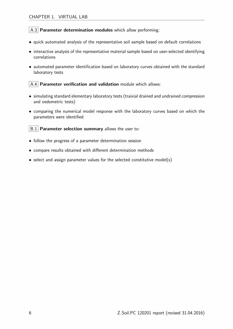
A.3 Parameter determination modules which allow performing:

• quick automated analysis of the representative soil sample based on default correlations

• interactive analysis of the representative material sample based on user-selected identifyingcorrelations

• automated parameter identification based on laboratory curves obtained with the standardlaboratory tests

A.4 Parameter verification and validation module which allows:

• simulating standard elementary laboratory tests (traixial drained and undrained compressionand oedometric tests)

• comparing the numerical model response with the laboratory curves based on which theparameters were identified

B.1 Parameter selection summary allows the user to:

• follow the progress of a parameter determination session

• compare results obtained with different determination methods

• select and assign parameter values for the selected constitutive model(s)


1.3. ELEMENTS

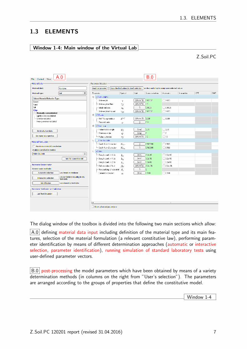
1.3 ELEMENTS

Window 1-4: Main window of the Virtual Lab

Z Soil.PC

A.0 B.0

The dialog window of the toolbox is divided into the following two main sections which allow:

A.0 defining material data input including definition of the material type and its main fea-tures, selection of the material formulation (a relevant constitutive law), performing param-eter identification by means of different determination approaches (automatic or interactiveselection, parameter identification), running simulation of standard laboratory tests usinguser-defined parameter vectors.

B.0 post-processing the model parameters which have been obtained by means of a varietydetermination methods (in columns on the right from ”User’s selection”). The parametersare arranged according to the groups of properties that define the constitutive model.

Window 1-4



Window 1-5: Material setup and parameter determination methods

Z Soil.PC

� Material label as in main Materialdialog of ZSoil

� General family of the material.Only Soils are available in v16

� Specification of Material Behavior Typeand a specific feature which drivesthe preselection assistant formaterial model formulation

�

Definition of field test dataSome in situ tests can helpto determine Material Behavior Type

� Definition of basic material properties specificto preselected Material Behavior Type

� Activation of the model formulation assistant.Model is recommended based on the preselectedMaterial Behavior Type.

� Calls automatic or interactive parameter selectionmodules - fully automatic or user-engagedparameter determination, respectively

�Calls parameter identification module- automated interpretation of laboratory curves.

� Allows running simulation of laboratory testsusing user-defined or automaticallyselected parameter vectors.

Window 1-5


1.3. ELEMENTS

Window 1-6: Post-processing - Parameter Summary

Z Soil.PC

B.1 B.2

B.3 B.4

B.5

Elements of the parameter selection summary:B.1 calls graphical post-processing results

B.2 copy parameter values which are assigned by means of different determination methods

( B.4 ) to the final selection ( B.3 )

B.3 values from the green column can exported to the main Material dialog ofZSoil when closing the parameter determination session (see Win.6-1)

B.5 fast assigning individual parameters with the aid of the drag-and-drop technique

Window 1-6



1.4 HOW TO PERFORM ...

1.4.1 ... PARAMETER DETERMINATION

1. Define Material Behavior Type

2. Define macroscopic general material behavior and available material properties and fieldtest data

3. Select the material formulation (constitutive model) that you would like to use

4. Perform parameter identification if complete laboratory experimental data are available

5. Perform Automatic Parameter Selection or/and Interactive Parameter Selection

6. Perform post-processing of identified results

7. Perform parameter verification or parameter validation by comparing numerical results withexperimental data

1.4.2 ... PARAMETER ESTIMATION

1. Define macroscopic general material behavior and available material properties and fieldtest data

2. Perform Automatic Parameter Selection or/and Interactive Parameter Selection

3. Perform parameter verification by running elementary laboratory tests

1.4.3 ... PARAMETER IDENTIFICATION

1. Select the material formulation that you would like to use and press the button Identification

2. Insert experimental data from laboratory tests

3. Go to data interpretation, select the test that you would like to interpret and press thebutton Interpret selected

4. Close the parameter identification dialog and perform post-processing of identified results

5. Perform parameter validation by comparing numerical results with experimental data

1.4.4 ... SIMULATION OF LABORATORY TEST

1. Select the material formulation (constitutive model) that you would like to use

2. Go to Laboratory Test Simulator

3. Choose the laboratory test that you would like to simulate

4. Define initial state variables

5. Define loading program


1.4. HOW TO PERFORM ...

6. Specify model parameters

7. Run simulation by pressing Run selected test


Chapter 2

MATERIAL DATA INPUT FOR SOILS

In the Virtual Lab, parameter determination algorithms identify material parameters basedon the user-delivered material data. These data can be specified by means of the two maindialog windows:

1. Basic material properties which allows specifying:

• General soil description

• Generic material properties

• Material type specific properties

2. In situ test data which allows specifying representative results derived from field tests aswell as, a quick, first-guess parameter estimation for the following commonly applied insitu tests:

• Cone Penetration Test (CPT)

• Marchetti’s Dilatometer Test (DMT)

• Menard’s Pressurementer Test (PMT)

• Standard Penetration Test (SPT)

• Shear wave velocity measurements (SWV)

CHAPTER 2. MATERIAL DATA INPUT FOR SOILS

2.1 BASIC MATERIAL PROPERTIES

The Basic Material Properties dialog boxes make possible to introduce all available data thatare known for the considered real material.

Window 2-1: Basic material properties for soil

Z Soil.PC

C.1

C.2 C.3

C.4

C.5

C.6

C.7

C.8

Window 2-1

C.1 General soil description which best defines observed macroscopic material behavior

C.2 Group of known parameters, common for any type of soil

C.3 Group of parameters specific to the soil type, e.g. granular or cohesive soils

C.4 If enabled, the general soil description will be automatically updated when known pa-rameters are specified or modified; if the general soil description is modified by changing anysoil feature and the value of parameter is not compatible with the soil feature criterion, thecell with the parameter value will be highlighted in redC.5 Input of material characteristics typically reported in geotechnical documentations

C.6 Auxiliary data used to compute e0, γD, γSAT , γB; they can be also used in manyempirical correlations when performing interactive parameter selectionC.7 Simplified soil stiffness description; during parameter selection, the specified modulus


2.1. BASIC MATERIAL PROPERTIES

will be kept unchanged, however its value will be transformed to the user defined refer-ence stress σref by applying the stiffness power law and corresponding minor stress which iscomputed based on the provided value of the vertical stress σ′v0 and evaluated in situ K0

coefficient.C.8 Importing tabular data collected in ASCII file.

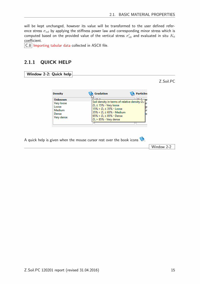
2.1.1 QUICK HELP

Window 2-2: Quick help

Z Soil.PC

A quick help is given when the mouse cursor rest over the book icons .

Window 2-2



2.1.2 GENERAL SOIL DESCRIPTION

The general soil description allows the identification algorithm to filter best-working correla-tions when performing Automatic Parameter Selection. The more precise soil description,the narrower the confidence limits for parameters.

Window 2-3: General soil description (1/2)

Z Soil.PC

Soil Behavior Type General soil type behavior according to the Unified Soil ClassificationSystem (USCS)

Stress History Overconsolidation state according to geotechnical convention:• 1.0 < OCR < 1.1 normally consolidated• 1.1 < OCR < 2.5 lightly overconsolidated• 2.5 < OCR < 5.0 overconsolidated• OCR > 5.0 heavily overconsolidated

Density/Consistency Relative soil density or soil consistency depending on general soil typebehavior

Coarse-grained soil classification in terms of relative density Dr:• Dr <= 15% - Very loose• 15% < Dr <= 35% - Loose• 35% < Dr <= 65% - Medium• 65% < Dr <= 85% - Dense• Dr > 85% - Very dense

Fine-grained soil classification in terms of consistency index IC (=(wL − w)/PI):• IC < 0.05 - Very soft• 0.05 < IC < 0.25 - Soft• 0.25 < IC < 0.75 - Medium• 0.75 < IC < 1.00 - Stiff• IC > 1.00 and w > ws - Very Stiff• IC > 1.00 and w < ws - Hardwith w - moisture content, ws - shrinkage limit

Window 2-3



Window 2-4: General soil description (2/2)

Z Soil.PC

Gradation/Plasticity Gradation of coarse-grained soil or plasticity of fine-grained soil

Coarse-grained soil classification in terms of gradation:• Poorly-graded sands Cu ≤ 6 (and/or Ck < 1 Ck > 3)• Poorly-graded gravels Cu ≤ 4 (and/or Ck < 1 Ck > 3)• Well-graded sands Cu ≤ 6 (and 1 ≤ Ck ≤ 3)• Well-graded gravels Cu ≤ 4 (and 1 ≤ Ck ≤ 3)with Ck - coefficient of curvature, Cu - coefficient of uniformityIf the content of fines (particles smaller than 0.06mm) is larger than12% then coarse-grained soil may be classified as silty or clayey:• Silty if PI < 4 or Atterberg limits below ”A” line in the plasticitychart ( ”A” line: PI = 0.73(wL − 20) )• Clayey if PI > 7 or Atterberg limits above ”A” line in the plasticitychart.

Fine-grained soil classification in terms of plasticity and liquid limitwL:• 0 < wL ≤ 35% - Low plasticity• 35 < wL ≤ 50% - Medium plasticity• 50 < wL ≤ 70% - High plasticity• 70 < wL ≤ 90% - Very high plasticity• wL > 90% - Extremely high plasticity

Shape/Organics Shape of particles of a coarse-grained soil or existence of organicscontent in a fine-grained soil

General classification in terms of organics content:• Inorganic soil OC ≤ 3%• Organic silt or clay 3 < OC ≤ 10%• Medium organic soils 10 < OC < 30% (not supported in v2016)• Highly organic soils OC > 30% (not supported in v2016)

This classification affects the prediction of deformation characteristicsState State of soil saturation

Automatic Parameter Selection estimates always two types of unitweight:1. Dry unit weight γD (used in Deformation+Flow analysis type)2. Apparent unit weight γ based on the specified degree of saturationS (the apparent weight is used in Deformation analysis type)

NB. For the Deformation+Flow analysis type, the apparent unitweight of each finite element is computed from the current degree ofsaturation S and porosity n:γ = γD + nSγF with γF - fluid unit weight

Window 2-4



2.1.3 AUXILIARY NUMERIC DATA

The dialog allows specifying known values for material characteristics typically reported inthe geotechnical reports. Some of these parameters are used to adjust the general soil de-scription and can appear as the input in correlations which help to compute or estimate otherparameters. Note that the user-defined parameters which describe the representative mate-rial sample will remain fixed and unchanged during any automatic or interactive parameterselection session.

Window 2-5: Content of Known soil properties group and its description

Z Soil.PC

Friction angle φ Effective friction angle; if specified, it is used to estimate KNC0 and

K0.Cohesion c Effective cohesion which may account for effect of soil cementation

(typically for remoulded and saturated soil c ≈ 0 and the effect ofpartial saturation, i.e. an apparent cohesion due to suction, canbe controlled by parameters α and Sr which define the behavior ofpartially saturated medium).

Overconsolidationratio

OCR Value of OCR which corresponds to the provided representative pa-rameters E, φ, c derived at corresponding characterization depth.Specifying or modifying OCR updates Stress History setup which istaken into account in estimation of Eref

0 for coarse-grained soils.Unit weight γ Total unit weight corresponding to the natural moisture content wn.

Its magnitude with the value of natural moisture content wn’ andsaturation degree S, is used to compute dry unit weight γD.In the numerical analysis, γ is used to describe the total soil unitweight for the single phase analysis (Deformation only).If specified, the value will be fixed during automatic or interactiveparameter selection.

Initial void ratio e0 Estimated void ratio at in situ stress condition. The number will beautomatically updated once n0 has been modified in the Physical SoilProperties table.Any change of e0 will update γSAT if γD and γ are introduced bethe user.

Window 2-5



Weight of dry soil/weight of saturatedsoil

γD /γSAT

γD corresponds to ”dry” soil state when the degree of saturationis equal to 0 (in the Deformation+flow analysis type, γD is usedto calculate total unit weight accounting for saturation degree),whereas γSAT is the weight of fully saturated soil (S = 1).The unit weight of a dry soil γD can computed based on thespecified values of apparent unit weight γ and saturation degreeS and voids ratio e0 from: γ = γD+nSγw where n = e0/(1+e0).Moreover γSAT will be updated if e0 or n0 have been specified ormodified.γD and γSAT are also the inputs for some correlations whichestimates the compression index Cc.

Buoyant unit weight γB The buoyant unit weight (or effective unit weight) of soil is ac-tually the saturated unit weight of soil minus the unit weight ofwater. Its value can be used to describe the effective soil weightof the soil below the ground water table when running the single-phase analysis considered as the effective stress analysis.

Reported stiffnessmodulus

E The stiffness modulus which is typically delivered in simplifiedgeotechnical reports which provide a single modulus to describesoil stiffness. The modulus must correspond to the vertical ef-fective stress σ′

v0 at characterization depth or in the middle of arelatively thin geotechnical layer. Since the soil stiffness can bedescribed by many different moduli, the user can precise to whichtype of modulus, the reported modulus corresponds to.The reported E is taken to estimate Eref

s , Eref50 , Eref

ur and Eref0 .

• ”Static” modulus Es In this case, it is assumed that the specified modulus is consideredto be the stiffness modulus measured at the initial part of the ε1−qtriaxial curve (at ε1 ≈ 0.1%). Note that E50 < Es < Eur.

• Unloading -reloading modulus

Eur In this case, the specified modulus is considered as the modulustaken from the unloading/reloading part of the triaxial curve ε1−qor other test which allowed the stiffness modulus to be measuredin unloading/reloading test conditions.

• Secant modulus E50 In this case, the specified modulus is considered as that represent-ing the secant stiffness measured at 50% of the failure deviatoricstress qf = σ1 − σ3. If no indication about the genesis of E hasbeen provided, such an approach is the least conservative.

Vert. eff. stressat characterizationdepth or in themiddle of soil layer

σ′v0 Estimated vertical effective stress at characterization depth; if not

indicated σ′v0 can be taken as the effective stress in the middle of a

representative soil layer. The stiffness moduli which are estimatedbased on the provided ”reported” stiffness modulus will be scaledto the user-defined reference stress σref with respect to the minoreffective stress estimated as σ3 = min(σ′

v0, σ′v0 · K0). If σ′

v0 isnot specified, the minor stress will be taken equal to the user-defined reference σ3 = σref kPa (no stiffness scaling applies).



Window 2-6: Content of Physical soil properties and its description

Z Soil.PC

Physical soil properties can be used for calculating:e0 = γs/γW ·wn/S for S > 0γD = γ − n0SγWe0 = n0/(1 − n0)

Unit weight of materialskeleton

γs Typical values of Gs = solid density / water density:

• Gravel - quartz 2.65• Gravel - silty or clayey 2.66 − 2.68• Sand - quartz 2.65• Sand - silty or clayey 2.66 − 2.68• Silt, inorganic 2.62 − 2.68• Clay of low plasticity, inorganic 2.67 − 2.70• Clay of medium plasticity, inorganic 2.69 − 2.72• Clay of high plasticity, inorganic 2.71 − 2.78• Clay, organic 2.58 − 2.65

γs also appears in some correlations for Cc.Natural moisture content wn Typical void ratio and water content when saturated:

Soil description: wsat (%) and e (-)• Poorly graded sand: 32 and 0.85• Poorly-graded sand dense: 19 and 0.51• Well-graded sand, loose: 25 and 0.67• Well-graded sand, dense: 16 and 0.43• Glacial till, very mixed-grained: 9 and 0.25• Soft glacial clay: 45 and 1.2• Stiff glacial clay: 22 and 0.6• Soft slightly organic clay: 70 and 1.9• Soft very organic clay: 110 and 3.0• Soft bentonite: 194 and 5.2

The value wn is used to calculate porosity n0 and e0:e0 = γS/γW · wn/S for S > 0wn also appears in some correlations which estimatesthe compression index Cc.

Degree of saturation S Measured or estimated degree of soil saturation at insitu stress conditions.Introducing or changing the value of S updates Statesetup.The value S is used to calculate dry unit weight fromγD = γS · n0 · γW .

Initial porosity n0 Estimated porosity at in situ stress conditions.

Window 2-6



Window 2-7: Content of Soil type specific properties for fine-grained soils

Z Soil.PC

Fine-grained soilsFines content fp Content of particles smaller than 0.06 mm.

If fp > 50% then soil is classified as fine-grained (cohesive)otherwise as coarse-grained.

Organics content fp General classification in terms of organics content:- inorganic soil OC ≤ 3%- organic silt or clay 3 < OC ≤ 10%- medium organic soils 10 < OC < 30% (not supported inv2016)- highly organic soils OC ≥ 30% (not supported in v2016)

Plasticity index PI PI = wL − wP is taken to estimate γ0.7 and appears insome correlations for φ, m, KNC

0 and Cc.Liquid limit wL Introducing or modifying the value of wL updates Soil

plasticity:• Low plasticity wL ≤ 35%• Medium plasticity 35 < wL ≤ 50%• High plasticity 50 < wL ≤ 70%• Very high plasticity 70 < wL ≤ 90%• Extremely high plasticity wL > 90%The specified value appears in some correlations for stiff-ness exponent m and compression index Cc.

Plastic limit wP Plastic limit is computed from:wP = wL − PIonce both variables have been specified.The value of wP can be used in some correlations to cor-relate the small strain threshold γ0.7 or compression indexCc.

Consistency index Ic Consistency index helps to automatically update Soil con-sistency.Its value is computed from Ic = (wL − wn)/PI once wn,wL and PI have been specified-

Window 2-7



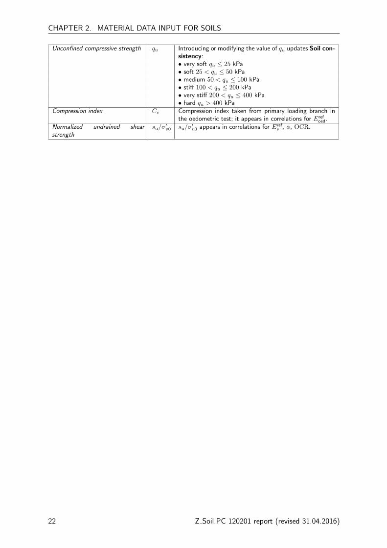
Unconfined compressive strength qu Introducing or modifying the value of qu updates Soil con-sistency:• very soft qu ≤ 25 kPa• soft 25 < qu ≤ 50 kPa• medium 50 < qu ≤ 100 kPa• stiff 100 < qu ≤ 200 kPa• very stiff 200 < qu ≤ 400 kPa• hard qu > 400 kPa

Compression index Cc Compression index taken from primary loading branch inthe oedometric test; it appears in correlations for Eref

oed.Normalized undrained shearstrength

su/σ′v0 su/σ

′v0 appears in correlations for Eref

s , φ, OCR.



Window 2-8: Content of Soil type specific properties for coarse-grained soils

Z Soil.PC

Coarse-grained soilsFines content fp Content of particles smaller than 0.06 mm.

If 12% < fp < 50% then coarse-grained soil may be clas-sified as silty or clayey:- Silty if PI < 4% or Atterberg limits below ”A” line inthe plasticity chart- Clayey if PI > 7% or Atterberg limits above ”A” line inthe plasticity chart”A” line: PI = 0.73(wL − 20)If fp > 50% then soil is classified as fine-grained (cohe-sive).

Coefficient of uniformity Cu Cu = d60/d10 is used to define soil gradation.

Typical values of Cu for uniform (poorly-graded) materials:• Equal spheres 1.0• Standard Ottawa sand 1.1• Clean, uniform sand (fine or medium) 1.2 to 2.0• Uniform, inorganic silt 1.2 to 2.0• Poorly-graded sands ≤ 6 (and/or Ck < 1, Ck > 3)• Poorly-graded gravels ≤ 4 (and/or Ck < 1, Ck > 3)

Typical values of Cu for well-graded materials:• Silty sand 5 to 10• Silty sand and gravel 15 to 300• Well-graded sands > 6 (and 1 ≤ Ck ≤ 3)• Well-graded gravels > 4 (and 1 ≤ Ck ≤ 3)

Cu appears in a correlation estimating ranges of e forcoarse-grained materials.

Coefficient of curvature Ck Ck = d230/(d10d60) is used to define soil gradation.d10 - the maximum size of the smallest 10% of the sampled30 - the maximum size of the smallest 30% of the sampled60 - the maximum size of the smallest 60% of the sample

• Ck between 1.0 and 3.0 indicates a well-graded soil• Ck < 1 or Ck > 3.0 indicates poorly-graded soil

Relative density Dr Introducing or changing the value of Dr updates soil den-sity setup.The specified value is used to estimate φ, ψ and e0.

Window 2-8



Window 2-9: Importing data from ASCII file

Z Soil.PC

The values of soil characteristics can be prepared in advance for a number of geotechnical layers (rows) andimported from any ASCII file (*.csv, *.txt). The header in the import wizard table allows attributing the soilcharacteristics to the corresponding parameters collected in columns. Only the values in the selected row(checked row) will be imported.

Window 2-9


2.2. IN SITU TEST DATA

2.2 IN SITU TEST DATA

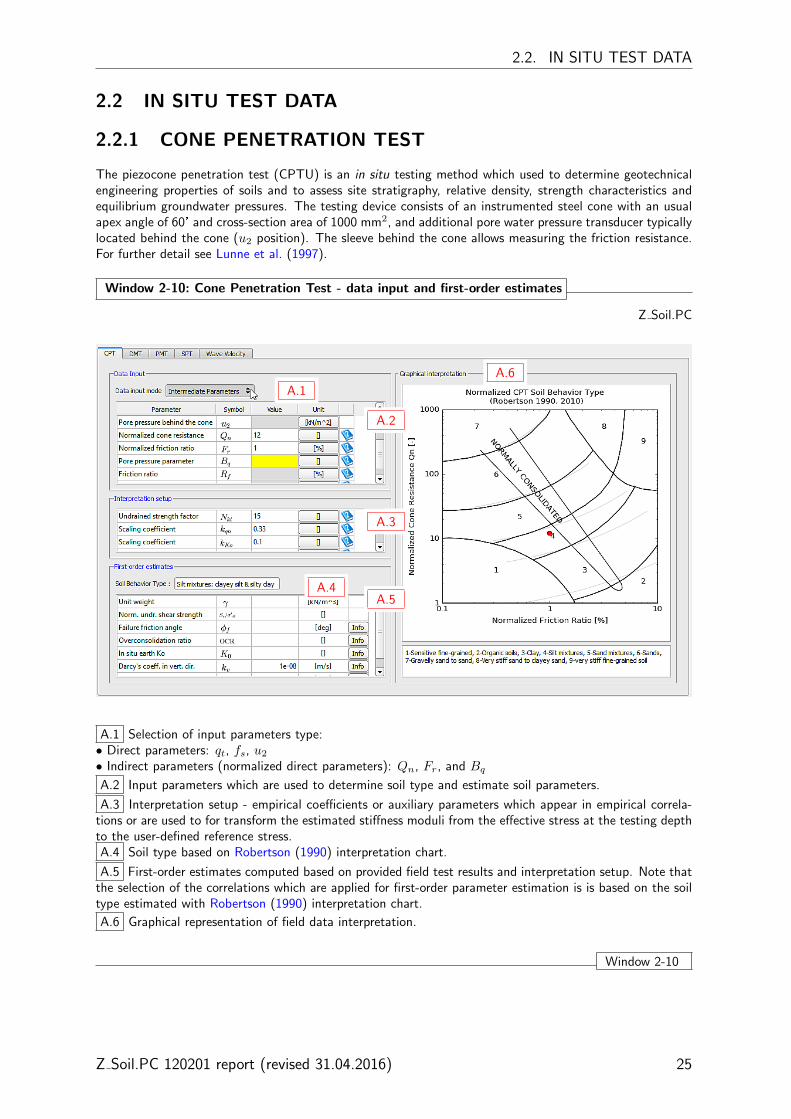
2.2.1 CONE PENETRATION TEST

The piezocone penetration test (CPTU) is an in situ testing method which used to determine geotechnicalengineering properties of soils and to assess site stratigraphy, relative density, strength characteristics andequilibrium groundwater pressures. The testing device consists of an instrumented steel cone with an usualapex angle of 60° and cross-section area of 1000 mm2, and additional pore water pressure transducer typicallylocated behind the cone (u2 position). The sleeve behind the cone allows measuring the friction resistance.For further detail see Lunne et al. (1997).

Window 2-10: Cone Penetration Test - data input and first-order estimates

Z Soil.PC

A.1

A.2

A.3

A.4A.5

A.6

A.1 Selection of input parameters type:• Direct parameters: qt, fs, u2• Indirect parameters (normalized direct parameters): Qn, Fr, and Bq

A.2 Input parameters which are used to determine soil type and estimate soil parameters.

A.3 Interpretation setup - empirical coefficients or auxiliary parameters which appear in empirical correla-tions or are used to for transform the estimated stiffness moduli from the effective stress at the testing depthto the user-defined reference stress.A.4 Soil type based on Robertson (1990) interpretation chart.

A.5 First-order estimates computed based on provided field test results and interpretation setup. Note thatthe selection of the correlations which are applied for first-order parameter estimation is is based on the soiltype estimated with Robertson (1990) interpretation chart.

A.6 Graphical representation of field data interpretation.

Window 2-10



Cone Penetration Test (CPT/CPTU)Corrected cone resistance qt The corrected cone tip resistance qt is calculated as:

qt = qc + (1 − an)u2 where:qc - measured cone resistancean - net area ratio of the cone (see Lunne et al., 1997)

qt together with σv0 and u0 is used to automatically com-pute Qt if the latter is not directly specified.qt is also used to determine the soil behavior type and unitweight.qt appears in correlations for E0, Vs, E50, φ in coarse-grained soil, and Vs, Eoed, φ, OCR, K0 in fine-grainedsoils.

Pore pressure behind thecone

u2 This number is used to calculate Bq.

u2 appears in correlations for OCR in fine-grained soils.Friction sleeve resistance fs Unit sleeve friction resistance.

fs together with qt and σv0 is used to automatically com-pute Fr if the latter is not directly specified.fs is also used to determine the soil behavior type and unitweight.fs appears in correlations for Vs

Total vertical stress σv0 Estimated total vertical stress corresponding to the in situstress level at which the CPT measurements have beentaken.

σv0 appears in correlations estimating Eoed, OCR in fine-grained soils and is used to compute the effective verticalstress σ′

v0 = σv0 − u0Hydrostatic pore pressure u0 Hydrostatic pore pressure at testing level. This number

is used to calculate Bq and effective vertical stress fromσ′v0 = σv0 − u0

Effective vertical stress σ′v0 Calculated as σ′

v0 = σv0 − u0.σ′v0 is needed to transform the estimated stiffness moduli to

the reference modulus Eref by accounting for the referencestress σref and K0 (cf. Win.2-15).

Dimensionless unit weight γCPT

/γW

Proposed using the relationship proposed by Robertson andCabal (2010) based on qt and fs: γ/γW = 0.27 logRf +0.36 log (qt/pa) + 1.236, with pa = 100 kPa being atmo-spheric pressure and Rf = fs/qt ·100% is the friction ratio.This number can be used to estimate apparent unit weight:γ = γCPT (γW = unit weight of water).

Normalized cone resistance Qt Qt = (qt − σv0)/σ′v0

Qt appears in correlations estimating φ, K0 for for fine-grained soils.

Normalized pore pressureparameter

Bq Bq = (u2 − u0)/(qt − σv0)

Bq appears in correlations estimating φ for for fine-grainedsoils.

Normalized friction ratio Fr Fr = fs/(qt − σv0)Soil type behavior Determined based on Qt and Fr numbers using the original

chart by Robertson (1990)



2.2.2 MARCHETTI’S DILATOMETER TEST

The flat dilatometer, or DMT, is an in-situ device used to determine the soil in-situ lateral stress and soillateral stiffness and to estimate some other engineering properties of subsurface soils (Marchetti et al., 2001).A dilatometer test consists of pushing a flat blade located at the end of a series of rods. Once at the testingdepth, a circular steel membrane located on one side of the blade is expanded horizontally into the soil. Thepressure is recorded at specific moments during the test. The blade is then advanced to the next test depth.

Window 2-11: Marchetti’s Dilatometer Test - data input and first-order estimates

Z Soil.PC

B.1

B.2

B.3

B.4B.5

B.6

B.1 Selection of input parameters type:• Direct parameters: p0, p1• Indirect parameters (normalized direct parameters): ED, IDB.2 Input parameters which are used to determine soil type and estimate soil parameters.

B.3 Interpretation setup - empirical coefficients or auxiliary parameters which appear in empirical correla-tions or are used to for transform the estimated stiffness moduli from the effective stress at the testing depthto the user-defined reference stress by appling stress stiffness dependency law.

B.4 Soil type based on material index ID (Marchetti, 1980).

B.5 First-order estimates computed based on provided field test results and interpretation setup. Note thatthe selection of the correlations which are applied for first-order parameter estimation is is based on the soiltype estimated with the material index ID (Marchetti, 1980).

B.6 Graphical representation of field data interpretation.

Window 2-11



Marchetti’s Dilatometer Test (DMT)First DMT reading p0 Corrected pressure which is required to start moving the

membrane towards soil. The correction accounts for mem-brane stiffness.The value is used to calculate the dilatometer numbers ID,KD and ED.

Second DMT reading p1 Corrected pressure which is required to move the center ofthe membrane 1.1 mm into soil.The value is used to calculate the dilatometer numbers IDand ED.

Hydrostatic pore pressure u0 Hydrostatic pore pressure at the testing depth.The value is used to calculate the dilatometer numbers IDand KD.

Effective in situ verticalstress

σ′v0 Estimated effective vertical stress corresponding to the in

situ stress level at which the DMT measurements havebeen taken.This number is needed to transform an estimated valueof stiffness modulus to the reference modulus Eref takinginto account the reference stress σref, K0 and the powerlaw (cf. Win.2-15).

Material index ID ID = (p1 − p0)/(p0 − u0)used for determination of soil type behavior (Marchetti,1980):• ID < 0.6 - Clay• 0.6 ≤ ID < 1.8 - Silt• 1.8 ≤ ID < 3.3 - Silty sand• 3.3 ≤ ID < 8 - Sand

ID is used to provide estimations of soil behavior type andunit weight.ID appears in correlations estimating Eoed in normally-consolidated soils.

Horizontal stress index KD KD = (p0 − u0)/σ′v0

KD appears in correlations estimating Eoed in normally-consolidated soils, φ for coarse-grained soil, and OCR, K0

for fine-grained soil.Dilatometer modulus ED ED = 34.7(p1 − p0)

ED is used to provide estimations of unit weight.ED appears in correlations estimating Eref

oed in normally-consolidated soils, φ for coarse-grained soil.

Dimensionless unit weight γDMT

/γW

Estimated based on provided ID and ED numbers usingthe original chart for estimating soil type and unit weightby Marchetti and Crapps (1981). This number can be usedto estimate apparent unit weight: γ = γDMT (γW = unitweight of water).



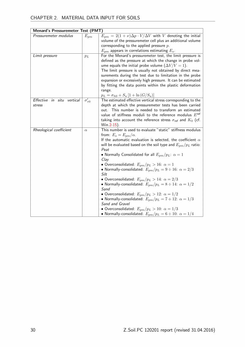
2.2.3 MENARD’S PRESSUREMETER TEST

The pressuremeter test is an in situ testing method used to achieve a quick measure of the in situ stress-strainrelationship of the soil (Mair and Wood, 1987). The principle is to introduce a cylindrical probe with a flexiblcover which can expand radially in a borehole. A pressure is applied by the probe on the sidewalls of thehole, and soil deformation is measured, through the acquisition of the hole volume increase.

Window 2-12: Menard’s pressuremeter test - data input and first-order estimates

Z Soil.PC

C.1

C.2

C.3

C.1 Input parameters which are used to determine stiffness modulus.

C.2 Interpretation setup - auxiliary parameters which are used to for transform the estimated stiffness mod-ulus from the vertical effective stress at the testing depth to the user-defined reference stress by applying thestress stiffness dependency law.

C.3 First-order estimates computed based on provided input data and interpretation setup.

Window 2-12



Menard’s Pressuremeter Test (PMT)Pressuremeter modulus Epm Epm = 2(1 + ν)∆p · V/∆V with V denoting the initial

volume of the pressuremeter cell plus an additional volumecorresponding to the applied pressure p.Epm appears in correlations estimating Es.

Limit pressure pL For the Menard’s pressuremeter test, the limit pressure isdefined as the pressure at which the change in probe vol-ume equals the initial probe volume (∆V/V = 1).The limit pressure is usually not obtained by direct mea-surements during the test due to limitation in the probeexpansion or excessively high pressure. It can be estimatedby fitting the data points within the plastic deformationrange.pL = σh0 + Su [1 + ln (G/Su)]

Effective in situ verticalstress

σ′v0 The estimated effective vertical stress corresponding to the

depth at which the pressuremeter tests has been carriedout. This number is needed to transform an estimatedvalue of stiffness moduli to the reference modulus Eref

taking into account the reference stress σref and K0 (cf.Win.2-15).

Rheological coefficient α This number is used to evaluate ”static” stiffness modulusfrom: Es = Epm/α.If the automatic evaluation is selected, the coefficient αwill be evaluated based on the soil type and Epm/pL ratio:Peat• Normally Consolidated for all Epm/pL: α = 1Clay• Overconsolidated: Epm/pL > 16: α = 1• Normally-consolidated: Epm/pL = 9 ÷ 16: α = 2/3Silt• Overconsolidated: Epm/pL > 14: α = 2/3• Normally-consolidated: Epm/pL = 8 ÷ 14: α = 1/2Sand• Overconsolidated: Epm/pL > 12: α = 1/2• Normally-consolidated: Epm/pL = 7 ÷ 12: α = 1/3Sand and Gravel• Overconsolidated: Epm/pL > 10: α = 1/3• Normally-consolidated: Epm/pL = 6 ÷ 10: α = 1/4



2.2.4 STANDARD PENETRATION TEST

The standard penetration test (SPT) is an in-situ dynamic penetration test designed toprovide information on the geotechnical engineering properties of soil. The test uses a thick-walled sample tube, with an outside diameter of 50.8 mm and an inside diameter of 35 mm,and a length of around 650 mm. This is driven into the ground at the bottom of a boreholeby blows from a slide hammer with a mass of 63.5 kg (140 lb) falling through a distance of760 mm (30 in). The sample tube is driven 150 mm into the ground and then the numberof blows needed for the tube to penetrate each 150 mm (6 in) up to a depth of 450 mm(18 in) is recorded. The sum of the number of blows required for the second and third 6 in.of penetration is termed the ”standard penetration resistance” or the ”N-value”. The blowcount provides an indication of the density of the soil, approximation of shear strength andstiffness properties, and it is used in many empirical geotechnical engineering formulas.

Window 2-13: Standard Penetration Test - data input and first-order estimates

Z Soil.PC

D.1

D.2

D.3

D.1 Input parameters which are used to determine soil density or consistency, and to esti-mate soil parameters.D.2 Interpretation setup - empirical coefficients or auxiliary parameters which appear in

empirical correlations or are used to for transform the estimated stiffness moduli from theeffective stress at the testing depth to the user-defined reference stress.D.3 First-order estimates computed based on provided field test results and interpretation

setup.



Window 2-13

Standard Penetration Test (SPT)Number of blows N60 Number of blows to drive the sampler the last two 150mm distances (300mm in

total) to obtain the N number.N60 corresponds to the energy ratio Er = 60. Since the energy × blow countshould be a constant for any soil, the following equation can be applied Er1×N1 =Er2 ×N2 (Bowles, 1997). For example, N55 = N60 × 60/55.Introducing or modifying N60 prompts the user to update Soil density group forcoarse-grained soil or Soil consistency for fine-grained soil.• Relative soil density based on N60:0− 4 Very loose; 5− 10 Loose ; 11− 30 Medium; 31− 50 Dense; > 50 Very dense• Soil consistency based on N60:0 − 2 Very soft; 3 − 4 Soft; 4 − 8 Medium; 9 − 15 Stiff; 16 − 30 Very Stiff; > 30HardN number appears in correlations for coarse-grained soils to estimate Eur, φ, Vs.

Effective verticalstress

σ′v0 The estimated effective vertical stress corresponding to the in situ stress level at

which the number N60 has been measured. This number is needed to calculatestress overburden coefficient CN and to transform the estimated stiffness modulito the reference modulus Eref by accounting for the reference stress σref and K0

(cf. Win.2-15).Overburden cor-rection factor

CN Overburden correction factor is calculated according to Liao and Whitman (1986)

as CN = (pa/σ′v0)

0.5(CN = 1.7 if CN > 1.7) with pa - atmospheric pressure =

100 kPa once σ′v0 is provided for SPT.

Corrected N60 N60,1 Corrected SPT N value for overburden stress with respect to 100 kPaN60,1 = N60 × CN



2.2.5 SHEAR WAVE VELOCITY

Characterization of the small-strain shear modulus and the shear wave velocity of soils and rocks is an integralcomponent of various static and dynamic analyzes of soil-structure interaction. The shear wave velocity canbe measured by a variety of testing methods:

• seismic piezocone testing (SCPTU) (Campanella et al., 1986)

• seismic flat dilatometer test (SDMT) (Marchetti et al., 2008)

• cross hole, down hole seismic tests

• geophysical tests (Long, 1998):

F continuous surface waves (CSW)

F spectral analysis of surface waves (SASW)

F multi-channel analysis of surface waves (MASW)

F frequency wave number (f-k) spectrum method

Window 2-14: Shear Wave Velocity - data input and first-order estimates

Z Soil.PC

C.1

C.2

C.3

E.1 Input parameters which are used to determine maximal shear modulus.

E.2 Interpretation setup - auxiliary parameters which are used to for transform the estimated stiffness mod-ulus from the vertical effective stress at the testing depth to the user-defined reference stress.

E.3 First-order estimates computed based on provided input data and interpretation setup.



Window 2-14

Shear wave velocityShear wave velocity Vs If specified, the value is taken into account in Automatic

Parameter Selection for estimation of E0 = 2G0(1 + νur)by applying G0 = ρV 2

s .Unit weight γ Total unit weight.Effective in situ verticalstress

σ′v0 Estimated effective vertical stress corresponding to the in

situ stress level at which measurements of Vs have beentaken. σ′

v0 and auxiliary parameters are used to transformthe computed E0 value to the user-defined reference stressσref according to the principle illustrated below Win.2-15).



2.2.6 STIFFNESS MODULI TRANSFORMATION

Window 2-15: Principle of transformation for stiffness moduli

Z Soil.PC

Stiffness moduli derived from in situ test data for a given charaterization depth are adjusted with respect tothe depth that corresponds to σref using stiffness stress dependency law, as illustrated below:

The transformation of stiffness moduli to the reference ones, i.e. those corresponding to the user-definedreference stress, is carried out by applying the following power law:

Eref =E(

σ3 + a

σref + a

)m (1)

where:- Eref is the target modulus corresponding to the user-defined reference stress σref

- E: the modulus identified for a given minor stress state σ3

- m: stiffness exponent (typically between 0.5 and 1.0)- σ3 = min(σ′

v0, σ′v0 ·K0)

- a = c · cot(φ)

Window 2-15


Chapter 3

MATERIAL FORMULATIONSELECTION

The assistance in model preselection allows less experienced users to chose a suitable materialformulation to describe the material behavior. By activating the automatic preselection, thecombobox will contain constitutive models which are considered to be adequate for theselected material behavior type and basic feature. In the case of soils, the preconsolidation isthe main criterion of model selection. For example, modeling of normally-consolidated andlightly overconsolidatated deposits requires applying a model which accounts for volumetricplastic straining. In this case, only the models with the cap mechanism will be suggested.The suggested material formulation are arranged in the combobox list in order of adequacy.

Window 3-1: Material formulation

Z Soil.PC

A.1

A.2

A.1 Input parameters which are used to determine maximal shear modulus.

A.1 The combobox contains a list of available (or suggested, if assistance in preselectionenabled) constitutive models.

Window 3-1

CHAPTER 3. MATERIAL FORMULATION SELECTION


Chapter 4

PARAMETER DETERMINATION

Parameter determination refers to an effective assessment of design soil properties whichallow us to reproduce soil behavior by means of a numerical analysis assuming that an ade-quate constitutive model has been chosen.

The Virtual Lab offers the possibility of parameter determination including first-guess formodel parameters for any incomplete or complete material data, as well as an automatedparameter identification from laboratory curves.

Three general approaches can be applied to determine material model parameters:

• Automatic parameter selection

• Interactive parameter selection

• Parameter identification

The automatic parameter selection consists of applying a fully-automated algorithm toestimate model parameters based on provided general soil description. In this case, param-eter estimation refers here to the evaluation of model parameters from observed limits forparameter values which are extracted from an expert database. The module allows the userto have an insight into the correlations which have been used during automatic knowledgeextraction.

The interactive parameter selection offers the possibility of a manual knowledge extrac-tion. The user can consciously browse the correlations database looking for best-working cor-relations for the analyzed ”material sample”. These correlations relate geotechnical propertiesor measurements with constitutive model parameters. The correlations database contains thefollowing general groups of empirical correlations:

• those based on confidence limits for model parameters being the function of macroscopicsoil features (general soil description),

• those obtained through statistical regression analyzes, which relates known numeric data(geotechnical properties or field test results) with constitutive model parameters,

• mixed approaches based on macroscopic soil description and numeric data.

CHAPTER 4. PARAMETER DETERMINATION

Parameter identification refers to deterministic algorithms which are developed for givenconstitutive model and test geometry. These analytical solutions offer the direct identificationof model parameters from test measurements.


4.1. AUTOMATIC PARAMETER SELECTION

4.1 AUTOMATIC PARAMETER SELECTION

The Automatic Parameter Selection offers the possibility of a fully-automated estimation ofmodel parameters based on provided general soil description and numeric data.

Note that the automatic parameter selection relies on statistical data and empiricalcorrelations. It is user’s responsibility to verify the suitability of parameters for agiven purpose, in particular by verifying reproducibility of available experimentalresults and by adjustment of parameters.

Window 4-1: Performing automatic parameter selection

Z Soil.PC

A.0

B.0

C.0

A.1

A.2

A.3

A.4

In order to run automatic parameter selection:1. Specify general soil description and given numeric data2. Open the automatic parameter selection dialog A.0

3. Verify the general soil description A.1 and known numeric data A.2 . Note that theuser-predefined parameters will be highlighted in blue. They will be fixed and unchangedduring the automatic parameter selection. The fixed parameter values will also be used bycorrelations for the inter-correlated parameters (parameters that are identified based on thefixed parameters).

4. Run the automatic selection with A.3 . The window A.4 will inform about the progressof automatic selection, as well as, about the number of applicable correlations.

Window 4-1



Window 4-2: Viewing the results of automatic parameter selection

Z Soil.PC

A.5

A.6

A.7

• The results of performed automatic selection are summarized in A.5• The correlations which have been applied during automatic selection can be viewed byclicking on A.6

• A.7 simplifies attributing parameter estimations to model parameters (final user’s selec-tion in the main dialog of the Virtual Lab) after closing the dialog window. If disabled,the parameter estimations will appear in the column ’Automatic’; such a strategy makes itpossible to consciously choose the values for individual model parameters in the final ”user’sselection”.

Window 4-2


4.1. AUTOMATIC PARAMETER SELECTION

Window 4-3: Correlations applied during parameter selection

Z Soil.PC

A.8 A.9A.10

A.11

A.12

A.13

A.14

A.15

A.16

A.17

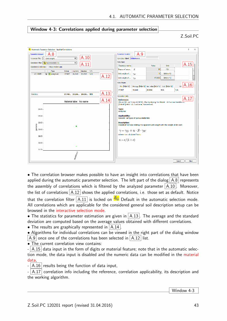
• The correlation browser makes possible to have an insight into correlations that have beenapplied during the automatic parameter selection. The left part of the dialog A.8 represents

the assembly of correlations which is filtered by the analyzed parameter A.10 . Moreover,

the list of correlations A.12 shows the applied correlations, i.e. those set as default. Notice

that the correlation filter A.11 is locked on Default in the automatic selection mode.All correlations which are applicable for the considered general soil description setup can bebrowsed in the interactive selection mode.• The statistics for parameter estimation are given in A.13 . The average and the standarddeviation are computed based on the average values obtained with different correlations.• The results are graphically represented in A.14 .• Algorithms for individual correlations can be viewed in the right part of the dialog windowA.9 once one of the correlations has been selected in A.12 list.• The current correlation view contains:- A.15 data input in the form of digits or material feature; note that in the automatic selec-tion mode, the data input is disabled and the numeric data can be modified in the materialdata,- A.16 results being the function of data input,

- A.17 correlation info including the reference, correlation applicability, its description andthe working algorithm.

Window 4-3



4.2 INTERACTIVE PARAMETER SELECTION

The Interactive Parameter Selection offers the possibility of a manual knowledge extraction.The user can consciously browse the correlations database looking for best-working correla-tions for the analyzed ”soil sample” and testing correlations by modifying input data.

Window 4-4: Performing interactive parameter selection

Z Soil.PC

A.0

B.0C.0

B.1 B.2

In order to perform an interactive parameter selection:1. Specify general soil description and known numeric data2. Open the interactive parameter selection dialog B.03. Before opening the correlation browser, the user will be prompted to choose between:• B.1 guided parameter selection with the aid of the identification wizard; in this modethe algorithm follows the parameter identification sequence which accounts for dependenciesbetween parameters (some parameters require prior identification of other parameters).

• B.2 unconstrained exploring of correlation browser; in this mode the parameter filter is

enabled B.4 .Note that in the interactive selection mode, the correlations can be filtered according to thefollowing criteria B.5 : All applicable, Default (those set as default ones) and Favorite (thosepreferred by the user and saved in the global configuration file).

B.3B.4B.5

Window 4-4


4.2. INTERACTIVE PARAMETER SELECTION

Window 4-5: Interactive parameter selection without estimation wizard

Z Soil.PC

B.6

B.7

B.8

B.9

B.10

B.11

B.12

B.13

B.14

B.15

4. During, the unconstrained interactive parameter selection the parameter filter B.6 re-mains unlocked.5. Model parameters which are predefined in material data input can be controlled by pressingthe button B.8

6. Suitable correlations can be selected in the correlations assembly B.9 by setting check-boxes active.7. Resulting average value and confidence limits B.10 can be quickly copied to the ”User’sselection” using Copy from Statistics button.8. The results are graphically represented in B.11 .9. The parameters values which from ”User’s selection” will appear in the column ’Interac-tive’ (in the main window of the Virtual Lab ) after closing the correlation browser.

The current correlation view contains:- data input in the form of digits B.13 or material feature B.12 ; parameters which are not

pre-defined in advance can be introduced in input cells B.9 , whereas the pre-defined onesremain locked and the input cells are gray.- results being function of data input B.16 ,

- correlation info B.15 including the reference, correlation applicability, its description andthe working algorithm.

Window 4-5



4.3 PARAMETER IDENTIFICATION

Parameter Identification refers to deterministic algorithms which are developed for a givenconstitutive model and test boundary conditions. These analytical solutions allow to directlyidentify model parameters from experimental test measurements. The methods and algo-rithms which are included in Parameter Identification module, are presented in the separatedreport on the Hardening-Soil model.

Parameter Identification module in ZSoil v2016 allows to interpret the following standardlaboratory tests:

• triaxial drained compression (TX-CD)

• triaxial undrained compression (TX-CU)

• oedometric curves (OED)


4.3. PARAMETER IDENTIFICATION

Window 4-6: Test data input

Z Soil.PC

A.1

A.2

A.3

B.1

B.2

B.3

B.4

B.5 B.6

C.1 C.2

C.3

C.4

D.1

A.1 Allow adding new test nodes in assembly of tests tree (TX-CD - triaxial drained com-pression, TX-UD - triaxial undrained compression, OED-IL - oedometric test with incrementalload).

A.2 Tree allowing managing and browsing different laboratory tests; selection of a given test

updates the view in B.1 , B.2 and B.3 .

A.3 Context menu (right-button click), allows adding new, empty test nodes, removing ex-isting test nodes, importing experimental measurements for selected test, loading previouslysaved test node, and finally, saving selected test node to XML-formatted [test-name].pit file.

B.1 Allows changing test label.

B.2 Allows documenting the detailed record of tested specimen.

B.3 Contains initial state variables which are evaluated for a given specimen, as well asauxiliary constants which may be used by an identification algorithm or during a numericaloptimization run.B.4 Allows manual insertion of experimental data.

B.5 Allows verification of specified or imported data in terms of its completeness vis-a-visthe identification of particular parameters.B.6 Allows importing experimental data from an ASCII file.

C.1 Contains a number of predefined data previews.

C.2 Allows modifying axes limits (use right-click button context menu to invert axes).



C.3 Preview of experimental data.

C.4 Allows exporting current chart.

D.1 Allows configuring parameter identification algorithms.

Window 4-6



Window 4-7: Import wizard for experimental data

Z Soil.PC

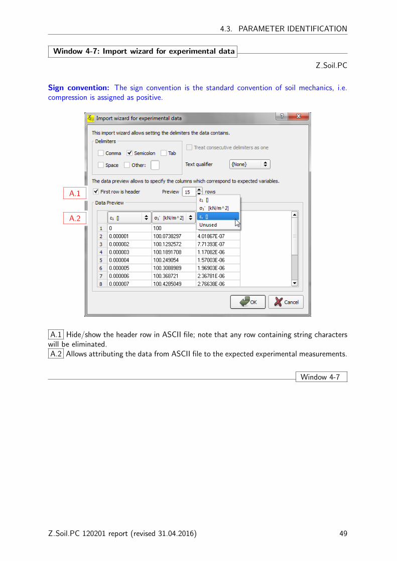
Sign convention: The sign convention is the standard convention of soil mechanics, i.e.compression is assigned as positive.

A.1

A.2

A.1 Hide/show the header row in ASCII file; note that any row containing string characterswill be eliminated.A.2 Allows attributing the data from ASCII file to the expected experimental measurements.

Window 4-7



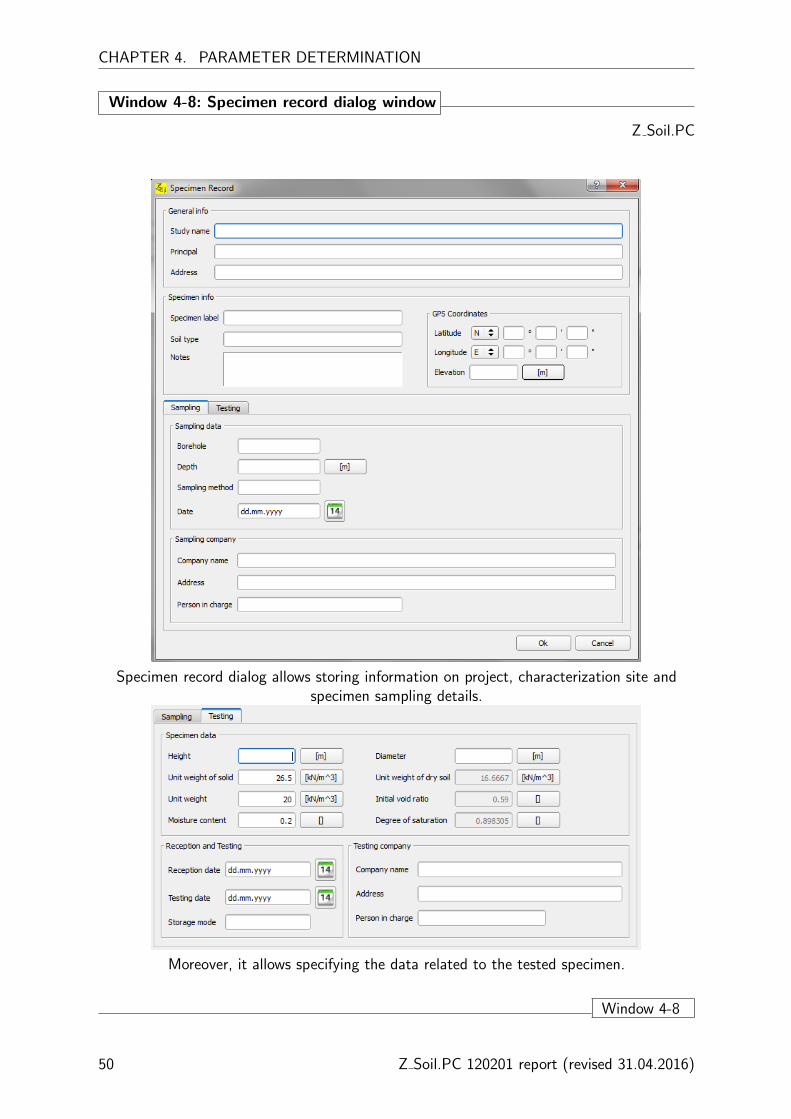
Window 4-8: Specimen record dialog window

Z Soil.PC

Specimen record dialog allows storing information on project, characterization site andspecimen sampling details.

Moreover, it allows specifying the data related to the tested specimen.

Window 4-8



Window 4-9: Data interpretation

Z Soil.PC

A.1

A.2

A.3

B.1

B.2

C.1

C.2

C.3

C.4C.5

D.1

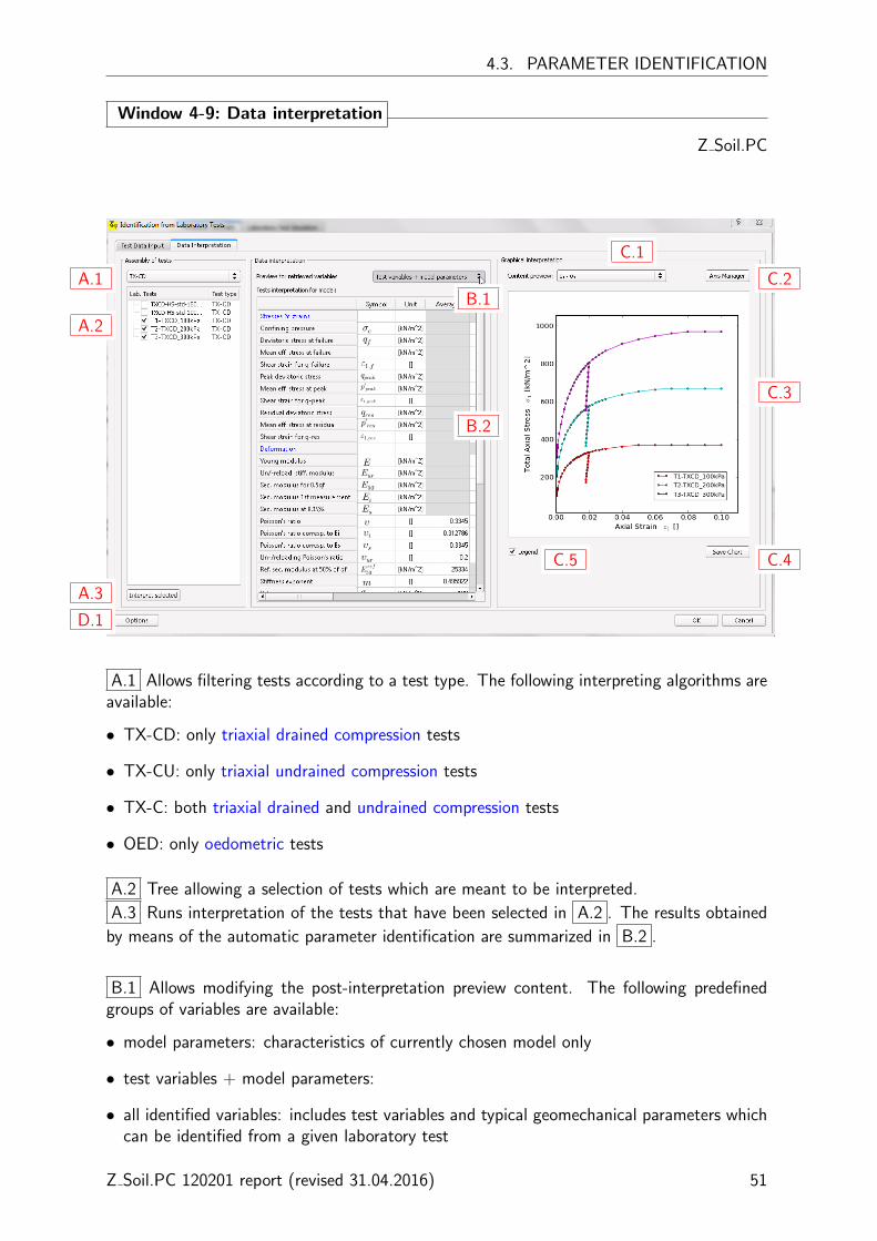
A.1 Allows filtering tests according to a test type. The following interpreting algorithms areavailable:

• TX-CD: only triaxial drained compression tests

• TX-CU: only triaxial undrained compression tests

• TX-C: both triaxial drained and undrained compression tests

• OED: only oedometric tests

A.2 Tree allowing a selection of tests which are meant to be interpreted.

A.3 Runs interpretation of the tests that have been selected in A.2 . The results obtained

by means of the automatic parameter identification are summarized in B.2 .

B.1 Allows modifying the post-interpretation preview content. The following predefinedgroups of variables are available:

• model parameters: characteristics of currently chosen model only

• test variables + model parameters:

• all identified variables: includes test variables and typical geomechanical parameters whichcan be identified from a given laboratory test



NB. Note that the experimental curves tests are interpreted with the reference to all availableinformation that experimental data may contain. Hence, any change of the constitutivemodel does not require additional reinterpretation of experimental data.

B.2 Contains results of a parameter identification run. Note that minimal and maximalvalues of parameters, as well as the standard deviation can be viewed in the tooltip by restingthe mouse cursor over the average parameter value.

C.1 Contains a number of predefined data previews.


C.3 Preview of the experimental data for the tests selected in A.2 .


C.5 Show/hide the legend in C.3 . The legend box is draggable.

D.1 Allows configuring parameter identification algorithms.

Window 4-9



Window 4-10: Configuring parameter identification

Z Soil.PC

A.1

A.2

A.3

A.1 All identified stiffness characteristics will be scaled to the defined reference stress usingthe power stiffness dependency law.

A.2 In general, different values of stiffness exponent m can be obtained in laboratory test.The user can specify stiffness characteristics based on which the stiffness exponent will beidentified.

A.3 The Young’s modulus defines the linear elastic domain in the models such as Mohr-Coulomb or Cap. Typically Young’s modulus (also called the ’static’ modulus) is identifiedthrough the triaxial test results for the axial strain equal to 0.1%. The user can modify thedefault value.

Window 4-10




Z Soil.PC

B.1

B.2

B.3

B.1 This option allows the user to decide which stresses will be used to define the failurecriterion in case of models without softening. The failure criterion is described by φf and cf .

B.2 Allows the user to specify the cycle from which the unloading-reloading modulus isidentified. Typically, the first cycles are more relevant as the specimen is subject to smalleramplitudes of shear strain and smaller non-homogeneity of stress distribution in the specimen.

B.3 Activates optimization of E50 while running the parameter identification. Note thatidentification of E50 can be affected by the volumetric plastic strains in the case of a normally-and lightly consolidated specimens.

Window 4-11




Z Soil.PC

C.1

C.2

C.3

C.4

C.5

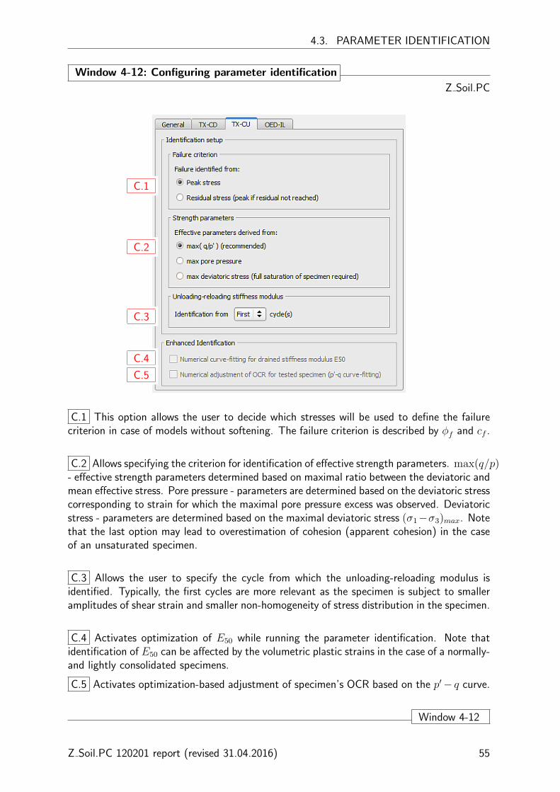
C.1 This option allows the user to decide which stresses will be used to define the failurecriterion in case of models without softening. The failure criterion is described by φf and cf .

C.2 Allows specifying the criterion for identification of effective strength parameters. max(q/p)- effective strength parameters determined based on maximal ratio between the deviatoric andmean effective stress. Pore pressure - parameters are determined based on the deviatoric stresscorresponding to strain for which the maximal pore pressure excess was observed. Deviatoricstress - parameters are determined based on the maximal deviatoric stress (σ1−σ3)max. Notethat the last option may lead to overestimation of cohesion (apparent cohesion) in the caseof an unsaturated specimen.

C.3 Allows the user to specify the cycle from which the unloading-reloading modulus isidentified. Typically, the first cycles are more relevant as the specimen is subject to smalleramplitudes of shear strain and smaller non-homogeneity of stress distribution in the specimen.

C.4 Activates optimization of E50 while running the parameter identification. Note thatidentification of E50 can be affected by the volumetric plastic strains in the case of a normally-and lightly consolidated specimens.

C.5 Activates optimization-based adjustment of specimen’s OCR based on the p′− q curve.

Window 4-12




Z Soil.PC

D.1

D.2

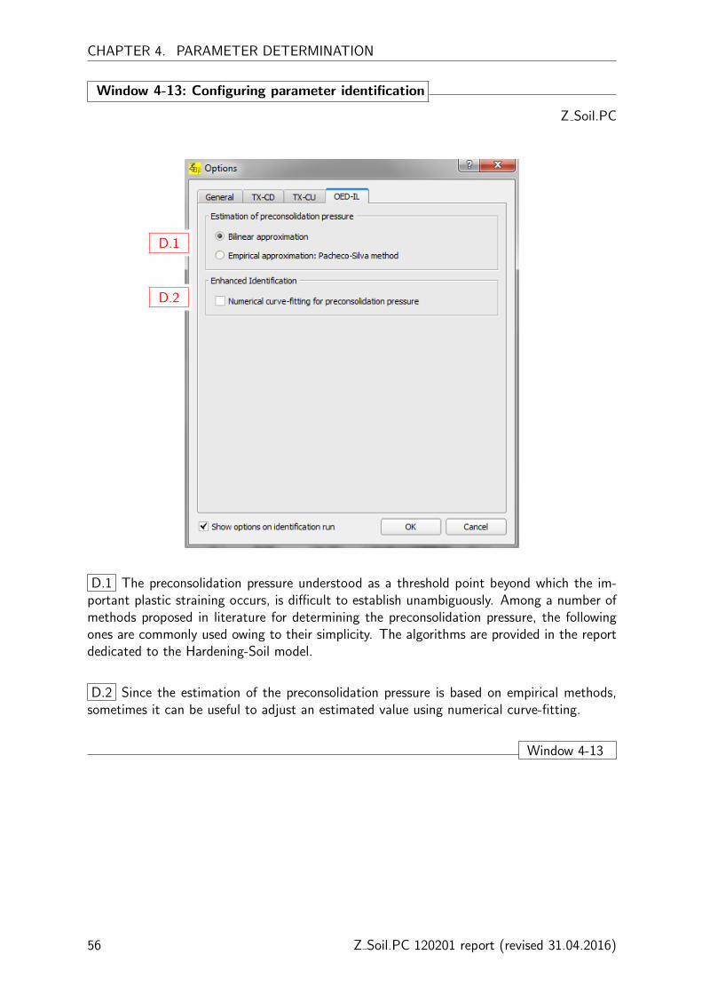
D.1 The preconsolidation pressure understood as a threshold point beyond which the im-portant plastic straining occurs, is difficult to establish unambiguously. Among a number ofmethods proposed in literature for determining the preconsolidation pressure, the followingones are commonly used owing to their simplicity. The algorithms are provided in the reportdedicated to the Hardening-Soil model.

D.2 Since the estimation of the preconsolidation pressure is based on empirical methods,sometimes it can be useful to adjust an estimated value using numerical curve-fitting.

Window 4-13


Chapter 5

PARAMETER VERIFICATION ANDVALIDATION

The laboratory test simulator offers a possibility of parameter verification and validationby running numerical simulations of elementary laboratory tests in order to visualize theconstitutive model response for the user-defined or identified model parameters.

The constitutive model can be verified for the user-defined or estimated parameters by sim-ulating one of the following elementary laboratory tests (Window 5-3):

• triaxial drained compression (TX-CD)

• triaxial undrained compression (TX-CU)

• oedometric curves (OED)

Note that no parameter determination is required to test (verify) a vector of parameters forthe constitutive model.

Model parameters which are identified based on laboratory curves can be validated by runningnumerical simulations and comparing numerical results with the laboratory curves (Window5-2). In order to compare laboratory curves with the model response, the laboratory resultshas to be imported by means of the Parameter Identification module.

CHAPTER 5. PARAMETER VERIFICATION AND VALIDATION

Window 5-1: Calling the Laboratory Test Simulator

Z Soil.PC

The Laboratory test simulator can be called by pressing Lab Test Simulation.

Window 5-1


Window 5-2: Validation of model parameters

Z Soil.PC

A.1

A.2

A.3

A.4

A.5

B.1

B.2

B.3 B.4

C.1 C.2

C.3

C.4

C.5

A.1 Allows filtering tests according to the test type. The test simulation can be run in

order to evaluate model behavior to the specified vector of parameters B.2 or to comparemodel response with experimental data. The following elementary laboratory tests can besimulated:

• TX-CD: strain-controlled, one-element triaxial drained compression; analysis type Axisymmetry,problem type Deformation, driver type Driven Load

• TX-CU: strain-controlled, one-element triaxial undrained compression; analysis type Axisymmetry,problem type Deformation+Flow, driver type Driven Load (Undrained)

• OED-IL: stress-controlled , one-element oedometric compression; analysis type Axisymmetry,problem type Deformation+Flow, driver type Driven Load

A.2 Show the assembly of real tests which have been specified in Test data input.

A.3 Allows a selection of tests which are meant to be simulated.

A.4 Run a numerical simulation for the selected test using initial state variables from B.1

and vector of parameters B.2 . The results will be presented in C.3 .

A.5 Run simulation of all checked tests. The results will be presented in C.3 for the se-lected tests.

B.1 Preview of initial state variables for currently selected test only. Since the initial statevariables are specified in Test data input, the values are not editable.B.2 Allows specifying model parameters. Note that these parameters can be automatically



imported from parameter summary widget.B.3 Allows importing model parameters from the ”User’s selection” or those obtained by

determination methods.B.4 Allows sending the whole vector of modified parameter values to the ”User’s selection”.

Sign convention: The sign convention is the standard convention of soil mechanics, i.e.compression is assigned as positive.C.1 Contains a number of predefined data previews.


C.3 Preview of experimental data and results obtained by means of a numerical simulation.


C.5 Control the simulation status and the log of computations.

Window 5-2


Window 5-3: Verification of model parametersZ Soil.PC

A.1

A.2

A.3

A.4

B.1

B.5

B.3 B.4

B.2

C.1 C.2

C.3

C.4

C.5

A.1 Cf. Window 5-2.

A.2 Deactivation of real test data.

A.3 Allows a selection of tests which are meant to be simulated.

A.4 Run a numerical simulation for the selected test using initial state variables from B.1

and vector of parameters B.6 . The results will be presented in C.3 .

B.1 Allows specifying initial state variables for currently selected test.

B.2 Allows defining/modifying model parameters.

B.3 Cf. Window 5-2.

B.4 Cf. Window 5-2.

B.5 Allows specifying a customizedloading program. Note that unwanted rows in the load-ing program can me removed by clicking the right-click button over the first column of theunwanted row.

Sign convention: The sign convention is the standard convention of soil mechanics, i.e.compression is assigned as positive.C.1 Cf. Window 5-2

C.2 Cf. Window 5-2

C.3 Cf. Window 5-2

C.4 Cf. Window 5-2

C.5 Cf. Window 5-2

Window 5-3


Chapter 6

PROJECT AND DATAMANAGEMENT

Window 6-1: Dialog on the toolbox exit

Z Soil.PC

A.1

A.2

A.1 All inserted or modified data will be saved in a file [current-project-name].pid

A.2 All cells will be updated in main Material dialog

Window 6-1

CHAPTER 6. PROJECT AND DATA MANAGEMENT

Window 6-2: Format of saved data

Z Soil.PC

The project is saved in the easily accessible xml data format.

• project: [current-project-name].pid

• single laboratory test: [test-name].pit

Window 6-2


REFERENCES

Bowles, J. (1997). Foundation analysis and design. McGraw-Hill. 32

Campanella, R., Robertson, P., and Gillespie, D. (1986). Seismic cone penetration test. InClemence, S., editor, In Situ’86: Use of In-situ in Geotechnical Engineering, ASCE, volumeGSP6, pages 116–130, Blacksburg, VA. ASCE. 33

Liao, S. and Whitman, R. (1986). Overburden correction factors for. spt in sand. J GeotechEng ASCE, 112(3):373–377. 32

Long, M. (1998). Design parameters from in situ tests in soft ground - recent developments.pages 363–372. 33

Lunne, T., Robertson, P., and Powell, J. (1997). Cone penetration testing in geotechnicalpractice. Blackie Academic & Professional, London. 25, 26

Mair, R. and Wood, D. (1987). Pressuremeter testing. Methods and interpretation. Butter-worths, London. 29

Marchetti, S. (1980). In situ tests by flat dilatometer. J Geotech Eng ASCE, 106(3):299–321.27, 28

Marchetti, S. and Crapps, D. (1981). Flat dilatometer manual. Technical report. 28

Marchetti, S., Monaco, P., Totani, G., and Calabrese, M. (2001). The flat dilatometer test(dmt) in soil investigations. In TC16, I. C., editor, IN SITU 2001, Int Conf On In situMeasurement of Soil Properties, Bali. ISSMGE. 27

Marchetti, S., Monaco, P., Totani, G., and Marchetti, D. (2008). In situ tests by seismicdilatometer (sdmt). ASCE Geot. Special Publication, GSP170:292–311. 33

Robertson, P. (1990). Soil classification using the cone penetration test. Can Geotech J,27(1):151–158. 25, 26

Robertson, P. and Cabal, K. (2010). Guide to cone penetration testing for geotechnicalengineering. 4th edition. Technical report, Gregg Drilling and Testing, Inc. 26

van Genuchten, M. (1980). A closed-form equation for predicting the hydraulic conductivityof unsaturated soils. Soil Sci. Soc. Am. J, 44:892–898. 3

Yang, H., Rahardjo, H., Leong, E., and Fredlund, D. (2004). Factors affecting drying andwetting soil-water characteristic curves of sandy soils. Can Geotech J, 41:908–920. 3

virtual lab - zsoil · virtual lab z soil.pc 120201 report revised 15.04.2016 by ... p.o.box 224,...

Documents