Virtual Constraint Control of a Powered Prosthetic Leg:From Simulation to Experiments with Transfemoral Amputees

Robert D. Gregg, Member, IEEE, Tommaso Lenzi, Member, IEEE, Levi J. Hargrove, Member, IEEE, andJonathon W. Sensinger, Member, IEEE

Abstract—Recent powered (or robotic) prosthetic legsindependently control different joints and time periods of thegait cycle, resulting in control parameters and switching rulesthat can be difficult to tune by clinicians. This challenge mightbe addressed by a unifying control model used by recent bipedalrobots, in which virtual constraints define joint patterns asfunctions of a monotonic variable that continuously representsthe gait cycle phase. In the first application of virtual constraintsto amputee locomotion, this paper derives exact and approximatecontrol laws for a partial feedback linearization to enforce virtualconstraints on a prosthetic leg. We then encode a human-inspiredinvariance property called effective shape into virtual constraintsfor the stance period. After simulating the robustness of thepartial feedback linearization to clinically meaningful conditions,we experimentally implement this control strategy on a poweredtransfemoral leg. We report the results of three amputee subjectswalking overground and at variable cadences on a treadmill,demonstrating the clinical viability of this novel control approach.

I. INTRODUCTION

Amputee locomotion is slower, less stable, and requiresmore metabolic energy than able-bodied locomotion [1]–[3].Individuals with lower-limb amputations fall more frequentlythan able-bodied individuals and often struggle to navigateramps, hills, and stairs [2]. These challenges can be attributedlargely to the use of mechanically passive prosthetic legs [3],which do not actively respond to perturbations or contributepositive work as do the muscles in biological legs. Recentpowered legs could significantly improve mobility and qualityof life for millions of lower-limb amputees, but controlchallenges currently limit the clinical viability of these devices.

With the addition of sensors and motors, powered prostheticlegs must continuously make control decisions throughoutthe gait cycle, thus increasing the complexity of thesedevices. Control engineers typically handle this complexity

Asterisk indicates corresponding author.R. D. Gregg* is with the Departments of Bioengineering and Mechanical

Engineering, University of Texas at Dallas, Richardson, TX 75080 USA.rgregg@ieee.org

T. Lenzi and L. J. Hargrove are with the Center for Bionic Medicine,Rehabilitation Institute of Chicago and the Department of Physical Medicine& Rehabilitation, Northwestern University, Chicago, IL 60611 USA.

J. W. Sensinger is with the Institute of Biomedical Engineering andDepartment of Electrical and Computer Engineering, University of NewBrunswick, Fredericton, NB E3B 9P8, Canada. sensinger@ieee.org

This research was supported by USAMRAA grant W81XWH-09-2-0020. R.D. Gregg holds a Career Award at the Scientific Interface from the BurroughsWellcome Fund. This work was also supported by the National Instituteof Child Health & Human Development of the NIH under Award NumberDP2HD080349. The content is solely the responsibility of the authors anddoes not necessarily represent the official views of the NIH.

by discretizing the gait cycle into multiple time periods1, eachhaving its own separate control model [4]–[7]. The prevailingmethodology also controls each joint independently in multi-joint prostheses [5], [6]. Each control model may enforcedesired impedances (i.e., joint stiffness and viscosity [4], [5])or track pre-defined patterns of joint angles [8], [9], velocities[10], or torques [7], [11]. These prosthetic legs switch betweencontrol models based on switching rules or estimates of gaitcycle phase that rely on multiple sources of sensory feedback.

This approach to prosthetic leg control has two keychallenges: 1) reliability of the phase estimate for switchingcontrol models and 2) difficulty of tuning control parametersfor several control models to each joint, patient, and task. Anerror in the phase estimate can cause the prosthesis to enact thewrong control model at the wrong time, potentially causing thepatient to fall. Moreover, each control model must be carefullytuned by a team of clinicians and researchers to work correctlyfor a particular patient performing a particular task [6]. Someprosthetic control systems have five discrete periods of gaitwith more than a dozen control parameters per joint per period[5]. Although recent methods attempt to automate the tuningof these parameters [6], multiple tasks (e.g., walking, standing,and stair climbing) add up to hundreds of parameters for multi-joint prosthetic legs. The goal is therefore to minimize thenumber of control switches and hand-tuned parameters.

This goal could potentially be achieved by parameterizinga nonlinear control model with a mechanical representation ofthe gait cycle phase, which could be continuously measuredby a prosthesis to match the body’s progression through thecycle. This idea originates from recent work in autonomousbipedal robots, which can walk, run, and climb stairs usinga control framework known as partial feedback linearization2

[12]. This geometric control approach produces joint torquesto virtually enforce kinematic constraints, which define desiredjoint patterns as functions of a mechanical phase variable(e.g., hip position). Although experiments with bipedal robotsincluding [12]–[16] demonstrate the exceptional performanceenabled by virtual constraints, this control approach has neverbeen applied to the field of prosthetics. The closest knownapproach [9] tracks a pre-recorded human ankle trajectorybased on a mechanical phase variable, but data-driven patternsmay not generalize to different users, tasks, or joints as easilyas symbolic virtual constraints defined from a minimal setof tunable parameters. Prosthetic virtual constraints could

1These discrete periods of gait are commonly called ‘phases,’ but we avoidthis nomenclature to avert confusion with our continuous definition of phase.

2The feedback linearization is called ‘partial’ because only the input-outputdynamics are linearized, whereas the internal dynamics may remain nonlinear.

coordinate multi-joint patterns across different periods of gait,measuring a phase variable to match human motion as opposedto methods relying on feedback from the sound leg [8], [17].

The application of virtual constraints to prostheticsraises new theoretical challenges related to partial feedbacklinearization with human-machine interaction, such as thepresence of interaction forces and the lack of state feedbackfrom the human body. We recently derived a linearizingcontroller for a prosthetic ankle using only feedback availableto sensors on the prosthesis [18], but this strategy did notinclude the knee joint for transfemoral (above-knee) amputees.We extended virtual constraints to the knee joint and simulatedthis coordinated control strategy in [19]. These simulationsmotivated pilot experiments with a powered prosthetic leg in[20], where the prosthesis was attached to the thigh of an able-bodied subject through a leg-bypass adapter. These preliminaryworks did not, however, demonstrate the clinical viability ofthe control strategy with amputee patients.

This paper employs the method of virtual constraintson a powered prosthetic leg to unify the stance period,coordinate ankle and knee control, and accommodate clinicallymeaningful walking conditions in both simulations andexperiments with transfemoral amputee subjects. Becauseamputees often struggle to adapt to varying conditions like gaitspeed and shoe geometry [2], we employ the invariant propertyof effective shape (or rollover shape) as a virtual constraint.An effective shape is the trajectory of the center of pressure(COP)—the location of the ground reaction force under thefoot—mapped into a moving reference frame attached tothe stance leg [21]. From the perspective of the leg, theCOP stays on an effective shape that is invariant over gaitspeeds [22], heel heights [23], shoe curvatures [24], and bodyweights [21], suggesting that a prosthetic leg could naturallyaccommodate these conditions by enforcing the effectiveshape. We therefore model two effective shapes as virtualconstraints that parameterize the stance period with the heel-to-toe movement of the COP as a phase variable.

We begin with the theory of virtual constraints for aprosthetic leg in Section II, extending the preliminary works[18], [19] by defining both exact and approximate feedbacklinearizations for general constraint functions before modelingthe effective shapes. In Section III we model the hybrid systemof an amputee biped with prosthetic legs controlled by virtualconstraints during stance and joint impedance during swing.Going beyond the case of exact feedback linearization in [19],the simulations in Section IV demonstrate the robustness of thevirtual constraints to variable walking conditions, approximatefeedback linearization, and noisy phase measurements. Thesesimulations motivate the experimental implementation inSection V, where we report the results of three transfemoralamputee subjects walking overground and at variable cadenceson a level treadmill. All three subjects achieved stable walking(Fig. 1) after minimal tuning of a small set of parameters. Wediscuss these results and limitations of the study in SectionVI, and we conclude in Section VII.

Fig. 1. Images of transfemoral amputee subject walking on the Vanderbiltprosthetic leg (designed in [5]) using the proposed virtual constraint strategy.

𝑚s

−𝜃h

𝛾

𝑅f

(𝑞𝑥, 𝑞𝑧)

𝐶𝑂𝑃

𝑃f

𝐹𝑥

𝜙 𝜃a

−𝜃k 𝑚t

−𝐹𝑧

𝑚h 𝑚t

𝜃sk

−𝜃sa

𝑚s

𝑚f

ℓt

ℓf

ℓs

𝑥

𝑀𝑦

𝑧

Fig. 2. Kinematic model of transfemoral amputee biped, where the prostheticstance leg is shown in solid gray and the body in dashed black. The lengthsof the heel, shank, and thigh segments are labeled `f , `s, and `t, respectively.The radius of curvature Rf and center of rotation Pf define the rocker footgeometry. Dorsiflexion/plantarflexion of the stance ankle and extension/flexionof the stance knee are defined in the positive/negative directions.

II. VIRTUAL CONSTRAINTS FOR A PROSTHETIC LEG

We now present a prosthetic control framework that iscapable of unifying certain periods of the gait cycle throughthe use of virtual constraints. After deriving both an exact andan approximate control law for general virtual constraints, wespecifically employ the invariance property of effective shapeto 1) unify the stance period, 2) coordinate multi-joint control,and 3) enable the prosthesis to accommodate variations incadence, shoe geometry, and body mass.

A. Modeling the Prosthesis

The prosthetic leg depicted in Fig. 2 (solid gray) is attachedto the hip of the body, which is shown in dashed black. Wefirst model the prosthetic leg for our control derivation in thissection and return to the full biped model in Section III forthe purpose of simulation in Section IV.

1) Dynamics: We model the prosthetic leg as a kinematicchain with respect to an inertial reference frame attached tothe ground (Fig. 2). We define a floating coordinate frame at

the prosthetic heel, treating its position coordinates (qx, qz) asstate variables that will later be constrained by a contact model.The full configuration of the leg in configuration space Q =R2×T3 is given by q = (qx, qz, φ, θa, θk)T , where φ is the footorientation with respect to vertical, θa is the ankle angle, andθk is the knee angle. The state of the dynamical system is thengiven by vector x = (qT , qT )T ∈ TQ, where q ∈ R5 containsthe joint velocities. The state trajectory evolves according toa differential equation of the form

M(q)q + N(q, q) +A(q)Tλ = Bu+ J(q)TF (1)

where M ∈ R5×5 is the inertia/mass matrix, N ∈ R5

is a vector that groups the Coriolis/centrifugal terms andgravitational forces, A ∈ Rc×5 is the matrix modeling cphysical constraints between the foot and ground, and λ ∈ Rcis the Lagrange multiplier used to calculate the contact forces.

The external forces on the right-hand side of (1) respectivelycomprise actuator torques and interaction forces with the body.Ankle and knee actuation from torque input u ∈ R2 is mappedinto the leg’s coordinate system by B = (02×3, I2×2)T ∈R5×2. The interaction force F = (Fx, Fz,My)T ∈ R3 at thesocket—the connection between the prosthesis and body at thehip in Fig. 2—comprises two linear forces and a moment inthe sagittal plane [25], which can be measured by a 3-axisload cell at the socket. Force vector F acts at the end-point ofthe leg’s kinematic chain and is mapped to joint torques/forcesby the body Jacobian matrix J(q) ∈ R3×5, which we modelusing the standard procedure in [26].

2) Stance Period: During the prosthesis stance periodwe must model the physical forces associated with contactbetween the prosthetic foot and ground. These contact forcesprevent the foot from slipping and falling through the ground,which constitute at least two physical constraints on dynamics(1). Therefore, foot geometry is commonly modeled (e.g.,[12]–[15], [27]) as a vector holonomic constraint

a(q) = 0, (2)

where a : Q → Rc for c ≥ 2. In Section III we will employthe rocker feet seen in Fig. 2, but other geometries such as flatfeet [28], [29] could similarly be modeled in this framework.

Given contact constraint a(q) = 0, we follow the method in[26] to compute the constraint matrix A = ∇qa and Lagrangemultiplier λ = λ+λu+λF , where (omitting matrix arguments)

λ = W (Aq −AM−1N), (3)

λ = WAM−1B, λ = WAM−1JT

for W = (AM−1AT )−1. These terms enter into dynamics (1)only during the stance period of the prosthetic leg.

3) Swing Period: During the swing period of the prosthesis,the prosthetic foot is not in contact with the ground, so nocontact constraints are invoked in the prosthesis dynamics, i.e.,λ = 0 in (1). Although the prosthesis is still modeled withrespect to its heel point, the interaction force F in prosthesisdynamics (1) suspends the prosthetic leg from the body’s hip.

B. Definition of a Virtual Constraint

Although defined in a similar manner to physical/contactconstraints, virtual constraints are enforced by actuator torquesrather than external physical forces. The vast majority ofvirtual constraints used in bipedal robots are holonomic [12]–[16], so we translate these design principles into our prostheticframework by considering virtual holonomic constraints

h(q) = 0, (4)

where h : Q → R2 for an actuated knee and ankle, i.e., onevirtual constraint per actuated degree-of-freedom (DOF).

Remark 1: Meaningful virtual constraints, i.e., outputfunctions h(q), can be defined in a variety of ways. Reviewingprevious work in bipedal robotics (e.g., [12], [13], [15]), virtualconstraints can be used to control the actuated joints specifiedby h0(q) = (θa, θk)T to a desired trajectory hd(Θ(q)) ∈ T2 asa function of a monotonic quantity Θ(q) ∈ R. This quantity,known as the phase variable or timing variable, provides aunique representation of the gait cycle phase to drive forwardthe desired pattern in a time-invariant manner. In this case,the output function of equation (4) would be defined byh(q) = h0(q) − hd(Θ(q)). The desired pattern hd can bedefined first as a function of time (via boundary-constrainedoptimization) and then re-parameterized into a function ofΘ(q) [12]. We will see that h(q) can also be defined directlyfrom geometric relationships found in human walking, withoutspecifying a desired angular trajectory.

Given desired virtual constraints (4), the goal of a virtualconstraint controller is to drive output function h(q) to zero.Therefore, the control system output

y := h(q) (5)

corresponds to tracking error from the desired constraint (4).Some torque control methods are better suited than others

at driving this output to zero. If we do not start with a desiredjoint pattern hd (Remark 1), it is not always possible to solvea virtual constraint (4) for a unique joint trajectory as neededfor joint impedance methods [4]–[7]. Bipedal robots typicallyenforce virtual constraints using partial (i.e., input-output)feedback linearization [12], which has appealing theoreticalproperties including exponential convergence [30], reduced-order stability analysis [12], and robustness to model errors[13]. However, the application of this method to prostheticspresents unique challenges with human-machine interaction.

C. Partial Feedback Linearization of the Prosthesis

We cannot expect to have either a model of the humanor sensors at intact joints in a clinically viable system. Thecontroller should then rely only on the prosthesis model, i.e.,terms in (1), and feedback available to onboard sensors, i.e.,state x = (qT , qT )T and interaction force F . The lack of fullstate feedback from the biped system presents a challenge notpreviously encountered in implementations of partial feedbacklinearization on bipedal robots [13]. Therefore, in this sectionwe show that measurements of interaction force F will allowus to achieve similar results on a prosthetic leg.

As previously stated, our goal is to define a feedback controllaw for input u that drives output y to zero in dynamics (1). Aninput-output linearizing control law is derived in [19] using Liederivative notation from [30], but for clarity here we derive anequivalent control law in terms of the matrices in (1). We startby examining the first-order output dynamics y = (∇qh)q.Because the control input u does not appear in these dynamics,output y has relative degree greater than one (cf. [30]) andanother time-derivative is needed to expose the control input.Letting H := ∇qh, the second-order output dynamics are

y = Hq +Hq

= Hq +HM−1(−N −ATλ+Bu+ JTF )

= Hq −HM−1(N +AT λ) +HM−1(B −AT λ)u

+ HM−1(JT −AT λ)F. (6)

The output function y = h(q) can be chosen such that the2× 2 decoupling matrix

D(q) := HM−1(B −AT λ)

= HM−1(I −ATWAM−1)B (7)

is non-singular over feasible walking configurations, whichcan be verified numerically. We can then solve for the controllaw that inverts the output dynamics (6):

ulinz := D−1[−Hq +HM−1(N +AT λ)

−HM−1(JT −AT λ)F + upd]. (8)

Defining a proportional-derivative (PD) input

upd := −Kpy −Kdy (9)

with positive-definite Kp,Kd ∈ R2×2, control law (8) rendersthe output dynamics (6) linear and exponentially stable:

y = upd = −Kpy −Kdy. (10)

Remark 2: The linear output dynamics (10) imply y(t)→ 0exponentially fast as t → ∞ for y(0) 6= 0. The feedbacklinearization provides y ≡ 0 in steady-state, implying thatthe surface Z = {x | y = 0, y = 0} is invariant3 underthe closed-loop continuous dynamics. This allows system(1) to be restricted to lower-dimensional zero dynamics onsurface Z, where holonomic virtual constraints provide greaterdimensionality reduction than nonholonomic constraints [12],[30]. The holonomic outputs characterize the two actuatedDOFs, whereas the zero dynamics represent the unactuatedDOFs (qx, qz, φ) coupled with the human through interactionforce F . These lower-dimensional dynamics determine thecontinuous behavior of the full system (1) through the virtualconstraints. Classical results in [30] can be invoked to showthat the full system is stable if the zero dynamics are stableunder control law (8). However, walking has discontinuousimpact events (Section III), so surface Z may not be hybridinvariant, i.e., y = 0 immediately before heel strike may notimply y = 0 immediately after heel strike. We will see inSection IV that the PD terms in (10) quickly correct errors

3Any state trajectory initialized on an invariant surface of a continuoussystem will remain on the surface for all time [30].

from impacts, by which we approximate hybrid zero dynamicsto provide stability of the full hybrid system (cf. [12]). We willexploit the existence of passive gaits down shallow slopes [31]to stabilize the hybrid zero dynamics (and therefore the fullhybrid system) in the simulations of Section IV. Similarly, thehuman wearing the prosthesis will help stabilize the hybridzero dynamics in the experiments of Section V.

The zero dynamics on Z are defined by the virtualconstraints, independent of the control law enforcing them(and other methods exist, e.g., finite-time control [12], inversedynamics [29], and control Lyapunov functions [32]). We nowpresent a simpler control law that approximates this partialfeedback linearization for our experimental implementation.

D. Approximation of the Partial Feedback Linearization

Although this partial feedback linearization has manybeneficial properties, control law (8) can be difficult toimplement in practice. Its dependence on interaction forceF requires a 3-axis load cell at the socket. This controllaw also requires an accurate dynamical model (1) of theprosthesis, which could present a barrier to clinical viabilitywhen components like prosthetic feet are interchangeable.

We can avoid these potential limitations, while stillleveraging the theoretical results of Remark 2, byapproximately enforcing virtual constraints with the linearpart (9) of control law (8). With sufficiently large PD gains inmatrices Kp,Kd, the linear terms will dominate the nonlinearterms in (8). We therefore approximate the exact controllaw ulinz using only the output PD control law upd. Virtualconstraints are typically implemented in this approximatemanner on experimental bipedal robots [12]–[15].

Remark 3: If the decoupling matrix D(q) is positive-definiteand the PD gains are sufficiently large, the outputs will remainclose to zero in the output dynamics (6) under control law(9). The prosthesis dynamics (1) will then be close to thezero dynamics in Remark 2, providing a lower-dimensionalsystem for the human-in-the-loop to stabilize. Alternatively,the human interaction force in (6) may help enforce the virtualconstraints, allowing the use of small gains in controller (9)as we will see in Section V.

Although control law (9) is linear in the outputs, theseoutputs are typically nonlinear functions of configuration q,e.g., the phase variable Θ(q). In the next section we willchoose these nonlinear functions such that their dependenceon a phase variable allows a prosthetic leg to perform phase-specific behaviors that mimic able-bodied human gait.

E. Choosing the Virtual Constraints

The goal of this paper is to implement virtual constraintsthat unify the stance period, coordinate ankle and kneecontrol, and accommodate clinically meaningful conditionson a powered prosthetic leg. For this purpose we employa geometric relationship of the stance leg that is invariantacross walking conditions including gait speed, shoe geometry,and body weight [21]. This invariance property, known as theeffective shape in the prosthetics field, is often used as a metric

Fig. 3. Diagrams of the ankle-foot (left) and knee-ankle-foot (right) effectiveshapes. The COP moves along each shape (dashed curve) in the shank-basedor thigh-based coordinate frame (solid axes).

for aligning passive prostheses [33]. We define the effectiveshape and show that it can be treated as a virtual holonomicconstraint with certain assumptions about the stance contactmodel—the swing period is considered later.

1) Definition of Effective Shape: Reviewing the preliminaryworks [19] and [20], an effective shape characterizes howthe stance leg joints move as the COP travels from heel totoe. Able-bodied humans have effective shapes specific toactivities such as walking [21], stationary swaying [34], andstair climbing [35], and each shape can be characterized bythe curvature of the COP trajectory with respect to a referenceframe attached to the stance leg. In particular, the ankle-foot (AF) effective shape is the COP trajectory mapped intoa shank-based reference frame (axes xs, zs in Fig. 3, left),and the knee-ankle-foot (KAF) effective shape is the COPtrajectory mapped into a thigh-based reference frame (axesxt, zt in Fig. 3, right). These leg-based frames share an originat the ankle, but zs is attached to the knee and zt to the hip.

These two shapes can be modeled by the distance betweenthe COP and a point Pi = (Xi, Zi)

T attached to the respectiveleg-based reference frame:

||Pi − COP || = Ri, i ∈ {s, t}, (11)

where the radius of curvature Ri is approximately constantwithin standing or walking tasks [34]. These two effectiveshapes provide two virtual constraints to control two joints—the ankle and knee of the prosthesis.

2) Effective Shape as a Virtual Holonomic Constraint:In order to employ these effective shapes in the linearizingcontrol law (8), equation (11) must be expressed as aholonomic constraint in the coordinates of our leg model.This requires the COP to be a function of the configuration q,despite the fact that the COP is usually expressed as a functionof forces [36]. We can treat the COP as a position variable ifwe assume rolling point contact between the foot and ground,which can be achieved with a rocker foot as depicted in Fig. 2.This modeling assumption originates from works showing thatrocker feet are suitable substitutes for compliant feet, whichare difficult to model, when simulating human-like dynamic

walking [27], [37] and when designing prosthetic feet [38].This contact model is defined in Section III-B and AppendixA, and its limitations are discussed in Section IV-E.

We can now express the vector from the COP to the centerof rotation Pi as a function PCOPi (q), i ∈ {s, t}, as defined inAppendix B. Equation (11) is then given in model coordinatesby the kinematic constraint hi(q) = 0 for

hi(q) := Ri − norm(PCOPi (q)), i ∈ {s, t}. (12)

This function is the output of a virtual constraint, whichcorresponds to the distance from the desired effective shape.Hence, the vector output of the AF and KAF virtual constraintsis defined as y := h(x) = (hs(x), ht(x))T .

Remark 4: These effective shapes are virtually enforced ona prosthetic leg by driving output y to zero, which can beachieved exactly using control law (8) or approximately using(9). Virtual constraints (12) depend on the COP, which movesmonotonically from heel to toe during steady walking. Thischoice of constraints should then synchronize the knee andankle patterns through their mutual dependence on the COPas a phase variable, i.e., Θ(q) = qx in Remark 1.

Because an effective shape is not defined for the swing leg(which has no COP), we will instead control the swing periodwith the clinically familiar concept of joint impedance—thestiffness and viscosity of a joint—which is the current standardfor controlling powered prosthetic limbs [5]–[7]. We will usejoint PD control for this purpose in Sections III–V. Ourfeedback linearization approach could be used during swingwith another choice of virtual constraints, but in this paperwe focus on the stance period as a starting point for the firstapplication of this theory to a prosthetic leg.

Now that we have derived an exact and an approximatepartial feedback linearization for clinically-motivated virtualconstraints, we should validate the feasibility and analyzethe robustness of this prosthetic control strategy beforeexperimentally implementing it for amputee subjects. We willperform this analysis in simulation, requiring us to model abiped to interact with the prosthetic limb as would an amputee.

III. MODELING AN AMPUTEE BIPED FOR SIMULATION

In this section we model the amputee biped of Fig. 2 for thepurpose of simulating a prosthetic leg under virtual constraintcontrol in Section IV. These simulations require us to considerthe coupled dynamics of the body and the prosthesis for a totalof 8 DOFs. The extended configuration vector is denoted byqe = (qT , θh, θsa, θsk)T ∈ Q × T3, where θh is the body’ship angle, θsa is the swing ankle angle, and θsk is the swingknee angle. For simplicity we assume symmetry in the fullbiped (i.e., a bilateral transfemoral amputee with two identicalprosthetic legs), where each prosthesis uses the same controlstrategy. The prosthetic legs do not communicate, so eachleg interacts with the model’s hip and opposing leg throughinteraction forces in (1) as it would with a human body,whether or not the opposing leg is prosthetic.

We model a passive human hip in order to 1) test theinherent stability of the prosthesis controller without activehuman assistance and 2) avoid the impractical task of modeling

a realistic human controller. For this purpose we exploit theexistence of passive walking gaits, which arise on declinedsurfaces when the potential energy converted into kineticenergy during each step replenishes the energy dissipated atimpacts [28], [31]. This behavior reflects certain characteristicsof human gait, such as ballistic swing motion [39] andenergetic efficiency down slopes [40]. We therefore model adownhill slope condition to power the hip in these simulations.

A. Control Strategy

Although the control laws in Section II could employ virtualconstraints for both the stance and swing periods, this paperfocuses on the use of effective shape as a virtual constraint forits invariance properties during stance. Because no effectiveshape is known for the swing leg [21], we instead use thestandard method of joint PD control (often called impedancecontrol) during swing [5]. This passive method can enableballistic motion of the swing leg as in human walking [39].Because the prosthesis does not bear the user’s body weightduring the swing period, this model-free method can accuratelydrive the prosthetic joints to flexion angles needed to achievetoe clearance, which is critical to amputee locomotion.

Although the human hip joint is powered by gravity in oursimulation, we add a spring-damper to the joint for consistentstep placement. Therefore, the vector of control torques forthe entire biped (prostheses and amputee) is given by

τe = (BT , 02×3)Tust+(01×5, 1, 01×2)Tuh+(02×6, I2×2)Tusw

where ust = ulinz(x) or ust = upd(x), and the hip input uh ∈R and the swing prosthesis inputs in usw = (usa, usk)T ∈ R2

have the form

ui := −kpi(θi − θeqi )− kdiθi, (13)

where kpi, kdi, and θeqi respectively correspond to the stiffness,viscosity, and equilibrium angle of joint i ∈ {h, sa, sk}. Wesaturate the prosthesis torques at 80 N·m to simulate the torquelimit of the experimental prosthesis in Section V.

B. Hybrid Dynamics

Bipedal locomotion involves both continuous and discretedynamics, which constitute a hybrid dynamical system. Herewe summarize these hybrid dynamics from [19]. The biped’scontinuous dynamics are governed by a differential equationof the form (1). Noting that the derivation for control law (8) inSection II did not depend on a specific choice of foot contactconstraints, we must first define a contact model.

To model the biped’s contact constraints in the context ofSection II-A2, we choose constant-curvature rocker feet toapproximate the deformation of human feet during walking[27], [37]. The associated contact constraints (2) are modeledin Appendix A, where aroll1 (q) constrains coordinates qx, qzto an arc of radius Rf , and aroll2 (q) constrains φ to beperpendicular to the arc. The foot does not extend behindthe heel link in Fig. 2, so depending on orientation φ therocker may not be in contact with the ground at heel strike(qx = qz = 0). In this case the biped rotates about the heelwith constraints defined by aheel1 (q) := qx, aheel2 (q) := qz ,

which fix the heel position to the ground. These constraintsmodel physical contact, whereas the effective shapes in SectionII-E serve as virtual constraints for joint control.

Given this contact model, the constraint terms A and λin dynamics (1) are computed according to the definitionsin Section II-A2. We denote the heel contact matrix asAheel = ∇qaheel or Aeheel = ∇qeaheel and the rolling contactmatrix as Aroll = ∇qaroll or Aeroll = ∇qearoll. The modelswitches from heel contact to rolling contact when the soleintersects the ground, i.e., when aroll2 (q) = 0.

One step period then consists of a sequence of heel contactdynamics, a foot-slap impact event, rolling contact dynamics,and a ground-strike impact event with impact map ∆e:

Meqe + Ne +AeTheelλe = τe, if aroll2 (qe) 6= 0

qe+ = (I − X(AerollX)−1Aeroll)qe

−, if aroll2 (qe) = 0

Meqe + Ne +AeTrollλe = τe, if pzγ(qe) 6= 0

(q+e , qe+) = ∆e(q

−e , qe

−), if pzγ(qe) = 0

which then returns to the beginning of the sequence forthe next step [19]. Note that X = M−1

e AeTroll, superscripts

+/− respectively denote post/pre-impact, and pzγ(qe) ∈ R isthe height of the swing foot heel above ground with slopeangle γ. Extended terms are defined as in Section II withrespect to the extended configuration qe. After imposing thecontact constraints, the full biped model has one degree ofunderactuation: foot orientation φ, which is constrained to aone-to-one relationship with the COP during rolling contact.

C. Stability of Hybrid Limit Cycles

This hybrid dynamical system can be analyzed for stabilityas in [28]. Letting xe = (qTe , qe

T )T be the state vector for thefull biped, walking gaits are cyclic and correspond to solutioncurves xe(t) of the hybrid system such that xe(t) = xe(t+T )for all t ≥ 0 and some minimal T > 0. These solutionsdefine isolated orbits in state space known as hybrid limitcycles, which correspond to equilibria of the Poincare mapP : G → G, where G = {xe | pzγ(qe) = 0} is the switchingsurface indicating heel strike. This return map represents ahybrid system as a discrete system between impact events,sending state xej ∈ G ahead one step to xej+1 = P (xej). Aperiodic solution xe(t) then has a fixed point x∗e = P (x∗e).

We verify stability about a fixed point x∗e by approximatingthe linearized map ∇xe

P (x∗e) through a perturbation analysis[28], [31]. The discrete system is locally exponentially stable(LES) if the eigenvalues of ∇xeP (x∗e) are strictly within theunit circle, by which we infer that the hybrid limit cycle is LES[28]. We now use this hybrid model to simulate and analyzeour prosthesis control strategy, which will later inform theexperiments presented in Section V.

IV. SIMULATION AND ROBUSTNESS RESULTS

In this section we simulate the prosthesis with the amputeemodel to validate the virtual constraint approach and analyzeits robustness to variable walking conditions, approximatefeedback linearization, and noisy measurements of the phasevariable. To guide the experiments in Section V, we set the

−30 0 30−140

0

140

Angle [deg]

Vel

ocity

[deg

/s]

φ

θaθkθhθskθsa

0 0.1 0.2 0.3 0.4 0.5 0.6 0.7 0.8−30

0

30

Time [s]

Ang

le [d

eg]

φ

θaθkθhθskθsa

0 0.02 0.04 0.06

−0.09

−0.08

−0.07

−0.06

−0.05

−0.04

x−axis [m]

z−ax

is [m

]

AFKAF

Fig. 4. Simulated steady-state gait using the exact control law: angular phase portrait (left), angular trajectories (center), and effective shapes (right). Notethat φ, θa, and θk correspond to the stance prosthesis, θh corresponds to the body, and θsa and θsk correspond to the swing prosthesis. The right figurecorresponds to the COP trajectory in a shank-based (AF shape) or thigh-based reference frame (KAF shape), where circles indicate contralateral heel strike.

0 0.1 0.2 0.3 0.4 0.5 0.6 0.7 0.80

0.02

0.04

0.06

0.08

Time [s]

CO

P [m

]

x (linz)z (linz)x (pd)z (pd)x (pd+n)z (pd+n)

0 0.1 0.2 0.3 0.4 0.5 0.6 0.7 0.8−4

−2

0

2

4x 10

−3

Time [s]

Out

put [

m]

AF (linz)KAF (linz)AF (pd)KAF (pd)AF (pd+n)KAF (pd+n)

0 0.2 0.4 0.6 0.8−1.5

−1

−0.5

0

0.5

1

1.5

Time [s]

Tor

que

[Nm

/kg]

Ankle (linz)Knee (linz)Ankle (pd)Knee (pd)Ankle (pd+n)Knee (pd+n)

Fig. 5. Simulated trajectories of COP (left), outputs (center), and stance leg torques (right) under exact control law (linz), approximate control law (pd), andapproximate control law with phase variable noise (pd+n). The foot initially contacts the ground 5 mm in front of the heel to avoid a singularity in the contactmodel. The outputs correspond to Euclidean distance from the desired effective shape. The torques saturate at ±80 N·m, corresponding to ±1.32 N·m/kg.

TABLE ISIMULATION PARAMETERS

Parameter Variable ValueHip mass mh 31.73 [kg]Thigh mass mt 9.45 [kg]Thigh moment of inertia It 0.1995 [kg·m2]Thigh/shank length `t, `s 0.428 [m]Shank mass ms 4.05 [kg]Shank moment of inertia Is 0.0369 [kg·m2]Heel height `f 0.07 [m]Foot mass mf 1 [kg]Foot radius Rf 0.3(`s + `t) [m]Slope angle γ 1.72 [deg]KAF/AF effective radius Rt, Rs 0.41(`s + `t) [m]KAF/AF center of rotation Xt, Xs 0 [m]KAF/AF proportional gain (linz) Kpt, Kps 2 ·mass [N]KAF/AF derivative gain (linz) Kdt, Kds 1.4

√Kps [N·s]

KAF/AF proportional gain (pd) Kpt, Kps 400 ·mass [N]KAF/AF derivative gain (pd) Kdt, Kds 10

√Kps [N·s]

Swing hip equilibrium angle θeqh −22.9 [deg]Swing hip proportional gain kph 0.106 [N·m/deg]Swing hip derivative gain kdh 0.043 [N·m·s/deg]Swing knee equilibrium angle θeqk 17.2 [deg]Swing knee proportional gain kpk 0.212 [N·m/deg]Swing knee derivative gain kdk 0.036 [N·m·s/deg]Swing ankle equilibrium angle θeqa 0 [deg]Swing ankle proportional gain kpa 2.12 [N·m/deg]Swing ankle derivative gain kda 0.270 [N·m·s/deg]

model parameters in Table I to average values of adult males[41] with trunk masses grouped at the hip. We characterizedfoot compliance using the physical foot radius Rf = 0.3`L forleg length `L = `s + `t as suggested in [37]. The human hiprelied on passive dynamics from a decline of γ = 1.72 deg.

The effective shape parameters defined in Section II-E werechosen according to previous human subject studies [21].During walking both the AF and KAF effective shapes have

a constant radius of curvature (circular arcs in Fig. 3), andthese radii are approximately the same: Rt = Rs = 0.41`L.The centers of rotation are in front of the leg for level-ground walking, but on downhill slopes these shapes are moreplantarflexed [21], e.g., Xs = Xt = 0. The constraint definedby (12) is satisfied when the COP passes through the respectiveleg-based axis, so the zi-component of Pi is necessarily givenby Zi =

√R2i −X2

i − `f , for i ∈ {s, t}.Due to these anatomical normalizations of the effective

shape parameters [21], only four PD gains needed to be tunedfor the entire stance period. We chose Kps = Kpt = 2 N/kgand Kds = Kdt = 1.4

√Kps to achieve a desired damping

ratio in the linearized output dynamics (10), where

Kp =

(Kps 0

0 Kpt

), Kd =

(Kds 0

0 Kdt

). (14)

During the prosthesis swing period, the impedance controller(13) facilitated toe clearance by driving the ankle to its neutralposition and the knee to a flexion angle. Other impedanceparameters in Table I were manually tuned—replacing thismethod with virtual constraints is left to future work.

A. Ideal Case of Exact Partial Feedback Linearization

We first report the stable walking gaits achieved with theexact control law (8) under ideal conditions. The biped modelwas simulated in MATLAB as described in [19]. Once thebiped converged to a steady-state gait, we numerically verifiedthat the associated fixed point was LES as in Section III-C.

The hybrid limit cycle is shown in Fig. 4. The modelmaintained heel contact for 274 ms followed by rolling contactfor 572 ms (Fig. 5, left), during which the COP movedmonotonically from heel to toe as a phase variable. The

0.5 1 1.5 2

0.7

0.8

0.9

1

Slope angle [deg]

MA

E

linzpdstability threshold

0.21 0.22 0.23 0.24 0.25 0.26 0.27 0.28

0.7

0.8

0.9

1

Foot radius of curvature [m]

MA

E

linzpdstability threshold

0 5 10 15 20 25

0.7

0.8

0.9

1

Added mass [kg]

MA

E

linzpdstability threshold

Fig. 6. Maximum absolute eigenvalue (MAE) over slope angle (left), foot radius (center), and body weight (right) during steady-state walking with bothcontrol laws. A MAE value below one indicates a LES steady-state gait at the x-axis condition.

heel-to-rolling transition caused a discontinuity in the jointvelocities, but controller (8) attenuated the outputs during bothcontact conditions without saturating the joint torques (Fig.5). Each ground-strike event introduced output error, i.e., theeffective shapes were not hybrid invariant (Remark 2), butthe outputs remained small and converged to zero within eachstep period. This result implies that the controller enforcedboth effective shapes (Fig. 4, right) and created approximatehybrid zero dynamics (Remark 2) that were stabilized by thepassive dynamics of the body. A supplemental video of thesimulation is available for download.

B. Robustness to Approximate Partial Feedback Linearization

Although the exact partial feedback linearization producesideal results, control law (8) can be difficult to implementin practice. We introduced the output PD control law (9)as a clinically viable alternative, which we wish to showapproximates the results of the exact control law.

Using the large PD gains in Table I, control law (9) similarlyproduced a LES walking gait. We see in Fig. 5 (right) that thiscontroller produced larger control torques than did the exactcontrol law, likely because the PD controller used substantiallylarger gains (but still did not saturate the actuators). Thesetorques dorsiflexed the ankle more and flexed the knee latercompared to Fig. 4 (center) from the exact control law. ThePD controller allowed output tracking error during mid-stancebut corrected most of the error by heel strike (Fig. 5, center),resulting in nearly-constant shape curvature. Although theexact controller performed better, the PD controller reasonablyapproximated the desired feedback linearization.

We were unable to find stable gaits with PD controller(9) using small gains like those previously used in the exactcontroller. The exact linearizing controller (8) directly cancelsthe nonlinear terms in the output dynamics (6), whereas thePD controller (9) must rely on large gains or assistancefrom the human interaction force to compensate for thesenonlinearities (Remark 3). The passive human hip in thesesimulations cannot actively compensate for instabilities arisingfrom tracking error in the output dynamics, but we will seein the experiments of Section V that human subjects helpstabilize the gait when small gains are used. We now showthat the approximate feedback linearization retains similarrobustness properties to the exact feedback linearization.

C. Robustness to Variable Walking Conditions

Here we report the robustness of both the exact andapproximate feedback linearizations across the clinicallymeaningful conditions of gait speed, ground slope, shoegeometry, and body weight. We separately varied eachcondition starting from the parameters in Table I, computingthe eigenvalues of the steady-state gait across conditions todetermine the effect on stability [28], where a maximumabsolute eigenvalue (MAE) below one in Fig. 6 implied LES.

Because we relied on downhill passive dynamics to modelthe human part of the biped, we could not directly commandthe amputee model to walk at different speeds. However,walking speed typically has a one-to-one relationship withground slope in passive dynamic walking [28], [31], i.e.,steeper slopes result in faster speeds. We therefore varied theslope—without changing controller parameters—to examinerobustness to variations in both walking speed and terrain. Wesee in Fig. 7 that gait speed changed linearly with groundslope, where the prosthesis accommodated speeds between0.68 and 1.06 m/s using both control laws. Despite the use ofa passive hip, the amputee model achieved stable walking onslopes very close to level ground (Fig. 6, left), with the closestbeing a 0.57 deg decline. The biped could not walk stablyon level ground without active contribution from the humanbody, but modeling a hip controller was beyond the scope ofthis paper. We will instead rely on the amputee experiments ofSection V to demonstrate variable cadences on level ground.

We studied invariance across shoe geometries by varying thefoot radius Rf as suggested by [24]. The stable eigenvalues inFig. 6 (center) imply some robustness to different foot models,where the exact control law was able to accommodate aslightly greater range than the approximate control law. Thesesimulations suggest that an experimental implementation ofthe control strategy may be robust to different prosthetic feetor shoes worn by amputees [23], [24].

We increased the human hip mass mh in Fig. 6 (right)to simulate a subject carrying heavy weights as suggestedby [21]. The new weight was unknown to the prosthetic legexcept through measurements of the interaction force in theexact control law (8). The prosthesis accommodated up to 24.5kg in addition to the original body mass (almost a two-foldincrease) using the exact control law and up to 14.5 kg usingthe approximate control law, which has no interaction forcemeasurement. Notably the body weight had little effect on howwell the exact control law tracked the outputs (Fig. 8). These

0.5 1 1.5 20.6

0.7

0.8

0.9

1

1.1

Slope angle [deg]

Ste

p ve

loci

ty [m

/s]

linzpd

Fig. 7. Step velocity over slope for steady-state gait under both control laws.

0 0.1 0.2 0.3 0.4 0.5 0.6 0.7 0.8−1

−0.5

0

0.5

11x 10

−3

Time [s]

Out

put [

m]

AF (linz)KAF (linz)AF (linz + 24.5 kg)KAF (linz + 24.5 kg)

Fig. 8. Output trajectories under extreme weight with the exact control law.

simulations demonstrate that both the exact and approximatelinearizations can enforce the invariant property of effectiveshape to accommodate variations in experimental conditions.

D. Robustness to Phase Variable Noise and Delay

Because our phase variable, the COP, will be calculatedfrom force measurements (Appendix C), this variable willhave more noise than feedback from joint encoders in ourexperiments. We therefore examined the robustness of thePD controller (9) to measurement noise in the phase variableqx. Based on a signal analysis of our load cells, we addedGaussian white noise with 2 mm root-mean-squared errorto simulate the noisy signal. We then applied a fourth-orderButterworth filter (10 Hz low-pass cutoff) to simulate realisticphase-delay from a digital filter. We represented the COPvelocity qx with the numerical derivative of this filtered signal.

Using the same PD gains in Table I, the biped walked in asimilar manner to the non-noisy PD condition. The noisy COPsignal caused larger peak torques (saturating the actuators)during mid-stance, resulting in a brief non-monotonic periodof the true COP and greater output tracking error (Fig. 5).The random noise prevented the biped from converging toa period-one hybrid limit cycle, but its ability to take 50+steps with little deviation suggests the presence of a stableattractor [31]. This simulation demonstrates the robustness ofthe approximate controller to noise and phase-delay, furthermotivating our experimental implementation in Section V.

E. Discussion of Model Limitations

These simulations demonstrate the feasibility and robustnessof our control approach despite the limitations of the walkingmodel, particularly with regard to the contact assumptions.We assumed point contact during stance in order to model theeffective shape as a holonomic virtual constraint (4). Althoughrolling point contact may not be a realistic assumption for most

prosthetic feet (exceptions include the Shape&Roll foot [38]and running ‘blades’ [2]), rocker foot models approximate thecompliant motion of the human ankle-foot complex [21], [37].We saw that our control strategy can accommodate a range offoot curvatures and non-ideal COP behavior, suggesting somerobustness to the contact model. Rocker feet are often modeledwithout ankle joints, but recent work shows that human gaitis better predicted by rocker feet with ankles [27], whichmay allow enforcement of the effective shapes defined fromdifferent leg segments [21]. The experiments of Section V willdemonstrate that our holonomic treatment of effective shapehas no impact on the approximate controller (9).

Although the rolling contact model provided a monotonicCOP trajectory in the exact case, the heel-contact conditionresulted in a static COP at the start of each step. This fixedcontact condition could be avoided in future work by modelingthe foot with an arc behind the heel as in [15], [27]. We willsee in our experiments that control law (9) produces a strictlymonotonic COP trajectory when a human is in the loop, i.e.,the COP acts as the phase variable of the virtual constraints.

Other limitations associated with our simplified walkingmodel include the instantaneous double-support phase anddownhill slope condition. The assumption of instantaneousimpact (common in dynamic walking models [12]–[16], [28],[31]) allows the use of an algebraic impact map insteadof differential equations associated with compliant groundcontact. We modeled downhill walking to avoid the need for anactive controller at the human hip, demonstrating the inherentstability of the prosthesis controller without human help. Wenow verify these simulation results, while avoiding the modellimitations, by performing experiments with amputee subjects.

V. TRANSFEMORAL AMPUTEE EXPERIMENTS

In this section we experimentally test the clinical viabilityand robustness of our control strategy with transfemoralamputee subjects walking both overground and at variablecadences on a treadmill. Because of experimental timeconstraints we did not examine variations in foot geometryor body weight other than differences across subjects.

A. Control Implementation

We implemented the approximate controller (9) on theVanderbilt leg (Fig. 9), a powered knee-ankle prosthesisdeveloped at Vanderbilt University (see [5] for design details).This device had encoders to measure joint angles/velocitiesand two brushless DC actuators to provide control of the kneeand ankle joints. The leg did not have sensors to measure thefoot orientation or COP, requiring us to design and integratethe custom instrumented foot in Fig. 10 (see Appendix C).An onboard microcontroller computed4 the desired controltorques, which were converted into open-loop current inputsto each actuator—these control loops are depicted in Fig. 11.

4Note that the microcontroller was pre-programmed with an impedancecontrol law of the form (13), so during the stance period an off-board computersent the microcontroller impedance commands that inverted the impedanceloop and inserted desired torques from virtual constraint control law (9).

Ankle motor

Knee motor

Kneetransmission

Ankletransmission

Microcontroller

Knee joint

Ankle joint

Battery

Prostheticfoot

Load cells

Fig. 9. Photo (left) and schematic diagram (right) of Vanderbilt leg attachedto custom instrumented foot.

bh bv

Fig. 10. Computer-aided design of custom instrumented foot: a load celladapter mounted onto a prosthetic foot plate as described in Appendix C.

The integrated leg-and-foot system provided the feedbackneeded to implement the output PD control law (9) as in Fig.11. The control gains in Table II were held constant during thestance period. We introduced a new gain Kdts as the bottom-left term of matrix Kd in (14) to facilitate knee flexion as theankle plantarflexed for forward propulsion during late stance.

The prosthesis employed control law (9) during the stanceperiod, as detected from the vertical force measured by theload cells. When the load dropped below a threshold of about10% body weight, the prosthesis switched to the impedance-based swing controller (13) from Section III-A. However, theexperimental leg had unmodeled joint friction, preventing theballistic swing motion we observed in our simulations. Theknee would not passively extend during late swing as neededto accept the body’s weight in the next step. To compensatefor friction and provide clinicians with the ability to prescribeangles for both early knee flexion and late knee extension, weemployed two periods of impedance control during swing ascommonly done in both passive [3] and powered prostheses[5], [6]. We programmed the control system to switch fromone set of impedance parameters (‘Swing 1’ in Table II) toanother set (‘Swing 2’ in Table II) when the knee flexion anglereached a threshold of about 70 deg.

For the sake of brevity we defer the details regardingtransition rules of the state machine to [6]. We now presentthe experiments conducted with this prosthetic control system.

TABLE IIINITIAL EXPERIMENTAL PARAMETERS

Parameter Variable ValueProsthesis shank length `s 0.406 [m]Prosthesis heel height `f 0.10 [m]Prosthesis foot radius Rf 0.3(`s + `t) [m]Slope angle γ 0 [deg]KAF/AF effective radius Rt, Rs 0.158 · height [m]KAF/AF center of rotation Xt, Xs −0.02 · height [m]KAF proportional gain Kpt 2 ·mass [N]AF proportional gain Kps 1 ·mass [N]KAF derivative gain Kdt 1.1

√Kpt [N·s]

AF derivative gain Kds 1.1√Kps [N·s]

KAF coupled AF-derivative gain Kdts −0.5Kdt [N·s]Swing 1 knee equilibrium angle θeq1k 80 [deg]Swing 1 knee proportional gain kpk1 0.65 [N·m/deg]Swing 1 knee derivative gain kdk1 0.04 [N·m·s/deg]Swing 1 ankle equilibrium angle θeq1a 0 [deg]Swing 1 ankle proportional gain kpa1 2.5 [N·m/deg]Swing 1 ankle derivative gain kda1 0.25 [N·m·s/deg]Swing 2 knee equilibrium angle θeq2k 0 [deg]Swing 2 knee proportional gain kpk2 0.7 [N·m/deg]Swing 2 knee derivative gain kdk2 0.08 [N·m·s/deg]Swing 2 ankle equilibrium angle θeq2a 0 [deg]Swing 2 ankle proportional gain kpa2 2 [N·m/deg]Swing 2 ankle derivative gain kda2 0.15 [N·m·s/deg]

B. Experimental Protocol

Three transfemoral amputee subjects were recruited toparticipate in an experimental study of this prosthetic controlsystem during level-ground walking. All subjects providedwritten informed consent in accordance with NorthwesternUniversity IRB protocol STU00069039. Inclusion criteriarequired subjects to be aged between 18 to 70 (to reducethe risk of injury), lighter than 113 kg (to meet the loadspecifications of the prosthesis), and taller than 1.7 m (to allowthe subject to walk on the prosthesis without using a lift onthe sound foot). Each subject was more than two months postindependent ambulation with a unilateral amputation abovethe knee. During walking trials subjects were provided eithera ceiling-mounted harness or handrails to mitigate the risk ofinjury from falls. A certified prosthetist and an occupationaltherapist provided clinical support during the experiments andensured the comfort and safety of the subjects.

At the beginning of each experiment, three anatomicalmeasurements were taken from the subject: body mass [kg],height [m], and residual thigh length `t [m] between theprosthetic knee joint and the subject’s hip joint. Thesethree measurements alone allowed us to set all the controlparameters needed for the subject to begin walking on theprosthesis. We set the shape parameters for level-groundwalking using the height-normalized5 formulae Rs = Rt =0.158 · height and Xs = Xt = −0.02 · height based on able-bodied observations in [22]. We then set Zs =

√R2

s −X2s −`f

and Zt =√R2

t −X2t −`f by definition of effective shape. All

subjects started with the same weight-normalized PD gains inTable II for stance control law (9). Even though simulationswith this controller in Section IV-B suggested the use of large

5According to [21], [22], this height-normalized formula for Rs and Rt

produces approximately the same values as the formula Rs = Rt = 0.41`Lin Section IV. The height-normalized formula was used in these experimentsbecause subjects likely know their height rather than their leg length.

KAF Output

Function

AF Output

Function

Control Law

knee error

ankle error Ankle Motor

Knee Motor Knee

Transmission

Ankle

Transmission

knee

current

ankle

current

pre-knee torque

pre-ankle torque

Knee

Dynamics

Ankle

Dynamics

knee

torque

ankle

torque

interaction

Human

Foot/

Environment

Knee

Encoder

Ankle

Encoder

Knee Joint

Ankle Joint

Joint-Level

Controller

knee angle/velocity

ankle angle/velocity

Motor-Level

Controller

Load

Cells center of pressure

Fig. 11. Joint-level and motor-level control loops used to experimentally implement virtual constraint control law (9) on the Vanderbilt leg. The joint-levelloop computes control law (9) to determine the desired torques, which are produced by the motor-level loop through open-loop current control of the brushlessDC motors. Note that the approximate controller (9) does not require measurements of the socket interaction forces as does the exact control law (8).

PD gains, we adopted small gains from the exact controller(8) in Section IV-A to ensure the safety of our subjects. Theimpedance parameters used for swing control (Table II) wereobtained from the impedance-only control strategy in [6].

After loading the subject’s parameters into the prostheticcontrol system, the subject was instructed to walk back andforth along a short level path between parallel bars (2-3prosthesis steps per pass). All three subjects were able towalk with the initial set of normalized parameters, but 15to 45 minutes were dedicated to fine-tuning the parameters(and in some cases the transition rules of the state machine[6]) to maximize the subject’s comfort. For example, TF01desired more ankle power, so we increased the ankle gain toKps = 1.1 ·mass. The two other subjects requested slightlyless ankle power, for which we lowered the ankle gains. Thefinal gains employed by the three subjects were quite similar,with only minor adjustments made from the initial parametersat the request of the subject or clinical staff.

Once the subjects became comfortable with the prostheticcontrol system, they were instructed to make 10 consecutivepasses along an extended walkway (4-5 prosthesis steps perpass, Fig. 1) without using the parallel bars unless neededfor stability. After completing the overground trials, subjectswere instructed to walk on a level treadmill at 3 differentspeeds (within the range simulated in Fig. 7) to test theinvariance of the controller. We first allowed the subjects tofind a comfortable self-selected speed on the treadmill, whichwas between 0.8 and 0.9 m/s for all subjects. We recorded20 prosthesis steps at this ‘normal’ speed. We then increasedthe speed by 0.134 m/s and recorded 20 prosthesis stepsat the resulting ‘fast’ speed. Finally, we decreased the self-selected speed by 0.134 m/s and recorded 20 prosthesis stepsat this ‘slow’ speed. No changes to control law (9) were madebetween speeds. A supplemental video of the treadmill andoverground experiments is available for download.

C. Experimental Results

We analyzed the experimental data by first applying asecond-order Butterworth filter (12 Hz low-pass cutoff) and

segmenting steps based on the vertical load measured by thefoot. For overground trials we discarded turn-around steps atthe end of each walkway pass as well as the step immediatelyfollowing this transition. The timeline for each step wasnormalized between initial heel strike (0% stance) and toe off(100% stance) before averaging across steps.

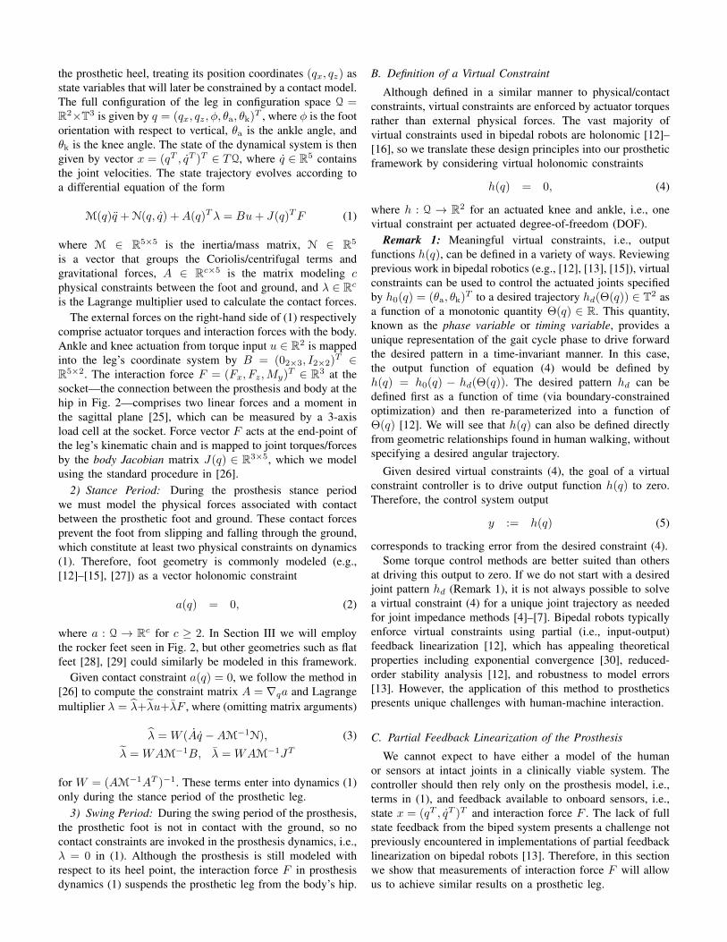
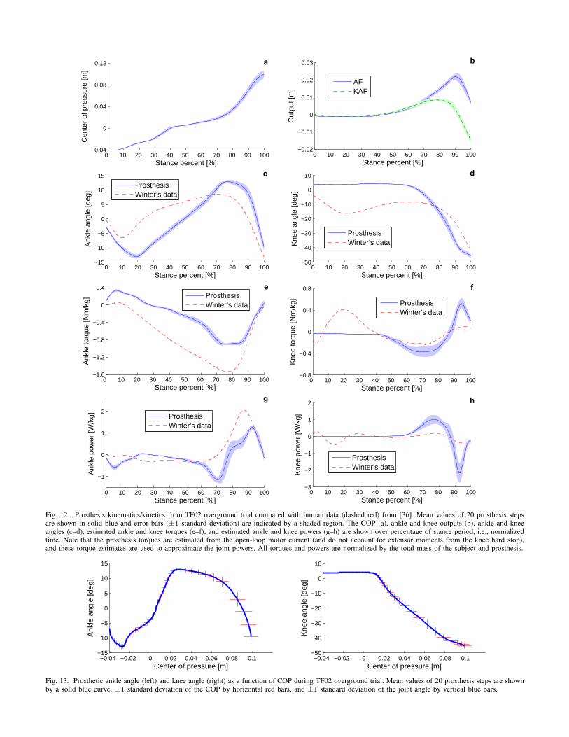
Focusing on the stance period of the prosthesis—when thevirtual constraint controller was employed—Fig. 12 shows themean data for 20 overground steps by TF02. We see in Fig. 12athat the COP moved monotonically from heel to toe, implyingthat it served as the phase variable of the virtual constraintsas intended. The outputs of the virtual constraints stayed in asmall neighborhood about zero (Fig. 12b), demonstrating thatthe clinically viable controller (9) reasonably approximatedthe theoretical controller (8) to enforce the virtual constraints.Our choice of effective shape as the virtual constraints resultedin the ankle and knee patterns progressing as a function ofthe COP as seen in Fig. 13. Note that the joint patterns lookdifferent over the phase variable than over time (Fig. 12c–d)because the COP did not increase linearly with respect to time,i.e., the phase domain in which control law (9) operated wasa warped representation of the time domain [42].

We did not observe any meaningful differences between theoverground and treadmill conditions besides reduced variancein the treadmill data. The phase portraits of the three subjectsduring the treadmill condition (Fig. 14) suggest the existenceof a stable limit cycle. As predicted by our simulations,the controller maintained invariant effective shapes acrossthe three treadmill speeds (Fig. 15), resembling able-bodiedbehavior reported in [22]. The maximum speed reached bythe subject pool was 1.03 m/s (TF01), which is notably fastfor a transfemoral amputee. We see in Fig. 16 that this subjectachieved a natural vertical ground reaction force (GRF) profilewith the prosthesis, including an initial hump during early-stance loading and a final hump at late-stance pushoff. Thissecond hump, which is indicative of active propulsion, cannotbe achieved with most transfemoral prostheses [2].

Analysis of the prosthetic joint kinematics and kineticsreveals that the virtual constraint controller produced joint

0 10 20 30 40 50 60 70 80 90 100−0.04

0

0.04

0.08

0.12

Stance percent [%]

Cen

ter

of p

ress

ure

[m]

a

0 10 20 30 40 50 60 70 80 90 100−0.02

−0.01

0

0.01

0.02

0.03

Stance percent [%]

Out

put [

m]

AFKAF

b

0 10 20 30 40 50 60 70 80 90 100−15

−10

−5

0

5

10

15

Stance percent [%]

Ank

le a

ngle

[deg

]

ProsthesisWinter’s data

c

0 10 20 30 40 50 60 70 80 90 100−50

−40

−30

−20

−10

0

10

Stance percent [%]

Kne

e an

gle

[deg

]

ProsthesisWinter’s data

d

0 10 20 30 40 50 60 70 80 90 100−1.6

−1.2

−0.8

−0.4

0

0.4

Stance percent [%]

Ank

le to

rque

[Nm

/kg]

ProsthesisWinter’s data

e

0 10 20 30 40 50 60 70 80 90 100−0.8

−0.4

0

0.4

0.8

Stance percent [%]

Kne

e to

rque

[Nm

/kg]

ProsthesisWinter’s data

f

0 10 20 30 40 50 60 70 80 90 100

−1

0

1

2

Stance percent [%]

Ank

le p

ower

[W/k

g] ProsthesisWinter’s data

g

0 10 20 30 40 50 60 70 80 90 100−3

−2

−1

0

1

2

Stance percent [%]

Kne

e po

wer

[W/k

g]

ProsthesisWinter’s data

h

Fig. 12. Prosthesis kinematics/kinetics from TF02 overground trial compared with human data (dashed red) from [36]. Mean values of 20 prosthesis stepsare shown in solid blue and error bars (±1 standard deviation) are indicated by a shaded region. The COP (a), ankle and knee outputs (b), ankle and kneeangles (c–d), estimated ankle and knee torques (e–f), and estimated ankle and knee powers (g–h) are shown over percentage of stance period, i.e., normalizedtime. Note that the prosthesis torques are estimated from the open-loop motor current (and do not account for extensor moments from the knee hard stop),and these torque estimates are used to approximate the joint powers. All torques and powers are normalized by the total mass of the subject and prosthesis.

−0.04 −0.02 0 0.02 0.04 0.06 0.08 0.1−15

−10

−5

0

5

10

15

Center of pressure [m]

Ank

le a

ngle

[deg

]

−0.04 −0.02 0 0.02 0.04 0.06 0.08 0.1−50

−40

−30

−20

−10

0

10

Center of pressure [m]

Kne

e an

gle

[deg

]

Fig. 13. Prosthetic ankle angle (left) and knee angle (right) as a function of COP during TF02 overground trial. Mean values of 20 prosthesis steps are shownby a solid blue curve, ±1 standard deviation of the COP by horizontal red bars, and ±1 standard deviation of the joint angle by vertical blue bars.

−60 −40 −20 0 20−400

−200

0

200

400

Angle [deg]

Vel

ocity

[deg

/s]

Ankle (TF01)Knee (TF01)Ankle (AB)Knee (AB)

−60 −40 −20 0 20−400

−200

0

200

400

Angle [deg]

Vel

ocity

[deg

/s]

Ankle (TF02)Knee (TF02)Ankle (AB)Knee (AB)

−60 −40 −20 0 20−400

−200

0

200

400

Angle [deg]

Vel

ocity

[deg

/s]

Ankle (TF03)Knee (TF03)Ankle (AB)Knee (AB)

Fig. 14. Prosthetic phase portrait (joint angles vs. velocities) over 20 gait cycles for self-selected treadmill condition of subjects TF01 (left), TF02 (center),and TF03 (right), compared to mean able-bodied (AB) data from [36]. Note that the able-bodied data does not necessarily match each amputee subject’sweight or speed. The prosthetic joint trajectories appear to converge to a periodic orbit—known as a limit cycle—as the subject approached steady state. Wesuspect that TF03, whose weight was at the upper bound of our inclusion criteria, experienced greater variability because of more frequent actuator saturation.

behavior that was close to normal. The ankle angle trajectoryin Fig. 12c follows the same trends as Winter’s able-bodieddata [36], starting with a period of controlled plantarflexion asthe foot progressed from heel-strike to foot-flat. Subsequentlyas the leg rotated over the foot, the ankle dorsiflexed untila peak of about 13 degrees was reached at about 70% ofstance. The movement then reversed as the ankle activelyplantarflexed, which we see in the torque estimated from themotor current in Fig. 12e. At this point the controller provideda powered push-off (Fig. 12g), thus contributing activelyto the energetics of walking. The ankle did not reach thephysiologically appropriate peak torque because its actuatorsaturated at 80 N·m (see Fig. 12e). Note that the differencesbetween the experimental torques here and the simulatedtorques in Section IV can be attributed to inaccuracies in thecontact model (Section IV-E) and the downhill slope conditionused in the simulations, requiring different values for shapeparameters Xs, Xt, Zs, and Zt in the prosthesis controller.

Although the prosthesis controller provided knee flexionduring early stance in the simulations of Section IV, we didnot observe this natural behavior in our experiments (Fig. 12d).All subjects intentionally locked the knee while loading bodyweight on the leg, which most prosthesis users do to ensurethe knee does not buckle [2]. The knee torque plot of Fig. 12fdoes not show a subsequent extensor moment as in Winter’sdata, but examination of the prosthetic knee angle shows thatthe joint was against the hard stop at 4 degrees, which providedan unmeasured extensor moment. Late-stance knee flexion wasclose to natural and in synergy with ankle push-off, allowingthe transfer of positive propulsive energy to the user. In fact,the total mechanical work done by the prosthetic leg duringstance (normalized by the mass of the subject and prosthesis)was positive for two of the three subjects: 0.0817 J/kg forTF16, 0.0436 J/kg for TF01, and −0.0541 J/kg for TF02,compared to 0.109 J/kg in Winter’s able-bodied data. Wesuspect that the prosthesis did negative net work for TF02because of his use of the handrails (which may have dissipatedenergy) and less ankle pushoff (at his request).

VI. DISCUSSION

Our control strategy produced close-to-normal walkingpatterns for transfemoral amputee subjects using normalized

−0.05 0 0.05 0.1

−0.1

−0.08

−0.06

−0.04

x−axis [m]

z−ax

is [m

]

AF able−bodiedKAF able−bodiedAF @ 0.76 m/sKAF @ 0.76 m/sAF @ 0.89 m/sKAF @ 0.89 m/sAF @ 1.03 m/sKAF @ 1.03 m/s

Fig. 15. Prosthetic effective shapes at variable cadences from TF01 treadmilltrial (averaged across 20 steps for each cadence), compared with able-bodiedshapes from overground walking at normal cadence reported in [22]. End ofstance is indicated by a circle. The prosthetic effective shapes appear to beinvariant across cadences as observed in able-bodied studies [22]. A ‘hook’occurs during double support in both the prosthetic and able-bodied shapes.

0 10 20 30 40 50 60 70 80 90 100Stance percent [%]

Ver

tical

GR

F

ProsthesisWinter’s data

Fig. 16. Vertical GRF measured from instrumented prosthetic foot duringTF01 fast treadmill trial, compared with Winter’s data measured from a forceplate during overground walking [36]. The profiles are scaled vertically tocompensate for differences in task and measurement technique. Mean valuesof 20 prosthesis steps are shown in solid blue and error bars (±1 standarddeviation) are indicated by a shaded region. Note the double-hump in the forceprofile—one during early-stance loading and one during late-stance pushoff.

effective shape parameters from the literature. The simulationsof Section IV verified the robustness of the virtual constraintapproach to experimental conditions, and by approximating thedesired partial feedback linearization we appeared to achievestability in our experiments. We observed convergence to aperiodic orbit—known as a hybrid limit cycle—in the phaseportraits of Fig. 14, suggesting that the controller enabled asteady-state gait pattern for the amputee subjects. Given that

the outputs remained in a small neighborhood about zero,control law (9) created approximate hybrid zero dynamicsthat were stabilized by the human-in-the-loop, demonstratingsuccessful human-machine interaction in the context of virtualconstraints. In fact, most subjects did not use the handrails tomaintain gait stability with the experimental prosthesis.

A. Strengths of the ApproachThis work shows that knee and ankle control during stance

can be coordinated by one simple objective: maintaininga constant curvature in the effective shapes. Coordinationand synchrony between leg joints (e.g., through biarticularmuscles) are important to energetic efficiency [43] androbustness [19], but coordinated control is uncommon incurrent multi-joint prostheses. Control law (9) coordinatedknee control with the ankle joint to enforce the KAF effectiveshape, which explicitly depends on the ankle angle (AppendixB). Knee and ankle patterns were also synchronized by theirdependence on the same phase variable (Remark 4). Onesubject claimed to notice the two joints working in unison.

By relying on meaningful parameters for clinicians, theproposed control approach could potentially improve theclinical viability of powered prosthetic legs. The effective radiiRs = Rt and centers Xs = Xt are defined by simple fractionsof the user’s height [22], preventing the need for hand-tuning. We also demonstrated that the five non-anatomicalparameters Kps, Kpt, Kds, Kdt, and Kdts can be normalizedby body mass as a starting point for walking on the prosthesis.These are the only hand-tuned parameters for stance, whereasexisting approaches have more hand-tuned parameters for thisperiod (e.g., 18 for impedance control with three stance phases[5] or more with Hill-type muscle models [7]). By using onecontrol model during stance, we also eliminated two controlswitches and their hand-tuned rules compared to [5], [7].However, future randomized clinical studies are needed tocompare the performance of these different control methods.

The invariance of the effective shape across conditionssuch as walking speed [22], heel height [23], shoe curvature[24], and body weight [21] suggests that this choice ofvirtual constraint could make prosthetic legs more adaptablethan conventional prostheses, which cause discomfort andinstability as these conditions vary. Our treadmill experimentsverified the simulations showing that our control systemadjusts to variable walking speeds by enforcing the effectiveshapes. Although the AF effective shape can also be achievedwith the passive Shape&Roll foot [38], this below-knee devicecannot regulate the KAF effective shape. Moreover, thispassive prosthesis can only be tuned to one task at a time,whereas humans employ effective shapes unique to differenttasks. For example, the shape curvature changes substantiallybetween walking and stationary standing [34], and upstairsclimbing requires a completely different geometry [35] withpositive mechanical work. For this purpose virtual constraintscan be defined with non-constant curvature in (12), wherethe effective shapes associated with stairs may be the mostdifficult to model [35]. Our control method could implementvirtual constraints for any effective shape, by which a poweredprosthetic leg could perform a wide variety of tasks.

We did not explicitly design an ankle push-off period intothe control strategy, but enforcing the effective shape as avirtual constraint provided a period of power generation asthe COP approached the toe. A positive feedback loop arosewhen COP movement caused a plantarflexive ankle torque,which in turn caused the COP to move further forward. Duringearly stance this positive feedback loop was counteracted bya negative feedback loop involving the moment arm fromshear forces. Because forces are transferred down the leg fromthe socket, subjects were able to influence these feedbackloops and consequently their progression through the step. Webelieve this allowed subjects to walk at their preferred speedoverground and accommodate variable speeds on the treadmill.Positive force feedback has been observed during late stancein able-bodied gait [44], but this biomimetic behavior wasonly previously reproduced in a prosthesis using muscle reflexmodels [7]. Although we did not tune our control system tomaximize positive work, the energy production we observedwas likely associated with this positive feedback. This featurein a prosthetic leg might prevent compensatory work at the hip[3] and allow lower-limb amputees to expend normal levelsof energy when walking [2]. However, this positive feedbackloop should be disabled during stationary standing, as COPdrift towards the toe could cause unintended ankle pushoff.

B. Limitations of the Study

The use of approximate feedback linearization resulted ina few discrepancies during mid-late stance. Excessive ankledorsiflexion in Fig. 12c was associated with tracking errorfrom the desired effective shapes, which grew during mid-latestance in both the simulations (Fig. 5) and experiments (Fig.12b). We suspect that the approximate controller could notcompensate for stronger nonlinearities during this period ofgait, especially in the presence of ankle actuator saturation(Fig. 12e) and small PD gains. We employed small gainsfor the safety of our subjects, who may have helped virtualconstraint enforcement through the socket interaction forces,which enter into the output dynamics (6). Future workcould compensate for nonlinearities by using larger PD gainsduring mid-late stance (via phase-based gain scheduling),simultaneous linear control methods [45], or the exactfeedback linearization of Section II-C. Performance could befurther improved with series elastic actuation [46], which canprovide closed-loop torque control and larger peak torques.

The prosthetic foot used in these experiments violatedour model’s point-contact assumption (the COP was notdependent on configuration alone as assumed in Section II-E),implying that the effective shape was not truly holonomic.Our experiments successfully employed these nonholonomicconstraints, e.g., output functions of the form h(q, q), in theapproximate control law (9), demonstrating some robustnessto unmodeled dynamics. The exact control law (8) couldalso be reformulated for nonholonomic constraints as in[29], resulting in lower-order output dynamics and higher-order zero dynamics. However, the vast majority of bipedalrobots [12]–[16] use holonomic virtual constraints for lower-dimensional stability analysis (Remark 2), motivating our

holonomic treatment in this paper. We employed the effectiveshape as a starting point for this research, but future workcould find better choices of virtual constraints for use in thegeneral control framework of Section II.

For example, we could model non-constant curvature intothe effective shape during the double-support period to bettermimic able-bodied gait (Fig. 15, [21]). For simplicity wecontinued using the constant-curvature virtual constraints (12)as the prosthesis entered double support with the intactleg. We see in Fig. 15 that the approximate controller (9)provided compliance during this period to resemble able-bodied effective shapes, but the stance-to-swing transition(when the most KAF tracking error occurred) was a source ofcriticism from the subjects. A more general model of effectiveshape with non-constant curvature in (11) could potentiallybe used in the future to explicitly enforce the appropriateshape during double support. Replacing the joint impedancecontroller of the swing period with a minimum-jerk controlstrategy [47] may also help the stance-to-swing transition.Alternatively, a definition of effective shape for the swingperiod would allow the use of virtual constraints, resultingin a unified swing period to further reduce the number ofcontrol switches and hand-tuned parameters. This developmentmay require a new phase variable that is measurable fromthe prosthesis during swing (see initial work in [48]). Onlyafter these promising directions are investigated will the virtualconstraint approach be mature enough for clinical comparisonwith state-of-the-art impedance control methods [4]–[6].

VII. CONCLUSION

These simulations and experiments demonstrate that thetheory of virtual constraints could provide a clinically viablesolution for unified control of powered prosthetic legs. Inparticular, our stance control strategy produced biomimetic,robust, and coordinated ankle-knee movement on a prostheticleg used by amputee subjects. The controller was able tooperate at variable cadences without changes to controlparameters due to the invariance of the effective shape, whichalso holds over shoe geometries and body weights [21].

Our simulations suggest that the proposed control approachcan also accommodate inclines, motivating future experimentswith ramps and stairs. More demanding tasks like runningmay require the exact feedback linearization in SectionII-C to prevent output tracking error, necessitating systemidentification of the intrinsic dynamics of the prosthetic leg.Our control approach could also be integrated with a neuralinterface (e.g., using electromyography from residual muscles[49]) to allow the user to subconsciously switch betweenvirtual constraints when anticipating a task change.

The significance of effective shape begs the question as towhether human locomotion might employ a phase variable[42], [48]. Phase-based virtual constraints could also beapplied to powered exoskeletons (e.g., [11]), motivating futureinvestigation of hybrid zero dynamics for wearable robots.With further development the proposed control concepts havethe potential to improve mobility and quality of life forindividuals after amputation, stroke, or spinal cord injury.

Acknowledgments

The authors thank Andrew Hansen for discussions on hisstudies, the CBM electronics team for the load cell electronics,Nicholas Fey and Annie Simon for support with the Vanderbiltleg, and Suzanne Finucane, PTA and Robert Lipschutz, CP forclinical support during the amputee subject experiments.

APPENDIX

A. Contact Constraints

Because a rolling contact point has zero velocity at anyinstant [25], we simplify model-based calculations by treatingthis contact point (the COP) as stationary and modeling thekinematic chain with respect to an inertial frame defined atthe COP. This assumption physically corresponds to rollingon an ideal treadmill, which can approximate the curvature ofhuman foot compliance, i.e., the relative motion between theCOP and heel, in a similar manner to rolling overground. Wemodel the foot as an arc of radius Rf going through the heel(qx, qz) and the COP. The vector from the COP to the centerof rotation Pf is defined normal to the ground and constrainedby ||Pf−COP || = Rf , yielding equation aroll1 (q) = 0. We alsoconstrain the foot orientation φ so the heel is perpendicular tothe foot arc (Fig. 2), yielding equation aroll2 (q) = 0.

B. Virtual Constraints

The AF effective shape is the distance constraint (11)between the COP and the center of rotation Ps in the shank-based reference frame of Fig. 3 (left). In model coordinates qdefined with respect to the COP, Ps is given by the function

PCOPs (q) = (qx, qz)T +`f(− sin(φ), cos(φ))T +S(φ+θa)Ps,

where S is the standard 2×2 rotation matrix parameterized byangle φ+θa. Similarly, the KAF effective shape is the distanceconstraint (11) between the COP and the center of rotation Pt

in a thigh-based reference frame (Fig. 3, right). The point Pt

is given in model coordinates by the function

PCOPt (q) = (qx, qz)T + `f(− sin(φ), cos(φ))T + S(ρ)Pt,

where rotation matrix S is parameterized by angle

ρ = φ+ arctan(`s sin(θa) + `t sin(θa + θk)

`s cos(θa) + `t cos(θa + θk)).

Finally, these functions define the virtual constraints by (12).

C. Instrumented Foot

We designed the instrumented prosthetic foot in Fig. 10 tomeasure the COP for our controller as initially reported in[20]. Two aluminum plates were mounted around two 6-axisload cells (model: Mini45, ATI Industrial Automation, Apex,NC) with one cell towards the heel and the other towards thetoe. This configuration distributed loads encountered duringwalking to prevent sensor saturation and bending moments.The top plate was mounted to the bottom of the leg’s anklejoint, and the bottom plate was mounted to a carbon fiberprosthetic foot plate; the configured leg is shown in Fig. 9

(left). The assembled foot adapter (load cells and aluminumplates) added 0.79 kg to the weight of the foot plate.

The two aluminum plates of the foot adapter weremechanically coupled only through the load cells, by whichwe measured the loads transferred between the leg and ground.We used a free-body diagram to solve for the COP:

qx =My1 +My2 + bv(Fx1 + Fx2) + bh(Fz2 − Fz1)

Fz1 + Fz2,

where Fxi and Fzi are the horizontal and vertical loads,respectively, at the heel (i = 1) or toe (i = 2), bv = 5.08 cm isthe vertical distance between the bottom of the foot plate andthe reference frame of each load cell, and bh = 7 cm is thehorizontal distance between the ankle joint and the referenceframe of each load cell (Fig. 10). This calculation requires onlythree of the six strain gauges in each ATI load cell, which waschosen for compactness, weight, and load ratings. All six straingauges could be used to measure the 3D GRF vector, allowingselective saturation of control torques to keep the GRF withinthe friction cone and thus prevent the foot from slipping.

We did not have an inertial measurement unit to measureheel rise and foot rotation, so we approximated these variablesbased on the rocker-foot contact model in Appendix A.

REFERENCES

[1] W. Miller, A. Deathe, M. Speechley, and J. Koval, “The influence offalling, fear of falling, and balance confidence on prosthetic mobility andsocial activity among individuals with a lower extremity amputation,”Arch. Phys. Med. Rehab., vol. 82, no. 9, pp. 1238–1244, 2001.

[2] D. G. Smith, J. W. Michael, and J. H. Bowker, Eds., Atlasof Amputations and Limb Deficiencies: Surgical, Prosthetic, andRehabilitation Principles. Rosemont, IL: American Academy ofOrthopaedic Surgeons, 2004.

[3] J. Johansson, D. Sherrill, P. Riley, P. Bonato, and H. Herr, “A clinicalcomparison of variable-damping and mechanically passive prostheticknee devices,” Amer. J. Phys. Med. Rehab., vol. 84, no. 8, pp. 563–575, 2005.

[4] F. Sup, A. Bohara, and M. Goldfarb, “Design and control of a poweredtransfemoral prosthesis,” Int. J. Robot. Res., vol. 27, no. 2, pp. 263–273,2008.

[5] F. Sup, H. Varol, and M. Goldfarb, “Upslope walking with a poweredknee and ankle prosthesis: Initial results with an amputee subject,” IEEETrans. Neural Sys. Rehab. Eng., vol. 19, no. 1, pp. 71–78, 2011.

[6] A. Simon, N. Fey, S. Finucane, R. Lipschutz, and L. Hargrove,“Strategies to reduce the configuration time for a powered knee andankle prosthesis across multiple ambulation modes,” in IEEE Int. Conf.Rehab. Robot., Seattle, WA, 2013.

[7] M. Eilenberg, H. Geyer, and H. Herr, “Control of a powered ankle–footprosthesis based on a neuromuscular model,” IEEE Trans. Neural Sys.Rehab. Eng., vol. 18, no. 2, pp. 164–173, 2010.

[8] J. L. Stein and W. C. Flowers, “Stance phase control of above-kneeprostheses: Knee control versus SACH foot design,” J. Biomech., vol. 20,no. 1, pp. 19–28, 1987.

[9] M. A. Holgate, T. G. Sugar, and A. W. Bohler, “A novel controlalgorithm for wearable robotics using phase plane invariants,” in IEEEInt. Conf. Robot. Automat., Kobe, Japan, 2009, pp. 3845–3850.

[10] A. W. Boehler, K. W. Hollander, T. G. Sugar, and D. Shin, “Design,implementation and test results of a robust control method for apowered ankle foot orthosis (AFO),” in IEEE Int. Conf. Robot. Automat.,Pasadena, CA, 2008, pp. 2025–2030.

[11] K. A. Shorter, E. T. Hsiao-Wecksler, G. F. Kogler, E. Loth, and W. K.Durfee, “A portable powered ankle-foot-orthosis for rehabilitation,” J.Rehab. Res. Dev., vol. 48, no. 4, pp. 459–472, 2011.

[12] E. R. Westervelt, J. W. Grizzle, C. Chevallereau, J. H. Choi, andB. Morris, Feedback Control of Dynamic Bipedal Robot Locomotion.New York, NY: CRC Press, 2007.

[13] K. Sreenath, H. W. Park, I. Poulakakis, and J. W. Grizzle, “A complianthybrid zero dynamics controller for stable, efficient and fast bipedalwalking on MABEL,” Int. J. Robot. Res., vol. 30, no. 9, pp. 1170–1193,2011.

[14] S. Kolathaya and A. D. Ames, “Achieving bipedal locomotion onrough terrain through human-inspired control,” in IEEE Int. Sym. SafetySecurity Rescue Robot., College Station, TX, 2012.

[15] A. Martin, D. Post, and J. Schmiedeler, “Design and experimentalimplementation of a hybrid zero dynamics controller for planar bipedswith curved feet,” Int. J. Robot. Res., vol. 33, no. 7, pp. 988–1005, 2014.

[16] A. Ramezani, J. W. Hurst, K. A. Hamed, and J. W. Grizzle, “Performanceanalysis and feedback control of ATRIAS, a 3D bipedal robot,” ASMEJ. Dyn. Sys. Meas. Control, vol. 136, no. 2, p. 021012, 2013.

[17] B. Espiau, “Sensor-based estimation of human motion for controlsynchronization,” in IEEE RO-MAN, Toyama, Japan, 2009.

[18] R. D. Gregg and J. W. Sensinger, “Towards biomimetic virtual constraintcontrol of a powered prosthetic leg,” IEEE Trans. Control Sys. Tech.,vol. 22, no. 1, pp. 246–254, 2014.

[19] ——, “Biomimetic virtual constraint control of a transfemoral poweredprosthetic leg,” in Amer. Control Conf., Washington, DC, 2013, pp.5702–5708.

[20] R. D. Gregg, T. Lenzi, N. P. Fey, L. J. Hargrove, and J. W. Sensinger,“Experimental effective shape control of a powered transfemoralprosthesis,” in IEEE Int. Conf. Rehab. Robot., Seattle, WA, 2013.

[21] A. Hansen and D. Childress, “Investigations of roll-over shape:Implications for design, alignment, and evaluation of ankle-footprostheses and orthoses,” Dis. Rehab., vol. 32, no. 26, pp. 2201–2209,2010.

[22] A. Hansen, D. Childress, and E. Knox, “Roll-over shapes of humanlocomotor systems: Effects of walking speed,” Clin. Biomech., vol. 19,no. 4, pp. 407–414, 2004.

[23] A. Hansen and D. Childress, “Effects of shoe heel height on biologicrollover characteristics during walking,” J. Rehab. Res. Dev., vol. 41,no. 4, pp. 547–554, 2004.

[24] C. Wang and A. Hansen, “Response of able-bodied persons to changesin shoe rocker radius during walking: Changes in ankle kinematics tomaintain a consistent roll-over shape,” J. Biomech., vol. 43, no. 12, pp.2288–2293, 2010.

[25] R. C. Hibbeler, Engineering Mechanics: Dynamics, 13rd ed. UpperSaddle River, NJ: Prentice Hall, 2012.

[26] R. M. Murray, Z. Li, and S. S. Sastry, A Mathematical Introduction toRobotic Manipulation. Boca Raton, FL: CRC Press, 1994.

[27] A. Martin and J. Schmiedeler, “Predicting human walking gaits with asimple planar model,” J. Biomech., vol. 47, no. 6, pp. 1416–1421, 2014.

[28] R. D. Gregg, Y. Y. Dhaher, A. Degani, and K. M. Lynch, “On themechanics of functional asymmetry in bipedal walking,” IEEE Trans.Biomed. Eng., vol. 59, no. 5, pp. 1310–1318, 2012.

[29] R. D. Gregg and L. Righetti, “Controlled reduction with unactuatedcyclic variables: Application to 3D bipedal walking with passive yawrotation,” IEEE Trans. Automat. Contr., vol. 58, no. 10, pp. 2679–2685,2013.

[30] A. Isidori, Nonlinear Control Systems: An Introduction, 3rd ed. Berlin,Germany: Springer-Verlag, 1995.

[31] A. Goswami, B. Thuilot, and B. Espiau, “A study of the passive gait ofa compass-like biped robot: Symmetry and chaos,” Int. J. Robot. Res.,vol. 17, no. 12, pp. 1282–1301, 1998.

[32] A. D. Ames, K. Galloway, J. W. Grizzle, and K. Sreenath, “Rapidlyexponentially stabilizing control Lyapunov functions and hybrid zerodynamics,” IEEE Trans. Automat. Contr., vol. 59, no. 4, pp. 876–891,2014.

[33] A. Hansen, D. Childress, and E. Knox, “Prosthetic foot roll-over shapeswith implications for alignment of trans-tibial prostheses,” Prosth. Orth.Int., vol. 24, no. 3, pp. 205–215, 2000.

[34] A. Hansen and C. Wang, “Effective rocker shapes used by able-bodiedpersons for walking and fore-aft swaying: Implications for design ofankle-foot prostheses,” Gait Pos., vol. 32, no. 2, pp. 181–184, 2010.

[35] E. Sinitski, A. Hansen, and J. Wilken, “Biomechanics of the ankle-footsystem during stair ambulation: Implications for design of advancedankle-foot prostheses,” J. Biomech., vol. 45, no. 3, pp. 588–594, 2012.

[36] D. A. Winter, Biomechanics and Motor Control of Human Movement,2nd ed. New York, NY: Wiley, 2009.

[37] P. Adamczyk, S. Collins, and A. Kuo, “The advantages of a rolling footin human walking,” J. Exp. Bio., vol. 209, no. 20, p. 3953, 2006.

[38] M. Sam, D. Childress, A. Hansen, M. Meier, S. Lambla, E. Grahn,and J. Rolock, “The ‘Shape&Roll’ prosthetic foot: I. Design anddevelopment of appropriate technology for low-income countries,” Med.Confl. Surviv., vol. 20, no. 4, pp. 294–306, 2004.

[39] S. Mochon and T. A. McMahon, “Ballistic walking,” J. Biomech.,vol. 13, no. 1, pp. 49–57, 1980.

[40] A. Minetti, C. Moia, G. Roi, D. Susta, and G. Ferretti, “Energy cost ofwalking and running at extreme uphill and downhill slopes,” J. AppliedPhys., vol. 93, no. 3, pp. 1039–1046, 2002.

[41] P. De Leva, “Adjustments to Zatsiorsky-Seluyanov’s segment inertiaparameters,” J. Biomech., vol. 29, no. 9, pp. 1223–1230, 1996.

[42] R. D. Gregg, E. J. Rouse, L. J. Hargrove, and J. W. Sensinger, “Evidencefor a time-invariant phase variable in human ankle control,” PLoS ONE,vol. 9, no. 2, p. e89163, 2014, doi: 10.1371/journal.pone.0089163.

[43] A. Pedotti, “A study of motor coordination and neuromuscular activitiesin human locomotion,” Bio. Cybernetics, vol. 26, no. 1, pp. 53–62, 1977.

[44] V. Dietz and J. Duysens, “Significance of load receptor input duringlocomotion: A review,” Gait Pos., vol. 11, no. 2, pp. 102–110, 2000.

[45] A. Nanjangud and R. D. Gregg, “Simultaneous control of an ankle-footprosthesis model using a virtual constraint,” in ASME Dynamic SystemsControl Conf., San Antonio, TX, 2014.

[46] N. Paine, S. Oh, and L. Sentis, “Design and control considerationsfor high-performance series elastic actuators,” IEEE/ASME Trans.Mechatron., vol. 19, no. 3, pp. 1080–1091, 2014.

[47] T. Lenzi, L. J. Hargrove, and J. W. Sensinger, “A novel controlframework allowing physiological walking speed adaptation in poweredtransfemoral prostheses,” IEEE Robot. Automat. Mag., 2014, in press.

[48] D. J. Villarreal and R. D. Gregg, “A survey of phase variable candidatesof human locomotion,” in IEEE Int. Conf. Eng. Med. Biol. Soc., Chicago,IL, 2014.

[49] L. Hargrove, A. Simon, R. Lipschutz, S. Finucane, and T. Kuiken, “Real-time myoelectric control of knee and ankle motions for transfemoralamputees,” J. Amer. Med. Assoc., vol. 305, no. 15, pp. 1542–1544, 2011.

Robert D. Gregg (S’08-M’10) received the B.S.degree (2006) in electrical engineering and computersciences from the University of California, Berkeleyand the M.S. (2007) and Ph.D. (2010) degreesin electrical and computer engineering from theUniversity of Illinois at Urbana-Champaign.

He joined the Departments of Bioengineering andMechanical Engineering at the University of Texasat Dallas (UTD) as an Assistant Professor in 2013.Prior to joining UTD, he was a Research Scientistat the Rehabilitation Institute of Chicago and a

Postdoctoral Fellow at Northwestern University. His research is in the controlof bipedal locomotion with applications to autonomous and wearable robots.

Prof. Gregg is a recipient of the NIH Director’s New Innovator Award andthe Burroughs Wellcome Fund’s Career Award at the Scientific Interface. Healso received the 2011 CLAWAR Best Technical Paper Award, the 2009 O.Hugo Schuck Award of the IFAC American Automatic Control Council, andthe Best Student Paper Award of the 2008 American Control Conference.

Tommaso Lenzi (S’11-M’13) received theM.Sc. degree in biomedical engineering from theUniversity of Pisa, Pisa, Italy, in 2008, and thePh.D. degree in biorobotics, from Scuola SuperioreSant’Anna, Pisa, Italy, in 2012. He is currentlya Postdoctoral Fellow with the Center for BionicMedicine, Rehabilitation Institute of Chicago,and the Department of Physical Medicine andRehabilitation, Northwestern University, Chicago,IL, USA. From August 2011 to February 2012,he was Visiting Research Scientist with the

Department of Mechanical Engineering, University of Delaware, Newark,DE, USA. He has co-authored 16 ISI journal papers and 29 peer-reviewconference proceedings papers. His main research interests include robotics,mechatronics, and rehabilitation medicine, with a major emphasis on designand control of wearable robots for human assistance and rehabilitation.

Levi J. Hargrove (S’05-M’08) received hisB.Sc. and M.Sc. and PhD degrees in electricalengineering from the University of New Brunswick(UNB), Fredericton, NB, Canada, in 2003 2005,and 2007 respectively. He joined the Center forBionic Medicine at the Rehabilitation Institute ofChicago in 2008. His research interests includepattern recognition, biological signal processing,and myoelectric control of powered prostheses.Dr. Hargrove is a member of the Association ofProfessional Engineers and Geoscientists of New

Brunswick. He is also an Assistant Professor in the Department ofPhysical Medicine and Rehabilitation (PM&R) and Biomedical Engineering,Northwestern University, Evanston, IL, USA.

Jonathon W. Sensinger (M’09) received the B.S.degree in bioengineering from the University ofIllinois, Chicago, IL, USA, in 2002, and the Ph.D.degree in biomedical engineering from NorthwesternUniversity, Chicago, IL, USA, in 2007.

He is currently the Associate Director ofthe Institute of Biomedical Engineering and anAssociate Professor of Electrical and ComputerEngineering at the University of New Brunswick,Fredericton, NB, Canada. His research interestsinclude body-powered and robotic prosthesis design

and control, with interest in developing-world applications. He focuses onclinically relevant, low cost/weight systems. In addition, he performs researchin human-machine interfaces using haptics and computational motor controlapproaches with a goal to improve the control filtering and sensory feedbackoptions available to persons with an amputation.