1

COMPARING THE INCIDENCE OF TAXES AND SOCIAL SPENDING IN BRAZIL AND THE UNITED STATESSean Higgins,a Nora Lustig,b Whitney Rublea and Timothy Smeedingc

CEQ Working Paper No 16

NOVEMBER 2013

Revised OCTOBER 2014a Ph.D. Student, Department of Economics, Tulane Universityb Samuel Z. Stone Professor of Latin American Economics, Tulane

University; Nonresident Fellow, Center for Global Development and Inter-American Dialoguec Director, Institute for Research on Poverty; Arts and Sciences Distinguished Professor of Public Affairs and Economics, University of Wisconsin at Madison

ABSTRACT

We perform the first comprehensive fiscal incidence analyses in Brazil and the US, including direct cash and food transfers, targeted housing and heating subsidies, public spending on education and health, and personal income, payroll, corporate income, property, and expenditure taxes. The countries share a number of similarities that make the comparison interesting, including high levels of inequality given their level of development, high inequality of opportunity, a large and racially diverse population, and similar size of government. The US achieves higher redistribution through direct taxes and transfers, primarily due to underutilization of the personal income tax in Brazil and the fact that Brazil’s highly progressive cash and food transfer programs are small while its larger transfer programs are less progressive. However, when health and non-tertiary education spending are added to income using the government cost approach, the two countries achieve similar levels of redistribution.

JEL: D31, H22, I38

Keywords: inequality, fiscal policy, taxation, social spending

1

1 INTRODUCTION

Both Brazil and the United States have been persistently unequal given their levels of development. A quarter century ago, Brazil had one of the highest levels of inequality in the world, while the US had one of the highest levels of inequality among developed countries.1 These high levels of inequality have persisted: although Brazil’s level of inequality has recently fallen (Lustig et al., 2013b), it is still among the twenty most unequal countries in the world (Alvaredo and Gasparini, forthcoming); inequality in the US has been rising (Kenworthy and Smeeding, 2014) and it is now the third most unequal OECD country behind Chile and Mexico.2 Furthermore, when the US was at a similar level of development as Brazil is today, it had similar levels of inequality (Plotnick et al., 1998).3 In both countries, one key determinant of income inequality is the unequal distribution of human capital associated with high rates of school incompletion and, to some extent, race (Card and Krueger, 1992, Goldin and Katz, 2008, Ñopo, 2012). Both countries also face high inequality of opportunity (Bourguignon et al., 2007, Brunori et al., 2013), low levels of intergenerational mobility (Jäntti et al., 2006, Corak, 2013), and a similar profile with respect to income polarization (Ferreira et al., 2013, figure F5.1C).

In this paper, we investigate an important aspect of the two countries’ high level of inequality: the amount of redistribution and inequality reduction they achieve through social spending and taxes. Given the countries’ high inequality relative to their levels of development, as well as other similarities (large geographic area, large and diverse population, and similar size of government4), policymakers in both countries might benefit from a comparison of the redistributive effects of taxes and social spending in the two countries. We perform comprehensive fiscal

1 In 1989, Brazil’s Gini coefficient made it the second most unequal country in the world, second only to Sierra Leone (Ferreira et al., 2008); in 1985, the United States was the second most unequal OECD country (of countries that were OECD members in 1985), second only to Turkey (OECD, 2011a).2 The US is third most unequal using the 90/10 measure and fourth most unequal, also behind Turkey, using the Gini (OECD, 2014). The finding that income inequality in the US is higher than in other developed countries is not an artifact of using “snapshot” cross-section data to measure inequality: when the time horizon is extended to several years, income inequality in the United States is still higher than in other advanced countries (Aaberge et al., 2002).3 Plotnick et al. (1998) estimate that the Gini coefficient of monetary gross income in the United States in 1940—when GDP per capita was around $9,500 in 2009 dollars using GDP estimates from Bureau of Economic Analysis (2013) and population estimates from U.S. Census Bureau (2000)—was around 0.55, similar to the level observed in Brazil today. In Brazil, GDP per capita in 2012 was $11,720 (World Bank, 2013). Also see Atkinson and Morelli (2012) which contains a longer time series of Gini estimates in Brazil and the US.4 Combined primary spending by federal, state, and local governments is close to 40 percent of GDP in both countries. More specifically, Brazil’s consolidated primary spending (total spending minus interest payments) was 41.4 percent of GDP in 2009 (Ministério da Fazenda, 2010a), while it was 38.6 percent of GDP in the US in 2011 (International Monetary Fund, 2013, table 4a).

2

incidence analyses for both countries, including assessments of the progressivity of all major tax and transfer programs, to measure the impact of public spending and taxation on inequality in the two countries. Our analysis includes direct cash and food transfers, direct personal income, payroll, corporate income, and property taxes, indirect expenditure taxes, indirect subsidies for energy and housing, and spending on government-provided health and non-tertiary education. By including government spending on education and health, we are able to assess whether these components change our conclusions substantially, as was the case in Garfinkel et al.’s (2006, 2010) comparison between the United States and other OECD countries.

Our study of inequality in both the United States and Brazil makes several improvements over the existing literature. Existing studies usually omit indirect taxes and public spending on education and health (e.g., Immervoll et al. (2009) for Brazil and Kim and Lambert (2009) for the United States). For the US, the one study we are aware of that includes both indirect taxes and these in-kind benefits (Garfinkel et al., 2006, 2010) uses data from 2000. In the areas of allocating taxes and public spending on health and education, our study uses more robust methodologies than did earlier authors. For example, we use microsimulation results that take into account the fact that different states in the US have vastly different sales and property tax mixes—some much more regressive than others (Newman and O’Brien, 2011). For health and education spending, we use data on Medicare and Medicaid coverage to determine the distribution of health benefits, and use multiple household surveys to determine the distribution of education benefits given the lack of data on public vs. private school attendance in our main survey. In addition, we include imputed rent for owner-occupied housing, which is omitted from most studies on the US despite being an important component of income for the elderly (Bradbury, 2013).

In the case of Brazil, we build on the comprehensive incidence analysis undertaken by Higgins and Pereira (2014). Our main improvements—in addition to comparing results for Brazil to those of the US—are that here we use an improved methodology described in Lustig and Higgins (2013) when imputing public spending on education and health, include the corporate income tax, and use square root scale equivalized income rather than household per capita income. The use of equivalized rather than household per capita income avoids taking the extreme stance that there are no economies of scale within households, which would imply that fulfilling the needs of each additional household member

3

is just as costly as fulfilling the needs of the previous household member (see Buhmann et al., 1988).5

Another contribution of our paper is to compare the redistributive effects of the revenue collection and social spending systems in the two countries using a consistent and comprehensive framework. Direct comparisons between the two countries are rare; Bourguignon et al. (2008) decompose differences in the household income distributions in the two countries, but the only component of government spending and taxation they analyze is direct transfers. Multi-country studies that include both the US and Brazil similarly tend to overlook subsidies, expenditure taxes, and/or public spending on health and education.

Our comparison leads to a number of new insights. Before adding government spending on health and education to income, Brazil’s lower level of redistribution can be attributed to three main factors: Brazil’s direct taxes are both considerably smaller as a percent of GDP and considerably less progressive than those in the US; Brazil’s highly progressive direct transfer programs are small while its larger direct transfer programs are less progressive; and Brazil begins with a more unequal market income distribution (which limits redistributive capacity, as shown by Engel et al. (1999)). When government spending in health and education are included, however, the two countries reduce inequality by a similar amount.

The next section overviews the methodology used in the analysis including the methods used to allocate and estimate specific taxes and benefits, definitions of income concepts, and assumptions. It also describes our data and provides more detail about how we estimated taxes paid and benefits received for specific taxes and social spending components. Section 3 presents results for the two countries and discusses them in comparison. Section 4 concludes.

2 DATA, METHODOLOGY, AND INCOME CONCEPTS

Using the methodological framework proposed in Lustig and Higgins (2013) to ensure maximum comparability across countries in concept and estimate, we perform comprehensive fiscal incidence analyses to measure the effect of taxation and social spending on inequality in the two countries. The methodology consists of conventions for harmonizing the household survey microdata for maximum comparability, a set of strategies to allocate taxes and benefits to households

5 In Appendix A of the online supplement, we present inequality results across income concepts in Brazil and the United States using the two extremes of no economies of scale and complete economies of scale, which illustrate the robustness of our results to a variety of assumptions about economies of scale within households.

4

when these are not directly included as survey questions, definitions of a set of income concepts, and assumptions about the economic incidence of taxes and benefits. We summarize each of these aspects of the methodology in turn, then address limitations of our analysis. Our primary data sources are the 2011 Current Population Survey (CPS) for the US and the 2008-2009 Pesquisa de Orçamentos Familiares (POF) for Brazil; these are supplemented by the 2011 American Community Survey (ACS), 2011 American Housing Survey (AHS), and 2007 National Household Education Survey (NHES) in the US, and the 2008 Pesquisa Nacional por Amostra de Domicílios (PNAD) in Brazil.

i Harmonization

Following Lustig and Higgins (2013), we exclude “external” members of the household: boarders, live-in domestic servants, and their families (as well as their incomes) are dropped.6 Missing incomes due to item nonresponse are treated as zero, unless the household head’s primary income source is missing, in which case the household is dropped from the analysis. Households with zero gross income are also dropped, but households with zero market income and positive gross income (i.e., they receive all of their income from government transfers) are included. Households with zero gross income are very rare since this income concept includes imputed rent for owner occupied housing, government cash and food transfers, and (in the case of Brazil) the value of own production.

The complex sampling design of the surveys is accounted for by using the sampling weights included in each microdata set in all calculations. The standard errors in Table 3 also account for the stratified complex survey sampling. Household sampling weights are multiplied by the size of the household, so that our inequality estimates correspond to individual- rather than household-level inequality. We do not inflate totals for various income components in the survey to match those available from national accounts given fundamental differences between the two (Deaton, 2001); hence, to avoid overestimating the redistributive effect of health and education benefits (which are imputed based on spending from national accounts) we scale these benefits down to match survey magnitudes. Specifically, we ensure that the ratios of each component of health and non-tertiary education spending in national accounts to disposable income in national accounts equal the analogous ratios of these benefits to disposable income in our household surveys.

ii Allocation Methods

When a survey includes a specific question about the amount a household paid or received of a certain tax or transfer, the tax or transfer is directly identified. In 6 This is the convention followed by the Luxembourg Income Study (LIS), the Socioeconomic Database for Latin America (SEDLAC), and for most countries, the World Bank’s PovcalNet.

5

some cases, there is not a specific question for a particular transfer, but these are instead grouped into one question that also includes other sources of income. In this case, the transfer can sometimes be inferred based on whether the value the household reports in that income category matches a possible value of the transfer in question. When information available in the survey does not permit us to directly identify or infer the amount received for a transfer or paid by a tax, we sometimes simulate the amount by applying the relevant program rules or tax law. This involves identifying program-eligible or tax-paying households, but also incorporates adjustments for imperfect program take-up and tax noncompliance.7 Another allocation method is the use of regression to predict benefits, with the most common example being the use of a regression of rental rates on housing characteristics among those who rent their dwellings to predict “imputed rent” for owner occupied housing. For benefits that require information from national accounts, we impute benefits using some information from the survey—such as whether a child attends public school or whether anyone in a household used public health facilities—with information from national accounts such as average per-student primary spending in that student’s state or per-patient public spending in that state on a particular type of medical care.

When a survey lacks the necessary questions to adopt any of the above strategies, we search for the information in an alternate survey, use one of the above methods in the alternate survey, then implement some form of matching to allocate benefits back into the main survey. For example, our main survey in Brazil lacks a question about the use of public health facilities, so we use an alternate survey that does include this information, impute benefits in that survey, then distribute these benefits by ventile (5 percent population groups) in our main survey. In the US, we lack data in our main survey about whether children who report attending school attend public or private school, so we combine the prediction and imputation methods using an alternate survey that does have this information. More details on the specifics of these examples are provided in the next sub-section.

Finally, when none of the above methods are possible, we use results from a secondary source and distribute the taxes or benefits at as fine-grained a level as possible. For example, for sales taxes in the United States we use results on the percent of income paid in these taxes by each of seven income groups in each state calculated by Davis et al. (2013) using a microsimulation model. Within each of these 350 groups (seven income groups by fifty states), we assume each 7 In the US, we use simulation for income taxes and refundable tax credits (but only for those that report filing a tax return) as well as for public childcare (randomly selecting eligible households until we exhaust the program budget). In Brazil, we simulate payroll taxes paid by the employer (only for formal sector workers), corporate income taxes, and expenditure taxes heating subsidies (using expenditure data from the household survey). See Garfinkel et al. (2006) for more on this method and its advantages.

6

household paid the average proportional tax of that group estimated by Davis et al. (2013).

iii Income Concepts and Assumptions

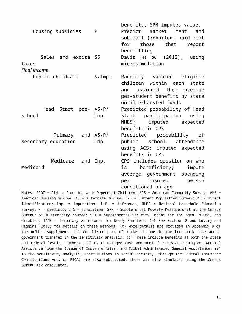
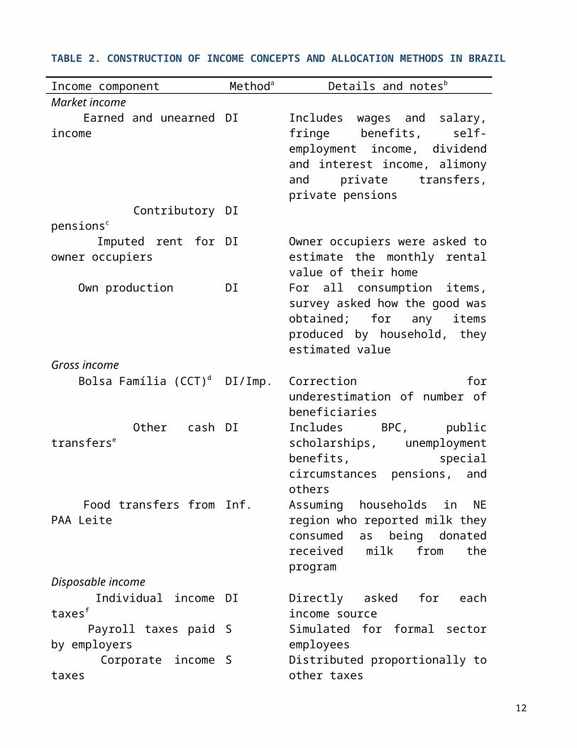
For our incidence analysis, we use definitions of five income concepts adapted from Lustig and Higgins (2013). Tables 1 and 2 summarize the allocation methods used for each income component in the two countries; further detail is provided in Appendix B of the online supplement.

TABLE 1. CONSTRUCTION OF INCOME CONCEPTS AND ALLOCATION METHODS IN THE UNITED STATES

Income component Methoda Details and notesb

Market income Earned and unearned income

DI Includes wages and salary, fringe benefits, dividend and interest income, farm and non-farm business income, alimony and private transfers, and worker’s compensation

Private scholarships Inf. Scholarship income greater than $5,550 (the maximum Pell Grant amount) was inferred to be from private scholarships

Contributory pensionsc DI Includes social security income, survivor’s benefits, and disability benefits

Imputed rent for owner occupiers

AS/P Predict rental value of owner occupiers’ homes using AHS and match to owner occupiers in CPS

Gross income SNAP (food stamps) DI/Imp. Correction for underestimation of

number of beneficiaries Cash transfersd DI Includes welfare and welfare-to-

work programs, TANF, AFDC, others, SSI, veterans’ benefits, unemployment insurance

Pell grants Inf. Scholarship income up to $5,550 (the maximum Pell Grant amount) was inferred to be from Pell Grants

EITC, CTC, MWP S Census Bureau tax calculator WIC and School Lunch Imp. CPS includes questions on

whether family is beneficiary; SPM imputes value.

Disposable income

7

Individual income taxese S Census Bureau tax calculator Corporate income taxes S Distributed proportionally to

other taxes Property taxes AS/DI AHSPost-fiscal income Heating subsidies Imp. CPS includes questions on

whether family received benefits; SPM imputes value.

Housing subsidies P Predict market rent and subtract (reported) paid rent for those that report benefitting

Sales and excise taxes SS Davis et al. (2013), using microsimulation

Final income Public childcare S/Imp. Randomly sampled eligible

children within each state and assigned them average per-student benefits by state until exhausted funds

Head Start pre-school AS/P/Imp.

Predicted probability of Head Start participation using NHES; imputed expected benefits in CPS

Primary and secondary education

AS/P/Imp.

Predicted probability of public school attendance using ACS; imputed expected benefits in CPS

Medicare and Medicaid Imp. CPS includes question on who is beneficiary; impute average government spending per insured person conditional on age

Notes: AFDC = Aid to Families with Dependent Children; ACS = American Community Survey; AHS = American Housing Survey; AS = alternate survey; CPS = Current Population Survey; DI = direct identification; imp. = imputation; inf. = inference; NHES = National Household Education Survey; P = prediction; S = simulation; SPM = Supplemental Poverty Measure unit at the Census Bureau; SS = secondary source; SSI = Supplemental Security Income for the aged, blind, and disabled; TANF = Temporary Assistance for Needy Families. (a) See Section 2 and Lustig and Higgins (2013) for details on these methods. (b) More details are provided in Appendix B of the online supplement. (c) Considered part of market income in the benchmark case and a government transfer in the sensitivity analysis. (d) These include benefits at both the state and federal levels. “Others” refers to Refugee Cash and Medical Assistance program, General Assistance from the Bureau of Indian Affairs, and Tribal Administered General Assistance. (e) In the sensitivity analysis, contributions to social security (through the Federal Insurance Contributions Act, or FICA) are also subtracted; these are also simulated using the Census Bureau tax calculator.

TABLE 2. CONSTRUCTION OF INCOME CONCEPTS AND ALLOCATION METHODS IN BRAZIL

Income component Methoda Details and notesb

Market income Earned and unearned income

DI Includes wages and salary, fringe benefits, self-employment income,

8

dividend and interest income, alimony and private transfers, private pensions

Contributory pensionsc DI Imputed rent for owner occupiers

DI Owner occupiers were asked to estimate the monthly rental value of their home

Own production DI For all consumption items, survey asked how the good was obtained; for any items produced by household, they estimated value

Gross income Bolsa Família (CCT)d DI/Imp. Correction for underestimation of

number of beneficiaries Other cash transferse DI Includes BPC, public

scholarships, unemployment benefits, special circumstances pensions, and others

Food transfers from PAA Leite

Inf. Assuming households in NE region who reported milk they consumed as being donated received milk from the program

Disposable income Individual income taxesf DI Directly asked for each income

source Payroll taxes paid by employers

S Simulated for formal sector employees

Corporate income taxes S Distributed proportionally to other taxes

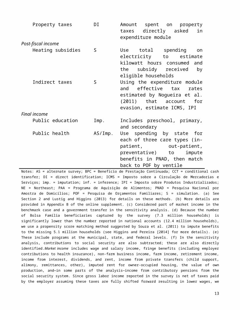
Property taxes DI Amount spent on property taxes directly asked in expenditure module

Post-fiscal income Heating subsidies S Use total spending on electricity

to estimate kilowatt hours consumed and the subsidy received by eligible households

Indirect taxes S Using the expenditure module and effective tax rates estimated by Nogueira et al. (2011) that account for evasion, estimate ICMS, IPI

Final income Public education Imp. Includes preschool, primary, and

secondary Public health AS/Imp. Use spending by state for each of

9

three care types (in-patient, out-patient, preventative) to impute benefits in PNAD, then match back to POF by ventile

Notes: AS = alternate survey; BPC = Benefício de Prestação Continuada; CCT = conditional cash transfer; DI = direct identification; ICMS = Imposto sobre a Circulação de Mercadorias e Serviços; imp. = imputation; inf. = inference; IPI = Imposto sobre Produtos Industrializados; NE = Northeast; PAA = Programa de Aquisição de Alimentos; PNAD = Pesquisa Nacional por Amostra de Domicílios; POF = Pesquisa de Orçamentos Familiares; S = simulation. (a) See Section 2 and Lustig and Higgins (2013) for details on these methods. (b) More details are provided in Appendix B of the online supplement. (c) Considered part of market income in the benchmark case and a government transfer in the sensitivity analysis. (d) Because the number of Bolsa Família beneficiaries captured by the survey (7.3 million households) is significantly lower than the number reported in national accounts (12.4 million households), we use a propensity score matching method suggested by Souza et al. (2011) to impute benefits to the missing 5.1 million households (see Higgins and Pereira [2014] for more details). (e) These include programs at the municipal, state, and federal levels. (f) In the sensitivity analysis, contributions to social security are also subtracted; these are also directly identified.Market income includes wage and salary income, fringe benefits (including employer contributions to health insurance), non-farm business income, farm income, retirement income, income from interest, dividends, and rent, income from private transfers (child support, alimony, remittances, other), imputed rent for owner-occupied housing, the value of own production, and—in some parts of the analysis—income from contributory pensions from the social security system. Since gross labor income reported in the survey is net of taxes paid by the employer assuming these taxes are fully shifted forward resulting in lower wages, we gross up market income by adding taxes paid by the employer. Similarly, we gross up market income in the case of corporate income taxes.8

With respect to contributory social security pensions, Lustig et al. (2014) explain that arguments exist for treating them as part of market income because they are deferred income similar to personal savings, as well as for treating them as a government transfer since there may not be a deterministic link between the amount contributed and the benefit received, and many systems run a deficit financed by general tax revenues. Hence, for a number of tables we present results under both scenarios: the scenario in which they are treated as part of market income (the “benchmark case”) and the one in which they are treated as a government transfer (the “sensitivity analysis”). In the benchmark case, we do not subtract contributions to social security out of income when moving from gross to disposable income because they are treated like any other form of personal savings. In the sensitivity analysis we do subtract out contributions, treating them as a tax. The results and comparison are sensitive to how contributory pensions are treated, which is unsurprising given Bourguignon et al.’s (2008) finding that a large portion of the difference in inequality in the two countries is due to the distribution of pensions.

In Brazil, all components of market income are directly identified in the survey. The value of goods produced for own consumption uses the expenditure component of POF, which includes questions about the way each good was obtained or purchased. Survey respondents must still report the value of goods that were obtained through own production or from the household’s business 8 For more detail on grossing up, see for example Alm et al. (1990) and Wallace et al. (1991).

10

inventory; we use the reported values. Imputed rent for owner occupied housing uses the responses to a survey question asking owner occupiers how much their dwelling would be rented for if it were rented.

In the US, the components of market income are directly identified in the survey with the exception of private scholarships and imputed rent. For private scholarships, we use the survey question on scholarship income and infer that scholarships greater than $5,550 (the maximum amount for Pell grants, a scholarship funded by the federal government) are private scholarships. For imputed rent for owner occupied housing, we predict rental values of owner occupiers’ homes using the AHS and match these values to owner occupiers in CPS. We do not include the value of own production in the US due to data limitations, but take solace in the fact that own production of food is very small in the US compared to Brazil, accounting for around 0.1 percent of GDP (USDA, 2014, Table 1).9

Gross income equals market income plus direct cash and food transfers. The economic incidence of these benefits is assumed to fall entirely on beneficiary households, and we ignore potential spillovers to other households. In the case of Brazil, direct cash transfers include the flagship anti-poverty conditional cash transfer (CCT) program Bolsa Família, the non-contributory pension program Benefício de Prestação Continuada (BPC), public scholarships, unemployment benefits, special circumstances pensions, and other direct transfers (including benefits from state and municipal level programs, such as São Paolo state’s Renda Cidadã CCT). Because benefits from these programs are directly identified, non-take up of benefits is not an issue (assuming survey reporting is accurate): we only attribute benefits to those who report receiving them in the survey. Milk transfers from the Programa de Aquisição de Alimentos (PAA) are inferred by assuming that households in the region of Brazil where the program operates who reported the milk they consumed as being donated received that milk from the program.

In the case of the US, direct cash transfers include welfare and welfare-to-work payments at the federal and state level, Temporary Assistance for Needy Families (TANF), Aid for Families with Dependent Children (AFDC), non-contributory pensions from the Supplemental Security Income (SSI) program, veterans’ benefits, unemployment benefits, Pell grants, and worker’s compensation. Near-cash and food transfer programs in the US include the Supplemental Nutrition Assistance Program (SNAP; more commonly known as “food stamps”), Special Supplemental Nutrition Program for Women, Infants, and Children (WIC), and

9 We do not attempt to value home production of services (e.g., time spent in child-rearing, caring for the sick and the elderly, house cleaning, cooking and other household chores) in either country.

11

free and reduced-price school lunches for low-income families. Benefits from all of the cash transfer programs, as well as SNAP, are directly identified10; the value of WIC and school lunches are imputed to households responding that the mother or children received benefits from the program. Since these benefits are, in all cases, based on a survey question identifying which households participate in the program, non-take up of benefits is accounted for to the extent that households who do receive benefits report them, and households do not erroneously report participating in the program.11 We also treat refundable tax credits—the federal and state Earned Income Tax Credit (EITC), federal Child Tax Credit (CTC), and federal Making Work Pay (MWP)—as direct transfers (and, hence, use pre-credit liabilities in the direct tax calculations).12 We account for non-take up of refundable tax credit benefits by only attributing benefits to eligible households in which at least one member reported filing a tax return in CPS (eligible households that file a tax return automatically receive benefits).

Disposable income equals gross income minus individual income taxes and payroll taxes (including those paid by the employer), corporate income taxes, and property taxes. Taxes at the federal, state, and local levels are included. Individual income taxes (including social security contributions) are assumed to be borne fully by labor in the formal sector, as are payroll taxes paid by the employer (which are borne by the formal labor sector in the form of lower wages). Corporate income taxes are assumed to fall partially on capital, and to be partially shifted forward to labor and consumers. Due to the theoretical and empirical uncertainty with respect to who bears the burden of the corporate income tax (Auerbach, 2006), this is a middle of the road approach. Property taxes are assumed to be borne fully by property owners.

In Brazil, individual income and property taxes paid are directly identified in the labor and expenditure modules of the survey, respectively; we simulate payroll taxes paid by employers and corporate income taxes. In the case of payroll taxes, we only simulate them for workers that we assume to be in the formal sector; since the survey lacks a question on whether a worker is in the formal sector, we assume that those who report paying income taxes are in the formal sector. Under the assumption that those working in the informal sector or shadow economy do not erroneously report paying taxes, our analysis of direct taxes thus takes into account the role of the shadow economy by only subtracting taxes for those in the formal sector. In the US, individual and corporate income taxes are simulated, while property taxes are identified in an alternate survey, the AHS,

10 With the exception of Pell grants, which were inferred.11 In both countries, we make a correction for the underestimation of the number of beneficiaries in our survey for the most effective anti-poverty programs for the non-elderly (Bolsa Família in Brazil and SNAP in the US). See Appendix B of the online supplement for more details.12 This is the same approach as that taken by the OECD (Denk et al., 2013).

12

and matched to households in the CPS. Our simulation of individual income taxes accounts for evasion by applying tax law only to households in which at least one member reported filing a tax return in CPS.

Post-fiscal income equals disposable income plus indirect subsidies minus indirect taxes. The indirect subsidies included in our analysis are housing and household energy subsidies targeted to low-income families. Allocating other government subsidies to individual households proved to be intractable. In Brazil, the main housing subsidy program Minha Casa Minha Vida was not implemented until late 2009, after the survey was completed; hence, we do not include it in our analysis. In the US, a variety of targeted housing subsidies exist, which are all included in the analysis because the CPS question on housing assistance is ambiguous enough to include all programs; the benefit is imputed by estimating the market value rent of the dwelling and subtracting the reported rent paid, which is asked of those who receive housing subsidies.

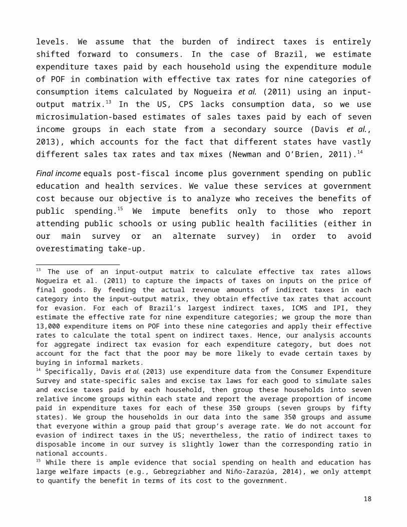
Energy subsidies come from Tarifa Social de Energia Elétrica (TSEE) in Brazil and Low-Income Home Energy Assistance (LIHEAP) in the US. Indirect taxes are expenditure taxes at both the federal and state levels. We assume that the burden of indirect taxes is entirely shifted forward to consumers. In the case of Brazil, we estimate expenditure taxes paid by each household using the expenditure module of POF in combination with effective tax rates for nine categories of consumption items calculated by Nogueira et al. (2011) using an input-output matrix.13 In the US, CPS lacks consumption data, so we use microsimulation-based estimates of sales taxes paid by each of seven income groups in each state from a secondary source (Davis et al., 2013), which accounts for the fact that different states have vastly different sales tax rates and tax mixes (Newman and O’Brien, 2011).14

13 The use of an input-output matrix to calculate effective tax rates allows Nogueira et al. (2011) to capture the impacts of taxes on inputs on the price of final goods. By feeding the actual revenue amounts of indirect taxes in each category into the input-output matrix, they obtain effective tax rates that account for evasion. For each of Brazil’s largest indirect taxes, ICMS and IPI, they estimate the effective rate for nine expenditure categories; we group the more than 13,000 expenditure items on POF into these nine categories and apply their effective rates to calculate the total spent on indirect taxes. Hence, our analysis accounts for aggregate indirect tax evasion for each expenditure category, but does not account for the fact that the poor may be more likely to evade certain taxes by buying in informal markets.14 Specifically, Davis et al. (2013) use expenditure data from the Consumer Expenditure Survey and state-specific sales and excise tax laws for each good to simulate sales and excise taxes paid by each household, then group these households into seven relative income groups within each state and report the average proportion of income paid in expenditure taxes for each of these 350 groups (seven groups by fifty states). We group the households in our data into the same 350 groups and assume that everyone within a group paid that group’s average rate. We do not account for evasion of indirect taxes in the US; nevertheless, the ratio of indirect taxes to disposable income in our survey is slightly lower than the corresponding ratio in national accounts.

13

Final income equals post-fiscal income plus government spending on public education and health services. We value these services at government cost because our objective is to analyze who receives the benefits of public spending.15 We impute benefits only to those who report attending public schools or using public health facilities (either in our main survey or an alternate survey) in order to avoid overestimating take-up.

In Brazil, unlimited free access to public health care facilities is guaranteed by the 1988 Constitution; because POF does not have data on who received health care at public facilities, we use an alternate survey: the 2008 PNAD, which has a detailed health supplement. Because spending on health services can vary in different geographic areas of a country, and because the amount of spending on different types of care can vary drastically, we follow the recommendation of O’Donnell et al. (2008) and take these into account to the extent possible. Specifically, from Brazil’s national health accounts (NHA) we obtain spending by state for each of three broad categories of health care: preventative care, basic care, and inpatient care. We then map the thirteen types of health services reported in PNAD into these three categories, and calculate the total number of visits for each category within each state according to PNAD. For each category-state pair, we divide total spending from NHA by total visits from PNAD to obtain per-visit spending, and impute this value to each reported visit for that type of care in that state in our microdata. In the United States, social spending on health care takes the form of the Medicare and Medicaid programs, which are imputed at their government cost to those who are covered by these public programs. Specifically, for each age (because spending varies significantly by age), we divide total government spending on Medicare for people of that age by the number of people of that age identified as insured by those programs in CPS, and allocate this age-specific benefit amount to each insured individual. We follow the same procedure for Medicaid.

Education benefits are allocated to individuals who report attending a public daycare, pre-school, primary, or secondary school, and are valued at the per-pupil government spending for that education level. Public daycare programs for low-income families (either in the form of free daycare centers or subsidy vouchers) exist in both countries; in the US they are funded by the Child Care Development Fund (CCDF) and TANF. Public pre-school is available (in theory) to all families in Brazil and to low-income families in the US, where it usually takes the form of participation in the Head Start program. Although tertiary education is free at all public universities in Brazil and highly subsidized at public universities in the US, the lack of data on who attends public universities in the US and the difficulty in 15 While there is ample evidence that social spending on health and education has large welfare impacts (e.g., Gebregziabher and Niño-Zarazúa, 2014), we only attempt to quantify the benefit in terms of its cost to the government.

14

allocating benefits led us to omit tertiary spending from our analysis for both countries.16 In Brazil, we obtain average per-pupil public education spending at each level (daycare, pre-school, lower primary, upper primary, and secondary) from the Ministry of Education and impute these benefits to students who report attending public school at that level.

In the United States, CPS does not include a question about whether students attended public or private school, so we combine alternate surveys with the prediction and imputation methods. Specifically, for primary and secondary education we use the ACS, which includes questions about income, student and household characteristics, and public vs. private school enrollment. We use a probit for the subsample that attended primary or secondary school to estimate the probability of choosing public school conditional on covariates common to both surveys. The coefficients from this regression were then applied to the same variables in the CPS data to estimate a probability of attending public school for each student who reported attending primary or secondary school. The probability of attending public school was multiplied by the average per-pupil spending in the student’s state—from Census Bureau (2012)—to calculate the expected public spending on education received by that student. We follow a similar procedure for Head Start using the NHES and restricting our probit to children ages 3–6. We again multiply the probability of receiving benefits from Head Start, predicted in CPS using coefficients from the NHES probit, by average per student spending by state, which was obtained from the Early Childhood Learning and Knowledge Center (2012).17 More details are available in Appendix B of the online supplement.

Each of these income concepts is aggregated at the household level and assumed to be shared equally among the members of the household (relative to their needs). If we assume no economies of scale within households, we would then divide household income by the number of people in the household and use household per capita income in the analysis. If we assume maximum economies of scale, so that the marginal cost of fulfilling the needs of any household member 16 For an attempt to make such an estimate in Europe, see Callan et al. (2008). Higgins and Pereira (2014) include tertiary spending in Brazil. 17 Note that in CPS we don’t know which students attended public school so we are not imputing the full value of per pupil spending to anyone; by multiplying each student’s predicted probability of attending public school by per pupil spending, we are assigning each student the expected value of the amount spent on him or her. As a check of our method, we verify that the average predicted probability from applying the coefficients of the ACS survey to CPS data is almost identical to the proportion of students attending public school (according to both ACS and administrative data). We also verify that total public spending on education using this method is approximately equal to total education spending in national accounts. For public childcare benefits, we follow a different approach: we compute average spending per beneficiary by state using the total program spending and number of beneficiaries from Office of Family Assistance (2012) for TANF child care and Office of Child Care (2013) for CCDF, then randomly sample eligible households within each state and assign them benefits until we have exhausted the funds.

15

after the first is zero, then we would simply use household aggregate income in the analysis. Equivalence scales account for some degree of economies of scale within households between these two extremes. Often, these scales vary across nations’ poverty and inequality estimates, and sometimes the assumptions made can take extreme forms (for instance, the World Bank generally uses household per capita incomes when estimating poverty, thereby assuming zero economies of scale within households).

There is no one scale that is commonly used in the US and Brazil, but there is one simple scale employed in most cross-national comparisons of income inequality (Johnson and Smeeding, forthcoming): the square root scale. This scale is a special case of the equivalence scales proposed by Buhmann et al. (1988), and was suggested by Atkinson et al. (1995). We apply this scale to both cash incomes (including cash benefits) and to public spending in education and health.18 Appendix A in the online supplement explores the robustness of our results to the choice of equivalence scale and presents results using household per capita and total household income.

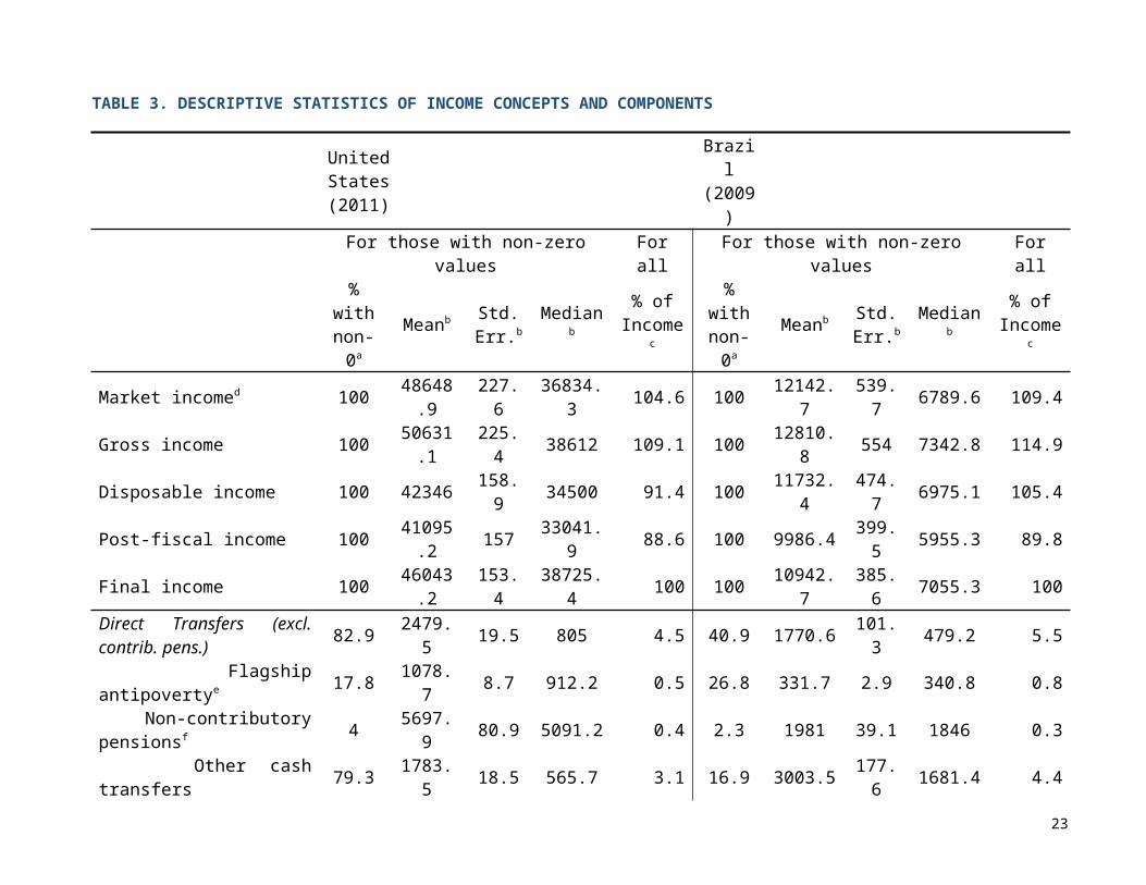
Table 3 provides descriptive statistics for each income component.

18 For a discussion of the merits of this approach and its alternative (applying the equivalence scale to cash income but not to public spending in education and health) see Garfinkel et al. (2006; 2010).

16

TABLE 3. DESCRIPTIVE STATISTICS OF INCOME CONCEPTS AND COMPONENTS

United States (2011)

Brazil (2009

)For those with non-zero values For all For those with non-zero values For all

% with non-0a

Meanb Std. Err.b

Medianb

% of Incom

ec

% with

non-0aMeanb Std.

Err.bMedia

nb

% of Incom

ec

Market incomed 100 48648.9 227.6 36834.

3 104.6 100 12142.7

539.7 6789.6 109.4

Gross income 100 50631.1 225.4 38612 109.1 100 12810.

8 554 7342.8 114.9

Disposable income 100 42346 158.9 34500 91.4 100 11732.4

474.7 6975.1 105.4

Post-fiscal income 100 41095.2 157 33041.

9 88.6 100 9986.4 399.5 5955.3 89.8

Final income 100 46043.2 153.4 38725.

4 100 100 10942.7

385.6 7055.3 100

Direct Transfers (excl. contrib. pens.) 82.9 2479.5 19.5 805 4.5 40.9 1770.6 101.

3 479.2 5.5 Flagship antipovertye 17.8 1078.7 8.7 912.2 0.5 26.8 331.7 2.9 340.8 0.8 Non-contributory pensionsf 4 5697.9 80.9 5091.2 0.4 2.3 1981 39.1 1846 0.3

Other cash transfers 79.3 1783.5 18.5 565.7 3.1 16.9 3003.5 177.6 1681.4 4.4

Food transfersg 31.1 867.7 9.1 280.6 0.6 1 109.8 5.5 79.5 0Direct Transfers (incl. contrib. pens.) 94.4 6276.1 37.7 2250.7 11.8 57.7 4312.6 227.

3 2104 19.9 Contributory pensions 26.1 13567.

6 68.8 12714.5 7.3 27.6 5872.4 300.

5 3362.7 14.4Direct Taxes (excl. contributions)h 100 -

8293.6 71.8 -3941.1 -17.8 100 -

1078.5 90.6 -260.9 -9.5

17

Individual income and payrollh 76.2 -

8380.4 81.4 -4379.1 -13.5 47.7 -

1443.2127.

5 -458.5 -6.7 Corporate 100 -755.6 5.6 -424.3 -1.6 100 -174.4 9.8 -80.9 -1.6 Property 57.8 -

2209.9 21.9 -1386.6 -2.7 25.1 -423.3 42.7 -121.5 -1.2

Direct Taxes (incl. contributions)h 100

-10780.

380.2 -

5898.3 -23.2 100 -1277.4

102.6 -272.5 -11.4

Contributions to social security 79.6 -

3237.5 12.8 -2678 -5.5 10.9 -1660.6

112.6 -540.9 -1.8

Indirect taxes and subsidies 100 -

1250.5 4.3 -1311.5 -2.8 100 -

1746.2 75.6 -1005.2 -15.6

Heating and housing subs. 7 1971.8 33.2 1085.4 0.2 32.1 33 0.4 28.9 0.1 Sales and excise taxes 100 -

1372.9 2.8 -1317.6 -3 100 -

1755.6 75.4 -1015.7 -15.7

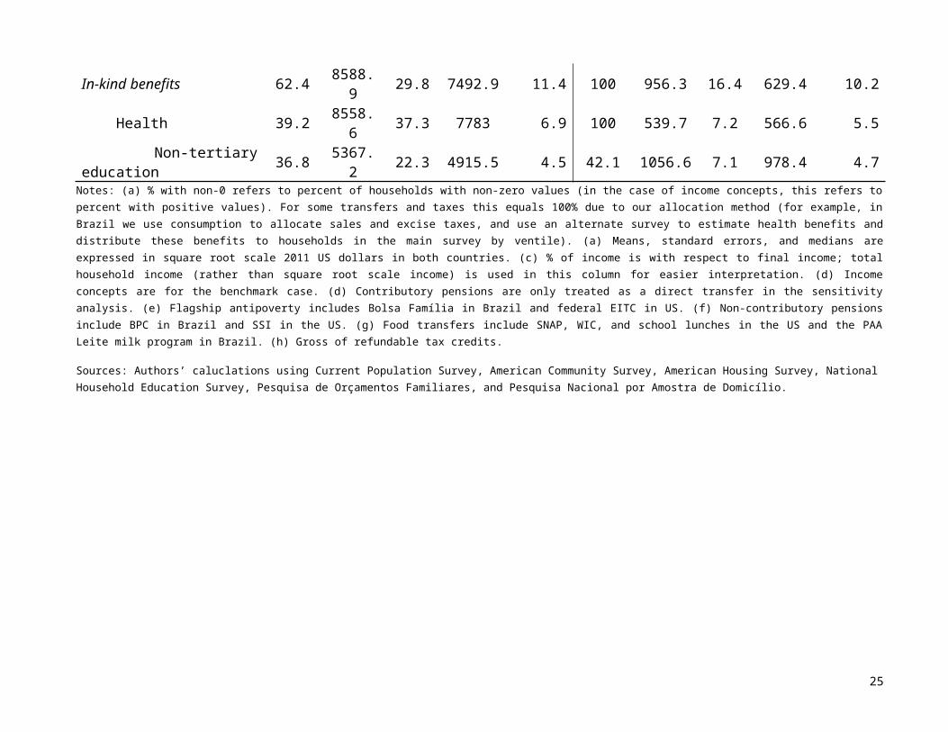
In-kind benefits 62.4 8588.9 29.8 7492.9 11.4 100 956.3 16.4 629.4 10.2 Health 39.2 8558.6 37.3 7783 6.9 100 539.7 7.2 566.6 5.5 Non-tertiary education 36.8 5367.2 22.3 4915.5 4.5 42.1 1056.6 7.1 978.4 4.7

Notes: (a) % with non-0 refers to percent of households with non-zero values (in the case of income concepts, this refers to percent with positive values). For some transfers and taxes this equals 100% due to our allocation method (for example, in Brazil we use consumption to allocate sales and excise taxes, and use an alternate survey to estimate health benefits and distribute these benefits to households in the main survey by ventile). (a) Means, standard errors, and medians are expressed in square root scale 2011 US dollars in both countries. (c) % of income is with respect to final income; total household income (rather than square root scale income) is used in this column for easier interpretation. (d) Income concepts are for the benchmark case. (d) Contributory pensions are only treated as a direct transfer in the sensitivity analysis. (e) Flagship antipoverty includes Bolsa Família in Brazil and federal EITC in US. (f) Non-contributory pensions include BPC in Brazil and SSI in the US. (g) Food transfers include SNAP, WIC, and school lunches in the US and the PAA Leite milk program in Brazil. (h) Gross of refundable tax credits.

Sources: Authors’ caluclations using Current Population Survey, American Community Survey, American Housing Survey, National Household Education Survey, Pesquisa de Orçamentos Familiares, and Pesquisa Nacional por Amostra de Domicílio.

18

iv Limitations

Although the implementation of a consistent methodology aspires to achieve a high degree of comparability, survey differences can compromise this comparability. The sampling between the two primary surveys differ, such that POF is representative at the state level but CPS is not; the latter fact means our estimations of consumption and property taxes in the US—which take into account the largely different tax mixes of each state—are imperfect. The survey designs also differ: in the case of imputed rent for owner occupied housing, for example, POF asks owner occupiers how much their dwelling would be rented for if it were rented, while CPS only identifies who owns their home and even lacks data on rates paid by renters (which rules out the usual regression technique to predict imputed rent). Thus, we follow the methodology of Short and O’Hara (2008), which involves predicting rental rates using a matching technique with the AHS. It was also not possible to account for the value of own food production in the CPS; however, we still accounted for it in Brazil given its relatively higher importance there.

By restricting our analysis to taxation and social spending, we overlook government spending on public sector wages. Although higher public sector employment is associated with lower inequality on a global level (Milanović, 1994), public sector wages are regressive in Brazil (Medeiros and Souza, 2013). Public servants in both countries earn a wage premium over comparable private sector workers. In Brazil, this premium has been increasing over time (Souza and Medeiros, 2013), while it has been decreasing in the US (Borjas, 2002); in addition, the levels and trends of the public-private wage differential differ substantially by education level (Poterba and Rueben, 1994, Braga et al., 2009). Our analysis makes no attempt to capture this aspect of public spending, which could dampen the redistributive impact of the state.

Our results for final income and the imputations of public health and education benefits must be analyzed with the following perspectives in mind. First, the middle and upper classes might opt out of public education and health services due to quality concerns (Ferreira et al., 2013) which would inflate inequality reduction relative to the counterfactual where the middle and upper classes also use public services. Second, spending amounts do not necessarily reflect quality (which comes into play in both the US with respect to inflated healthcare costs

19

and in Brazil with respect to low quality services).19 Third, although we account for differences in per student spending by state, using state spending averages still overlooks the large intrastate variations of spending across localities and the fact that—unlike other OECD countries—the US spends somewhat less on students from disadvantaged backgrounds than on other students (OECD, 2011b, Wilson et. al., 2006).

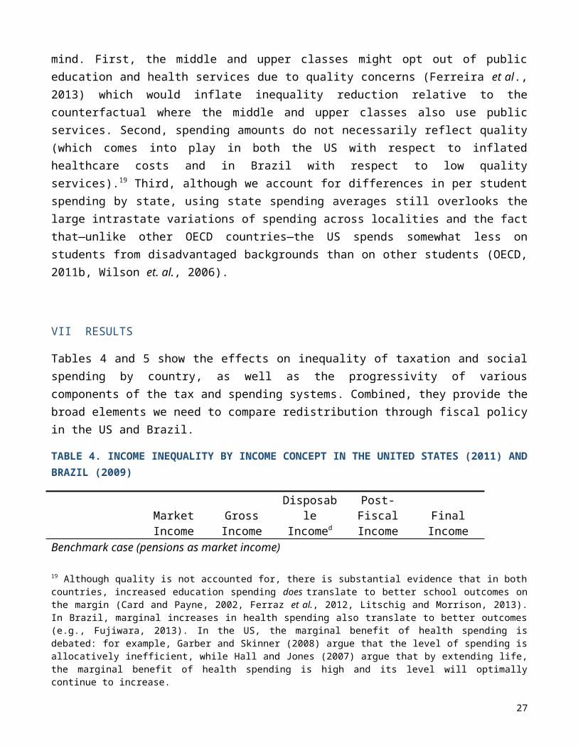
3 RESULTS

Tables 4 and 5 show the effects on inequality of taxation and social spending by country, as well as the progressivity of various components of the tax and spending systems. Combined, they provide the broad elements we need to compare redistribution through fiscal policy in the US and Brazil.

TABLE 4. INCOME INEQUALITY BY INCOME CONCEPT IN THE UNITED STATES (2011) AND BRAZIL (2009)

Market Income

GrossIncome

Disposable Incomed

Post-Fiscal

IncomeFinal

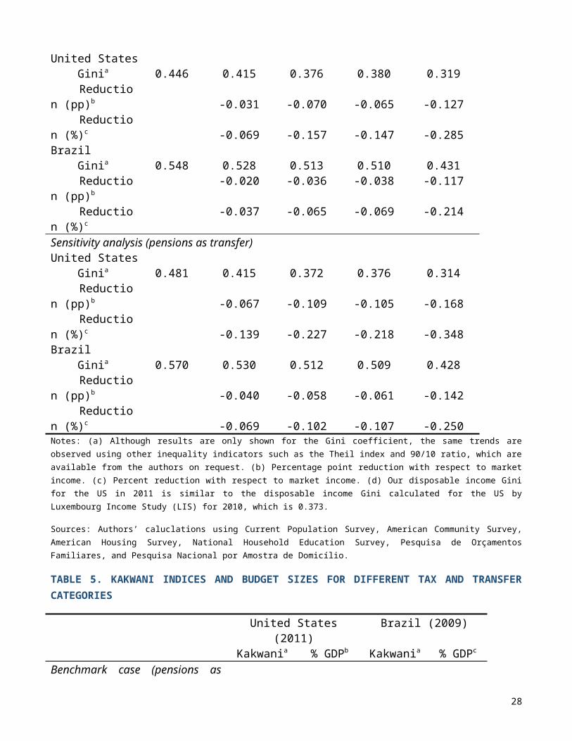
IncomeBenchmark case (pensions as market income)United States Ginia 0.446 0.415 0.376 0.380 0.319 Reduction (pp)b -0.031 -0.070 -0.065 -0.127 Reduction (%)c -0.069 -0.157 -0.147 -0.285Brazil Ginia 0.548 0.528 0.513 0.510 0.431 Reduction (pp)b

-0.020 -0.036 -0.038 -0.117

Reduction (%)c

-0.037 -0.065 -0.069 -0.214

Sensitivity analysis (pensions as transfer)United States Ginia 0.481 0.415 0.372 0.376 0.314 Reduction (pp)b -0.067 -0.109 -0.105 -0.16819 Although quality is not accounted for, there is substantial evidence that in both countries, increased education spending does translate to better school outcomes on the margin (Card and Payne, 2002, Ferraz et al., 2012, Litschig and Morrison, 2013). In Brazil, marginal increases in health spending also translate to better outcomes (e.g., Fujiwara, 2013). In the US, the marginal benefit of health spending is debated: for example, Garber and Skinner (2008) argue that the level of spending is allocatively inefficient, while Hall and Jones (2007) argue that by extending life, the marginal benefit of health spending is high and its level will optimally continue to increase.

20

Reduction (%)c -0.139 -0.227 -0.218 -0.348Brazil Ginia 0.570 0.530 0.512 0.509 0.428 Reduction (pp)b -0.040 -0.058 -0.061 -0.142 Reduction (%)c -0.069 -0.102 -0.107 -0.250Notes: (a) Although results are only shown for the Gini coefficient, the same trends are observed using other inequality indicators such as the Theil index and 90/10 ratio, which are available from the authors on request. (b) Percentage point reduction with respect to market income. (c) Percent reduction with respect to market income. (d) Our disposable income Gini for the US in 2011 is similar to the disposable income Gini calculated for the US by Luxembourg Income Study (LIS) for 2010, which is 0.373.

Sources: Authors’ caluclations using Current Population Survey, American Community Survey, American Housing Survey, National Household Education Survey, Pesquisa de Orçamentos Familiares, and Pesquisa Nacional por Amostra de Domicílio.

TABLE 5. KAKWANI INDICES AND BUDGET SIZES FOR DIFFERENT TAX AND TRANSFER CATEGORIES

United States (2011) Brazil (2009)Kakwania % GDPb Kakwania % GDPc

Benchmark case (pensions as market income)

Direct Transfers(excluding contributory pensions)

0.741 3.32 0.582 4.16

Public Spending on Non-Tertiary Education and Healthd

0.671 10.49 0.747 9.32

Indirect Subsidies(heating and housing)e 1.292 0.26 0.938 0.05

Social Spending in Analysis(excluding contributory pensions)

0.699 14.07 0.696 13.53

Direct Taxes (federal, state, and local individual, corporate, and property)

0.179 14.74 0.165 8.17

Indirect Taxes (federal, state, and local expenditure taxes) -0.293 3.61 -0.031 12.90

All Taxes in Analysis(excluding contributions to

pensions)0.108 18.35 0.042 21.04

Sensitivity analysis (pensions as transfer)

Direct Transfers(including contributory pensions)

0.749 8.08 0.482 13.22

21

Public Spending on Non-Tertiary Education and Healthd

0.739 10.49 0.730 9.32

Indirect Subsidies(heating and housing)e 1.308 0.26 0.952 0.05

Social Spending in Analysis(including contributory pensions)

0.749 18.83 0.579 22.59

Direct Taxes and Contributions (federal, state, and local)

0.104 20.90 0.122 15.29

Indirect Taxes (federal, state, and local expenditure taxes) -0.347 3.61 -0.087 12.90

All Taxes and Contributions in Analysis 0.050 24.50 0.009 28.16

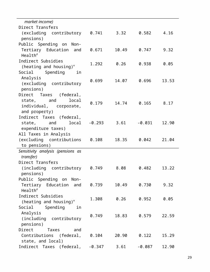
Notes: (a) The Kakwani coefficient is defined for taxes as the tax’s concentration coefficient minus the market income Gini. For transfers it is defined as the market income Gini minus the transfer’s concentration coefficient, so that a positive Kakwani always indicates progressivity. In the benchmark case, Kakwani coefficients are calculated with respect to benchmark case market income (which includes contributory pensions). In the sensitivity analysis, Kakwani coefficients are calculated with respect to sensitivity analysis market income (which does not include contributory pensions because they are treated as a government transfer). (b)-(c) Spending totals as a percent of GDP only include those taxes and transfers that are included in the analysis. (d) Non-tertiary education is the sum of public day care, preschool, primary, and secondary education spending. In Brazil, administrative education costs are listed as a separate line item, so we allocate them proportionally to each category of education spending. (e) Brazil’s subsidized housing program Minha Casa Minha Vida was not included because it was implemented in late 2009, after the household survey was completed.

Sources: (a) Authors’ calculations using Current Population Survey, American Community Survey, American Housing Survey, National Household Education Survey, Pesquisa de Orçamentos Familiares, and Pesquisa Nacional por Amostra de Domicílio. (b) Department of Health and Human Services’ Administration for Children and Families, Department of Commerce’s Bureau of Economic Analysis and Census Bureau, Department of Agriculture’s Food and Nutrition Service, Department of Education budget overview, and Department of the Treasury’s Internal Revenue Service. More detail on the source of each spending number is available in the online supplement. (c) Controladora Geral da União, Ministério da Agricultura Pecuária e Abastecimento, Ministério do Desenvolvimento Social e Combate à Fome, Ministério da Previdência e Assistência Social, Ministério do Trabalho, Secretaria de Avaliação e Gestão da Informação, Secretaria do Desenvolvimento Social do Governo do Estado de São Paulo, Secretaria do Tesouro Nacional.

i Direct Cash and Food Transfers

If we consider the impact of just direct transfers, the US reduces the Gini coefficient from 0.446 to 0.415, or by three percentage points or seven percent

22

(Table 4).20 Brazil has a much higher market income Gini than the US of 0.548, and reduces inequality by even less than the US with direct transfers, to a gross income Gini of 0.528, or by two percentage points (3.7 percent). Why does Brazil achieve less redistribution than the United States through direct cash and food transfers, despite spending a larger share of GDP on direct transfers? Even when including the relatively large refundable tax credits and food assistance programs such as the Supplemental Nutrition Assistance Program (SNAP) in the total for direct transfers, the US spends 3.3 percent of GDP on direct transfers, compared to 4.2 percent in Brazil. This difference is even more pronounced if contributory pensions are considered a government transfer, in which case the US spends 8.1 percent of GDP compared to 13.2 percent in Brazil. However, transfer spending is much more progressive in the US: the Kakwani index21 for direct transfers in the US is 0.741 (0.749) while in Brazil it equals 0.582 (0.482) when pensions are not (are) counted as a government transfer (Table 5).

Furthermore, every direct income transfer program in the US except Social Security pensions (if the latter are considered a government transfer) is progressive in absolute terms—i.e., the per capita transfer decreases with income. In contrast, in Brazil the larger direct transfer programs are progressive only in relative terms—that is, benefits as a proportion of income, but not per capita benefits, decrease with income. This can be seen in Tables 6 and 7, where the concentration coefficients for all direct transfer programs in the US except contributory pensions are negative, while they are positive (but less than the market income Gini, indicating that they are still equalizing) for some programs in Brazil.

20 Reductions in inequality could be measured in terms of absolute (percentage point) Gini reductions or relative (percent) reductions. From a social welfare perspective, percentage point reductions could be preferred due to their parallel with the Gini social welfare function (Duclos and Araar, 2006). Furthermore, measures of redistributive effect generally measure absolute changes (see, e.g., Lambert, 2001). On the other hand, if we consider the simplified scenario of a proportional tax and lump-sum transfer, the absolute Gini reduction is a function of the pre-tax pre-transfer Gini, while the relative Gini reduction is independent of the initial Gini (Luebker, 2014). Table 4 presents both absolute and relative reductions; in the text we mainly focus on absolute reductions.21 Note that the index originally proposed by Kakwani (1977) only measures the progressivity of taxes. It is defined as the tax’s concentration coefficient minus the market income Gini. To adapt to the measurement of transfers, Lambert (1985) suggests that in the case of transfers it should be defined as market income Gini minus the concentration coefficient (i.e., the negative of the definition for taxes) to make the index positive whenever the change is progressive. Also note that in the case of transfers, the Kakwani index can exceed unity (Lambert, 2001). Hence, a negative Kakwani indicates a regressive tax or transfer, while a positive Kakwani indicates a progressive tax or transfer; the index is higher the more progressive the tax or transfer. In the case of transfers, a Kakwani that is both positive and higher than the market income Gini indicates that the transfer is progressive in absolute terms—in other words, the absolute benefit decreases with income—while a Kakwani that is positive and less than the market income Gini indicates that the transfer is progressive in only relative terms—that is, the benefit as a proportion of income (but not the absolute benefit) decreases with income.

23

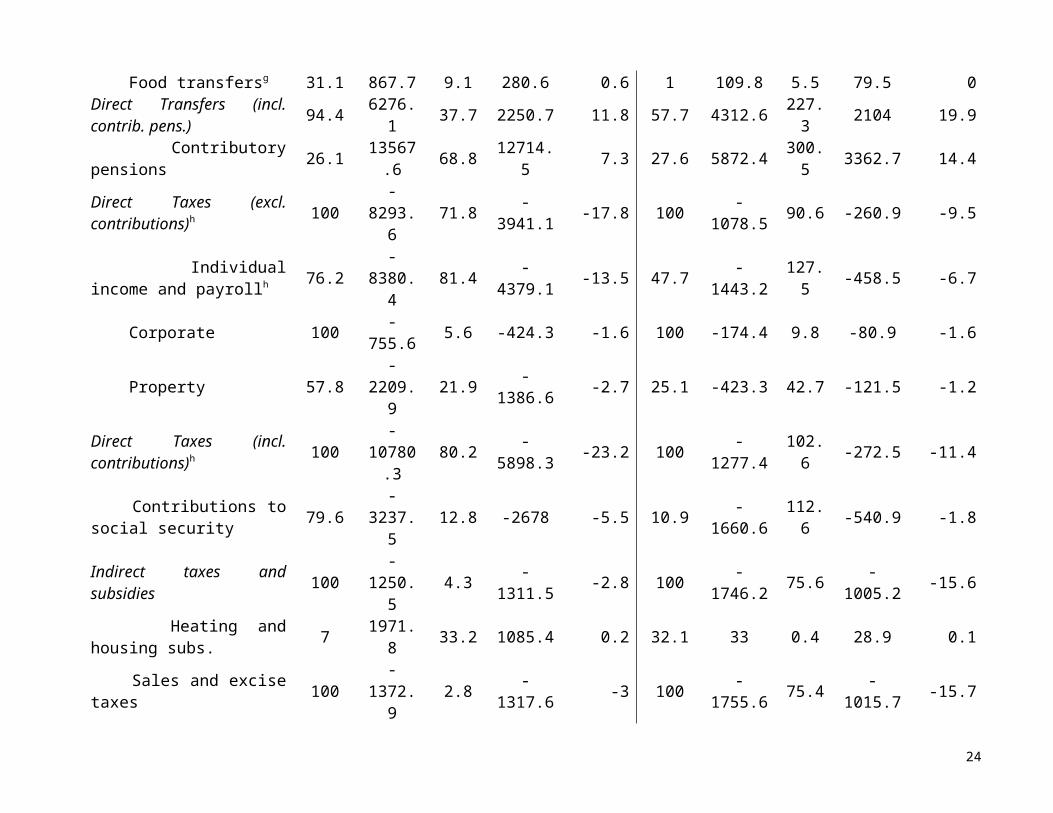
TABLE 6. CONCENTRATION COEFFICIENTS OF TRANSFERS PROGRAMS AND THEIR SIZE, UNITED STATES 2011

Concentration coefficient Program size

Program

w.r.t. benchmark case market

income

w.r.t. sensitivity analysis market income

in billions of US dollars

as a percent of

GDP

Total Social Spending including Pensionsa -0.182 -0.268 2822.9 18.83

Total Social Spending excluding Pensionsa -0.253 -0.267 2109.6 14.07

Direct Transfers including Pensionsb -0.120 -0.267 1210.9 8.08

Total Health Spendingc -0.307 -0.416 949.0 6.33Contributory Pensions

(SS) 0.018 -0.271 713.3 4.76Total Non-Tertiary

Education Spendingd -0.134 -0.082 623.9 4.16Primary and Secondary

Education -0.124 -0.072 602.6 4.02

Medicare -0.106 -0.317 545.1 3.64Direct Transfers

excluding Pensionse -0.295 -0.262 497.6 3.32

Medicaid -0.527 -0.523 403.9 2.69Unemployment Benefits -0.213 -0.177 108.0 0.72SNAP (food stamps) -0.721 -0.673 72.7 0.49Veteran’s Benefits -0.093 -0.221 63.6 0.42Federal EITC -0.566 -0.476 62.9 0.42SSI for aged, blind,

disabled (non-contributory pension)

-0.627 -0.620 50.4 0.34

Pell Grants -0.204 -0.154 34.8 0.23Housing Subsidies -0.858 -0.836 34.2 0.23State EITC -0.623 -0.554 24.8 0.17Welfare, TANF, AFDC -0.767 -0.725 21.1 0.14Worker's Compensation -0.085 -0.131 15.8 0.11Public Childcare -0.264 -0.195 13.7 0.09School Lunch -0.508 -0.439 10.1 0.07Head Start -0.708 -0.639 7.6 0.05WIC -0.628 -0.548 4.9 0.03Energy Subsidies -0.720 -0.714 4.8 0.03Federal CTC -0.133 -0.065 3.4 0.02Note: AFDC = Aid to Families with Dependent Children. CTC = Child Tax Credit. EITC = Earned Income Tax Credit. GDP = Gross Domestic Product. SNAP = Supplemental Nutrition Assistance Program. SS = Social Security. SSI = Supplemental Security Income. TANF = Temporary Assistance for Needy Families. w.r.t. =

24

with respect to. Programs are listed from largest to smallest. Market incomes and transfers are measured in equivalized terms using the square root scale. (a) Total social spending including (excluding) pensions is composed of direct transfers including (excluding) pensions, total health spending, total non-tertiary education spending, energy subsidies, and housing subsidies. (b) Direct transfers including pensions is composed of direct transfers excluding pensions and contributory pensions (SS). (c) Total health spending is composed of Medicare and Medicaid. (d) Total non-tertiary education spending is composed of primary and secondary education, Head Start, and public childcare. Tertiary education is not included in our analysis. (e) Direct transfers excluding pensions is composed of welfare, TANF, AFDC, SSI, Pell grants, veterans’ benefits, unemployment benefits, worker’s compensation, SNAP, WIC, school lunch, federal EITC, federal CTC, state EITC, and the Making Work Pay refundable tax credit.

Sources: Concentration coefficients are authors’ calculations using Current Population Survey, American Community Survey, American Housing Survey, and National Household Education Survey. Program sizes are from the Department of Health and Human Services’ Administration for Children and Families, Department of Commerce’s Bureau of Economic Analysis and Census Bureau, Department of Agriculture’s Food and Nutrition Service, and Department of Education budget overview.

TABLE 7. CONCENTRATION COEFFICIENTS OF TRANSFERS PROGRAMS AND THEIR SIZE, BRAZIL 2009

Concentration coefficient Program size

Program

w.r.t. benchmark case market

income

w.r.t. sensitivity analysis market income

in billions of US

dollarsg

as a percent of GDP

Total Social Spending including Pensionsa 0.152 -0.010 420.4 22.59

Total Social Spending excluding Pensionsa -0.149 -0.140 251.8 13.53

Direct Transfers including Pensionsb 0.380 0.088 246.0 13.22

Contributory Pensions 0.545 0.161 168.6 9.06Total Health Spending -0.125 -0.107 97.0 5.21Direct Transfers

excluding Pensionsc -0.033 -0.092 77.3 4.16Total Non-Tertiary

Education Spendingd -0.277 -0.216 76.4 4.11Primary Education -0.287 -0.226 59.4 3.19Special Circumstances

Pensionse 0.121 0.008 42.4 2.28Unemployment 0.152 0.213 10.9 0.58BPC (non-contributory

pensions) -0.479 -0.488 9.9 0.53Secondary Education -0.179 -0.134 9.5 0.51Public Childcaref -0.266 -0.193 7.6 0.41Preschoolf -0.328 -0.258Bolsa Família (CCT) -0.560 -0.492 7.3 0.39Other Direct Transfers 0.121 0.176 4.8 0.26Scholarships 0.252 0.285 2.1 0.11

25

Energy Subsidies -0.390 -0.382 1.0 0.05Milk Transfers -0.407 -0.372 0.1 0.01Note: BPC = Benefício de Prestação Continuada. CCT = Conditional Cash Transfer. GDP = Gross Domestic Product. Programs are listed from largest to smallest. Market incomes and transfers are measured in equivalized terms using the square root scale, which explains the differences between these concentration coefficients and those in Higgins and Pereira (2014). (a) Total social spending including (excluding) pensions is composed of direct transfers including (excluding) pensions, total health spending, total non-tertiary education spending, energy subsidies, and housing subsidies. Brazil’s main housing subsidy program, Minha Casa Minha Vida, was not included in the analysis because it was implemented in late 2009 after the household survey was completed. (b) Direct transfers including pensions is composed of direct transfers excluding pensions and contributory pensions. (c) Direct transfers excluding pensions is composed of Bolsa Família, BPC, scholarships, unemployment benefits, special circumstances pensions, milk transfers, and other direct transfers. (d) Total non-tertiary education spending includes public daycare and pre-school, primary, and secondary education. Administrative costs are a separate line item in Brazil, so they are distributed proportionally to each education category (including tertiary which is not included in our analysis). (e) These are considered a non-contributory pension for reasons described in Higgins and Pereira (2014). (f) The budgets for public childcare and preschool are combined in public accounts. (g) Conversion to US dollars uses the consumption-based purchasing power parity (PPP) adjusted exchange rate for 2009.

Sources: Concentration coefficients are authors’ calculations using Pesquisa de Orçamentos Familiares and Pesquisa Nacional por Amostra de Domicílio. Program sizes are from Controladora Geral da União, Ministério da Agricultura Pecuária e Abastecimento, Ministério do Desenvolvimento Social e Combate à Fome, Ministério da Previdência e Assistência Social, Ministério do Trabalho, Secretaria de Avaliação e Gestão da Informação, Secretaria do Desenvolvimento Social do Governo do Estado de São Paulo, Secretaria do Tesouro Nacional. One reason Brazil is not able to achieve more redistribution through direct transfers is that its highly progressive programs—such as its flagship CCT Bolsa Família, non-contributory pension program for the elderly poor BPC, and milk transfer program—are small: combined, the three programs make up less than 1 percent of GDP. Even for the poorest 10 percent of the population, they only increase market income by 29.4 percent, 11.0 percent, and a paltry 0.2 percent, respectively.22 This can be compared to the United States where the Supplemental Security Income program for the aged, blind, and disabled increases the market incomes of the bottom decile by 28.9 percent on average, while (the monetized values of) food assistance transfers (SNAP, WIC, and the school lunch program) increase their incomes by 38.6 percent.

Meanwhile, the majority of Brazil’s larger transfer programs, such as unemployment benefits, are progressive only in relative terms (Table 7)—that is, the ratio of transfer to income declines with income, but the absolute value of the transfer does not decline with income. The effect of these large and only relatively progressive programs on the redistributive impact of direct transfers can be seen in the concentration curve for direct transfers (the solid dark gray curve) in Figure 1: it begins concave and above the 45 degree line due to well-targeted programs like Bolsa Família, but then becomes convex and crosses the 45 degree line due to the larger less progressive programs. In fact, if contributory pensions are considered a government transfer, total direct transfers are progressive in relative terms only (as seen by the fact that their concentration coefficient is

22 Part of the reason that the non-contributory pension program only increases incomes of the poorest decile by 11 percent could be that recipients of the non-contributory pension program are not aware what program they received benefits from and hence do not report benefits from this program. Indeed, only 40 percent of the total number of beneficiaries according to administrative records were identified in the 2004 PNAD, which had a special supplement that asked three questions specifically about BPC (Soares et al., 2007).

26

positive but less than the market income Gini in Table 7): the better off benefit more in absolute terms from direct transfers than the poor.

FIGURE 1. CONCENTRATION CURVES FOR TAX AND SPENDING CATEGORIES (BENCHMARK CASE), BRAZIL 2009

Source: Authors’ elaboration using Pesquisa de Orçamentos Familiares and Pesquisa Nacional por Amostra de Domicílio.It is worth noting that the US was an economy in recovery in 2011, with an adult employment to population ratio still three percentage points below pre-recession levels (Kenworthy and Smeeding, 2014) and a budget deficit larger than before the recession (Congressional Budget Office, 2013). These circumstances likely increased the amount of redistribution observed, especially given the countercyclical nature of transfer programs such as food stamps (Ziliak, 2013).

ii Direct Taxes

Direct taxes reduce the Gini in the US by another four percentage points when moving from gross income to disposable income, compared to a two percentage point reduction in Brazil (Table 4). The discrepancy is slightly larger when pensions are treated as a government transfer (and hence contributions to the pension system are treated as a tax). Because the order that taxes and transfers are analyzed is somewhat arbitrary and the relative contribution of each to inequality reduction can be sensitive to the order chosen (Kim and Lambert, 2009), we also test the sensitivity of our comparisons of the redistributive effect

27

of taxes and transfers in the two countries to adopting the opposite order and first subtracting taxes from market income to arrive at net market income. The net market income benchmark case Ginis for the US and Brazil are 0.414 and 0.534, respectively, meaning that under this alternate path, direct taxes reduce the Gini coefficient by 3.1 percentage points in the US and 1.5 percentage points in Brazil.

Throughout Latin America, the individual income tax is underutilized as a revenue collection and redistributive tool (Corbacho et al., 2013). Direct taxes in Brazil are both smaller and less progressive than in the US. In Brazil, revenues from individual income taxes (at the federal, state, and local levels) only amount to 2.1 percent of GDP, compared to 9.3 percent for individual income taxes (at the federal, state, and local levels) in the US. Total direct taxes analyzed in this study—including individual income, corporate income, and property taxes at the federal, state, and local levels—are 14.7 percent of GDP in the US and 8.2 percent in Brazil. Furthermore, direct taxes are more progressive in the US: the Kakwani index (which measures the progressivity of a tax based on its concentration in the income distribution and is independent of the tax’s size) is 0.179 in the US, compared to 0.165 in Brazil (Table 2).

High levels of informality in Brazil may limit its ability to increase revenue collection from the individual income tax, considering that around 50 percent of Brazilian workers are informal and Brazil already collects personal income taxes at levels comparable to other middle-income countries (Corbacho et al., 2013). While some assume that the income tax’s existence per se encourages informality, the evidence on whether personal income taxes have increased informality in Latin America is mixed (Lora and Fajardo, 2012a); furthermore, the benefits of evasion are diminished in a general equilibrium framework (Alm and Sennoga, 2010), possibly to zero (Alm and Finlay, 2013). Two likely causes of Brazil’s persistent informality are that labor productivity has not increased at the same pace as minimum wages and contribution requirements, and that the effective rate on capital is significantly lower than that on labor, which can discourage firms from creating labor-intensive employment in the formal sector (Lora and Fajardo, 2012b).

Non-contributory pension programs and CCTs can also be double-edged swords by encouraging informality. Evidence exists that these programs have increased informality in Argentina (Garganta and Gasparini, 2012), Colombia (Camacho et al., 2013), and Mexico (Bosch and Campos, 2010). In Brazil, per-beneficiary non-contributory pension benefits are larger than in any other Latin American country; these large benefits could discourage formal employment by reducing the relative benefits of enrollment in the contributory pension system (Levy and Schady, 2013).

28

An additional factor working against Brazil is that the higher initial income inequality is—and it is much higher in Brazil than in the US—the more difficult it is to reduce income inequality through progressive taxes and transfers (Engel et al., 1999).

To put our results for redistribution using direct taxes and transfers into international perspective, we compare the US to EU countries in an analysis that broadly follows the same methodology (EUROMOD, 2014), and Brazil to other developing countries that also follow Lustig and Higgins’ (2013) methodology. When pensions are considered part of market income, the direct tax and transfer system in the US is more redistributive than some EU-27 countries (six Eastern European countries, as well as Italy, Greece, Cyprus, and Malta) but less redistributive than most. The eight European countries with the largest redistribution through direct taxes and transfers reduce their Gini coefficients by between ten and twenty-five percentage points—compared to seven percentage points in the US.23 When pensions are considered a government transfer, the direct tax and transfer system in the US is less redistributive than all EU-27 countries. This result is robust to comparisons with other rich countries and EU results from other studies (e.g., Morelli et al., forthcoming).24 We compare Brazil to studies for Armenia, Bolivia, Costa Rica, El Salvador, Ethiopia, Guatemala, Indonesia, Jordan, Mexico, Peru, South Africa, Sri Lanka, and Uruguay that also follow the Lustig and Higgins (2013) methodology.25 Brazil redistributes more through direct taxes and transfers than all of these countries except South Africa and Uruguay, which reduce inequality by 7.7 and 3.5 percentage points, respectively.

Compared to previous studies on Brazil and the US (e.g., Immervoll et al., 2009, Kim and Lambert, 2009), we find higher levels of redistribution due to direct taxes and transfers. This is likely due to both the comprehensiveness of our analysis (including, for example, food transfers, corporate income taxes, and payroll taxes paid by the employer) as well as the more recent years used in our

23 The comparison with the EU countries uses EUROMOD (2014) who also broadly follow the same methodology (specifically, we calculate the reduction between the “original income plus pensions”—which we call benchmark case market income—Gini and the disposable income Gini for each country in 2011). Moreover, the USA has the third highest market income inequality in comparison to the 27 EU nations. 24 These findings comparing our results to redistributive findings for European countries are consistent with studies that directly compare the US and Europe (e.g., Brandolini and Smeeding, 2009, Morelli et al., forthcoming). The lack of inequality reduction in the US is attributed to the very small amount of its resources dedicated to cash and near-cash transfers for the nonelderly. The US spends less than half of the relative amount spent in Canada and the UK, and less than a fourth of that spent in Sweden and Finland (Smeeding, 2005).25 We use our per capita results (available in Appendix A) rather than square root scale results for consistency with these studies. The references for these studies are Beneke et al. (2014), Bucheli et al. (2014), Cabrera et al. (2014), Jaramillo (2014), Lustig (2014), Paz Arauco et al. (2014), Sauma and Trejos (2014), and Scott (2014).

29

analysis. In Brazil, cash transfers have grown significantly; in the US, large transfer programs such as EITC and SNAP were extremely responsive to the recession (Immervoll and Richardson, 2013, Ziliak, 2013). Our results for Brazil are consistent with Higgins and Pereira (2014) who find that direct taxes and transfers result in a 3.5 percentage point drop in inequality; the levels of inequality are higher in their analysis than in Table 4 because they use per capita rather than square root scale income, but are consistent with our per capita results in Table A.1 of the online supplement.

iii Expenditure taxes

Expenditure taxes are fairly regressive in the United States and slightly regressive in Brazil, with Kakwani coefficients of -0.293 and -0.031, respectively. Poterba (1989) and Capeau et al. (forthcoming) argue that the progressivity of indirect taxes should be measured with respect to consumption rather than income. Although this changes the assessment of indirect taxes from regressive to progressive in many Latin American countries (Corbacho et al., 2013, table 9.3), this is not the case for Brazil: the Kakwani index for indirect taxes with respect to consumption is -0.098, indicating that indirect taxes are regressive in Brazil even when their progressivity is calculated with respect to consumption.26 For the US, our CPS data does not include consumption, but given how regressive indirect taxes are with respect to income, it is safe to assume that they would still be regressive with respect to consumption.

Comparing the concentration curves for indirect taxes in the two countries helps one to appreciate the extent to which they are more regressive in the United States than Brazil (see the dotted black lines in Figures 1 and 2). However, they are larger in Brazil, making up more than half of total tax revenue at the federal, state, and local levels combined. This can also be seen in Figures 1 and 2: the dotted dark gray concentration curve for all taxes in Brazil is closer to the dotted black regressive concentration curve for indirect taxes than the dashed light gray progressive concentration curve for direct taxes, while in the United States it is pulled largely by the progressive concentration curve for direct taxes since these make up a larger share of the tax mix.

26 The Kakwani for indirect taxes with respect to consumption is the authors’ calculation using POF. Brazil is not included in the aforementioned table of Corbacho et al. (2013).

30

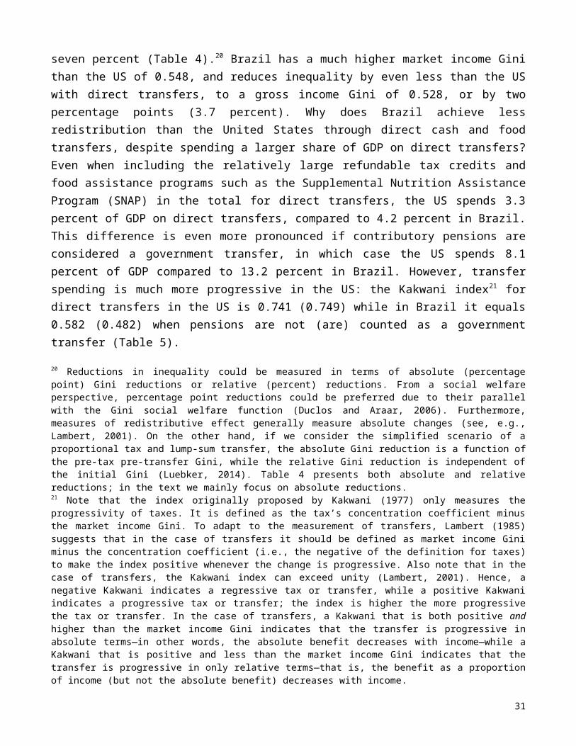
FIGURE 2. CONCENTRATION CURVES FOR TAX AND SPENDING CATEGORIES (BENCHMARK CASE), US 2011

Source: Authors’ calculations using Current Population Survey, American Community Survey, American Housing Survey, and National Household Education Survey.

In both countries, the poor pay a significant portion of their (market) income in indirect taxes:27 the poorest decile in Brazil pays 24 percent of its market income in indirect taxes and that of the US pays 16 percent. In March 2013, Brazil announced that it would end federal (but not state) taxes on a number of basic food items, which will likely mitigate this large effect on the poor. In contrast, in the United States, many states have been moving in the opposite direction by increasing their regressive sales taxes and, in some cases, decreasing income and property taxes.28 These sales taxes place a large burden on the poor, and not only financially: Newman and O’Brien (2011) exploit intra-state variation over time in the tax burden on the poor (in the US) and find that a higher tax burden on the poor has a statistically and economically significant impact on mortality, obesity, and violent crime.

27 Not disposable income, which is significantly higher for the poorest decile. Hence, they pay a lower percent of their disposable income in indirect taxes.

31

The high burden of indirect taxes on the poor in both countries can also be seen by the fact that, when all taxes are taken together (dotted dark gray curve in Figures 2 and 3), although the overall tax mix is summarized as progressive by the Kakwani index in both countries, it is not progressive across the entire distribution. The concentration curve for all taxes lies above the market income Lorenz curve at the lower end of the distribution—for at least the poorest 20 percent of the population in each country—indicating that these individuals pay a larger proportion of total taxes than their proportion of income. We verify the statistical significance of this result by testing a null hypothesis of non-dominance on these restricted domains, using the asymptotic sampling distributions for Lorenz and concentration curves derived by Davidson and Duclos (1997).

iv Indirect Subsidies

Subsidies are highly progressive in both the US and Brazil, as can be seen by the dotted light gray curves in Figures 1 and 2. These programs, which are among the best-targeted in each country, include energy subsidies for households who consume below a certain quantity of kilowatt-hours per month (and, in some cases, also have income below a certain threshold) and subsidized housing for low-income families. In the US, housing subsidies are more progressive and well-targeted than any other program, with a concentration coefficient of -0.858 (Table 6) and 94 percent of benefits going to the poorest 20 percent (bottom quintile) of the population. Household energy subsidies are also very progressive in the US, with a concentration coefficient of -0.720, making them the third most progressive program in the country behind heating subsidies and welfare benefits.29 They are also well-targeted, with 73 percent of benefits going to the bottom quintile.

In Brazil, the main housing subsidy program Minha Casa Minha Vida was not implemented until late 2009 (after the household survey had already taken place), so it is not included in our analysis. Targeted energy subsidies constitute the fourth-most progressive program in Brazil, behind its well-targeted cash transfer programs (Bolsa Família and BPC) and its milk transfer program. The program is less well-targeted than in the US, with 40 percent of benefits going to the poorest

28 Out of four sources of tax revenue—property tax, sales tax, individual income tax, and corporate income tax—the Midwest and West regions of the US have shifted from relying on property taxes more than any other tax in 1957 to relying on sales taxes more than any other in 2006 (Newman and O’Brien, 2011). Between 2007 and 2011, thirteen states and the District of Columbia increased state sales tax rates (Tax Foundation, 2012). A very recent example of a state that has simultaneously increased sales taxes and reduced income taxes is Ohio, whose tax reform went into effect on September 1, 2013. Globalization may provide additional pressure on states and the country as a whole to shift from individual and corporate income taxes to expenditure taxes (Hines and Summers, 2009). 29 “Welfare” includes a number of programs including longstanding welfare programs, as well as newer programs such as AFDC and TANF.

32

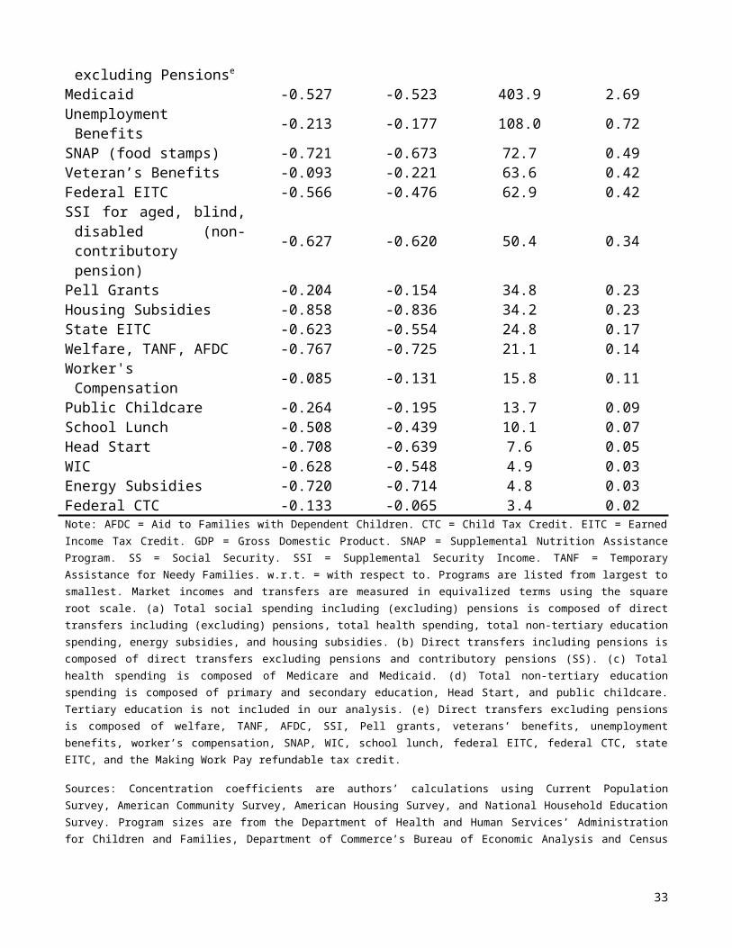
quintile of the population. In addition, the program is extremely small, at 0.05 percent of GDP, which limits its redistributive impact.

v Public Spending on Non-Tertiary Education and Health

As noted in Garfinkel et al. (2006, 2010), public spending on non-tertiary education and health is a particularly important part of redistribution in the US: when it is included in the analysis, the gap in terms of redistribution between the US and Europe is significantly reduced. In our analysis, this manifests itself in the fact that, when adding government spending on public childcare, the Head Start preschool program, primary and secondary education, and health spending on the poor and elderly through Medicaid and Medicare to incomes, the Gini is reduced by a further six percentage points, from a post-fiscal income Gini coefficient of 0.380 to a final income Gini of 0.319 in the benchmark case. No adjustment is made for quality of service; the public spending allocated to households is inflated by the fact that healthcare costs in the US are astronomically high, but health outcomes are no better than in European countries where healthcare is significantly less expensive (Anderson et al., 2003). Keeping this caveat in mind, social spending and taxation as a whole in the United States (excluding contributory pensions) results in a thirteen percentage point reduction in the Gini coefficient between market and final income, from 0.446 to 0.319. When pensions are considered a transfer and contributions treated as a tax, social spending and taxation as a whole reduces income inequality by seventeen percentage points, from 0.481 to 0.314.30

All components of education spending (public childcare, Head Start, and primary and secondary) are progressive in absolute terms, meaning that the poor benefit more than proportionally to their population size. This result is not always desirable, however; the absolute progressivity of primary and secondary education, for example, may be the result of rich families choosing to send their children to private schools due to quality concerns. In contrast, the high absolute progressivity of the Head Start program (with a concentration coefficient of -0.708) is due to the deliberate targeting by the government of a program with limited budget resources. Under the current (and tightening) budget constraints of the program, the high level of progressivity indicates that it is reaching the neediest families, for whom returns to investment in early childhood education are highest (Heckman, 2011) and whose children often otherwise reach kindergarten already possessing a large cognitive gap relative to their peers that persists throughout their education (Heckman, 2008).30 Comparisons with other developed countries are difficult because most studies do not include the benefits of public education and health spending in income despite the early efforts of Smeeding et al. (1993) to include them; Garfinkel et al. (2006, 2010) find that inequality in the US is considerably closer to inequality in other OECD countries after indirect taxes and health and education benefits are included.

33

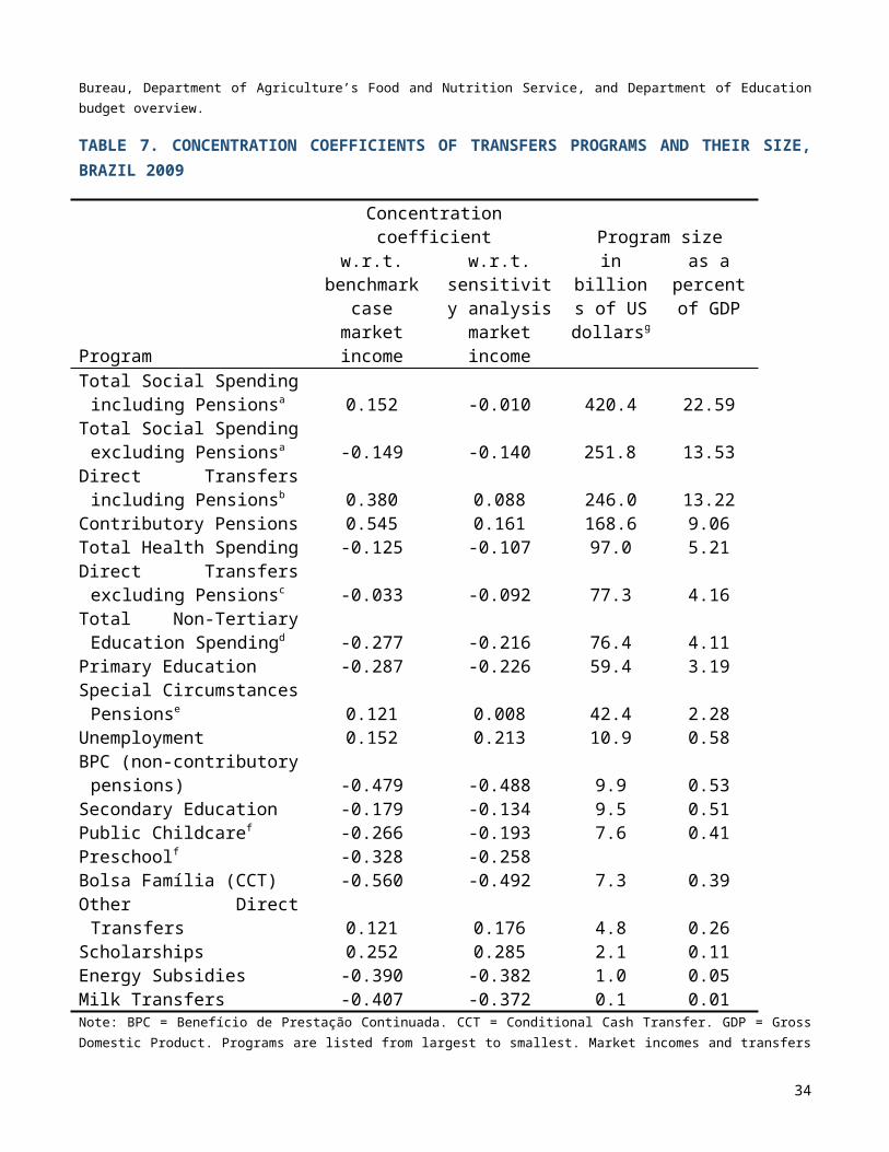
In Brazil, health and non-tertiary education spending has an even larger impact on income distribution: when adding government spending on non-tertiary education and health to income, the Gini coefficient is reduced by nearly eight additional percentage points, from a post-fiscal income Gini of 0.510 to a final income Gini of 0.431 (Table 1).31

Our analysis does not include tertiary education for comparability with the US, where data limitations prevented us from being able to identify the beneficiaries of public university spending. However, when the distribution of tertiary benefits are analyzed for Brazil, the results are abhorrent: tertiary education spending has a concentration coefficient of 0.470. This is fairly close to the Gini coefficient for income, indicating that the rich benefit about proportionally to their income from tertiary education. Furthermore, Higgins and Pereira (2014) find that, while 39 percent of the population aged 18-23 is poor,32 only 9 percent of 18-23 year olds who attend tertiary institutions belong to this group.

Overall, social spending and taxation (excluding pensions) reduce the Gini coefficient by slightly less in Brazil than in the US: Brazil reduces inequality by twelve percentage points (21 percent) compared to thirteen percentage points (29 percent) in the US. In contrast with the US, in Brazil the Gini reduction (from a market income Gini of 0.548 to a final income Gini of 0.431) was due mostly to public spending on education and health. When contributory pensions are treated as a government transfer and contributions as a tax, the Brazilian Gini is reduced from 0.570 to 0.428, or by fourteen percentage points (25 percent)—slightly less than the seventeen percentage point (35 percent) reduction in the US.

4 CONCLUSIONS

This paper presents the first direct comparison of fiscal incidence in Brazil and the United States, using household survey data and a combination of allocation techniques including direct identification, inference, simulation, prediction, and imputation. Such comparisons are indeed of interest because income inequality is high in both countries given their levels of development. Although Brazilian inequality is higher than in the US, its GDP per capita is much lower, at about one fourth of the US level. But inequality in America was at a similar level to inequality in Brazil today when it had a similar GDP per capita; for instance, 31 In comparison with market to final income redistribution in other developed countries, Brazil redistributes less overall than South Africa (which reduces inequality by 17.5 percentage points), about the same as Costa Rica (11.5 percentage points), and more than Armenia, Bolivia, El Salvador, Ethiopia, Guatemala, Indonesia, Jordan, Mexico, Peru, Sri Lanka, and Uruguay (see references in section 3.2).32 Poverty is defined as living in a household with household per capita income less than $4 PPP per day.

34

Plotnick et al. (1998) estimate the Gini for the US in monetary gross income terms to be around 0.55 in 1940, roughly the same level as in Brazil today. Furthermore, the levels of inequality in the two countries are getting closer, with inequality declining in Brazil over the last decade (Lustig et al., 2013b) and persistently rising in the US (Kenworthy and Smeeding, 2014).

The two nations also have other similarities which can be noted. They have low intergenerational mobility (Jäntti et al., 2006, Corak, 2013) and high equality of opportunity (Brunori et al., 2013). More obviously, they are both are relatively large, western hemisphere nations with substantial interregional inequality and large racial and ethnic minorities. The unequal distribution of human capital across races is an important determinant of income inequality in both countries (Card and Krueger, 1992, Ñopo, 2012).

So how well does each nation do in terms of reducing market income inequality, once we account for the incidence of almost all government social spending and taxes? The pre-fisc (market income) Gini in the United States is 0.446 and in Brazil it is 0.548. In the US it is reduced by 7.0 percentage points by direct transfers, indirect subsidies, and direct and indirect taxes, but by only 3.6 percentage points in Brazil. Neither nation is high on the list of OECD nations in inequality reduction through the fiscal system (Immervoll and Richardson, 2013, Joumard et al., 2012), which explains in part the high poverty rates in both countries (Morelli et al., forthcoming).

Public spending on health and education is larger than on cash and near cash transfers in both countries. When we add public spending on health and education to income, the decline in the Gini coefficients are almost identical in both countries. These results must be analyzed with some caveats in mind: specifically, that inequality reduction may be inflated if middle and upper class citizens opt out of the public education and health sectors, and that spending amounts do not reflect quality (which comes into play in both the US with respect to inflated health care costs and in Brazil with respect to low quality services).

In the United States, the market income Gini coefficient declines by 12.7 percentage points when direct cash and food transfers, housing and energy subsidies, individual and corporate income taxes, property taxes, expenditure taxes, and public spending on health (Medicare and Medicaid) and education (public primary and secondary school, Head Start, and public daycare through CCDF and TANF) are included in the income concept. When contributory pensions are counted as a government transfer, the Gini declines by 16.8 percentage points.

35

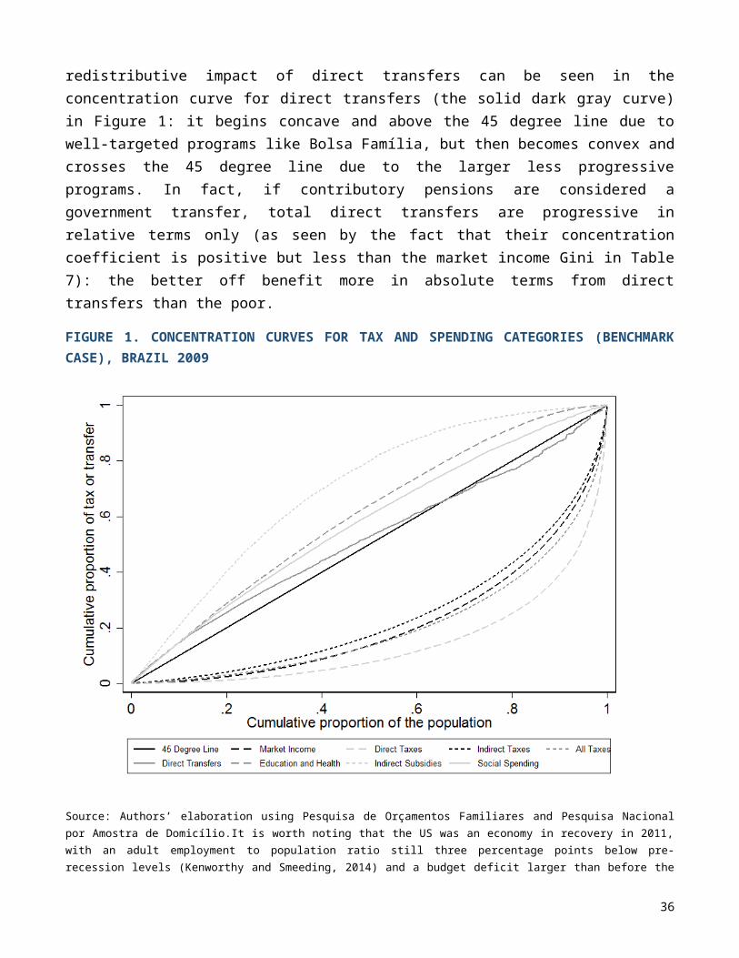
In Brazil, the Gini coefficient is reduced by 11.7 percentage points when we include all of these components in income, where health spending is in the form of free care received at public health facilities and education spending is in the form of public primary and secondary school, public pre-school, and free public daycare for low income families. When pensions are considered a transfer, the Gini declines by 14.2 percentage points. The conclusions from our comparison are robust to other adjustments for family size (Appendix A in the online supplement).

The lessons from this exercise are instructive. Transfers that maintain consumption are usually in cash or near cash terms. Transfers that can be seen as investments in human capital (health and education) are most often in-kind. In the United States the systems are separate, but generally targeted to the poor. In Brazil, the relatively massive Bolsa Família delivers both consumption (to families) and education and healthcare to their children, in a well-targeted program. Some have argued that the United States ought to consider a similar program; conditional cash transfer programs modeled after Bolsa Família and Mexico’s Oportunidades have in fact been piloted in New York City, Memphis, and the Bronx—their expansion at the national level could prove to be an important redistributive instrument.

Meanwhile, Brazil could benefit from higher quality schools and healthcare (though not at US prices). In addition, now that Brazil’s extreme poor are almost universally covered by at least one cash transfer program (Lustig et al., 2013a), the country might consider incentivizing formality through refundable tax credits. The EITC has been shown to increase labor force participation (Eissa and Liebman, 1996) and intergenerational mobility (Chetty et al., 2013), perhaps because recipients use a portion of the benefits for expenses that help improve economic and social mobility (Smeeding et al., 2000). It also improves infant health among beneficiary mothers, with a larger improvement for blacks (Hoynes et al., forthcoming). Brazil might also consider implementing a targeted large-scale food assistance program like SNAP, which is the United States’ most effective anti-poverty program for the non-elderly (Tiehan et al., 2013). Furthermore, both EITC and SNAP were exceptionally responsive to the recession (Immervoll and Richardson, 2013, Ziliak, 2013), and had an increasing impact on poverty reduction between 2011 and 2012 (Short, 2013).

Perhaps each country could benefit by mimicking the best aspects of the social spending and taxation systems in the other country. Nevertheless, we would rather suggest that both countries look at the way that other large nations such as Australia and Canada finance and deliver public services with better and more pro-poor redistribution and more equality, resulting in higher levels of intergenerational mobility (Ermisch et al., 2012).

36

37

REFERENCES

Aaberge, R., A. Björklund, M. Jäntti, M. Palme, P. J. Pedersen, N. Smith, and T. Wennemo, “Income Inequality and Income Mobility in the Scandinavian Countries Compared to the United States,” Review of Income and Wealth 48, 443–469, 2002.

Alm, J. and E.B. Sennoga, “Mobility, Competition, and the Distributional Effects of Tax Evasion,” National Tax Journal, 63 (4), 1055–1084, 2010.

Alm, J. and K. Finlay, “Who Benefits from Tax Evasion?” Economic Analysis and Policy, 43(2), 139–154, 2013.

Alm, J., R. Bahl, and M.N. Murray, “Tax Structure and Tax Compliance,” Review of Economics and Statistics, 72(4), 603–613, 1990.

Alvaredo, F. and L. Gasparini, “Recent Trends in Inequality and Poverty in Developing Countries,” in A.B. Atkinson and F. Bourguignon, eds., Handbook of Income Distribution, vol. 2, Elsevier, Amsterdam, forthcoming.

Anderson, G.F., U.E. Reinhardt, P.S. Hussey, and V. Petrosyan, “It’s the Prices, Stupid: Why the United States is so Different from Other Countries,” Health Affairs, 22, 89–105, 2003.

Atkinson, A.B. and S. Morelli, “Chartbook of Economic Inequality: 25 Countries,” Institute for New Economic Thinking Research Note 015, 2012.

Atkinson, A.B., L. Rainwater, and T.M. Smeeding, “Income Distribution in OECD Countries: Evidence from the Luxembourg Income Study (LIS),” Social Policy Studies No. 18, Organization for Economic Cooperation and Development, Paris, 1995.

Auerbach, A.J., “Who Bears the Corporate Tax? A Review of What We Know,” In J.M. Poterba, ed., Tax Policy and the Economy, volume 20, MIT Press, Cambridge, 2006.

Borjas, G.J., “The Wage Structure and the Sorting of Workers in the Public Sector,” Working Paper 9313, National Bureau of Economic Research, Cambridge, 2002.

Bosch, M. and R. Campos, “The Trade-offs of Social Assistance Programs in the Labor Market: the Case of the Seguro Popular Program in Mexico,” Centro de Estudios Económicos Working Paper 2010-12, Colegio de México, Mexico City, 2010.

Bourguignon, F., F.H.G. Ferreira, and M. Menéndez, “Inequality of Opportunity in Brazil,” Review of Income and Wealth, 53(4), 585–618, 2007.

38

Bourguignon, F., F.H.G. Ferreira, and P. G. Leite, “Beyond Oaxaca-Blinder: Accounting for Differences in Household Income Distributions,” Journal of Economic Inequality, 6, 117–148, 2008.

Bradbury, B., “The Fourth Retirement Pillar in Rich Countries,” in J. C. Gornick and M. Jäntti, eds., Income Inequality: Income Disparities and the Middle Class in Affluent Countries, Stanford University Press, California, 2013.

Braga, B., S. Firpo, and G. Gonzaga, “Escolaridade e o Diferencial de Rendimentos entre o Setor Privado e o Setor Público no Brasil,” Pesquisa e Planejamento Econômico, 39, 431–464, 2009.

Brandolini, A. and T.M. Smeeding, “Income Inequality in Richer and OECD Countries,” in W. Salverda, B. Nolan, and T.M. Smeeding, eds., Oxford Handbook of Economic Inequality, 71–100, Oxford University Press, Oxford, 2009.

Brunori, P., F.H.G. Ferreira, and V. Peragine, “Inequality of Opportunity, Income Inequality and Economic Mobility: Some International Comparisons,” Discussion Paper 7155, Institute or the Study of Labor (IZA), Bonn, 2013.

Bucheli, M., N. Lustig, M. Rossi, and F. Amábile, “Social Spending, Taxes and Income Redistribution in Uruguay,” Public Finance Review, 42, 413-433, 2014.

Buhmann, B., L. Rainwater, G. Schmauss, and T.M. Smeeding, “Equivalence Scales, Well-being, Inequality, and Poverty: Sensitivity Estimates Across Ten Countries using the Luxembourg Income Study Database,” Review of Income and Wealth, 34, 115–142, 1988.

Bureau of Economic Analysis, U.S. Economic Accounts, 2013 (http://www.bea.gov/).

Cabrera, M., N. Lustig, and H.E. Morán, “Fiscal Policy, Inequality and the Ethnic Divide in Guatemala,” CEQ Working Paper No. 20, 2014.

Callan, T., T.M. Smeeding, and P. Tsakloglou, “Short-Run Distributional Effects of Public Education Transfers to Tertiary Education Students in Seven European Countries,” Education Economics, 16(3), 275–288, 2008.

Camacho, A., E. Conover, and A. Hoyos, “Effects of Colombia’s Social Protection System on Workers’ Choice between Formal and Informal Employment,” Policy Research Working Paper 6564, World Bank, Washington, D.C., 2013.

Capeau, B., A. Decoster, and D. Phillips, “Consumption and Indirect Tax Microsimulation,” in C. O’Donoghue, ed., Handbook of Microsimulation Modelling, Emerald, forthcoming.

39

Card, D. and A.A. Payne, “School Finance Reform, the Distribution of School Spending, and the Distribution of Test Scores,” Journal of Public Economics, 83, 49-82, 2002.

Card, D. and A.B. Krueger, “School Quality and Black-White Relative Earnings: A Direct Assessment,” Quarterly Journal of Economics, 107, 151–200, 1992.

CEDLAS (Centro de Estudios Distributivos, Laborales y Sociales) and the World Bank, Socio-Economic Database for Latin America and the Caribbean, 2013 (http://sedlac.econo.unlp.edu.ar/).

Census Bureau, “Public Education Finances: 2010,” Governments Division Reports, US Census Bureau, Washington, D.C., 2012.

Chetty, R., N. Hendren, P. Kline, and E. Saez, “The Economic Impacts of Tax Expenditures: Evidence from Spatial Variation across the U.S.,” mimeo, 2013 (http://obs.rc.fas.harvard.edu/chetty/tax_expenditure_soi_whitepaper.pdf).

Congressional Budget Office, “The 2013 Long-Term Budget Outlook,” 2013 (http://www.cbo.gov/sites/default/files/cbofiles/attachments/44521-LTBO-1Column_0.pdf).

Corak, M., “Inequality from Generation to Generation: The United States in Comparison,” in R.S. Rycroft, ed., The Economics of Inequality, Poverty, and Discrimination in the 21st Century, Santa Barbara, ABC – CLIO, 2013.

Corbacho, A., V.F. Cibils, and E. Lora, More than Revenue: Taxation as a Development Tool, Palgrave Macmillan, New York, 2013.

Davidson, R. and J.-Y. Duclos, “Statistical Inference for the Measurement of the Incidence of Taxes and Transfers,” Econometrica, 65, 1453–1465, 1997.

Davis, C., K. Davis, M. Gardner, H. Heimovitz, R.S. McIntyre, R. Phillips, A. Sapozhnikova, M. Wiehe, Who Pays? A Distributional Analysis of the Tax Systems in All 50 States, 4th edition, Institute on Taxation and Economic Policy, Washington, D.C., 2013.

Deaton, A., “Counting the World’s Poor: Problems and Possible Solutions,” World Bank Research Observer, 16, 125–147, 2001.

Denk, O., R. Hagemann, P. Lenain, and V. Somma, “Inequality and Poverty in the United States: Public Policies for Inclusive Growth,” Economics Department Working Paper, Organisation for Economic Co-operation and Development (OECD), Paris, 2013.

Duclos, J.-Y., and A. Araar, Poverty and Equity: Measurement, Policy, and Estimation with DAD, Springer, New York, 2006.

40

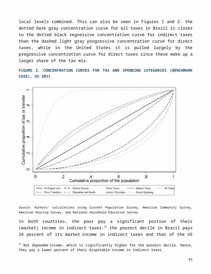
Eissa, N. and J.B. Liebman, “Labor Supply Response to the Earned Inccome Tax Credit,” Quarterly Journal of Economics, 112, 605–637, 1996.

Engel, E.M.R.A., A. Galetovic, and C.E. Raddatz, “Taxes and Income Redistribution in Chile: Some Unpleasant Redistributive Arithmetic,” Journal of Development Economics, 59, 155–192, 1999.

Ermisch, J., M. Jäntti, T. Smeeding, and J. Wilson, “Advantage in Comparative Perspective,” in J. Ermisch, M. Jäntti, and T. Smeeding, (eds.), From Parents to Children: The Intergenerational Transmission of Advantage, New York, Russell Sage Foundation, 3–31, 2012.

EUROMOD, “Effect of Tax-Benefit Components on Inequality,” EUROMOD Statistics, 2014 (https://www.iser.essex.ac.uk/files/euromod/Statistics/WebStatistics_July1_2014_Gini_Datasets_Population_Exchangerates.xlsx).

Ferraz, C., F. Finan, and D. B. Moreira, “Corrupting Learning: Evidence from Missing Federal Education Funds in Brazil,” Journal of Public Economics, 96, 712-726, 2012.

Ferreira, F.H.G., P.G. Leite, and J.A. Litchfield, “The Rise and Fall of Brazilian Inequality: 1981–2004,” Macroeconomic Dynamics, 12, 199—230, 2008.

Ferreira, F.H.G., J. Messina, J. Rigolini, L.F. López-Calva, M. Ana Lugo, and R. Vakis, Economic Mobility and the Rise of the Latin American Middle Class, World Bank, Washington, DC, 2013.

Fujiwara, T., “Voting Technology, Political Responsiveness, and Infant Health: Evidence from Brazil,” working paper, 2013.

Garber, A.M. and J. Skinner, “Is American Health Care Uniquely Inefficient?” Journal of Economic Perspectives, 22, 27-50, 2008.

Garfinkel, I., L. Rainwater, and T.M. Smeeding, Wealth and Welfare States: Is America a Laggard or Leader? Oxford, UK: Oxford University Press, 2010.

_____, “A Re-examination of Welfare States and Inequality in Rich Nations: How In-kind Transfers and Indirect Taxes Change the Story,” Journal of Policy Analysis and Management, 25(4), 897–919, 2006.

Garganta, S. and L. Gasparini, “El Impacto de un Programa Social Sobre la Informalidad Laboral: el Caso de la AUH de Argentina,” CEDLAS Working Paper 133, CEDLAS, La Plata, Argentina, 2012.

Goldin, C., and L. Katz, The Race Between Education and Technology, Harvard University Press, Cambridge, 2008.

41

Hall, R.E. and C.I. Jones, “The Value of Life and the Rise in Health Spending,” Quarterly Journal of Economics, 122, 39-72, 2007.

Heckman, J.J., “Schools, Skills, and Synapses,” Economic Inquiry, 46(3), 289–324, 2008.

_____, “Effective Child Development Strategies,” in Zigler, E., W.S. Gilliam, and W.S. Barnett, eds., The Pre-K Debates: Current Controversies and Issues, Paul H. Brookes Publishing Co., Baltimore, 2011.

Higgins, S. and C. Pereira, “The Effects of Brazil’s Taxation and Social Spending on the Distribution of Household Income,” Public Finance Review, 42, 346-367, 2014.

Hoynes, H., D. Miller, and D. Simon, “Income, The Earned Income Tax Credit, and Infant Health,” American Economic Journal: Economic Policy, forthcoming.

Hines, Jr., J.R., and L. Summers, “How Globalization Affects Tax Design,” in J.R. Brown and J.M. Poterba, eds., Tax Policy and the Economy, vol. 23, 123–157, University of Chicago Press, Chicago, 2009.

International Monetary Fund, “United States 2013 Article IV Consultation,” Country Report 13/236, International Monetary Fund, Washington, D.C., 2013 (http://www.imf.org/external/pubs/ft/scr/2013/cr13236.pdf).

Immervoll, H., H. Levy, J.R.B. Nogueira, C. O’ Donoghue, and R. Bezerra, “The Impact of Brazil’s Tax-benefit System on Inequality and Poverty,” in S. Klasen and F. Nowak-Lehmann, eds., Poverty, Inequality, and Policy in Latin America, MIT Press, Cambridge, 2009.

Immervoll, H. and L. Richardson, “Redistribution Policy in Europe and the United States: Is the Great Recession a ‘Game Changer’ for Working-age Families?” Social, Employment and Migration Working Papers No. 150, OECD Publishing, Paris, 2013

(http://dx.doi.org/10.1787/5k44xwtc0txp-en).

Jäntti, M., K. Røed, R. Naylor, A. Björklund, B. Bratsberg, O. Raaum, E. Österbacka, and T. Eriksson, “American Exceptionalism in a New Light: A Comparison of Intergenerational Earnings Mobility in the Nordic Countries, the United Kingdom, and the United States,” Discussion Paper 1938, Institute for the Study of Labor (IZA), Bonn, 2006.

Jaramillo, M., “The Incidene of Social Spending and Taxes in Peru,” Public Finance Review, 42, 291-412, 2014.

Johnson, D. and T. Smeeding, “Inequality Measurement,” in J. Wright, ed., International Encyclopedia of Social and Behavioral Sciences, 2nd edition, Elsevier Ltd., Oxford, forthcoming.

42

Joumard, I., M. Pisu and D. Bloch, “Tackling Income Inequality: The Role of Taxes and Transfers,” OECD Journal: Economic Studies, 2012, 37-70, 2012.

Kakwani, N.C., “Measurement of Tax Progressivity: an International Comparison,” The Economic Journal, 87, 71–80, 1977.

Kenworthy, L. and T. Smeeding, "The United States: High and Rapidly-Rising Inequality," in B. Nolan and W. Salverda, eds., Inequality and Its Impacts, volume 2, Oxford University Press, Oxford, 695-717, 2014.

Kim, K. and P.J. Lambert, “Redistributive Effect of U.S. Taxes and Public Transfers, 1994-2004,” Public Finance Review, 37, 3–26, 2009.

Lambert, P.J., The Distribution and Redistribution of Income, 3rd edition, Manchester University Press, Manchester, 2001.

_____, “On the Redistributive Effect of Taxes and Benefits,” Scottish Journal of Political Economy, 32, 39–54, 1985.

Levy, S. and N. Schady, “Latin America’s Social Policy Challenge: Education, Social Insurance, Redistribution,” Journal of Economic Perspectives, 27, 193–218, 2013.

Litschig, S. and K.M. Morrison, “The Impact of Intergovernmental Transfers on Education Outcomes and Poverty Reduction,” American Economic Journal: Applied Economics, 5, 206–240, 2013.

Lora, E. and J. Fajardo, “Employment and Taxes in Latin America: an Empirical Study of the Effects of Payroll, Corporate Income and Value-added Taxes on Labor Outcomes,” Working Paper IDB-WP-334, Inter-American Development Bank, Washington, D.C., 2012a.

_____, “¿Hay un Sesgo Anti-laboral en los Impuestos en América Latina?”, Resumen de Políticas IDB-PB-177, Inter-American Development Bank, Washington, D.C., 2012b.

Luebker, M., “Income Inequality, Redistribution, and Poverty: Contrasting Rational Choice and Behavioral Perspectives,” Review of Income and Wealth, 60, 133-154, 2014.

Lustig, N., “Taxes, Transfers, Inequality and the Poor in the Developing World,” CEQ Working Paper No. 23, 2014.

_____ and S. Higgins, “Commitment to Equity (CEQ): Estimating the Incidence of Social Spending, Subsidies, and Taxes Handbook,” CEQ Working Paper No. 1, 2013 (http://www.commitmentoequity.org/publications_files/Methodology/CEQWPNo1%20Handbook%20Edition%20Sept%202013.pdf).

43

_____, C. Pessino, and J. Scott, “The Impact of Taxes and Social Spending on Inequality and Poverty in Argentina, Bolivia, Brazil, Mexico, Peru and Uruguay,” Public Finance Review, 42, 287-303, 2014.

_____, F. Amábile, M. Bucheli, G. Gray Molina, S. Higgins, M. Jaramillo, W. Jiménez Pozo, V. Paz Arauco, C. Pereira, M. Rossi, J. Scott, and E. Yáñez Aguilar, “The Impact of Taxes and Social Spending on Inequality and Poverty in Argentina, Bolivia, Brazil, Mexico, Peru and Uruguay: an Overview,” CEQ Working Paper No. 13, 2013a.

_____, L.F. López-Calva, and E. Ortiz-Juárez, “Declining inequlaity in Latin America in the 2000s: The cases of Argentina, Brazil, and Mexico,” World Development, 44(1): 129–141, 2013b.

Medeiros, M. and P.H.G.F. Souza, “The State and Income Inequality in Brazil,” Institute for Research on Labor and Employment Working Paper, University of California at Berkeley, Berkeley, 2013.

Milanovic, B., “Determinants of Cross-Country Income Inequality: An ‘Augmented’ Kuznets’ Hypothesis,” Policy Research Working Paper 1246, World Bank, Washington, D.C., 1994.

Ministério da Fazenda, Balanço do Setor Público Nacional: Exercício de 2009, 2010 (http://www3.tesouro.gov.br/contabilidade_governamental/downloads/Balanco_Setor_publico_Nacional.pdf).

Morelli, S., J. Thompson, and T.M. Smeeding, “Post-1970 Trends in Within-Country Inequality and Poverty,” in A. Atkinson and F. Bourguignon, eds., Handbook of Income Distribution, vol. 2, forthcoming.

Newman, K. and R. O’Brien, Taxing the Poor: Doing Damage to the Truly Disadvantaged, University of California Press, Berkeley, 2011.

Nogueira, J.R.B., R. Bezerra, and E.S. de Souza, “A Brazilian Tax-benefit Microsimulation Model,” in C.M. Urzúa, ed., Microsimulation Models for Latin America, 19–50, International Development Research Center and United Nations Development Programme and Tecnológico de Monterrey, Mexico City, 2011.

Ñopo, Hugo, New Century, Old Disparities: Gender and Ethnic Earnings Gaps in Latin America and the Caribbean, Inter-American Development Bank and World Bank, Washington, D.C., 2012.

OECD (Organisation for Economic Co-operation and Development), Society at a Glance 2014 OECD Social Indicators: The Crisis and its Aftermath, OECD Publishing, Paris, 2014.

44

_____, Divided We Stand: Why Inequality Keeps Rising, OECD Publishing, Paris, 2011a.

_____, Strong Performers and Successful Reformers in Education: Lessons from PISA for the United States, OECD Publishing, Paris, 2011b.

_____, “PISA 2009 Results: Executive Summary,” OECD Publishing, Paris, 2010.

Paz Arauco, V., G. Gray Molina, E. Yáñez Aguilar, W. Jiménez Pozo, “Explaining Low Redistributive Impact in Bolivia,” Public Finance Review, 42, 326-345, 2014.

Plotnick, R., E. Smolensky, E. Evenhouse and S. Reilly, “Inequality, Poverty, and the Fisc in Twentieth-century America,” Journal of Post Keynesian Economics, 21, 51–75, 1998.

Poterba, J.M., “Lifetime Incidence and the Distributional Burden of Excise Taxes,” American Economic Review Papers and Proceedings 79, 325–330, 1989.

Poterba, J.M. and K.S. Rueben, “The Distribution of Public Sector Wage Premia: New Evidence using Quantile Regression Methods,” Working Paper 4734, National Bureau of Economic Research, Cambridge, 1994.

Sauma, P. and J.D, “Gasto Público Social, Impuestos, Redistribución del Ingreso y Pobreza en Costa Rica,” CEQ Working Paper No. 18, 2014.

Scott, J., “Redistributive Impact and Efficiency of Mexico’s Fiscal System,” Public Finance Review, 42, 368-390, 2014.

Short, K., The Research Supplemental Poverty Measure: 2012, U.S. Census Bureau, Washington, D.C., 2013 (http://www.census.gov/prod/2013pubs/p60-247.pdf).

_____ and A. O’Hara, “Valuing Housing in Measures of Household and Family Economic Well-Being,” prepared for the Annual Meeting of the Allied Social Sciences Associations, 2008 (http://www.census.gov/housing/ahs/files/valuing_housing.pdf).

Smeeding, T.M., “Public Policy, Economic Inequality, and Poverty: The United States in Comparative Perspective,” Social Science Quarterly, 86, 955-983, 2005.

_____, K.R. Phillips, and M. O’Conner, “The EITC: Expectation, Knowledge, Use, and Economic and Social Mobility,” National Tax Journal, 53, 1187–1210, 2000.

_____, P. Saunders, J. Coder, S. Jenkins, J. Fritzell, A.J.M. Hagenaars, R. Hauser, and M. Wolfson, “Poverty, Inequality, and Family Living Standards Impacts across Seven Nationas: The Effect of Noncash Subsidies for Health, Educaiton and Housing,” Review of Income and Wealth, 39, 229-256, 1993.

45

Soares, F.V., S. Soares, M. Medeiros, and R.G. Osório, “Programas de Transferência de Renda no Brasil: Impactos sobre a Desigualdade,” in R. Paes de Barros, M.N. Foguel, and G. Ulyssea, eds., Desigualdade de Renda no Brasil: uma Análise da Queda Recente, volume 2, 87–129, Instituto de Pesquisa Econômica Aplicada, Brasilia, 2007.

Souza, P.H.G.F. and M. Medeiros, “The Decline in Inequality in Brazil, 2003-2009: the Role of the State,” Institute for Research on Labor and Employment Working Paper, University of California at Berkeley, Berkeley, 2013.

Tax Foundation, “Trend #4: Sales Tax Increases,” Tax Foundation Fiscal Fact No. 310, 2012 (http://taxfoundation.org/article/trend-4-sales-tax-increases).

Tiehen, L., D. Jolliffe, and T. Smeeding. “The Effect of SNAP on Poverty,” presented at the Association for Policy Analysis and Management Annual Research Conference, 2013 (https://appam.confex.com/data/extendedabstract/appam/2013/Paper_7629_extendedabstract_457_0.pdf).

US Census Bureau, “Historical National Population Estimates: July 1, 1900 to July 1, 1999,” 2000 (http://www.census.gov/popest/data/national/totals/pre-1980/tables/popclockest.txt).

USDA (US Department of Agriculture), “Food Expenditures,” 2014 (http://www.ers.usda.gov/data-products/food-expenditures.aspx#.VCNp-fl5NAG).

Wallace, S., M. Wasylenko, and D. Weiner, “The distributional implications of the 1986 tax reform,” National Tax Journal, 44, 181–198, 1991.

Wilson, K., K. Lambright, and T. M. Smeeding, “School Finance, Equivalent Educational Expenditure and Income Distribution: Equal Dollars or Equal Chances for Success?” Education Finance and Policy, 1, 396–424, 2006.

World Bank, World DataBank, 2013 (http://databank.worldbank.org/data/home.aspx).

Ziliak, J.P., “Why Are So Many Americans on Food Stamps? The Role of the Economy, Policy, and Demographics,” presented at the Association for Public Policy Analysis and Management Annual Research Conference, 2013 (http://gatton.uky.edu/Faculty/Ziliak/Ziliak_SNAP_100413.pdf).

46

CEQ WORKING PAPER SERIESWORKING PAPER NO. 1Lustig, Nora and Sean Higgins. 2013. Commitment to Equity Assessment

(CEQ):   Estimating the Incidence of Social Spending, Subsidies and Taxes.   Handbook . CEQ Working Paper No. 1, Center for Inter-American Policy and Research and Department of Economics, Tulane University and Inter-American Dialogue, September.

WORKING PAPER NO. 2Lustig, Nora. 2013. Commitment to Equity: Diagnostic Questionnaire. CEQ

Working Paper No. 2, Center for Inter-American Policy and Research and Department of Economics, Tulane University and Inter-American Dialogue, January.

WORKING PAPER NO. 3Lustig, Nora and George Gray Molina, Sean Higgins, Miguel Jaramillo, Wilson

Jiménez, Veronica Paz, Claudiney Pereira, Carola Pessino, John Scott, and Ernesto Yañez. 2012. The Impact of Taxes and Social Spending on Inequality and Poverty in Argentina, Bolivia,Brazil, Mexico and Peru: A Synthesis of Results. CEQ Working Paper No. 3, Center for Inter-American Policy and Research and Department of Economics, Tulane University and Inter-American Dialogue, August.

WORKING PAPER NO. 4Lustig, Nora and Sean Higgins. 2013. Fiscal Incidence, Fiscal Mobility and the

Poor: A New Approach. CEQ Working Paper No. 4, Center for Inter-American Policy and Research and Department of Economics, Tulane University and Inter-American Dialogue, January.

WORKING PAPER NO. 5Lustig, Nora and Carola Pessino. 2013. Social Spending and Income

Redistribution in Argentina in the 2000s: the Rising Role of Noncontributory Pensions. CEQ Working Paper No. 5, Center for Inter-American Policy and Research and Department of Economics, Tulane University and Inter-American Dialogue, REVISED August 2013.

WORKING PAPER NO. 6Paz Arauco, Verónica, George Gray Molina, Wilson Jiménez Pozo, and Ernesto

Yáñez Aguilar. 2013. Explaining Low Redistributive Impact in Bolivia. CEQ Working Paper No. 6, Center for Inter-American Policy and Research and Department of Economics, Tulane University and Inter-American Dialogue, REVISED April.

WORKING PAPER NO. 7

Higgins, Sean and Claudiney Pereira. 2013. The Effects of Brazil’s High Taxation and Social Spending on the Distribution of Household Income. CEQ Working Paper No. 7, Center for Inter-American Policy and Research and Department of Economics, Tulane University and Inter-American Dialogue, REVISED May 2013.

WORKING PAPER NO. 8Scott, John. 2013. Redistributive Impact and Efficiency of Mexico’s Fiscal System.

CEQ Working Paper No. 8, Center for Inter-American Policy and Research and Department of Economics, Tulane University and Inter-American Dialogue, REVISED July 2013.

WORKING PAPER NO. 9Jaramillo Baanante, Miguel. 2013. The Incidence of Social Spending and Taxes in

Peru. CEQ Working Paper No. 9, Center for Inter-American Policy and Research and Department of Economics, Tulane University and Inter-American Dialogue, REVISED May 2013.

WORKING PAPER NO. 10Bucheli, Marisa and Nora Lustig, Máximo Rossi and Florencia Amábile. 2013.

Social Spending, Taxes, and Income Redistribution in Uruguay. CEQ Working Paper No. 10, Center for Inter-American Policy and Research and Department of Economics, Tulane University and Inter-American Dialogue, REVISED July 2013.

WORKING PAPER NO. 11Higgins, Sean and Nora Lustig, Julio Ramirez and Billy Swanson. 2013. Social

Spending, Taxes and Income Redistribution in Paraguay. CEQ Working Paper No. 11, Center for Inter-American Policy and Research and Department of Economics, Tulane University and Inter-American Dialogue, November.

WORKING PAPER NO. 12Alvaredo, Facundo and Juliana Londoño Vélez. 2013. High Incomes and Personal

Taxation in a Developing Economy: Colombia 1993-2010. CEQ Working Paper No. 12, Center for Inter-American Policy and Research and Department of Economics, Tulane University and Inter-American Dialogue, March.

WORKING PAPER NO. 13Lustig, Nora, and Carola Pessino and John Scott. 2013. The Impact of Taxes and

Social Spending on Inequality and Poverty in Argentina, Bolivia, Brazil, Mexico, Peru and Uruguay: An Overview. CEQ Working Paper No. 13, Center for Inter-American Policy and Research and Department of Economics, Tulane University and Inter-American Dialogue, REVISED August 2013.

WORKING PAPER NO. 14Higgins, Sean and Nora Lustig. 2013. Measuring Impoverishment: An Overlooked

Dimension of Fiscal Incidence . CEQ Working Paper No. 14, Center for Inter-American Policy and Research and Department of Economics, Tulane University and Inter-American Dialogue, April.

WORKING PAPER NO. 15Tanzi, Vito. 2013. Tax Reform in Latin America: A long term assessment . CEQ

Working Paper No. 15, Center for Inter-American Policy and Research and

Department of Economics, Tulane University and Inter-American Dialogue, April.

WORKING PAPER NO. 16Higgins, Sean, Nora Lustig, Whitney Ruble and Tim Smeeding. 2013. Comparing

the Incidence of Taxes and Social Spending in Brazil and the United States. CEQ Working Paper No. 16, Center for Inter-American Policy and Research and Department of Economics, Tulane University and Inter-American Dialogue, REVISED October 2014.

WORKING PAPER NO. 17López-Calva, Luis F., Nora Lustig, John Scott y Andrés Castañeda. 2014. Gasto

social, redistribución del ingreso y reducción de la pobreza en México: evolución y comparación con Argentina, Brasil y Uruguay. CEQ Working Paper No. 17, Center for Inter-American Policy and Research and Department of Economics, Tulane University and Inter-American Dialogue, REVISED March.

WORKING PAPER NO. 18 SpanishSauma, Juan Diego Trejos. 2014. Gasto público social, impuestos, redistribución

del ingreso y pobreza en Costa Rica. CEQ Working Paper No. 18, Center for Inter-American Policy and Research and Department of Economics, Tulane University and Inter-American Dialogue, January.

WORKING PAPER NO. 18 EnglishSauma, Juan Diego Trejos. 2014. Social Public Spending, Taxes, Redistribution of

Income, and Poverty in Costa. CEQ Working Paper No. 18, Center for Inter-American Policy and Research and Department of Economics, Tulane University and Inter-American Dialogue, January.

WORKING PAPER NO. 19Amábile, Florencia, Marisa Bucheli and Máximo Rossi. 2014. Inequality and

Poverty in Uruguay by Race: The Impact of Fiscal Policies. CEQ Working Paper No. 19, Center for Inter-American Policy and Research and Department of Economics, Tulane University and Inter-American Dialogue, February.

WORKING PAPER NO. 20Cabrera, Maynor, Nora Lustig and Hilcías Morán. 2014. Fiscal Policy, Inequality

and the Ethnic Divide in Guatemala. CEQ Working Paper No. 20, Center for Inter-American Policy and Research and Department of Economics, Tulane University and Inter-American Dialogue. October.

WORKING PAPER NO. 21Burdín, Gabriel, Fernando Esponda, and Andrea Vigorito. 2014. Inequality and

top incomes in Uruguay: a comparison between household surveys and income tax micro-data. CEQ Working Paper No. 21, Center for Inter-American Policy and Research and Department of Economics, Tulane University and Inter-American Dialogue, May.

WORKING PAPER NO. 22Lustig, Nora. 2014. Fiscal policy and ethno-racial inequality in Bolivia, Brazil,

Guatemala and Uruguay. CEQ Working Paper No. 22, Center for Inter-American Policy and Research and Department of Economics, Tulane University and Inter-American Dialogue. Forthcoming.

WORKING PAPER NO. 23Lustig, Nora. 2014. Taxes, Transfers, Inequality and the Poor in the Developing

World. Round 1. CEQ Working Paper No. 23, Center for Inter-American Policy and Research and Department of Economics, Tulane University and Inter-American Dialogue. Forthcoming.

WORKING PAPER NO. 24Lustig, Nora and Marcela Melendez. 2014. The Impact of Taxes and Transfers on

Inequality and Poverty in Colombia. CEQ Working Paper No 24, Center for Inter-American Policy and Research and Department of Economics, Tulane University and Inter-American Dialogue. Forthcoming.

WORKING PAPER NO. 25Lustig Nora, Rodrigo Aranda and Ali Enami. 2014. Measuring the Contribution of

Taxes and Transfers to Changes in Inequality and Poverty: How to Address Path Dependency. CEQ Working Paper No. 25, Center for Inter-American Policy and Research and Department of Economics, Tulane University and Inter-American Dialogue. Forthcoming.

WORKING PAPER NO. 26Beneke, Margarita, Nora Lustig y José Andrés Oliva. 2014. El impacto de los

impuestos y el gasto social en la desigualdad y la pobreza en El Salvador. CEQ Working Paper No. 26, Center for Inter-American Policy and Research and Department of Economics, Tulane University and Inter-American Dialogue. Forthcoming.

http://www.commitmentoequity.org