video analysis of head kinematics in boxing matches using opencv library under macintosh platform
TRANSCRIPT
IT 12 046
Examensarbete 30 hpSeptember 2012
Video analysis of head kinematics in boxing matches using OpenCV library under Macintosh platform How can the Posit algorithm be used in head
kinematic analysis?
Liyi Zhao
Institutionen för informationsteknologiDepartment of Information Technology


Teknisk- naturvetenskaplig fakultet UTH-enheten Besöksadress: Ångströmlaboratoriet Lägerhyddsvägen 1 Hus 4, Plan 0 Postadress: Box 536 751 21 Uppsala Telefon: 018 – 471 30 03 Telefax: 018 – 471 30 00 Hemsida: http://www.teknat.uu.se/student
Abstract
Video analysis of head kinematics in boxing matchesusing OpenCV library under Macintosh platform
Liyi Zhao
The division of Neuronic Engineering at KTH focuses the research on the head and neck biomechanics. Finite Element (FE) models of the human neck and head have been developed to study the neck and head kinematics as well as injurious loadings of various kinds. The overall objective is to improve the injury prediction through accident reconstruction.
This project aims at providing an image analysis tool which helps analyzers building models of the head motion, making good estimation of head movements, rotation speed and velocity during head collision. The applicability of this tool is a predefined set of boxing match videos. The methodology however, can be extended for the analysis of different kinds of moving head objects. The user of the analysis tool should have basic ideas of how the different functionalities of the tool work and how to handle it properly.
This project is a computer programming work which involves the study of the background, the study of methodology and a programming phase which gives result of the study.
Tryckt av: Reprocentralen ITCIT 12 046Examinator: Lisa KaatiÄmnesgranskare: Svein KleivenHandledare: Svein Kleiven

Contents
1 Introduction 11.1 Background and motivation 11.2 The research questions 11.3 Previous studies 21.4 Methodology 51.5 Structure of thesis 7
2 VirtualDub video capture and OpenCV image preprocessing 82.1 Objective 82.2 Video information extraction 92.3 Video deinterlacing, boosting and image sequence export using VirtualDub 102.4 Image preprocessing using OpenCV 13
3 Head kinematic analysis with head pose estimation using Posit algorithm 173.1 Head pose estimation and head kinematics 173.2 Head pose estimation and the Posit algorithm 193.3 Model simplification criterion and model division 243.4 The persistence of head model 263.5 Fast pose estimation using ear models 27
4 Posit head pose estimation in MotionTracker 294.1 Objective 294.2 The loading of inputs of Posit algorithm with drag-and-drop operation 294.3 The image point visual editing and the template method 314.4 Euler angle representation and its transformation into rotation velocity 344.5 Translation representation and its transformation into translation velocity 36
5 Head rotation estimation and evaluation 385.1 Representation of head rotation and translation speed 385.2 The interpolation of the velocity data 445.3 Accuracy from real pose: An evaluation 495.4 Summary of requirements and applicability of the method 54
6 Delimitation and conclusion 576.1 Delimitation 576.2 Summary and future studies 58
Appendix I : OpenCV focal length prediction using Posit algorithm hints 61
Appendix II : The creation of the simplified head model using MotionTracker 64
Appendix III : MotionTracker User Manual 66
References 72

FiguresFiguresFigures
Figure 1 Example of boxing match image sequence 2
Figure 2 The calibration rig(left) and human joints should be created and assigned for Skillspector motion analysis
3
Figure 3 Result of Skillspector shows the 3D head acceleration with respect to time in radians per second
3
Figure 4 Head pose can be estimated using only seven image points using solvePnP function 4
Figure 5 Given a image in the left, a template image in the middle, the template method could be used to find the pattern in the image that is closest to the template image used
5
Figure 6 Image deinterlacing should be used to improve the image quality of the TV images 5
Figure 7 Example of a sequence of head concussion images in a boxing match footage 9
Figure 8 AVI files taken from PAL or NTFS camcorder which shows interlaced pattern at odd and even lines
11
Figure 9 VirtualDub software, the window shows the first field of the video 12
Figure 10 Deinterlace-Smooth filter control panel which is used to fine control the video deinterlace process
12
Figure 11 HSV filter in VirtualDub can be used to boost the saturation of the image sequences 13
Figure 12 Image before and after deinterlacing and color boosting operation 13
Figure 13 Interface of MotionTracker tool 15
Figure 14 Example of the 3D model of the head. The points on the head lives in the space the we call the object coordinate system
17
Figure 15 Camera space is a typical selection of RCS 18
Figure 16 Mapping between the model points in OCS on the left and image points in RCS on the right
18
Figure 17 Rotation matrix and translation matrix transform the OCS 19
Figure 18 Yaw, Pitch and Row in the form of head rotation 22
Figure 19 Saving of head model into property list files using Xcode 27
Figure 20 Drag and Drop operation enables fast loading of image sequence and model files into Mo-tionTracker
30
Figure 21 Image points are saved alone with the image sequence 31
Figure 22 Image screen in MotionTracker demonstrates an image in the image sequence of the video
31
Figure 23 Image slider in MotionTracker 32
Figure 24 Mouse cursor represents where the image point is going to be selected 32

Figure 25 The process of the selection of the image point using the Right ear model 32
Figure 26 Automatic image point searching option in MotionTracker with the usage of template method
33
Figure 27 The process of editing image points in MotionTracker 34
Figure 28 Example of output of head pose values in MotionTracker 34
Figure 29 Representation of roll and yaw values in 2D cartesian space in MotionTracker 35
Figure 30 Representation of pitch values in 2D cartesian space in MotionTracker 35
Figure 31 Example output of head distance values in MotionTracker 36
Figure 32 Interpolated head velocity alone three axis in video 1 47
Figure 33 Rotation of the yaw value from 45 degree to 345 degree 58
Figure 34 Front View of the sample person is selected with the image points that is used to construct the head model
64
Figure 35 Side View of the sample person is selected with the image points that is used to construct the head model
65
TablesTablesTables
Table 1 Listing of boxing match movies to be analyzed 10
Table 2 Functionality implemented in MotionTracker 16
Table 3 Model Point Dictionary 20
Table 4 Image Point Dictionary 20
Table 5 Rotation and translation from OCS to CCS 21
Table 6 Assigned model object and image object for every image in the image sequence 24
Table 7 The procedure of the Posit algorithm 24
Table 8 Simplified head model of the sample person 25
Table 9 The left ear and the right ear model used in MotionTracker 26
Table 10 The left ear and the right ear model plotted in Matlab 26
Table 11 The way the template image is compared to the sliding window in the template method 33
Table 12 Head Rotation and Translation velocity in analyzed video using focal length equals to 1600
43
Table 13 Example output of head distance value 43
Table 14 Peak values during impact of analyzed video 48
Table 15 Peak value of L2 norm of the velocity during impact of analyzed video in radian per sec-ond
49
Table 16 Error of the head pose values 53
Table 17 Error of Tz with different input of focal length 62
Table 18 x and y component of the left ear model 65
Table 19 z component of the left ear model 65

This paper is based on [7]:
Enrico Pellegrini, Kinematic evaluation of traumatic brain injuries in boxing, 2011

1 Introduction
1.1 Background and motivation
Head injury of different kinds is one of the main causes of disabilities and deaths in the world. Traumatic brain injury, referred to as TBI, is one category of head injuries which occurs when the external forces traumatically injures the brain.
The report from World Health Organization (WHO) estimates that 2.78% of all deaths in the coun-tries within WHO region are related to the car incidents and unintentional falling[1]. High portion of these death numbers are related to TBI. WHO has also projected that, by 2020, traffic accidents will be the third greatest cause of the global burden of disease and injury[2]. It can be estimated that a lot of them would be TBI cases. Furthermore, TBI is also the most common cause of disability and death for young people in the USA in 2001[3][5].
According to a report from the department of defense in the USA, TBI can be divided into three main categories in terms of severity: mild TBI, moderate TBI and severe TBI. The severity can also be measured in the level of Glasgow coma scale, post-traumatic amnesia and loss of conscious-ness[4].
TBI can also be classified in terms of the mechanism that caused it, namely the closed TBI and the penetrating TBI. In the sport matches, most TBI injuries are closed cerebral injuries that is caused in the form of direct impact on the head. Prove has been shown that the type, direction, intensity, and duration of forces all contribute to the characteristics and severity of TBI[1].
To reduce the possibility of injuries and find new head protective measures, the mechanics of the impacts during the concussion is therefore very worth studying.
In this report, a research is carried out by the attempt to capture the head kinematic information through the analysis of a set of sports match videos from television which contains severe or mild level head concussions.
The main objective of this project is to find the head kinematic dynamics in the image sequence of the sports video. A computer software used for this purpose is designed and implemented. The func-tionality of this software includes: capture of the video footages, creation of head model points, im-provement of video images, and focal length estimation.
The result of the project, or the output of the software is a representation of the head kinematics in the analyzed video taking advantage of the knowledge from the computer vision library.
The motion analysis tool is developed under Mac OS X using Xcode.
The main library used for the motion analysis is OpenCV.
1.2 The research questions
The incentive of the project can be demonstrated by asking the research questions we are facing in the project.
Q: Given a sports video, what is the intended video format for the motion analysis or image proc-essing?
1
It is very important to get the right material for research. Given a motion video of the head object, it is not convenient or possible to make head kinematic analysis directly on video. A platform for cap-turing the image sequence from the video should be implemented.
Q: Given an image sequence, does the quality of the images satisfiable? How should we improve the quality of the images?
Ordinary TV footages usually have lower resolution compared to high definition videos. The inter-laced pattern is a another major flaw of quality in TV images. The quality of the videos should be improved in some way. For example, the level of noise should be reduced and the interlaced pattern should be deinterlaced.
Q: Where the image is loaded for analysis? Should there a platform for the motion analysis?
A tool or platform must be constructed for motion analysis of the head kinematics. The loading of image sequences, traverse of image sequences should also be implemented.
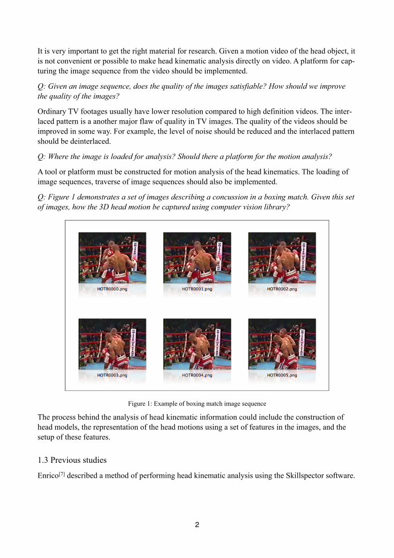
Q: Figure 1 demonstrates a set of images describing a concussion in a boxing match. Given this set of images, how the 3D head motion be captured using computer vision library?
Figure 1: Example of boxing match image sequence
The process behind the analysis of head kinematic information could include the construction of head models, the representation of the head motions using a set of features in the images, and the setup of these features.
1.3 Previous studies
Enrico[7] described a method of performing head kinematic analysis using the Skillspector software.
2
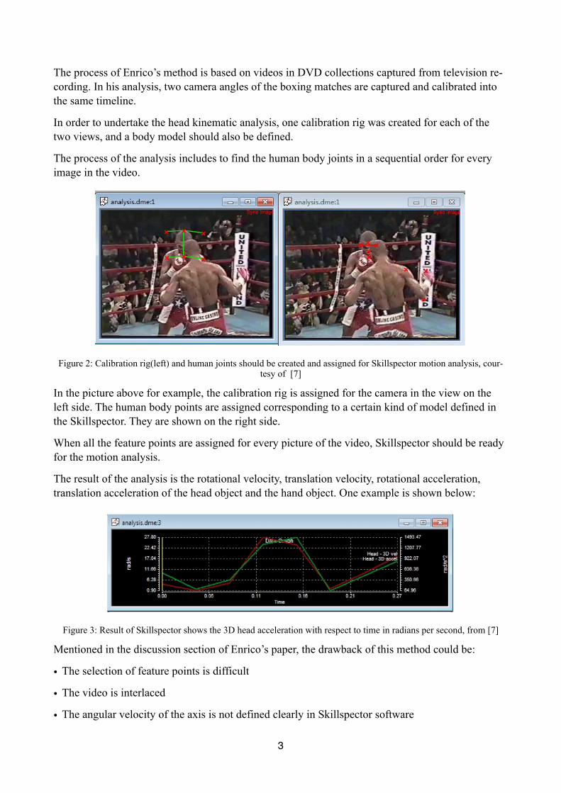
The process of Enrico’s method is based on videos in DVD collections captured from television re-cording. In his analysis, two camera angles of the boxing matches are captured and calibrated into the same timeline.
In order to undertake the head kinematic analysis, one calibration rig was created for each of the two views, and a body model should also be defined.
The process of the analysis includes to find the human body joints in a sequential order for every image in the video.
Figure 2: Calibration rig(left) and human joints should be created and assigned for Skillspector motion analysis, cour-tesy of [7]
In the picture above for example, the calibration rig is assigned for the camera in the view on the left side. The human body points are assigned corresponding to a certain kind of model defined in the Skillspector. They are shown on the right side.
When all the feature points are assigned for every picture of the video, Skillspector should be ready for the motion analysis.
The result of the analysis is the rotational velocity, translation velocity, rotational acceleration, translation acceleration of the head object and the hand object. One example is shown below:
Figure 3: Result of Skillspector shows the 3D head acceleration with respect to time in radians per second, from [7]
Mentioned in the discussion section of Enrico’s paper, the drawback of this method could be:
• The selection of feature points is difficult
• The video is interlaced
• The angular velocity of the axis is not defined clearly in Skillspector software
3
• Lack of evaluation method
In this paper, we are trying to overcome the disadvantage of the method in the Enrico’s paper and also taking advantage of the captured and calibrated videos from Enrico’s work.
Daniel[8]described an algorithm where the head kinematic information such as the orientation and position can be extracted using similar pattern as Enrico’s method. Daniel named this algorithm the Posit algorithm.
The similar pattern means, the kinematic information of the head object can be obtained by finding the correspondence between the image points and the model points of the object. This conception is firstly described and coined by Fischler[9] with the term Perspective-n-Point problem (PnP prob-lem).
There are also technical report[11] which inspires the way how we are going to refine the model in the Posit algorithm. The head model could be simplified into 4 points which makes Posit an intui-tive and feasible method for head kinematic analysis.
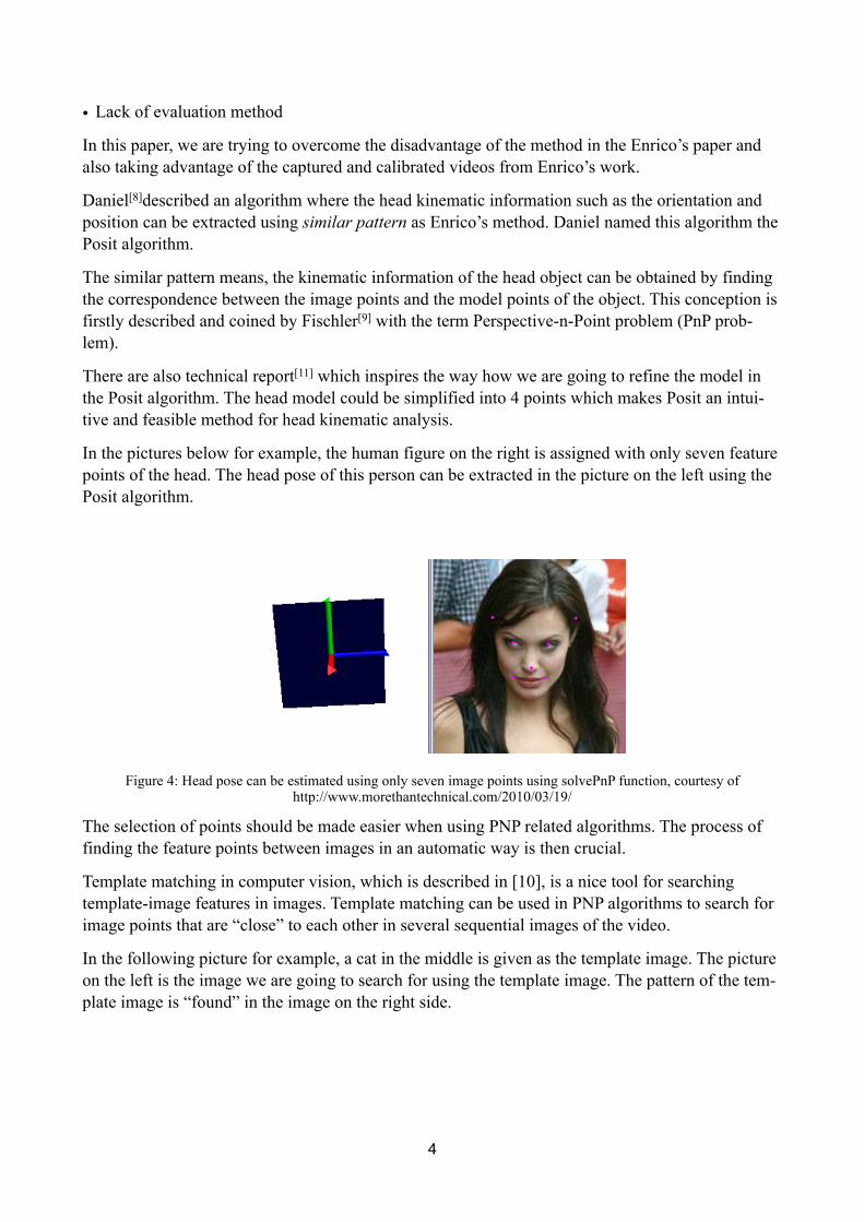
In the pictures below for example, the human figure on the right is assigned with only seven feature points of the head. The head pose of this person can be extracted in the picture on the left using the Posit algorithm.
Figure 4: Head pose can be estimated using only seven image points using solvePnP function, courtesy of http://www.morethantechnical.com/2010/03/19/
The selection of points should be made easier when using PNP related algorithms. The process of finding the feature points between images in an automatic way is then crucial.
Template matching in computer vision, which is described in [10], is a nice tool for searching template-image features in images. Template matching can be used in PNP algorithms to search for image points that are “close” to each other in several sequential images of the video.
In the following picture for example, a cat in the middle is given as the template image. The picture on the left is the image we are going to search for using the template image. The pattern of the tem-plate image is “found” in the image on the right side.
4
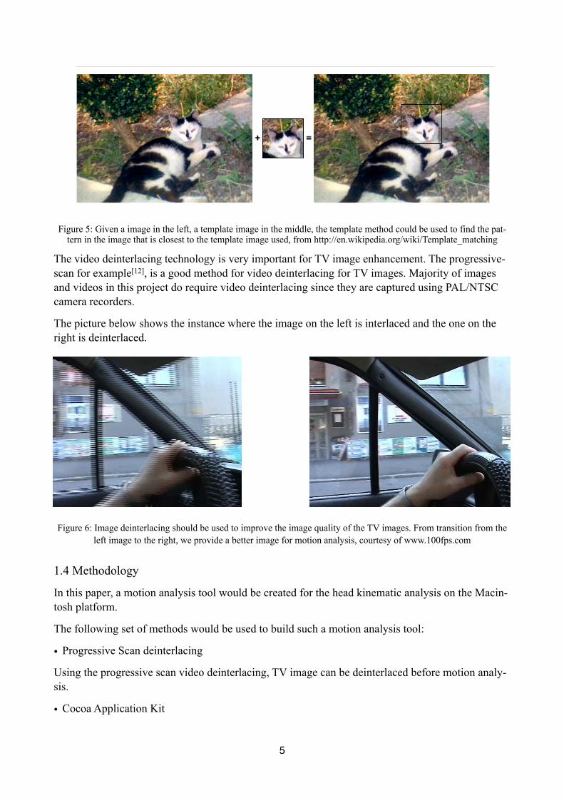
Figure 5: Given a image in the left, a template image in the middle, the template method could be used to find the pat-tern in the image that is closest to the template image used, from http://en.wikipedia.org/wiki/Template_matching
The video deinterlacing technology is very important for TV image enhancement. The progressive-scan for example[12], is a good method for video deinterlacing for TV images. Majority of images and videos in this project do require video deinterlacing since they are captured using PAL/NTSC camera recorders.
The picture below shows the instance where the image on the left is interlaced and the one on the right is deinterlaced.
Figure 6: Image deinterlacing should be used to improve the image quality of the TV images. From transition from the left image to the right, we provide a better image for motion analysis, courtesy of www.100fps.com
1.4 Methodology
In this paper, a motion analysis tool would be created for the head kinematic analysis on the Macin-tosh platform.
The following set of methods would be used to build such a motion analysis tool:
• Progressive Scan deinterlacing
Using the progressive scan video deinterlacing, TV image can be deinterlaced before motion analy-sis.
• Cocoa Application Kit
5
In order to build a motion analysis tool, user interface of the tool should be created and the event coming from mouse and keyboards should be handled. Cocoa Application Kit framework provided a way to perform this job.
User interface in the tool enables the user to perform various functionalities by clicking mouse to the buttons. These functionalities could include: loading the image, apply boxing linear filters, per-form dilation and erosion operation and undertake head pose analysis on the head object.
Event handling in the tool enables the user to handle mouse event and keyboard event coming from the window server in Mac OS X. The user might load pervious and next image in the image se-quence by sending mouse wheel event. Cocoa Application Kit makes this process possible and eas-ier.
• C++ standard template library
This project makes extensive use of standard libraries in C++. The most noticeable one is the usage of the std::vector class for high performance push back and referencing operations of feature points in the image.
• Drag and Drop Operation
Drag and drop operation is a facility in the Cocoa library in Mac OS X that enables us to load im-ages into the image analysis tool. Specifically speaking, the drag and drop operation triggers event during different stages of the drag session when the mouse is entering, moving and dropping into the Drag and Drop destinations. The image path names is passed into the event handler of these events and the image file can then be loaded
• Preferences
NSUserDefault class in Cocoa library helps saving the user preference of the motion analysis tool into the system preference database. The user preference could include the kernel size of the boxing filter in OpenCV, the block size of the adaptive thresholding, the operation type of the image mor-phology operation, the maximum level of hierarchy in the cvFindContours function and so on.
• OpenCV Image Processing Facility
In order to make the image analysis possible, the understanding of the image file and the operation that could be performed onto these files is necessary.
OpenCV library enables the understanding of image file by providing with image loading and im-age saving operations. Each image is represented by a C structure which is essentially a multi-dimensional matrix that saves the pixel data. The data could be either single channel or multi chan-nel which represents the gray scale image and color image respectively .
The functionality of OpenCV Image Processing facility includes the image blur operation, image morphology operation, image thresholding operation, Sobel and Canny operators, etc. The motion analysis tool created in this project combines these functionality into a single, unified user interface which the analyser can use for different purposes.
• OpenCV Posit Algorithm
Posit algorithm in OpenCV extracts the position and orientation of the object in the image by as-signing the image points and model points in the image. The rotation and translation matrices, as the
6

output of the Posit algorithm, reveals the head kinematic information of the object. The velocity of the object can also be captured with that piece of information.
Posit algorithm in OpenCV is the key technology used in this project where the technical details would be described in the following chapters.
• Matlab spline data interpolation
Matlab gives us a set of tools for the manipulation of the data obtained from the computer vision library. It enables developers to create a function with the input and output we desired. It provides the function to load the data file from the file system either row-wise or column-wise. New variable can be created in Matlab easily and when assigned to appropriate function, the output can be shown instantly to the user.
In this project, the spline function in Matlab is used for the spline data interpolation of the velocity data.
• Mac OS X Text System
In order to provide feedback information to the user, a logging system is created in the tool. The logging system takes fully advantage of the formatting syntax similar to the printf function in C li-brary.
NSMutableString class in Cocoa library enables the concatenation of formatted string onto the Log-ger console.
1.5 Structure of thesis
• Chapter 1 makes introduction of basic information of the thesis
• Chapter 2 tells about the theory and method of image preprocessing of research material
• Chapter 3 talks about the theory and method of kinematic analysis of research material
• Chapter 4 makes clear how the kinematic information can be obtain using the software developed
• Chapter 5 illustrates the accuracy of the motion analysis performed and make a comparison to re-lated studies
• Chapter 6 concludes the work undertaken and the delimitation which is found in the process of the study is revealed
7

2 VirtualDub video capture and OpenCV image preprocessing
2.1 Objective
Q: What is the definitions of the objects that we are going to analyse?
To understand the research problem, a clear definition of the objects we are going to analyse is es-sential.
A movie, or footage, or video, is a file in the computer system, which contains a set of sound tracks and video tracks. The video tracks of a movie can be exported to a set of images which represent the video content of the movie.
The frame-per-second, or FPS, is a crucial variable for time measurement, which is defined as the number of images that can be extracted from a video track of the movie in one second.
The image, from the perspective of the computer, is a file which contains a 2-dimensional array of brightness information. The array is a mapping from a point P in the space Ω to an intensity value denoted by I(x, y).
The space Ω is called the domain or size of the image. Since the image size in the movie is usually fixed, we can also call Ω the resolution of the movie.
Q: What is the objective of video capture and image preprocessing?
Video footages of different sports activities are fine materials for motion analysis. These footages has different resolutions, noise levels and frame rates.
This project makes analysis of a database which contains a set of box matching videos that are cap-tured in different locations and at different time. The content of these videos contains the knock-out hits between the two boxers. The head concussions and impacts of the head object during the hit is what we are going to analyze.
Before the image analysis of motions can be carried out, the image sequence must be captured from the sports video and the quality of image must be high enough for the motion analysis. These two preparation steps are called video capture and image preprocessing process. The objective of these processes can be further described as follows:
• The goal of video capture in this project is to obtain the image sequence from the video of differ-ent formats, deinterlace the TV image if necessary and try to improve the image quality during the image deinterlacing.
• The goal of image preprocessing is to create a image processing tool that give the opportunity for fine tuning the quality of the image which makes motion analysis easier.
8
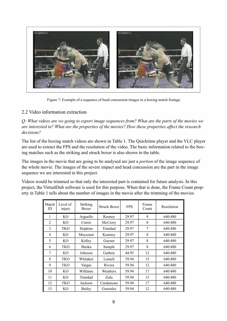
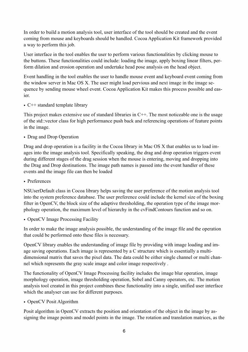
Figure 7: Example of a sequence of head concussion images in a boxing match footage
2.2 Video information extraction
Q: What videos are we going to export image sequences from? What are the parts of the movies we are interested in? What are the properties of the movies? How these properties affect the research decisions?
The list of the boxing match videos are shown in Table 1. The Quicktime player and the VLC player are used to extract the FPS and the resolution of the video. The basic information related to the box-ing matches such as the striking and struck boxer is also shown in the table.
The images in the movie that are going to be analysed are just a portion of the image sequence of the whole movie. The images of the severe impact and head concussion are the part in the image sequence we are interested in this project.
Videos would be trimmed so that only the interested part is contained for future analysis. In this project, the VirtualDub software is used for this purpose. When that is done, the Frame Count prop-erty in Table 1 tells about the number of images in the movie after the trimming of the movies.
MatchID
Level of injury
Striking Boxer Struck Boxer FPS Frame
Count Resolution
1 KO Arguello Rooney 29.97 9 640:4802 KO Currie McCrory 29.97 8 640:4803 TKO Hopkins Trinidad 29.97 7 640:4804 KO Maysonet Kearney 29.97 8 640:4805 KO Kelley Gayner 29.97 8 640:4806 TKO Sheika Sample 29.97 8 640:4807 KO Johnson Guthrie 44.95 12 640:4808 TKO Whitaker Lomeli 59.94 15 640:4809 TKO Vargas Rivera 59.94 12 640:480
10 KO Williams Weathers 59.94 17 640:48011 KO Trinidad Zulu 59.94 15 640:48012 TKO Jackson Cardamone 59.94 17 640:48013 KO Bailey Gonzalez 59.94 12 640:480
9

14 TKO Tua Izon 59.94 11 640:48015 KO Tua Chasteen 59.94 13 640:48016 KO Tua Ruiz 75 10 640:48017 KO Helenius Peter 75 16 704:40018 TKO Tackie Garcia 89.91 28 640:48019 KO Tua Nicholson 89.91 9 640:48020 KO Tyson Etienne 89.91 13 512:38421 KO McCallum Curry 89.91 19 640:48022 KO Lewis Tyson 89.91 12 352:24023 KO Pacquiao Hatton 89.91 11-20 640:36824 TKO Barkley Hearns 89.91 10 640:48025 TKO Olson Solis 89.91 9-15 640:480
Table 1: Listing of boxing match movies to be analyzed
2.3 Video deinterlacing, boosting and image sequence export using VirtualDub
Q: What is the quality of the video in this project? Why the video interlaced? What is the property of the interlaced video? Why video deinterlacing important?
After the visual inspection of the research videos, some of them has interlaced patterns that are sus-ceptible to interlaced videos. The interlaced videos are field-based videos which are usually cap-tured with a PAL or NTFS camera recorder. Each of the frames it captures contains two fields taken consecutively at time t1 and t2. The first field taken at t1 constructs the even line of the frame while the second field taken at t2 constructs the odd lines of the frame.
Considering the ideal case when the two fields of a frame is captured at the same time interval. The following equation would holds[12] for each of the frame in the movie:
t2 - t1 = 2 × FPS
This equation reveals that the field-based counterpart of the frame-based interlaced videos doubles the frame rate of the original video in this ideal situation.
The deinterlaced video which displayed on the Macbook 5.3 would have the interlaced pattern like the following:
10
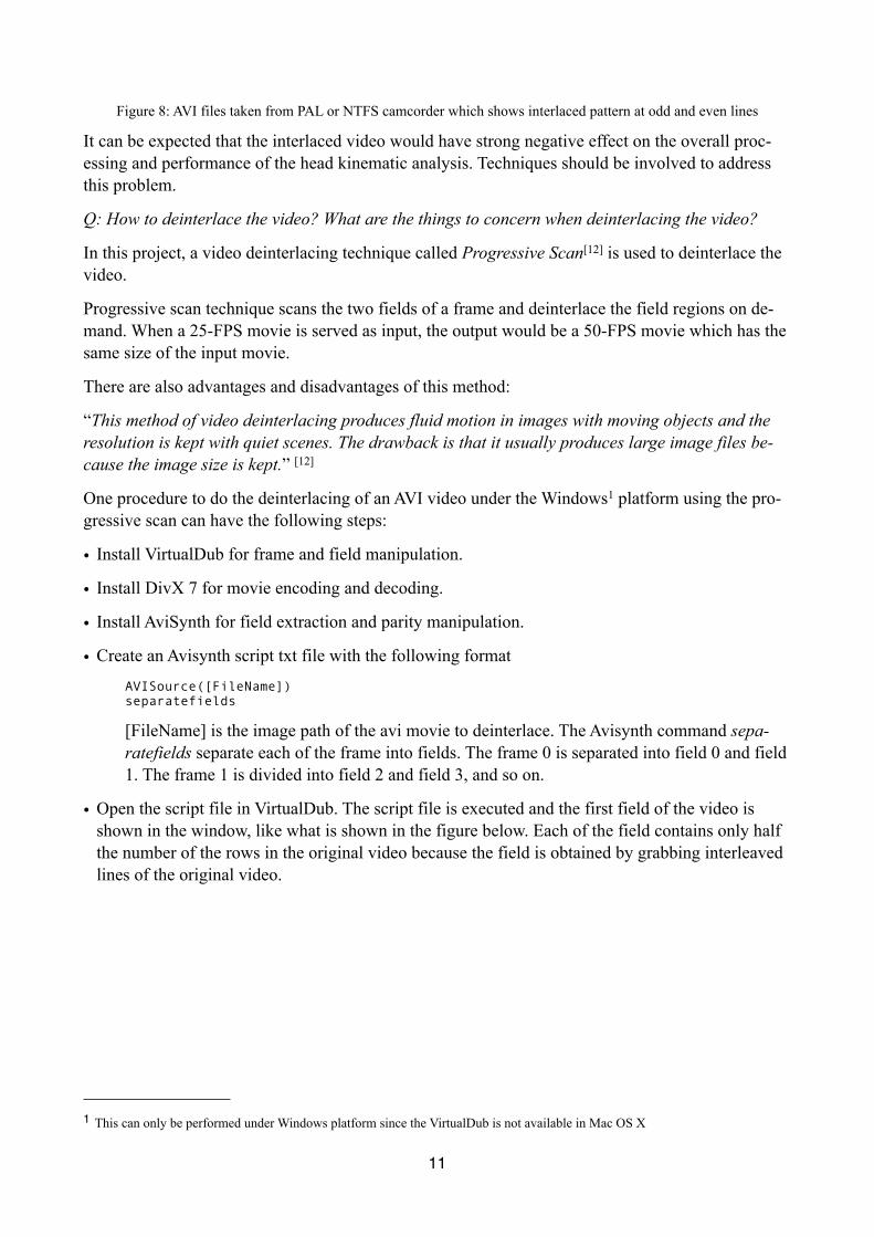
Figure 8: AVI files taken from PAL or NTFS camcorder which shows interlaced pattern at odd and even lines
It can be expected that the interlaced video would have strong negative effect on the overall proc-essing and performance of the head kinematic analysis. Techniques should be involved to address this problem.
Q: How to deinterlace the video? What are the things to concern when deinterlacing the video?
In this project, a video deinterlacing technique called Progressive Scan[12] is used to deinterlace the video.
Progressive scan technique scans the two fields of a frame and deinterlace the field regions on de-mand. When a 25-FPS movie is served as input, the output would be a 50-FPS movie which has the same size of the input movie.
There are also advantages and disadvantages of this method:
“This method of video deinterlacing produces fluid motion in images with moving objects and the resolution is kept with quiet scenes. The drawback is that it usually produces large image files be-cause the image size is kept.” [12]
One procedure to do the deinterlacing of an AVI video under the Windows1 platform using the pro-gressive scan can have the following steps:
• Install VirtualDub for frame and field manipulation.
• Install DivX 7 for movie encoding and decoding.
• Install AviSynth for field extraction and parity manipulation.
• Create an Avisynth script txt file with the following format
AVISource([FileName])separatefields
[FileName] is the image path of the avi movie to deinterlace. The Avisynth command sepa-ratefields separate each of the frame into fields. The frame 0 is separated into field 0 and field 1. The frame 1 is divided into field 2 and field 3, and so on.
• Open the script file in VirtualDub. The script file is executed and the first field of the video is shown in the window, like what is shown in the figure below. Each of the field contains only half the number of the rows in the original video because the field is obtained by grabbing interleaved lines of the original video.
11
1 This can only be performed under Windows platform since the VirtualDub is not available in Mac OS X
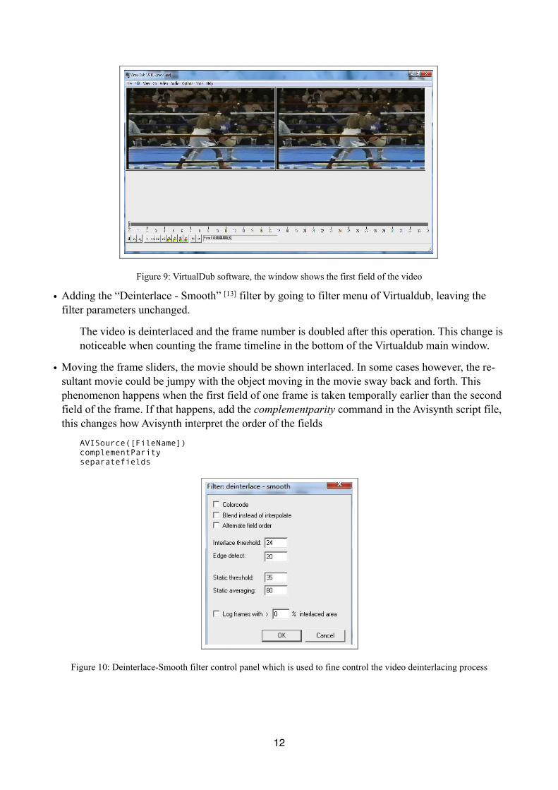
Figure 9: VirtualDub software, the window shows the first field of the video
• Adding the “Deinterlace - Smooth” [13] filter by going to filter menu of Virtualdub, leaving the filter parameters unchanged.
The video is deinterlaced and the frame number is doubled after this operation. This change is noticeable when counting the frame timeline in the bottom of the Virtualdub main window.
• Moving the frame sliders, the movie should be shown interlaced. In some cases however, the re-sultant movie could be jumpy with the object moving in the movie sway back and forth. This phenomenon happens when the first field of one frame is taken temporally earlier than the second field of the frame. If that happens, add the complementparity command in the Avisynth script file, this changes how Avisynth interpret the order of the fields
AVISource([FileName])complementParityseparatefields
Figure 10: Deinterlace-Smooth filter control panel which is used to fine control the video deinterlacing process
12
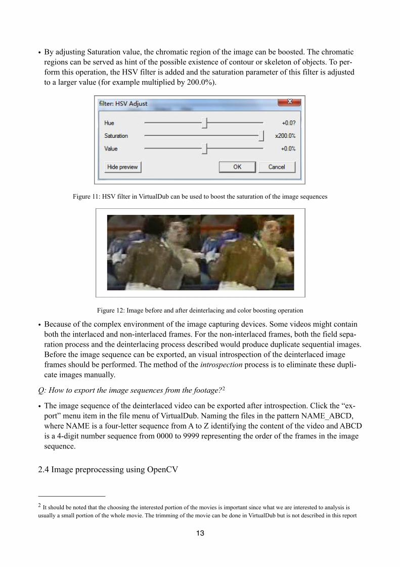
• By adjusting Saturation value, the chromatic region of the image can be boosted. The chromatic regions can be served as hint of the possible existence of contour or skeleton of objects. To per-form this operation, the HSV filter is added and the saturation parameter of this filter is adjusted to a larger value (for example multiplied by 200.0%).
Figure 11: HSV filter in VirtualDub can be used to boost the saturation of the image sequences
Figure 12: Image before and after deinterlacing and color boosting operation
• Because of the complex environment of the image capturing devices. Some videos might contain both the interlaced and non-interlaced frames. For the non-interlaced frames, both the field sepa-ration process and the deinterlacing process described would produce duplicate sequential images. Before the image sequence can be exported, an visual introspection of the deinterlaced image frames should be performed. The method of the introspection process is to eliminate these dupli-cate images manually.
Q: How to export the image sequences from the footage?2
• The image sequence of the deinterlaced video can be exported after introspection. Click the “ex-port” menu item in the file menu of VirtualDub. Naming the files in the pattern NAME_ABCD, where NAME is a four-letter sequence from A to Z identifying the content of the video and ABCD is a 4-digit number sequence from 0000 to 9999 representing the order of the frames in the image sequence.
2.4 Image preprocessing using OpenCV
13
2 It should be noted that the choosing the interested portion of the movies is important since what we are interested to analysis is usually a small portion of the whole movie. The trimming of the movie can be done in VirtualDub but is not described in this report

Q: After the image sequence has obtained from the video, why further improving the image quality? How to further improve the image in the image sequence? How to extract the useful image feature from the images?
When the image sequence with “good” quality is captured from the video, it is necessary to perform image processing operations on them. There are several reasons for this:
• There should be a way to load image sequences into memory and traverse the contents of the im-age sequence easily by sliding the mouse wheel back and forth
• Some of the videos in the database have high level of noise. OpenCV provides with low-pass fil-ters such as Gaussian and median filter which may be used to smooth the image so that the noise level of the image can be reduced.
• Binary image operations such as image thresholding, adaptive thresholding and canny operator are useful way to extract edge and contour information in the image. After adopting image thresh-olding in the human head surfaces for example, it would be easier to locate the eye center
• High level features such as line segments and contour trees can be extracted directly using hough transformation and Suzuki contour detector[14] in OpenCV.
• OpenCV provides with pose estimation algorithms that enables the estimation of head motion. It is natural to combine the feature extraction and motion tracking together in this tool.
• It is beneficial to combine the aforementioned features into a single toolbox
Motivated by the above statements, a tool called MotionTracker is developed implementing these features using OpenCV. It is developed under Mac OS X using Xcode with the following motiva-tions:
• There is a rich set of frameworks related to graphics under Mac OS X, which makes this platform a very good environment for image processing
• It is hard to find a OpenCV image processing tool that combines head motion tracking under Mac OS X, and preferably easy to use
14

Figure 13: Interface of MotionTracker tool
Q: What is the functionality of the image analysis tool used in the head kinematic analysis?
The functionality of MotionTracker can be summarized in the following table:
Functionality Class Description
Image Loading
Accessing Images
Load a path of images into memory
Image Traversing Accessing
Images
Traverse image sequences using slider or mouse wheel
Drag and Drop
Accessing Images A file contains set of images can be dragged directly into the interface for proc-
essing
Previous Image
Accessing Images
Select the previous image in the image sequence
Next Image
Accessing Images
Select the next image in the image sequence
Box Blur
Noise
Reduction
Convolve image with the variable sized boxing kernel, the image noise is sup-pressed[16]
Gaussian Blur Noise
Reduction
Convolve image with the variable sized Gaussian kernel, image noise is reduced, the image is sharper than the simple Box Blur
15
Functionality Class Description
Bilateral Blur
Noise
Reduction Convolve image with the variable sized bilateral kernel, image noise is reduced, the image has a painting effect after applying this filter
Median Blur
Noise
Reduction
Convolve image with the variable sized median kernel, image noise is reduced, edge pattern is better preserved applying this filter
Open
Image Morphol-
ogy
Breaks narrow isthmuses, and eliminates small islands and sharp peaks[23]
CloseImage
Morphol-ogy
Fuses narrow breaks and long thin gulfs and eliminates small holes[23]
Erode Image Morphol-
ogyShrink the region with low intensity
Dilate
Image Morphol-
ogy Expand the region with high intensity
TopHat
Image Morphol-
ogy
Highlights the region with higher intensity (white holes) than others
BlackHat
Image Morphol-
ogy
Highlights the region with lower intensity (black holes) than others
Basic Thresholding Image
Segmenta-tion
“Ones” or zeros the pixel in the fixed range of image intensity from the image
Adaptive Thresholding
ImageSegmenta-
tion “Ones” or zeros the pixel in the adaptive range of image intensity from the image
Canny Operator
ImageSegmenta-
tion
“Ones” image boundaries using derivative of the image functions, zeros others
Line Detector Feature Detector
Extract line patterns in the binary image
Contour Detector
Feature Detector
Extract contour sequences in the binary image
Model Assigner
Motion Tracker
Create, load, and save model created by assignment of points in the image
Posit pose es-timator Motion
Tracker
Estimate head or object poses using predefined head or object models. The yaw, pitch and roll value is extracted and demonstrated
Focal length estimator
Motion Tracker
Estimate the focal length using the Posit algorithm
Model Creator
Motion Tracker
Create the left and right ear model of the head object
MotionTracker Help Help The documentation that contains tutorials for the usage of the software
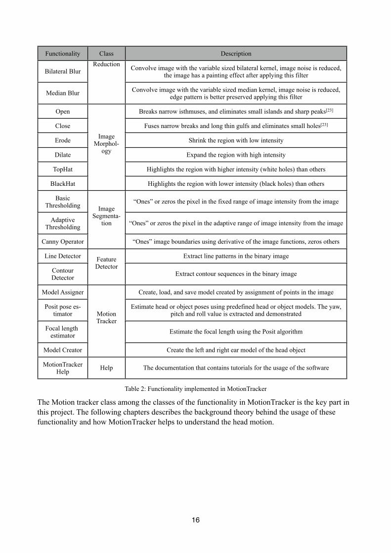
Table 2: Functionality implemented in MotionTracker
The Motion tracker class among the classes of the functionality in MotionTracker is the key part in this project. The following chapters describes the background theory behind the usage of these functionality and how MotionTracker helps to understand the head motion.
16

3 Head kinematic analysis with head pose estimation using Posit algorithm
3.1 Head pose estimation and head kinematics
Q: What is the rigid body kinematic analysis?
The rigid body in physics represents a body structure that the distance between any two points on the body remains constant regardless of the physical forces performs on it.[15]
The task of the rigid body kinematic analysis includes:
• Find the position of all of the points on the rigid body relative to the reference point
• Find the orientation of the rigid body relative to a reference frame
To obtain the position and orientation of 3D rigid objects, two coordinate systems would be intro-duced .
The first coordinate system is where the 3D modeling of the rigid object takes place. The 3D model of the rigid object describes the structure of it. The picture below, for instance, described a 3D model of the head. Each intersection of the meshes on the head is a point on the 3D head model. We would like to call the space where the 3D head model are defined the object coordinate system (OCS).
To analyse the motion of the object, it is necessary to introduce a reference coordinate system (RCS) which is fixed in the ground. The physical position of the head object is measured relative to the RCS. RCS defines and represents the world coordinates, where the motion of the object can be measured by locating the model points in RCS.
Figure 14: Example of the 3D model of the head. The points on the head lives in the space the we call the object coordi-nate system, courtesy of www.google.com
One category of method to perform the rigid body kinematic analysis is to discover the relationship between the point coordinate values living in RCS and OCS.
For example, one may prepare for the analysis of a head object by firstly constructing a 3D head model of a person in OCS, followed by finding the changes of these point coordinate values in the 2D image plane of RCS. When the head object is moving in the scene, the point coordinate values in RCS changes. The observation of the motion in RCS can be described in the following picture:
17
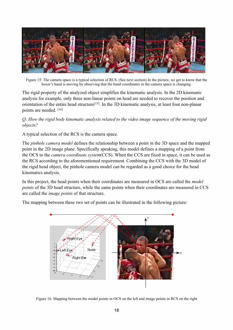
Figure 15: The camera space is a typical selection of RCS. (See next section) In the picture, we get to know that the boxer’s hand is moving by observing that the hand coordinates in the camera space is changing.
The rigid property of the analyzed object simplifies the kinematic analysis. In the 2D kinematic analysis for example, only three non-linear points on head are needed to recover the position and orientation of the entire head structure[15]. In the 3D kinematic analysis, at least four non-planar points are needed. [16]
Q: How the rigid body kinematic analysis related to the video image sequence of the moving rigid objects?
A typical selection of the RCS is the camera space.
The pinhole camera model defines the relationship between a point in the 3D space and the mapped point in the 2D image plane. Specifically speaking, this model defines a mapping of a point from the OCS to the camera coordinate system(CCS). When the CCS are fixed in space, it can be used as the RCS according to the aforementioned requirement. Combining the CCS with the 3D model of the rigid head object, the pinhole camera model can be regarded as a good choice for the head kinematics analysis.
In this project, the head points when their coordinates are measured in OCS are called the model points of the 3D head structure, while the same points when their coordinates are measured in CCS are called the image points of that structure.
The mapping between these two set of points can be illustrated in the following picture:
Figure 16: Mapping between the model points in OCS on the left and image points in RCS on the right
y
xo
18
On the right side, the image points in the CCS reveals the physical information of the head object, while the model points in the OCS on the left side defines the structure of it.
Q: What is the head pose estimation? How is it related to the head kinematic analysis?
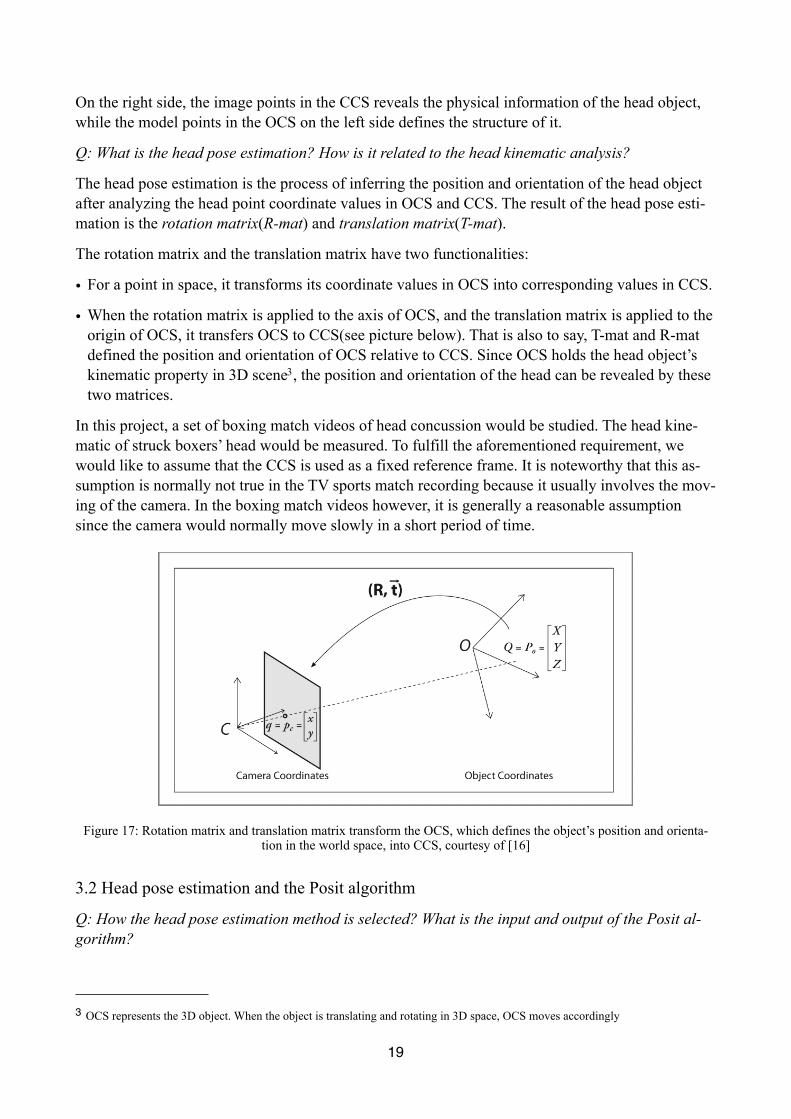
The head pose estimation is the process of inferring the position and orientation of the head object after analyzing the head point coordinate values in OCS and CCS. The result of the head pose esti-mation is the rotation matrix(R-mat) and translation matrix(T-mat).
The rotation matrix and the translation matrix have two functionalities:
• For a point in space, it transforms its coordinate values in OCS into corresponding values in CCS.
• When the rotation matrix is applied to the axis of OCS, and the translation matrix is applied to the origin of OCS, it transfers OCS to CCS(see picture below). That is also to say, T-mat and R-mat defined the position and orientation of OCS relative to CCS. Since OCS holds the head object’s kinematic property in 3D scene3, the position and orientation of the head can be revealed by these two matrices.
In this project, a set of boxing match videos of head concussion would be studied. The head kine-matic of struck boxers’ head would be measured. To fulfill the aforementioned requirement, we would like to assume that the CCS is used as a fixed reference frame. It is noteworthy that this as-sumption is normally not true in the TV sports match recording because it usually involves the mov-ing of the camera. In the boxing match videos however, it is generally a reasonable assumption since the camera would normally move slowly in a short period of time.
Figure 17: Rotation matrix and translation matrix transform the OCS, which defines the object’s position and orienta-tion in the world space, into CCS, courtesy of [16]
3.2 Head pose estimation and the Posit algorithm
Q: How the head pose estimation method is selected? What is the input and output of the Posit al-gorithm?
19
3 OCS represents the 3D object. When the object is translating and rotating in 3D space, OCS moves accordingly
Survey[17] has been conducted on the different methodologies of head pose estimations. One cate-gory of these methods are carried out by linking the human eye gazes with the head poses through visual gaze estimation. The gaze of the eye is characterized by the direction and focus of eyes. It should be reminded however, the TV images could failed to obtain enough resolution for the detec-tion of human eye’ focus, such as the footages in this project. This situation makes the methods of this category impractical in this project.
The Projection from Orthography and Scaling with ITerations (Posit) algorithm in OpenCV library is another head pose estimation method which is based on feature selection. The inputs and output of the algorithm makes it suitable for the head pose estimation in this project.
To use the Posit algorithm, two input arrays are needed. One of them is a pre-defined 3D model of the head, this is described with a vector of the head model points in OCS, denoted by M. The latter is the one-to-one mapped image points in CCS, denoted by I.
From the point of view of the computer language, the M and I vector can be defined using class NSDictionary in the AppKit framework in Mac OS X. The key of these two dictionaries is the de-scription of the points, whereas the object of these dictionaries is the coordinate value of the points corresponding to the keys. One example of the M and I array can be described by following tables:
Model Keys Model Objects
Left Eye (-12,0,13)
Right Eye (12,0,13)
Nose (0,0,0)
... ...
... ...
Table 3: Model Point Dictionary
Image Keys Image Objects
Left Eye (-87,28)
Right Eye (-34,32)
Nose (-43,34)
... ...
... ...
Table 4: Image Point Dictionary
Apart from M and I array, the camera focal length should also be determined in order to use the Posit algorithm. In this project, a fixed value of the focal length is used to do the motion analysis for boxing matches[delimitation 3.2]. A heuristic method that enables us to predict the input focal length of the Posit algorithm is created, but due to delimitation 3.2, this method is not used in the motion analysis process but used in the evaluation process of this project. The focal length prediction is de-scribed in Appendix I.
20
After the Posit algorithm has done its work, the output would be one 3 by 3 R-mat and one 3 by 1 T-mat. Discussions above tells us that these matrices reveal the location and orientation of the head object relative to the camera.
The R-mat and T-mat are denoted by Rij and Ti, where i and j represents the row and column indices respectively. 1 ≤ i ≤ 3 and 1 ≤ j ≤ 3.
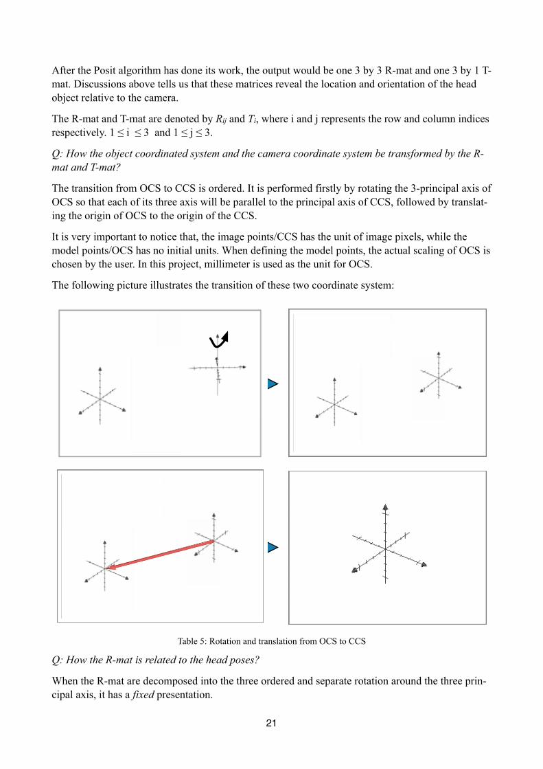
Q: How the object coordinated system and the camera coordinate system be transformed by the R-mat and T-mat?
The transition from OCS to CCS is ordered. It is performed firstly by rotating the 3-principal axis of OCS so that each of its three axis will be parallel to the principal axis of CCS, followed by translat-ing the origin of OCS to the origin of the CCS.
It is very important to notice that, the image points/CCS has the unit of image pixels, while the model points/OCS has no initial units. When defining the model points, the actual scaling of OCS is chosen by the user. In this project, millimeter is used as the unit for OCS.
The following picture illustrates the transition of these two coordinate system:
Table 5: Rotation and translation from OCS to CCS
Q: How the R-mat is related to the head poses?
When the R-mat are decomposed into the three ordered and separate rotation around the three prin-cipal axis, it has a fixed presentation.
21
Consider the OCS that is rotated by ! radians counter-clockwise around the z-axis, " radians counter-clockwise around the y-axis, and # radians counter-clockwise around the x-axis, the R-mat has the form of:
Ri,j = R(!,",#) = Rz(!)·Ry(")·Rx(#) = Ri,j = R(!,",#) = Rz(!)·Ry(")·Rx(#) = Ri,j = R(!,",#) = Rz(!)·Ry(")·Rx(#) =
cos!·cos" cos!·sin"·sin# - sin!·cos# cos!·sin"·cos# + sin!·sin#
sin!·cos" sin!·sin"·sin# + cos!·cos# sin!·sin"·cos# - cos!·sin#
-sin" cos"·sin# cos"·cos#
The R-mat that is represented after performing the rotation of the axis in the order of Z, Y and X axis is called the R-mat in Z-Y-X convention. When different orders are used, the representation of the R-mat would have to change. The Z-Y-X convention would be used in this project.
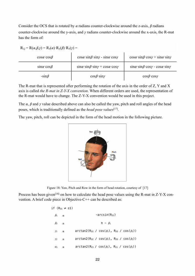
The !, " and # value described above can also be called the yaw, pitch and roll angles of the head poses, which is traditionally defined as the head pose values[17].
The yaw, pitch, roll can be depicted in the form of the head motion in the following picture.
Figure 18: Yaw, Pitch and Row in the form of head rotation, courtesy of [17]
Process has been given[18] on how to calculate the head pose values using the R-mat in Z-Y-X con-vention. A brief code piece in Objective-C++ can be described as:
if (R31 ≠ ±1)if (R31 ≠ ±1)if (R31 ≠ ±1)
"1 = -arcsin(R31)
"2 = π - "1
#1 = arctan2(R32 / cos("1), R33 / cos("1))
#2 = arctan2(R32 / cos("2), R33 / cos("2))
!1 = arctan2(R21 / cos("1), R11 / cos("1))
22
!2 = arctan2(R21 / cos("2), R11 / cos("2))
Notice that there are two possible combination of the head poses, (!1,"1,#1) and (!2,"2,#2) , they are representing the same head pose but with the different direction of rotation around the y-axis.
The first combination would be used in the project for clarity and simplicity.
To avoid the gimbal lock[19], the value of R31 is constrained to be not equal to ±1, which means the pitch value is defined not equal to 90 and -90 in degrees.
Q: How the T-mat related to the head poses?
The T-mat is performed on the origin of OCS after its rotation.
The 3 by 1 T-mat has the form of following:
Ti = { Tx Ty Tz } = OC
Define the origin of CCS as O, the origin of OCS as C. The T-mat represents the vector OC. Tx, Ty, Yz are the transitional component of the origin along the 3 principle axis of the camera coordinate system.
T-mat illustrates how “far” it is from the head object to the camera. For example, when the head is moving towards the center of the image space, Tx and Ty would be closer to 0. When the head is getting nearer to the camera, the value of Tz would expect to shrink.
Since T-mat describes distance information, Tx, Ty, Yz would be referred to the head distance val-ues in this report.
It is found that the units of the translation vector revealed by the Posit algorithm is the same as the unit of model points in OCS. This implies that the units of translation vector can be manually de-fined. It is obvious that keep in mind the units of T-mat is crucial in understanding the order of magnitude of the head translational movement.
Q: How to use the Posit algorithm in the REAL application? What are the steps?
The first step to use the Posit algorithm in the real head pose estimation application is to establish a 3D model of the head. The head model can usually be created by 3D modeling tools such as meshLab and Blender. The points in the 3D model is served as the model points in the Posit algo-rithm described above. They would be stored in the M array. In this project, a simplified head model is created using the method described in Appendix II.
In the second step, the image points corresponding to every model points are found in the image plane. They are stored in the I array for every image in the image sequence created in Chapter 2.
When step one and step two are done, M and I array can be illustrated in the table below.
In this project, the image points are selected using Model creation module in MotionTracker. The process of it will be discussed in Chapter 4.
23
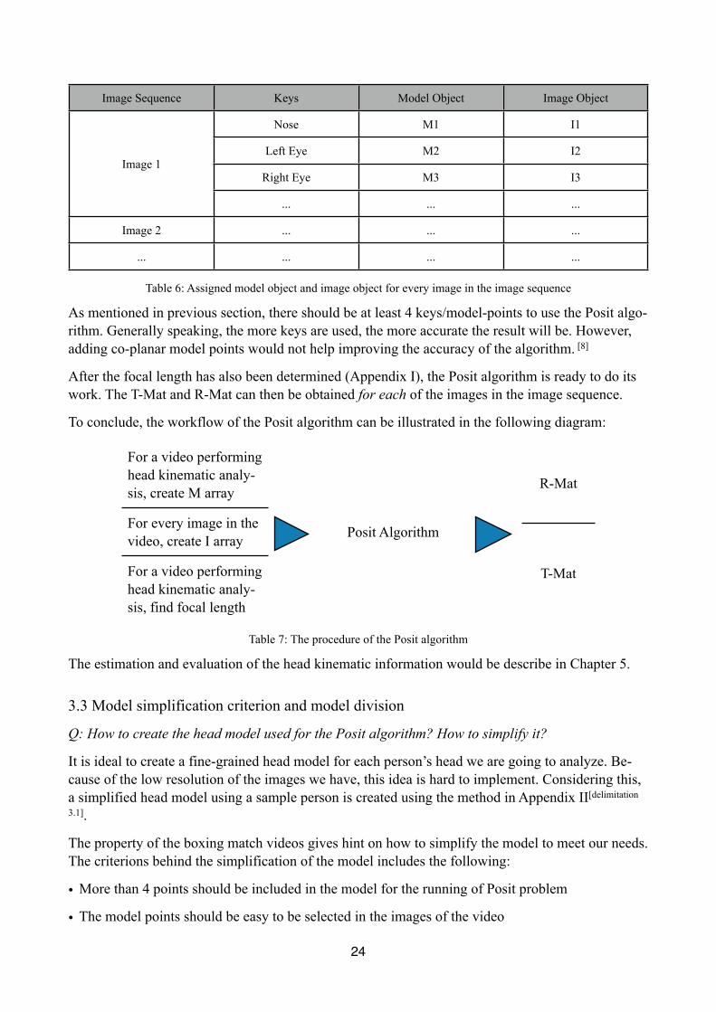
Image Sequence Keys Model Object Image Object
Image 1
Nose M1 I1
Image 1Left Eye M2 I2
Image 1Right Eye M3 I3
Image 1
... ... ...
Image 2 ... ... ...
... ... ... ...
Table 6: Assigned model object and image object for every image in the image sequence
As mentioned in previous section, there should be at least 4 keys/model-points to use the Posit algo-rithm. Generally speaking, the more keys are used, the more accurate the result will be. However, adding co-planar model points would not help improving the accuracy of the algorithm. [8]
After the focal length has also been determined (Appendix I), the Posit algorithm is ready to do its work. The T-Mat and R-Mat can then be obtained for each of the images in the image sequence.
To conclude, the workflow of the Posit algorithm can be illustrated in the following diagram:
For a video performing head kinematic analy-sis, create M array
R-Mat
For every image in the video, create I array Posit Algorithm
R-Mat
For every image in the video, create I array Posit Algorithm
T-MatFor a video performing head kinematic analy-sis, find focal length
T-Mat
Table 7: The procedure of the Posit algorithm
The estimation and evaluation of the head kinematic information would be describe in Chapter 5.
3.3 Model simplification criterion and model division
Q: How to create the head model used for the Posit algorithm? How to simplify it?
It is ideal to create a fine-grained head model for each person’s head we are going to analyze. Be-cause of the low resolution of the images we have, this idea is hard to implement. Considering this, a simplified head model using a sample person is created using the method in Appendix II[delimitation
3.1].
The property of the boxing match videos gives hint on how to simplify the model to meet our needs. The criterions behind the simplification of the model includes the following:
• More than 4 points should be included in the model for the running of Posit problem
• The model points should be easy to be selected in the images of the video
24
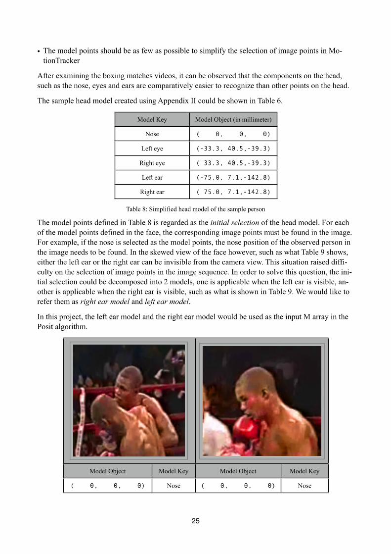
• The model points should be as few as possible to simplify the selection of image points in Mo-tionTracker
After examining the boxing matches videos, it can be observed that the components on the head, such as the nose, eyes and ears are comparatively easier to recognize than other points on the head.
The sample head model created using Appendix II could be shown in Table 6.
Model Key Model Object (in millimeter)
Nose ( 0, 0, 0)
Left eye (-33.3, 40.5,-39.3)
Right eye ( 33.3, 40.5,-39.3)
Left ear (-75.0, 7.1,-142.8)
Right ear ( 75.0, 7.1,-142.8)
Table 8: Simplified head model of the sample person
The model points defined in Table 8 is regarded as the initial selection of the head model. For each of the model points defined in the face, the corresponding image points must be found in the image. For example, if the nose is selected as the model points, the nose position of the observed person in the image needs to be found. In the skewed view of the face however, such as what Table 9 shows, either the left ear or the right ear can be invisible from the camera view. This situation raised diffi-culty on the selection of image points in the image sequence. In order to solve this question, the ini-tial selection could be decomposed into 2 models, one is applicable when the left ear is visible, an-other is applicable when the right ear is visible, such as what is shown in Table 9. We would like to refer them as right ear model and left ear model.
In this project, the left ear model and the right ear model would be used as the input M array in the Posit algorithm.
Model Object Model Key Model Object Model Key
( 0, 0, 0) Nose ( 0, 0, 0) Nose
25
(-33.3, 40.5,-39.3) Left eye (-33.3, 40.5,-39.3) Left eye
( 33.3, 40.5,-39.3) Right eye ( 33.3, 40.5,-39.3) Right eye
( 75.0, 7.1,-142.8) Right ear (-75.0, 7.1,-142.8) Left ear
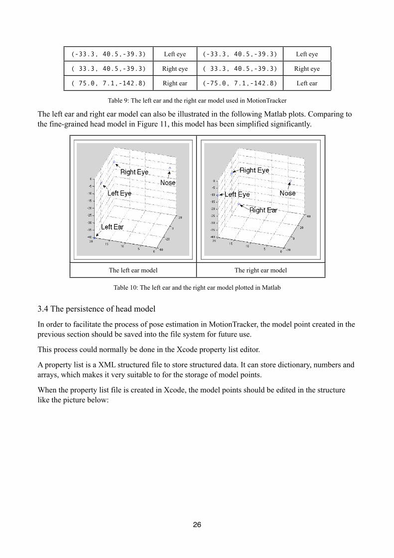
Table 9: The left ear and the right ear model used in MotionTracker
The left ear and right ear model can also be illustrated in the following Matlab plots. Comparing to the fine-grained head model in Figure 11, this model has been simplified significantly.
The left ear model The right ear model
Table 10: The left ear and the right ear model plotted in Matlab
3.4 The persistence of head model
In order to facilitate the process of pose estimation in MotionTracker, the model point created in the previous section should be saved into the file system for future use.
This process could normally be done in the Xcode property list editor.
A property list is a XML structured file to store structured data. It can store dictionary, numbers and arrays, which makes it very suitable to for the storage of model points.
When the property list file is created in Xcode, the model points should be edited in the structure like the picture below:
26
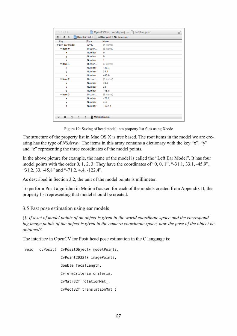
Figure 19: Saving of head model into property list files using Xcode
The structure of the property list in Mac OS X is tree based. The root items in the model we are cre-ating has the type of NSArray. The items in this array contains a dictionary with the key “x”, “y” and “z” representing the three coordinates of the model points.
In the above picture for example, the name of the model is called the “Left Ear Model”. It has four model points with the order 0, 1, 2, 3. They have the coordinates of “0, 0, 1”, “-31.1, 33.1, -45.9”, “31.2, 33, -45.8” and “-71.2, 4.4, -122.4”.
As described in Section 3.2, the unit of the model points is millimeter.
To perform Posit algorithm in MotionTracker, for each of the models created from Appendix II, the property list representing that model should be created.
3.5 Fast pose estimation using ear models
Q: If a set of model points of an object is given in the world coordinate space and the correspond-ing image points of the object is given in the camera coordinate space, how the pose of the object be obtained?
The interface in OpenCV for Posit head pose estimation in the C language is:
void cvPosit( CvPositObject* modelPoints,
CvPoint2D32f* imagePoints,
double focalLength,
CvTermCriteria criteria,
CvMatr32f rotationMat_,
CvVect32f translationMat_)
27

Here, modelPoints is the input M dictionary, imagePoints is the input I dictionary, focalLength is the input focus length, rotationMat_ and translationMat_ is the output R-mat and T-mat.
Q: How the face pose values and head distance value be obtain using the C interface of the Posit algorithm where the definition of both can be found in Section 3.2?
When the R-mat is obtained, the head pose values can be obtained by the following lines of C code,
yaw = -asinf(rotationMat_[6]);
pitch = atan2(rotationMat_[7] / cos(yaw), rotationMat_[8] / cos(yaw));
row = atan2(rotationMat_[3] / cos(yaw), rotationMat_[0] / cos(yaw));
While head distance values can be illustrated by:
tx = translationMat_[0];
ty = translationMat_[1];
tz = translationMat_[2];
Q: How does the selection of model related to the usage of Posit algorithm?
R-mat and T-mat are calculated according to the input of the algorithm. When different models are used, different result would be given. It is generally a bad idea to find the relationship between the transition matrices calculated using different models.
The creation and selection of the model is based on the property of the image for analysis. In the simplified model such as the left and right ear model for instance, the one that is going to be chosen as the input for the algorithm depends on the accessibility of the corresponding point in the image. Specifically speaking, when the left ear is accessible from the image, left ear model is used; when the right ear model is accessible, right ear model is used.
28

4 Posit head pose estimation in MotionTracker
4.1 Objective
The MotionTracker Posit module is the place where the head pose estimation is actually carried out.
MotionTracker helps the running of the Posit algorithm in the following ways:
• MotionTracker can load image folder which contains a set of ordered images using drag and drop operation.
• MotionTracker can load the 3D head model from the model property file and store it in the M ar-ray.
• MotionTracker creates the files for each image in the image sequence for storing image points and store it in the I array.
• MotionTracker supports the visual editing of I array on image
• MotionTracker helps the assignment of the focal length and FPS of the movies used for motion calculation.
• MotionTracker performs the Posit algorithm
• MotionTracker represents the result of the R-mat and T-mat about head orientation and position.
• MotionTracker represents the rotation speed and translation speed of head
The process of the Posit head pose estimation in MotionTracker includes the following steps:
• Load the images in the image sequence
• Load the model points in the property list file
• Load the image points in the OpenCV XML file of the images
• Edit the image points using MotionTracker model creator
• Compute the head pose according to the model and image points using the Posit algorithm
• Representation of the result of head motion
In this chapter, the steps of the Posit head pose estimation in MotionTracker will be discussed in detail.
4.2 The loading of inputs of Posit algorithm with drag-and-drop operation
Chapter 2, Section 2.3 described the method to obtain the image sequence of a video. The image sequence is represented as a list of PNG files in the file system. In order to make the video analysis easier, these image files are put into one folder.
Before the image folder is loaded into MotionTracker, the property list file of the model(Section 3.4) should also be added to the image folder.
29
As mentioned in Section 3.3, the head model used in this project are either right ear model or left ear model. They are represented by two property list files created by Xcode. To determine whether the left ear model or right ear model should be used, the image sequence should be inspected to see if the right or the left ear is occluded from the camera. It is obvious that the right ear model should be chosen if the left ear is occluded and vice versa.
In the analysed videos, it is uncommon but possible that both the struck boxers’ ear can be occluded from the camera, we make a compromise in [delimitation 4.1] the process here so that the “less occluded” model is chosen.
After the appropriate model is chosen, the property file of that model is put into the image folder.
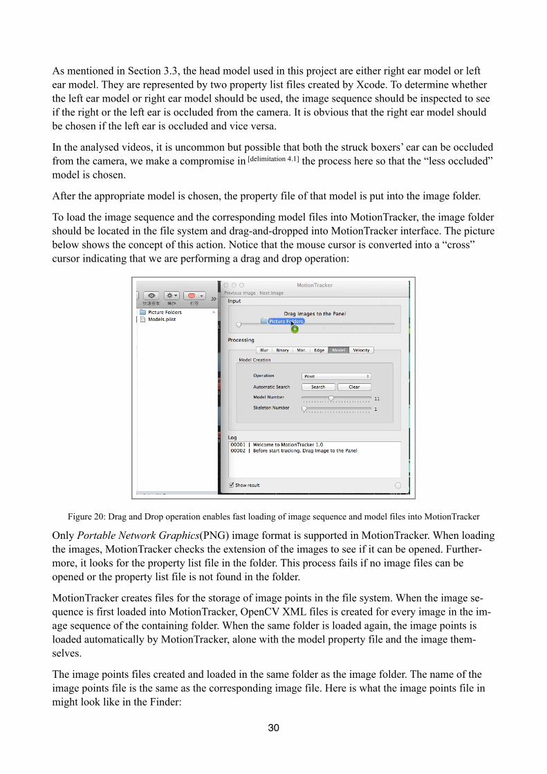
To load the image sequence and the corresponding model files into MotionTracker, the image folder should be located in the file system and drag-and-dropped into MotionTracker interface. The picture below shows the concept of this action. Notice that the mouse cursor is converted into a “cross” cursor indicating that we are performing a drag and drop operation:
Figure 20: Drag and Drop operation enables fast loading of image sequence and model files into MotionTracker
Only Portable Network Graphics(PNG) image format is supported in MotionTracker. When loading the images, MotionTracker checks the extension of the images to see if it can be opened. Further-more, it looks for the property list file in the folder. This process fails if no image files can be opened or the property list file is not found in the folder.
MotionTracker creates files for the storage of image points in the file system. When the image se-quence is first loaded into MotionTracker, OpenCV XML files is created for every image in the im-age sequence of the containing folder. When the same folder is loaded again, the image points is loaded automatically by MotionTracker, alone with the model property file and the image them-selves.
The image points files created and loaded in the same folder as the image folder. The name of the image points file is the same as the corresponding image file. Here is what the image points file in might look like in the Finder:
30
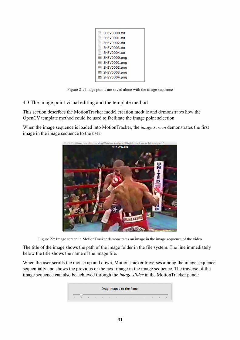
Figure 21: Image points are saved alone with the image sequence
4.3 The image point visual editing and the template method
This section describes the MotionTracker model creation module and demonstrates how the OpenCV template method could be used to facilitate the image point selection.
When the image sequence is loaded into MotionTracker, the image screen demonstrates the first image in the image sequence to the user:
Figure 22: Image screen in MotionTracker demonstrates an image in the image sequence of the video
The title of the image shows the path of the image folder in the file system. The line immediately below the title shows the name of the image file.
When the user scrolls the mouse up and down, MotionTracker traverses among the image sequence sequentially and shows the previous or the next image in the image sequence. The traverse of the image sequence can also be achieved through the image slider in the MotionTracker panel:
31
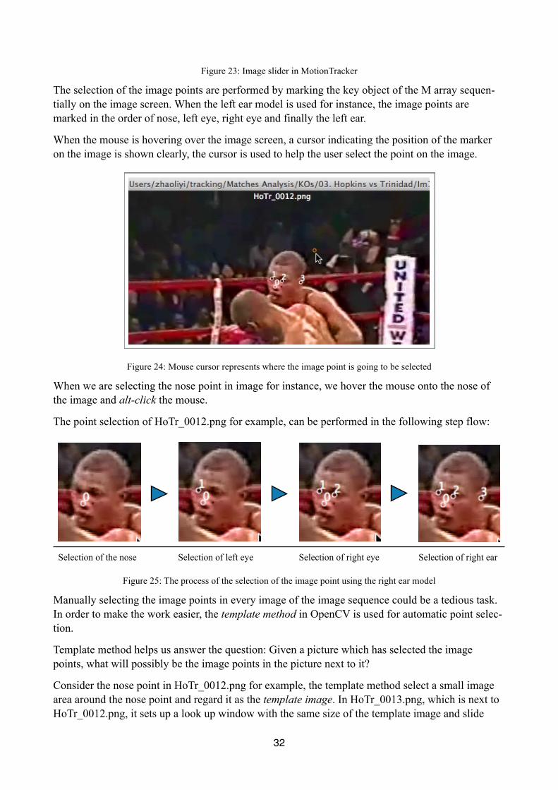
Figure 23: Image slider in MotionTracker
The selection of the image points are performed by marking the key object of the M array sequen-tially on the image screen. When the left ear model is used for instance, the image points are marked in the order of nose, left eye, right eye and finally the left ear.
When the mouse is hovering over the image screen, a cursor indicating the position of the marker on the image is shown clearly, the cursor is used to help the user select the point on the image.
Figure 24: Mouse cursor represents where the image point is going to be selected
When we are selecting the nose point in image for instance, we hover the mouse onto the nose of the image and alt-click the mouse.
The point selection of HoTr_0012.png for example, can be performed in the following step flow:
Selection of the nose Selection of left eye Selection of right eye Selection of right ear
Figure 25: The process of the selection of the image point using the right ear model
Manually selecting the image points in every image of the image sequence could be a tedious task. In order to make the work easier, the template method in OpenCV is used for automatic point selec-tion.
Template method helps us answer the question: Given a picture which has selected the image points, what will possibly be the image points in the picture next to it?
Consider the nose point in HoTr_0012.png for example, the template method select a small image area around the nose point and regard it as the template image. In HoTr_0013.png, which is next to HoTr_0012.png, it sets up a look up window with the same size of the template image and slide
32
through whole image area. It computes the difference between template image and the sliding win-dow, and finds the one that is closest to the template image according to some method. The avail-able comparison method includes:
Method Description
CV_TM_SQDIFF The squared difference is computed between the template and the image. 0 for perfect match.
CV_TM_CCORR The multiplicative of the template against the image is used. Large value for better match.
CV_TM_CCOEFFTemplate relative to its mean is match against the image relative to its mean. 1 is perfect match. -1 is perfect mis-match. 0 is no correlation
Table 11: The way the template image is compared to the sliding window in the template method
The square difference method is used in this project.
The pseudo code of the template method can be described as:
Set index = 0For index from 0 to the number of image points in the current image$ Finds the image point P with index index$ Finds the window rect roi_rect around the P with width and height selected as 20$ Obtain the template image of the current image using roi_rect$ Match template image against the next image, obtain the comparison matrix(CM)$ Obtain location of the point in the next image where CM has the minimum value$ index = index + 1
To select the image point automatically, we completely select the image points in one image of the image sequence, then choose the next image using either the mouse wheel or the image slider. After that, we can choose the “search” button in the MotionTracker panel asking it to select the image point of the second image for us:
Figure 26: Automatic image point searching option in MotionTracker with the usage of template method
The capability to edit the image point is a crucial convenience method for the creation of image points in MotionTracker.
The editing of image points can be performed easily by selecting the created image points on the image screen. And drag the point around the image screen to the desired position. The same opera-tion can also be done by pressing the arrow keys in the keyboard when they are available to use. A typical usage of this operation can be illustrated in the following picture:
33
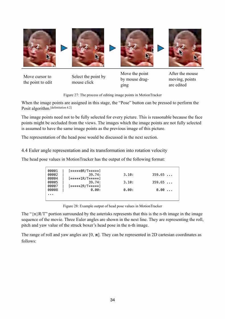
Move cursor to the point to edit
Select the point by mouse click
Move the point by mouse drag-ging
After the mouse moving, points are edited
Figure 27: The process of editing image points in MotionTracker
When the image points are assigned in this stage, the “Pose” button can be pressed to perform the Posit algorithm.[delimitation 4.2]
The image points need not to be fully selected for every picture. This is reasonable because the face points might be occluded from the views. The images which the image points are not fully selected is assumed to have the same image points as the previous image of this picture.
The representation of the head pose would be discussed in the next section.
4.4 Euler angle representation and its transformation into rotation velocity
The head pose values in MotionTracker has the output of the following format:
Figure 28: Example output of head pose values in MotionTracker
The “{n}R/T” portion surrounded by the asterisks represents that this is the n-th image in the image sequence of the movie. Three Euler angles are shown in the next line. They are representing the roll, pitch and yaw value of the struck boxer’s head pose in the n-th image.
The range of roll and yaw angles are [0, $]. They can be represented in 2D cartesian coordinates as follows:
00001 | [*****0R/T*****]00002 | 39.74: 3.10: 359.65 ...00004 | [*****1R/T*****]00005 | 39.74: 3.10: 359.65 ...00007 | [*****2R/T*****]00008 | 0.00: 0.00: 0.00 ......
34
Figure 29: Representation of roll and yaw values in 2D cartesian space in MotionTracker
The range of pitch angles are [-0.5$, 0.5$]. They can be represented in 2D cartesian coordinates as follows:
Figure 30: Representation of pitch values in 2D cartesian space in MotionTracker
Suppose roll angle is !1 in the (i)-th image, and !2 in the (i+1)-th image, the angular velocity of the roll angle from the (i)-th image to the (i+1)-th image could be computed in the pseudo code like fol-lows:
find the absolute delta of a1 - a2, so delta = abs(a1 - a2)if delta is bigger than pi$ delta = 2 * pi - delta;the angular velocity V along x-axis is calculated as delta / (1. / FPS)if(a2 - a1 < 0) and the delta is smaller than pi$ the head is moving along x-axis clockwise in the velocity Velse$ the head is moving along x-axis counter-clockwise in the velocity V
The concern regarding the delta of !1 and !2 is raised because it is hard for MotionTracker to tell whether the head is rotating clockwise or counter-clockwise only referring to the Euler angles. This property is determined by the value of abs(!2 - !1) and (!2 - !1) altogether, where the rotation is de-fined always in the direction with a absolute delta value smaller than $.[delimitation 4.3]
The angular velocity of the yaw angle can be calculated in the similar way as the roll angle. Substi-tuting the alpha value with the gamma value would be sufficient.
The calculation of pitch angle is easier because the direction of rotation is only determined by the delta of the pitch values.
35
Suppose pitch angle is "1 in the (i)-th image, and "2 in the (i+1)-th image, the angular velocity of the pitch angle from the (i)-th image to the (i+1)-th image could be computed in the pseudo code like follows:
find the absolute delta of b1 - b2, so delta = abs(b1 - b2)the angular velocity V along y-axis is calculated as delta / (1. / FPS)if(a2 - a1 < 0)$ the head is moving along y-axis clockwise in the velocity Velse$ the head is moving along y-axis counter-clockwise in the velocity V
The result of the angular velocity calculation has the following pattern of output in MotionTracker:
z rotation speed0.0000000.0000000.000000-7.317708-0.447545-25.5662021.67584020.3226476.8258485.96572646.5081790.0000000.000000
We can see from the output that it represents the angular rotation velocity around the z-axis. From the 7th image to the 8th image for example, it is estimated that the head is rotating around z-axis at the velocity of 46.508179 rad/s.
4.5 Translation representation and its transformation into translation velocity
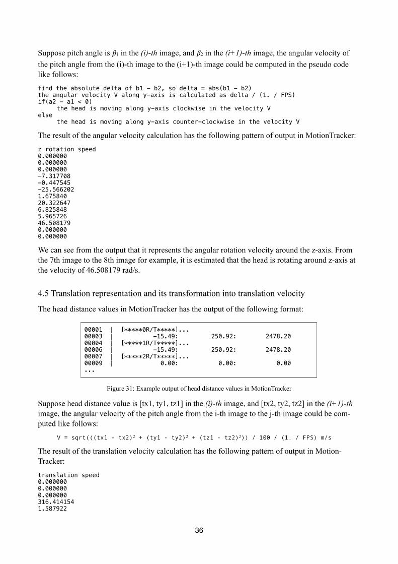
The head distance values in MotionTracker has the output of the following format:
Figure 31: Example output of head distance values in MotionTracker
Suppose head distance value is [tx1, ty1, tz1] in the (i)-th image, and [tx2, ty2, tz2] in the (i+1)-th image, the angular velocity of the pitch angle from the i-th image to the j-th image could be com-puted like follows:
V = sqrt(((tx1 - tx2)2 + (ty1 - ty2)2 + (tz1 - tz2)2)) / 100 / (1. / FPS) m/s
The result of the translation velocity calculation has the following pattern of output in Motion-Tracker:
translation speed0.0000000.0000000.000000316.4141541.587922
00001 | [*****0R/T*****]...00003 | -15.49: 250.92: 2478.2000004 | [*****1R/T*****]...00006 | -15.49: 250.92: 2478.2000007 | [*****2R/T*****]...00009 | 0.00: 0.00: 0.00...
36

40.23540585.2972413.20073719.54186451.49530813.0009010.0000000.000000
37
5 Head rotation estimation and evaluation
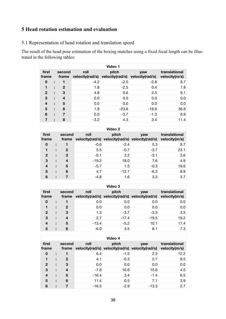
5.1 Representation of head rotation and translation speed
The result of the head pose estimation of the boxing matches using a fixed focal length can be illus-trated in the following tables:
Video 1Video 1Video 1first
framesecond frame
Video 1Video 1Video 1Video 1roll
velocity(rad/s)pitch
velocity(rad/s)yaw
velocity(rad/s)translational velocity(m/s)
0 : 11 : 22 : 33 : 44 : 55 : 66 : 77 : 8
-4.2 -2.0 -2.8 8.71.8 -2.5 0.4 7.84.8 0.6 2.5 9.10.0 0.0 0.0 0.00.0 0.0 0.0 0.01.9 -23.6 -16.6 36.90.0 -3.7 -1.3 6.9-3.2 4.3 3.4 11.4
Video 2Video 2Video 2first
framesecond frame
Video 2Video 2Video 2Video 2roll
velocity(rad/s)pitch
velocity(rad/s)yaw
velocity(rad/s)translational velocity(m/s)
0 : 11 : 22 : 33 : 44 : 55 : 66 : 7
-0.6 -2.4 5.3 9.75.5 -0.7 -3.7 23.1-0.1 3.2 -3.1 3.6
-19.2 18.0 7.6 4.9-5.7 1.5 -0.3 19.64.7 -12.7 -6.3 8.9-4.8 1.6 3.3 3.7
Video 3Video 3Video 3first
framesecond frame
Video 3Video 3Video 3Video 3roll
velocity(rad/s)pitch
velocity(rad/s)yaw
velocity(rad/s)translational velocity(m/s)
0 : 11 : 22 : 33 : 44 : 55 : 6
0.0 0.0 0.0 0.00.0 0.0 0.0 0.01.3 -3.7 -3.3 3.52.7 -17.4 -19.5 19.2
-13.4 -5.2 10.1 17.4-6.0 3.5 8.1 7.3
Video 4Video 4Video 4first
framesecond frame
Video 4Video 4Video 4Video 4roll
velocity(rad/s)pitch
velocity(rad/s)yaw
velocity(rad/s)translational velocity(m/s)
0 : 11 : 22 : 33 : 44 : 55 : 66 : 7
6.4 -1.3 2.3 12.24.1 -0.3 2.7 8.50.0 0.0 0.0 0.0-7.6 16.6 15.6 4.5
-16.4 3.4 -1.4 6.511.4 0.5 7.1 3.9-16.5 -2.9 -13.3 2.7
38
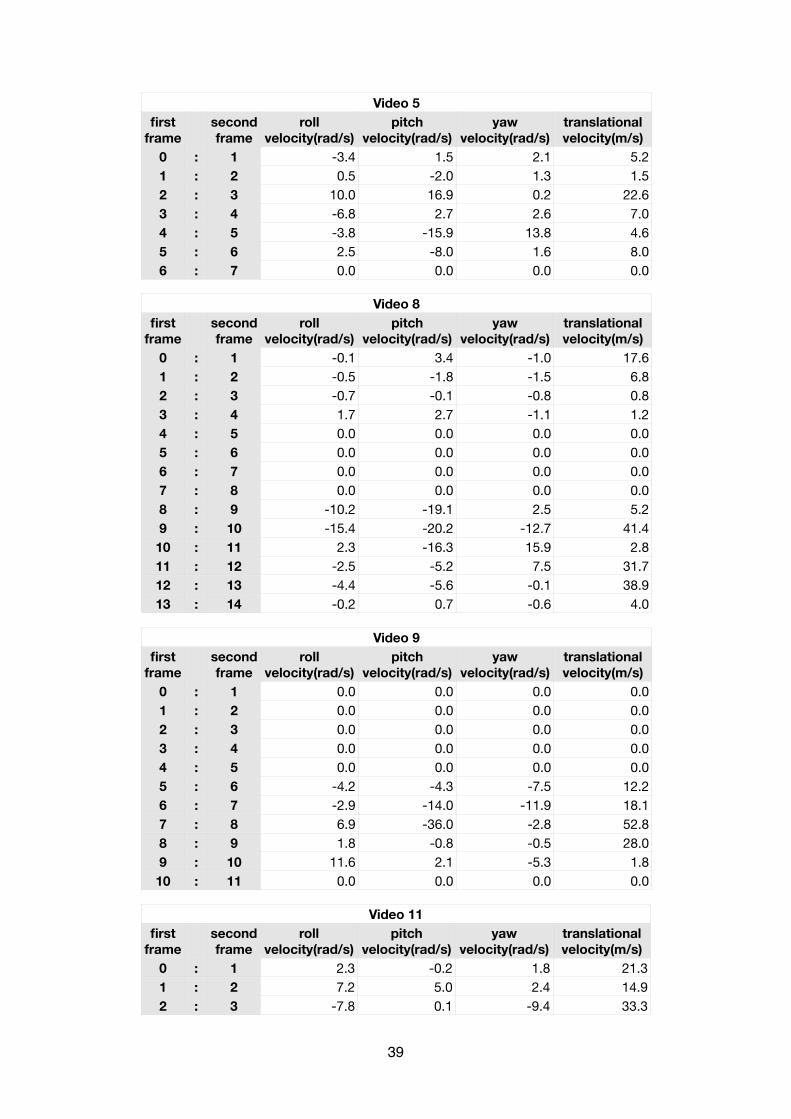
Video 5Video 5Video 5first
framesecond frame
Video 5Video 5Video 5Video 5roll
velocity(rad/s)pitch
velocity(rad/s)yaw
velocity(rad/s)translational velocity(m/s)
0 : 11 : 22 : 33 : 44 : 55 : 66 : 7
-3.4 1.5 2.1 5.20.5 -2.0 1.3 1.5
10.0 16.9 0.2 22.6-6.8 2.7 2.6 7.0-3.8 -15.9 13.8 4.62.5 -8.0 1.6 8.00.0 0.0 0.0 0.0
Video 8Video 8Video 8first
framesecond frame
Video 8Video 8Video 8Video 8roll
velocity(rad/s)pitch
velocity(rad/s)yaw
velocity(rad/s)translational velocity(m/s)
0 : 11 : 22 : 33 : 44 : 55 : 66 : 77 : 88 : 99 : 1010 : 1111 : 1212 : 1313 : 14
-0.1 3.4 -1.0 17.6-0.5 -1.8 -1.5 6.8-0.7 -0.1 -0.8 0.81.7 2.7 -1.1 1.20.0 0.0 0.0 0.00.0 0.0 0.0 0.00.0 0.0 0.0 0.00.0 0.0 0.0 0.0
-10.2 -19.1 2.5 5.2-15.4 -20.2 -12.7 41.42.3 -16.3 15.9 2.8-2.5 -5.2 7.5 31.7-4.4 -5.6 -0.1 38.9-0.2 0.7 -0.6 4.0
Video 9Video 9Video 9first
framesecond frame
Video 9Video 9Video 9Video 9roll
velocity(rad/s)pitch
velocity(rad/s)yaw
velocity(rad/s)translational velocity(m/s)
0 : 11 : 22 : 33 : 44 : 55 : 66 : 77 : 88 : 99 : 1010 : 11
0.0 0.0 0.0 0.00.0 0.0 0.0 0.00.0 0.0 0.0 0.00.0 0.0 0.0 0.00.0 0.0 0.0 0.0-4.2 -4.3 -7.5 12.2-2.9 -14.0 -11.9 18.16.9 -36.0 -2.8 52.81.8 -0.8 -0.5 28.0
11.6 2.1 -5.3 1.80.0 0.0 0.0 0.0
Video 11Video 11Video 11first
framesecond frame
Video 11Video 11Video 11Video 11roll
velocity(rad/s)pitch
velocity(rad/s)yaw
velocity(rad/s)translational velocity(m/s)
0 : 11 : 22 : 3
2.3 -0.2 1.8 21.37.2 5.0 2.4 14.9-7.8 0.1 -9.4 33.3
39
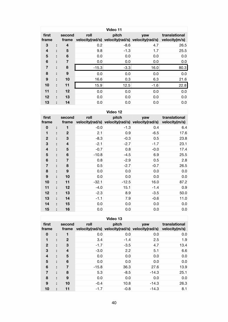
Video 11Video 11Video 11first
framesecond frame
Video 11Video 11Video 11Video 11roll
velocity(rad/s)pitch
velocity(rad/s)yaw
velocity(rad/s)translational velocity(m/s)
3 : 44 : 55 : 66 : 77 : 88 : 99 : 1010 : 1111 : 1212 : 1313 : 14
0.2 -8.6 4.7 26.59.8 -1.3 1.7 25.50.0 0.0 0.0 0.00.0 0.0 0.0 0.0
-15.3 -3.3 16.0 80.30.0 0.0 0.0 0.0
16.6 0.3 6.3 21.615.9 12.5 -1.6 22.80.0 0.0 0.0 0.00.0 0.0 0.0 0.00.0 0.0 0.0 0.0
Video 12Video 12Video 12first
framesecond frame
Video 12Video 12Video 12Video 12roll
velocity(rad/s)pitch
velocity(rad/s)yaw
velocity(rad/s)translational velocity(m/s)
0 : 11 : 22 : 33 : 44 : 55 : 66 : 77 : 88 : 99 : 1010 : 1111 : 1212 : 1313 : 1414 : 1515 : 16
-0.0 -1.3 0.4 6.42.1 0.9 -6.5 17.6-8.3 -0.3 0.5 23.8-2.1 -2.7 -1.7 23.1-0.7 0.8 -0.0 17.4
-10.8 -4.5 6.9 25.50.8 -2.9 0.5 2.80.5 -2.7 -0.7 26.50.0 0.0 0.0 0.00.0 0.0 0.0 0.0
-32.1 -12.5 16.0 87.2-4.0 15.1 -1.4 0.9-2.3 8.9 -3.5 50.0-1.1 7.9 -0.6 11.00.0 0.0 0.0 0.00.0 0.0 0.0 0.0
Video 13Video 13Video 13first
framesecond frame
Video 13Video 13Video 13Video 13roll
velocity(rad/s)pitch
velocity(rad/s)yaw
velocity(rad/s)translational velocity(m/s)
0 : 11 : 22 : 33 : 44 : 55 : 66 : 77 : 88 : 99 : 1010 : 11
0.0 0.0 0.0 0.03.4 -1.4 2.5 1.9-1.7 -3.5 4.7 13.4-3.0 2.2 5.1 6.60.0 0.0 0.0 0.00.0 0.0 0.0 0.0
-15.8 36.3 27.6 13.95.3 -8.5 -14.3 25.10.0 0.0 0.0 0.0-0.4 10.8 -14.3 26.3-1.7 -0.8 -14.3 8.1
40
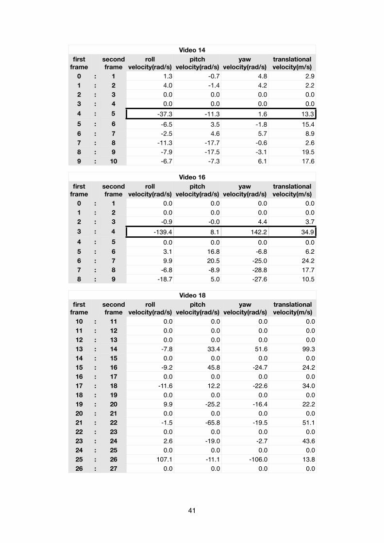
Video 14Video 14Video 14first
framesecond frame
Video 14Video 14Video 14Video 14roll
velocity(rad/s)pitch
velocity(rad/s)yaw
velocity(rad/s)translational velocity(m/s)
0 : 11 : 22 : 33 : 44 : 55 : 66 : 77 : 88 : 99 : 10
1.3 -0.7 4.8 2.94.0 -1.4 4.2 2.20.0 0.0 0.0 0.00.0 0.0 0.0 0.0
-37.3 -11.3 1.6 13.3-6.5 3.5 -1.8 15.4-2.5 4.6 5.7 8.9
-11.3 -17.7 -0.6 2.6-7.9 -17.5 -3.1 19.5-6.7 -7.3 6.1 17.6
Video 16Video 16Video 16first
framesecond frame
Video 16Video 16Video 16Video 16roll
velocity(rad/s)pitch
velocity(rad/s)yaw
velocity(rad/s)translational velocity(m/s)
0 : 11 : 22 : 33 : 44 : 55 : 66 : 77 : 88 : 9
0.0 0.0 0.0 0.00.0 0.0 0.0 0.0
-0.9 -0.0 4.4 3.7-139.4 8.1 142.2 34.9
0.0 0.0 0.0 0.03.1 16.8 -6.8 6.29.9 20.5 -25.0 24.2
-6.8 -8.9 -28.8 17.7-18.7 5.0 -27.6 10.5
Video 18Video 18Video 18first
framesecond frame
Video 18Video 18Video 18Video 18roll
velocity(rad/s)pitch
velocity(rad/s)yaw
velocity(rad/s)translational velocity(m/s)
10 : 1111 : 1212 : 1313 : 1414 : 1515 : 1616 : 1717 : 1818 : 1919 : 2020 : 2121 : 2222 : 2323 : 2424 : 2525 : 2626 : 27
0.0 0.0 0.0 0.00.0 0.0 0.0 0.00.0 0.0 0.0 0.0
-7.8 33.4 51.6 99.30.0 0.0 0.0 0.0
-9.2 45.8 -24.7 24.20.0 0.0 0.0 0.0
-11.6 12.2 -22.6 34.00.0 0.0 0.0 0.09.9 -25.2 -16.4 22.20.0 0.0 0.0 0.0
-1.5 -65.8 -19.5 51.10.0 0.0 0.0 0.02.6 -19.0 -2.7 43.60.0 0.0 0.0 0.0
107.1 -11.1 -106.0 13.80.0 0.0 0.0 0.0
41
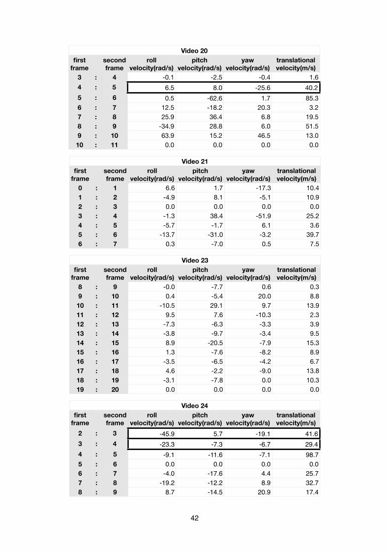
Video 20Video 20Video 20first
framesecond frame
Video 20Video 20Video 20Video 20roll
velocity(rad/s)pitch
velocity(rad/s)yaw
velocity(rad/s)translational velocity(m/s)
3 : 44 : 55 : 66 : 77 : 88 : 99 : 1010 : 11
-0.1 -2.5 -0.4 1.66.5 8.0 -25.6 40.20.5 -62.6 1.7 85.3
12.5 -18.2 20.3 3.225.9 36.4 6.8 19.5-34.9 28.8 6.0 51.563.9 15.2 46.5 13.00.0 0.0 0.0 0.0
Video 21Video 21Video 21first
framesecond frame
Video 21Video 21Video 21Video 21roll
velocity(rad/s)pitch
velocity(rad/s)yaw
velocity(rad/s)translational velocity(m/s)
0 : 11 : 22 : 33 : 44 : 55 : 66 : 7
6.6 1.7 -17.3 10.4-4.9 8.1 -5.1 10.90.0 0.0 0.0 0.0-1.3 38.4 -51.9 25.2-5.7 -1.7 6.1 3.6
-13.7 -31.0 -3.2 39.70.3 -7.0 0.5 7.5
Video 23Video 23Video 23first
framesecond frame
Video 23Video 23Video 23Video 23roll
velocity(rad/s)pitch
velocity(rad/s)yaw
velocity(rad/s)translational velocity(m/s)
8 : 99 : 1010 : 1111 : 1212 : 1313 : 1414 : 1515 : 1616 : 1717 : 1818 : 1919 : 20
-0.0 -7.7 0.6 0.30.4 -5.4 20.0 8.8
-10.5 29.1 9.7 13.99.5 7.6 -10.3 2.3-7.3 -6.3 -3.3 3.9-3.8 -9.7 -3.4 9.58.9 -20.5 -7.9 15.31.3 -7.6 -8.2 8.9-3.5 -6.5 -4.2 6.74.6 -2.2 -9.0 13.8-3.1 -7.8 0.0 10.30.0 0.0 0.0 0.0
Video 24Video 24Video 24first
framesecond frame
Video 24Video 24Video 24Video 24roll
velocity(rad/s)pitch
velocity(rad/s)yaw
velocity(rad/s)translational velocity(m/s)
2 : 33 : 44 : 55 : 66 : 77 : 88 : 9
-45.9 5.7 -19.1 41.6-23.3 -7.3 -6.7 29.4
-9.1 -11.6 -7.1 98.70.0 0.0 0.0 0.0
-4.0 -17.6 4.4 25.7-19.2 -12.2 8.9 32.7
8.7 -14.5 20.9 17.4
42
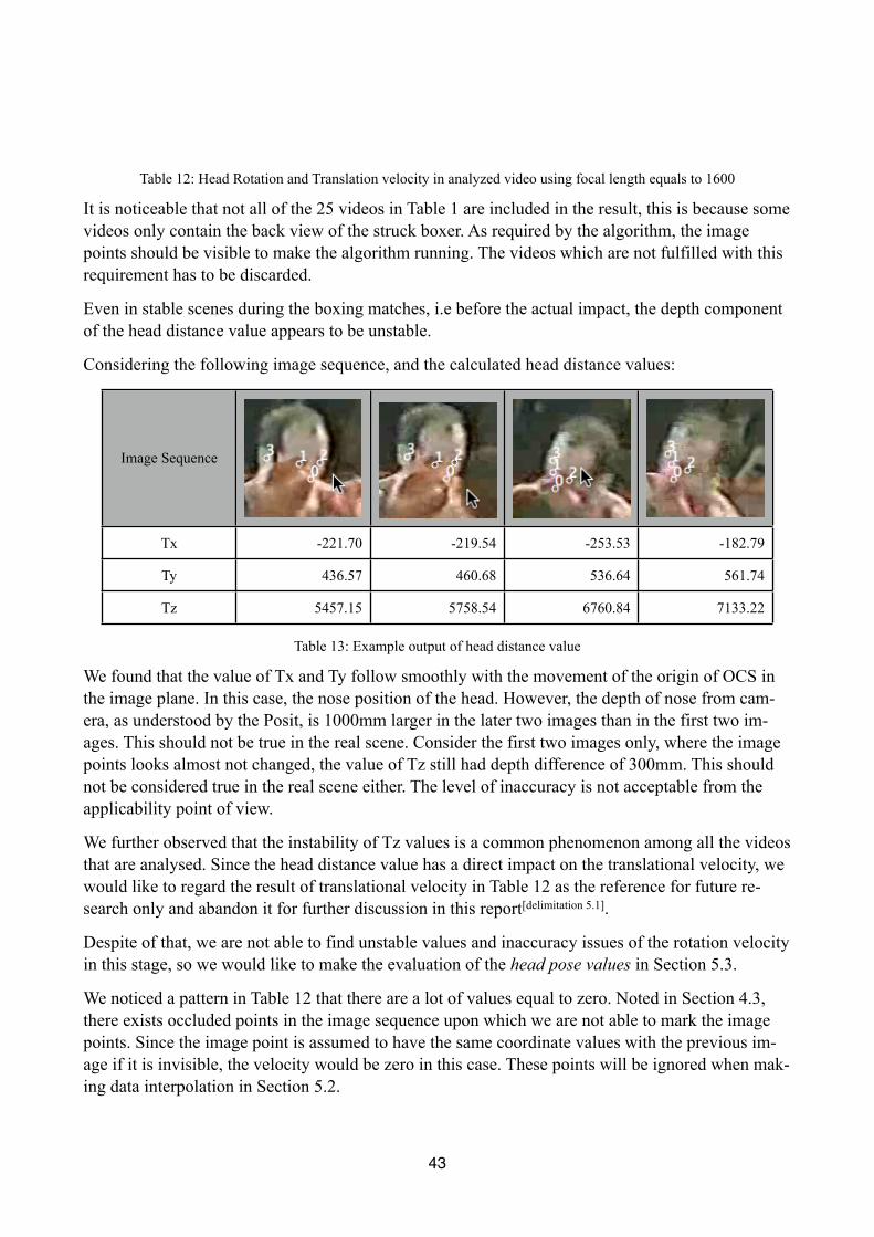
Table 12: Head Rotation and Translation velocity in analyzed video using focal length equals to 1600
It is noticeable that not all of the 25 videos in Table 1 are included in the result, this is because some videos only contain the back view of the struck boxer. As required by the algorithm, the image points should be visible to make the algorithm running. The videos which are not fulfilled with this requirement has to be discarded.
Even in stable scenes during the boxing matches, i.e before the actual impact, the depth component of the head distance value appears to be unstable.
Considering the following image sequence, and the calculated head distance values:
Image Sequence
Tx -221.70 -219.54 -253.53 -182.79
Ty 436.57 460.68 536.64 561.74
Tz 5457.15 5758.54 6760.84 7133.22
Table 13: Example output of head distance value
We found that the value of Tx and Ty follow smoothly with the movement of the origin of OCS in the image plane. In this case, the nose position of the head. However, the depth of nose from cam-era, as understood by the Posit, is 1000mm larger in the later two images than in the first two im-ages. This should not be true in the real scene. Consider the first two images only, where the image points looks almost not changed, the value of Tz still had depth difference of 300mm. This should not be considered true in the real scene either. The level of inaccuracy is not acceptable from the applicability point of view.
We further observed that the instability of Tz values is a common phenomenon among all the videos that are analysed. Since the head distance value has a direct impact on the translational velocity, we would like to regard the result of translational velocity in Table 12 as the reference for future re-search only and abandon it for further discussion in this report[delimitation 5.1].
Despite of that, we are not able to find unstable values and inaccuracy issues of the rotation velocity in this stage, so we would like to make the evaluation of the head pose values in Section 5.3.
We noticed a pattern in Table 12 that there are a lot of values equal to zero. Noted in Section 4.3, there exists occluded points in the image sequence upon which we are not able to mark the image points. Since the image point is assumed to have the same coordinate values with the previous im-age if it is invisible, the velocity would be zero in this case. These points will be ignored when mak-ing data interpolation in Section 5.2.
43

From direct observation of the pitch velocity shown in Table 12, we found there are some incorrect assignment of the direction of velocity after comparing with the supposed direction in the image sequence. The susceptible values are shown in Table 12 with the bold rectangle around them. We believe this is a consequence of gimbal lock since the incorrect value always take place when the head got a comparatively large pitch value relative to the camera. The evaluation part in Section 5.3 further proved and explained the existence of the gimbal lock issue. The table below shows one of these situation when a struck boxer’s face is hit. During this impact, the head pitch velocity is ex-pected to be positive, but the estimation given in Motiontracker is negative.
Image Sequence
Pitch Velocity -11.3-11.3
5.2 The interpolation of the velocity data
In order to obtain a better representation of the result, the velocity data can be further smoothed us-ing cubic spline data interpolation in Matlab. A Matlab function is created for this purpose:
function r = motiontrack( fps, datapath, granularity, titles, xlabels, ylabels, extent )%MOTIONTRACK given fps, datapath and granularity% Compute the spline of the data% fps is the frame rate of the video% datapath is the path of the datafile%return% return the array of the spline data using granularity%note% choose granularity larger than 100% choose extent 10 to 100 datas = load([datapath, '.txt']); switch titles case 'Head Rotation X' datas = datas(1, :); case 'Head Rotation Y' datas = datas(2, :); case 'Head Rotation Z' datas = datas(3, :); end; t = 0:(1/fps):((length(datas)-1)/fps); newt = t(1) : t(end)/granularity: t(end); newdatas = spline(t, datas, newt); r = newdatas; %save switch titles case 'Head Rotation X' save([datapath, 'X'], 'newdatas'); figure_n = 1; case 'Head Rotation Y' save([datapath, 'Y'], 'newdatas'); figure_n = 2; case 'Head Rotation Z' save([datapath, 'Z'], 'newdatas');
44
figure_n = 3; end; %plot figure(figure_n); plot(t, datas, 'o', newt, newdatas); title(titles); xlabel(xlabels); ylabel(ylabels); axis([t(1) t(end) ((min([min(newdatas) min(datas)])) - extent) ((max([max(newdatas) max(datas)])) + extent)]); saveas(figure_n, [datapath, titles, '.png']);end
Firstly, the data file containing the velocity data with respect to the x-y-z axis is created in a single file. This file has the format of:
-45.87 -23.29 -9.09 -4.01 -19.18 8.735.73 -7.26 -11.56 -17.60 -12.20 -14.48-19.06 -6.67 -7.13 4.37 8.94 20.94
The first row records roll angular velocity. The second row records the pitch angular velocity. The third row records the yaw angular velocity.
In the next step, the data file is loaded into Matlab, the FPS and granularity of the output graph is assigned. The spline function, as shown below, has three parameters. The first parameter is the time frame of the velocity function. This is calculated using the FPS assigned. “Datas” are velocity val-ues indicated in the velocity data file. The interpolant is assigned as the third parameter of this func-tion which defines the time frame of velocity function it wants to interpolate into.
newdatas = spline(t, datas, newt);
Finally, the graph of the splined function and the interpolated data is saved into the file system.
The spline new interval, as assigned in the third parameter of the spline function, is 100 in this pro-ject.
After the data has been interpolated, the roll, pitch and yaw angular velocity can be depicted as the following picture for the video 1 instance:
45
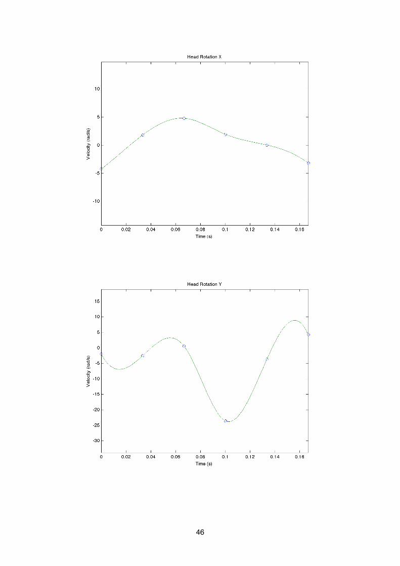
46
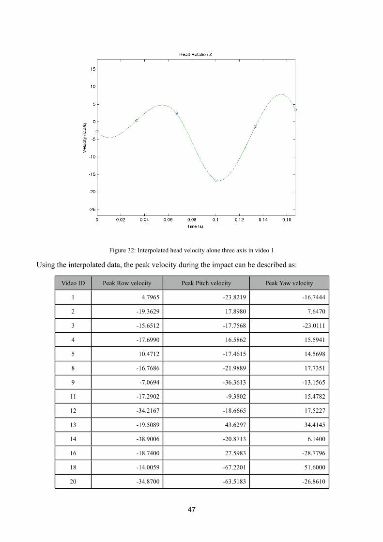
Figure 32: Interpolated head velocity alone three axis in video 1
Using the interpolated data, the peak velocity during the impact can be described as:
Video ID Peak Row velocity Peak Pitch velocity Peak Yaw velocity
1 4.7965 -23.8219 -16.7444
2 -19.3629 17.8980 7.6470
3 -15.6512 -17.7568 -23.0111
4 -17.6990 16.5862 15.5941
5 10.4712 -17.4615 14.5698
8 -16.7686 -21.9889 17.7351
9 -7.0694 -36.3613 -13.1565
11 -17.2902 -9.3802 15.4782
12 -34.2167 -18.6665 17.5227
13 -19.5089 43.6297 34.4145
14 -38.9006 -20.8713 6.1400
16 -18.7400 27.5983 -28.7796
18 -14.0059 -67.2201 51.6000
20 -34.8700 -63.5183 -26.8610
47
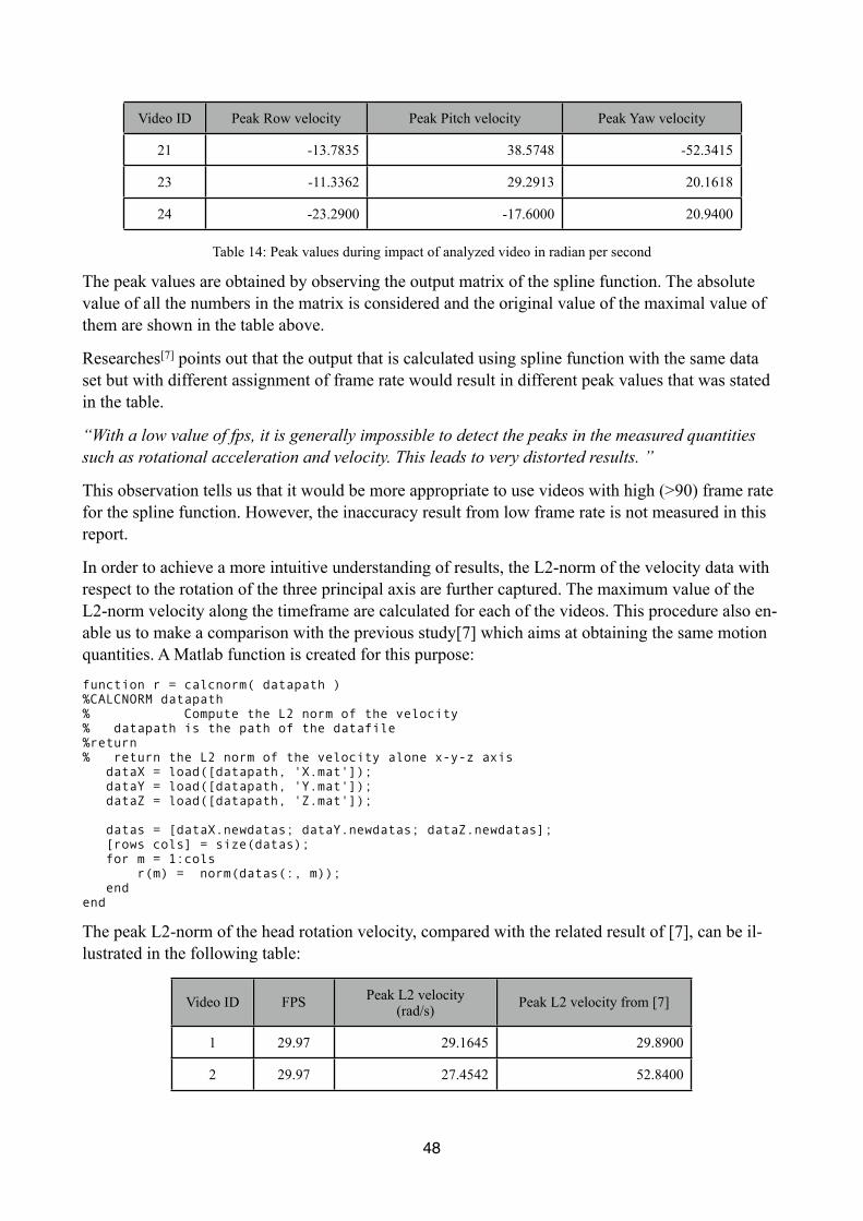
Video ID Peak Row velocity Peak Pitch velocity Peak Yaw velocity
21 -13.7835 38.5748 -52.3415
23 -11.3362 29.2913 20.1618
24 -23.2900 -17.6000 20.9400
Table 14: Peak values during impact of analyzed video in radian per second
The peak values are obtained by observing the output matrix of the spline function. The absolute value of all the numbers in the matrix is considered and the original value of the maximal value of them are shown in the table above.
Researches[7] points out that the output that is calculated using spline function with the same data set but with different assignment of frame rate would result in different peak values that was stated in the table.
“With a low value of fps, it is generally impossible to detect the peaks in the measured quantities such as rotational acceleration and velocity. This leads to very distorted results. ”
This observation tells us that it would be more appropriate to use videos with high (>90) frame rate for the spline function. However, the inaccuracy result from low frame rate is not measured in this report.
In order to achieve a more intuitive understanding of results, the L2-norm of the velocity data with respect to the rotation of the three principal axis are further captured. The maximum value of the L2-norm velocity along the timeframe are calculated for each of the videos. This procedure also en-able us to make a comparison with the previous study[7] which aims at obtaining the same motion quantities. A Matlab function is created for this purpose:
function r = calcnorm( datapath )%CALCNORM datapath % Compute the L2 norm of the velocity% datapath is the path of the datafile%return% return the L2 norm of the velocity alone x-y-z axis dataX = load([datapath, 'X.mat']); dataY = load([datapath, 'Y.mat']); dataZ = load([datapath, 'Z.mat']); datas = [dataX.newdatas; dataY.newdatas; dataZ.newdatas]; [rows cols] = size(datas); for m = 1:cols r(m) = norm(datas(:, m)); endend
The peak L2-norm of the head rotation velocity, compared with the related result of [7], can be il-lustrated in the following table:
Video ID FPS Peak L2 velocity(rad/s) Peak L2 velocity from [7]
1 29.97 29.1645 29.8900
2 29.97 27.4542 52.8400
48
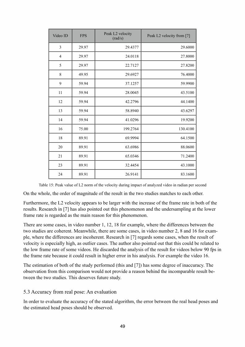
Video ID FPS Peak L2 velocity(rad/s) Peak L2 velocity from [7]
3 29.97 29.4377 29.6000
4 29.97 24.0118 27.8000
5 29.97 22.7127 27.8200
8 49.95 29.6927 76.4000
9 59.94 37.1257 59.9900
11 59.94 28.0045 43.5100
12 59.94 42.2796 44.1400
13 59.94 58.8940 43.6297
14 59.94 41.0296 19.9200
16 75.00 199.2764 130.4100
18 89.91 69.9994 64.1500
20 89.91 63.6986 88.0600
21 89.91 65.0346 71.2400
23 89.91 32.4454 43.1000
24 89.91 26.9141 83.1600
Table 15: Peak value of L2 norm of the velocity during impact of analyzed video in radian per second
On the whole, the order of magnitude of the result in the two studies matches to each other.
Furthermore, the L2 velocity appears to be larger with the increase of the frame rate in both of the results. Research in [7] has also pointed out this phenomenon and the undersampling at the lower frame rate is regarded as the main reason for this phenomenon.
There are some cases, in video number 1, 12, 18 for example, where the differences between the two studies are coherent. Meanwhile, there are some cases, in video number 2, 8 and 16 for exam-ple, where the differences are incoherent. Research in [7] regards some cases, when the result of velocity is especially high, as outlier cases. The author also pointed out that this could be related to the low frame rate of some videos. He discarded the analysis of the result for videos below 90 fps in the frame rate because it could result in higher error in his analysis. For example the video 16.
The estimation of both of the study performed (this and [7]) has some degree of inaccuracy. The observation from this comparison would not provide a reason behind the incomparable result be-tween the two studies. This deserves future study.
5.3 Accuracy from real pose: An evaluation
In order to evaluate the accuracy of the stated algorithm, the error between the real head poses and the estimated head poses should be observed.
49

The real head poses database used in this project are obtained from the result of [20]. This database contains 2790 monocular face image of 15 persons. One of them is used to evaluate the Posit algo-rithm in this project.
According to the Euler angle definitions in this project, the database contains the head poses with the tilt/roll angles ranges in:
0 15 30 60 90 270 300 330 345 in degrees
it contains pan/pitch angles ranges in:
-90 -75 -60 -45 -30 -15 0 15 30 45 60 75 90 in degrees
and it contains the single roll value of:
0, in degrees [delimitation 5.2]
The singleton of the roll value means the head is not rotating in the z-axis in the database.
There are totally 93 face pictures for a single person.
The error of the head poses is calculated using the difference of the real head pose values and the estimated head pose values, so,
error(roll) = estimated head pose roll - real head pose roll
error(pitch) = estimated head pose pitch - real head pose pitch
error(yaw) = estimated head pose yaw - real head pose yaw
The head model used for evaluation is created using method in Appendix II. The focal length is measured using method in Appendix I utilizing the created head model.
The result of the estimation errors for the head poses can be illustrated in the following table:
R Roll R Pitch R Yaw P Roll P Pitch P Yaw E Roll E Pitch E Yaw
90 0 0 65.84 5.21 3.37 -24.16 5.21 3.37
60 90 0 52.94 64.37 17.41 -7.06 -25.63 17.41
60 75 0 46.83 61.20 7.11 -13.17 -13.80 7.11
60 60 0 42.40 50.17 -2.48 -17.60 -9.83 -2.48
60 45 0 49.10 33.14 0.78 -10.90 -11.86 0.78
60 30 0 44.53 21.41 -4.73 -15.47 -8.59 -4.73
60 15 0 41.82 8.78 -5.82 -18.18 -6.22 -5.82
60 0 0 44.75 -2.25 -2.55 -15.25 -2.25 -2.55
60 -15 0 45.98 2.23 -4.95 -14.02 17.23 -4.95
50
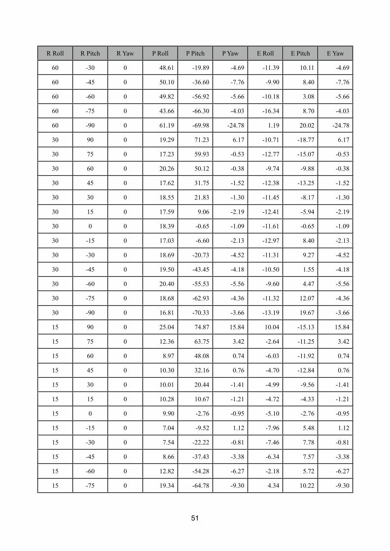
R Roll R Pitch R Yaw P Roll P Pitch P Yaw E Roll E Pitch E Yaw
60 -30 0 48.61 -19.89 -4.69 -11.39 10.11 -4.69
60 -45 0 50.10 -36.60 -7.76 -9.90 8.40 -7.76
60 -60 0 49.82 -56.92 -5.66 -10.18 3.08 -5.66
60 -75 0 43.66 -66.30 -4.03 -16.34 8.70 -4.03
60 -90 0 61.19 -69.98 -24.78 1.19 20.02 -24.78
30 90 0 19.29 71.23 6.17 -10.71 -18.77 6.17
30 75 0 17.23 59.93 -0.53 -12.77 -15.07 -0.53
30 60 0 20.26 50.12 -0.38 -9.74 -9.88 -0.38
30 45 0 17.62 31.75 -1.52 -12.38 -13.25 -1.52
30 30 0 18.55 21.83 -1.30 -11.45 -8.17 -1.30
30 15 0 17.59 9.06 -2.19 -12.41 -5.94 -2.19
30 0 0 18.39 -0.65 -1.09 -11.61 -0.65 -1.09
30 -15 0 17.03 -6.60 -2.13 -12.97 8.40 -2.13
30 -30 0 18.69 -20.73 -4.52 -11.31 9.27 -4.52
30 -45 0 19.50 -43.45 -4.18 -10.50 1.55 -4.18
30 -60 0 20.40 -55.53 -5.56 -9.60 4.47 -5.56
30 -75 0 18.68 -62.93 -4.36 -11.32 12.07 -4.36
30 -90 0 16.81 -70.33 -3.66 -13.19 19.67 -3.66
15 90 0 25.04 74.87 15.84 10.04 -15.13 15.84
15 75 0 12.36 63.75 3.42 -2.64 -11.25 3.42
15 60 0 8.97 48.08 0.74 -6.03 -11.92 0.74
15 45 0 10.30 32.16 0.76 -4.70 -12.84 0.76
15 30 0 10.01 20.44 -1.41 -4.99 -9.56 -1.41
15 15 0 10.28 10.67 -1.21 -4.72 -4.33 -1.21
15 0 0 9.90 -2.76 -0.95 -5.10 -2.76 -0.95
15 -15 0 7.04 -9.52 1.12 -7.96 5.48 1.12
15 -30 0 7.54 -22.22 -0.81 -7.46 7.78 -0.81
15 -45 0 8.66 -37.43 -3.38 -6.34 7.57 -3.38
15 -60 0 12.82 -54.28 -6.27 -2.18 5.72 -6.27
15 -75 0 19.34 -64.78 -9.30 4.34 10.22 -9.30
51
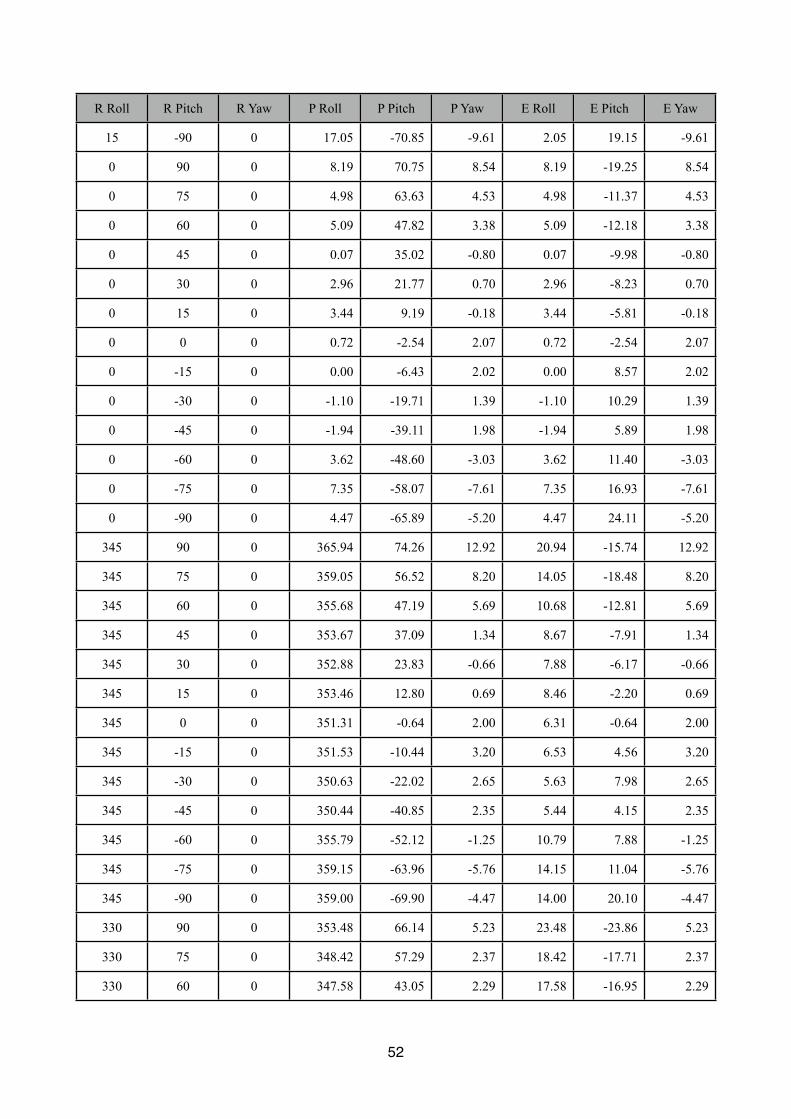
R Roll R Pitch R Yaw P Roll P Pitch P Yaw E Roll E Pitch E Yaw
15 -90 0 17.05 -70.85 -9.61 2.05 19.15 -9.61
0 90 0 8.19 70.75 8.54 8.19 -19.25 8.54
0 75 0 4.98 63.63 4.53 4.98 -11.37 4.53
0 60 0 5.09 47.82 3.38 5.09 -12.18 3.38
0 45 0 0.07 35.02 -0.80 0.07 -9.98 -0.80
0 30 0 2.96 21.77 0.70 2.96 -8.23 0.70
0 15 0 3.44 9.19 -0.18 3.44 -5.81 -0.18
0 0 0 0.72 -2.54 2.07 0.72 -2.54 2.07
0 -15 0 0.00 -6.43 2.02 0.00 8.57 2.02
0 -30 0 -1.10 -19.71 1.39 -1.10 10.29 1.39
0 -45 0 -1.94 -39.11 1.98 -1.94 5.89 1.98
0 -60 0 3.62 -48.60 -3.03 3.62 11.40 -3.03
0 -75 0 7.35 -58.07 -7.61 7.35 16.93 -7.61
0 -90 0 4.47 -65.89 -5.20 4.47 24.11 -5.20
345 90 0 365.94 74.26 12.92 20.94 -15.74 12.92
345 75 0 359.05 56.52 8.20 14.05 -18.48 8.20
345 60 0 355.68 47.19 5.69 10.68 -12.81 5.69
345 45 0 353.67 37.09 1.34 8.67 -7.91 1.34
345 30 0 352.88 23.83 -0.66 7.88 -6.17 -0.66
345 15 0 353.46 12.80 0.69 8.46 -2.20 0.69
345 0 0 351.31 -0.64 2.00 6.31 -0.64 2.00
345 -15 0 351.53 -10.44 3.20 6.53 4.56 3.20
345 -30 0 350.63 -22.02 2.65 5.63 7.98 2.65
345 -45 0 350.44 -40.85 2.35 5.44 4.15 2.35
345 -60 0 355.79 -52.12 -1.25 10.79 7.88 -1.25
345 -75 0 359.15 -63.96 -5.76 14.15 11.04 -5.76
345 -90 0 359.00 -69.90 -4.47 14.00 20.10 -4.47
330 90 0 353.48 66.14 5.23 23.48 -23.86 5.23
330 75 0 348.42 57.29 2.37 18.42 -17.71 2.37
330 60 0 347.58 43.05 2.29 17.58 -16.95 2.29
52
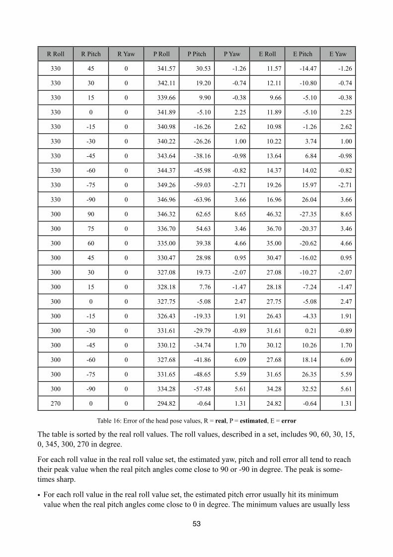
R Roll R Pitch R Yaw P Roll P Pitch P Yaw E Roll E Pitch E Yaw
330 45 0 341.57 30.53 -1.26 11.57 -14.47 -1.26
330 30 0 342.11 19.20 -0.74 12.11 -10.80 -0.74
330 15 0 339.66 9.90 -0.38 9.66 -5.10 -0.38
330 0 0 341.89 -5.10 2.25 11.89 -5.10 2.25
330 -15 0 340.98 -16.26 2.62 10.98 -1.26 2.62
330 -30 0 340.22 -26.26 1.00 10.22 3.74 1.00
330 -45 0 343.64 -38.16 -0.98 13.64 6.84 -0.98
330 -60 0 344.37 -45.98 -0.82 14.37 14.02 -0.82
330 -75 0 349.26 -59.03 -2.71 19.26 15.97 -2.71
330 -90 0 346.96 -63.96 3.66 16.96 26.04 3.66
300 90 0 346.32 62.65 8.65 46.32 -27.35 8.65
300 75 0 336.70 54.63 3.46 36.70 -20.37 3.46
300 60 0 335.00 39.38 4.66 35.00 -20.62 4.66
300 45 0 330.47 28.98 0.95 30.47 -16.02 0.95
300 30 0 327.08 19.73 -2.07 27.08 -10.27 -2.07
300 15 0 328.18 7.76 -1.47 28.18 -7.24 -1.47
300 0 0 327.75 -5.08 2.47 27.75 -5.08 2.47
300 -15 0 326.43 -19.33 1.91 26.43 -4.33 1.91
300 -30 0 331.61 -29.79 -0.89 31.61 0.21 -0.89
300 -45 0 330.12 -34.74 1.70 30.12 10.26 1.70
300 -60 0 327.68 -41.86 6.09 27.68 18.14 6.09
300 -75 0 331.65 -48.65 5.59 31.65 26.35 5.59
300 -90 0 334.28 -57.48 5.61 34.28 32.52 5.61
270 0 0 294.82 -0.64 1.31 24.82 -0.64 1.31
Table 16: Error of the head pose values, R = real, P = estimated, E = error
The table is sorted by the real roll values. The roll values, described in a set, includes 90, 60, 30, 15, 0, 345, 300, 270 in degree.
For each roll value in the real roll value set, the estimated yaw, pitch and roll error all tend to reach their peak value when the real pitch angles come close to 90 or -90 in degree. The peak is some-times sharp.
• For each roll value in the real roll value set, the estimated pitch error usually hit its minimum value when the real pitch angles come close to 0 in degree. The minimum values are usually less
53

than 10 degrees. The error is small(<5) when the real pitch values lays between -30 to 30 in de-gree and medium(<10) between -45 to 45 in degree.
• For each roll value in the real roll value set, the estimated error for the roll angles tends to fluctu-ate around a value. The value is large (>15) when the real roll values are among 90, 60, 300, and 270 in degree, medium (10-15) when they are among 30 and 330 in degree and small (<10) when they are among 0, 15, 345 in degree.
• For each of the roll value set, the estimated yaw error is normally smaller than 5 degrees except only in some cases when the real pitch values come close to -90 or 90 in degree.
After overall consideration, the important result that could be reflected in the evaluation is that the head pose estimation in Motiontracker would result in:
• Good estimation when the real roll value of the head relative to the camera lays between -15 to 15 in degree and when the real pitch value of the head relative to the camera lays between -30 to 30 in degree when both of them are converted to the sequential domain
• Acceptable estimation when the real roll value of the head relative to the camera lays between -30 to 30 in degree and when the real pitch value of the head relative to the camera lays between -45 to 45 in degree when both of them are converted to sequential domain
• Unacceptable estimation in other domains
The words such as good and acceptable are mainly served as a recommendation of the usage sce-nario of MotionTracker.
From the information we could obtain, the sources of errors could be:
• The input of Posit algorithm. Namely the error in the M array, I array and focal length assignment. We have done most part in this project to make it more accurate.
• The gimbal lock effect, where the accuracy of Euler angle inevitably suffers from[19]. The evalua-tion part demonstrates that there are comparatively larger error of estimation when the real roll and pitch angle are large. This is a phenomenon that will result in when the gimbal lock are taking effect.
• It could be related to the person’s real pose errors in the database itself.
• The inaccuracy from Posit algorithm
5.4 Summary of requirements and applicability of the method
The summary of requirements and applicability of the method becomes clear and suitable for dis-cussion after we have done the evaluation in the previous section.
Summary of Requirements for analysis
Firstly, the set of tools should be prepared for the analysis.
• MotionTracker
• VirtualDub
54

• DivX
• AviSynth
Research Material
• We need to obtain a video containing head object and head motion
• Make sure that the internal depth of the head object is so small compared to its distance from the camera
To perform the Posit algorithm
• We need to provide with the estimated focal length or a focal length which is large enough so that its value has a tiny impact on the output head pose values
• We need to provide with the head model of the person in the video
• We need to provide with the image points of the person in the video
To estimate the focal length(See Appendix I)
• We need to know the estimated real distance from the head object to the camera
• We need to know the front view of the head object of the analysed person
• We need to know the head model of the head object of the analysed person
To create head model(See Appendix II)
• We need to obtain the front view of the head object of the analysed or sample person
• We need to obtain the side view of the head object of the analysed or sample person
• We need to provide with a head breadth of the aforementioned head object
To create image points
• The model keys for each image in the image sequence are expected to be fully recognized either using template method or done manually. If some of the model keys cannot be recognized, the image is considered a failure to provide useful information.
• The failure rate is expected to be lower than 10%
Applicability of the analysis
To create good result in a single image, we have to make sure that the real roll and pitch value of the analysed head object are constrained in:
Real roll valuesReal roll values Real pitch valueReal pitch value
> -15 > -30
< 15 < 30
To create acceptable result in a single image, we have to make sure that the real roll and pitch value of the analysed head object are constrained in:
55

Real roll valuesReal roll values Real pitch valueReal pitch value
> -30 > -45
< 30 < 45
The applicability is examined by the inspection of the image in the image sequence. Expertise in the estimation of human pose value from images using other tools is required to make sure that the above thresholds are maintained.
These skills could involve the understanding of relative position of different feature points on the head object. They deserve future study and research.
56
6 Delimitation and conclusionIn this section, the delimitation and the summary of the project will be discussed. The delimitation part is labeled in the pattern of X.Y, which means it is the Y-th delimitation in Chapter X.
6.1 Delimitation
Delimitation 3.1
The head model used in the project is simplified to the left ear model or the right ear model with only 4 points needed to find the head pose values we need. It is not surprise to find noticeable val-ues in the error measurement in some cases because of the very simplified model.
It is not easy for human being to pick up the feature points in the low resolution images, so we can only rely on some dominant features such as the eye position and nose position for easier operation. The manually picked up image points also raised inaccuracy issue of the algorithm although some measures has been taken to speed up the selection of points. The method to overcome this issue is not addressed in this project.
Furthermore, we have to point out that the model used for boxing match analysis is created using the sample person in [20], not the actual boxer. It is practically difficult to find the head model for the boxer unless we have high resolution of the boxer’s head images.
Delimitation 3.2
In this project, a fixed focal length is used for the Posit algorithm for the analysis of the boxing matches. The reasons we are not able to carry out the focal length measurement in Appendix I for the boxing match analysis includes:
• The distance between the boxer and the camera is not known. Although there are documents[22]
says a standard boxing ring is between 4.9 and 7.6 m to a side between the ropes, the clue is not strong enough for the determination of the actual distance
• It is hard to find the front view of the face as required by the process introduced in Appendix I. Even if we did found, the face tends to be too small for the accurate calculation of Tz
However, the focal length should not be taken great concern since the nature of Posit algorithm pro-duces stable head pose value and instable head distance value regardless of focal length chosen as long as the object is far away from the camera. This fact is obtained by the observation in Appendix I which can be summarized as:
When the focal length are large enough, the variation of it would have little impact on the head pose values and Tx, Ty component of the head distance values.
Delimitation 4.1
When we are using the left ear model, we made the assumption that the left ear is visible to the ob-server for the pick up of the image points. This is not always true because the feature points could be occluded sometimes although the left ear model is apparently better than the right ear model anyway.
The effect of the occluded points is discussed in Section 4.3.
57
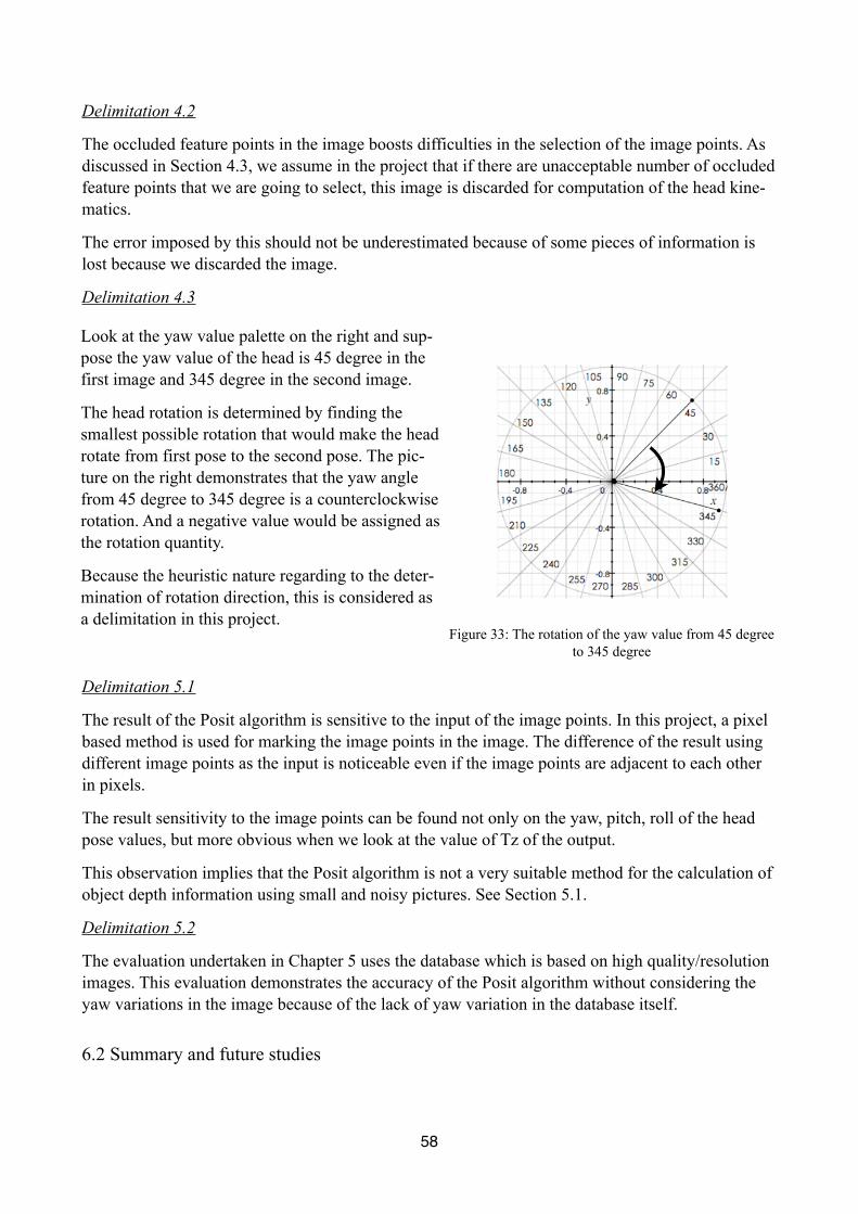
Delimitation 4.2
The occluded feature points in the image boosts difficulties in the selection of the image points. As discussed in Section 4.3, we assume in the project that if there are unacceptable number of occluded feature points that we are going to select, this image is discarded for computation of the head kine-matics.
The error imposed by this should not be underestimated because of some pieces of information is lost because we discarded the image.
Delimitation 4.3
Delimitation 5.1
The result of the Posit algorithm is sensitive to the input of the image points. In this project, a pixel based method is used for marking the image points in the image. The difference of the result using different image points as the input is noticeable even if the image points are adjacent to each other in pixels.
The result sensitivity to the image points can be found not only on the yaw, pitch, roll of the head pose values, but more obvious when we look at the value of Tz of the output.
This observation implies that the Posit algorithm is not a very suitable method for the calculation of object depth information using small and noisy pictures. See Section 5.1.
Delimitation 5.2
The evaluation undertaken in Chapter 5 uses the database which is based on high quality/resolution images. This evaluation demonstrates the accuracy of the Posit algorithm without considering the yaw variations in the image because of the lack of yaw variation in the database itself.
6.2 Summary and future studies
Look at the yaw value palette on the right and sup-pose the yaw value of the head is 45 degree in the first image and 345 degree in the second image.
The head rotation is determined by finding the smallest possible rotation that would make the head rotate from first pose to the second pose. The pic-ture on the right demonstrates that the yaw angle from 45 degree to 345 degree is a counterclockwise rotation. And a negative value would be assigned as the rotation quantity.
Because the heuristic nature regarding to the deter-mination of rotation direction, this is considered as a delimitation in this project.
Figure 33: The rotation of the yaw value from 45 degree to 345 degree
58
In this study, a computer program is developed to extract the head kinematic information from a set of boxing match videos. Specifically speaking, the head distance values and head pose values of the struck boxers’ head are obtained with the model points and image points assigned.
The database, which contains 25 videos of knock-out boxing matches, are analyzed. Methods of the preprocessing of the videos using progressive scan video deinterlacing technique are carried out to make the research material more suitable for video analysis.
In this project, the Posit algorithm are used to extract the head motion information from these vid-eos. Various techniques are used to prepare for the input of the Posit algorithm, namely, the image points, the model points and the focal length.
A motion analysis software is created to load the created image points and model points into the software automatically. The Posit algorithm can be carried out in this software and the output can be represented in the logger of the software for further analysis and evaluation.
The simplified model creation and automatic feature point matching makes the selection of image points easier. Normally it would take less than five minutes to make one video clip ready for motion analysis.
In order to smooth the data representation, the interpolation of the velocity data is undertaken in Matlab. This process also enable us to produce useful peak velocity values that can be used to make comparison with the same quantity in the related studies.
In this study, compared to the project[7] which it is based on, there are several minor improvement, it:
• Made the selection of image points easier by template method in image processing
• Performed the video deinterlacing using VirtualDub
• Made the angular velocity be represented alone 3 separate axis when taking advantage of the Posit algorithm
• Shows a evaluation that identified the accuracy of this method
The comparable result of the study in this project in shown in Table 14. The table demonstrates that there are cases when the result in this paper is coherent with the one it is based on[7]. However, there are also cases when unstable and large variations of the result do exist between the studies.
The piece of information that revealed in the evaluation section of this paper appears to be a nice verification of the property of Euler angle. The error of MotionTracker can be assumed to have a larger error estimation when the real pitch or roll value of the sample person is greater than a certain limit.
In this study, we have not focused on finding out the reason behind the difference of results between the two studies. However, this also means the comparison of these two reports could be an interest-ing area in the future study.
This study is expected to be extensible by supplying different research materials into the Motion-tracker.
59

To put it together, this study created an effective way to obtain the head kinematic information us-ing OpenCV library under Macintosh platform. The order of magnitude of some of the result in this study is comparable with the related study which this project is based on. When carrying out the motion study applying the software in this project, the researcher should be aware of the property of the Euler angle which is demonstrated in the evaluation part of this paper.
60
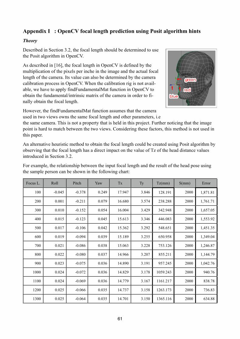
Appendix I : OpenCV focal length prediction using Posit algorithm hintsTheory
Described in Section 3.2, the focal length should be determined to use the Posit algorithm in OpenCV.
As described in [16], the focal length in OpenCV is defined by the multiplication of the pixels per inche in the image and the actual focal length of the camera. Its value can also be determined by the camera calibration process in OpenCV. When the calibration rig is not avail-able, we have to apply findFundamentalMat function in OpenCV to obtain the fundamental/intrinsic matrix of the camera in order to fi-nally obtain the focal length.
However, the findFundamentalMat function assumes that the camera used in two views owns the same focal length and other parameters, i.e the same camera. This is not a property that is held in this project. Further noticing that the image point is hard to match between the two views. Considering these factors, this method is not used in this paper.
An alternative heuristic method to obtain the focal length could be created using Posit algorithm by observing that the focal length has a direct impact on the value of Tz of the head distance values introduced in Section 3.2.
For example, the relationship between the input focal length and the result of the head pose using the sample person can be shown in the following chart:
Focus L. Roll Pitch Yaw Tx Ty Tz(mm) S(mm) Error
100 -0.045 -0.378 0.249 17.947 3.846 128.191 2000 1,871.81
200 0.001 -0.211 0.079 16.680 3.574 238.288 2000 1,761.71
300 0.010 -0.152 0.054 16.004 3.429 342.948 2000 1,657.05
400 0.015 -0.123 0.045 15.613 3.346 446.083 2000 1,553.92
500 0.017 -0.106 0.042 15.362 3.292 548.651 2000 1,451.35
600 0.019 -0.094 0.039 15.189 3.255 650.958 2000 1,349.04
700 0.021 -0.086 0.038 15.063 3.228 753.126 2000 1,246.87
800 0.022 -0.080 0.037 14.966 3.207 855.211 2000 1,144.79
900 0.023 -0.075 0.036 14.890 3.191 957.245 2000 1,042.76
1000 0.024 -0.072 0.036 14.829 3.178 1059.243 2000 940.76
1100 0.024 -0.069 0.036 14.779 3.167 1161.217 2000 838.78
1200 0.025 -0.066 0.035 14.737 3.158 1263.173 2000 736.83
1300 0.025 -0.064 0.035 14.701 3.150 1365.116 2000 634.88
��������
������
����������
61
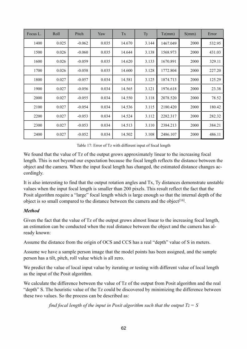
Focus L. Roll Pitch Yaw Tx Ty Tz(mm) S(mm) Error
1400 0.025 -0.062 0.035 14.670 3.144 1467.049 2000 532.95
1500 0.026 -0.060 0.035 14.644 3.138 1568.973 2000 431.03
1600 0.026 -0.059 0.035 14.620 3.133 1670.891 2000 329.11
1700 0.026 -0.058 0.035 14.600 3.128 1772.804 2000 227.20
1800 0.027 -0.057 0.034 14.581 3.125 1874.713 2000 125.29
1900 0.027 -0.056 0.034 14.565 3.121 1976.618 2000 23.38
2000 0.027 -0.055 0.034 14.550 3.118 2078.520 2000 78.52
2100 0.027 -0.054 0.034 14.536 3.115 2180.420 2000 180.42
2200 0.027 -0.053 0.034 14.524 3.112 2282.317 2000 282.32
2300 0.027 -0.053 0.034 14.513 3.110 2384.213 2000 384.21
2400 0.027 -0.052 0.034 14.502 3.108 2486.107 2000 486.11
Table 17: Error of Tz with different input of focal length
We found that the value of Tz of the output grows approximately linear to the increasing focal length. This is not beyond our expectation because the focal length reflects the distance between the object and the camera. When the input focal length has changed, the estimated distance changes ac-cordingly.
It is also interesting to find that the output rotation angles and Tx, Ty distances demonstrate unstable values when the input focal length is smaller than 200 pixels. This result reflect the fact that the Posit algorithm require a “large” focal length which is large enough so that the internal depth of the object is so small compared to the distance between the camera and the object[16].
Method
Given the fact that the value of Tz of the output grows almost linear to the increasing focal length, an estimation can be conducted when the real distance between the object and the camera has al-ready known:
Assume the distance from the origin of OCS and CCS has a real “depth” value of S in meters.
Assume we have a sample person image that the model points has been assigned, and the sample person has a tilt, pitch, roll value which is all zero.
We predict the value of local input value by iterating or testing with different value of local length as the input of the Posit algorithm.
We calculate the difference between the value of Tz of the output from Posit algorithm and the real “depth” S. The heuristic value of the Tz could be discovered by minimizing the difference between these two values. So the process can be described as:
find focal length of the input in Posit algorithm such that the output Tz = S
62

According to the table for example, 1900mm would be an good value for focal length because the error would bottom out at that point.
63

Appendix II : The creation of the simplified head model using MotionTrackerTheory
The model points that are going to be arranged in the OCS has the pattern shown in Figure 11. We would like to assign the blue axis as the z-axis, red axis as the x-axis and green axis as the y-axis. In the front view of the head model, the XOY plane is shown and the z-axis is occluded from the viewer; in the side view of the head model, the YOZ plane is shown and the x-axis is occluded from the viewer.
Given the model keys in the M array, the creation of the simplified head model involves finding the coordinate values of these model keys.
Method
The predefined model keys, as described in Section 3.3, can be listed as: Nose, Left Eye, Right Eye, Left Ear and the Right Ear in order.
To obtain the model point coordinates, we first try to load the front view of the sample person:
Figure 34: Front View of the sample person is selected with the image points that is used to construct the head model
The front view of the head is defined as the head image which has the head pose values all equal to zero with respect to the camera. The front view of the head tells us about the x and y coordinates of the internal structure of the head. If we pick up the points on the front view of the head with respect to the model keys, the x and y coordinates of the model keys can be calculated and obtained.
In this project, we regard the sample person’s head as symmetric, which means we only have to pick up half of the points on the front view of the head to create the entire head model. Namely the nose, left eye and the left ear.
In the above picture for example, the front view of the head is loaded on the left hand side. We pick up the model points in the image plane with respect to the model keys in order. When that is done, we would see the picture on the right hand side. The marked “0” on the picture represents the nose point, “1” represents the left eye, “2” represents the left ear.
In order to better represent the head structure, the nose point is selected to be located at the origin of OCS. We shift all the points in the model so that the nose point has the coordinate value (0, 0).
Furthermore, since the model points is initially unit-less, the value of the model point coordinates should be scaled to the unit of millimeters. In this paper, the left ear and the right ear is assumed to
64
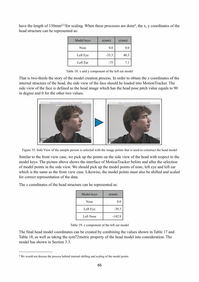
have the length of 150mm[21]for scaling. When these processes are done4, the x, y coordinates of the head structure can be represented as:
Model keys x(mm) y(mm)
Nose 0.0 0.0
Left Eye -33.3 40.5
Left Ear -75 7.1
Table 18: x and y component of the left ear model
That is two-thirds the story of the model creation process. In order to obtain the z coordinates of the internal structure of the head, the side view of the face should be loaded into MotionTracker. The side view of the face is defined as the head image which has the head pose pitch value equals to 90 in degree and 0 for the other two values.
Figure 35: Side View of the sample person is selected with the image points that is used to construct the head model
Similar to the front view case, we pick up the points on the side view of the head with respect to the model keys. The picture above shows the interface of MotionTracker before and after the selection of model points in the side view. We should pick up the model points of nose, left eye and left ear which is the same as the front view case. Likewise, the model points must also be shifted and scaled for correct representation of the data.
The z coordinates of the head structure can be represented as:
Model keys z(mm)
Nose 0.0
Left Eye -39.3
Left Nose -142.9
Table 19: z component of the left ear model
The final head model coordinates can be created by combining the values shown in Table 17 and Table 18, as well as taking the sym72metric property of the head model into consideration. The model has shown in Section 3.3.
65
4 We would not discuss the process behind internal shifting and scaling of the model points

Appendix III : MotionTracker User ManualMotionTracker manual is the place where the instruction is given on how to use this software. This manual is the excerpt from the MotionTracker help information.
• How to load a sequence of image into Motiontracker
Motiontracker enables you to load a set of images for motion analysis. The folder that contains the set of images you want to analyze is called the image folder. The image folder could contain the fol-lowing content:
• (Required) PNG format image sequence labeled as: AAAA_BBBB. AAAA identify the con-tents of the image sequence. BBBB defines the order of the image sequence
• (Optional) Created from Motiontracker, the image point list for each of the image in the im-age sequence
• (Optional) The plist file containing the model of the object for analysis in the image se-quence. This is required if you need to perform motion analysis
1. Open Motiontracker if it is not2. Open Finder3. In Finder, find the image folder you want to perform motion analysis4. Drag the image folder to the Motiontracker panel. It is easier to do so when the Finder and
Motiontracker is both visible
• How to create simplified object model for motion analysis
Motiontracker enables motion analyzer to create two specific model for the human head. You are required only to provide with two images of the analyzed person's head of particular view angles, mark the key points of the models and Motiontracker would create the model plist file for you.
The two models are called the right ear model and the left ear model. The key for the models are:
Right ear model keys
Nose
Left Eye
Right Eye
Right Ear
and
Left ear model keys
Nose
Left Eye
Right Eye
66

Left Ear
To create right ear model,
1. Prepare for the image folder. The image folder should contain images of:a. Front view of the analyzed person's headb. Right side view of the analyzed person's head
2. Make sure that the file containing the front view of the person is named alphabetically in front of the side view picture. For example, 0.png stands for the front view and 1.png stands for the side view
3. Load image folder into Motiontracker4. Mark right ear model keys for the front view and side view of the analyzed person5. Assign in the panel, the head breadth of the person, for example 150 millimeter6. Click the "Create Right Ear Model" button. The model plist file is then created inside the image
folder with the name "NewRightEar.plist"To create left ear model,
1. Prepare for the image folder. The image folder should contain images of:◦ Front view of the analyzed person's head◦ Left side view of the analyzed person's head
2. Make sure that the file containing the front view of the person is named alphabetically in front of the side view picture. For example, 0.png stands for the front view and 1.png stands for the side view
3. Load image folder into Motiontracker4. Mark left ear model keys for the front view and side view of the analyzed person5. Assign in the panel, the head breadth of the person, for example 150 millimeter6. Click the "Create Left Ear Model" button. The model plist file is then created inside the im-
age folder with the name "NewLeftEar.plist"
• How to mark feature points in the image sequence
Motiontracker makes it intuitive to mark feature point in the image manually. The feature point can be automatically saved into the file system in a one-to-one bases, which means there is one feature point record for every image in the image sequence. When the image is loaded, the feature point record is reloaded and ready for use in the software.
To mark the feature point,
1. Open Motiontracker if it is not2. Load image folder. The image viewer is shown when the image is loaded.3. Use mouse wheel or the image slider in the Motiontracker panel. Traverse to the image
whose feature points need to be marked out4. When the mouse is hovering over the image view, the cursor would turn into a image
marker. With the cursor in this state, mark the keys sequentially according to the order of model keys in the plist file. This process can be decomposed into:
• Move the mouse into the first key in the model, hold ⌥ key and click the mouse• Move the mouse to the second key in the model, do the same mouse clicking as before
67
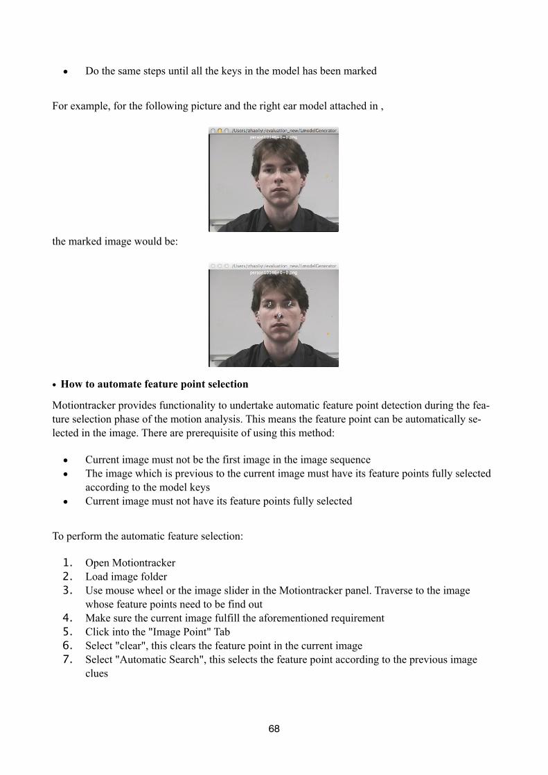
• Do the same steps until all the keys in the model has been marked
For example, for the following picture and the right ear model attached in ,
the marked image would be:
• How to automate feature point selection
Motiontracker provides functionality to undertake automatic feature point detection during the fea-ture selection phase of the motion analysis. This means the feature point can be automatically se-lected in the image. There are prerequisite of using this method:
• Current image must not be the first image in the image sequence• The image which is previous to the current image must have its feature points fully selected
according to the model keys• Current image must not have its feature points fully selected
To perform the automatic feature selection:
1. Open Motiontracker2. Load image folder3. Use mouse wheel or the image slider in the Motiontracker panel. Traverse to the image
whose feature points need to be find out4. Make sure the current image fulfill the aforementioned requirement5. Click into the "Image Point" Tab6. Select "clear", this clears the feature point in the current image7. Select "Automatic Search", this selects the feature point according to the previous image
clues
68

When the result of automatic feature selection is not satisfactory, feature points still need to be edited in a manual fashion after the automatic feature point selection.
• How to estimate focal length of the camera
There are several ways to provide the focal length information for the motion analysis in Motion-tracker:
• The focal length has already known for use in the OpenCV posit function• A focal length which is large enough so that it has a tiny impact on the result. A reference
value is 2000 pixels• Make an estimation of the focal length using the following procedure
1. Prepare for the image folder. The image folder should contain the content of:◦ Front view of the analyzed object◦ Model plist file of the analyzed object
2. Load image folder into Motiontracker3. Mark model keys according to the model plist file for the front view of the analyzed object4. Assign in the panel, the supposed distance from the viewer to the analyzed object5. Click the "Estimate Posit Focal Length" button, the estimated focal length is shown in the
focal length text input box in the panel.
• How to undertake motion analysis in Motiontracker
Motiontracker is a motion analysis tool. The process of the motion analysis could contain the fol-lowing steps.
To perform motion analysis in Motiontracker:
1. Open Motiontracker if it is not2. Load image folder3. Click the "Image Point" tab, mark feature point for every image in the image sequence4. Click the "Posit" tab, assign frame rate of the image sequence5. In the "Posit" tab, assign focal length of the camera6. Click "Generate pose" to get the result
It is very important to get the frame rate right in the procedure because it affects the order of magnitude of the result
• How to edit feature points in Motiontracker
Feature points, which is loaded from the feature point files in the image folder, or marked in the Motiontracker either automatically or manually, are editable in Motiontracker.
To edit feature points,
69

1. Open Motiontracker2. Load image folder3. Use mouse wheel or the image slider in the Motiontracker panel. Traverse to the image
whose feature points need to be edited4. Click into the "Image Point" Tab
After that you might perform the following operations:
To clear all the feature point in the current image
1. Hold ⌥(Option) Key and click the mouse in the image viewerTo translate all the feature point in the current image
1. Click and hold the right mouse key, drag the mouseTo edit the position of a single feature point in the current image
1. Click the point you want to edit, the point turns red after it is selected. You can perform one of the following operations:◦ Using arrow keys to move the selected feature point◦ Using mouse dragging to move the selected feature points
To edit the position of multiple feature points in the current image
1. Hold ^(Control) Key and click the points you want to edit, the points turn red after it is se-lected. Re-click the point to deselect it. You can perform one of the following operations:◦ Using arrow keys to move the selected feature point◦ Using mouse dragging to move the selected feature points
• How to perform basic image processing operation in Motiontracker
You can perform some basic image processing operations in Motiontracker.
1. Open Motiontracker2. Load image folder3. Use mouse wheel or the image slider in the Motiontracker panel. Traverse to the image
which needs to perform image processingAfter that you might perform the following operations:
To perform image thresholding
1. Click "Thresholding" Tab2. Make selection of different options and see result in the image viewer3. Click "Show Threshold image" button and see result in the image viewer
To perform image smoothing
1. Click "Blurring" Tab2. Make selection of different options and see result in the image viewer
70

3. Click "Show Blurred image" button and see result in the image viewerTo perform image morphology
1. Click "Morphology" Tab2. Make selection of different options and see result in the image viewer3. Click "Show Morphological image" button and see result in the image viewer
To obtain contours and lines in the image
1. Click "Contours" Tab2. Make selection of different options and see result in the image viewer3. Click "Show Hough Line" or "Show Contours" button and see result in the image viewer
Make sure the function is activated by clicking the check box beside the button.
71
References[1] World Health Organization, Annex Table 2: Deaths by cause, sex and mortality stratum in WHO re-
gions estimates for 2002, The world health report, 2004[2] Andrew IR Maas, Nino Stocchetti, MDb, Ross Bullock, Moderate and severe traumatic brain injury
in adults, Volume 7, Issue 8, 2008, pp. 728–741[3] Simon R. Finfer, Jeremy Cohen, Severe traumatic brain injury, Resuscitation, Volume 48, Issue 1,
2001, pp. 77–90[4] Department of Defense and Department of Veterans Affairs, Traumatic Brain Injury Task Force,
http://www.cdc.gov/nchs/data/icd9/Sep08TBI.pdf, 2008[5] J Ghajar, Traumatic brain injury, Lancet Issue 356, 2000, pp. 923–929[6] Yi Ma, Stefano Soatto, Jana Kosecka, Shankar S.Sastry, An Invitation to 3-D Vision, Chapter 1,
Springer, 2004[7] Enrico Pellegrini, Kinematic evaluation of traumatic brain injuries in boxing, 2011 [8] Daniel F. DeMenthon, Larry S. Davis, Model-Based Object Pose in 25 Lines of Code, Computer Vi-
sion Laboratory, University of Maryland[9] Fischler, M.A., and R.C. Bolles, Random Sample Consensus: A Paradigm for model fitting applica-
tions to Image Analysis and Automated Cartography, Comm/ ACM, vol.24, 1981, pp. 381-395[10] R. Brunelli, Template Matching Techniques in Computer Vision: Theory and Practice, Wiley, ISBN
978-0-470-51706-2, 2009 [11] Roy, Quick and easy head pose estimation with OpenCV,
http://www.morethantechnical.com/2010/03/19/quick-and-easy-head-pose-estimation-with-opencv-w-code
[12] 100fps, What is Deinterlacing? Facts, solutions, examples, http://www.100fps.com[13] Gunnar Thalin, Deinterlace - smooth, http://www.guthspot.se/video/#deinterlacesmooth[14] S. Suzuki and K. Abe, Topological structural analysis of digital binary images by border following,
Computer Vision, Graphics and Image Processing 30, 1985, pp. 32-46[15] Wikipedia, Rigid body, http://en.wikipedia.org/wiki/Rigid_body[16] Gary Bradski, Adrian Kaehler, Learning OpenCV, Chapter 12, O'Relly, ISBN 978-7-302-20993-5,
2009[17] Erik Murphy-Chutorian, Head Pose Estimation in Computer Vision: A Survey, Pattern Analysis and
Machine Intelligence, Volume 31, Issue 4, pp. 607 - 626[18] Gregory G. Slabaugh, Computing Euler angles from a rotation matrix,
http://www.gregslabaugh.name/publications, 1999[19] Wikipedia, Gimbal Lock, http://en.wikipedia.org/wiki/Gimbal_lock[20] Nicolas Gourier, Daniela Hall, James L. Crowley, Estimating Face orientation from Robust Detection
of Salient Facial Structures, Proceedings of Pointing 2004, ICPR, International Workshop on Visual Observation of Deicti Gestures, Cambridge, UK
[21] Stephen Pheasant, Bodyspace-Anthropometry, Ergonomics and the Design of Work, Taylor & Francis Ltd, ISBN 978-0-748-40326-4, 1996
[22] Wikipedia, Boxing ring, http://en.wikipedia.org/wiki/Boxing_ring[23] Rafael C. Gonzalez, Richard E. Woods, Digital Image Processing, Prentice Hall, ISBN 7-5053-7798-
1, pp. 528-532
72