vibrationmitigationusingbuckled beams - tu/e · summary a common problem in structures is the...
TRANSCRIPT

M.J.J. van Ballegooijen, BSc
D&C 2010.037
Vibration mitigation using buckled
beams
A semi-analytical and experimental approach
Master’s thesis
Coach: dr. ir. R.H.B. Fey
Supervisor: prof. dr. H. Nijmeijer
Eindhoven University of TechnologyDepartment of Mechanical EngineeringDynamics & Control
Eindhoven, June, 2010

ii

Summary
A common problem in structures is the occurrence of undesired vibrations (resonances), whichmay lead to malfunctioning of a device or even damage. Isolation of devices from their vibratingsupports can be done in several ways, such as using a buckled beam. As the vibration mitigationof such a slender beam strongly depends on the top mass and the beam parameters, the goal ofthis research is to investigate the isolating capability of a buckled beam, taking the system param-eters into account, and to formulate guidelines for a beam design that isolates a mass from itsvibration support. Furthermore, experiments are conducted to validate the semi-analytical model.
The equations of motions are derived to investigate the static behavior of the buckled beam. Re-sults from the semi-analytical model with 1 beam mode ars compared to FEA results by meansof the force to displacement curve, and a model analysis. The beam can deform plastically whenlarge relative top masses are applied, therefore the maximum transversal and axial displacementof the beam at the onset of plastic deformation are set. Elasto-plastic material behavior is addedto the FEM-model to verify these theoretical limits.
The complete semi-analytical model of the base-excited beam is derived by adding the equationsof motion of the shaker-amplifier combination used in the experiments. The isolating capabilityof the beam is discussed using both the linearized semi-analytical model, and non-linear steady-state behavior analysis. Beam parameters and the top mass are varied, and their influence onthe transmissibility of the beam are discussed. Furthermore, the constraints of the beam con-sidering plastic deformation are derived and used to derive the optimal beam length that can beused to isolate a top mass from a vibration with a certain range of excitation frequencies and a cer-tain amplitude. Lastly, the performances of a buckled beam and a linear coil spring are compared.
Experiments using two beams with different length are conducted to verify the semi-analyticalmodel. First, a beam with length L = 0.183 [m] is used, and a small and a large relative topmass are applied. Results from the semi-analytical model based on N = 1 are compared to theexperimental results. The transmissibility and the transversal displacement are analyzed for thelarge top mass. The initial imperfection of the beam is increased by plastic deformation of thebeam, and the small relative top mass is applied again. Furthermore, static analyses of the beamare compared to FEA. Second, a beam with length L = 0.366 [m] is used, and again a small and alarge relative top mass are applied. The experimental results are compared to the semi-analyticalmodel with one beammode for the small top mass, and with N = 3 for the large top mass. Staticresults from the semi-analytical model with N = 1 and N = 3 are compared to results from FEA.
i

ii Summary

Samenvatting
Een bekend probleem in machines is de aanwezigheid van ongewenste trillingen (resonanties)die kunnen leiden tot storingen of schade. Isolatie van apparaten van hun trillende onder-grond kan worden gerealiseerd op verschillende manieren, bijvoorbeeld door het gebruik vaneen geknikte strip. Omdat de trillingsreductie van een dergelijke strip sterk afhangt van de topmassa en de strip parameters, is het doel van dit onderzoek om de isolerende werking van eengeknikte strip te onderzoeken, met in achtneming van de systeem parameters, en om richtlij-nen te formuleren zodat een strip kan worden ontworpen die de massa zo goed mogelijk isoleertvan de trillende ondergrond. Experimenten worden uitgevoerd om het semi-analytisch model tevalideren.
De bewegingsvergelijkingen worden geformuleerd om het statisch gedrag van de geknikte strip teonderzoeken. Resultaten van het semi-analytischmodel met 1 strip mode worden vergelekenmetresultaten van eindige elementen analyse (in het Engels afgekort tot FEA) op basis van the kracht-verplaatsing relatie en de modal analyse. De strip kan plastisch deformeren als een grote relatievetop massa wordt gebruikt, en de maximale transversale en axiale uitwijking van de geknikte stripop het begin van plastische deformatie worden vastgesteld. Elasto-plastisch materiaal gedragwordt toegevoegd aan het FEM-model om deze theoretische grenzen te verifiëren.
Het complete semi-analytische model van de geknikte strip die aan de basis geëxciteerd wordt,wordt geformuleerd door toevoeging van de bewegingsvergelijkingen van de shaker met ver-sterker die gebruikt worden in de experimenten. De isolerende werking van de geknikte stripwordt behandeld, gebruikmakend van zowel het gelineariseerde semi-analytische model, als niet-lineaire steady-state gedrag analyses. De strip parameters en de top massa worden gevarieerd ende invloed hiervan op de trillingsreductie van de strip worden geanalyseerd. De beperkingenvan de strip met betrekking tot plastische deformatie worden afgeleid en gebruikt voor het for-muleren van een geschikte strip lengte dat een top massa kan isoleren van een trilling met eenbepaald bereik aan excitatie amplitudes en frequenties. Het functioneren van de geknikte stripals trillingsisolator wordt vergeleken met een lineaire spiraalveer.
iii

iv Samenvatting
Experimenten worden uitgevoerdmet twee stripsmet verschillende lengte om het semi-analytischemodel te verifiëren. Eerst wordt een stip met lengte L = 0.183 [m] gebruikt en een kleineen een grote relatieve top massa worden gebruikt. Resultaten van het semi-analytische modelgebaseerd op N = 1 worden vergeleken met de experimentele resultaten. De trillingsreductie ende transversale uitwijking van de strip worden geanalyseerd voor de grote top massa. De initiëleimperfectie van de strip wordt vervolgens vergroot door gebruik te maken van plastische defor-matie en de kleine top massa wordt weer gebruikt. De statische analyses van de strip wordenvergeleken met FEA. Ten tweede wordt een strip met lengte L = 0.366 [m] gebruikt en weerworden een kleine en grote relatieve top massa erop gemonteerd. De experimentele resultatenworden vergeleken met het semi-analytische model met één strip mode voor de kleine top massa,en met N = 3 voor de grote top massa. Statische resultaten van het semi-analytische model metN = 1 en N = 3 worden vergeleken met resultaten van FEA.

Contents
Notations 1
1 Introduction 1
1.1 Background . . . . . . . . . . . . . . . . . . . . . . . . . . . . . . . . . . . . . . . 1
1.2 Project goals . . . . . . . . . . . . . . . . . . . . . . . . . . . . . . . . . . . . . . 2
1.3 Thesis outline . . . . . . . . . . . . . . . . . . . . . . . . . . . . . . . . . . . . . 2
2 Literature review 3
2.1 Vibration isolators . . . . . . . . . . . . . . . . . . . . . . . . . . . . . . . . . . . 3
2.2 Buckled beams used as vibration isolators . . . . . . . . . . . . . . . . . . . . . . 5
2.3 Overview of static buckling analysis . . . . . . . . . . . . . . . . . . . . . . . . . . 6
2.4 Overview of dynamic buckling analysis . . . . . . . . . . . . . . . . . . . . . . . . 9
2.4.1 Dynamic stability of buckled beams . . . . . . . . . . . . . . . . . . . . . 9
2.4.2 Vibration isolation using buckled beams . . . . . . . . . . . . . . . . . . . 11
2.5 Conclusions . . . . . . . . . . . . . . . . . . . . . . . . . . . . . . . . . . . . . . 12
3 A semi-analytical model for buckling of beams 13
3.1 Critical static buckling load . . . . . . . . . . . . . . . . . . . . . . . . . . . . . . 14
3.2 Equations of motion . . . . . . . . . . . . . . . . . . . . . . . . . . . . . . . . . . 14
3.3 Static response . . . . . . . . . . . . . . . . . . . . . . . . . . . . . . . . . . . . . 17
3.3.1 Load path . . . . . . . . . . . . . . . . . . . . . . . . . . . . . . . . . . . . 17
3.4 Plastic deformation . . . . . . . . . . . . . . . . . . . . . . . . . . . . . . . . . . 20
3.4.1 Maximum beam deflection . . . . . . . . . . . . . . . . . . . . . . . . . . 20
3.4.2 Static experimental results . . . . . . . . . . . . . . . . . . . . . . . . . . 24
3.5 Modal analysis . . . . . . . . . . . . . . . . . . . . . . . . . . . . . . . . . . . . . 25
3.6 Summary . . . . . . . . . . . . . . . . . . . . . . . . . . . . . . . . . . . . . . . . 27
v

vi CONTENTS
4 Vibration mitigation of a top mass from a base excitation using a buckled beam 29
4.1 Shaker-amplifier combination dynamics . . . . . . . . . . . . . . . . . . . . . . . 29
4.2 Semi-analytical model of coupled system . . . . . . . . . . . . . . . . . . . . . . . 31
4.3 Analysis of vibration mitigation using linearized model . . . . . . . . . . . . . . . 33
4.3.1 Linearization of semi-analytical model . . . . . . . . . . . . . . . . . . . . 33
4.3.2 Definition of vibration isolation and vibration transmissibility . . . . . . . 34
4.3.3 Influence of beam parameters on transmissibility . . . . . . . . . . . . . 34
4.3.4 Influence of beam length and top mass on isolation . . . . . . . . . . . . 37
4.3.5 Design constraints . . . . . . . . . . . . . . . . . . . . . . . . . . . . . . . 39
4.4 Analysis of vibration mitigation using non-linear steady-state dynamics . . . . . . 41
4.4.1 Calculation of non-linear steady-state solutions . . . . . . . . . . . . . . . 41
4.4.2 Influence of system parameters on vibration mitigation . . . . . . . . . . 42
4.4.3 Validation optimized beam . . . . . . . . . . . . . . . . . . . . . . . . . . 46
4.5 Comparison with coil spring . . . . . . . . . . . . . . . . . . . . . . . . . . . . . 48
4.6 Summary . . . . . . . . . . . . . . . . . . . . . . . . . . . . . . . . . . . . . . . . 49
5 Experimental results and model validation 51
5.1 Frequency sweeps . . . . . . . . . . . . . . . . . . . . . . . . . . . . . . . . . . . 51
5.2 Experimental results L = 0.183 [m] . . . . . . . . . . . . . . . . . . . . . . . . . . 51
5.2.1 Small relative top mass . . . . . . . . . . . . . . . . . . . . . . . . . . . . 52
5.2.2 Large relative top mass . . . . . . . . . . . . . . . . . . . . . . . . . . . . 54
5.2.3 Transmissibility with large initial imperfection using plasticity . . . . . . 57
5.2.4 Comparison between static semi-analytical and FEA results . . . . . . . . 58
5.3 Experimental results L = 0.366 [m] . . . . . . . . . . . . . . . . . . . . . . . . . . 59
5.3.1 Small relative top mass . . . . . . . . . . . . . . . . . . . . . . . . . . . . 59
5.3.2 Large relative top mass . . . . . . . . . . . . . . . . . . . . . . . . . . . . 60
5.3.3 Comparison between static semi-analytical and FEA results . . . . . . . . 63
5.3.4 Reproducibility . . . . . . . . . . . . . . . . . . . . . . . . . . . . . . . . . 64
5.4 Summary . . . . . . . . . . . . . . . . . . . . . . . . . . . . . . . . . . . . . . . . 65
6 Conclusions and recommendations 67
6.1 Conclusions . . . . . . . . . . . . . . . . . . . . . . . . . . . . . . . . . . . . . . 67
6.2 Recommendations . . . . . . . . . . . . . . . . . . . . . . . . . . . . . . . . . . . 69

CONTENTS vii
References 71
A Taylor series approximation 75
B Eigenfrequencies of unstable static buckling from FEA 79
C Shaker-amplifier identification 81
C.1 Dynamic model of shaker-amplifier combination . . . . . . . . . . . . . . . . . . 81
C.2 Identification procedure . . . . . . . . . . . . . . . . . . . . . . . . . . . . . . . . 82
C.2.1 Shaker parameters after set-up modification . . . . . . . . . . . . . . . . . 83
D Influence of parameters on steady-state behavior and transmissibility 87
D.1 Influence of beam length . . . . . . . . . . . . . . . . . . . . . . . . . . . . . . . 88
D.2 Influence of beam thickness . . . . . . . . . . . . . . . . . . . . . . . . . . . . . . 89
D.3 Influence of relative top mass . . . . . . . . . . . . . . . . . . . . . . . . . . . . . 90
D.4 Influence of geometrical imperfection . . . . . . . . . . . . . . . . . . . . . . . . 91
D.5 Influence of excitation amplitude . . . . . . . . . . . . . . . . . . . . . . . . . . . 92
E Ideal beam length and thickness for optimal isolation 93
F Influence of order of Taylor series approximation and number of DOFs 97
G Time signals of lasers during experiment 103

viii CONTENTS

Notations
Symbol Unit Description
A [m2] beam cross sectionb [m] beam widthci [kg/s] linear viscous damping of vibration mode icq,i [kg/m] quadratic viscous damping of vibration mode ics [kg/s] linear viscous damping of shakerD [J] energy dissipationE [N/m2] Young’s modulusE(t) [V] excitation voltageE0 [V] amplitude excitation voltageei [-] imperfection parameter of mode if [Hz] frequencyG [N/m2] shear modulus of elasticityGamp [-] gain of amplifierg [m/s2] gravityH [N/m2] hardening constanth [m] beam thicknessI [A] currentIx [m4] second moment of areaIL [-] isolationks [N/m] stiffness of shakerL [m] beam lengthLa [H] inductance of shakerms [kg] shaker massmt [kg] top massN [-] number of beam modesPc [N] critical Euler loadQi [m] generalized coordinate of mode iqc [C] electric chargeRa [Ω] resistance of shakerr0 [-] relative top mass
ix

x Notations
T [J] kinetic energyTR [-] transmissibilityt [s] timeu(t, y) [m] axial displacementus(t) [m] axial displacement shakerut(t) [m] axial displacement top massV [J] potential energyvi(y) [-] transversal displacement field of mode iv0(y) [m] initial geometrical imperfectionε [-] errorǫ [-] strainκ [1/m] curvature of the beamκ0 [1/m] initial curvatureκa [N/A] current-to-force constantρ [kg/m3] mass densityω [rad/s] angular frequency
f,y first partial derivative of f with respect to yf,yy second partial derivative of f with respect to yy first time derivative of yy second time derivative of y
a index referring to amplifier
b index referring to beam
d index referring to displacement
eq index referring to equilibrium point
s index referring to shaker
v index referring to velocity

Chapter 1
Introduction
A common problem in structures and machines is the occurrence of undesired vibrations (res-onances), which may lead to malfunctioning of a device or even damage. Therefore, it is oftendesired to isolate devices from their vibrating supports, which can be done in several ways. Oneparticular type of vibration isolator is based on a buckled beam, which is studied in this thesis.This introduction starts with background information on vibration isolators, after which the goalsof the project are presented. Lastly, the outline of the thesis is discussed.
1.1 Background
A widely used solution to isolate devices from vibrating supports is based on the use of a coilspring, which is sometimes combined with a damper. One example of this type of isolation is thespring-damper combination used in the suspension of cars, intended to minimize the transferof the road vibrations to the car vibrations, or to the passengers of the car [13]. However, thistype of vibration isolation has some disadvantages, such as a high static and dynamic stiffness,and large mass [31]. Therefore, alternatives to realize vibration isolation are searched for. Onealternative is using buckled beams instead of coil springs. These slender beams have, besides asmaller mass, other advantages above coil springs [31], such as a large static stiffness but a smalldynamic stiffness, which is desired in vibration isolation.
In this study, the structure to be carried and isolated from vibrations is represented by a mass.The usefulness of a buckled beam to isolate vibrations in a certain frequency band and for a cer-tain range of vibration amplitudes mainly depends on its length and thickness, in combinationwith the mass carried by the beam. For instance, a certain beam is only usable when vibrationsare encountered with frequencies higher than the first eigenfrequency of the beam-mass com-bination. Generally speaking, resonances of the beam-mass combination should lie outside thefrequency range of the excitation signal. Furthermore, the weight of the mass mounted on thebeam must be sufficiently high in order to buckle the beam. In an ideal situation without geo-metrical imperfections, the weight of the mass should exceed the so-called Euler buckling load,which is the axial load at which the beam buckles. However, buckling also results in large bend-ing stresses in the beam, which may lead to plastic deformation. In this project the focus is seton the design of beams that will not deform plastically.
1

2 CHAPTER 1. INTRODUCTION
1.2 Project goals
The objective of this thesis is divided into two goals, namely:
• to investigate the isolating capability of a buckled beam depending on the beam parametersusing semi-analytical modeling and analysis, and experimental verification;
• to formulate guidelines to design a beam that isolates a mass from its vibration support asmuch as possible.
To support these guidelines, two beams of different length are used in the experiments. Duringthese experiments, the beams are subjected to a variety in top masses, excitation frequenciesand excitation amplitudes, induced by an electro-magnetic shaker. Previous investigations on theisolating capability of a buckled beam mainly focus on the linear dynamics of the beam, while inthe research presented in this thesis, the focus is set on the non-linear dynamics of the buckledbeam.
1.3 Thesis outline
In order to reach these goals, first relevant literature about vibration isolators in general and buck-led beams in particular are discussed in Chapter 2. Chapter 3 introduces the equations of motionof the buckled beam-mass system, and discusses the static response of the beam. Furthermore,the occurrence of plastic deformation is analyzed, and a modal analysis is preformed. Chapter 4discusses the theoretical dynamic response of the shaker-beam-top mass combination, with fo-cus on vibration mitigation. Furthermore, design variables of the ideal beam and boundaries foreach variable are formulated. In Chapter 5, the experimental results are discussed and comparedto theoretical results. Lastly, in Chapter 6 the conclusions are drawn and recommendations forfuture research are given.

Chapter 2
Literature review
In structures that encounter vibrations, it is often desired to isolate the structure, in this reportrepresented by a mass, from a vibrating support. This can be achieved in several ways, for in-stance by using mechanical coil springs. Another way of isolation is provided by a buckled beam,sometimes referred to as Euler buckling spring, which is the subject of the research presentedin this thesis. The available literature on buckled beams can be generally divided into two areas,namely the static and dynamic analysis of the beam. Furthermore, research has been conductedon both the pre-buckling and post-buckling state of the beam. The beam is said to be in pre-buckling state if the weight of the top mass applied is much smaller than the critical bucklingload; post-buckling occurs if the weight of the mass reaches or exceeds this critical load. Theanalysis can be simplified for example by assuming that the beam is perfectly straight, while amodel of a geometrically imperfect beam probably resembles experiments closer. This chapterdiscusses literature found on the subject of beams used as a vibration isolator, considering theissues discussed above. This chapter starts by illustrating the variety in vibration isolators. Then,the advantages of a buckled beam with respect to coil springs are discussed, after which the liter-ature regarding the static analysis of buckled beams is summarized. Subsequently, the literatureregarding the dynamic analysis of buckled beams is considered, which is divided into discussionof analysis on the non-linear dynamic stability of the buckled beam and discussion on the isola-tion of the buckled beam. Finally, the literature discussed is briefly summarized.
2.1 Vibration isolators
Vibration isolation can be achieved inmany ways. A linear coil spring for instance is a widely usedisolator. However, this type of spring possesses several properties that counteract the isolatingbehavior, which are extensively explained in Section 2.2. Therefore, alternative solutions aresought that do not have these drawbacks. For instance, in [1], a snap-through truss is proposedthat acts as an isolator between a transversal excitation W applied halfway the beam and a loadM applied at one end of a pinned-pinned beam; the other end of the beam is fixed. The beamis modeled as a mass m between two oblique springs as shown in Figure 2.1a. Furthermore,in [3], two so-called high-static-low-dynamic-stiffness (HSLDS) systems are investigated. In the firstsystem, which shows some resemblance with the modeling of [1] in Figure 2.1a, the load m to beisolated is mounted between two oblique springs with stiffness K and length L, and the mass
3

4 CHAPTER 2. LITERATURE REVIEW
M
m
W
U
K, L K, LK1
(a) Based on [3] and [1]
W
U
lower magnet
upper magnet
central magnet, M
(b) Based on [3] and [23]
M
W
U
(c) Based on [29]
Figure 2.1: Various designs of vibration isolators.
to be isolated is connected to the fixed world with a spring with stiffness K1. The other ends ofthe springs are, contrary to [1], mounted to the fixed world. In Figure 2.1b, the second HSLDSproposed is shown, in which two layers of a magnet-spring-magnet combination is used. Anothersolution that uses magnets is presented in [23]. Here, two fixed magnets are used on the vibratingstructure with a third floating magnet in between serving as the isolator, as is also proposed in [3]and shown in Figure 2.1b, but without the two linear springs between themagnets. A last exampleof a vibration isolator is discussed in [29], where an extremely bent thin strip is used. The stripis bent such that both ends are clamped together; this way, the strip itself forms a loop. Theclamped end is excited and the top mass M that has to be isolated is mounted on top of the loop,see Figure 2.1c. In all figures, it is desired to keep the ratio U/W as small as possible.
The aforementioned vibration isolators have in common that they all posses non-linear stiffnessbehavior. Another non-linear spring that is often used for vibration isolation is a slender beamthat buckles due to the weight of the top mass it carries, as shown in Figure 2.2a. In [31], the con-figuration as shown in Figure 2.2b is proposed using such slender buckling beams. In [4] and [5],techniques that reduce the resonant frequency of this configuration are presented. Furthermore,in [7], three of such configurations are mounted on top of each other to test its isolating func-tioning. Other configurations in which buckled beams are used, are presented in [11] and [21],where multiple buckled beams are used to isolate a rigid bar and a three dimensional plate re-spectively. Most of the aforementioned literature use clamped-clamped buckled beams. In [25],pinned-pinned buckled beams are investigated as vibration isolators.
The focus of this thesis is set on the use of a single clamped-clamped buckled beam as a vibrationisolator. The next section clarifies the advantages of using this type of non-linear spring comparedto using a (linear) coil spring under some circumstances.

2.2. BUCKLED BEAMS USED AS VIBRATION ISOLATORS 5
2.2 Buckled beams used as vibration isolators
As stated before, isolation of a mass from a vibrating structure can be achieved by coil springs.However, using coil springs as an isolator for vertical vibrations involves several performance is-sues [31]. These issues mainly refer to the way the energy is absorbed. This absorbed energy canbe divided into static and dynamic energy. The static energy is present due to the load applied tothe spring and remains in the spring. The dynamic energy, in contrast, is due to the vibration andshould be stored merely momentary. The main problem in using a coil spring as an absorber isthat this dynamic energy is much smaller than the, for the isolation purpose unnecessary, staticenergy, while the latter requires a spring that can store a large amount of elastic energy and thusdetermines the design of the spring. This storage of energy is usually accomplished by using alarge amount of elastic material, resulting in a high spring mass and large spring dimensions.Moreover, this may induce undesired internal resonances in the spring. This implies that theperformance of the coil spring reduces significantly as the vibration frequency increases.
In order to deal with the previously mentioned problems, three improvements on the coil springconcept are proposed in [31]. First, the entire mass of the coil spring should be used to absorbthe energy. This is not the case in regular coil springs as the central mass of the coil stretchesonly slightly compared to the outer mass, and therefore it is not entirely used in the energy ab-sorbtion. Second, the mass of the spring should be redistributed to positions on the spring withminimum velocity, reducing the kinetic energy of internal mode motions. Third, by producinga non-linear force-displacement relationship, the mass of the spring, and thus the static energy,can be minimized with preservation of a low resonant frequency.
One kind of spring that complies with the improvements set above is the so-called Euler bucklingspring: an elastic slender beam that can be loaded until a certain critical load without experiencingsignificant deflections. The column buckles when the load applied exceeds the Euler bucklingload; this is the load at which a perfectly straight beam buckles. This Euler buckling spring, orbuckled beam, can be implemented in a structure in several manners, for example by simplymounting it between a vibrating base and the top mass to be isolated as in Figure 2.2a, or byusing pivoting levers, see Figure 2.2b.
load
Euler spring
W
U
(a)
W
U
load
set of Euler springs
pivoting lever
(b) Based on [31]
Figure 2.2: Euler springs used as vertical isolators.

6 CHAPTER 2. LITERATURE REVIEW
Frequency [Hz]
100
0.1 1k100101
1
0.01
10-4
10-6
Transferfunction
vertical
horizontal
(a) Transfer function coil spring.
102
10-4
10-2
1
500100502010 2002 51
Frequency [Hz]
Transferfunction
(b) Transfer function Euler spring.
Figure 2.3: Transfer function for different vibration isolators [31].
In [31], the configuration of Figure 2.2b is used to compare the performance of an Euler bucklingspring to the performance of a coil spring in vibration isolation, see Figure 2.3. In Figure 2.3a,the transfer function of the coil spring is shown. The solid line represents the transfer functionof a certain vertical spring (i.e. the system is influenced by gravity) and the dashed line repre-sents a horizontal spring (i.e. no gravitational contributions). The solid line shows that internalresonances appear at 30 [Hz] and that the isolation performance at higher frequencies rapidlydecreases for the vertical spring. The dashed line in the figure shows the desired transfer func-tion of a vibration isolator: at frequencies higher than the first eigenfrequency, the spring showsisolating behavior. In Figure 2.3b, the transfer function of a certain Euler spring is visualized bythe black line. This line shows a notch at 60 [Hz] due to dynamic inertia effects of the set-upitself, which can be counteracted by applying small loads on the pivoting levers [31]. The resultingtransfer function is shown in gray. The first internal mode of the original and the improved set-up lie around 400 and 300 [Hz] respectively, and is induced by the resonating mass of the clampswith the wire at which the load is applied. The first internal mode of the buckled beam occurs at500 [Hz]. From Figure 2.3, it follows that at high vibration frequencies the Euler spring as used inthe proposed configuration meets the demands in vibration isolation closer than the vertical coilspring. Therefore, the buckled beam can be used in a wider spectrum of vibration frequencies,and it is more appropriate as a vibration isolator than a coil spring.
In this section, the isolating property of the buckled beam has been shown for the configurationin Figure 2.2b. However, in this thesis the isolating functioning of a single clamped-clampedbuckling beam as shown in Figure 2.2a is investigated. Therefore, the following sections focusmore on a single buckled beam with a vibrating base and a top mass, starting with the staticanalysis of the beam.
2.3 Overview of static buckling analysis
A recent investigation that focusses on the static analysis of slender beams is conducted in [12,14].In these theses, a semi-analytical solution is presented for a slender clamped-clamped beam witha top mass mt mounted on its top end, as depicted in Figure 2.4. In this investigation, top loadssmaller than the Euler buckling load are applied. On the bottom side, an electro-magnetic shakeris attached that excites the beam in the axial direction. The axial displacement of the top massis indicated by Ut(t) and the axial (vertical) displacement of the shaker is indicated by Ub(t).

2.3. OVERVIEW OF STATIC BUCKLING ANALYSIS 7
ca
u(t, y)
mtUt(t)
v0(y) v(t, y)
xy
g
h
Ub(t)
Figure 2.4: Base-excited thin beam with top mass [14].
Furthermore, the transversal displacement v(t, y) at position y, the axial displacement u(t, y) atthis same position and the initial transversal geometrical imperfection v0(y) are shown. Thegeometrical imperfection is added to resemble actual beams in structures. If a beam is perfectlystraight, which is not possible in reality, the beam buckles when an axial load larger than theEuler buckling load is applied. However, with a geometrical imperfection, the beam starts tobuckle slightly at each axial load that is applied.
In [12, 14], the equations of motion for the beam in Figure 2.4 are derived using Lagrange’sequations. In Lagrange’s equations, the kinetic energy, strain energy, potential energy and thevirtual work of the non-conservative forces in general are approximated using an assumed modeapproach. Here, the transversal displacement is approximated by a linear combination of Nshape functions, with N corresponding degrees-of-freedom (DOF). Taylor series approximationsare used to determine the curvature of the beam as well as the inextensibility constraint. It isassumed that the beam can not stretch axially. To analyze the static load-displacement curve ofthe beam, all time derivatives in [14] are st to zero, and a semi-analytical model with N = 1 anda 3rd, 5th, and 7th Taylor series approximation is used. The resulting load paths of the beamusing the various Taylor series approximations are compared to the load path obtained by finiteelement analysis (FEA) in Figure 2.5. In this figure, on the left-hand side the relative top massr0 is plotted against the normalized transversal displacement halfway the beam. The relativetop mass is defined as the ratio between the top load applied and the Euler buckling load. On theright-hand side, r0 is plotted against the normalized axial displacement of the top mass. It followsthat, as expected, a higher order Taylor series approximation leads to a better resemblance to theFEA results, especially in the region where the weight of the top mass reaches the Euler bucklingload. Furthermore, the eigenfrequencies are calculated for both a semi-analytical model withN = 1 and N = 3, and compared to the eigenfrequencies of the FEA. The 3-DOF model resultsin a better approximation of the eigenfrequencies. The order of the Taylor series approximation,however, has no significant influence on these results.

8 CHAPTER 2. LITERATURE REVIEW
0 50 1000.5
0.6
0.7
0.8
0.9
1
1.1
1.2
−0.2 −0.1 00
0.2
0.4
0.6
0.8
1
1.2
−1 −0.5 0
x 10−4
0
0.1
0.2
0.3
0.4
0.5
0.6
r 0[-]
A
v(L/2)/h [-] u(L)/L [-]
FEM
3rd order
5th order
7th order
Figure 2.5: Static response of 1-mode beam, with L = 0.2 [m] and e1 = 1 [-], using threeTaylor series approximations, and compared to FEM-model [14].
In [12], in order to verify the static semi-analytical model, experimental results of the load-displacementcurve are compared to numerical results of the semi-analytical model with N = 1. To this order,the imperfection parameters and Young’s modulus of the beam used in the experiments are esti-mated with a least squares method and substituted into the numerical model. It is concluded that a5th order Taylor series approximation already results in a good similarity between the experimen-tal results and the semi-analytical model.
An exact solution for the static post-buckling configuration of a geometrically perfect slenderbeam is presented in [8]. The beam configuration differs from the previously mentioned config-urations used in [12,14,32] as it is subjected to both a constant axial load applied to one end of thebeam and an oscillating transversal load applied to both beam clamps. Furthermore, the beam isassumed to be geometrically perfect and midplane stretching is taken into account. For the staticanalysis, the time-dependent terms are dropped, and the characteristic equation for the eigen-value problem is obtained. A general expression for the mode shapes as function of the axial loadis obtained. The mode shapes for clamped-clamped beams, clamped-pinned and pinned-pinnedbeams in post-buckling are derived. A load-displacement bifurcation diagram is plotted. This plotshows that for an axial load smaller than the first critical load, i.e. the load necessary to let thebeam buckle in its first mode, the unbuckled position is stable. For an axial load larger than thiscritical load, the beam buckles. Increasing the axial load beyond the second critical load results inthe presence of a second static buckling mode. The stability of the static buckled configurationsfound in [8] is analyzed in [20] by the introduction of a small dynamic disturbance around thebuckled configuration. It is found that only the first buckled mode is stable; the higher buck-ling modes are all unstable. The variation of the lowest four vibration frequencies around threebuckling configurations is investigated as well, and it follows that internal resonances betweenthe vibration modes around the same buckled configurations might be activated and the beamexhibits rich dynamics.

2.4. OVERVIEW OF DYNAMIC BUCKLING ANALYSIS 9
In [32], a static analysis is given for buckled beams that exhibit an initial geometrical imperfectionas depicted in Figure 2.2b. The transversal and axial displacements of a point along a buckledbeam are calculated using elliptic integrals of the first and second kind, and the force applied isplotted against the displacement of the mass. In this investigation, it is assumed that the geo-metrical imperfection of the beam can be implemented by setting the clamp angles to a non-zerovalue. In [32], the effect of the length of the lever is investigated by plotting the force to dis-placement relations for various lever lengths. It follows that the curve appears to be linear forinfinite lever length, while for decreasing lever lengths the curve seems to diverge from this line.Furthermore, the effect of the clamp angles on the force-displacement curve is analyzed and itfollows that for non-zero clamp angles buckling occurs at each load applied to the beam. Thelever length and the clamp angles can be tuned such that the spring-rate (force-to-displacementrate) is as small as possible, and it appears that, in order to obtain a very small spring-rate, thelever length should be very large. This infinitely long lever in fact corresponds to the configura-tion in Figure 2.2a.
In the previously mentioned investigations, the effect of the self-weight on the static response ofthe beam is left out. In [27], however, a static post-buckling analysis is given for a pinned-pinnedbeam and the self-weight of the beam is also taken into account in this investigation. Especiallyin very slender beams, this self-weight starts to play an increasing role in the dynamics of thebeam.
Now the static analyses of the buckled have been discussed, the next subsection discusses theanalysis of the dynamic response of the beam to the vibrating base.
2.4 Overview of dynamic buckling analysis
This section discusses the literature found on investigations in the dynamic analysis of buckledbeams. It is divided into the analysis of the non-linear dynamic stability of the buckled beam withtop mass, and the analysis of the isolation of buckled beams.
2.4.1 Dynamic stability of buckled beams
To investigate the dynamic stability of the beam presented in [12, 14], a steady-state analysis iscarried out in [14] and the non-linear dynamic response of the beam is analyzed using the fol-lowing base acceleration: Ub(t) = rdg sin(2πft), with rd the dimensionless amplitude [-], g thegravitation constant [m/s2] and f the excitation frequency [Hz]. The influence of several modelparameters, such as the excitation frequency f , linear and quadratic damping constants ca andcq,1 and the excitation amplitude rd, on the periodic solutions of the dynamic system in gen-eral and on the location and occurrence of bifurcation points in particular, is investigated. InFigure 2.6, the frequency amplitude plot of the 1-mode beam with top mass is shown, using a3rd-order Taylor series approximation. The imperfection parameter is set to e1 = 1 [-], the relativetop mass is set to r0 = 0.05 [-], the excitation amplitude is set to rd = 1.55 [-], and the linear andquadratic damping constants are set to ca = 0.2 [kg/s] and cq,1 = 0 [kg/m] respectively. The firstundamped eigenfrequency of this beam with top mass is f1 = 65.8 [Hz], see Figure 2.6. Thenon-linear dynamics of the beam are clearly visible in this figure: at a frequency of f ≈ 2f1 the
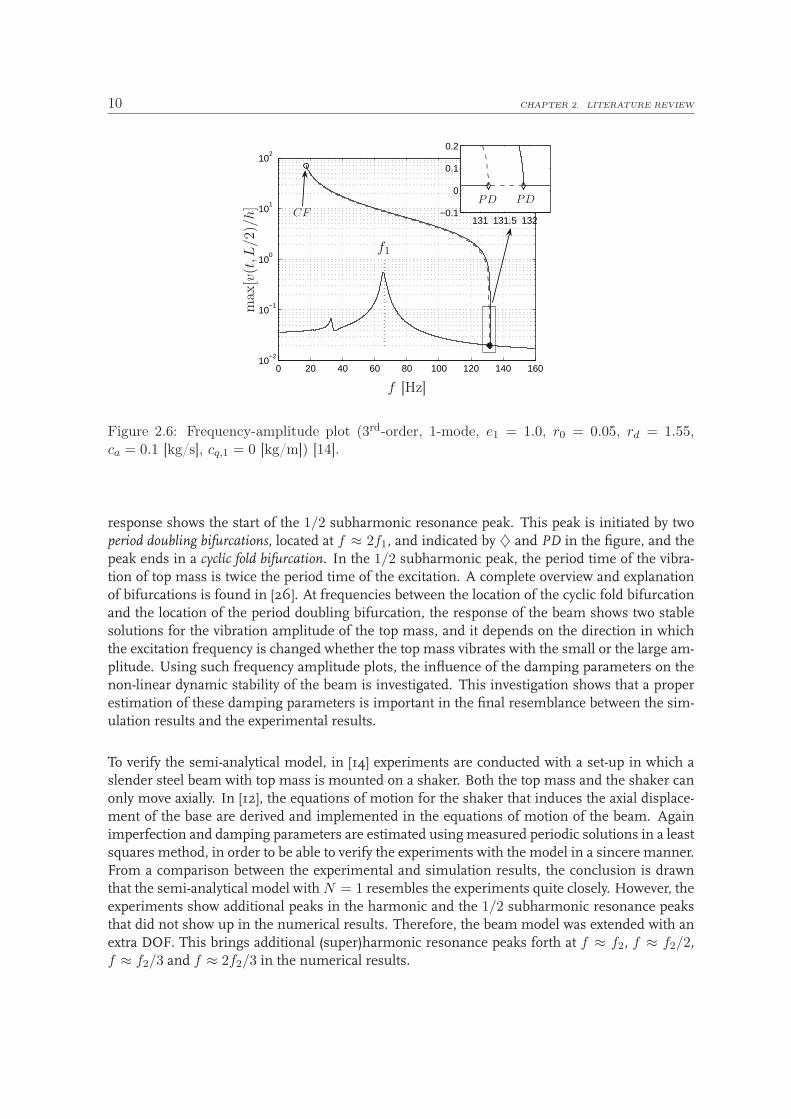
10 CHAPTER 2. LITERATURE REVIEW
0 20 40 60 80 100 120 140 16010
−2
10−1
100
101
102
131 131.5 132−0.1
0
0.1
0.2
f [Hz]
f1m
ax[v
(t,L
/2)/
h]
PD PDCF
Figure 2.6: Frequency-amplitude plot (3rd-order, 1-mode, e1 = 1.0, r0 = 0.05, rd = 1.55,ca = 0.1 [kg/s], cq,1 = 0 [kg/m]) [14].
response shows the start of the 1/2 subharmonic resonance peak. This peak is initiated by twoperiod doubling bifurcations, located at f ≈ 2f1, and indicated by ♦ and PD in the figure, and thepeak ends in a cyclic fold bifurcation. In the 1/2 subharmonic peak, the period time of the vibra-tion of top mass is twice the period time of the excitation. A complete overview and explanationof bifurcations is found in [26]. At frequencies between the location of the cyclic fold bifurcationand the location of the period doubling bifurcation, the response of the beam shows two stablesolutions for the vibration amplitude of the top mass, and it depends on the direction in whichthe excitation frequency is changed whether the top mass vibrates with the small or the large am-plitude. Using such frequency amplitude plots, the influence of the damping parameters on thenon-linear dynamic stability of the beam is investigated. This investigation shows that a properestimation of these damping parameters is important in the final resemblance between the sim-ulation results and the experimental results.
To verify the semi-analytical model, in [14] experiments are conducted with a set-up in which aslender steel beam with top mass is mounted on a shaker. Both the top mass and the shaker canonly move axially. In [12], the equations of motion for the shaker that induces the axial displace-ment of the base are derived and implemented in the equations of motion of the beam. Againimperfection and damping parameters are estimated using measured periodic solutions in a leastsquares method, in order to be able to verify the experiments with the model in a sincere manner.From a comparison between the experimental and simulation results, the conclusion is drawnthat the semi-analytical model with N = 1 resembles the experiments quite closely. However, theexperiments show additional peaks in the harmonic and the 1/2 subharmonic resonance peaksthat did not show up in the numerical results. Therefore, the beam model was extended with anextra DOF. This brings additional (super)harmonic resonance peaks forth at f ≈ f2, f ≈ f2/2,f ≈ f2/3 and f ≈ 2f2/3 in the numerical results.

2.4. OVERVIEW OF DYNAMIC BUCKLING ANALYSIS 11
The previously mentioned investigations focus on the non-linear dynamic stability of the slenderbeam with small relative top mass. The isolation property of the beam is not investigated becausethe beam can only act as a vibration isolator if it is in post-buckling state, i.e. when heavier topmasses are applied. As the isolating functioning of a buckled beam is the topic of the presentresearch, the next section discusses the isolating capability of the buckled beam.
2.4.2 Vibration isolation using buckled beams
Buckled beams subjected to an axial harmonic excitation are theoretically investigated in [22]. Inthis paper, the clamped-clamped beam is assumed to have a sinusoidal shaped geometrical im-perfection, and the beam is subjected to a static top load and a harmonic axial excitation. Afterdefining the free-body diagram of an element of the column, the equations that describe the staticand inertia forces on the element are derived. The static equilibrium configuration is analyzedusing these equations and a shooting method, and the linear dynamics of the beam with smallsteady-state vibrations around the equilibrium is investigated. The transmissibility of the buckledbeam is defined as the ratio of the amplitude of the axial motion of the top load to the amplitudeof the axial motion applied at the base of the beam. This ratio should be much smaller thanone for a large range of excitation frequencies, in order for the beam to be useful as vibrationisolator. First, the transmissibility is investigated by varying the so-called stiffness parameter, de-fined as EI/(mbeamgL2), the imperfection, and the internal damping parameter. It follows thatthe frequency range in which the transmissibility is smaller than one increases with decreasingstiffness, and that the transmissibility for f > f1 decreases for decreasing internal damping.Furthermore, analyses show that, when the top load is smaller than the Euler buckling load, anincrease in imperfection of the beam results in a higher frequency range in which the beam actsas a vibration isolator. However, when this top load reaches or exceeds the critical top load, thebeam should be as perfect as possible in order to get a very low transmissibility and large utilityrange.
In [28], the theoretical steady-state displacement transmissibility of a pinned-pinned buckledbeam is compared to experiments. The transmissibility as used in [28] is given as:
X
Y=
[
1 + (2ζΩ)2
(1− Ω2)2 + (2ζΩ)2
]1/2
, (2.1)
with X the amplitude of the top mass, Y the excitation amplitude, ζ the damping ratio and Ωis the ratio between the excitation frequency and the eigen frequency, Ω = ω/ωn. From thisequation, it follows that the transmissibility is smaller than 1 if Ω >
√2. To validate whether this
also holds for buckled beams, a set-up is constructed, consisting of two parallel pinned-pinnedbuckled beams mounted between a vertical shaker and fixed top mass of 2.4 [kg]. This top loadis close to the Euler buckling load for the beams used, which is 2.55 [kg]. Furthermore, theexcitation amplitude is set to 3 [mm] and the frequency range is between approximately 1.3Ωand 7.8Ω. From the experiments, it follows that indeed the transmissibility is smaller than 1 forfrequencies higher than
√2Ω, although isolation also occurs at frequencies slightly smaller than√
2Ω. At f ≈ 7.8Ω a transmissibility of ≈ 0.02 is accomplished. It is stressed that, as in [22], onlythe linear dynamics of this beam are investigated.

12 CHAPTER 2. LITERATURE REVIEW
2.5 Conclusions
References [12, 14] discussed in Sections 2.3 provide the foundation of the research presented inthis thesis. Theory described in these theses forms the basis of Chapters 3 and 4. The literaturediscussed in Section 2.4.2 mainly focus on the linear dynamics of the buckled beam. In this the-sis, the non-linear dynamics of the buckled beam with large relative top mass is investigated, andforms this way a supplement to the current investigations on using buckled beams as vibrationisolators.

Chapter 3
A semi-analytical model for buckling
of beams
As discussed in the previous chapter, buckling beams can be used as vibration isolators by po-sitioning them between a vibrating support and a structure, in this case a mass, that has to beisolated from the support. Figure 3.1 shows an example of a slender beam with a vibrating baseand a top mass. In this figure, the beam with width b, length L and thickness h≪ L is clampedon one end to the shaker, and on the other end to a top mass mt. Both ends are thus restrainedin all rotational directions, and in the x and z direction; the clamps of the beam can only movein y-direction. The beam exhibits an initial geometrical imperfection v0(y), and the transversaldisplacement v(t, y) of a point along the beam at position y and time t is relative to this initial im-perfection. Furthermore, the axial displacement of the shaker is indicated by us(t) and the axialdisplacement of the top mass is defined as ut(t) = us(t) + u(t, L); u(t, y) is the axial displace-ment at position y relative to the shaker displacement us(t). This beam and the aforementionednotations are used throughout this thesis.
u(t, y)
mtut(t)
v0(y) v(t, y)
x
y
g
h
us(t)
z
Figure 3.1: Base-excited thin beam with top mass.
13

14 CHAPTER 3. A SEMI-ANALYTICAL MODEL FOR BUCKLING OF BEAMS
This chapter is organized as follows: In Section 3.1, the static buckling phenomenon is intro-duced. Section 3.2 discusses themodeling of a buckled beam and derives the equations of motion.In Section 3.3, the static response of the buckled beam is analyzed using the model presented inSection 3.2 by varying the weight of the top mass. The results are compared to Finite ElementAnalysis (FEA) results to verify the model. The FE package MSC.Marc [19] is used in this. Sec-tion 3.4 sets the boundaries for the axial and transversal displacement of a beam in order to avoidplastic deformation. A comparison between the modal analysis of the semi-analytical model andresults of the FEA is made in Section 3.5. Finally, Section 3.6 gives a brief summary of thischapter.
3.1 Critical static buckling load
Theoretically, a beam buckles if the axial load on the beam is larger than the first static bucklingload of the beam. The first static buckling load for a clamped-clamped column is derived in [16]and is
Pc,inext =4π2EIx
L2, (3.1)
for inextensible columns and
Pc,ext = EA1−
√
1− 16π2Ix
AL2
2, (3.2)
for extensible columns. Pc,inext is also called the Euler buckling load. In these equations, E repre-sents the Young’s modulus and Ix the second moment of area around the x-axis. For very slender
beams, such as the beam considered in this thesis,1−
√
1− 16π2IxAL2
2 ≈ 4π2Ix
AL2 and Pc,inext ≈ Pc,ext.In this thesis, the beam is considered to be inextensible: as a result of its slenderness, displace-ments are dominated by changes in the beam’s curvature, rather than changes in the geometry.Throughout this thesis, the addition ,inext is omitted and the critical buckling load is indicated byPc.
The first static buckling loads in (3.1) and (3.2) apply only to geometrically perfect columns. Inreality, however, a beam will always exhibit an initial geometrical imperfection. This geometri-cal imperfection results in buckling far before the critical top load according to (3.1) or (3.2) isapplied, which is discussed more elaborately in Section 3.3.
3.2 Equations of motion
This section discusses the dynamic modeling of the buckled beam of Figure 3.1 and is basedon [12, 14] to a large extent. First, the kinetic and potential energy are derived. Subsequently, thediscretization of the transversal displacement field of the beam is formulated, resulting in a setof equations of motion.

3.2. EQUATIONS OF MOTION 15
The equations of motion for the clamped-clamped beam with top mass are derived using La-grange’s equations of motion [12]:
d
dt
(
T,Q
)
− T,Q + V,Q = (Qnc) , (3.3)
with T the kinetic energy, V the potential energy, Q = [Q1, .., QN ]T the column with N general-ized coordinates (also referred to as degrees of freedom or DOFs) and Qnc the non-conservativegeneralized external forces due to a Raleigh dissipation function Db, Q
nc = −Db,Q. The kineticenergy T of the beam with top mass consists of two parts: one part results from bending of thebeam and the other part contains the contribution of the vibrating top mass. The axial inertia ofthe beam is neglected in this equation as mt ≫ mbeam, the mass of the beam. The kinetic energyis therefore:
Tb(Q, Q) =1
2ρA
∫ L
0v2dy +
1
2mt (us + u(t, L))2 , (3.4)
with ρ the mass density of the material of the steel beam and A = bh the cross section of thebeam.The potential energy V consists of a term that describes the strain energy due to bendingof the beam and a term representing the potential energy of the top mass due to the gravityacceleration g = 9.81 [m/s2]. Due to the slenderness of the beam (h ≪ L), the transversal shearof the beam is negligible in the potential energy:
Vb(Q) =1
2EIx
∫ L
0(κ− κ0)
2dy + mtg (us + u(t, L)) , (3.5)
with E the Young’s modulus of steel, Ix = bh3/12, κ the curvature of the beam, and κ0 the initialcurvature of the beam due to the initial imperfection v0(y). κ and κ0 are derived later on. TheRaleigh energy dissipation function is assumed to be:
Db(Q) =N
∑
i=1
(
1
2ciQ
2i +
1
3cq,isign(Qi)Q
3i
)
. (3.6)
In this equation, ci is the linear viscous damping constant of mode i and cq,i is the quadraticviscous damping constant of mode i. It should be noted that Tb, Vb, and Db depend on Q and/orQ because u(t, y) and v(t, y) depend on Q and/or Q as is shown next.
The transversal displacement field v(t, y) of the beam is approximated using the assumed modesmethod. This method assumes that the displacement field can be discretized using a linearcombination of N modes vi(y) (i = 1, 2, ..., N ) and corresponding generalized coordinates Qi(t):
v(t, y) =N
∑
i=1
Qi(t)vi(y). (3.7)
Each mode vi(y) should obey the following boundary conditions a priori:
v(0) = v(L) = 0, (3.8)
v,y(0) = v,y(L) = 0. (3.9)

16 CHAPTER 3. A SEMI-ANALYTICAL MODEL FOR BUCKLING OF BEAMS
mode 1 mode 2 mode 3
Figure 3.2: The first three mode shapes.
The following shapes for vi(y) are proposed, which fulfil the boundary conditions (3.8) and (3.9):
vi(y) = cos
(
(i− 1)πy
L
)
− cos
(
(i + 1)πy
L
)
. (3.10)
The first three mode shapes are depicted in Figure 3.2. The geometrical imperfection is dis-cretized similarly by:
v0(y) =
Ne∑
i=1
1
2heivi(y), (3.11)
with ei the dimensionless imperfection parameter for shape vi and Ne ≤ N .
The relative axial displacement u(t, y) is fully determined by v(t, y) and v0(y) when using theassumption that the beam is inextensible. The deformed length ds of an infinitesimally smallpiece of the beam thus equals the initial length ds0 of this infinitesimally small piece. By using
Figure 3.3, it can be shown that ds0 =√
1 + v20,y
dy and ds =√
(1 + u,y)2 + (v0,y + v,y)2dy, and
the following inextensibility constraint is derived:
u,y =√
1− 2v0,yv,y − v2,y − 1. (3.12)
This non-linear expression can in principle be integrated over y to obtain u(t, y).
ds0 dy
v0,ydy
dsdy + u,ydy
(v0,y + v,y)dy
(a) (b)
Figure 3.3: The initial length (a) and deformed length (b) of an infinitesimally small piece ofthe beam.

3.3. STATIC RESPONSE 17
The non-linear inextensibility constraint (3.12) is not the only reason why the equations of motionbecome non-linear. The curvature of the centerline of the deformed beam can be formulatedusing the expression for the curvature of a general curve as defined in [10]:
κ(t, y) =X(t, y),yY (t, y),yy −X(t, y),yyY (t, y),y
(
X(t, y)2,y + Y (t, y)2,y)
3
2
, (3.13)
with X(t, y) = v0(y) + v(t, y) and Y (t, y) = y + us(t) + u(t, y) following from Figure 3.1.Substitution of X(t, y) and Y (t, y) in (3.13) results in the following non-linear expression for thecurvature of the beam:
κ(t, y) =−v0,yy − v,yy + v0,yv0,yyv,y − v2
0,yv,yy√
1− 2v0,yv,y − v2,y(1 + v2
0,y)3
2
. (3.14)
The initial curvature of the beam is
κ0(y) =−v0,yy
(1 + v20,y)
3
2
. (3.15)
From (3.4) and (3.5), it follows that in order to compute Lagrange’s equations, both the inex-tensibility constraint from (3.12) and the curvature in (3.14) need to be integrated. However,for both expressions it is not possible to analytically compute the exact integral because of thechoices (3.10) and (3.11). Therefore, Taylor series approximations are used to approximate u,y
and κ(t, y). It is chosen to develop the approximation around the unloaded configuration, insteadof around the buckled situation. Appendix A explains this at first glance maybe unusual choice,and other consequences of the choice to use Taylor series approximation.
The equations ofmotion in (3.3) are now symbolically derived using the software packageMAPLE[15], and they are used in the next section in the analysis of the static response.
3.3 Static response
The static response of the buckled beam is analyzed by varying the weight of the top mass. In theequations of motion, derived in Section 3.2, all time dependent terms are omitted. First, the axialand transversal displacement are evaluated as function of the top load, after which the resultsare compared to Finite Element Analysis (FEA) results to verify the model. The FE packageMSC.Marc [19] is used in this.
3.3.1 Load path
To analyze the static response, us(t) = 0 [m/s2] and all time-dependent terms are set to zero.The parameters used in this analysis are shown in Table 3.1. The values for E and ρ are for steel.The beam’s dimensions are chosen identical to the beam in [12], as this beam is used to carry outexperiments in Chapter 5. The relative, normalized transversal displacement v(L/2)/L and therelative, normalized axial displacement u(L)/L, both derived in Section 3.2, are plotted againstthe relative top load r0 in Figures 3.4a and 3.4b respectively, with
r0 =mtg
Pc. (3.16)

18 CHAPTER 3. A SEMI-ANALYTICAL MODEL FOR BUCKLING OF BEAMS
Table 3.1: The parameters used in the static response analyses.
L 0.18 [m]h 5 · 10−4 [m]b 1.5 · 10−3 [m]E 2.1 · 1011 [N/m2]ρ 7850 [kg/m3]e1 1 [-]
The semi-analytical model with N = 1 is used in these figures. The results are compared toFEA results. The FEM-model is built using 50 3-node Timoshenko beam elements, i.e. elementtype 45 [18] in MSC.Marc. The FEA is carried out using kinematic relations for large displace-ments and large rotations, and using the upgraded Lagrange formulation. The thin solid blackline in Figures 3.4a and 3.4b shows the relative transversal and axial displacement respectivelyif the beam is assumed to be perfectly straight, ie e1 = 0 [-], using a third order Taylor seriesapproximation. Clearly, the beam buckles at r0 = 1 [-] as expected and tends to approach theblack dashed curve, representing a third order Taylor series approximation with an imperfectionof e1 = 1 [-]. The other three thick non-solid lines represent the load-path for an imperfect beamwith e1 = 1 [-] and using different orders in Taylor series approximation, namely a fifth, a ninthand a thirteenth order approximation, respectively. The closest resemblance to the FEM-model,shown in the thick solid curve, is achieved by the highest Taylor series approximation.
0 0.2 0.4 0.60
0.5
1
1.5
2
v(L/2)/L [-]
r 0[-]
3rd order, e1=0 [-]3rd order, e1 = 1 [-]5th order, e1 = 1 [-]9th order, e1 = 1 [-]13th order, e1 = 1 [-]FEM-model, e1 = 1 [-]
0 0.050.7
0.8
0.9
1
v(L/2)/L [-]
r 0
(a) Relative transversal displacement at y = L/2 [-] with close-up
−1 −0.8 −0.6 −0.4 −0.2 00
0.5
1
1.5
2
u(L)/L [-]
r 0[-]
3rd order, e1 = 0 [-]3rd order, e1 = 1 [-]5th order, e1 = 1 [-]9th order, e1 = 1 [-]13th order, e1 = 1 [-]FEM-model, e1 = 1 [-]
−2 −1 0x 10
−3
0.7
0.8
0.9
1
r 0
(b) Relative axial displacement at y = L [-] with close-up
0 0.02 0.04 0.06 0.080
0.02
0.04
0.06
0.08
0.1
0.12
0.14
0.16
0.18
← r0 = 0
X [m]
Y[m
]
← r0 = 0.98
↓ r0 = 1.82
(c) Beam shapes, FEA
Figure 3.4: The static load path, and corresponding beam shapes with e1 = 1 [-].

3.3. STATIC RESPONSE 19
Furthermore, two other conclusions are drawn from Figures 3.4a and 3.4b. First, in the FE anal-ysis v(L/2)/L tends to decrease for a relative top mass of r0 > 1.8 [-]. At this point, a physicallyimpossible situation occurs. The upper clamp of the beam approaches its lower clamp so muchthat the beam adopts a loop shape, in which it touches itself. This is shown by the light grayline in Figure 3.4c (r0 = 1.82 [-]). As contact is not taken into account in the FEA, the upperclamp keeps moving downwards with increasing top mass, and the beam moves ‘through itself’.This is physically impossible, and the results for top loads higher than r0 = 1.82 [-] should beneglected. In Figure 3.4c, the beam shape shown in black near the y-axis reflects the initial geo-metrical imperfection (e1 = 1 [-]), and the dark gray line shows the beam shape when the criticalbuckling load is almost reached (r0 = 0.98 [-]). An obvious thought rising from the most extremebeam shape is whether the material is plastically deformed, and if so, what maximum weight,and corresponding transversal and axial displacements, the beam can handle prior to plastic de-formation. This is discussed later on in Section 3.4.
Second, for r0 > 1.02 [-], the load paths obtained by the semi-analytical models using an initialimperfection of e1 = 1 [-] deviate from the FEA curve, which is for the largest part a resultof the Taylor series approximations of (3.12) and (3.14), as mentioned before and explained inAppendix A, and also due to the axial strain and transversal shear that are taken into account onlyin the FE analysis. Moreover, the choice of the mode shape presented in (3.10) can also lead toerrors when this representation shows poor coherence to the exact static transversal displacementfield. This indicates that results from the semi-analytical model should be handled with care, if atop load larger than r0 ≈ 1 is used. The relative error between the load paths computed by FEAand the semi-analytical model, using the beam parameters as defined in table 3.1, is defined as
ε% =vanalytic − vFEA
vFEA100%. (3.17)
The relative error is plotted in Figure 3.5a for the transversal displacement v(L/2) and in Fig-ure 3.5b for the axial displacement u(L). The relative error ε% in axial displacement is very largefor r0 < 0.8 [-]. Figure 3.5c, however, shows that the absolute error is very small here, namelyεO10−6 [m]. The relative error in axial displacement is larger than the relative error in transver-sal displacement. This is due to the choice of the mode shapes as defined in (3.10), which hasa larger influence on the axial displacement u(L) than on the transversal displacement v(L) itself.
0 10 20 30 40 500
0.5
1
ε%
r 0[−
]
3rd order5th order9th order13th order
(a) Error [%] in transversal displacement
0 20 40 60 800
0.5
1
ε%
r 0[−
]
3rd order5th order9th order13th order
(b) Error [%] in axial displacement
−5 0x 10
−6
0
0.2
0.4
0.6
0.8
ε [m]
(c) Absolute error
Figure 3.5: Error between the model with N = 1 and the FEM-model, e1 = 1 [-].

20 CHAPTER 3. A SEMI-ANALYTICAL MODEL FOR BUCKLING OF BEAMS
As a last remark, it should be noted that, obviously, the ratio v(L/2)/L cannot reach 0.5, sincethis would imply that the beam is folded in two parallel parts with a plastic hinge. Although itfollows from Figure 3.4a that v(L/2)/L does not approach 0.5, it should be investigated at whatmaximum transversal deflection the beam will deform plastically, also considering the extremebeam shape in Figure 3.4c. This is discussed in Section 3.4.
3.4 Plastic deformation
In [12, 14], small relative top masses are applied to the beam (r0 < 0.25 [-]), and consequentlythe beam only bends slightly. Therefore, plastic deformation was not a topic of discussion. How-ever, in this research large relative top masses are applied resulting in increased bending of thebeam. In Section 3.3, static force-displacement curves have been discussed. At some point in theforce-displacement curve, plastic deformation will occur. In this project, it has been decided toinvestigate vibration isolation capabilities of a buckled beam without plastic deformation. There-fore, the occurrence of plastic deformation should be avoided. In this section, it is examinedat which deflections plastic deformation will occur, so that it becomes clear what the maximumallowed deflections are.
3.4.1 Maximum beam deflection
When a load is applied to a structure, it deforms. The deformation remains purely elastic, whenthe stress remains smaller than the yield stress of the material. If the stress applied exceedsthis yield stress, the material will deform plastically. In Figure 3.6, a typical relation betweenengineering stress and strain of steel is shown, [2]. In a uni-axial situation, the elastic stress σe
and elastic strain ǫe in a material are linearly related to each other according to Hooke’s law:
σe = ǫeE. (3.18)
This is the curve between points 1 and 2 in Figure 3.6. When the yield stress is exceeded, thematerial starts to deform plastically in a non-linear fashion at point 3. If subsequently the loadis removed, the material remains deformed. The stress at this point is called the yield stress σy,
σyσbσn
ǫy ǫbǫnǫp = 0.002
σ
ǫ
EE
1
2
3
4
5
Figure 3.6: Stress-strain curve for steel.

3.4. PLASTIC DEFORMATION 21
which is determined using the 0.002 strain offset method, [2]: the stress at 0.2% plastic strainis the yield stress. At this point, plastic deformation has thus already occurred, but as it is diffi-cult to determine smaller strains, this is the general accepted method. When the stress is keptincreasing, at some point necking occurs, indicated by 4 in the figure. The corresponding stressσn is called the tensile strength. Eventually, the material will fail completely and it breaks at point5. The final strain of the material at this point is indicated by ǫb, and the stress applied is indi-cated by σb. In order to remain in the elastic region of the stress-strain curve, the stress in thebeam should be smaller than the yield stress σy, and ǫe <
σy
E . The Young’s modulus E of steelis 2.1 · 1011 [N/m2] and the yield stress σy is in the range 250 − 500 · 106 [N/m2], depending onthe type of steel. In Figure 3.7a, a part of a buckled beam is shown. In this figure, the dashedline represents the neutral axis of the beam. It is assumed that this axis does not experience anystrain. The radius of the curvature of the beam at position y is indicated by ρ(y). The strain dueto bending of the beam is:
ǫ =L− L0
L0, (3.19)
with L0 the initial length, which is considered to be 2πρ(y), and L the deformed length, whichequals 2π(ρ(y)± h/2). The strain due to bending is thus:
ǫ = ± h
2ρ(y). (3.20)
The relation between the curvature κ(y) of the centerline of the buckled beam and its radius isgiven in [10]:
ρ(y) =1
|κ(y)| , (3.21)
with κ(y) as defined in (3.14). Consequently, the strain in the beam reaches maximum at max|κ|,which occurs for the case N = 1 at y = 0, y = L/2 and y = L, as follows from Figure 3.7b. Inthis figure, the curvature along the y-axis of a beam with length L = 0.18 [m], initial imperfection
ρ(y)
hy
x(a) Part of a bent beam
−40 −20 0 20 400
0.06
0.12
0.18
κ [1/m]
Pos
itio
ny
[m]
(b) The curvature of a bent beam along they-axis
Figure 3.7: Shape and curvature of a bent beam.

22 CHAPTER 3. A SEMI-ANALYTICAL MODEL FOR BUCKLING OF BEAMS
of e1 = 1 [-] and generalized coordinate Q1 = 0.025 [m] is shown. Substitution of y = L/2 andQ1 = v(L/2)/2 (following from (3.10)) in (3.14) gives:
κ(y = L/2) =(
v(L/2) + e1h)2π2
L2. (3.22)
Using (3.18), (3.20),(3.21), and (3.22), the maximum transversal deflection at y = L/2 for whichthe strain is purely elastic is obtained:
vmax =σyL
2
Ehπ2− e1h. (3.23)
Furthermore, a third order Taylor series approximation of the maximum axial displacement of thetop load relative to the base is obtained by integration of (the 3rd order Taylor series approximationof) (3.12):
u(L) = −π2Q1(e1h + Q1)
L. (3.24)
Substitution of Q1 = vmax/2 in (3.24) gives:
umax = −π2vmax(2e1h + vmax)
4L. (3.25)
The theoretical maximum transversal and axial deflections are compared to FEA results to verifytheir accuracies. In the FEM-model, elasto-plastic material behavior is taken into account and itis assumed that when the yield stress is exceeded, the beam exhibits linear hardening accordingto the following model [9]:
σv = σv0 + Hǫp, (3.26)
with σv0 the elastic stress, ǫp the effective plastic strain and H the hardening constant. The curve
in the plastic region of the stress strain curve in Figure 3.6 (i.e. the curve between points 2 and4) is thus assumed to be linear. It is assumed that the following relation between the hardeningconstant and the Young’s modulus holds: H = E/20 [24]. The value of the transversal deflectionof the beam (at y = L/2), calculated by FE analysis, at which the strain in the beam equals theyield strain ǫy = σy/E, is compared to results from (3.23) and (3.25) in Table 3.2 for variousvalues for the length and thickness of the buckled beam. In this analysis, an initial imperfectionof e1 = 1 [-] is assumed and the yield stress σy is chosen to be 500·106 [N/m2]. Table 3.3a shows therelative error ε% in terms of percentage between themaximum transversal displacement obtainedfrom the FEA results and (3.23). Table 3.3b shows this error for umax. From these tables, it followsthat (3.23) and (3.25) are not accurate for very slender beams (L > 2000h) because then the massof the beam has a significant influence on the point of buckling, and this mass is neglected in thesemi-analytical model for the axial direction. Very slender beams even suffer from self-buckling:they are not able to hold their own weight. More information on the influence of the beam’sself-weight on buckling is found in [27]. Furthermore, in beams with L < 200h stresses due totransversal shear may start to play a role; an effect that is also not taken into account in (3.4) and(3.5). The most important explanation for the error between the results from the semi-analyticalmodel and the FEA is the fact that the shape function as assumed in (3.10) does not represent theexact static transversal displacement field. Moreover, in the computation of umax, only a 3rd order

3.4. PLASTIC DEFORMATION 23
Table 3.2: The error ε% in terms of percentage between vmax and umax obtained from (3.23)and (3.25) respectively and the results from the FEA, e1 = 1 [-] and σy = 500 · 106 [N/m2].
L [m] h [m] 0.0001 0.0003 0.0005 0.001
0.13 12.65 1.13 -2.45 -17.500.18 25.32 2.16 0.47 -1.010.23 N/A 4.17 1.08 -1.410.28 N/A 6.33 1.91 -1.730.50 N/A 21.44 7.37 0.981.00 N/A N/A N/A 7.41
(a) Error ε% in vmax
L [m] h [m] 0.0001 0.0003 0.0005 0.001
0.13 9.02 0.43 -5.62 -30.460.18 17.79 0.91 -0.41 -3.910.23 N/A 2.79 0.12 -3.790.28 N/A 4.38 0.83 -4.310.50 N/A 14.23 5.03 -0.471.00 N/A N/A N/A 4.78
(b) Error ε% in umax
Taylor series approximation is used. From Table 3.2, it follows that the maximum transversal andaxial deflection predicting the onset of plastic deformation can be roughly estimated using (3.23)and (3.25) for 200h < L < 2000h.
In Figure 3.8a, the static response of the FEM-model with inclusion of elasto-plastic materialbehavior is shown for a beam length of L = 0.18 [m], σy = 500 · 106 [N/m2] and e1 = 1 [-].For each beam three different values for the beam thickness are used, namely h = 0.0003 [m],h = 0.0005 [m] and h = 0.001 [m], represented by the solid line, the dashed line and the dottedline respectively. For all curves holds that plastic deformation starts at points where the maxi-mum r0 values are found. From the dashed line in Figure 3.8a (h = 0.0005 [m]), it follows thatthe beam starts to deform plastically slightly before the critical top load (r0 = 1 [-]) for the perfectbeam (e1 = 0 [-]) is reached; this is the beam used in the investigations of [12, 14] and which isalso used in this report. Decreasing the thickness of the beam to h = 0.0003 [m], indicates someimprovement as plastic deformation occurs at a top load larger than the critical load. Increasingthe thickness of the beam to h = 0.001 [m], results in plastic deformation at a top load of only90% of the relative top mass. In Figure 3.8b the length of the beam is increased to L = 0.50 [m].For h = 0.0005 [m] this enables the use of a top load that exceeds the critical load (for the perfect
0 0.5 1 1.5 2 2.5x 10
−3
0
0.25
0.5
0.75
1
1.25
r 0[-]
v(L/2)/L [-]
h=0.0003 [m]h=0.0005 [m]h=0.001 [m]
(a) L = 0.18 [m]
0 0.5 1 1.5 2 2.5x 10
−3
0
0.25
0.5
0.75
1
1.25
r 0[-]
v(L/2)/L [-]
h=0.0003 [m]h=0.0005 [m]h=0.001 [m]
(b) L = 0.50 [m]
Figure 3.8: Load path taking elasto-plastic material behavior into account.

24 CHAPTER 3. A SEMI-ANALYTICAL MODEL FOR BUCKLING OF BEAMS
structure) before plastic deformation occurs. Again variations in the thickness of the beam areapplied and again it appears that the top load at which the beam deforms plastically increaseswith decreasing thickness. In all curves, two sharp bends show up in the load path: the first bendoccurs at the point of plastic deformation, the second bend cannot be explained at this moment.However, this is not of importance in this research.
The maximum axial and transversal displacement of a buckled beam prior to plastic deformationhave been derived in this section. The yield stress σy is estimated in this analysis. Therefore, thenext section determines the yield stress σy for the beam used in the experiments in Chapter 5.
3.4.2 Static experimental results
To experimentally validate the yield stress σy of the beam, a beam with thickness h = 0.0005 [m]and length L = 0.183 [m] is axially loaded with a gradually increasing top mass. After each step,the axial displacement is measured, see Figure 3.9. In this figure, the measurement points areindicated by the black x-marks and the load path computed by the 1-DOF semi-analytical modelis indicated by the solid black line. A 13th order Taylor series approximation is used to obtainthe axial displacement. The left y-axis indicates the top mass [kg] applied and on the right y-axisthe corresponding relative top mass r0 [-] is indicated. In the experiment, the axial displacementincreases rapidly between an applied top mass of 3.269 [kg] and a top mass of 3.308 [kg]; appli-cation of an even heavier top mass leads to complete failure of the beam. Therefore, it is verylikely that plastic deformation of the beam occurs around mt ≈ 3.28 [kg]. The beam parame-ters used in the model are found in Table 3.3. In [12], a least squares method is used to estimate
−0.018 −0.015 −0.012 −0.009 −0.006 −0.003 00
0.1
0.2
0.3
0.4
0.5
0.6
0.7
0.8
0.9
r 0[-]
−0.018 −0.015 −0.012 −0.009 −0.006 −0.003 00
0.5
1
1.5
2
2.5
3
3.5
4
mt
[kg]
u(L) [m]
measurementmodel N = 1
Figure 3.9: Experimental determination of σy.

3.5. MODAL ANALYSIS 25
Table 3.3: The parameters used to fit the model to the static experimental results.
L 0.183 [m]h 4.95 · 10−4 [m]b 1.5 · 10−3 [m]E 1.9 · 1011 [N/m2]ρ 7850 [kg/m3]e1 1.4 [-]
the Young’s modulus E and the initial imperfection parameter e1 from the experiments. In thisidentification process, a Young’s modulus of E = 1.9 · 1011 [N/m2] is found, which is explainedby the non-ideal clamping of the beam. As the set-up is identical to the one in [12], and the beamused in the experiment of Figure 3.9 is produced from the same material as used in [12], andvery likely even from the same batch of material, it is assumed that the parameter value for theYoung’s modulus can also be used for this beam. The measured length of the clamped-clampedbeam is L = 0.183 [m]. The initial imperfection is measured before the beam was mounted intothe set-up and is e1 = 1.4 [-]. Observations show that the beam has an initial geometrical imper-fection according to the first mode shape as defined in (3.10). It follows that the beam propertiesfrom Table 3.3 result in a proper fit between the semi-analytical model with N = 1 and a 13th
order Taylor series approximation to the experimental results for top masses smaller than the topmass at which the beam starts to deform plastically. Assuming that plastic deformation starts atmt = 3.28 [kg] and using (3.25), σy ≈ 4.6·108 [N/m2], so the initial guess of σy = 5·108 [N/m2] asused in Figure 3.8 is slightly overrated. However, it should be noted that changes in estimationsof e1 and the Young’s modulus lead to a somewhat different estimation of σy. Furthermore, theaccuracy of (3.25) may be moderate due to the 3rd order Taylor series approximation used.
3.5 Modal analysis
The eigenfrequencies of the beamwith topmass are calculated by linearizing the equations ofmo-tion in the semi-analytical model of the beam around several equilibrium states, i.e. for variousloads r0, and by solving the corresponding eigenvalue problems for the undamped system. Theseeigenfrequencies are compared to the eigenfrequencies obtained using finite element analysis(FEA), see Figure 3.10a. In Figure 3.10b, a close-up of the first eigenfrequency is provided. In thiscomparison, two different semi-analytical models are used, namely a using N = 1 and N = 3,and a range of top loads between r0 = 0.05 and r0 = 1.6 [-]. In these calculations, a geometricalimperfection is taken into account only in the first DOF, i.e. e1 = 1 [-]; for higher modes in theshape function the corresponding imperfection parameters are set to zero, i.e. e2 = e3 = 0 [-]. InFigure 3.10a, the results for model with N = 1 are shown in black triangles. The results of themodel with N = 3 are shown in black circles for the first eigenfrequency, in black x-marks forthe second eigenfrequency, and in black squares for the third eigenfrequency. For the first threeeigenfrequencies of the FEA, the same markers are used but now in gray. From Figure 3.10b itfollows that the first eigenfrequency f1 of both the model with N = 1 and the model with N = 3,and the FEA lie very close to each other for relative top masses r0 < 0.9 [-]. This observationwas also made in [14] in the modal analysis. However, in [14], as only beams with small relative

26 CHAPTER 3. A SEMI-ANALYTICAL MODEL FOR BUCKLING OF BEAMS
0 100 200 300 400 5000
0.2
0.4
0.6
0.8
1
1.2
1.4
1.6
f [Hz]
r 0[-]
1 DOF, f1
3 DOF, f1
3 DOF, f2
3 DOF, f3
FEM, f1
FEM, f2
FEM, f3
(a)
0 10 20 30 40 500
0.2
0.4
0.6
0.8
1
1.2
1.4
1.6
f [Hz]
r 0[-]
1 DOF, f1
3 DOF, f1
3 DOF, f2
3 DOF, f3
FEM, f1
FEM, f2
FEM, f3
(b)
Figure 3.10: The first three eigenfrequencies based on the SA-model with N = 1, the SA-model with N = 3, and the FEM-model, with a close-up for the first eigenfrequencies on theright hand side.
top masses were considered, the analysis was done for r0 = 0.05 and r0 = 0.5, instead of thecomplete range presented here. For higher relative top masses, however, the relative differencebetween the results of the FEA and the semi-analytical models increases. Furthermore, the sec-ond eigenfrequencies computed by the FEA deviate from the 3-DOFmodel, for r0 > 0.95 [-]. Thisis due to the fact that the FEA does not determine whether the static solution is stable or not. Inthis case, for r0 > 0.95, the eigenfrequencies of the unstable static solution are found by the FEA,while the model with N = 3 computes the eigenfrequencies of the stable static solution. Moreinformation on this is found in Appendix B. In the comparison of the third eigenfrequencies forrelative top masses smaller than the critical buckling load, poor correspondence is found betweenthe model with N = 3 and the FEA. From this figure, the conclusion is drawn that especially theresults for the third eigenfrequencies should be handled with care.
(a) Mode shapes for r0 = 0.5 [-] (b) Mode shapes for r0 = 1.2 [-]
Figure 3.11: The first three mode shapes from the model with N = 3 (black lines) and theFEA (gray dashed lines) for two different values for r0, with e1 = 1 [-].

3.6. SUMMARY 27
The three mode shapes of the beam with top mass computed by the semi-analytical model withN = 3 are compared to the first three mode shapes obtained from the FEA in Figure 3.11. In Fig-ure 3.11a the relative top mass is set to r0 = 0.5 [-] and the mode shapes show close resemblancefor the first two mode shapes, as is also concluded from Figure 3.10. The third mode shape, how-ever, is quite different, which explains the difference in Figure 3.10a. In Figure 3.11b the relativetop mass is set to r0 = 1.2 [-] and it follows again that the difference in the eigenfrequenciescomputed by the semi-analytical model with N = 3 and the FEA is explained by the differencein mode shape, besides the fact the FEA computes the eigenfrequencies for the unstable staticconfiguration.
3.6 Summary
The static buckling behavior of a beam has been discussed in this chapter. First, the equationsof motions using a semi-analytical approach have been derived. This model was compared to thestatic load behavior of a FEM-model by means of the force-displacement curve. The beam candeform plastically when large relative top masses are applied. Therefore, elasto-plastic materialbehavior was added to the FEM-model to analyze at which top load a beam deforms plastically,and these results were compared to the maximum allowable transversal and axial displacementof the beam obtained from the semi-analytical model. Moreover, the eigenfrequencies of thelinearized models were compared for the beam with several top loads. The next chapter discussesthe dependence of various beam parameters, such as length, thickness and initial imperfection,on the suitability of the beam to serve its purpose as vibration isolator. The results are examinedby simulation of the dynamic model.

28 CHAPTER 3. A SEMI-ANALYTICAL MODEL FOR BUCKLING OF BEAMS

Chapter 4
Vibration mitigation of a top mass
from a base excitation using a buckled
beam
In Chapter 3, the equations of motion of a slender buckled beam with top mass subjected to anaxial harmonic excitation have been derived. Furthermore, the maximum elastic transversal andaxial displacement of a buckled beam marking the onset of plastic deformation were derived. Inthis chapter, in order to adapt to the experimental situation, first the dynamics of the amplifierand electromagnetic shaker used to induce the harmonic excitation are derived and added to theequations of motion. Then, the semi-analytical model is linearized and the influence of the beamparameter on the transmissibility of the beam is analyzed. Furthermore, requirements for thebuckled beam to serve as a vibration isolator are formulated, and constraints to find the optimalbeam length is proposed. Lastly, parameter studies on the dynamic model are carried out andresults with respect to vibration isolation are discussed.
4.1 Shaker-amplifier combination dynamics
The experimental set-up used to excite the beam is shown in Figure 4.1. On the left side, theoverview of the experimental set-up is shown, on the right side a close-up of the beam is shown.The lower clamp LC of the beam B is connected to the shaker S (LDS V455). The upper clampUC of the beam is connected to the top mass (MT), which is supported by six air bearings inthe upper part of the set-up, such that the top mass is able only to translate in the beam’s axialdirection; all other degrees of freedom are restrained. The upper and lower part of the frame ofthe set-up are separated from each other by means of three active air bearings (AB). Two sensorsare used during the experiments: a laser vibrometer (Polytec OFV-3000, indicated by LV1 in thefigure) is placed on top of the set-up, and is used to measure the absolute axial velocity of the topmass with respect to the fixed world. A second laser vibrometer (an Ono Sokki LV 1500, indicatedby LV2) is placed on the underside of the upper part of the frame, and is used to measure theabsolute axial velocity of the shaker. It is stressed that the upper part of the frame, with a weightof around 1000 [kg], is isolated from the vibration of the shaker (and the lower part of the set-up)by means of the three active air bearings, and that it thus does not move with respect to the world.
29

30 CHAPTER 4. VIBRATION MITIGATION OF A TOP MASS FROM A BASE EXCITATION USING A BUCKLED BEAM
B
MT
LV2
S
AB
LV1
LV2
MT
UC
LC
Figure 4.1: The experimental set-up.
Therefore, it can be used to mount the laser vibrometers on it. The white material used to reflectthe laser beam pointing to the shaker table is also visible in the close-up. Furthermore, the set-upconsists of a laptop, a D/A converter (TUeDACS AQ1) and a power amplifier (LDS PA1000L).It is noted that it is practically not possible to excite the bottom side of the beam with a harmonicforce or displacement; it is only possible to set a harmonic voltage input for the shaker-amplifiercombination. To enable the feasibility to change only the amplitude and frequency of the inputsignal, which is especially convenient in the steady-state analysis of the excited buckled beamwith top mass carried out in Section 4.4, the dynamics of the shaker-amplifier combination ismodeled and added to the semi-analytical model of the buckled beam with top mass. In [14], thedynamics of the shaker-amplifier combination are described by the following set of ODEs:
msus + csus + ksus = κaI + Fb(Q, Q), (4.1a)
LaI + RaI + κaus = GampE(t), (4.1b)
with ms the mass of the shaker, cs the damping constant of the shaker, ks the stiffness of theshaker, La the coil inductance of the amplifier, Ra the coil resistance of the amplifier, and κa
the current-to-force constant that depends on the magnetic field and the length of the conductor.Furthermore, Gamp is a certain constant gain of the amplifier and E(t) is the excitation voltagefrom the laptop used as input for the amplifier, E(t) = E0 sin(2πft). A force of the beam exertedon the shaker mass Fb(Q, Q) is introduced; for the bare shaker it holds that Fb(Q, Q) = 0 [N].In [12, 14], the parameters of the shaker are identified using a stepped sine procedure. Theseidentified parameters may be useless as since then many experiments have been conducted onthe set-up, which may have resulted in a change of the set-up properties. Especially the behaviorof the elastic support, added to the shaker by [12, 14] in order to suppress the tilt mode of theshaker, can be subject to changes when the limitations of the elastic support are reached duringexperiments. Therefore, for the current experiments, the shaker parameters are identified oncemore in Appendix C.
4.2. SEMI-ANALYTICAL MODEL OF COUPLED SYSTEM 31
To complete the semi-analytical model of the coupled buckled beam-top mass-shaker-amplifiersystem, the kinetic, potential energy, and the magnetic energy of the shaker as derived in [12, 14]are added to the energy expressions for the beam, as presented in Section 3.2. To this order,first two additional generalized coordinates are defined, namely us [m], the axial displacementof the shaker, and qc [A·s], the electric charge defined as the integrand of the current, qc = I .The complete vector with length N + 2 of generalized coordinates is now Q∗ = [Q, us, qc]
T , withQ = [Q1, .., QN ]T the column with N generalized coordinates to model the beam. The kineticenergy of the coupled buckled beam-top mass-shaker-amplifier system is
T (Q∗, Q∗) =1
2msu
2s + Tb(Q, Q), (4.2)
the potential energy of the coupled system is
V (Q∗) =1
2ksu
2s + msgus + Vb(Q), (4.3)
and the energy dissipation due to linear viscous damping is
D(Q∗) =1
2csu
2s + Db(Q) +
1
2Raq
2c . (4.4)
Furthermore, the magnetic energy of the shaker is:
Ma(Q∗) =
1
2Laq
2c + κaqcus. (4.5)
The virtual work δWnc of the voltage source E(t) is defined as
δWnc = E(t)δqc. (4.6)
The equations of motion of the coupled beam-top mass-shaker-amplifier system are derived inthe next section using Lagrange’s equation of motion.
4.2 Semi-analytical model of coupled system
In Section 3.2, the equations of motion of the beam with top mass have been derived. In theprevious section, the energy expressions of the coupled (beam-top mass-shaker-amplifier) systemhave been determined. The equations of motion of the coupled system are now obtained usingLagrange’s equations of motion
d
dt
(
L,Q∗
)
− L,Q∗ = (Qnc)T , (4.7)
where the column with non-conservative forces is defined as
(Qnc)T = bE(t)−D,Q∗ , (4.8)
with b = [0, ..., 0, 1]T an N + 2 dimensional column and D(Q∗) the sum of all energy dissipationas derived in (4.4). Using L = T + Ma − V with T , Ma, and V the sum of all kinetic, magneticand potential energy respectively present in the dynamic system (defined in (4.2), (4.3), (4.4),

32 CHAPTER 4. VIBRATION MITIGATION OF A TOP MASS FROM A BASE EXCITATION USING A BUCKLED BEAM
and (4.5)) the complete semi-analytical model of the coupled system in its most simple form (i.e.using one mode for the beam (N = 1) and a 3rd order Taylor series approximation to approximate(3.12) and (3.14)) is:
M(Q∗)Q∗ + C(Q∗)Q∗ + G(Q∗, Q∗, Q∗) + K(Q∗)Q∗ = F (t). (4.9)
The mass matrix M(Q∗), the damping matrix C(Q∗)Q∗, stiffness matrix K(Q∗) are all of dimen-sion (3, 3). The column G(Q∗, Q∗), in which terms related to gyroscopic and coriolis effects arestored, and the force column F (t) are of dimension (3, 1). The non-zero entries of these matricesand columns are defined as follows:
M(Q∗)1,1 =mtπ
4(4Q21 + he1Q1 + h2e2
1)
L2+
3
2ρAL,
M(Q∗)1,2 =−mthe1π
2
L,
M(Q∗)2,1 =−mtπ
2(2Q1 + he1)
L,
M(Q∗)2,2 = mt + ms,
M(Q∗)3,3 = La,
(4.10)
C(Q∗)1,1 = cq,1|Q1|+ c1,
C(Q∗)2,1 =−2mtπ
2
L,
C(Q∗)2,2 = cs,
C(Q∗)2,3 = −κa,
C(Q∗)3,2 = κa,
C(Q∗)3,3 = Ra,
(4.11)
G(Q∗, Q∗, Q∗)1 =2mtπ
4(2Q1 + he1)
L2Q2
1 −2mtπ
2usQ1
L, (4.12)
K(Q∗)1,1 =96EIxπ8Q4
1 + 240EIxπ8he1Q31 + 32EIxπ6(7h2e2
1 + 8L2)Q21
8L7
+12EIxπ6he1(12L2 − 3π2h2e21)Q1
8L7
+2EIxπ4(−8π2h2e21L
2 + 32L4 + π4h4e41)− 16mtgπ2L6
8L7,
K(Q∗)2,2 =ks,
(4.13)
F1 =mtghe1π
2
L,
F2 = −(mt + ms)g,
F3 = E(t).
(4.14)
All other, undefined matrix and column entries are zero. Having the complete semi-analyticalmodel of the coupled system, the isolating functioning of a buckled beam is determined in thenext section.

4.3. ANALYSIS OF VIBRATION MITIGATION USING LINEARIZED MODEL 33
4.3 Analysis of vibration mitigation using linearized model
This section discusses the vibration mitigation of a top mass supported by a buckled beam, andthe influence of the system parameters on this. First, the semi-analytical model is linearizedbecause vibration reduction of both non-linear and linearized models are studied. Then, defini-tions are given for quantities that assess the vibration reduction realized by the buckled beam.Next, the influence of several beam parameters and the top mass on the vibration reduction isdiscussed. Special attention is paid to the influence of the beam length in Section 4.3.4. Lastly,the constraints the beam must comply with in order to isolate the top mass as good as possibleare discussed.
4.3.1 Linearization of semi-analytical model
To get insight into the influence of the beam parameters on the isolating functioning of a beam,the equations of motion for the semi-analytical model with N = 1 of the beam, i.e. N = 1, asdefined in (4.9), are first transformed into a set of ordinary differential equations (ODEs):
x =f(x, u), (4.15)
y =h(x), (4.16)
with x = [Q1(t), us(t), Q1(t), us(t), qc(t)]T the state vector, u = E(t), and y the output that is
chosen as the absolute displacement of the top mass y = ut = u(t, L) + us. Note that the electriccharge qc is not present in (4.9) and is therefore not present in x. In general, x can be extendedfor higher values of N . For this definition of x, linearization around a static equilibrium positionof the beam results in the following set of linear ODEs:
x =Fx + Gu,
y =Hx,(4.17)
with
F =∂f
∂x(x, u)
∣
∣
∣
∣
x=xeq ,u=ueq
,
G =∂f
∂u(x, u)
∣
∣
∣
∣
x=xeq ,u=ueq
,
H =∂h
∂x(x)
∣
∣
∣
∣
x=xeq
,
(4.18)
and xeq = [Q1,eq, us,e1, 0, 0, 0]T the stable static equilibrium position of x fulfilling f(xeq, 0),and ueq the equilibrium of u, in this case ueq = 0 [V]. The transfer function Hc(jω) of the beam-shaker combination between the absolute top mass displacement y and the voltage u is foundusing (4.17):
Hc(jω) =y
u= H(jωI − F )−1G, (4.19)
with ω = 2πf . The transfer function Hb(jω) between the absolute top mass displacement y andabsolute shaker displacement us can be derived using (4.19) and the transfer function Hs(jω) of

34 CHAPTER 4. VIBRATION MITIGATION OF A TOP MASS FROM A BASE EXCITATION USING A BUCKLED BEAM
the shaker as defined in (C.2):
Hb(jω) =y
us=
y
u· u
us=
Hc(jω)
Hs(jω). (4.20)
4.3.2 Definition of vibration isolation and vibration transmissibility
In this report, the vibration reduction capability of a buckled beam is investigated. In this analysis,two types of quantification are used, namely transmissibility and isolation, which are explainedbelow.
TransmissibilityIn this thesis, the transmissibility of the beam is defined as the ratio between the peak-to-peakvalue of the absolute axial displacement of the top mass and the peak-to-peak value of the absoluteaxial displacement of the shaker:
TR =max(u(t, L) + us(t))−min(u(t, L) + us(t))
max(us(t))−min(us(t)). (4.21)
Thus, the transmissibility must be as close to zero as possible. If TR > 1, the vibration of the topmass is amplified by the beam.
IsolationIn this thesis, the isolation is defined as the ratio between the peak-to-peak value of the relativeaxial displacement of the top mass (relating to the displacement of the shaker) and the peak-to-peak value of the absolute axial displacement of the shaker:
IL =max(u(t, L))−min(u(t, L))
max(us(t))−min(us(t)). (4.22)
This means that in the linearized model, if both the vibrating support and the top mass vibrateaccording to a pure sinusoid and if the phase delay between both sines equals π [rad], a positivedisplacement of the shaker is compensated for by a negative relative displacement of the top massof equal magnitude. In other words, if IL = 1 for the linearizedmodel, the topmass is completelyisolated from the vibrating support, if the phase delay is π [rad]. It is stressed that the isolation ofthe beam is used only in the discussion of the linearized model. The transmissibility is usable inthe linear as well as in the non-linear case. In TL and IL, instead of the displacements, also thevelocities or accelerations of the top mass and the shaker can be used. Note that this differs fromthe commonly used definitions of transmissibility and isolation. In this thesis, to clarify whetherthe transmissibility is calculated using displacements or velocities, the indices d and v are usedrespectively.
4.3.3 Influence of beam parameters on transmissibility
The linearized model defined in Section 4.3.1 is used to investigate the influence of the initialimperfection, the beam thickness, length, and top mass on the transmissibility at frequencieshigher than the first eigenfrequency of the beam. It should be noted that in all figures, the eigen-frequency of the shaker is still visible. The eigenfrequency of the shaker is about f ≈ 1 4 [Hz],and changes slightly when structural parameters are changed. This is due to the weak coupling

4.3. ANALYSIS OF VIBRATION MITIGATION USING LINEARIZED MODEL 35
between the shaker and the beam. However, it does not have influence on the qualitative resultsdiscussed here. The parameters used, unless indicated otherwise, are found in Table 4.1. In thissection, and Sections 4.3.4 and 4.3.5, N = 1 and a 3rd order Taylor series expansion is used for(3.12) and (3.14).
First, the influence of the initial geometrical imperfection e1 of the beam and the relative topmassr0 as defined in (3.16) on the transmissibility is determined, which is shown in Figure 4.2a. Inthis figure, four different combinations of the imperfection parameter e1 and relative top massr0 are shown, namely e1 = 1 [-] and r0 = 0.3 [-] (indicated by the solid black line), e1 = 1 [-]and r0 = 0.7 [-] (indicated by the dashed black line), e1 = 5 [-] and r0 = 0.3 [-] (indicated by thesolid gray line), and e1 = 5 [-] and r0 = 0.7 [-] (indicated by the dashed gray line). By comparingthe black lines to the gray lines, it follows that an increasing geometrical imperfection results ina decreasing transmissibility of the beam: even with a small r0 the transmissibility of the beamwith a large imperfection is TRd < 0.25 [-] after f = 60 [Hz]. By comparing the solid lines to thedashed lines, it follows that an increase in relative top mass results in a decrease in transmissi-bility. Note that the resonance frequency of the beam decreases with increasing r0 as expected,since in the range r0 = [0.3, 0.7] increase of r0 results in a lower stiffness, see Figure 3.3.1. Theresonance frequency of the beam also decreases with increasing e1, again due to a lower stiffness.
Second, the thickness h of the beam and the relative top mass are varied in Figure 4.2b by againusing four combinations. In the figure, identical line styles represent a variation in thicknessand a similar relative top mass, and identical colors indicate a variation in relative top mass anda similar beam thickness. It follows that a decrease in thickness does not necessarily lead to adecrease in the transmissibility of the beam when using the same relative top mass. From othersimulations it follows that if the same absolute top mass is used, a decrease in thickness doeslead to a decrease in transmissibility.
Third, the comparison of various beam length L and relative top mass r0 combinations in Fig-ure 4.2c shows that an increase in beam length leads to an increase in transmissibility at thesame relative top mass, see the solid lines and the dashed lines. When comparing several ab-solute top mass mt and beam length L combinations in Figure 4.2d, a remarkable effect shows
Table 4.1: The parameter values used in this chapter, unless indicated otherwise.
L 0.18 [m]h 5 · 10−4 [m]b 1.5 · 10−3 [m]E 2.1 · 1011 [N/m2]ρ 7850 [kg/m3]e1 1 [-]c1 0.01 [kg/s]cq,1 0.2 [kg/m]σy 4.6 · 108 [N/m2]g 9.81 [m/s2]

36 CHAPTER 4. VIBRATION MITIGATION OF A TOP MASS FROM A BASE EXCITATION USING A BUCKLED BEAM
0 50 100 150 2000
0.5
1
1.5
2
f [Hz]
TR
d[-]
e1 = 1 [-], r0 = 0.3 [-]e1 = 1 [-], r0 = 0.7 [-]e1 = 5 [-], r0 = 0.3 [-]e1 = 5 [-], r0 = 0.7 [-]
(a) Varying imperfection and relative top mass
0 50 100 150 2000
0.5
1
1.5
2
f [Hz]
TR
d[-]
h = 0.0003 [m], r0 = 0.5 [-]h = 0.0003 [m], r0 = 0.9 [-]h = 0.0005 [m], r0 = 0.5 [-]h = 0.0005 [m], r0 = 0.9 [-]
(b) Varying thickness and relative top mass
0 50 100 150 2000
0.5
1
1.5
2
f [Hz]
TR
d[-]
L = 0.18 [m], r0 = 0.5 [-]L = 0.18 [m], r0 = 0.9 [-]L = 0.36 [m], r0 = 0.5 [-]L = 0.36 [m], r0 = 0.9 [-]
(c) Varying length and relative top mass
0 50 100 150 2000
0.5
1
1.5
2
f [Hz]
TR
d[-]
L = 0.18 [m], mt = 0.5 [kg]L = 0.18 [m], mt = 1 [kg]L = 0.36 [m], mt = 0.5 [kg]L = 0.36 [m], mt = 1 [kg]
(d) Varying length and absolute top mass
Figure 4.2: Transmissibility of a beam with varying initial imperfection, thickness and lengthusing various (relative) top masses.
up: namely, an increase in beam length (compare the black and gray solid lines) that shouldintuitively lead to a decrease in transmissibility, actually leads to an increase when using a topmass of mt = 0.5 [kg]. This can be partially explained by the fact that although it seems that thetransmissibility has reached a steady value, it still increases for increasing frequencies. However,even at high frequencies (f = 4000 [Hz]) the transmissibility of the short beam is still smallerthan the transmissibility of the long beam. This implies that the transmissibility of a beam is in-fluenced by the beam length in a non-linear fashion. From Figure 4.2d, it follows by comparingthe black and gray dashed lines that when the top mass reaches the first static buckling load ofthe long beam (which is mtcrit
= 1.02 [kg]), the isolating functioning of the long beam is betterthan the short beam. In the next subsection, the influence of the beam length on the isolatingfunctioning of the beam is explained. In Figure 4.2, only 1 DOF in the beam model is takeninto account. Adding more modes to the model results in more resonance frequencies, whichmay alter the results discussed above. In Chapter 5, the experimental results are discussed andit appears that these higher modes have a significant smaller influence on the transmissibility ofthe beam compared to the first mode.

4.3. ANALYSIS OF VIBRATION MITIGATION USING LINEARIZED MODEL 37
4.3.4 Influence of beam length and top mass on isolation
The influence of the beam length L and absolute top mass mt on the isolation as defined in (4.22)is studied in more detail in this section. Using (4.20), ILd can be reformulated as follows, if thelinearized model is used;
ILd = |Hb(jω)| =|H(1)G(2N + 1)
∑2N+1i=1 (jωI − F )−1
(i,2N+1)||Hs(jω)| , (4.23)
where H(1) is the first entry of column H in (4.18), G(2N + 1) is the last entry of the col-umn G in (4.18), with N the number of DOFs. As mentioned earlier, (4.22) only holds if|∠Hb(jω)| = π [rad]. Analysis of the location of the zeros and poles of (4.20) reveals that|∠Hb(jω)| = π [rad] for f1 < f < O(107) [Hz]. For visual support, a Bode plot is constructedfor a beam with parameters as defined in Table 4.1 and a relative top mass of r0 = 0.5 [-]. Fromthe phase delay shown in Figure 4.3b, it follows that for frequencies higher than the first eigen-frequency of the beam ∠Hb(jω) = −π [rad]. In Figure 4.3a the isolation is shown.
Now using (4.23), the isolation of beams using various beam lengths and top masses are com-pared at a frequency of f = 4000 [Hz] as the isolation of the beam does not change significantlyin frequency in the frequency range [f1, 107], where f1 ≪ 4000 [Hz] is the lowest eigenfrequencyof the beam. The beam length is varied between L = 0.05 [m] and L = 0.5 [m] with a step size of0.01 [m], and the top mass is varied between mt = 0.01 [kg] and mt = 2.01 [kg] with a step size of0.02 [kg]. The resulting surface plot for the isolation is shown in Figure 4.4a. Furthermore, thecombinations of L and mt where r0 = 0.7, r0 = 0.9, and r0 = 1 [-] are indicated by the dashedgray, solid gray, and black lines respectively. The dashed black line indicates the combinations ofL and mt at the onset of plastic deformation. From this figure, it follows that a large relative topmass does not necessarily lead to a satisfying isolation. For instance, when a beam with lengthL = 0.25 [m] and a top mass of mt = 1.88 [kg] (corresponding to r0 = 0.9 [-]) is used, the isolationis ILd = 0.75 [-]. However, when the beam length is increased to L = 0.50, the top mass corre-sponding to r0 = 0.9 is mt = 0.475 [kg], and the isolation is a mere ILd = 0.11 [-]. For this beamlength, a small variation in r0 (for r0 > 0.9) leads to a major increase in ILd. When the relative
0 50 100 150 2000
2
4
6
f [Hz]
IL
d[-]
(a) Isolation
0 50 100 150 200−4
−3
−2
−1
0
f [Hz]
Phas
e[r
ad]
(b) Phase delay
Figure 4.3: Isolation and phase of a beam with L = 0.18 [m] and r0 = 0.5 [-].

38 CHAPTER 4. VIBRATION MITIGATION OF A TOP MASS FROM A BASE EXCITATION USING A BUCKLED BEAM
0.1 0.2 0.3 0.4 0.5
0.5
1
1.5
2
0
0.2
0.4
0.6
0.8
1
mt [kg]
L [m]
IL
d[-]
r0 = 1 [-]
r0 = 0.9 [-]
r0 = 0.7 [-]
mt,max
(a) Isolation for varying L and mt
0 0.1 0.2 0.3 0.4 0.50
0.5
1
1.5
L [m]
IL
d[-]
(b) Isolation for varying L and mt = 0.60 [kg]
0 0.5 1 1.5 2 2.50
0.2
0.4
0.6
0.8
1
mt [kg]
IL
d[-]
(c) Isolation for L = 0.27 [kg] and varying mt
Figure 4.4: Isolation of beam with varying top mass mt and length L.
top mass exceeds 1, the isolation remains 1. It must be kept in mind that at this point plasticdeformation has occurred, and these results, i.e. the results with values for L and mt larger thanindicated by the black dashed line, should be neglected. Furthermore, the figure shows that fora top mass of mt > 0.4 [kg] the isolation varies according to a u-shape. This is clearly shown inFigure 4.4b. In this figure, the top mass is set to mt = 0.60 [kg], while the length is varied. Forthis top mass, a length of L = 0.47 [m] results in a relative top mass of r0 = 1 [-]. The isolation isfor this combination ILd = 0.84 [-]. Increasing the length till L = 0.50 [m] results in an isolationof ILd = 0.97 [-], a significant improvement. Furthermore, in Figure 4.4c the length is set toL = 0.27 [m] while the mass is varied. For this length mt = 1.81 [kg] corresponds to a relative topmass of r0 = 1 [-], at which the isolation is ILd = 0.96 [-]. Increasing the mass results in a betterisolation, however following from Figure 4.4a plastic deformation occurs then, hence ILd = 1shall never be possible using this beam length. From this figure it is concluded that the isolationchanges rapidly with varying mass when the relative top mass reaches r0 = 0.9 [-]. Concluding, asmall variation in top mass or length leads to a significant change in isolation when r0 reaches 1.It must be kept in mind that in this analysis, the imperfection is set to e1 = 1 [-]. Smaller valuesof e1 may lead to a need of higher values for r0 in order to get a satisfying isolation, however thiscannot be analyzed using the linearized model.

4.3. ANALYSIS OF VIBRATION MITIGATION USING LINEARIZED MODEL 39
The vibration reduction realized by a buckled beam with a certain top mass and length at someexcitation frequency can be determined using (4.23). In this way, a buckled beam can be de-signed that provides optimal isolation by using the optimization toolbox of Matlab. Especially byleaving out the equations of motions of the shaker in (4.17) in order to simplify and shorten thecomputations, optimization routines such as fminsearch are very suitable to obtain optimal beamparameters. In Appendix E such an optimization routine is proposed.
It should be kept in mind that linearization around a stable static solution is used here as a firststep to get insight in the vibration reduction realized by the buckled beam. Therefore, the resultsare only valid for relatively small response amplitudes of the top mass. Moreover, only the lowestvibration mode of the beam has been taken into account. From the analyses presented in thissubsection, it followed that an increase in top mass leads to a decrease in transmissibility, and,therefore, to vibration reduction. In Section 3.4, it was concluded, however, that a heavy top masscan lead to plastic deformation. Therefore, the next section discusses the constraints to avoidplastic deformation.
4.3.5 Design constraints
To isolate a mass from ground vibrations using a buckled beam, this beam must satisfy someconstraints that are explained in this section. In the derivation of the constraints, only the firstmode of the beam is taken into account and a third order Taylor series approximation is usedto approximated the beam’s curvature (3.14) and the inextensibility constraint (3.12). The con-straints limit the design space to optimize the system parameters in order to maximize vibrationreduction.
The constraints are set by defining the top mass mt [kg] that has to be isolated, the minimumand maximum frequency (fmin and fmax [Hz]) of the band in which vibration reduction must berealized, and the amplitude E0 [V] of the input voltage. The maximum excitation amplitude usmax
ut = u(Qs, L)
us = 0
ut = u(Qs, L)− usmax
us = −usmax
ut = u(Qs, L) + usmax
us = usmax
Figure 4.5: Vibration mitigation of buckled beam.

40 CHAPTER 4. VIBRATION MITIGATION OF A TOP MASS FROM A BASE EXCITATION USING A BUCKLED BEAM
[m] is obtained using the transfer function Hs(jω) = us
E0from Appendix C, as us increases with
decreasing frequency at constant E0. The constraints bound the minimum and maximum valueof the generalized coordinate, and they are visualized in Figure 4.5, in which three configurationsare shown: the static situation (i.e. us) is shown on the left, the situation where the shaker tableis on its lower position is shown in the middle, and the situation where the shaker table is at itsupper position and the beam suffers the most extreme bending is shown on the right. In orderto serve as an ideal vibration isolator, the beam be able to deal with the last two configurations,i.e. the beam must not stretch at us = −usmax , and the beam must not deform plastically whenus = usmax . The equations as defined in Section 3.4.1 to find the maximum axial and transver-sal displacement defining the onset of plastic deformation are used in this section. It should benoted that only the constraints with respect to the beam are discussed, and the restrictions of theshaker, regarding for example its frequency or amplitude range, are left out in this.Constraint 1First, as has been decided before, the beam must never endure plastic deformation, i.e.v(L/2) < vmax(L/2) and following from (3.7) and (3.23)
Q1C1<
σyL2
2Ehπ2− he1. (4.24)
Constraint 2The static axial displacement of (3.24) must be larger than the maximum excitation amplitude:
he1π2Q1s + Q2
1sπ2
L> usmax . (4.25)
In this way the buckled beam is able to fully compensate for the shaker vibration, and the beamdoes not become fully straight during vibration. This is the second configuration shown in Fig-ure 4.5. If the beam becomes fully straight, the top mass is subjected to a very high peak acceler-ation, which is of course undesired.Constraint 3In the third configuration shown in Figure 4.5, no plastic deformation may occur:
he1π2Q1s + Q2
1sπ2
L+ usmax <
he1π2Q1C1
+ Q21C1
π2
L, (4.26)
with Q1s the static value for the generalized coordinate Q1, which is found by solving the equa-tions of motion of (4.9) with Q∗ = 0. The three constraints are shown in Figure 4.6 whena top mass of mt = 3.5 [kg] is to be isolated from a vibration with an excitation amplitude ofE0 = 0.03 [V], corresponding to usmax = 7.3 · 10−5 [m], and excitation frequencies betweenfmin = 40 [Hz] and fmax = 200 [Hz]. The upper and lower bound for Qs following from con-straints 1 and 2 respectively are shown by the gray lines, and the value for Q1s following fromconstraint 3 is shown by the black line. The design space, ie the range of beam lengths that com-ply with the constraints, is indicated by the gray area. The area is bounded by the intersections ofconstraint 1 and 3, and the intersection of constraint 2 and 3.
The optimization routine proposed in Appendix E can be combined with the constraints set above.However, such elaborate optimization routine lies beyond the goal in this thesis, and it is there-fore a recommendation for future research. The next section discusses the dynamic stability ofa base-excited beam with top mass. In that section, the ideal beam length to isolate a certain topmass from a vibration with a certain frequency and amplitude is found and validated.

4.4. ANALYSIS OF VIBRATION MITIGATION USING NON-LINEAR STEADY-STATE DYNAMICS 41
L [m]
Q1
[m]
0 0.05 0.1 0.15 0.2−5
0
5
10
15
20x 10−3
Upper bound QsLower bound QsQs
Figure 4.6: The two constraints for Q1 and the objective function Qs.
4.4 Analysis of vibration mitigation using non-linear steady-state dynamics
In the previous section, the semi-analytical model was linearized around a stable static equilib-rium position for preliminary vibration reduction analysis. In this section, vibration mitigationusing a buckled beam is investigated based on non-linear dynamic analyses. It should be notedthat in these analyses plastic deformation of the beam is not taken into account in the model.However, the simulated steady-state responses are used to determine whether plastic deforma-tion has occurred or not. Especially for high excitation amplitudes, responses based on linearizeddynamic models may not be accurate anymore, and non-linear dynamic analyses are required.Small responses based on linearized dynamic analysis may be accurate enough if the buckledbeam reduces the vibrations well, but in fact this can only be determined after comparison witha non-linear dynamic analysis.
4.4.1 Calculation of non-linear steady-state solutions
The non-linear steady-state solutions of the base-excited buckled beam with top mass are cal-culated in this thesis using Auto97, a software package that computes branches of stable andunstable solutions of ODEs, and the location of bifurcations on these branches [6]. Two typesof bifurcation often occur for the system under investigation, namely the cyclic fold bifurcationand the period doubling bifurcation. A cyclic fold bifurcation is recognized by the local vanishingof periodic solutions when branches of stable and unstable solutions meet at a so-called turningpoint. A period doubling bifurcation is characterized by the appearance of a new branch with adouble period of the periodic solution at the point where a stable branch becomes unstable. Thisnew branch can be both stable and unstable.

42 CHAPTER 4. VIBRATION MITIGATION OF A TOP MASS FROM A BASE EXCITATION USING A BUCKLED BEAM
4.4.2 Influence of system parameters on vibration mitigation
The influence of some system parameters on the steady-state behavior of the beam is investigatedusing N = 1 and a 13th order Taylor series approximation for (3.12) and (3.14). This choice ismade as a higher number of beammodes (N > 1) in combination with a high-order Taylor seriesapproximation leads to problems in MAPLE, the software package used to derive the (symbolic)equations. In Chapter 5, it will become clear that N > 1 in combination with a low-order Taylorseries approximation leads to inaccurate results in some cases. The parameters that are be variedare the relative top mass r0, the imperfection parameter e1, and the excitation amplitude E0. Notethat E0 is only a scaling factor in a linear dynamic analysis, where the ratio between output andinput amplitude is always constant.
The default system parameters are listed in Table 4.1, and should be used unless they are varied.In many figures, the amplitude of the velocity of the top mass defined as
U =max(u(t, L) + ub(t))−min(u(t, L) + ub(t))
2, (4.27)
will be used. It is chosen to use velocity instead of position as during experiments the velocitywill be measured, see the next chapter. In Figures 4.7 and 4.8, the stable solutions are indicatedby the solid lines, and the unstable solutions are indicated by dashed lines.
In Figure 4.7a, the beam with default system parameters is presented, using a relative top massof r0 = 0.25 [-]. Following the stable solutions in decreasing frequency, from this figure itfollows that two period doubling bifurcations (indicated by ♦) occur at f = 127.7 [Hz] andf = 139.4 [Hz]; considering the fact that the first eigenfrequency of the system linearized aroundthe stable static equilibrium is f1 = 66.8 [Hz], the 1/2 subharmonic resonance peak arising near134 [Hz] is identified as a parametric resonance. The stable period doubling branch starting atf = 139.4 [Hz] ends in a cyclic fold bifurcation, where it meets the unstable period doublingbranch that starts at f = 127.7 [Hz]. This cyclic fold bifurcation is indicated by and is locatedat f = 41.4 [Hz]. Furthermore, the stable solution branch is interrupted between f = 59.3 [Hz]and f = 38.8 [Hz] by two cyclic fold bifurcations, between which the solutions are unstable. Thispeak is the harmonic resonance peak. Then the stable solution branch is again interrupted in thesecond super harmonic peak, located between f = 28.6 [Hz] and f = 31.9 [Hz], i.e. near f1/2.The third and fourth super harmonic peaks are also visible in this figure, both characterized bytwo cyclic fold bifurcations. Existence of multiple stable solutions at one frequency can be ob-served at several frequency intervals. For instance, between f = 59.3 [Hz] and f = 41.4 [Hz]three stable solutions exist. It is clear that in frequency bands where resonances and coexistingstable solutions occur, the beam will not function properly as a vibration isolator. Note that forr0 = 0.25 [-], the beam is hardly buckled in a static sense. Only the geometrical imperfection willcause a limited buckling. In a qualitative sense, Figure 4.7a show more or less the same featuresas Figure 2.6.
First, the influence of an increase in the top mass on U is shown in Figure 4.7b. In this figure, arelative top mass of r0 = 0.95 [-] is used. It follows immediately that the amplitude of U is muchsmaller than in the previous figure. Furthermore, the figure shows that the resonance peak ofthe shaker, located at f = 18.9 [Hz], is followed by a small anti-resonance at f = 22.7 [Hz]. The

4.4. ANALYSIS OF VIBRATION MITIGATION USING NON-LINEAR STEADY-STATE DYNAMICS 43
0 50 100 150 200
100
f [Hz]
U[m
/s]
(a) r0 = 0.25 [-], E0 = 0.03 [V] and e1 = 1 [-]
0 50 100 150 200
10−4
10−2
f [Hz]
U[m
/s]
(b) r0 = 0.95 [-], E0 = 0.03 [V] and e1 = 1 [-]
0 50 100 150 200
100
f [Hz]
U[m
/s]
(c) r0 = 0.25 [-], E0 = 0.03 [V] and e1 = 4 [-]
0 50 100 150 200
10−4
10−2
100
f [Hz]
U[m
/s]
(d) r0 = 0.95 [-], E0 = 0.08 [V] and e1 = 1 [-]
Figure 4.7: Frequency amplitude of the velocity of the top mass varying r0 [-], e1 [-] and E0
[V].
first harmonic resonance of the beam itself is visible in this figure at f1 = 2.5 [Hz]. The 1/2subharmonic resonance peak at f = 2f1 and the second super harmonic peak near f1/2 are alsovisible. As mentioned in Section 4.3.4, the initial imperfection parameter also plays a role in thelevel of vibration mitigation of the beam: a very small initial imperfection parameter may resultsin the need of a relative top mass r0 ≈ 1 and r0 = 0.95 may not be sufficient. This has alsobeen observed in [22]. However, it is recommended in future research on vibration mitigationusing buckled beams to perform also non-linear dynamic steady-state analyses as performed here.
Second, in Figure 4.7c the imperfection parameter is increased to e1 = 4 [-], with a relative topmass of r0 = 0.25 [-]. Striking in this figure is the fact that the 1/2 subharmonic resonance peakhas vanished. This is profitable as such phenomena are undesired in vibration isolation. Fur-thermore, the cyclic fold bifurcations in the first harmonic resonance peak have shifted to the leftwith respect to Figure 4.7a as the eigenfrequency of the beam is decreased due to the increase inimperfection.
Lastly, in Figure 4.7d the excitation amplitude is increased to E0 = 0.08 [V]. The influence of theexcitation amplitude on the isolating functioning of the beamwas not investigated in the previoussection as the system was linearized. However, it obviously does have influence in the non-linear
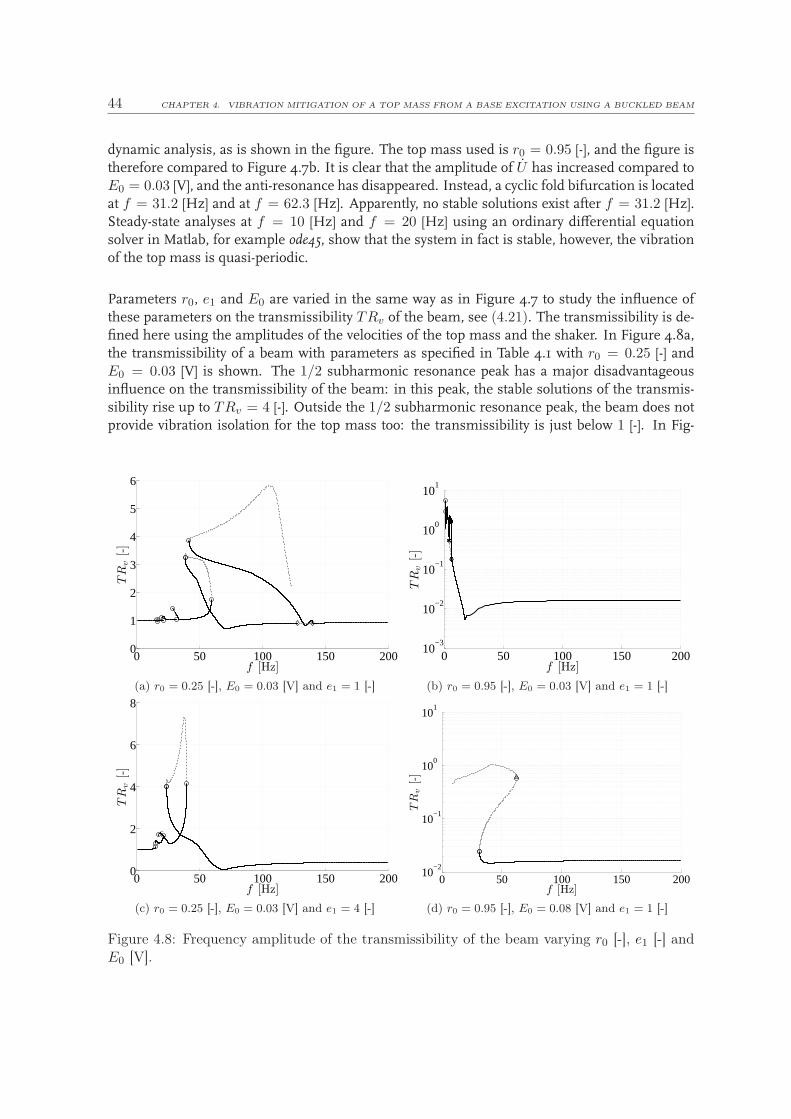
44 CHAPTER 4. VIBRATION MITIGATION OF A TOP MASS FROM A BASE EXCITATION USING A BUCKLED BEAM
dynamic analysis, as is shown in the figure. The top mass used is r0 = 0.95 [-], and the figure istherefore compared to Figure 4.7b. It is clear that the amplitude of U has increased compared toE0 = 0.03 [V], and the anti-resonance has disappeared. Instead, a cyclic fold bifurcation is locatedat f = 31.2 [Hz] and at f = 62.3 [Hz]. Apparently, no stable solutions exist after f = 31.2 [Hz].Steady-state analyses at f = 10 [Hz] and f = 20 [Hz] using an ordinary differential equationsolver in Matlab, for example ode45, show that the system in fact is stable, however, the vibrationof the top mass is quasi-periodic.
Parameters r0, e1 and E0 are varied in the same way as in Figure 4.7 to study the influence ofthese parameters on the transmissibility TRv of the beam, see (4.21). The transmissibility is de-fined here using the amplitudes of the velocities of the top mass and the shaker. In Figure 4.8a,the transmissibility of a beam with parameters as specified in Table 4.1 with r0 = 0.25 [-] andE0 = 0.03 [V] is shown. The 1/2 subharmonic resonance peak has a major disadvantageousinfluence on the transmissibility of the beam: in this peak, the stable solutions of the transmis-sibility rise up to TRv = 4 [-]. Outside the 1/2 subharmonic resonance peak, the beam does notprovide vibration isolation for the top mass too: the transmissibility is just below 1 [-]. In Fig-
0 50 100 150 2000
1
2
3
4
5
6
f [Hz]
TR
v[-]
(a) r0 = 0.25 [-], E0 = 0.03 [V] and e1 = 1 [-]
0 50 100 150 20010
−3
10−2
10−1
100
101
f [Hz]
TR
v[-]
(b) r0 = 0.95 [-], E0 = 0.03 [V] and e1 = 1 [-]
0 50 100 150 2000
2
4
6
8
f [Hz]
TR
v[-]
(c) r0 = 0.25 [-], E0 = 0.03 [V] and e1 = 4 [-]
0 50 100 150 20010
−2
10−1
100
101
f [Hz]
TR
v[-]
(d) r0 = 0.95 [-], E0 = 0.08 [V] and e1 = 1 [-]
Figure 4.8: Frequency amplitude of the transmissibility of the beam varying r0 [-], e1 [-] andE0 [V].

4.4. ANALYSIS OF VIBRATION MITIGATION USING NON-LINEAR STEADY-STATE DYNAMICS 45
ure 4.8b, where the top mass is increased to r0 = 0.95 [-], the beam does show a very satisfactoryvibration reduction. Note that in this figure, a log-scale is used for the y-axis to capture the com-plete picture. In the frequency range f = [50, 200] [Hz], the transmissibility is almost constantat TRv = 0.015 [-]. At f = 22.7 [Hz], the anti-resonance is visible and for lower frequencies TRv
increases rapidly. From this figure, it follows that the beam serves as a very satisfying vibrationisolator for frequencies higher than f = 22.7 [Hz]: only 1 − 2% of the amplitude of the shakermass is transmitted to the top mass. Recall, however, that the influence of higher beam modes isnot taken into account. The experimental results are discussed in Chapter 5, and the conclusionwill be drawn that these higher modes do not have a significant influence on the transmissibilityfor the beam length considered here, i.e L = 0.18 [m]. Third, in Figure 4.8c the transmissibilityof a beam with top mass r0 = 0.25 [-] and imperfection parameter e1 = 4 [-] is shown. Clearly, thetransmissibility has improved significantly with respect to Figure 4.8a with e1 = 1 [-], especiallydue to the vanishing of the 1/2 subharmonic resonance peak: however, the overall transmissibil-ity of TRv = 0.4 [-], which is reached for frequencies f > 50 [Hz] is still relatively high. Lastly,the transmissibility of a beam with r0 = 0.95 and E0 = 0.08 [V] is shown in Figure 4.8d. Again,a log-scale is used for the y-axis. For frequencies f > 50 [Hz], the transmissibility of the beam iscomparable to Figure 4.8b.
Special attention is paid to the changes when the beam length is varied. As observed in Sec-tion 4.3.3, increase of the beam length L can lead to both a decrease and an increase in the trans-missibility of the beam, depending on the topmass applied. Therefore, for a topmass ofmt = 0.9[kg], the beam length is varied between L = [0.18 : 0.03 : 0.360.38] [m]; the relative top mass for
0
100
2000.18 0.2 0.22 0.24 0.26 0.28 0.3 0.32 0.34 0.36 0.38
0
0.2
0.4
0.6
0.8
1
1.2
1.4
1.6
1.8
2
L [m]f [Hz]
TR
v[-]
Figure 4.9: Transmissibility for various beam lengths L, mt = 0.9 [kg].

46 CHAPTER 4. VIBRATION MITIGATION OF A TOP MASS FROM A BASE EXCITATION USING A BUCKLED BEAM
Table 4.2: The transmissibility for various beam length at a frequency f = 200 [Hz].
Length [m] 0.18 0.21 0.24 0.27 0.3 0.33 0.36 0.38r0 [-] 0.22 0.30 0.39 0.50 0.61 0.74 0.88 0.98
TRv [-] 0.925 0.945 0.952 0.952 0.942 0.906 0.722 0.0854
L = 0.38 [m] and mt = 0.9 [kg] is r0 = 0.98 [-]. The resulting frequency-amplitude plot for thetransmissibility is shown in Figure 4.9. The transmissibility for each length at f = 200 [Hz] isalso shown in Table 4.2, together with the corresponding relative top mass r0. From the figureand the table, it follows that a beam with length L = 0.18 [m] has a smaller transmissibility thanthe beams with length L = 0.21 till L = 0.3 [m]. Only beams with a relative top mass r0 > 0.7 [-]have a more satisfying isolating functioning than the shortest beam. For L = 0.38 [m], the trans-missibility is very low, namely TRv = 0.0854. These results correspond to the experiences foundin Section 4.3.4 and shown in Figure 4.3.4.
In Appendix D the gradual change in the frequency-amplitude plots during variation of a beamparameter is found.
In the analysis of the influence of the beam parameters on the transmissibility of the beam, theinfluence of the damping parameters is not discussed. In [14] the conclusion was drawn that thedamping parameters c1 and cq,1 have an influence on the location of the cyclic fold bifurcations,and thus on the length of the harmonic and 1/2 subharmonic resonance peaks. They do not havea major influence on U , and thus TRv, outside these peaks.
4.4.3 Validation optimized beam
In Section 4.3.5, the constraints to find a proper beam to isolate a top mass from a vibrationhave been introduced, based on the linearized system. This is put to the test by comparing asimulation of an optimal beam geometry with simulations based on slight variations around theoptimized beam length and corresponding top mass. The next chapter discusses experimentalresults, and therefore an excitation amplitude, frequency range, and top mass are used that canbe used in the experimental set-up. Considering the limitations of the shaker, the vibration rangeis set between fmin = 40 [Hz] and fmax = 200 [Hz]. Furthermore, the excitation amplitude is setto E0 = 0.03 [V]. As it is easier to vary the top mass during experiments than to vary the beamlength, the ideal top mass that can be isolated with a beam of length L = 0.18 [m] is found usingthe constraints, and mt = 3.629 [kg], corresponding to a relative top mass of r0 = 0.98 [-]. Thesystem parameters are found in Table 4.1. In Figure 4.10a, the transmissibility of the beam withlength L = 0.18 [m] and top mass mt = 3.629 [kg] is shown by the solid thick black line. Twovariations in the top mass are applied, namely mtv1
= mt− 0.01 [kg] and mtv2= mt + 0.01 [kg],
and two variations in length, Lv1 = L− 0.001 [m] and Lv2 = L + 0.001 [m]. These variations areshown in the figure by the solid, dotted, dashed, and dash-dot thin black lines respectively. Fromthis figure, it follows that using a smaller top mass than the ideal top mass indeed leads to anincrease in transmissibility, and thus a worse vibration reduction. This conclusion is also drawnwhen a smaller beam is used. The use of a longer beam or a heavier top mass with respect tothe ideal situation might seem profitable when considering only the transmissibility. Their draw-

4.4. ANALYSIS OF VIBRATION MITIGATION USING NON-LINEAR STEADY-STATE DYNAMICS 47
0 20 40 60 80 100 120 140 160 180 2000
0.005
0.01
0.015
0.02
f [Hz]
TR
v[-]
L = 0.18, mt = 3.629L = 0.18, mt = 3.619L = 0.18, mt = 3.639L = 0.179, mt = 3.629L = 0.181, mt = 3.629
(a) Transmissibility
0 20 40 60 80 100 120 140 160 180 2000.012
0.014
0.016
0.018
0.02
f [Hz]
max(V
)[m
]
L = 0.18, mt = 3.629L = 0.18, mt = 3.619L = 0.18, mt = 3.639L = 0.179, mt = 3.629L = 0.181, mt = 3.629
(b) Maximum transversal displacement at y = L/2
Figure 4.10: Transmissibility and maximum transversal displacement for the optimal beamand four variations.
backs, however, are shown in Figure 4.10b. In this figure, the maximum transversal displacementhalfway the beam is shown for the ideal beam and the four variations, all represented in the sameway as in Figure 4.10a. Furthermore, the maximum transversal displacements representing theonset of plastic deformation are shown for each variation in beam length, indicated by the hori-zontal lines: the solid line represents the maximum displacement for a beam with L = 0.18 [m],the dotted line represents this for a beam with L = 0.179 [m] and the dash-dot line represents thebeam with L = 0.181 [m]. The ideal beam does not reach the maximum displacement at frequen-cies f > 40 [Hz], and plastic deformation does not occur. Furthermore, the beam with lengthL = 0.181 [m] that seemed to be very profitable in Figure 4.10a bends too much during vibra-tion, and plastic deformation occurs. The use of a slightly heavier top mass than the ideal massresults also in an increase in transversal displacement, although plastic deformation only occursat frequencies f < 50 [Hz]. The maximum transversal displacement in the other two variationsis much smaller than the displacement at which plastic deformation occurs, resulting however ina worse vibration reduction performance with respect to the ideal beam. Lastly, following fromFigure 4.10a, the amplitude of the vibration of the top mass is reduced by more than 2 orders andas the maximum transversal displacement is quite large, snap-through does not occur and thebeam does not become straight during vibrations, and thus large accelerations are avoided.
The conclusion is drawn that the constraints used to find the optimal beam length for a certaintop mass that has to be isolated from a vibration with a certain maximum excitation amplitude E0
and for a certain range of excitation frequencies as proposed in 4.3.5 functions well. However, itshould be noted that during the optimization and simulations only N = 1 is used with a 3rd orderTaylor series approximation for (3.12) and (3.14). A 13th order Taylor series approximation wouldgive a more accurate result. This, however, also leads to such elaborate equations of motion that itwould take a lot of computational effort to find the optimal beam the complies with the constraintsset in Section 4.3.5.

48 CHAPTER 4. VIBRATION MITIGATION OF A TOP MASS FROM A BASE EXCITATION USING A BUCKLED BEAM
4.5 Comparison with coil spring
To compare the vibration reduction performance of a buckled beam to that of a standard linear coilspring, the transmissibility of a beam with L = 0.18 [m] and an applied top mass mt = 3.87 [kg](corresponding to r0 = 0.95) is compared to a coil spring. The system parameters of the beamare found in Table 4.1. The eigenfrequency of the coil spring is taken identical to the eigenfre-quency of the linearized buckled beam and this results in a desired stiffness of the coil springof kcs = 1.3138 · 104 [N/m]. Figure 4.11a shows the transmissibility of the buckled beam over afrequency range of [1 200] [Hz]. It follows that the transmissibility of the buckled beam is smallerfor frequencies between 10 < f < 45 [Hz]. For higher frequencies, the transmissibility of thecoil springs keeps decreasing, while the transmissibility of the buckled beam remains constantat TR = 0.01 [-]. It must be noted however, that internal modes worsen the transmissibility ofthe coil spring as described in [31], and that these modes are not modeled here, because in Fig-ure 4.11b the coil spring is assumed to be massless.
To compare the dimensions of the buckled beam with the dimensions of a possible coil springwith stiffness kcs = 1.3138·104 [N/m], the following four relations are used to find an appropriategeometry for the coil spring [30]
kcs =Gd4
8D3n, (4.28)
f1 =
√
Gg
32ρ
2d
πD2n, (4.29)
τ =δGd
nπD2Kw, (4.30)
and
mcs =1
4π2d2nDρ, (4.31)
with G the shear modulus, D the coil diameter, d the wire diameter, n the number of coils, f1
the lowest internal eigenfrequency of the coil spring with both ends fixed, τ the ‘corrected’ shearstress, and mcs the mass of the spring. Kw is a force-independent correction factor for the shearstress [30], Kw = 4c−1
4c−4 + 0.615c , with c = D
d the spring index. Furthermore, δ is the total deflection
of the top mass in static equilibrium. Using mtg = kcsδ, δ = 1.3138·104
3.87·9.81 = 2.89 · 10−3 [m]. Itis noted that (4.28) till (4.31) hold for imperial units and, therefore, metric units (as used here)should be first converted before substituting them into these equations. The shear modulus forsteel is typically G = 79.3 · 109 [N/m2] [30]. The length of the coil spring is assumed to be
Lcs = n(d + δc + 2usmax/n), (4.32)
with δc = δn the deflection per coil, and the maximum shaker table amplitude amplified by 2 as
a safety factor. The maximum shaker table amplitude for f = [1, 200] [Hz] and E0 = 0.03 [V] isusmax = 9.86 ·10−4 [m]. It is desired to have an internal eigenfrequency that lies above the secondeigenfrequency of the buckled beam system, which is 180 [Hz], see Figure 3.10, i.e. f1 > 180 [Hz].Furthermore, the following demands are set: the length of the coil spring should not exceed the

4.6. SUMMARY 49
0 50 100 150 20010
−4
10−2
100
102
f [Hz]
TR
v[-]
(a) Transmissibility of buckled beam
0 50 100 150 20010
−4
10−2
100
102
104
f [Hz]
TR
v[-]
(b) Transmissibility of coil spring
Figure 4.11: The transmissibility of a buckled beam and a coil spring, mt = 3.87 [kg], E0 =0.03 [V].
length of the buckled beam, the mass of the coil spring is not heavier than 0.1 [kg] (the mass ofthe beam is mb = 0.0106 [kg]), and the number of coils is at least 5 in order to be considered asa coil spring. Moreover,the shear stress must be smaller than the yield shear stress. Accordingto Tresca’s criterion [9], the absolute maximum shear stress is equal to the absolute maximumshear stress at the yield point in a simple tension test. The absolute maximum shear stress in asimple uni-axial tension with an applied stress of σ is [9] σ/2. The maximum shear stress yieldcriterion is thus τmax = σy/2, with σy = 4.6·108 [N/m2]. A feasible coil spring that complies withthese demands, has for instance the following dimensions: d = 0.0045 [m] and D = 0.037 [m],such that Lcs = 0.0299 [m], n = 6, mcs = 0.0873 [kg], and f1 = 196 [Hz]. The shear stressin the coil spring is τ = 6.32 · 107 [N/m2], which is about 27% of the maximum shear stress.Analyses of the fatigue limit show that fatigue does not play a role in the use of this spring.The preliminary conclusion is drawn that for this particular case, the coil spring does not seemto perform worse than the buckled beam. It still must be mentioned, however, that the modaldensity of longitudinal modes of coil springs in general is much higher than the modal density ofbuckled beams, as can also be seen from Figure 2.3. Further study is needed to be able to makea fair comparison between the buckled beam and coil spring, based on their vibration mitigationand non-linear dynamic steady-state behavior.
4.6 Summary
In this chapter, first the complete semi-analytical model of the base-excited buckled beam hasbeen derived including the equations of motion of the shaker-amplifier combination, after whichit was linearized around the static equilibrium. Subsequently, the vibration reduction perfor-mance of the buckled beam was discussed using this linearized semi-analytical model. Beam pa-rameters such as the length and the initial imperfection parameter, and the top mass that has tobe isolated were varied and their influence on the transmissibility were discussed. Furthermore,constraints of the buckled beam during vibration considering among others plastic deformationwere derived and used to derive the optimal beam length that can be used to isolate a top mass

50 CHAPTER 4. VIBRATION MITIGATION OF A TOP MASS FROM A BASE EXCITATION USING A BUCKLED BEAM
from base vibrations within a certain range of excitation frequencies and for certain excitationamplitudes. Then, the non-linear dynamic steady-state response of a beam with top mass was in-vestigated, and the influence of the beam length, initial imperfection, excitation amplitude, andtop mass itself on the transmissibility was discussed. The constraints used to find the optimalbeam length given values for the top mass and the imperfection are verified using this dynamicanalysis. It appears that these constraint provide a good guideline to find the ideal length. Lastly,the transmissibility of a buckled beam was compared to that of a linear coil spring, and it followsthat for the particular case considered, the coil spring does not perform worse than the buckledbeam.

Chapter 5
Experimental results and model
validation
To validate the semi-analytical model that has been derived in Chapter 4, experimental frequencysweep results are compared to semi-analytical results. Two sets of experiments are conducted, inwhich the beam length is varied, and for each beam length, various top masses are considered.The results from the semi-analytical model are compared to the experimental results for eachbeam, and the transmissibility of both beams is discussed. This chapter starts by explainingthe experimental approach. In Section 5.2, a beam with length L = 0.183 [m] is analyzed. InSection 5.3, a beam with length L = 0.366 [m] is analyzed.
5.1 Frequency sweeps
During one experiment, a frequency sweep down is carried out, which is followed by a frequencysweep up, to investigate the steady-state behavior of the system. The start frequency of the har-monic input voltage of the amplifier E(t) is set to f = 200 [Hz], after which the frequency isdecreased with step size ∆f = 1 [Hz] until the minimum frequency fmin is reached. The excita-tion frequency is then increased again with ∆f = 1 [Hz] up to f = 200 [Hz]. For each frequency,the number of excitation periods is set to Np = 150, and it is assumed that after 100 excitationperiods a steady-state periodic solution is reached. Thus, the results of the experiments are basedon the last 50 periods of the vibration for each excitation frequency. Each experiment is repeatedat least twice. The experimental results discussed in this chapter are the average of the repeatedexperiments, to reduce the influence of small disturbances.
5.2 Experimental results L = 0.183 [m]
The experimental results of a steel beam with length L = 0.183 [m] are discussed in this section.The parameter values used to model the beam are shown in Table 5.1. The values for the beam’sdimensions (i.e. L, b, and h) are obtained bymeasuring. Also, the initial geometrical imperfectione1 is obtained by measuring, and observation shows that the beam is initially shaped accordingto the first mode shape as derived in (3.7). The values for the damping parameters c1 and cq,1 are
51
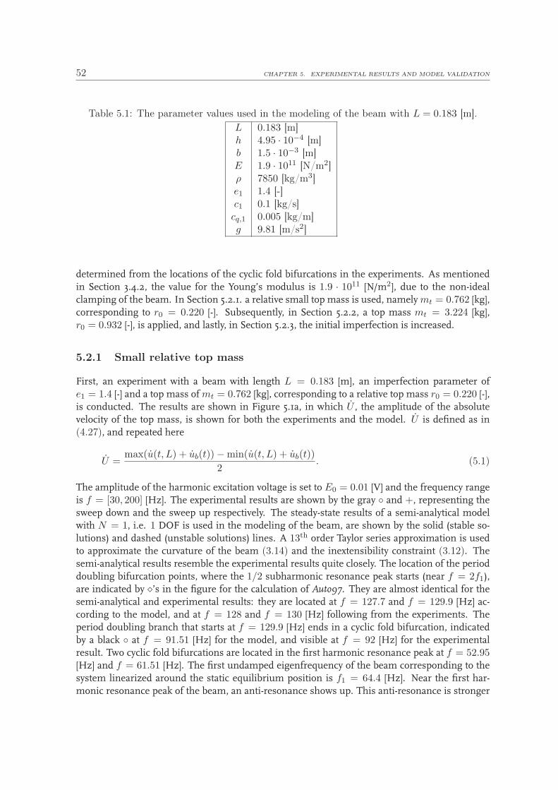
52 CHAPTER 5. EXPERIMENTAL RESULTS AND MODEL VALIDATION
Table 5.1: The parameter values used in the modeling of the beam with L = 0.183 [m].
L 0.183 [m]h 4.95 · 10−4 [m]b 1.5 · 10−3 [m]E 1.9 · 1011 [N/m2]ρ 7850 [kg/m3]e1 1.4 [-]c1 0.1 [kg/s]cq,1 0.005 [kg/m]g 9.81 [m/s2]
determined from the locations of the cyclic fold bifurcations in the experiments. As mentionedin Section 3.4.2, the value for the Young’s modulus is 1.9 · 1011 [N/m2], due to the non-idealclamping of the beam. In Section 5.2.1. a relative small top mass is used, namely mt = 0.762 [kg],corresponding to r0 = 0.220 [-]. Subsequently, in Section 5.2.2, a top mass mt = 3.224 [kg],r0 = 0.932 [-], is applied, and lastly, in Section 5.2.3, the initial imperfection is increased.
5.2.1 Small relative top mass
First, an experiment with a beam with length L = 0.183 [m], an imperfection parameter ofe1 = 1.4 [-] and a top mass of mt = 0.762 [kg], corresponding to a relative top mass r0 = 0.220 [-],is conducted. The results are shown in Figure 5.1a, in which U , the amplitude of the absolutevelocity of the top mass, is shown for both the experiments and the model. U is defined as in(4.27), and repeated here
U =max(u(t, L) + ub(t))−min(u(t, L) + ub(t))
2. (5.1)
The amplitude of the harmonic excitation voltage is set to E0 = 0.01 [V] and the frequency rangeis f = [30, 200] [Hz]. The experimental results are shown by the gray and +, representing thesweep down and the sweep up respectively. The steady-state results of a semi-analytical modelwith N = 1, i.e. 1 DOF is used in the modeling of the beam, are shown by the solid (stable so-lutions) and dashed (unstable solutions) lines. A 13th order Taylor series approximation is usedto approximate the curvature of the beam (3.14) and the inextensibility constraint (3.12). Thesemi-analytical results resemble the experimental results quite closely. The location of the perioddoubling bifurcation points, where the 1/2 subharmonic resonance peak starts (near f = 2f1),are indicated by ⋄’s in the figure for the calculation of Auto97. They are almost identical for thesemi-analytical and experimental results: they are located at f = 127.7 and f = 129.9 [Hz] ac-cording to the model, and at f = 128 and f = 130 [Hz] following from the experiments. Theperiod doubling branch that starts at f = 129.9 [Hz] ends in a cyclic fold bifurcation, indicatedby a black at f = 91.51 [Hz] for the model, and visible at f = 92 [Hz] for the experimentalresult. Two cyclic fold bifurcations are located in the first harmonic resonance peak at f = 52.95[Hz] and f = 61.51 [Hz]. The first undamped eigenfrequency of the beam corresponding to thesystem linearized around the static equilibrium position is f1 = 64.4 [Hz]. Near the first har-monic resonance peak of the beam, an anti-resonance shows up. This anti-resonance is stronger

5.2. EXPERIMENTAL RESULTS L = 0.183 [M] 53
0 50 100 150 20010
−3
10−2
10−1
f [Hz]
U[m
/s]
sweep upsweep downstableunstable
(a) Amplitude of velocity of top mass
0 50 100 150 2000
0.2
0.4
0.6
0.8
1
1.2
1.4
1.6
1.8
2
f [Hz]T
Rv
[-]
sweep upsweep downstableunstable
(b) Transmissibility
Figure 5.1: Comparison between model and experiments for a beam with L = 0.183 [m] andtop mass mt = 0.762 [kg], E0 = 0.01 [V].
in the semi-analytical model than in experiments. For frequencies below 50 [Hz], the experimen-tal and semi-analytical results deviate slightly. At f ≈ 190 [Hz], the second harmonic resonancefrequency of the beam is visible in the experimental results. It is important to observe that thesemi-analytical model with N = 1 apparently accurately describes the behavior in this frequencyrange. The second harmonic resonance peak near f = 190 [Hz] has only minor influence.
The transmissibility TRv of the beam is defined similar to (4.21), but now using the axial veloci-ties of the top mass and the shaker:
TRv =max(u(t, L) + us(t))−min(u(t, L) + us(t))
max(us(t))−min(us(t)), (5.2)
and is plotted in Figure 5.1b. From this figure, it follows that the beam barely provides anyisolation for the current top mass, as expected for low r0. Especially in the 1/2 subharmonic peakand in the first harmonic resonance peak, the transmissibility increases rapidly, and even exceeds1, indicating that the shaker table vibration level in fact is lower than the vibration level of thetop mass. The shape of the transmissibility of the beam is more irregular than the shape of theamplitude of the velocity of the top mass, and the semi-analytical results and the experiments donot correspond as much as in Figure 5.1a. This is due to the fact that in order to obtain TRv,two laser signals are used. The signal from the laser used to measure the velocity of the shakeris less smooth than the signal from the laser used to measure the velocity of the top mass. Thisshows up especially in the transmissibility, as both signals are added and dived here, and the non-smoothness of a signal is enhanced, which holds also for the error between the semi-analyticalmodel and the experiments. To illustrate the difference in laser signal, part of the time signalobtained from both lasers are shown in Appendix G.

54 CHAPTER 5. EXPERIMENTAL RESULTS AND MODEL VALIDATION
5.2.2 Large relative top mass
Subsequently, a top mass of mt = 3.224 [kg] is mounted on the beam with length L = 0.183 [m],which corresponds to a relative top mass of r0 = 0.932 [-]. For validation of the semi-analyticalmodel, the experimental results are compared to results from the semi-analytical model usingN = 1 and 13th order Taylor series approximations. The amplitude of the harmonic excitationvoltage is again set to E0 = 0.01 [V] and the frequency range is f = [20, 200] [Hz]. First, thetransmissibility of the beam is discussed. Then, to check whether plastic deformation mighthave occurred during the frequency sweeps, the semi-analytical model is used to compare themaximum transversal displacement halfway the length of the beam occurring during the fre-quency sweeps to the transversal displacement at the onset of plastic deformation. Furthermore,static analyses of this beam are compared to FEA.
Transmissibility
The amplitude of the velocity of the top mass U is shown in Figure 5.2a. The experimental resultsare again indicated by the gray and+marks. The stable harmonic solution of the semi-analyticalmodel is indicated by the solid black line. For this topmass, no unstable solutions are predicted bythe semi-analytical model. The conclusion is drawn that the semi-analytical model resembles theexperimental results using the parameter values as defined in Table 5.1 especially for f < 50 [Hz].For higher frequencies, the relative difference between the experimental and semi-analytical re-sults is approximately 30%. According to the semi-analytical model, after linearization aroundthe static equilibrium position, the first undamped eigenfrequency of the beam is f1 = 2.84 [Hz].In the experimental results, at f ≈ 152 [Hz] the second harmonic resonance peak of the beam isvisible. As only 1 mode is taken into account for the beam in the simulations, the resonance due
0 50 100 150 20010
−5
10−4
10−3
f [Hz]
U[m
/s]
sweep upsweep downstable
(a) Amplitude of velocity of top mass
0 50 100 150 2000
0.005
0.01
0.015
0.02
0.025
0.03
f [Hz]
TR
v[-]
sweep upsweep downstable
(b) Transmissibility
Figure 5.2: Comparison between model and experiments for a beam with L = 0.183 [m] andtop mass mt = 3.224 [kg], E0 = 0.01 [V].

5.2. EXPERIMENTAL RESULTS L = 0.183 [M] 55
to the second mode obviously is not present in the semi-analytical results. In Appendix F, thesemi-analytical model is extended with a 2nd and a 3rd beam mode (N = 2, 3). In these analyses,the Taylor series approximation for the beam curvature and inextensibility constraint cannot beof higher order than 7 and 3 for the two higher modes respectively, due to limitations of MAPLE,the package used to define the equations of motion. This can result in quite unreliable outcomesfor semi-analytical models with N > 1. Furthermore, in Section 3.5, the conclusion has beendrawn that the eigenfrequencies of the higher modes deviate much from the FEA.
Following from the experimental results presented in Figure 5.2b, the transmissibility of the beamlies between TRv = 0.01 and TRv = 0.015 [-] for 50 < f < 150 [Hz]. This means that only 1%of the velocity amplitude of the shaker table is transmitted to the top mass, which is a good resultregarding vibrationmitigation. The transmissibility computed by the semi-analytical model usingN = 1 is about 20% higher than the experimental results. In conclusion, the influence of thesecond beam mode is limited and the semi-analytical model using N = 1 has good predictivevalue for the frequency range of interest. Both the experimental results for U and TRv are a bitirregular. This is due to the fact that the top mass only moves very slightly, and the resolutionof the laser signal is reached. The minimum velocity that can be detected by the laser used tomeasure the velocity of the top mass is approximately 3 · 10−5 [m/s], the minimum velocity thatcan be detected by the other laser is approximately 3 · 10−4 [m/s]. Again, time signals of bothlasers are included in Appendix G.
Checking for plasticity and snap-through
In Figure 5.3a, the maximum value of the total transversal displacement V at position y = L/2 isshown for the frequency range of interest. A maximum transversal displacement ofv(L/2) = 0.01088 [m] occurs at f = 17.07 [Hz]. This total transversal displacement is defined as
V (L/2) = v0(L/2) + v(t, L/2). (5.3)
0 50 100 150 2000.0095
0.01
0.0105
0.011
f [Hz]
max(V
)[m
]
(a) Maximum total transversal displacement
0 50 100 150 2008
8.5
9
9.5
10x 10−3
f [Hz]
min
(V)
[m]
(b) Minimum total transversal displacement
Figure 5.3: Maximum and minimum total transversal displacement for a beam with L = 0.183[m] and top mass mt = 3.224 [kg], E0 = 0.01 [V].
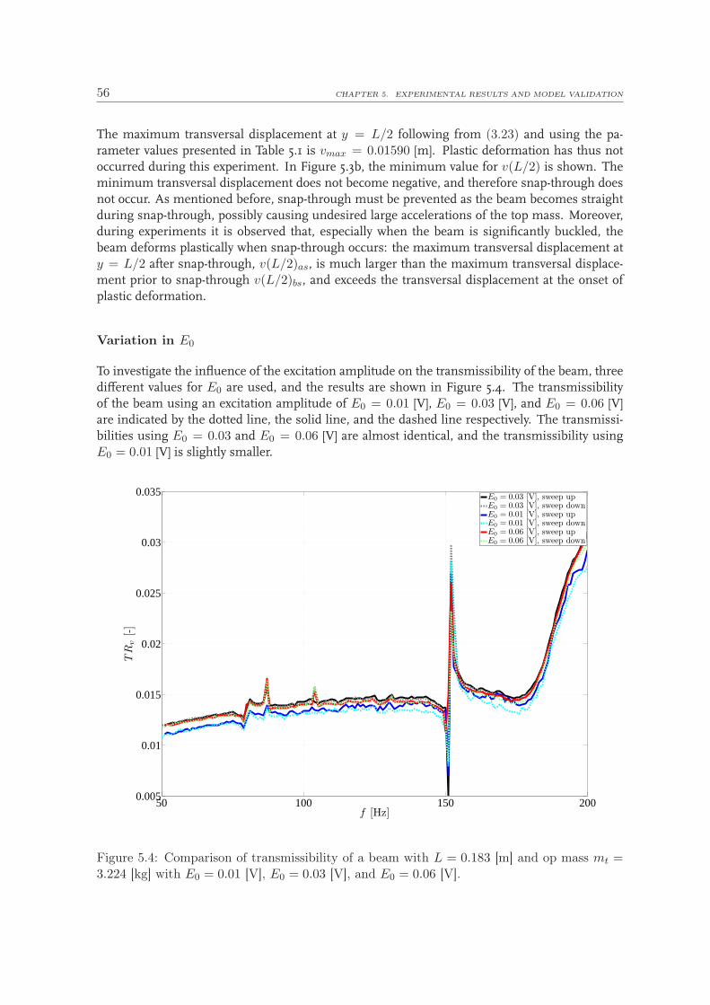
56 CHAPTER 5. EXPERIMENTAL RESULTS AND MODEL VALIDATION
The maximum transversal displacement at y = L/2 following from (3.23) and using the pa-rameter values presented in Table 5.1 is vmax = 0.01590 [m]. Plastic deformation has thus notoccurred during this experiment. In Figure 5.3b, the minimum value for v(L/2) is shown. Theminimum transversal displacement does not become negative, and therefore snap-through doesnot occur. As mentioned before, snap-through must be prevented as the beam becomes straightduring snap-through, possibly causing undesired large accelerations of the top mass. Moreover,during experiments it is observed that, especially when the beam is significantly buckled, thebeam deforms plastically when snap-through occurs: the maximum transversal displacement aty = L/2 after snap-through, v(L/2)as, is much larger than the maximum transversal displace-ment prior to snap-through v(L/2)bs, and exceeds the transversal displacement at the onset ofplastic deformation.
Variation in E0
To investigate the influence of the excitation amplitude on the transmissibility of the beam, threedifferent values for E0 are used, and the results are shown in Figure 5.4. The transmissibilityof the beam using an excitation amplitude of E0 = 0.01 [V], E0 = 0.03 [V], and E0 = 0.06 [V]are indicated by the dotted line, the solid line, and the dashed line respectively. The transmissi-bilities using E0 = 0.03 and E0 = 0.06 [V] are almost identical, and the transmissibility usingE0 = 0.01 [V] is slightly smaller.
50 100 150 2000.005
0.01
0.015
0.02
0.025
0.03
0.035
f [Hz]
TR
v[-]
E0 = 0.03 [V], sweep upE0 = 0.03 [V], sweep downE0 = 0.01 [V], sweep upE0 = 0.01 [V], sweep downE0 = 0.06 [V], sweep upE0 = 0.06 [V], sweep down
Figure 5.4: Comparison of transmissibility of a beam with L = 0.183 [m] and op mass mt =3.224 [kg] with E0 = 0.01 [V], E0 = 0.03 [V], and E0 = 0.06 [V].

5.2. EXPERIMENTAL RESULTS L = 0.183 [M] 57
5.2.3 Transmissibility with large initial imperfection using plasticity
In Section 4.3.3, the conclusion has been drawn that an increasing initial imperfection leads to animprovement in vibration mitigation: even relative small top masses can be isolated significantlyin this way, in theory. Therefore, two experiments are conducted, in which the imperfection isvaried. An initial geometrical imperfection can be realized in several ways. For instance, thebeam can be shaped during manufacturing, or a magnet can be used to force the beam to bendin one direction. Here, the imperfection is realized by pre-bending (buckling) of the beam suchthat the beam deforms plastically.
In Section 5.2.1, the experiment with a beam with an imperfection parameter of e1 = 1.4 [-] anda top mass of mt = 0.762 [kg], corresponding to r0 = 0.214 [-] has been discussed. The con-clusion was drawn that hardly any vibration reduction is obtained. Now an axial displacementof u(L) = 27.5 · 10−3 [m] is prescribed for one end of the beam. The other end of the beam isclamped, and therefore the beam buckles and deforms plastically in a shape closely resemblingthe first mode shape (3.10). After unloading, an initial imperfection of e1 = 5 [-] results. Theassumption is made that the material properties have not changed and that effects such as strainhardening do not occur. The excitation amplitude is again set to E0 = 0.01 [V] and the frequencyrange is f = [50, 200] [Hz]. The resulting amplitude of the top mass is shown in Figure 5.5a forthe experiments as well as for the semi-analytical model for N = 1. A remarkably good corre-spondence is obtained. The 1/2 subharmonic resonance peak from Figure 5.1a has disappeared.This in particular results in a major improvement in vibration reduction, see Figure 5.5b. As thematerial properties will change and prestress is introduced when plastic deformation occurs, it isrecommended to consider modeling plastic deformation in future research of vibration mitiga-tion based on buckled beams.
0 50 100 150 20010
−4
10−3
10−2
10−1
100
f [Hz]
U[m
/s]
sweep upsweep downstableunstable
(a) Amplitude of velocity of top mass
50 100 150 2000
0.1
0.2
0.3
0.4
0.5
0.6
0.7
0.8
0.9
1
f [Hz]
TR
v[-]
sweep upsweep downstable
(b) Transmissibility
Figure 5.5: Comparison between model and experiments for a beam with L = 0.183 [m] witha large initial imperfection (e1 = 5 [-]), top mass mt = 0.762 [kg], and E0 = 0.01 [V].

58 CHAPTER 5. EXPERIMENTAL RESULTS AND MODEL VALIDATION
Table 5.2: Comparison of static analysis of semi-analytical model with N = 1 and FEA forL = 0.183 [m], and various values for e1 and mt.
e1 = 1.4, mt = 0.762 [kg] e1 = 1.4, mt = 3.224 [kg] e1 = 5.0, mt = 0.762 [kg]
N = 1v(L/2) [m] 1.956 · 10−4 8.934 · 10−3 6.988 · 10−4
u(L) [m] −4.172 · 10−6 −1.25 · 10−3 −5.324 · 10−5
f1 [Hz] 63.85 2.867 43.45
FEAv(L/2) [m] 1.938 · 10−4 9.132 · 10−3 7.049 · 10−4
u(L) [m] −5.148 · 10−6 −1.305 · 10−3 −5.473 · 10−5
f1 [Hz] 62.93 2.789 43.09
5.2.4 Comparison between static semi-analytical and FEA results
In Section 3.3.1, the conclusion has been drawn that for increasing topmass, the static response ofthe semi-analytical model deviates more from the FEM-model than for relative small top masses.Therefore, to further validate the results of the semi-analytical model of the beam with N = 1and a 13th order Taylor series approximation, a static and modal FEA is performed on a beamwith parameter values as defined in Table 5.1. For the FEA, the beam is modeled in the sameway as in Section 3.3, using 52 elements as the beam is slightly larger than the one modeled inSection 3.3. The static and modal FEA results are compared with the static and modal analysisresults obtained from the semi-analytical model with N = 1. The static transversal displacementv(L/2) halfway the length of the beam, and the relative axial displacement of the top mass u(L)are shown in Table 5.2 for the situations of the three experiments discussed above and for boththe semi-analytical model and the FEA. The first eigenfrequency f1 of the beam obtained fromboth analysis methods after linearization around the static equilibrium position is shown in thistable too.
0 1 2x 10
−4
0
0.04575
0.0915
0.1372
0.183
v(L/2) [m]
y[m
]
1-DOF SAFEA
(a) e1 = 1.4 [-], mt = 0.762 [kg]
0 5 10x 10
−3
0
0.0457
0.0915
0.1372
0.183
v(L/2) [m]
y[m
]
1-DOF SAFEA
(b) e1 = 1.4 [-], mt = 3.224 [kg]
0 2 4 6x 10
−4
0
0.0457
0.0915
0.1372
0.183
v(L/2) [m]
y[m
]
1-DOF SAFEA
(c) e1 = 5.0 [-], mt = 0.762 [kg]
Figure 5.6: The static transversal displacement v(y) along the beam of the three experiments.

5.3. EXPERIMENTAL RESULTS L = 0.366 [M] 59
The conclusion is drawn that the axial displacement of the top mass obtained from the semi-analytical model differs only a few percent from the FEA results, except for the axial displacementfor mt = 0.762 [kg] and e1 = 1.4 [-]. This, however, has already been explained in Section 3.3.Furthermore, the maximum transversal displacement v(L/2) occurring during the experimentwith mt = 3.224 [kg] obtained from the semi-analytical model is accurate, assuming that theFEA results closely resemble reality. Lastly, the first eigenfrequency of the beam obtained afterlinearization around the static equilibrium position corresponds to the first eigenfrequency of thebeam obtained from FEA. In Figure 5.6, for each of the three static analyses the static transversaldisplacement v(y) along the beam is plotted for the semi-analytical model (N = 1, 13th order)and the FEA. Clearly, the results from the semi-analytical model resemble the FEA results.
5.3 Experimental results L = 0.366 [m]
This section discusses the comparison between the results of the semi-analytical model, and theexperimental results when the beam length is doubled to L = 0.366 [m]. Depending on the topmass used, use is made of 1 or 3 modes to model the beam. Two top masses are used, namelymt = 0.509 [kg] and mt = 0.785 [kg]. The beam parameters used in the semi-analytical modelare listed in Table 5.3. Simulations show that E = 1.75 · 1011 [N/m2] leads to a more satisfactoryresemblance of the semi-analytical model to the experiments. Note that this is a remarkably lowvalue for this parameter. The value of c1 is adjusted to the location of the cyclic fold bifurcation.
In order to be able to mount the long beam into the set-up, the support on which the shaker ismounted is improved such that it can be altered in height. After this adaptation, the shaker pa-rameters are identified again as explained in Appendix C. It appeared that the shaker parametersare slightly changed after the adaptation, and they are included in Appendix C.
5.3.1 Small relative top mass
A top mass of mt = 0.509 [kg] is applied, corresponding to a relative top mass r0 = 0.621 [-]. Theexcitation amplitude is set to E0 = 0.005 [V] and the frequency range is set to f = [13, 250] [Hz].In Figure 5.7, U is shown for both the experiments and the semi-analytical model using N = 1and a 13th order Taylor series approximation. The experimental results are indicated again by
Table 5.3: The parameter values used in the modeling of the beam with L = 0.366 [m].
L 0.366 [m]h 4.95 · 10−4 [m]b 1.5 · 10−3 [m]E 1.75 · 1011 [N/m2]ρ 7850 [kg/m3]e1 2.4 [-]c1 0.05 [kg/s]cq,1 0.005 [kg/m]g 9.81 [m/s2]

60 CHAPTER 5. EXPERIMENTAL RESULTS AND MODEL VALIDATION
0 50 100 150 200 25010
−4
10−3
10−2
10−1
f [Hz]
U[m
/s]
sweep upsweep downstableunstable
(a) Amplitude of velocity of top mass
0 50 100 150 200 2500
0.2
0.4
0.6
0.8
1
1.2
1.4
1.6
1.8
2
f [Hz]T
Rv
[-]
sweep upsweep downstableunstable
(b) Transmissibility
Figure 5.7: Comparison between N = 1 SA model and experiments for a beam with L = 0.366[m], top mass mt = 0.509 [kg], and E0 = 0.005 [V].
and +, representing the sweep down and the sweep up respectively. From Figure 5.7, it followsthat the results of the semi-analytical model with the beam parameter values as defined in Ta-ble 5.3 resembles the experimental results quite closely. The period doubling bifurcations, fromwhich the 1/2 subharmonic resonance peak emerges, are located at f ≈ 2f1 = 19.42 [Hz] andf = 21.93 [Hz] for the semi-analytical model, whereas this peak in the experimental results islocated between f = 19 [Hz] and f = 22 [Hz]. The cyclic fold bifurcation in this peak is locatedat f = 15.8 [Hz] for the semi-analytical model, and at f = 16 [Hz] in the experiment. In theexperimental results, the second harmonic resonance of the beam is visible around f = 40 [Hz],its corresponding 1/2 subharmonic resonance is located between f = 61 [Hz] and f = 82 [Hz],the third harmonic resonance of the beam is located around f = 86 [Hz], and the fifth harmonicresonance of the beam is visible around f = 225 [Hz]; the fourth harmonic resonance is notvisible. The locations of the second till fifth harmonic resonances of the beam are compared toresults from FEA. Clearly, the height of the resonance peaks decreases for increasing mode num-ber. In Figure 5.8b, the transmissibility is shown. As expected for a low relatively top mass, thebeam does not provide much vibration reduction for the top mass. Again, the 1/2 subharmonicresonance has a detrimental influence on the transmissibility.
5.3.2 Large relative top mass
The top mass is increased to mt = 0.785 [kg], corresponding to r0 = 0.985, and U and thetransmissibility of the beam are discussed. Subsequently, occurrence of plastic behavior andsnap-through is investigated. The amplitude of the excitation voltage is set to E0 = 0.01 [V] andthe frequency range is set to f = [50, 250] [Hz].

5.3. EXPERIMENTAL RESULTS L = 0.366 [M] 61
Transmissibility
The amplitude of the velocity of the top mass U is shown in Figure 5.8a. Again, the experimentalresults are shown by and +. From this figure, it follows that modeling only the first mode ofthe beam is insufficient, although U from the semi-analytical model (N = 1, 13th order) is ofthe same order as the experimental results outside frequency ranges where resonances occur.The transmissibility of the beam is shown in Figure 5.8b. Again, the transmissibility from thesemi-analytical model is of the same order as the experimental results (besides resonances). Theinfluence of the third and fifth harmonic resonances of the beam on the transmissibility is signif-icant, and the influence of the fourth harmonic resonance to a smaller extent. The experimentalresults in Figure 5.8c show that in the frequency range f = [70, 190] [Hz] (between the third andthe fifth harmonic resonance) the beam does serve as a vibration isolator, i.e. TR < 0.1. Asconcluded earlier, adding a third beam mode to the semi-analytical model can result in inaccu-rate results as the order of Taylor series has to be reduced radically. To illustrate this, U and TRv
from the semi-analytical model with N = 3 using a 3rd order Taylor series approximation areplotted in Figures 5.9a and 5.9b respectively. The damping and imperfection parameters of thetwo additional modes are: e2 = e3 = 0.01 [-], c2 = c3 = 0.1 [kg/s], and cq,2 = cq,3 = 0.1 [kg/m].The results of the semi-analytical model again are of the same order as the experimental results.But the results are obviously not as accurate as the results presented in Figure 5.2, i.e. the shortbeam with large top mass where a semi-analytical model with N = 1 is sufficient. Clearly, themodes higher than N = 3 are not visible in the semi-analytical results, although especially thefifth resonance peak has a significant detrimental influence on the transmissibility. Due to com-putational limitations in MAPLE, the beam cannot be modeled with more than four modes inthe semi-analytical model. As especially the fifth mode still has a detrimental influence on thetransmissibility, it is advisable to improve the semi-analytical modeling such that modes higherthan the fourth mode can be modeled.
0 50 100 150 200 25010
−6
10−5
10−4
10−3
10−2
f [Hz]
U[m
/s]
sweep upsweep downstable
(a) Amplitude of velocity of topmass
0 50 100 150 200 2500
0.05
0.1
0.15
0.2
0.25
0.3
0.35
0.4
0.45
0.5
f [Hz]
TR
v[-]
sweep upsweep downstable
(b) Transmissibility
0 50 100 150 200 2500
0.01
0.02
0.03
0.04
0.05
0.06
0.07
0.08
f [Hz]
TR
v[-]
sweep upsweep downstable
(c) Zoom of transmissibility
Figure 5.8: Comparison between model (N = 1) and experiments for a beam with L = 0.366[m], top mass mt = 0.785 [kg], and E0 = 0.01 [V].
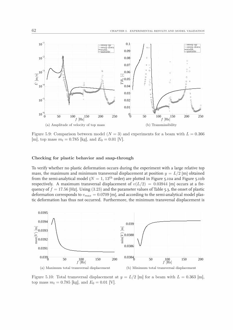
62 CHAPTER 5. EXPERIMENTAL RESULTS AND MODEL VALIDATION
0 50 100 150 200 25010
−6
10−5
10−4
10−3
10−2
10−1
f [Hz]
U[m
/s]
sweep upsweep downstableunstable
(a) Amplitude of velocity of top mass
0 50 100 150 200 2500
0.01
0.02
0.03
0.04
0.05
0.06
0.07
0.08
0.09
0.1
f [Hz]T
Rv
[-]
sweep upsweep downstableunstable
(b) Transmissibility
Figure 5.9: Comparison between model (N = 3) and experiments for a beam with L = 0.366[m], top mass mt = 0.785 [kg], and E0 = 0.01 [V].
Checking for plastic behavior and snap-through
To verify whether no plastic deformation occurs during the experiment with a large relative topmass, the maximum and minimum transversal displacement at position y = L/2 [m] obtainedfrom the semi-analytical model (N = 1, 13th order) are plotted in Figure 5.10a and Figure 5.10brespectively. A maximum transversal displacement of v(L/2) = 0.03944 [m] occurs at a fre-quency of f = 17.56 [Hz]. Using (3.23) and the parameter values of Table 5.3, the onset of plasticdeformation corresponds to vmax = 0.0709 [m], and according to the semi-analytical model plas-tic deformation has thus not occurred. Furthermore, the minimum transversal displacement is
0 50 100 150 2000.039
0.0391
0.0392
0.0393
0.0394
0.0395
f [Hz]
max(V
)[m
]
(a) Maximum total transversal displacement
0 50 100 150 2000.0384
0.0386
0.0388
0.039
f [Hz]
min
(V)
[m]
(b) Minimum total transversal displacement
Figure 5.10: Total transversal displacement at y = L/2 [m] for a beam with L = 0.363 [m],top mass mt = 0.785 [kg], and E0 = 0.01 [V].

5.3. EXPERIMENTAL RESULTS L = 0.366 [M] 63
larger than zero, and therefore snap-through does not occur too. However, only the first mode ofthe beam is taken into account in this analysis. As stated before, Figure 5.8b shows that the thirdand fifth harmonic resonances have a significant influence, and the fourth harmonic resonanceto a smaller extent, on U and the transmissibility, and thus on V (L/2). Because semi-analyticalresults for N > 1 may be inaccurate since the order of the Taylor series approximation cannot betoo high (otherwiseMAPLE fails), it is not possible to check for plasticity forN > 1. Moreover, thecriterion for plasticity given in (3.23) is only valid for N = 1, and should be modified for N > 1.After experimentation, at least no visible evidence was found for plastic deformation. However,in Section 5.3.4 it will be shown that the results from experiments that were conducted after theexperiments with high relative top mass, differ slightly from the first experiments conducted withthe same beam. So, plasticity may have occurred during the experiments.
5.3.3 Comparison between static semi-analytical and FEA results
The static response of the beam with beam parameter values for L, h, b, e1, and E as defined inTable 5.3 is analyzed using a semi-analytical model based on N = 1 and a 13th order Taylor seriesapproximation, a semi-analytical model based on N = 3 and a 3rd order Taylor series approxi-mation, and FEA. The beam is modeled in the same way as in Section 3.3, using 104 elements.The transversal displacement halfway the length of the beam v(L/2), the axial displacement ofthe top mass u(L), and the first undamped eigenfrequency of the beam f1 are shown for all threeanalyses in Table 5.4. Furthermore, the second and third eigenfrequencies of the beam are shownfor results from the semi-analytical model with N = 3 and the FEA.
When the results of the semi-analytical model for N = 1 are compared to the FEA results, largedifferences are found for mt = 0.785 [kg], and smaller differences for mt = 0.509 [kg]. This isexpressed by Figure 5.11, where the static transversal displacement v(y) along the beam is plottedfor the semi-analytical model (N = 1) and the FEA. The semi-analytical model forN = 1 is clearlytoo stiff. This may partly explain the need to reduce the Young’s modulus E in order to match
Table 5.4: Comparison of static analysis of semi-analytical model with N = 1 and N = 3, andFEA for L = 0.366 [m] and two values for mt.
mt = 0.509 [kg] mt = 0.785 [kg]
N = 1v(L/2) [m] 2.095 · 10−3 0.03783u(L) [m] −6.318 · 10−5 −0.01048f1 [Hz] 10.36 0.8524
N = 3v(L/2) [m] 3.236 · 10−3 0.02771u(L) [m] −6.184 · 10−5 −0.005166f1 [Hz] 10.32 1.504f2 [Hz] 42.04 37.65f3 [Hz] 86.57 65.93
FEAv(L/2) [m] 2.22 · 10−3 0.04728u(L) [m] −7.024 · 10−5 −0.01628f1 [Hz] 10.06 0.7410f2 [Hz] 40.96 35.83f3 [Hz] 83.24 60.57

64 CHAPTER 5. EXPERIMENTAL RESULTS AND MODEL VALIDATION
0 1 2x 10
−3
0
0.0915
0.183
0.2745
0.366
v(L/2) [m]
y[m
]
1-DOF SAFEA
(a) e1 = 2.4 [-], mt = 0.509 [kg]
0 0.02 0.040
0.0915
0.183
0.2745
0.366
v(L/2) [m]
y[m
]
1-DOF SAFEA
(b) e1 = 2.4 [-], mt = 0.785 [kg]
Figure 5.11: The static transversal displacement v(y) along the beam of the two experiments.
the steady-state results of the semi-analytical results for N = 1 to the experimental frequencysweep results. Furthermore, from the comparison between the results of the two semi-analyticalmodels based on N = 1 and N = 3 respectively, and the FEA, the conclusion is drawn that thesemi-analytical model based on N = 3, and using consequently a 3rd order Taylor series approx-imation, is inaccurate. Therefore, it is recommended to study possibilities for improvement ofsemi-analytical modeling in future research.
5.3.4 Reproducibility
To verify the reproducibility of the experiments, the first three experiments that are conducted onthe beam with length L = 0.363 [m] with top mass mt = 0.509 [kg] are repeated after the exper-iments with top mass mt = 0.785 [kg]. The results of the first series of experiments are shownin black in Figure 5.12, and the results of the second series of experiments, i.e. after the exper-iments with heavy top mass, are shown in gray. The separate experiments within the series areindicated by the various line styles. Figure 5.12a shows the difference in the six experiments forthe sweep down, i.e. the frequency runs from f = 250 [Hz] till f = 50 [Hz]. The experiments donot deviate much within one set, but the two series of experiments do differ somewhat, especiallyin the 1/2 subharmonic peak of the first and third beam mode, located between f ≈ 175 [Hz]and f ≈ 153 [Hz]. Figure 5.12b shows the difference in the six experiments for the sweep up, i.e.the frequency runs from f = 50 [Hz] till f = 250 [Hz]. The sets differ slightly too. A possibleexplanation for the difference in sets is that some plastic deformation has occurred during theexperiments, although no visible evidence was found after the experiments.

5.4. SUMMARY 65
50 100 150 200 2500
0.01
0.02
0.03
0.04
0.05
0.06
0.07
0.08
0.09
0.1
f [Hz]
U[m
/s]
series 1, exp 1series 1, exp 2series 1, exp 3series 2, exp 1series 2, exp 2series 2, exp 3
(a) Sweep down
50 100 150 200 2500
0.005
0.01
0.015
0.02
0.025
f [Hz]
U[m
/s]
series 1, exp 1series 1, exp 2series 1, exp 3series 2, exp 1series 2, exp 2series 2, exp 3
(b) Sweep up
Figure 5.12: Verifying the reproducibility of the experiments by comparing two series of threeexperiments for the sweep down and the sweep up, L = 0.366 [m], mt = 0.509 [kg], e1 = 2.4[-], E0 = 0.03 [V].
5.4 Summary
This chapter first has compared the experimental and numerical steady-state results of a beamwith L = 0.183 [m]. Two different top masses were applied, namely mt = 0.762 [kg], correspond-ing to r0 = 0.214 [-], and mt = 3.224 [kg], corresponding to r0 = 0.932 [-]. In the latter case, thetop mass was isolated from the vibrating support much better resulting in a low transmissibility.This was expected because r0 is close to 1. Analysis of the transversal displacement shows thatno plastic deformation or snap-though occurs when the large top mass is used. Furthermore,in both cases results from the semi-analytical model based on N = 1 and a 13th order Taylorseries approximation resemble the experimental results closely. Subsequently, the initial imper-fection of the beam was increased by plastic deformation of the beam, and the small top massof mt = 0.762 [kg] was applied. From the comparison between the two initial imperfections, itfollowed that the beam with larger initial imperfection shows an improvement in vibration miti-gation.
Then a beam with L = 0.366 [m] has been mounted into the set-up, and again two top masseswere applied, namely mt = 0.509 [kg] corresponding to r0 = 0.621 [-], and mt = 0.785 [kg],corresponding to r0 = 0.985 [-]. It followed that the parameter value of the Young’s modulus hasto be decreased substantially in the semi-analytical model based on N = 1 and a 13th order Taylorseries approximation to provide a close resemblance to the experimental steady-state results. Inpart, this can be explained by comparing the static equilibrium model (N = 1 and a 13th orderTaylor series approximation) and by FEA. For this longer beam, the semi-analytical model appearsto be too stiff. or the heavier mass of mt = 0.785 [kg], the experiments show a good transmissi-bility outside the small frequency ranges where resonance peaks occur: especially the third and

66 CHAPTER 5. EXPERIMENTAL RESULTS AND MODEL VALIDATION
the fifth mode have a significant negative influence on the transmissibility of the beam when alarge relative top mass is used. In the semi-analytical model, only the first mode of the beam canbe modeled in a sufficiently accurate way, and extended modeling by including the third mode ofthe beam does not result in more accurate results, as the order of the Taylor series approximationis limited for increasing modes, due to the limitations of the package MAPLE. Therefore, it isrecommended to find a way such that the order of the Taylor series approximation does not limitthe accuracy of the semi-analytical model. From the comparison between the modal and staticresults from the semi-analytical model with N = 3 and the FEA, it has been concluded that themodel with N = 3 is not sufficient.

Chapter 6
Conclusions and recommendations
First conclusions are drawn from the presented investigations and results, after which recom-mendations for future research are proposed.
6.1 Conclusions
The goals of this thesis are to investigate the vibration reduction capabilities of a buckled beam,depending on the beam parameters and top load, and to formulate guidelines for a beam de-sign that isolates a mass from its vibration support as much as possible. To this order, first theequations of motion of a buckled beam with top mass are derived using a semi-analytical ap-proach bases on previous research on buckled beams. Exact expressions for the curvature of thebeam and inextensibility constraint are approximated using a Taylor series expansion. The staticresponse of the semi-analytical beam model using several orders of Taylor series expansion iscompared to the static response of a finite element model (FEM). The conclusion is drawn that ahigh Taylor series approximation leads to better results than a low Taylor series expansion. Theeigenfrequencies and corresponding mode shapes of the beam with top mass are computed byFinite Element Analysis (FEA) and the semi-analytical model with N = 3. It is concluded that theFEA does not take the static stability of the buckled beam into account. After comparison withsemi-analytical results, it is found that the FEA results for relative top masses of about r0 > 1correspond to eigenfrequencies obtained from linearization around unstable static solutions.
In previous research, it has been concluded that a top mass that is similar to the Euler bucklingload, i.e. the load at which the beam buckles for the perfect geometry, results in the best vibra-tion mitigation, especially when the initial geometrical imperfection is small. At buckling, thebeam bends heavily and stresses in the beam may exceed the yield stress of the material, i.e. thebeam may deform plastically. In the current research, it has been decided to avoid plastic defor-mation. Therefore, it is investigated at which top load, and corresponding deformation of thebeam, plastic deformation occurs, leading to a design constraint. It follows that, depending onthe slenderness of the beam, plastic deformation occurs sometimes at top loads that exceed theEuler buckling load, and sometimes at top loads smaller than the Euler buckling load. Anotherdesign constraint that is derived prevents snap-though behavior of the beam.
67

68 CHAPTER 6. CONCLUSIONS AND RECOMMENDATIONS
For the analysis of vibrationmitigation of the beam, first a semi-analytical model including shakerand amplifier dynamics, and with N = 1, i.e. including one beam mode, is linearized. Themaximum allowable (with respect to avoidance of plastic behavior) transversal and axial beamdisplacements are used to derive an appropriate beam length for the linearized model, such thatthis beam isolates a certain top mass as much as possible within a certain range of excitation fre-quencies and amplitudes. Furthermore, the dependence of beam parameters such as its length,thickness, and initial imperfection, and the weight of the top mass on the vibration reductioncapability of a buckled beam is investigated. It is concluded that a decrease in thickness and anincrease in top load lead to an increase in vibration isolation capability. An increase in beamlength does not necessarily lead to an increase in vibration reduction, depending on the top loadapplied. The analysis of the vibration isolation of the linearized beam-top mass-shaker systemis verified by investigating the steady-state behavior of the non-linear semi-analytical model withN = 1. It is concluded that the analysis of the isolation of the linearized model proves to be reli-able for small response amplitudes. For certain parameter values, the non-linear analysis revealsa severe 1/2 subharmonic resonance peak, which is obviously not desired for vibration mitiga-tion, also because multiple stable solutions are present for the frequency range where this peakoccurs. The constraints used to find an appropriate design space for the beam length given valuesfor the top mass and the imperfection are verified using non-linear dynamic steady-state analysis.It appears that these constraints provide a good guideline to find an appropriate length. Lastly,the transmissibility of a buckled beam is compared to that of a linear coil spring. The preliminaryconclusion is drawn that for this particular case, the coil spring does not seem to perform worsethan the buckled beam.
Frequency sweep experiments are conducted to validate the non-linear steady-state responsesof the semi-analytical model. Two beams with different length, namely L = 0.183 [m] andL = 0.366 [m], are used to compare the numerically and experimentally obtained vibration miti-gation of the beams for varying top masses. The conclusion is drawn that for the short beam theresults from the semi-analytical model with N = 1 and using a 13th order Taylor series approx-imation resemble the experimental results closely for both a small and a large relative top mass(r0 = 0.214 [-] and r0 = 0.932 [-]). The second mode of the beam was not modeled, as the experi-mental results show that the second mode has only minor influence on the transmissibility of thebeam for r0 = 0.932 [-]. For r0 = 0.932 [-], the transmissibility of the beam following from boththe experimental and the semi-analytical results lies between TRv = 0.01 and TRv = 0.02 [-].The maximum and minimum transversal beam displacements are analyzed, and it is found thatno plastic deformation or snap-through occurs. Therefore, this beam proves to be a very appro-priate vibration isolator in the frequency range f = [30, 200] [Hz]. The comparison betweenthe static and modal analysis results of the semi-analytical model with N = 1 and the FEA re-sults shows a good correspondence in both the computation of the static transversal displacementhalfway the length of the beam, and the computation of the first eigenfrequency of the beam. Inthe analysis of the long beam, it was found that in order for the semi-analytical results to resem-ble the experimental results closely, the Young’s modulus of the beam has to be decreased fromE = 1.9 · 1011 to E = 1.75 · 1011 [N/m2], which is a remarkably low value. An explanation forthis is that the shape of the lowest beam mode is too stiff, especially for large top masses. For asmall relative top mass, r0 = 0.621 [-], the semi-analytical model with 1 beam mode resemblesthe experimental results except for small frequency ranges where resonance peaks are visible inthe experimental results. For a relative top mass of r0 = 0.985 [-], there is poor correspondence

6.2. RECOMMENDATIONS 69
between the results from the semi-analytical model with N = 1 and the experimental results,although response amplitudes are of the same order. The semi-analytical model with N = 3 isinaccurate, especially in the computation of the eigenfrequencies of the beam, compared to FEAand experimental results. The results of the steady-state analysis show less coherence betweenthe semi-analytical model with N = 3 and the experiments, although the results of the modelagain are of the same order as the experimental results. This long beam with large relative topmass serves as a satisfactory vibration isolator between the third and fifth resonance peak, i.e.f = [70, 190] [Hz], which is a smaller range than the short beam.
6.2 Recommendations
In the investigation of the influence of the initial geometrical imperfection, it is found that alarge initial imperfection (corresponding to a situation without prestress) leads to a significantimprovement, i.e decrease of, in the transmissibility of the beam, which is especially profitablewhen small relative top masses are used. The initial imperfection of a beam can be realized inseveral ways. In this thesis, plastic deformation was used, which has the disadvantage that pre-stress is introduced and changes in material properties occur, and this is not taken into accountin the model used in this thesis. Therefore, it is recommended to investigate other ways to realizea beam without prestress with an imperfection in practice. Alternatively, a semi-analytical modelcould be developed that takes plastic deformation into account. Of course, it should be kept inmind that a larger initial imperfection (without prestress in the beam) leads to a smaller (initial)static stiffness of the beam. Furthermore, it is recommended to perform non-linear dynamicsteady-state analyses to study the relation between the relative top mass r0, the imperfection pa-rameter e1, and the transmissibility of the beam in more detail, because this relation is not fullyinvestigated yet. When the initial geometrical imperfection becomes larger, following from theexpression for the maximum transversal displacement of the beam, plastic deformation may oc-cur at smaller transversal displacements, which should be investigated too.
Constraints are defined for the length of the buckled beam to avoid plastic deformation and snap-through, taking into account a certain frequency range and a maximum amplitude of the vibra-tion of the base. Furthermore, an optimization routine based on a linearized model is proposedto find the optimal beam parameters such that the buckled beam provides optimal isolation for adefined top mass in a defined frequency range. This optimization routine can be combined withthe constraints mentioned above in future research.
For relatively short beams, from the comparison between the results of the semi-analytical modelwith N beam modes and the experiments in the frequency range of interest, it is concluded thatfor now the semi-analytical model with only 1 beam mode and a 13th order Taylor series approx-imation is preferable to a model with multiple beam modes and a 3rd or 5th order Taylor seriesapproximation, because in the latter case the inextensibility constraint and the curvature of thebeam are poorly approximated. Furthermore, from comparison of the static and modal analy-sis results of both a semi-analytical model with N > 1 and FEA, the conclusion is drawn thatthe modeling of higher modes, especially for N = 3, is inaccurate. For larger beams, highermodes enter the frequency range of interest and it is essential to take them into account. At thismoment, the software package MAPLE is unable to derive a semi-analytical model with multiple

70 CHAPTER 6. CONCLUSIONS AND RECOMMENDATIONS
beammodes as well as the required high order Taylor series approximation for the inextensibilityconstraint and the curvature of the beam due to limitations of the symbolic evaluation of integrals.Therefore, it is recommended to study possibilities for improvement of semi-analytical modelingincluding higher beam modes. Furthermore, in order to be able to take the higher modes intoaccount, it is recommended to search for alternatives to approximate the curvature of the beam,and calculation of the axial displacement of the beam.
Experimental results show that the beam with length L = 0.183 [m] with a relative top massof r0 = 0.932 [-] performs as a very appropriate vibration isolator within the frequency range ofinterest f = [30, 200] [Hz]. The beam with length L = 0.366 [m] and relative top mass r0 = 0.985[-] serves as a satisfactory vibration isolator between f = [70, 190] [Hz], and is bounded by thethird and fifth mode. The long beam is thus usable as a vibration isolator in a smaller range thanthe short beam. Furthermore, a top mass of mt = 0.785 [kg] (corresponding to r0 = 0.985 [-] forthe long beam) cannot be isolated in a satisfactory way from a vibrating base with an excitationfrequency around f = 70 [Hz] or f = 190 [Hz] using the long beam. Therefore, it is recom-mended to find for instance another beam geometry such that the third or fifth mode is avoided.
A last recommendation regarding the use of buckled beams as vibration isolators considers thepractical implementation of a buckled beam in a structure. The experimental set-up used in thisthesis for instance mainly consists of supports such that the top mass can only move axially, andsuch that both beam clamps are located perfectly in line with the beam’s y-axis: a slight misalign-ment in this results in different steady-state behavior of the beam, which can have influence onthe transmissibility. Therefore, it is recommended to investigate in which way buckled beams canbe used in practice as vibration isolators, and how they should be implemented in the structure.

Bibliography
[1] K.V. Avramov and YU.V. Mikhlin. Snap-through truss as a vibration isolator. Journal ofvibration and control, 10:291–308, 2004.
[2] W.D. Callister Jr. Materials science and engineering: an introduction. John Wiley & Sons, Inc.,fourth edition, 1997.
[3] A. Carrella. Passive vibration isolators with high-static-low-dynamic-stiffness. PhD thesis, Uni-versity of Southampton, Faculty of Engineering, Science And Mathematics, Southampton,United Kingdom, 2008.
[4] E.J. Chin, K.T. Lee, J. Winterflood, J. Jacob, D.G. Blair, and L. Ju. Techniques for reducingthe resonant frequency of euler spring vibration isolators. Classical and Quantum Gravity,21:S959–S963, 2004.
[5] E.J. Chin, K.T. Lee, J. Winterflood, L. Ju, and D.G. Blair. Low frequency vertical geometricanti-spring vibration isolators. Physics Letters A, 336:97–105, 2005.
[6] E. Doedel, R.C. Paffenroth, A.R. Champneys, T.F. Fairgrieve, Y.A. Kuznetsov, B.E. Oldeman,B. Sandstede, and X. Wang. AUTO97: Continuation and bifurcation software for ordinarydifferential equations (with HOMCONT). Technical Report, Concordia University, 1998.
[7] J.C. Dumas, K.T. Lee, J. Winterflood, L. Ju, D.G. Blair, and J. Jacob. Testing of a multi-stage low-frequency isolator using euler spring and self-damped pendulums. Classical andQuantum Gravity, 21:S965–S971, 2004.
[8] S.A. Emam. A Theoretical and Experimental Study of Nonlinear Dynamics of Buckled Beams.PhD thesis, Virginia Polytechnic Institute and State University, Blacksburg, Virginia, 2002.
[9] R.T. Fenner. Mechanics of solids. CRC Press, 1999.
[10] C.G. Gibson. Elementary geometry of differentiable curves: AnUndergraduate Introduction. Cam-bridge University Press, 2001.
[11] A.E. Jeffers, R.H. Plaut, and L.N. Virgin. Vibration isolation using buckled or pre-bentcolumns-part 2: Three-dimensional motions of horizontal rigid plate. Journal of Sound andVibration, 310:421–432, 2008.
[12] C.S. Kraaij. A semi-analytical buckling approach: modeling and validation. Master’s thesis,Eindhoven University of Technology, Eindhoven, The Netherlands, 2008.
71

72 BIBLIOGRAPHY
[13] C.-M. Lee, V.N. Goverdovskiy, and A.I. Temnikov. Design of springs with "negative" stiffnessto improve vehicle driver vibration isolation. Journal of Sound and Vibration, 302(4-5):865–874, 2007.
[14] N.J. Mallon. Dynamic stability of thin-walled structures. PhD thesis, Eindhoven University ofTechnology, Eindhoven, The Netherlands, 2008.
[15] Maplesoft. Maple R11. Waterloo Maple Inc., 2007.
[16] C.E.N. Mazzilli. Buckling and post-buckling of extensible rods revisited: A multiple-scalesolution. International Journal of Non-Linear Mechanics, 44:199–207, 2008.
[17] The MathWorks Inc. MATLAB R14, 2005.
[18] MSC.MARC.MSC.Marc Volume B: Element Library, Version 2001. MSC.Software Corporation,USA, 2001.
[19] MSC.Software. MSC.Marc Mentat 2005r2. MSC.Software corporation, 2005.
[20] A.H. Nayfeh and S.A. Emam. Exact solution and stability of postbuckling configurations ofbeams. Nonlinear Dynamics, 54:395–408, 2008.
[21] R.H. Plaut, H.M. Favor, A.E. Jeffers, and L.N. Virgin. Vibration isolation using buckled orpre-bent columns-part 1: Two-dimensional motions of horizontal rigid bar. Journal of Soundand Vibration, 310:409–420, 2008.
[22] R.H. Plaut, J.E. Sidbury, and L.N. Virgin. Analysis of buckled and pre-bent fixed-endcolumns used as vibration isolators. Journal of Sound and Vibrations, 283:1216–1228, 2005.
[23] W.S Robertson, M.R.F. Kidner, B.S. Cazzolato, and A.C. Zander. Theoretical design param-eters for a quasi-zero stiffness magnetic spring for vibration isolation. Journal of Sound andVibration, 326(1-2):88–103, 2009.
[24] P.J.G. Schreurs. Non-linear and time-dependent material models in Mentat & MARC: Tutorialwith Background and Exercises. Eindhoven University of Technology, Department of mechan-ical engineering, Eindhoven, 2008.
[25] J.E. Sidbury. Analysis of buckled and pre-bent columns used as vibration isolators. PhD thesis,Virginia Polytechnic Institute and State University, Blacksburg, VA, 2003.
[26] J.J. Thomsen. Vibrations and stability, advanced theory, analysis and tools. Springer-Verlag,second edition, 2003.
[27] M.A. Vaz and G.H.W. Mascaro. Post-buckling analysis of slender elastic vertical rods sub-jected to terminal forces and self-weight. International Journal of Non-Linear Mechanics,40:1049–1056, 2005.
[28] L.N. Virgin and R.B. Davis. Vibration isolation using buckled struts. Journal of sound andvibration, 260:965–973, 2003.
[29] L.N. Virgin, S.T. Santillan, and R.H. Plaut. Vibration isolation using extreme geometricnonlinearity. Journal of Sound and Vibration, 315:721–731, 2008.

BIBLIOGRAPHY 73
[30] A.M. Wahl. Mechanical springs. McGraw-Hill Book Company, second edition, 1963.
[31] J. Winterflood, T Barber, and D.G. Blair. Using Euler buckling springs for vibration isolation.Classical and Quantum Gravity, 300:1639–1645, 2002.
[32] J. Winterflood, T.A. Barber, and D.G. Blair. Mathematical analysis of an Euler spring vibra-tion isolator. Physics Letters A, 300:131–139, 2002.

74 BIBLIOGRAPHY

Appendix A
Taylor series approximation
In Section 3.2 the inextensibility constraint of a beam is derived, which couples the axial displace-ment u(t, y) tot he transversal displacement v(t, y) and imperfection v0(y) via:
u,y =√
1− 2v0,yv,y − v2,y − 1. (A.1)
In [12, 14], an nth order Taylor series expansion is used to approximate u,y around v,y = 0, afterwhich it is integrated in order to obtain u(t, y). This is an appropriate method if v,y is smallenough, as was the case in [12,14]. However, in this thesis, post-buckling behavior is investigated,and it is expected that a Taylor series expansion around the buckled situation results in a moreaccurate approximation compared to the approximation around the pre-buckled situation. Tovalidate this expectation, first it is assumed that the beam does not have an initial geometricalimperfection to simplify this analysis, and therefore
u,y =√
1− v2,y − 1. (A.2)
The main advantage of this simplification is that the exact solution of the integral∫ Ly=0 u,ydy can
be found using elliptic integrals, and the accuracy of the Taylor series approximation can be vali-dated this way. The elliptic integrals are symbolically solved using Matlab [17].
The drawback of using a Taylor series approximation around a buckled static equilibrium to de-termine u(y) from u,y is that the approximation around a certain height y = y0 is very accurate,however on other heights it is not. And since the solution from y = 0 till y = L is integratedto obtain u(y), the error between the Taylor series approximation and the exact solution at allpoints y 6= y0 is integrated and influences the accuracy of the final solution u(y). This propertyof the Taylor series approximation is visualized in Figure A.1a. In this figure, a 3rd order Taylorseries expansion around v,y = 0.384, corresponding to y = 3L/4 and Q1 = 0.011 [m], is used toapproximate (A.2), and compared to the exact solution. In the upper figure, the 3rd order Taylorseries approximation of (A.1) is shown by the black dashed line, and the exact solution of (A.1)is shown by the gray line. From this figure it follows that the approximation around y = 3L/4is accurate but that the approximation of u,y at other points leads to major errors. In the lower
figure, the exact solution of u(L) =∫ Ly=0 u,ydy is shown, computed using elliptic integrals, and
the results of the integration of the Taylor series approximation are shown. Starting from y = 0,
75

76 APPENDIX A. TAYLOR SERIES APPROXIMATION
0 0.05 0.1 0.15−0.01
0
0.01
y [m]
u[m
] exactTaylor
0 0.05 0.1 0.15−0.1
0
0.1
y [m]
u,y
[m] exact
Taylor
(a) 3rd order Taylor series approximation
0 0.05 0.1 0.15−10−5
05x 10
−3
y [m]
u[m
] exactTaylor
0 0.05 0.1 0.15−0.1
0
0.1
y [m]
u,y
[m] exact
Taylor
(b) 9th order Taylor series approximation
Figure A.1: Comparison between two orders of Taylor series approximation around v,y = 0.384.
0 0.05 0.1 0.15−0.01
−0.005
0
y [m]
u[m
]
exactTaylor
0 0.05 0.1 0.15−0.1
−0.05
0
y [m]
u,y
[m] exact
Taylor
(a) 3rd order Taylor series approximation
0 0.05 0.1 0.15−0.01
−0.005
0
y [m]
u[m
] exactTaylor
0 0.05 0.1 0.15−0.1
−0.05
0
y [m]
u,y
[m] exact
Taylor
(b) 9th order Taylor series approximation
Figure A.2: Comparison between two orders of Taylor series approximation around v,y = 0.
where the error between the exact solution of (A.1) and the Taylor series approximation is large,both solutions diverge from each other. In Figure A.1b this is done with a 9th order Taylor seriesexpansion. In Figure A.1 the generalized coordinate is set to Q1 = 0.011 [m]; this corresponds tor0 = 1.076 [-] for the 3rd Taylor series approximations and to r0 = 1.021 [-] for the 9th Taylor seriesapproximations. Furthermore, the length L is set to L = 0.18 [m] in these analyses. Figure A.1shows although a higher order Taylor series expansion leads to better results, the results are stillunreliable. In Figures A.2a and A.2b again the results of the Taylor series approximation and theexact solution are compared in the same manner as in Figure A.1. However, in this comparison,the Taylor series approximation around v,y = 0 is taken. The conclusion is drawn firstly that ahigher order Taylor series expansion again leads to a better results, and secondly that, in order toobtain u(3L/4), it is better to approximate around v,y = 0 rather than around v,y = 0.384 (whichcorresponds to the point y = 3L/4).

77
Table A.1: The error [%] between the exact solution of u(3L/4) and two different orders forthe Taylor series approximation, and two different points of approximation.
Q1 [m] 3rd order (r0) 9th order (r0)
0.0005 -0.0663 (1) -0.162 (1)0.005 10.5 (1.015) -0.156 (1.004)0.01 59.2 (1.062) 9.39 (1.017)0.015 242 (1.144) 3.06e3 (1.044)0.02 1.17e3 (1.266) 1.29e6 (1.104)0.025 1.38e4 (1.435) 9.97e9 (1.256)
(a) Approximation around v,y corresponding topoint y = 3L/4
Q1 [m] 3rd order (r0) 9th order (r0)
0.0005 -0.156 (1) -0.162 (1)0.005 0.399 (1.015) -0.162 (1.004)0.01 2.13 (1.062) -0.163 (1.017)0.015 5.21 (1.144) -0.149 (1.044)0.02 10.0 (1.266) 0.0222 (1.104)0.025 17.8 (1.435) 1.35 (1.256)
(b) Approximation around v,y = 0
In Table A.2a the error at y = 3L/4 between the exact solution and the 3rd and 9th Taylor seriesapproximation around the v,y corresponding to point y = 3L/4 respectively are shown for dif-ferent values of Q1 (and thus r0). Furthermore, in Table A.2b this is done for the approximationaround v,y = 0.
For small relative top loads, the error between a 3rd and a 9th order Taylor series approximationdoes not differ much, both for an approximation around v,y = 0 and v,y 6= 0. However, on theone hand for the approximation around v,y corresponding to y = 3L/4 for increasing top loadsthe error increases rapidly and the results are completely erroneous. On the other hand, for theapproximation around y = 0 the error remains small during increasing top loads, especially forthe 9th order Taylor series approximation.
Although in this analysis the initial geometrical imperfection is neglected, it is most certain thatthe conclusions drawn in this section are also valid when the initial imperfection is taken intoaccount.

78 APPENDIX A. TAYLOR SERIES APPROXIMATION

Appendix B
Eigenfrequencies of unstable static
buckling from FEA
In Section 3.5 the eigenfrequencies obtained from a modal finite element analysis (FEA) are com-pared to the eigenfrequencies computed by two semi-analytical models for a buckled beam withtop mass, namely a model in which only 1 mode is taken into account, and a model that takes3 modes into account. The conclusion is drawn that the FEA does not consider the stability ofthe static equilibrium for which the eigenfrequencies are computed. In this section, the eigen-frequencies computed by the FEA are compared to eigenfrequencies obtained from the 3-DOFmodel, both for the stable and the unstable static buckled configuration of the beam.
In Figure B.1, the second and third eigenfrequencies found by the FEA are shown by the gray xand2markers respectively. The second eigenfrequencies computed by the 3-DOF semi-analyticalmodel for the stable static configuration are marked by the the black x and 2 markers respec-tively, and the eigenfrequencies for the unstable static beam configuration are shown by the black and . The conclusion is drawn that the second eigenfrequencies found by FEA correspondto the unstable static buckled configuration of the beam with top mass for r0 > 1 [-]. For thethird eigenfrequencies, the results from the FEA and the semi-analytical model differ much fromeach other for both the unstable and stable static configuration. Therefore, the results should behandled with care. The beam parameters used in these analyses are found in Table B.1.
Table B.1: The parameters used in the modal analyses.
L 0.18 [m]h 5 · 10−4 [m]b 1.5 · 10−3 [m]E 2.1 · 1011 [N/m2]ρ 7850 [kg/m3]e1 1 [-]
79

80 APPENDIX B. EIGENFREQUENCIES OF UNSTABLE STATIC BUCKLING FROM FEA
100 150 200 250 300 350 400 450 5000
0.2
0.4
0.6
0.8
1
1.2
1.4
1.6
f [Hz]
r 0[-]
FEM, f2
FEM, f3
3 DOF, f2
3 DOF, f3
3 DOF, f2,unstable3 DOF, f3,unstable
Figure B.1: The second and third eigenfrequencies based on the 3-DOF model, and the FEM-model.
In an attempt to force the FEA to follow the stable rather than the unstable load path of the beamwith top load, the static load is applied in 30, 000 steps. However, even with such a small stepsize, for r0 > 1 [-] in the FEA a jump is made to the unstable static beam load path in the modalanalysis. Figure B.2 shows the static load path of an imperfect beam by the thin lines. The loadpath that is followed by the semi-analytical model is the stable curve for which the generalizedcoordinate q increases at increasing top load P . The FEA appears to follow this path until thecritical static buckling load Pc is approximately reached. For higher top loads, in the modalanalysis the FEA suddenly jumps to the, unstable load path of negative q indicated by the dashedline.
P
Pc
q
Stable (perfect)
Unstable (perfect)
Stable (imperfect)
Unstable (imperfect)
Figure B.2: Static load path of perfect and imperfect beam with top load [14].

Appendix C
Shaker-amplifier identification
In Section 4.1, the experimental set-up used to investigate the dynamics of the buckled beamwith top mass is discussed. Axial excitation of the bottom side of the beam is realized by meansof a shaker and an amplifier. The model parameters of these apparatus are identified in thissection. First, the dynamic model of the shaker-amplifier combination is extensively described,after which the actual identification procedure is explained.
C.1 Dynamic model of shaker-amplifier combination
The dynamics of the shaker-amplifier combination were already mentioned in Section 4.1 andare repeated here:
msus(t) + csus(t) + ksus(t) = κaI(t) + Fb(Q, Q), (C.1a)
LaI(t) + RaI(t) + κaus(t) = GampE0(t), (C.1b)
with ms the mass of the shaker, cs the damping constant of the shaker, ks the stiffness of theshaker, La the coil inductance of the amplifier, Ra the coil resistance of the amplifier, and κa
the current-to-force constant that depends on the magnetic field and the length of the conductor.Furthermore, Gamp is a certain constant gain of the amplifier and E0(t) is the excitation voltagefrom the laptop used as input for the amplifier. A force of the beam exerted on the shaker massFb(Q, Q) is introduced; for the bare shaker it holds that Fb(Q, Q) = 0 [N]. Six parameters areunknown, namely ms, cs, ks, La, κa and Gamp. Only Ra is given by the manufacturer: Ra =0.9 [Ω]. Assuming that the shaker-amplifier combination can be treated as a linear system, thetransfer function of this combination follows from (C.1):
Hs(s) =Us
E0=
h1
s3 + h2s2 + h3s + h4, (C.2)
with h1 =Gampκa
Lams, h2 = Rams+Lacs
Lams, h3 = Racs+Laks+κa
2
Lamsand h4 = Raκa
Lams. As six parameter
have to be estimated from the four coefficients in (C.2), three experiments were conducted onthe shaker, in which only the mass ms was varied by adding mass to shaker, ms = m0 + madd.This is explained further in Section C.2.
81

82 APPENDIX C. SHAKER-AMPLIFIER IDENTIFICATION
C.2 Identification procedure
To estimate the transfer function (C.2), three measurements are conducted with the set-up. Inthe first experiment, the velocity of the bare shaker us is measured by the laser vibrometer, usinga uniform random number as input voltage. During the second and third experiment, additionalmasses are mounted on the shaker of madd1
= 0.6494 [kg] and madd2= 1.3747 [kg] respectively.
In the frequency domain, the velocity of the shaker is divided by jω to convert to displacement asused in (C.2). The results of these three experiments are shown in Figures C.1a and C.1b. In Fig-ure C.1a, the magnitude of Hs(s) is shown for the three experiments: madd = 0 [kg] is indicatedby the black line, madd = 0.6494 [kg] is shown in gray, and madd2
= 1.3747 [kg] in light gray. Theeigenfrequency of the shaker is fs ≈ 17 [Hz]. In Figure C.1b, the phase of each experiment is de-picted by the thick lines, using the same color scheme as in C.1a. A linear decrease in phase afterf ≈ 50[Hz] occurs for all experiments; the thin black line will be discussed later on. Although itshould be kept in mind that some decrease is expected as Hs(s) has three poles and no zeros, andthus a difference in phase of 1.5π [rad] between ω → 0 and ω → ∞ may be expected, this lineardecrease over a long range of frequencies indicates the presence of a delay in the system, whichis most likely caused by sampling in the TUeDACS. Analysis of the slope of the phase revealsa delay between td = 3.89e − 4 and td = 6.05e − 4 [s], depending on the range of frequencieswithin the slope is considered. This delay time is not surprising, as this is approximately twicethe sampling time (ts = 1/4000 [s]). Furthermore, around f = 112 [Hz] small peaks are seenthat are probably induced by the resonances of the frame in which the shaker is mounted.
As the dynamics of the shaker-amplifier is of interest in this identification procedure, this sam-pling delay has to be subtracted from the measurement data. Therefore, first the complex transferfunction Hci
(jω) of each experiment i = 1, 2, 3 is estimated using the Matlab routine tfestimate.Then the phase delay resulting from sampling is subtracted from it:Hcci
(jω) = |Hci(jω)|
(
cos(∠Hci(jω)− 2πftd) + i sin(∠Hci
(jω)− 2πftd))
. The resulting phasefor the experiment with madd = 0 [kg] is shown by the thin black line in Figure C.1b and indeedthe linear decrease in phase has gone. The fact that the phase does not tend to reach −0.5π athigh frequencies as expected should be kept in mind during the identification procedure. If fur-ther onwards it appears that the transfer function obtained from the estimated parameters doesnot match the experiments, the phase delay should be estimated and eliminated in a more pru-dent way than by just using the slope.
Now the data has been corrected for the delay for each experiment, the transfer function Hesti(s)of each experiment i = 1, 2, 3 is estimated from Hcci
(jω) using the Matlab routine invfreqs.It must be noted that the resemblance of the estimated transfer function and the experimentsstrongly depends on the weighting factors used in invfreqs and the frequency range of experimen-tal data that is considered. In [12, 14], it was found that a frequency dependent Gamp lead to abetter approximation, which is not the case in the identification procedure presented in this the-sis. It is chosen to identify the shaker using the frequency range f = [50, 250] [Hz], as this is thefrequency range of interest during the experiments. The values for hi,j , i = 1, 2, 3, 4, j = 1, 2, 3in (C.2) are known and by using fsolve in Matlab, the shaker and amplifier parameters are ob-tained from the in total twelve coefficients of Hesti(s). The parameters found by fsolve ar shownin Table C.1. These parameters are substituted into (C.2), and the magnitude and phase plotof Hesti(s), i = 1, 2, 3 are compared to the three experiments. In Figure C.2a the magnitude is

C.2. IDENTIFICATION PROCEDURE 83
shown for each experiment (solid lines), together with the estimated transfer function using theestimated shaker parameters (dashed lines) from Table C.1; in Figure C.2b the same comparisonis made for the phase. The estimates resemble the experiments closely. Especially the correspon-dence in the magnitude plot is of importance, as during the research presented in this thesisthe ratio between the amplitude of the shaker and the amplitude of the top mass is investigatedto determine the vibration isolation function of the beam; in fact, any lead or lag of the shakerwith respect to the output signal of the laptop is of no interest. Furthermore, from Figure C.2b itfollows that the phase slowly decreases in the range shown in the figure, and eventually reaches−0.5π [rad] at high frequencies (f > 5000 [Hz]).
Table C.1: The values of the estimated shaker parameters.
Shaker parameter Estimated value
ms [kg] 3.8389cs [kg/s] 212.14ks [N/m] 5.2800e4La [H] 2.5609e-4Ra [Ω] 0.9κa [N/A] 5.7174Gamp [-] -147.78
C.2.1 Shaker parameters after set-up modification
In order to be able to mount the long beam into the set-up, the support on which the shakeris mounted is improved such that it can be altered in height. After this adaptation, the shakerparameters are identified once more. It appeared that the shaker parameters are slightly changedafter the modification, and they are shown in Table C.2.
Table C.2: The values of the estimated shaker parameters after the set-up modification.
Shaker parameter Estimated value
ms [kg] 3.208cs [kg/s] 234.25ks [N/m] 5.2800e4La [H] 2.0257e-4Ra [Ω] 0.9κa [N/A] 5.4699Gamp [-] -125.73

84 APPENDIX C. SHAKER-AMPLIFIER IDENTIFICATION
0 100 200 300 400 500 600 700 80010
−6
10−5
10−4
10−3
10−2
10−1
Frequency [Hz]
Magnitude
[m/V
]madd=0 [kg]madd=0.6575 [kg]madd=1.3747 [kg]
(a) Magnitude
0 100 200 300 400 500 600 700 800−4
−3
−2
−1
0
1
2
3
4
Frequency [Hz]
Phase
[rad]
madd=0 [kg]madd=0.6575 [kg]madd=1.3747 [kg]madd=0 [kg], 6 H(jω)− 2πftdmadd=0.6575 [kg], 6 H(jω)− 2πftdmadd=1.3747 [kg], 6 H(jω)− 2πftd
(b) Phase
Figure C.1: Bode plot of experiments of shaker using various top masses.

C.2. IDENTIFICATION PROCEDURE 85
0 50 100 150 200 250 300 350 40010
−5
10−4
10−3
10−2
10−1
Frequency [Hz]
Magnitude
[m/V
]Hest, madd=0 [kg]Hest, madd=0.6575 [kg]Hest, madd=1.3747 [kg]madd=0 [kg]madd=0.6575 [kg]madd=1.3747 [kg]
(a) Magnitude
0 50 100 150 200 250 300 350 400−1
−0.5
0
0.5
1
1.5
2
2.5
3
3.5
Frequency [Hz]
Phase
[rad]
Hest, madd=0 [kg]Hest, madd=0.6575 [kg]Hest, madd=1.3747 [kg]madd=0 [kg]madd=0.6575 [kg]madd=1.3747 [kg]
(b) Phase
Figure C.2: Bode plot of experiments of shaker and the estimated transfer function.

86 APPENDIX C. SHAKER-AMPLIFIER IDENTIFICATION

Appendix D
Influence of parameters on
steady-state behavior and
transmissibility
In Section 4.4.2, the length of the beam L, thickness h, imperfection parameter e1, the inputvoltage E0, and top mass mt were varied to study the influence of these parameters on the non-linear steady-state behavior and the transmissibility of the beam. Each time, two extreme valuesof a parameter were compared. In this appendix, the values are changed gradually, so that thegradual change in frequency-amplitude plot is more clearly visible. The beam parameters aslisted in Table 4.1 are used in the following analyses. First, the beam length is varied betweenL = [0.18 : 0.03 : 0.36 0.38] [m], and the resulting plots for the amplitude of the velocity of thetop mass U , and transmissibility TRv are shown in Figure D.1. Subsequently, the beam thicknessis varied between h = [0.0003 : 0.0002 : 0.0007] [m], and the resulting plots for the amplitudeof the velocity of the top mass U , and transmissibility TRv are shown in Figure D.2. Third, therelative top mass is varied between r0 = [0.2 : 0.2 : 0.8 0.9 0.95] [-], and the resulting plots forthe amplitude of the velocity of the topmass U , and transmissibility TRv are shown in Figure D.3.Next, the initial geometrical imperfection of the beam is varied between e1 = [1 : 0.2 : 4] [-], andthe resulting plots for the amplitude of the velocity of the top mass U , and transmissibility TRv
are shown in Figure D.4. Lastly, the amplitude of the harmonic excitation is varied betweenE0 = [0.03 0.05 0.08] [V], and the resulting plots for the amplitude of the velocity of the topmass U , and transmissibility TRv are shown in Figure D.5.
87

88 APPENDIX D. INFLUENCE OF PARAMETERS ON STEADY-STATE BEHAVIOR AND TRANSMISSIBILITY
D.1 Influence of beam length
0
100
2000.18 0.2 0.22 0.24 0.26 0.28 0.3 0.32 0.34 0.36 0.38
0
0.05
0.1
0.15
0.2
0.25
0.3
0.35
L [m]f [Hz]
U[m
/s]
(a) Amplitude of the velocity of top mass
0100
2000.18 0.2 0.22 0.24 0.26 0.28 0.3 0.32 0.34 0.36 0.38
0
0.5
1
1.5
2
L [m]f [Hz]
TR
v[-]
(b) Transmissibility
Figure D.1: Frequency amplitude of the velocity of the top mass and the transmissibilityvarying L [m].

D.2. INFLUENCE OF BEAM THICKNESS 89
D.2 Influence of beam thickness
0 50 100 150 2003 4 5 6 7
x 10−4
0
0.02
0.04
0.06
0.08
0.1
h [m]f [Hz]
U[m
/s]
(a) Amplitude of the velocity of top mass
0100
2003 4 5 6 7
x 10−4
0
0.1
0.2
0.3
0.4
0.5
h [m]f [Hz]
TR
v[-]
(b) Transmissibility
Figure D.2: Frequency amplitude of the velocity of the top mass and the transmissibilityvarying h [m].

90 APPENDIX D. INFLUENCE OF PARAMETERS ON STEADY-STATE BEHAVIOR AND TRANSMISSIBILITY
D.3 Influence of relative top mass
0100
2000.2 0.3 0.4 0.5 0.6 0.7 0.8 0.9
0
0.05
0.1
0.15
0.2
0.25
0.3
r0 [-]f [Hz]
U[m
/s]
(a) Amplitude of the velocity of top mass
0
100
2000.2 0.3 0.4 0.5 0.6 0.7 0.8 0.9
0
0.5
1
1.5
2
r0 [-]f [Hz]
TR
v[-]
(b) Transmissibility
Figure D.3: Frequency amplitude of the velocity of the top mass and the transmissibilityvarying r0 [-].

D.4. INFLUENCE OF GEOMETRICAL IMPERFECTION 91
D.4 Influence of geometrical imperfection
0100
200 0.5 1 1.5 2 2.5 3 3.5
0
0.05
0.1
0.15
0.2
0.25
0.3
0.35
e1 [-]f [Hz]
U[m
/s]
(a) Amplitude of the velocity of top mass
0
100
200 0.5 1 1.5 2 2.5 3 3.5
0
0.5
1
1.5
2
e1 [-]f [Hz]
TR
v[-]
(b) Transmissibility
Figure D.4: Frequency amplitude of the velocity of the top mass and the transmissibilityvarying e1 [-].

92 APPENDIX D. INFLUENCE OF PARAMETERS ON STEADY-STATE BEHAVIOR AND TRANSMISSIBILITY
D.5 Influence of excitation amplitude
0
100
2000.03 0.04 0.05 0.06 0.07 0.08
0
0.05
0.1
0.15
0.2
0.25
E0 [V]f [Hz]
U[m
/s]
(a) Amplitude of the velocity of top mass
050
100150
2000.03 0.04 0.05 0.06 0.07 0.08
0
0.05
0.1
0.15
0.2
E0 [V]f [Hz]
TR
v[-]
(b) Transmissibility
Figure D.5: Frequency amplitude of the velocity of the top mass and the transmissibilityvarying E0 [V].

Appendix E
Ideal beam length and thickness for
optimal isolation
In Section 4.3.3, the isolating functioning of a base-excited thin beam with top mass is discussedand the influence of the beam parameters on this is investigated. This is done with inclusion ofthe shaker-amplifier combination later on used in the experiments, which complicates the equa-tions of motion and thus the optimization to find the ideal beam to isolate a certain top massfrom a vibration with a certain range of excitation frequencies and amplitudes. Therefore, in thisappendix an optimization process is proposed to find the ideal beam, taking only the equationsof motion of the beam into account.
The kinetic energy Tb, potential energy Vb and the energy dissipation of the beam are derived inSection 3.2 and are repeated here:
Tb(Q, Q) =1
2ρA
∫ L
0v2dy +
1
2mt (ua + u(t, L))2 ,
Vb(Q, Q) =1
2EIx
∫ L
0(κ− κ0)
2dy + mtg (ua + u(t, L)) ,
Db(Q) =N
∑
i=1
(
1
2ciQ
2i +
1
3cq,isign(Qi)Q
3i
)
.
(E.1)
Using Lagrange’s equations of motion
d
dt
(
T,Q
)
− T,Q + V,Q = (Qnc) , (E.2)
the equations of motion are
M(Q)Q + C(Q)Q + G(Q, Q) + K(Q)Q = F (t), (E.3)
93
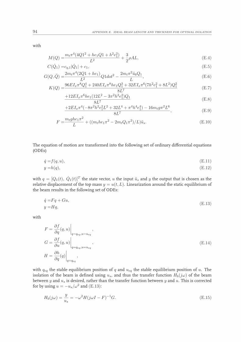
94 APPENDIX E. IDEAL BEAM LENGTH AND THICKNESS FOR OPTIMAL ISOLATION
with
M(Q) =mtπ
4(4Q12 + he1Q1 + h2e21)
L2+
3
2ρAL, (E.4)
C(Q1) =cq,1|Q1|+ c1, (E.5)
G(Q, Q) =2mtπ
4(2Q1 + he1)
L2Q1dot2 − 2mtπ
2ubQ1
L, (E.6)
K(Q) =96EIxπ8Q4
1 + 240EIxπ8he1Q31 + 32EIxπ6(7h2e2
1 + 8L2)Q21
8L7(E.7)
+12EIxπ6he1(12L2 − 3π2h2e21)Q1
8L7(E.8)
+2EIxπ4(−8π2h2e21L
2 + 32L4 + π4h4e41)− 16mtgπ2L6
8L7, (E.9)
F =mtghe1π
2
L+ ((mthe1π
2 − 2mtQ1π2)/L)us. (E.10)
The equation of motion are transformed into the following set of ordinary differential equations(ODEs)
q =f(q, u), (E.11)
y =h(q), (E.12)
with q = [Q1(t), Q1(t)]T the state vector, u the input us and y the output that is chosen as the
relative displacement of the top mass y = u(t, L). Linearization around the static equilibrium ofthe beam results in the following set of ODEs:
q =Fq + Gu,
y =Hq,(E.13)
with
F =∂f
∂q(q, u)
∣
∣
∣
∣
q=qeq ,u=ueq
,
G =∂f
∂u(q, u)
∣
∣
∣
∣
q=qeq ,u=ueq
,
H =∂h
∂q(q)
∣
∣
∣
∣
q=qeq
,
(E.14)
with qeq the stable equilibrium position of q and ueq the stable equilibrium position of u. Theisolation of the beam is defined using us, and thus the transfer function Hb(jω) of the beambetween y and us is desired, rather than the transfer function between y and u. This is correctedfor by using u = −us/ω2 and (E.13):
Hb(jω) =y
us= −ω2H(jωI − F )−1G. (E.15)
95
As only the equations of motion of the beam are taken into account, F is a 2x2 matrix with asfirst row F (1, :) = [0 1], and the vectors G and H are
G =
[
0,mthe1π
2 + 2mtQ1π2
L
]T
, (E.16)
and
H =
[−he1π2 − 2Q1π
2
L, 0
]
. (E.17)
Having (E.15) and the vectors G and H , the isolation of the beam can be written out. First,(jωI − F )−1 is calculated using the exact solution of the inverse of a 2x2 matrix
A−1 =
[
−a22/(−a11a22 + a12a21) a12/(−a11a22 + a12a21)a21/(−a11a22 + a12a21) −a11/(−a11a22 + a12a21)
]
, (E.18)
with a11 element (1,1) of the matrix A, etc. Now, (jωI − F ) is substituted for A and
a11 = jω, (E.19)
a12 = −1, (E.20)
a21 = −F (2, 1), (E.21)
a22 = jω − F (2, 2). (E.22)
As the first element of the vector G and the last element in vector H are zero, only the firstelement in the last column of (jωI−F )−1 is of interest in E.15. Substitution of (E.19) in element(1,2) of (E.18) results in
A−1(1, 2) =−1
−jω(jω − F (2, 2)) + F (2, 1). (E.23)
Substitution of this into (E.15) results in the following transfer function of the beam:
Hb(jω) =ω2H(1)G(2)
−jω(jω − F (2, 2)) + F (2, 1). (E.24)
The isolation of the beam is equal to the magnitude of Hb(jω) at a certain frequency ω, and since|Hb(jω)| =
√
Re(Hb(jω))2 + Im(Hb(jω))2 with,
Re(Hb(jω)) = −ω2−H(1)G(2)ω2 −H(1)G(2)F (2, 1)
(ω2 + F (2, 1))2 + ω2F (2, 2)2, (E.25)
and
Im(Hb(jω)) = −ω2 ωH(1)G(2)F (2, 2)
(ω2 + F (2, 1))2 + ω2F (2, 2)2, (E.26)
the isolation of the beam is
∣
∣
∣
y
u
∣
∣
∣=
−ω2H(1)G(2)√
(ω2 + F (2, 1))2 + ω2F (2, 2)2. (E.27)

96 APPENDIX E. IDEAL BEAM LENGTH AND THICKNESS FOR OPTIMAL ISOLATION
Having the exact expression for the isolation of the beam, the optimization toolbox in Matlab canbe used to find the optimal combination of for instance the beam length L and beam thicknessh to isolate a certain top mass mt from a vibration with frequency f = ω/2/π. One way of doingthis is by using fminsearch(@(X) ISOL(X),[L0 h0]) with ISOL(X) a function file containingE.27, L0 an initial guess for L and h0 an initial guess for h. As the minimum of the functionISOL(X) is sought, the absolute value of one minus the isolation of the beam is used, instead ofthe exact formulation of the isolation.

Appendix F
Influence of order of Taylor series
approximation and number of DOFs
In the validation of the semi-analytical model in Chapter 5, when 1 mode to model the beam wastaken into account, the Taylor series approximation used to approximate the curvature of the beam(3.14) and the inextensibility constraint (3.12)were of order 13, and thus very accurate. Includinghigher modes with this order of Taylor series approximation results in computation problems inMAPLE, the package used to derive the equations of motions. Thus, when 3 modes were usedto model the beam, the order of Taylor series approximation was 3, which is the maximum orderof Taylor series approximation that can be used in a semi-analytical model with N = 3. Themaximum order of Taylor series in the semi-analytical model with N = 2 is 7. This can resultin quite inaccurate results, especially for high values of the relative top mass, which is shown inthis appendix. In all analyses, the imperfection parameters of the second and third beam modeare equal to 0.01, and the damping parameters for these beam modes are set to 0.1. In this way,the (sub)harmonic contributions of the higher modes are limited, and a fair comparison to themodel with only one beam mode can be made.
In Figure F.1, for L = 0.183 [m], e1 = 1.4 [-], E0 = 0.01 [V], and mt = 0.762 [kg] (r0 = 0.214) theSA-model with N = 1 is shown for three order of Taylor series approximation, namely a 3rd, 7th,and 13th order, shown in black, dark gray and light gray respectively. It follows that the three linesmatch, and for this simulation it does not matter which order of Taylor series approximation istaken.
In Figure F.2, for the same experiment, the results of the semi-analytical model with N = 1 andN = 3, using a 3rd order Taylor series approximation, are shown by the black and light gray lines.Clearly, the model with N = 3 differs from the model with N = 1.
In Figure F.3, the results of the semi-analytical model using a 3rd and 13th order for N = 1, a 3rd
and 7th order for N = 2, and a 3rd order for N = 3 for a beam with L = 0.183 [m], e1 = 1.4[-], E0 = 0.01 [V], and mt = 3.224 [kg] (r0 = 0.932) are shown. It follows that the results forN = 1 with 3rd order is similar to N = 2 with 3rd order, which holds also for N = 1 with 13th
order and N = 2 with 7th order. The higher orders differ from the results with the lower orderfor the Taylor series approximation. The results with N = 3 differ from all results with N = 1and N = 2, and can therefore not be trusted.
97

98 APPENDIX F. INFLUENCE OF ORDER OF TAYLOR SERIES APPROXIMATION AND NUMBER OF DOFS
0 20 40 60 80 100 120 140 160 180 20010
−3
10−2
10−1
f [Hz]
U[m
/s]
3rd order7rd order13rd order
Figure F.1: Comparing a 3rd, 7th, and 13th order Taylor series approximation for N = 1,L = 0.183 [m], e1 = 1.4 [-], E0 = 0.01 [V], and mt = 0.762 [kg].
0 20 40 60 80 100 120 140 160 180 20010
−3
10−2
10−1
f [Hz]
U[m
/s]
N = 1, 13rd order
N = 3, 3rd order
Figure F.2: Comparing N = 1 and N = 3 for L = 0.183 [m], e1 = 1.4 [-], E0 = 0.01 [V], andmt = 0.762 [kg].
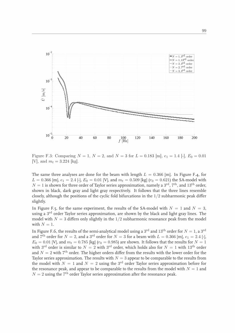
99
0 20 40 60 80 100 120 140 160 180 20010
−5
10−4
10−3
10−2
f [Hz]
U[m
/s]
N = 1, 3rd order
N = 1, 13rd order
N = 2, 3rd order
N = 2, 7rd order
N = 3, 3rd order
Figure F.3: Comparing N = 1, N = 2, and N = 3 for L = 0.183 [m], e1 = 1.4 [-], E0 = 0.01[V], and mt = 3.224 [kg].
The same three analyses are done for the beam with length L = 0.366 [m]. In Figure F.4, forL = 0.366 [m], e1 = 2.4 [-], E0 = 0.01 [V], and mt = 0.509 [kg] (r0 = 0.621) the SA-model withN = 1 is shown for three order of Taylor series approximation, namely a 3rd, 7th, and 13th order,shown in black, dark gray and light gray respectively. It follows that the three lines resembleclosely, although the positions of the cyclic fold bifurcations in the 1/2 subharmonic peak differslightly.
In Figure F.5, for the same experiment, the results of the SA-model with N = 1 and N = 3,using a 3rd order Taylor series approximation, are shown by the black and light gray lines. Themodel with N = 3 differs only slightly in the 1/2 subharmonic resonance peak from the modelwith N = 1.
In Figure F.6, the results of the semi-analytical model using a 3rd and 13th order for N = 1, a 3rd
and 7th order for N = 2, and a 3rd order for N = 3 for a beam with L = 0.366 [m], e1 = 2.4 [-],E0 = 0.01 [V], and mt = 0.785 [kg] (r0 = 0.985) are shown. It follows that the results for N = 1with 3rd order is similar to N = 2 with 3rd order, which holds also for N = 1 with 13th orderand N = 2 with 7th order. The higher orders differ from the results with the lower order for theTaylor series approximation. The results with N = 3 appear to be comparable to the results fromthe model with N = 1 and N = 2 using the 3rd order Taylor series approximation before forthe resonance peak, and appear to be comparable to the results from the model with N = 1 andN = 2 using the 7th order Taylor series approximation after the resonance peak.

100 APPENDIX F. INFLUENCE OF ORDER OF TAYLOR SERIES APPROXIMATION AND NUMBER OF DOFS
0 20 40 60 80 100 120 140 160 180 20010
−5
10−4
10−3
10−2
10−1
100
f [Hz]
U[m
/s]
3rd order7rd order13rd order
Figure F.4: Comparing a 3rd, 7th, and 13th order Taylor series approximation for N = 1,L = 0.366 [m], e1 = 2.4 [-], E0 = 0.01 [V], and mt = 0.509 [kg].
0 20 40 60 80 100 120 140 160 180 20010
−5
10−4
10−3
10−2
10−1
100
f [Hz]
U[m
/s]
N = 1, 13rd order
N = 3, 3rd order
Figure F.5: Comparing N = 1 and N = 3 for L = 0.366 [m], e1 = 2.4 [-], E0 = 0.01 [V], andmt = 0.509 [kg].

101
0 20 40 60 80 100 120 140 160 180 20010
−6
10−5
10−4
10−3
10−2
10−1
f [Hz]
U[m
/s]
N = 1, 3rd order
N = 1, 13rd order
N = 2, 3rd order
N = 2, 7rd order
N = 3, 3rd order
Figure F.6: Comparing N = 1, N = 2, and N = 3 for L = 0.366 [m], e1 = 2.4 [-], E0 = 0.01[V], and mt = 0.785 [kg].

102 APPENDIX F. INFLUENCE OF ORDER OF TAYLOR SERIES APPROXIMATION AND NUMBER OF DOFS

Appendix G
Time signals of lasers during
experiment
On the next four pages, the time signals of the two lasers are shown for two experiments. Fig-ure G.1 shows the time signal of the laser used to measure the velocity of the top mass duringthe first experiment (L = 0.183 [m], mt = 0.762 [kg], E0 = 001 [V]. The signal is shown betweent = 42 and t = 42.2 [s]; the frequency of the harmonic excitation is f = 152 [Hz] during this timeperiod. Figure G.2 shows the time signal of the laser used to measure the velocity of the shakertable during this experiment. The signal of the shaker velocity is less regular than the signalof the top mass velocity: some peaks shown two or more smaller peaks. Figure G.3 shows thetime signal of the laser used to measure the velocity of the top mass during the experiment withL = 0.183 [m], mt = 3.224 [kg], and E0 = 001 [V]. Again, the signal is shown between t = 42 andt = 42.2 [s], and the frequency of the harmonic excitation is again f = 152 [Hz] during this timeperiod. The minimum voltage from the laser is about 0.03 [V], and as the minimum resolutionis used for this laser, which is 110−3 [m/s/V], the velocity measured in this experiments is aboutthe smallest that can be measured. Figure G.4 shows the time signal of the laser used to measurethe velocity of the shaker table during this experiment. Again, the signal of the shaker velocityis less regular than the signal of the top mass velocity: some peaks shown two or more smallerpeaks. It must be noted that the signals of the lasers are shown in voltage, instead of [m/s] as inthe other analyses.
103

104 APPENDIX G. TIME SIGNALS OF LASERS DURING EXPERIMENT
42 42.02 42.04 42.06 42.08 42.1 42.12 42.14 42.16 42.18 42.2−0.1
−0.08
−0.06
−0.04
−0.02
0
0.02
0.04
0.06
0.08
0.1
Time [s]
u(t
,L)
[V]
Figure G.1: Laser signal of top mass for mt = 0.762 [kg] and E0 = 0.01 [V], f = 152 [Hz].

105
42 42.02 42.04 42.06 42.08 42.1 42.12 42.14 42.16 42.18 42.2−0.2
−0.15
−0.1
−0.05
0
0.05
0.1
0.15
0.2
Time [s]
ub(t
)[V
]
Figure G.2: Laser signal of shaker table for mt = 0.762 [kg] and E0 = 0.01 [V], f = 152 [Hz].

106 APPENDIX G. TIME SIGNALS OF LASERS DURING EXPERIMENT
42 42.02 42.04 42.06 42.08 42.1 42.12 42.14 42.16 42.18 42.2−0.08
−0.06
−0.04
−0.02
0
0.02
0.04
0.06
0.08
Time [s]
u(t
,L)
[V]
Figure G.3: Laser signal of top mass for mt = 3.224 [kg] and E0 = 0.01 [V], f = 152 [Hz].

107
42 42.02 42.04 42.06 42.08 42.1 42.12 42.14 42.16 42.18 42.2
−0.25
−0.2
−0.15
−0.1
−0.05
0
0.05
0.1
0.15
0.2
0.25
Time [s]
ub(t
)[V
]
Figure G.4: Laser signal of shaker table for mt = 3.224 [kg] and E0 = 0.01 [V], f = 152 [Hz].