AD-A272 279AEROSPACE REPORT NO.TR-92(2940)-3

On the Theory of Morphology-Dependent Resonances:Shape Resonances, Width Formulas, and Graphical

Representations

Prepared by

B. R. JOHNSONSpace and Environment Technology Center

Technology Operations

DTIC26 October 1993 ELECTE

Prepared for

SPACE AND MISSILE SYSTEMS CENTER .........AIR FORCE MATERIEL COMMAND

2430 E. El Segundo BoulevardLos Angeles Air Force Base, CA 90245

Engineering and Technology Group

THE AEROSPACE CORPORATION

El Segundo, California

APPROVED FOR PUBLIC RELEASE:

93-26,561 DISTRIBUTION UNLIMITED

/ llll /Iil/i/l ll/ l/I/ /// ll/ /IC/i

This report was submitted by The Aerospace Corporation, El Segundo, CA 90245-4691, underContract No. F04701-93-C-0094 with the Space and Missile Systems Center, 2430 E. El SegundoBlvd., Los Angeles Air Force Base, CA 90245. It was reviewed and approved for The AerospaceCorporation by A. B. Christensen, Principal Director, Space and Environment TechnologyCenter. Capt. Francis K. Chun was the project officer for the Mission-Oriented Investigation andExperimentation (MOIE) program.

This report has been reviewed by the Public Affairs Office (PAS) and is releasable to the NationalTechnical Information Service (NTIS). At NTIS, it will be available to the general public,including foreign nationals.

This technical report has been reviewed and is approved for publication. Publication of thisreport does not constitute Air Force approval of the report's findings or conclusions. It ispublished only for the exchange and stimulation of ideas.

WM KYLE SNEDDON, Capt, USAFDeputy Chief, Industrial & Int'l Divis /<v<

FRANCIS K. CHUN, Capt, USAFDeputy Chief, Brilliant Eyes Test & Mission Ops Branch

UNCLASSIFIEDSECURITY CLASSIFICATION OF THIS PAGE

REPORT DOCUMENTATION PAGEla. REPORT SECURITY CLASSIFICATION lb. RESTRICTIVE MARKINGS

Unclassified2a. SECURITY CLASSIFICATION AUTHORITY 3. DISTRIBUTION/AVAILABILIrY OF REPORT

2b. DECLASSIFICATIONiDOWNGRADING SCHEDULE Approved for public release; distribution unlimited

4. PERFORMING ORGANIZATION REPORT NUMBER(S) 5. MONITORING ORGANIZATION REPORT NUMBER(S)

TR-92(2940)-3 SMC-TR-93-54

6a. NAME OF PERFORMING ORGANIZATION 6b. OFFICE SYMBOL 7a. NAME OF MONITORING ORGANIZATIONThe Aerospace Corporation Space and Missile Systems CenterTechnology Operations S

6c. ADDRESS (City, State, and ZIP Code) 7b. ADDRESS (City, State, and ZIP Code)

El Segundo, CA 90245-4691 Los Angeles Air Force BaseLos Angeles, CA 90009-2960

8a. NAME OF FUNDINGSPONSORING 8b. OFFICE SYMBOL 9. PROCUREMENT INSTRUMENT IDENTIFICATION NUMBERORGANIZATION (Nf applicable)________________________jF04701-88-C-0089

Sc. ADDRESS (City, Slate, and ZIP Code) 10. SOURCE OF FUNDING NUMBERS

PROGRAM PROJECT TASK WORK UNITELEMENT NO. NO. NO. ACCESSION NO.

11. TITLE (Include Security Ctassllacation)

On the theory of morphology-dependent resonances: Shape resonances, width formulasand graphical representations

12. PERSONAL AUTHOR(S)

Johnson, B. Robert13a. TYPE OF REPORT 13b. TIME COVER;71D 14. DATE OF REPORT (Year, Month, Day) 15. PAGE COUNT

FROM TO _ _ 1993 October 26 4216. SUPPLEMENTARY NOTATION

17. COSATI CODES 18. SUBJECT TERMS (Continue on reverse If necessary and identify by block numnber)

FIELD GROUP SUB-GROUPMorphology-dependent resonance, Shape resonance, Mie scattering

19. ABSTRACT (ConUnue on reverse i9 necessary and idantfy by block number)

The theory of morphology-dependent resonances of a spherical particle is developed in analogy with the theoryof quantum mechanical shape resonances. Exact analytic formulas for predicting the widths of the resonancesare developed. A useful graphical procedure for organizing and displaying data for a spectrum of resonances isdemonstrated.

20. DISTRIBUTION/AVAILABILITY OF ABSTRACT 21. ABSTRACT SECURITY CLASSIFICATION

E UNCLASSIFIDAJUNLIMrTED ED SAME AS RPT. oTIC USERS Unclassified22a. NAME OF RESPONSIBLE INDIVIDUAL 22b. TELEPHONE (Include Area Code) 22c. OFFICE SYMBOL

DO FORM 1473,84 MAR 83 APR editon may be used nill exKhausted. SECURITY CLASSIFICATION OF THIS PAGEAll other eddios ar obsolete. UNCLASSIFIED

PREFACE

This report presents the results of work sponsorea by the USAF Space and Missile Systems Centerunder Contract No. F04701-88-C-0089.

Aoeession ForNVIS WA&IDTIO TAB 0VnamottoodJustitloatlon

ByDistri bution/

Availability OodoeAIA~ and/or

Diet Speclal

CONTENTS

1. IN T R O D U C T IO N ................................................................................................................. 7

2. SCA'1fERING THEORY ................................................................................................ 9

3. RESO N AN CE THEO RY ..................................................................................................... 15

3.1 QUANTUM MECHANICAL ANALOGY .............................................................. 15

3.2 MDRS INTERPRETED AS SHAPE RESONANCES ............................................. 17

3.3 PARTICLES WITH NEGATIVE DIELECTRIC FUNCTIONS .............................. 23

4. RESON AN CE W IDTH S ...................................................................................................... 27

4.1 TE RESONANCE, REAL INDEX OF REFRACTION ........................................... 27

4.2 TM RESONANCE, REAL INDEX OF REFRACTION ........................................... 29

4.3 TE RESONANCE, COMPLEX INDEX OF REFRACTION .................................... 29

4.4 TM RESONANCE, COMPLEX INDEX OF REFRACTION ..................................... 32

5. GRAPHICAL REPRESENTATION OF THE RESONANCE SPECTRUM ......................... 35

6. SUMMARY AND CONCLUDING REMARKS ................................................................ 39

R E FE R E N C E S ......................................................................................................................... 4 1

3

FIGURES

1. Effective potential associated with a spherical dielectric particle ...................................... 17

2. Graphical Solution to Eqs. (26a,b) ................................................................................ 20

3. Radial wave functions for thc three TE, n = 40 resonances........................................... 21

4. Behavior of the TE wave function in the vicinity of a resonance .................................... 22

5. Effective potential function for a layered sphere with a positive dielectriccore covered by a negative dielectric layer .................................................................... 23

6. Effective potential associated with a negative dielectric particle .................................... 24

7. Graphical representation of TE resonance parameters for a sphericalparticle with index of refraction m = 1.47 .................................................................. 35

8. Width contours for TE resonances of a particle with a complex indexof refraction m = 1.47 + i 0.000001 ............................................................................. 37

9. Height contours for the TE resonances of a particle with complexindex of refraction m = 1.47 + i 0.000001 ................................................................. 38

5

1. INTRODUCTION

The cross section for scattering electromagnetic energy by a dielectric sphere exhibits a series ofsharp peaks as a function of the size parameter. These peaks are a manifestation of scatteringresonances in which electromagnetic energy is temporarily trapped inside the particle. A physicalinterpretation is that the electromagnetic wave is trapped by almost total internal reflection as itpropagates around the inside surface of the sphere, and after circumnavigating the sphere, thewave returns to its starting point in phase. These resonances are now generally referred to asmorphology-dependent resonances (MDRs). A large body of literature has been written on thesubject. A good review article, containing many references to the original literature, has recentlybeen written by Hill and Benner.1

MDRs are responsible for the ripple structure observed in Mie scattering 2 and for the large opti-cal feedback necessary for lasing,3,4 stimulated Raman scattering,5 sum-frequency generation, 6

and other nonlinear processes that have been observed in small droplets. Stimulated Raman scat-tering from small spheres has been proposed as a method for analyzing the chemical concentra-tion and size of droplets in fuel sprays, 7 and the elastic scattering of light near an MDR has beenused to detcrmine chemical composition of aerosol particles.8 MDRs are also responsible forenhanced energy transfer that has been observed in aerosol particles. 9 Laboratory demonstra-tions have recently shown that the MDRs of an ensemble of microspheres can be utilized to con-struct a new type of optical memory. 10

The present paper covers three topics in the theory of MDRs. These are (i) an interpretation ofMDRs as "shape resonances;" (ii) the derivation of exact analytic formulas for predicting thewidths of resonances; and (iii) the demonstration of a useful graphical procedure for displayingresonance data. The theory of shape resonances is a familiar topic in atomic and molecularscattering theory; however, the fact that MDRs can be regarded as shape resonances does notseem to be widely appreciated. In this interpretation, the electromagnetic energy is temporarilytrapped near the surface of the sphere in a "dielectric potential well." The energy enters and exitsthe well by tunneling through a centrifugal barrier. Recently this problem has been studied usingcomplex angular momentum theory. 11,12

This report is organized as follows. Section 2 begins with a review of some of the basic equationsfor electromagnetic scattering from spherically symmetric particles. This section is presentedmainly as a matter of convenience. It helps to establish our conventions and notation and alsogathers together equations that will be needed later. Section 3 discusses resonance theory andshows how MDRs can be interpreted as shape resonances. Also included in this section is arelated discussion of electromagnetic bound states in negative dielectric particles. In Section 4,several new exact analytic formulas for predicting the widths of resonances are developed.Formulas are derived for both real and complex indices of refraction. In Section 5, a usefulgraphical procedure for organizing and displaying the data for a spectrum of resonances is pre-sented. Section 6 includes a summary and concluding remarks.

7

2. SCATTERING THEORY

This section briefly reviews the theory of electromagnetic scattering from a spherical particle.The basic equations needed in the remainder of the report are presented, and some of theconventions and the notation to be used are established. The particle is assumed to benonmagnetic. The radius of the particle is denoted by a and the complex index of refraction,which may be a function of the radial coordinate r, is denoted by m(r) = mr(r) + imi(r). In theregion outside the sphere, r > a, the index of refraction is m(r) = 1, and the wave number is k =

2nIX. The complex time dependence of the electric field is exp(-iwt). This time-dependenceconvention is the same as that used by Bohren and Huffman, 13 but is opposite of that used byVan de Hulst14 and Kerker 15 . With this convention, a positive imaginary part of the index ofrefraction results in power absorption by the particle.

The electric field must satisfy the scattering boundary conditions and the following vector waveequation

VxVXE-k 2m 2(r)E=0. (1)

The solution to this equation is most easily computed by expanding the electric field in terms ofthe spherical vector wave functions,

exp(imo) Sp (r)Xm(0)M"'m(r'O'4O) = kr r)nmekr

N,(r,0,)= exp(im) 1 dT(r) I (r)Z.. (1)]' J k 2m 2(r) Lr 8r + r2 (2)

where the functions Mn,m(r,0,0) are the transverse electric (TE) modes, and the functionsNn,m(r,0,0) are the transverse magnetic (TM) modes. The angular functions in these expressionsare defined as

9

X, (0) = Wi - r.,m (O)i,

17,.m(0) = *r',•(6)e9 -i;,.,,(6)•,

Z...() =n(n + 1)•'(cos e)i, (3)

where

m

;m(0) = P.'(cos 0)sin 0

Tr.,(2) = P(Cos 0). (4)

The function P,"'(cos 0) is the associated Legendre polynomial, and ,, •,,•, are the unitorthogonal vectors associated with spherical coordinates. The functions S.(r) and T (r) are theradial Debye potentials, which satisfy the following second order differential equations 16 ,17

dS(r) + k2m2(r) -n(n + 1 S.(r)=0 5a)

dr2 r r2

_____ _______ F 2 n(n +l)]

d2T,(r) 2 din(r) dT,(r) -k ( T,(r)2=O (5b)dr2 m(r) dr dr r 27 ,(r)

The solutions to these equations must obey the initial conditions S. (0) = 0 and T. (0) = 0. Theseconditions are necessary to ensure that the electric field is finite at the origin.

10

In regions where the index of refraction has the constant value m, the two differential equations(5ab) have the same form, and the linearly independent solutions are Riccati-Bessel functions,18

which are defined as

V. (mkr) = mkrj,(mkr) 6a)

X, (mkr) = mkr n. (mkr) (6b)

where j, (mkr) and n. (mkr) are spherical Bessel functions. In the external region, r > a, wherem(r) = 1, the general solutions are linear combinations of the Riccati-Bessel functions. For lateruse in this report, it will be convenient to define these external solutions as follows:

Sn(r) =B.[Z.(kr)+ P,, V,, (kr)] (7a)

T7(r) = A,[Z.(kr)+ an V,, (kr)] (7b)

where a,],.,A, and B. are constants. These functions must connect, in an appropriate manner,at the surface of the sphere, with the solutions inside the sphere. The connection of the internaland external solutions is most easily carried out using the log derivative formalism.

The "modified log derivative functions" of S.(r) and Tn(r) are defined as

Un (r) = l[S(r) / Sn (r)] (8a)k

V(r) [(r) / (r)], (8b)km'(r)

where the prime denotes the derivative with respect to the argument of the function. Both ofthese functions are continuous at all points. This includes points where the index of refraction is

11

discontinuous, such as at the surface of the sphere or, in the case of a layered sphere, at theboundaries between the layers. It will also be useful to define the log derivatives of the Riccati-Bessel functions by the relations

D. (x) x) (9a)

G,(x) =xW • x,/ W.x (9b)

Substitute the external solutions defined by (7) into the definitions of the modified logarithmicderivatives given by (8) and evaluate at the surface of the sphere. Then use the continuity of thefunctions U,. (r) and V. (r) across the boundary to obtain

U (a)-= X~'(ka) + ,,. •(ka)x.(ka) +/3 / (ka)

_ X(ka) +a,, V. (ka)V (a) = " (ka(10b)X, (ka) + a,, V,, (ka)

where U,,(a) and V,(a) are evaluated from the internal solution. These equations can be solvedfor a,, and P3.. The results are

V,(ka) [DG.(ka)-U,,(a) J

12() D.(ka) - U.(a)

a. = k)G k)-V a (Illb)•(-ka) D,,(ka) - V, (a)

12

For the special case of Mie scattering, in which the index of refraction has a constant value m, the

solutions of the differential equations (5) in the region 0 _ r _ a are given by

S,(r) = T,(r)= IV/(mkr) (12)

Substitute these functions into (8) to obtain

U,(r) = mD• (mkr) (1 3a)

V, (r) =- D, (mkr) (13b)m

These expressions are then substituted into (11) to obtain

= .(x) [G.(x)- mD,,(mx) 1

""x DmG,(x)- D.(mx)

rx) mGZ,, ( x)--- D,-- (- - (14b)

4.(x)in mD.(x) -D(mx) J

where x = ka is the size parameter.

It can be shown that a, and f0, are related to the a. and b, coefficients of Mie theory by theformulas

b,, (15a)1- if'

and

13

a. -(15b)

The aM and b. coefficients defined here are the same as the coefficients defined in Bohren andHuffman13 and are the complex conjugate of the coefficients defined by Van de Hulst 14 and byKerker. 15 All the usual formulas for cross sections and other quantities that are expressed interms of the a. and b, coefficients are applicable.

14

3. RESONANCE THEORY

3.1 QUANTUM MECHANICAL ANALOGYThe second-order differential equations (5) can be recast in a form similar to the radialSchrodinger equation. This well known analogy is useful because one can then formulateproblems in such a way that familiar quantum mechanical techniques can be used. To simplifythe analogy, assume that the Schrtdinger equation is expressed in units such that A2 / 2y = 1(where h is Plank's constant and y is the reduced mass). The radial Schrmdinger equation thenhas the form

______ (n+ 1)1dr2 L-V(r) + V (r + i)/(r) = EVp'(r) , (16)dr2 I r J 2'

where V(r) is the potential energy function and E is the total energy. Equation (5a) will beidentical in form to the Schrwdinger equation if we define the potential to be

V(r) = k2 [1 - m 2 (r)] (17)

and the energy to be

E=k2 (18)

[Equation (18) was obtained by comparing the equations for the case of free space, i.e., form(r) = 1 and V(r) = 0.] We note immediately that one noteworthy difference between thequantum mechanical and electromagnetic cases is that, in the latter case, the potential function isdirectly proportional to the "energy" (i.e., to k2) whereas in the former case V(r) is usually afixed function, independent of the energy. This difference will lead to some interestingconsequences that will be discussed in section 3.3.

The "total potential" is the sum of the potential function, V(r), and the "centrifugal" potential. Itis given by

V.(r) = k2 [1- m2 (r)] n(n+ 1)5 (19)

15

The local wave number, p. (r), is defined by the relation p' (r) = E - V. (r). This can also bewritten in the form

p2(r)=k 2m 2(r) n(n+(20)

The quantity p,2 (r) is analogous to the kinetic energy in quantum mechanics. A region isclassically allowed or classically forbidden depending on whether p,2 (r) is positive or negative,respectively.

Consider the special case of a spherical particle with a constant index of refraction m. Thepotential, in this case, is given by

k2( M2)+n(n+l)/r 2 ra (21)= (21)

V.(r L n(n + 1) / r r > a .

Whether this potential is attractive or repulsive will depend on the values of both m2 and k2 . Thecase of most interest in this report is that of a dielectric particle with M2 > 1 and with k2 >1.(Other cases will be considered in Section 3.3.) As a specific example, consider the potentialfunction V4(r) for a particle of radius a, index of refraction m = 1.47, and wave numberk = 33 / a. For convenience, we choose the unit of length to be equal to the particle radius.Thus, a = 1.0, and k = 33. The potential function, V4 (r), for this case, is shown drawn to scalein Fig. 1. The most striking feature of this function is the presence of a potential well in theregion r, < r < a. This is a classically allowed region in which p,(r) > 0. The well is surroundedby the two classically forbidden regions 0:< r < r, and a < r < r2 in which p2(r) < 0. The pointsrj and r2, defined by the relation p, (r) = 0, are called the classical turning points.

In the equivalent quantum mechanical problem, a particle can tunnel through the classically for-bidden region, a < r < r2, into the classically allowed potential well. For certain values of theenergy, the particles will become temporarily trapped in the well, oscillating back and forth manytimes before finally tunneling back through the classically forbidden region to the outside worldagain. These quasi-bound states are also known as resonances. The type of resonance describedhere is called a shape resonance. The name "shape resonance" means simply that the resonancebehavior arises from the "shape" of the potential, i.e., the well and the barrier. 19 This particulartype of shape resonance, in which the barrier is formed by the centrifugal potential, is also referredto as an orbiting resonance. 20 This latter name is particularly apt considering the usual interpreta-tion of MDRs in terms of light rays propagating around the inside surface of the sphere.'

16

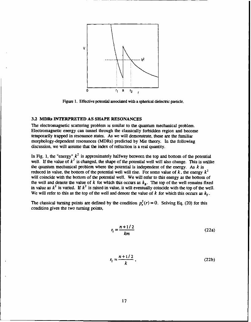
V

0 r, a r2 r

Figure 1. Effective potential associated with a spherical dielectric particle.

3.2 MDRs INTERPRETED AS SHAPE RESONANCESThe electromagnetic scattering problem is similar to the quantum mechanical problem.Electromagnetic energy can tunnel through the classically forbidden region and becometemporarily trapped in resonance states. As we will demonstrate, these are the familiarmorphology-dependent resonances (MDRs) predicted by Mie theory. In the followingdiscussion, we will assume that the index of refraction is a real quantity.

In Fig. 1, the "energy" k2 is approximately halfway between the top and bottom of the potentialwell. If the value of k2 is changed, the shape of the potential well will also change. This is unlikethe quantum mechanical problem where the potential is independent of the energy. As k isreduced in value, the bottom of the potential well will rise. For some value of k, the energy k2

will coincide with the bottom of the potential well. We will refer to this energy as the bottom ofthe well and denote the value of k for which this occurs as k.. The top of the well remains fixedin value as k2 is varied. If k2 is raised in value, it will eventually coincide with the top of the well.We will refer to this as the top of the well and denote the value of k for which this occurs as kT.

The classical turning points are defined by the condition p. (r) = 0. Solving Eq. (20) for thiscondition gives the two turning points,

n+1/2 (22a)/on

n+1/2r2 - k (22b)

k

17

where we have replaced [n(n + 1)112 with n + 1 / 2 and used the fact that m(rj) = m, andm(r2) = 1. These expressions for the turning points can be used to calculate the values of k. andkr. When k = k., the inner turning point must satisfy the relation r, = a, and when k = kr, theouter turning point must satisfy 1.ie relation r2 = a. Substituting these conditions into Eqs. (22)and solving for k gives k. = (n + I / 2) / ma, and kr = (n + I / 2) / a. It is more convenient toexpress these relations in terms of the dimensionless size parameter x = ka rather than k. Thus,the condition for the bottom and top of the potential well is given by

n+1/2XB =n1 (23a)

XT =n+/12. (23b)

In quantum mechanics, only certain discrete energy levels are allowed in a one-dimensionalpotential well. The mathematical reason for this is that the boundary conditions can only besatisfied at these discrete energies. The problem of shape resonances is very similar. Theresonances occur only for energy values that satisfy the boundary conditions, which are quitesimilar to the boundary conditions for the bound-state problem.

The boundary conditions at r = 0 are given by S. (0) = T.(0) = 0. These conditions, which westated previously, must be met by all scattering solutions regardless of whether or not they areresonance states. The solutions that satisfy this condition are given by Eq. (12). The generalform of the solutions in the region r > a is given by Eq. (7). These functions are a linearcombination of the Riccati-Bessel functions 41,,(kr) and Z,(kr). In the classically forbiddenregion, a < r < r2 , these two functions have opposite behavior. The function Vu,(kr) exhibits avery rapid, "exponential-like" growth in this region while the function ZX (kr) exhibits an"exponential-like" decrease. At r = r2 , these functions cease their exponential-like behavior andbegin an oscillatory behavior in the region r2 < r < -.

The condih.on that determines the discrete energy levels of a quasibound shape resonance is therequirement that the wave function exhibit an exponential-like decay in the barrier region so thatif the barrier extended to r -- c, the wave function would decay to zero, and the quasiboundstate would become a true bound state. This means that only the (exponential-like) decreasingfunction X, (kr) is allowed in the barrier region. Translating this requirement back to the wavefunctions defined by Eq. (7) implies that the coefficient that multiplies the (exponential-like)increasing function V, (kr) must be zero, i.e., 1P, = 0 (a,, = 0) at the location of a TE (TM)resonance, respectively. These conditions, which were obtained by satisfying the conditions for ashape resonance, are equivalent to the conditions commonly used to define the location of amorphology-dependent resonance.1 This is evident from Eqs. (15a,b), which show that fin = 0(a., = 0) is equivalent to the condition that the imaginary part of the Mie coefficient b. (a.) beequal to zero.

18

Substituting .6. = 0 and a, = 0 into the Eqs. (14) give the following equations that must besatisfied at the locations of TE and TM resonances, respectively:

G.(xo) =rD.(mxo) (24a)

mG,(x,) = D.(mx=) (24b)

A graphical illustration of these equations is quite illuminating. For this illustration, it issomewhat more convenient to work with the following functions;

d,(mx) = D.'(mx) 25a)

g(TE)(X) = mG.-1 (x) (25b)

S= 1(25c)m

The conditions, given by Eqs. (24), for the TE and TM resonances are now expressed as

g(TE)(x) = d,, (mx) (26a)

g(') (x) = dr(mx). (26b)

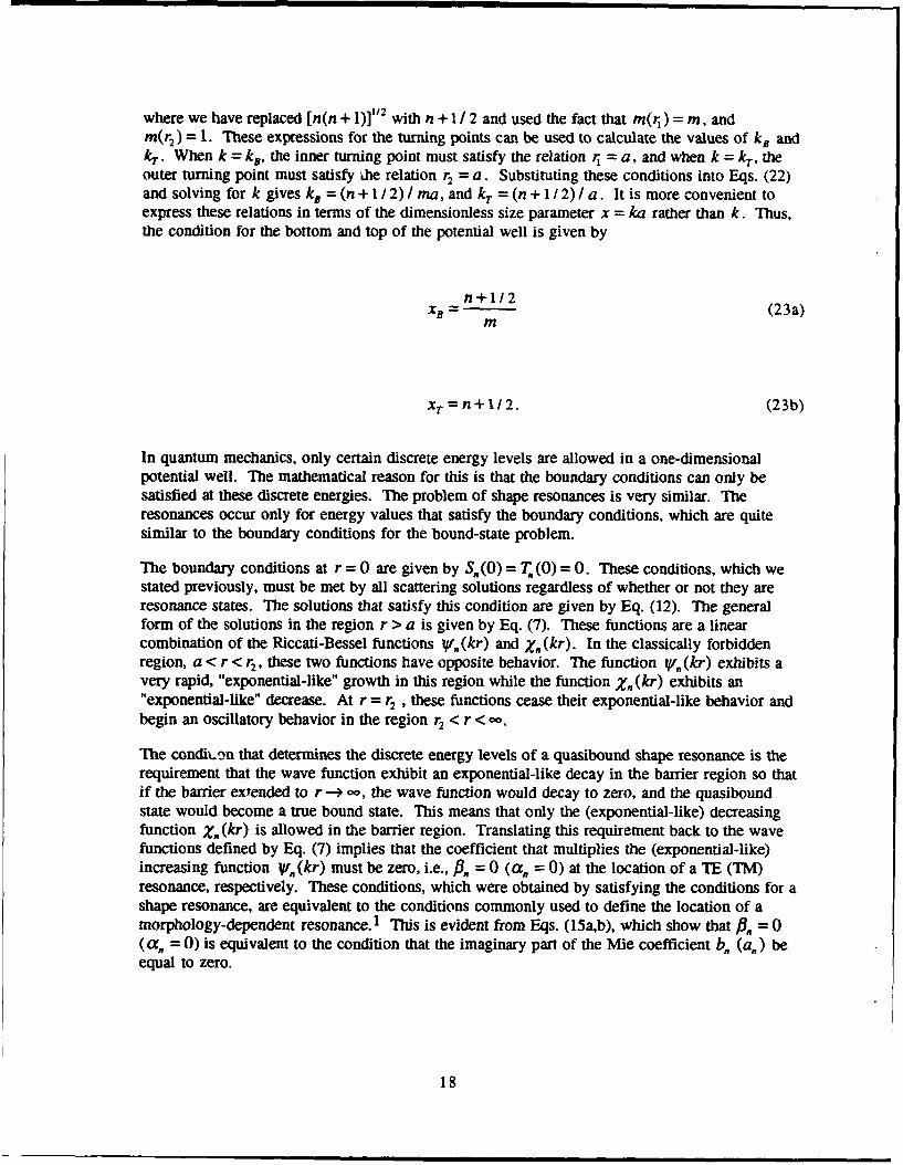
These functions are shown graphically in Fig. 2 for the case m = 1.47 and n = 40. Theintersection points of the curves are the graphical solutions to the resonance equations. It isobvious from the graph that the n = 40 potential supports three TE and three TM resonancesbetween the bottom and top of the potential well, XB = 27.5 and xr = 40.5. In addition, one cansee from the graph that the size parameter for a TE resonance is always slightly less thaci for theequivalent TM resonance. An accurate computer solution of these equations gives the following

19

results: the TE resonances are located at 31.058854, 34.611195, and 37.653070 and the TMresonances are located at 31.519210, 34.996041, and 37.908035. The curves shown in Fig. 2continue to intersect at an infinite number of points in the region x > XT, i.e., above the top of thepotential well. In general, the electromagnetic modes at these points are not counted asresonances because they are too wide to have the general properties associated with a resonance,such as a sharp spike in the scattering cross section. These "above the top of the well" states willbe discussed further in Section 5.

10

d

0g (TE) '

-100 10 20 30 40

xFigure 2. Graphical Soluton to Eqs. (26ab). Intersection points are the sizeparameters of the TE and TM resonances in the region between the bottom andtop of the potential well.

20

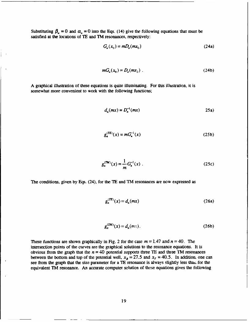
The wave functions for the three TE resonances are shown graphically in Fig. 3. These wavefunctions are the Debye potential functions, So(r), obtained by solving Eq. (5a). They areshown superimposed, at the proper level, on the potential function V4o(r). Within the region ofthe potential well, these wave functions resemble bound states. The lowest level wave function hasa single peak, the next level has two peaks (positive and negative), and the third level has threepeaks. The number of peaks in the classically allowed region of the potential well , r, r •a, iscalled the order number and is denoted by 1. This number, along with the mode number n andthe label TE or TM, uniquely identifies a resonance. Electromagnetic energy is temporarilytrapped in the potential well. It can enter and leave by tunnelling through the outer centrifugalbarrier of the potential well. The width of the resonance is inversely proportional to the lifetimeof the trapped energy, which, in turn, is determined by the rate of tunneling through the barrier.The levels near the bottom of the well must tunnel through a larger barrier than the upper levels.Therefore, the lower levels have a longer lifetime and hence a narrower width than the upperlevels. The widths of the three TE resonances (which were calculated using Eq. (34) in thefollowing section) are 0.00008782, 0.01023, and 0.1297.

x = 37.653070

x =34.611195

X •_= 31.058854

Figure 3. Radial wave functions for the three TE, n = 40 resonances.

21

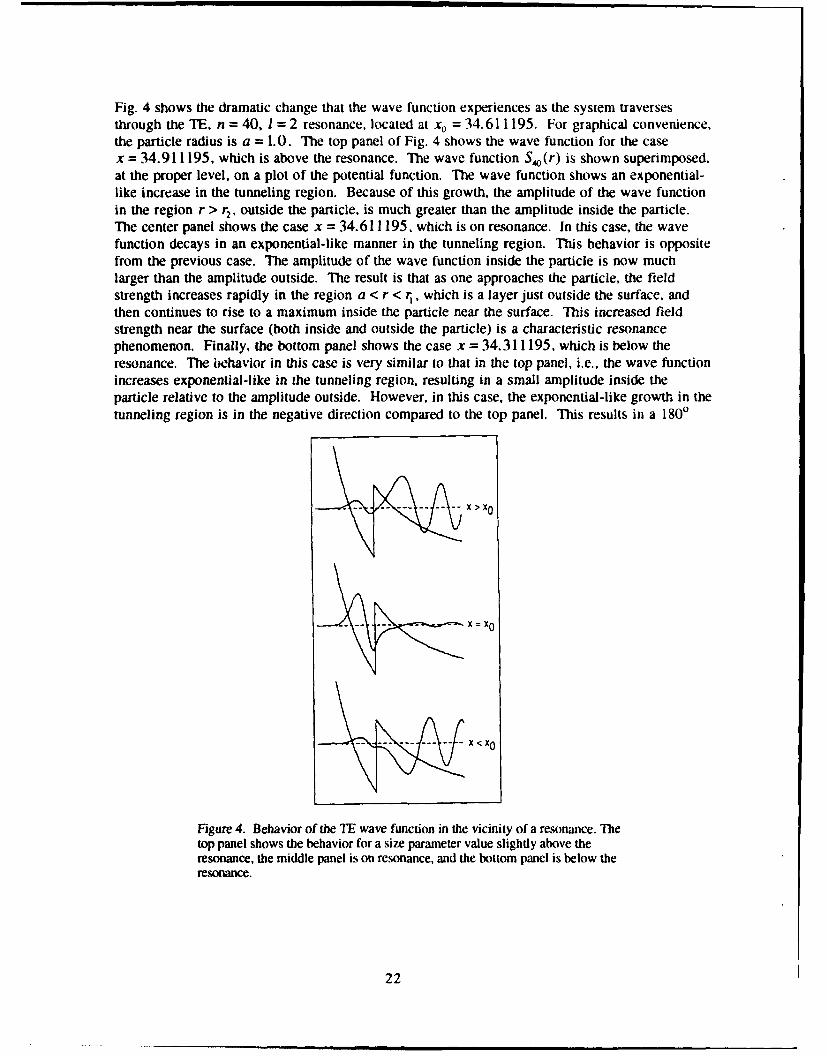
Fig. 4 shows the dramatic change that the wave function experiences as the system traversesthrough the TE, n = 40, 1 = 2 resonance, located at x0 = 34.611195. For graphical convenience,the particle radius is a = 1.0. The top panel of Fig. 4 shows the wave function for the casex = 34.911195, which is above the resonance. The wave function S4o(r) is shown superimposed,at the proper level, on a plot of the potential function. The wave function shows an exponential-like increase in the tunneling region. Because of this growth, the amplitude of the wave functionin the region r > r,, outside the particle, is much greater than the amplitude inside the particle.The center panel shows the case x = 34.611195, which is on resonance. In this case, the wavefunction decays in an exponential-like manner in the tunneling region. This behavior is oppositefrom the previous case. The amplitude of the wave function inside the particle is now muchlarger than the amplitude outside. The result is that as one approaches the particle, the fieldstrength increases rapidly in the region a < r < r,, which is a layer just outside the surface, andthen continues to rise to a maximum inside the particle near the surface. This increased fieldstrength near the surface (both inside and outside the particle) is a characteristic resonancephenomenon. Finally, the bottom panel shows the case x = 34.311195, which is below theresonance. The behavior in this case is very similar to that in the top panel, i.e., the wave functionincreases exponential-like in the tunneling region, resulting in a small amplitude inside theparticle relative to the amplitude outside. However, in this case, the exponential-like growth in thetunneling region is in the negative direction compared to the top panel. This results in a 1800

- - ---- --- x>xO

--------------- x<x0

Figure 4. Behavior of the TE wave function in the vicinity of a resonance. Thetop panel shows the behavior for a size parameter value slighty above theresonance, the middle panel is on resonance, and the bottom panel is below theresonance.

22

phase shift of the outside wave function compared to its phase in the top panel. This 1800 phaseshift is also a characteristic feature of a shape resonance.

The amplitudes of the wave functions shown in Figs. 3 and 4 cannot be directly compared witheach other because each of these fu"tions has been individually normalized to fit on the graph.To compare the peak amplitudes, it is necessary to normalize the wave functions so that they allhave the same amplitude at r -- -c. If we choose the wave amplitude at infinity to be 1. thefollowing results are obtained: The peak amplitudes of the wave functions shown in Fig. 3 are(from top to bottom) 5.00, 18.67, and 225.25. The peak amplitudes (inside the particle) for thewave functions shown in Fig. 4 are (from top to bottom) 0.379, 18.67, and 0.274.

The picture that has been developed in this section, which portrays an MDR as a quasi-boundstate, trapped in a potential well and connected to the outside world by tunneling, gives addedintuition and insight into the nature of electromagnetic scattering resonances. This intuition isespecially valuable for more complicated problems in which the particle has a layered structure2 1

or a continuously varying index of refraction 22.

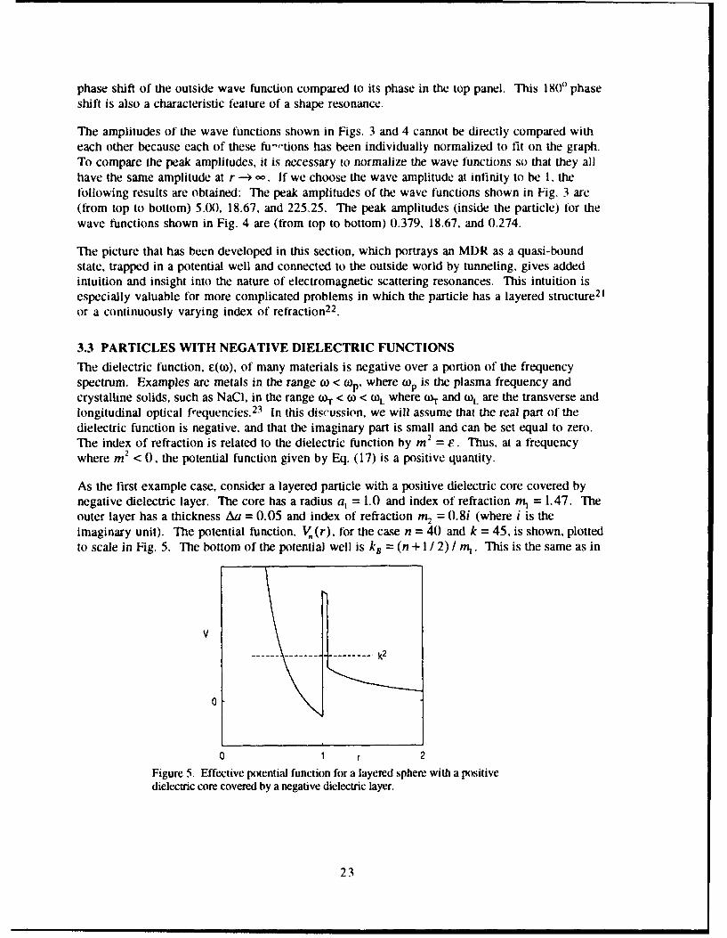
3.3 PARTICLES WITH NEGATIVE DIELECTRIC FUNCTIONSThe dielectric function, £(wo), of many materials is negative over a portion of the frequencyspectrum. Examples are metals in the range w < a)I, where op is the plasma frequency andcrystalline solids, such as NaCI, in the range 0oT < W < WoL where ulr and COL are the transverse andlongitudinal optical frequencies. 23 In this discussion, we will assume that the real part of thedielectric function is negative, and that the imaginary part is small and can be set equal to zero.The index of refraction is related to the dielectric function by m2 = F. Thus, at a frequencywhere m2 < 0, the potential function given by Eq. (17) is a positive quantity.

As the first example case, consider a layered particle with a positive dielectric core covered bynegative dielectric layer. The core has a radius a, = 1.0 and index of refraction in1 = 1.47. Theouter layer has a thickness Aa = 0.05 and index of refraction m2 = 0.8i (where i is theimaginary unit). The potential function, V, (r), for the case n = 40 and k = 45, is shown, plottedto scale in Fig. 5. The bottom of the potential well is k, = (n + 1 / 2) / nh. This is the same as in

V

0

0 1 r 2

Figure 5. Effective potential function for a layered sphere with a positivedielectric core covered by a negative dielectric layer.

23

the previous example problem. However, there is no top to the potential well as definedpreviously. That is, there is no value kT for which k 2 coincides with the top of the well. As thevalue of k2 is increased, the top of the barrier also increases in such a manner that it alwaysexceeds k2. The wave function can tunnel through this barrier and become temporarily trappedin resonant states just as in the previous analysis.

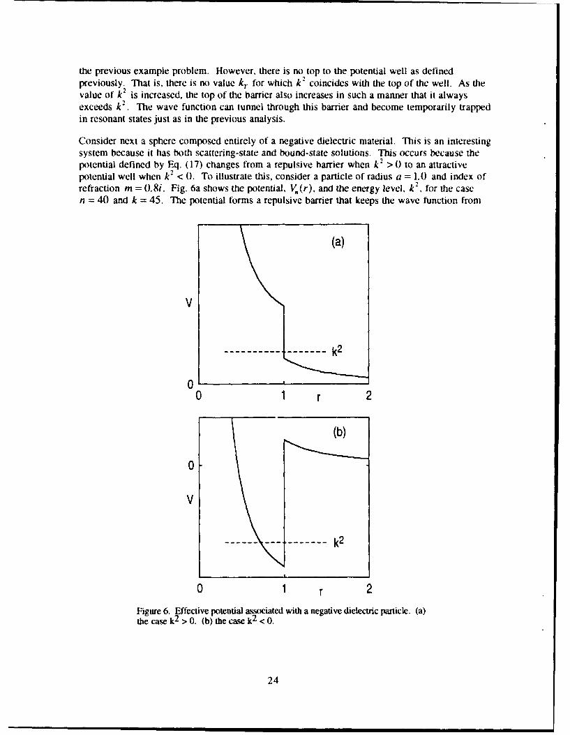
Consider next a sphere composed entirely of a negative dielectric material. This is an interestingsystem because it has both scattering-state and bound-state solutions. This occurs because thepotential defined by Eq. (17) changes from a repulsive barrier when k 2 > 0 to an attractivepotential well when k2 < 0. To illustrate this, consider a particle of radius a = 1.0 and index ofrefraction m = 0.8i. Fig. 6a shows the potential, V.(r), and the energy level, k2, for the casen = 40 and k = 45. The potential forms a repulsive barrier that keeps the wave function from

(a)

V

01 r 2

(b)

0

V

0 1 r 2

Figure 6. Effective potential associated with a negative dielectric particle. (a)the case k2 > 0. (b) the case k2 < 0.

24

penetrating beyond a skin depth into the particle. The region inside the particle is classicallyforbidden and the region outside is classically allowed. This situation is reversed if we let k2 < 0.Then the classically allowed region is inside the particle, and the classically forbidden region isoutside. This is shown in Fig 6b where the system is identical to that in Fig 6a with the exceptionthat we now let k = 70i. Because k2 < 0, the potential is negative. Thus, an attractive potentialwell is formed as shown. This situation is analogous to the quantum mechanical bound-stateproblem. Only selected eigenvalues of k2 are allowed because the wave function must satisfyboundary conditions similar to those for resonances. The difference, in this case, is that the wavefunction cannot tunnel through a barrier, but must continue to decay exponentially to zero.Thus, these are true bound states. There is no radiative energy loss. (However, the inevitableinternal energy loss that occurs in any real system will cause these modes to decay. In order forthese modes to exist, there must be some mechanism to pump energy into them to replace theinternal losses.) A part of the wave function penetrates into the forbidden region outside of thesphere to form an evanescent wave near the surface of the sphere.

The allowed eigenvalues of k can be computed in a manner analogous to that used to calculatethe locations of the resonances. The spectrum of eigenvalues, k2., , forms a sequence of negative

values that begins at the upper (least negative) value and decreases in quantized steps for 1 =1,2,3,.... An upper bound to this sequence is obtained when k 2 coincides with the bottom of thepotential well. This upper bound (which is a negative number) is given by

k 2 n(n + 1)m 2a 2 (27)

For the example case we are considering, k2 = -2562.5 (i.e., ku = 50.62i ). The spectrum ofeigenvalues k.", begins at a value below this upper bound and forms a decreasing sequence ofquantized levels that continues without end. In quantum mechanics, the energy eigenvalues beginat a ground state near the bottom of the potential well and increase in quantized steps. At firstsight, the present system does not seem to behave this way since the eigenvalues decrease inquantized steps. The reason for the apparent difference is because the bottom of the potentialwell is decreasing at an even faster rate than the eigenvalues k2 . Therefore, the interval betweenthe levels k•,t and the bottom of the well actually increase in quantized steps exactly as in thequantum mechanical case.

25

4. RESONANCE WIDTHS

Useful analytic expressions for calculating resonance widths are derived in this section. Theseformulas cover the four cases involving TE and TM resonances for both real and complex indicesof refraction.

4.1 TE RESONANCE, REAL INDEX OF REFRACTION

A "rE resonance is characterized by a sharp peak in the real part of the b, (x) coefficient. 1 Theresonance is located at a size parameter that satisfies the relation (3,(xo) = 0. Since the index ofrefraction is real, it follows from Eq. (14a) that the function fl, (x) is real. This fact, combinedwith Eq. (15a), gives the following expression for the real part of b.(x)

Refb.(x)] = 1 (28)

At the center of the resonance this function has a maximum value Re[b. (xo)] = 1, which dropsoff sharply on either side of x0 . The width of the resonance, w, (xo), is defined to be the distancebetween the points x., on either side of x0 where the amplitude has decreased to half itsmaximum value, i.e., to Re[b.(x,,)] = 1/ 2. It follows from Eq. (28) that the half-amplitudepoints satisfy the relation #.((x:,) = 1.

To a good approximation, the function f8,(x) can be represented by the linear term of a Taylorseries expansion around x0,

AW(x) = fP.3(xo)(x - x0), (29)

where the prime denotes the derivative with respect to x. Within this linear approximation, thehalf amplitude points are x.. = x0 ± Ax, where fl.(xo) )Ax 1. Thus, the width is given by

2w. (xo) = 2 (30)

Differentiate expression (14a) with respect to x and evaluate the result at x0. The result is

27

•(XO) - -() ("a") G'(x0 ) 1 (31)V,,, (xo) mD,, (mX)-D,, (x)

This expression can be simplified with the aid of the following formulas

, (x) = + 1) - D,2,(x), (32a)

n(n + )(x) = (32)

and

G,, (x) - D. (x) = g(x)X,, (x)]-'. (33)

The latter formula was obtained by use of the Wronskian relation for Riccati-Bessel functions.

Substitute the derivatives given by Eq. (32) into Eq. (31). Then use Eq. (24a) to replacemD(mxo) by G(x,). Finally, use Eq. (33) to simplify the result. The result of all thismanipulation is a very simple expression for P(xo), which can be substituted into Eq. (30) togive the following simple analytic formula for the width of a TE resonance:

w"(x°) = (M 2 2 (34)28 1).Z2(XO)

28

4.2 TM RESONANCE, REAL INDEX OF REFRACTION

Using the same analysis as in the previous case, the following expression is obtained for the widthof a TM resonance:

2( =,(x- (35)

Differentiate expression (14b) to obtain

.,'(X)=m"Xo(x) [G.(x0,)-D,,(mx0) 136Vx(x0) LmD.(xO-D,(nx)J(36)

Equations (32), (33) and (24b) are then used to simplify this expression. Substitute thesimplified result into Eq. (35) to obtain the following "exact" formula for the TM resonance

(X0 = 2 (37)(mI - 1)42(Xo) n(--n +:1) + G(xo)]

IM2 X2 I\OLmxo

4.3 TE RESONANCE, COMPLEX INDEX OF REFRACTION

If the index of refraction is allowed to become complex, the function fl,(x), which dependsparametrically on m = mr + imi, will also be complex. To explicitly indicate this dependence, wewill write P3,(m;x). The Taylor series expansion of P3,(m;x), which was carried out previouslywith respect to the size parameter, x, can be extended to also include an expansion with respect tothe index of refraction, m. The size parameter, x,will be expanded around the resonance pointx0, as in our previous analysis, and the index of refraction m will be expanded along theimaginary axis around the point m = mr. The result is

29

f(fl(m;x) = fl.(mXo)(X - XO)+ iy,(m;x). (38)

where the imaginary component, y(m;x), is given by

Y, (M; x) = mi XL --f•,m .x=) (39)

The subscript on the bracket in the above expression indicates that the derivative is to beevaluated at m = mr.

Substitute the linear approximation (38) into Eq. (15a) and calculate the real part of b,,(x). Theresult is

Re[b (x)] (40)R[1+y ] 2+[3;(x-xo)](

This function exhibits a resonance peak centered at x0 . Thus, the position of the resonance is notaltered by adding a small imaginary component to the index of refraction. However, themaximum value of the resonance peak at x. is changed. Evaluating Eq. (40) at xo gives

Re[b1(x0 )] (41)

The width of the resonance is defined to be the distance between the points where the amplitudehas decreased to half of its maximum value. Thus,

1Re[b.(xo ± Ax)] =(42)

2(1+0y.)

30

The maximum amplitude of the resonance peak at xo is called the resonance height 24 and will bedenoted by HR(mi;xo). Combine Eqs. (41) and (43) to obtain the following useful expression

H,(mi;xo)= w.(O;x°) (44)w"(mi;x 0 )

This formula shows that the product of the height and width of the resonance is a constant, equalto the "undamped" width w,(O;xo). The resonance height is a useful quantity because it is ameasure of how much a resonance is suppressed by the internal energy absorption. If no energyis absorbed, the height has a maximum value of 1. If the height is very much less than 1, then theresonance is, for all practical purposes, suppressed out of effective existence.

Differentiate Eq. (14a) with respect to m to get

do - x.(xo) D.(mzO)+mxOD.(mxO)1 (45)dm = g(xo) I mD (mxo)-D.(x0 ) J]

Use Eqs. (32), (33) and (24a) to simplify this expression. The result is

-= XZ2(XO) {[1m- 1]-[G.(xo)+ G.,(xO)/xO]} (46)

dm m

Substitute this into Eq. (39) to get

y'. (M; Xo 0 Z;,2(Xo)(mr )i" 2.Io (47)

where ER is given by

E = [G,(xo)+G,(xo)l x0]. (48)

31

Combine the results contained in expressions (34), (43) and (47) to obtain the following formulafor the width of a TE resonance:

w, (mr;x0) = w,,(0;xo)+ 2xo, m(1C( - E). (49)m,

The quantity E, can be evaluated by an approximate semiclassical WKB analysis. The resultshows that JE, I = 01[] / n where 0[11] is a number of order unity. Therefore, for most resonances1E.1 << 1, and, to a good approximation, it can be neglected in Eq. (49). Thus, the final simplifiedresult for the width of a TE resonance is

W.(r;X0 ) = +2x 0 MI. (50)w(m2 _ 1),X (x0) Mr

The second term in the above expression, which is due to internal energy losses, sets a lower limiton the width of a resonance. This term was derived previously by Arnold using a physicalargument based on a consideration of absorptive energy losses in a cavity.9 It prevents theextremely narrow resonances that are sometimes predicted by theory when mi is neglected. Eqs.(49) and (50) show that the width is a linear function of mi, as has been previously reported. 24' 25

This result can be used in Eq. (44) to calculate the height of the resonance. It is apparent that, incases where the undamped resonance width, w.(O;xo), is extremely small, a small value of mi canlead, for all practical purposes, to the complete suppression of the resonance.

4.4 TM RESONANCE, COMPLEX INDEX OF REFRACTION

The analysis of this case is identical to the previous case with a, and a, replacing fl,, and b,,.Equation (14b) for aI,(m;x) must be differentiated with respect to mr. The result, aftersimplifying with the aid of Eq. (24b), is

da,. = Z.(X0) [xoD (in-o)- G(xo) (51)drm V',,(xo)L G(xo)-D(xo) J

32

This result can be further simplified with the use of Eqs. (33), (32a) and (24b). The result is

d Z.(x0 ) X + M2XO n(n + 1)] (52)0 m [x +mXXoGO(Xo) m52)

Then, with the aid of expressions (37) and (43), we obtain the following formula for the width ofthe TM resonance:

(53)•,,m,;o) •. (0;xo) + 2xom--1- ),(3mr

where

G-.G(xo)- G,,(xo) x 54(M2_1 ) n(n +1)1

LI 0 m 2+XO2

Similar remarks apply to the quantity T, as applied to the quantity E" defined by Eq. (48). Formost res o Enc << 1 and can be neglected. Therefore, the final simplified result for thewidth of a TM resonance is

W.(mi;Xo) = 2 +2xo ML. (55)

33 '2 X2 +G,(Xo)]

33

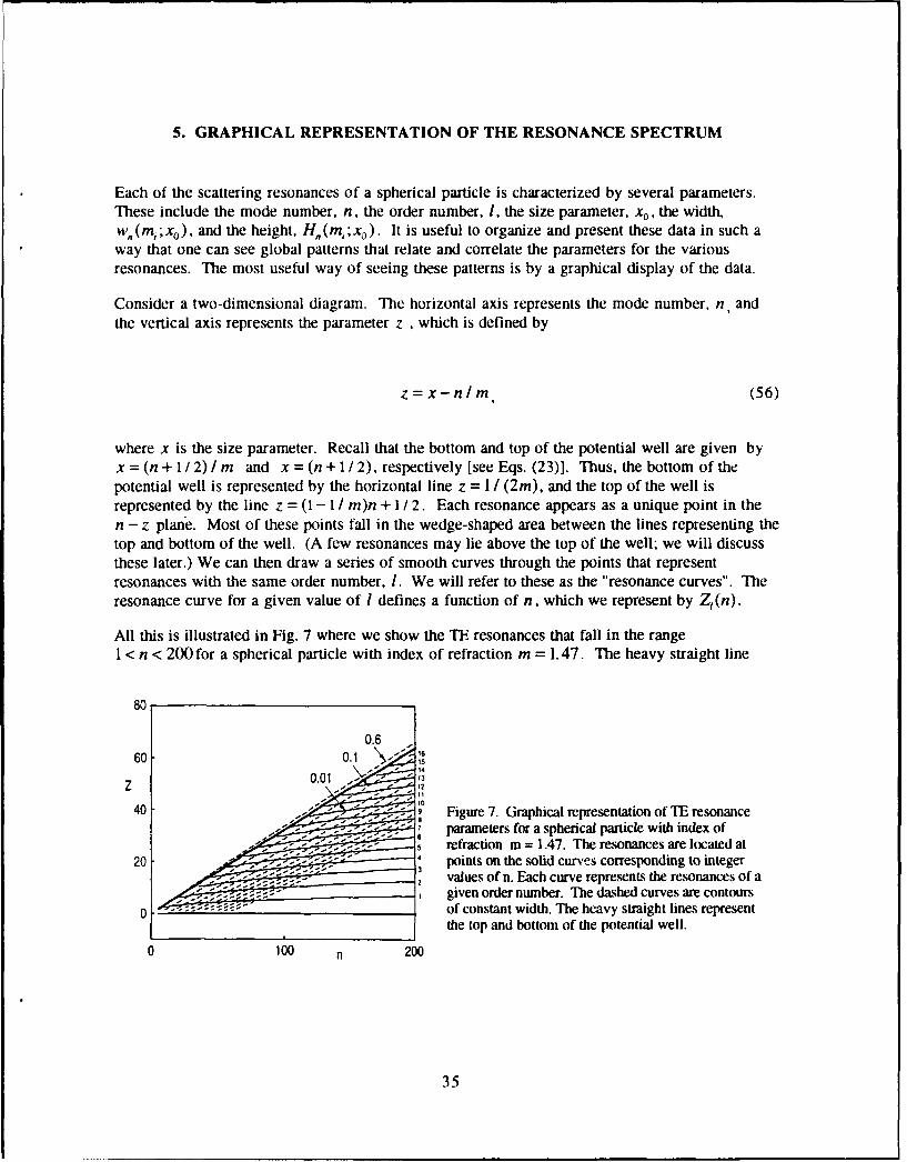
5. GRAPHICAL REPRESENTATION OF THE RESONANCE SPECTRUM

Each of the scattering resonances of a spherical particle is characterized by several parameters.These include the mode number, n, the order number, 1, the size parameter, x0 , the width,w.(m,;x.), and the height, H,(m,;x0 ). It is useful to organize and present these data in such away that one can see global patterns that relate and correlate the parameters for the variousresonances. The most useful way of seeing these patterns is by a graphical display of the data.

Consider a two-dimensional diagram. The horizontal axis represents the mode number, n andthe vertical axis represents the parameter z , which is defined by

z=x-nlm (56)

where x is the size parameter. Recall that the bottom and top of the potential well are given byx = (n + I / 2) / m and x = (n + 1 / 2), respectively [see Eqs. (23)]. Thus, the bottom of thepotential well is represented by the horizontal line z = 1 / (2m), and the top of the well isrepresented by the line z = (1 - I / m)n + 1 / 2. Each resonance appears as a unique point in then - z plane. Most of these points fall in the wedge-shaped area between the lines representing thetop and bottom of the well. (A few resonances may lie above the top of the well; we will discussthese later.) We can then draw a series of smooth curves through the points that representresonances with the same order number, I. We will refer to these as the "resonance curves". Theresonance curve for a given value of I defines a function of n, which we represent by Z, (n).

All this is illustrated in Fig. 7 where we show the TE resonances that fall in the range1 < n < 200 for a spherical particle with index of refraction m = 1.47. The heavy straight line

80

0.6 .60 0.1

Z ;.,,- 10z40 - : - - -

40 - - ;. Figure 7. Graphical representation of TE resonance- -- ,- -- parameters for a spherical particle with index of

"refraction m = 1.47. The resonances are located at20 - -- "- - points on the solid curves corresponding to integer

values of n. Each curve represents the resonances of agiven order number. The dashed curves are contours

0 -of constant width. The heavy straight lines representthe top and bottom of the potential well.

0 100 n 200

35

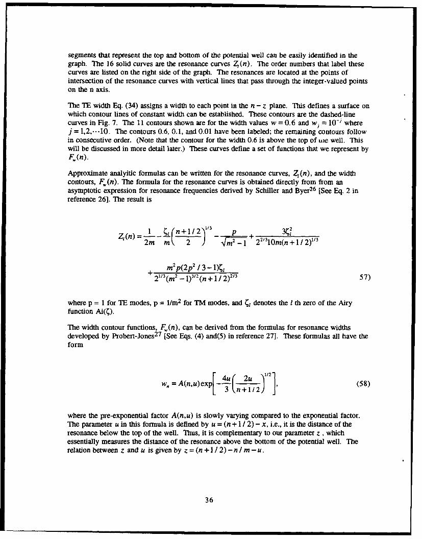
segments that represent the top and bottom of the potential well can be easily identified in thegraph. The 16 solid curves are the resonance curves 4(n). The order numbers that label thesecurves are listed on the right side of the graph. The resonances are located at the points ofintersection of the resonance curves with vertical lines that pass through the integer-valued pointson the n axis.

The TE width Eq. (34) assigns a width to each point in the n - z plane. This defines a surface onwhich contour lines of constant width can be established. These contours are the dashed-linecurves in Fig. 7. The 11 contours shown are for the width values w = 0.6 and wi = 10-l wherej = 1,2,-.-10. The contours 0.6, 0.1, and 0.01 have been labeled; the remaining contours followin consecutive order. (Note that the contour for the width 0.6 is above the top of we well. Thiswill be discussed in more detail later.) These curves define a set of functions that we represent byF~(n).

Approximate analyitic formulas can be written for the resonance curves, Z (n), and the widthcontours, F,(n). The formula for the resonance curves is obtained directly from from anasymptotic expression for resonance frequencies derived by Schiller and Byer26 [See Eq. 2 inreference 261. The result is

Z,(n)1= 1 ,n+1//2. p _2m 2 - m + 22 310m(n + 1 / 2)"'

+ m2p(2p2 / 3 -1)21/3(m2 - 1)3/2 (n + 1 / 2)2/3 57)

where p = 1 for TE modes, p = l/m2 for TM modes, and ý, denotes the I th zero of the Airyfunction Ai(ý).

The width contour functions, F,(n), can be derived from the formulas for resonance widthsdeveloped by Probert-Jones 27 [See Eqs. (4) and(5) in reference 271. These formulas all have theform

w, -A(n,u)exp[ - '(2u )] (58)

where the pre-exponential factor A(n,u) is slowly varying compared to the exponential factor.The parameter u in this formula is defined by u = (n + 1 / 2) - x, i.e., it is the distance of theresonance below the top of the well. Thus, it is complementary to our parameter z , whichessentially measures the distance of the resonance above the bottom of the potential well. Therelation between z and u is given by z = (n + 1 / 2) -n / m -u.

36

If we neglect the effect of the pre-exponential factor in Eq. (58), then it is easy to see that thewidth will remain constant along a curve defined by the relation u(n) = C.(n + 1 / 2)'" . where C,is a constant. Transforming to z, we obtain our expression for the width contours,

F,,(n) = (n + I / 2) - n / m - CQn + 1 / 2)1 /3(59)

In this work, we have chosen to only deal with resonances that lie in a range between the top andbottom of the potential well. Previously, we noted that some resonances may have size parametersthat lie slightly above the top of the potential well. Actually, the formulas (24) that define the sizeparameters of the resonances have solutions, x. , which extend to infinity. If the graph in Fig. 2were extended to the right, the curves gITE(x) and g.(TM)(x) would continue to intersect the curved.(mx) indefinitely, with each intersection point representing a solution to the resonance condition.However, most of the formal solutions that lie above the top of the well do not qualify as physicallymeaningful resonances because they are too wide. The width of any of these predicted resonancescan be calculated by the analytic formulas (34) or (37), which are valid for all values of the sizeparameter. It is somewhat a matter of judgment, depending on the problem, to decide where to setan upper limit to the width. Hill and Benner chose to set the limit at w = 0.6 for a problem verysimilar to our example problem. This contour, which lies very slightly above the top of the well, isshown in Fig. 7. Very few resonances fall in the region between the top of the well and the w = 0.6contour. Resonances above the top of the well are broad because there is no classically forbiddentunneling region that acts as a barrier to trap the energy.

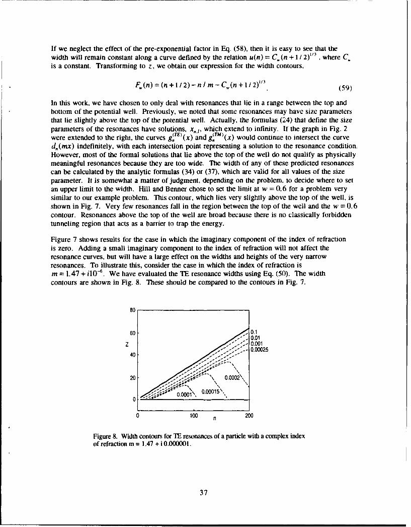
Figure 7 shows results for the case in which the imaginary component of the index of refractionis zero. Adding a small imaginary component to the index of refraction will not affect theresonance curves, but will have a large effect on the widths and heights of the very narrowresonances. To illustrate this, consider the case in which the index of refraction ism = 1.47 + il0-6. We have evaluated the TE resonance widths using Eq. (50). The widthcontours are shown in Fig. 8. These should be compared to the contours in Fig. 7.

80

60 - 0.1"" 0.01

z - 0.0010.00025

40

So.20 u - 0.0002\\,

0 '~' 0.0001\'x 0*00015~0 100 200n

Figure 8. Width contours for TE resonances of a particle with a complex indexof refraction m = 1.47 + i 0.000001.

37

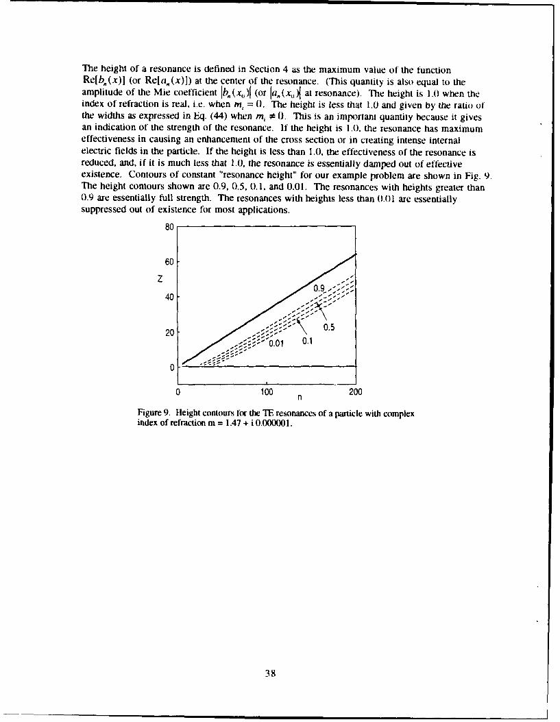
The height of a resonance is defined in Section 4 as the maximum value of the functionRe[b,(x)] (or Re[a,(x)]) at the center of the resonance. (This quantity is also equal to theamplitude of the Mie coefficient Ib, (xj)1 (or Ia,(xA, at resonance). The height is 1.0 when theindex of refraction is real, i.e. when m, = 0. The height is less that 1.0 and given by the ratio ofthe widths as expressed in Eq. (44) when m, * 0. This is an important quantity because it givesan indication of the strength of the resonance. If the height is 1.0. the resonance has maximumeffectiveness in causing an enhancement of the cross section or in creating intense internalelectric fields in the particle. If the height is less than 1.0, the effectiveness of the resonance isreduced, and, if it is much less that 1.0, the resonance is essentially damped out of effectiveexistence. Contours of constant "resonance height" for our example problem are shown in Fig. 9.The height contours shown are 0.9, 0.5, 0.1, and 0.01. The resonances with heights greater than0.9 are essentially full strength. The resonances with heights less than 0.01 are essentiallysuppressed out of existence for most applications.

80

60

z 0

40 -, -

20 ;\ 0.5

20

0 100 200n

Figure 9. Height contours for the TE resonances of a particle with complexindex of refraction m = 1.47 + i 0.000001.

38

6. SUMMARY AND CONCLUDING REMARKS

The analogy between the radial Schrodinger eqlation and the differential equations for theradial Debye potentials has been exploited for the purpose of analyzing electromagneticscattering resonances. These resonances are shown to be analogous to quantum mechanicalshape resonances. The picture developed in this report views these resonances as quasi-boundstates, temporarily trapped in a potential well of the type illustrated in Fig. 1. This viewpointprovides some immediate intuitive insights into the nature of these resonances. For example, thetop and bottom of the potential well determine effective upper and lower bounds for theresonance levels. The resonance widths, which are inversely proportional to the decay time of thequasi-bound state, are determined by the rate at which energy can tunnel through the outerbarrier of the potential well. Since the lower levels must tunnel through a larger barrier the lowerlevels have a longer lifetime and, thus, have narrower widths than the upper levels.

The condition that defines a shape resonance is similar to the condition that defines a bound statein a potential well. This condition states that the wave function must decrease "exponentially" inthe classically forbidden regions outside the well. The application of this boundary conditionleads directly to Eqs. (24a) and (24b). These are the same equations that have been derived inthe theory of morphology-dependent resonances. 1 Figures 3 and 4 show the dramatic changethat occurs in the wave function at resonance. These graphs show how the exponential behaviorof the wave function in the classically forbidden region is responsible for the large electric-fieldamplitudes near the surface of a particle at resonance.

The interpretation of resonances as the quasi-bound states of a potential well can be applied tomore complicated systems than a simple dielectric sphere. We briefly described one such system,a layered sphere with a negative dielectric outer layer. (The potential function for this case isillustrated in Fig. 5.) It is obvious that one can use a similar analysis to consider morecomplicated problems in which the particle has a multilayered structure 21 or a continuouslyvarying index of refraction 22. This approach offers intuitive insights to these more complicatedresonance problems that are not available in the traditional picture, which views a resonance as awave propagating around the sphere, confined by internal reflections. 1

We have also used this analysis to briefly describe the very interesting case of a negative dielectricsphere. This problem is interesting because the system has two distinct types of solutions. Werefer to these as the positive energy (k2 > 0) and negative energy (k2 < 0) solutions. For thepositive energy solution, the potential in the interior of the particle is a repulsive barrier(illustrated in Fig. 6a) that keeps the wave function outside. This is a traditional scatteringproblem that can be calculated by Mie theory. For the negative energy solution, the potentialinside the particle is a deep well (illustrated in Fig. 6b). This case is not a resonance problem, butit is very similar and can be analyzed by the same methods used to study resonances. In this case,the energy cannot tunnel out of the well; therefore, the electromagnetic modes are true boundstates. If it were not for the inevitable internal losses, these states would have an infinite lifetime.These modes exist inside the particle with only a surface evanescent wave penetrating outside ofthe particle.

39

Exact analytic formulas for resonance widths were developed in Section 4. The final useful andsimplified results are contained in the two Eqs. (50) and (55). These formulas predict the widthsof TE and TM resonances, respectively, for both complex (mi * 0) and real (m, = 0) indices ofrefraction. Another useful result of this section is the definition and discussion of thesignificance of the resonance height. The formula for the height is given by Eq. (44).

in Section 5, we presented grapl-ical repescntations that we have found useful for correlating theposition, width (see Figs. 7 and 8), and height data (Fig. 9) for a spectrum of resonances.

40

REFERENCES

1. S. C. Hill and R. E. Benner, "Morphology-dependent resonances," in Optical EffectsAssociated with Small Particles P. W. Barber and R. K. Chang, eds. (World Scientific.Singapore, 1988).

2. P. Chylek, "Particle-wave resonances and the ripple structure in the Mie normalizedextinction cross section," J. Opt. Soc. Am. 66, 285-287 (1976).

3. H.-M. Tzeng, K.F. W-all, M. B. Long, and R. K. Chang, "Laser emission from individualdroplets at wavelengths corresponding to morphology-dependent resonances," Opt. Lett. 9,499-501 (1984).

4. S.-X. Qian, J. B. Snow, H.-M. Tzeng, and R. K. Chang, "Lasing droplets: highlighting theliquid-air interface by laser emission," Science 231, 486-488 (1986).

5. 1. R. Snow, S.-X. Qian and R. K. Chang, "Stimulated Raman scattering from individualwater and ethanol droplets at morphology-dependent resonances," Opt. Lett. 10, 37-39(1985).

6. W. P. Acker, D. H. Leach and R. K. Chang, "Third-order optical sum-frequency generationin micrometer-sized droplets," Opt. Lett. 14, 402-404 (1989).

7. W. P. Acker, A. Serpenguizel, R. K. Chang and S. C. Hill, "Stimulated Raman scattering offuel droplets: chemical concentration and size determination," Appl. Phys. B 51, 9-16(1990).

8. S. Arnold, E. K. Murphy and G. Sager, "Aerosol particle molecular spectroscopy," Appl.Opt. 24, 1048-1053 (1985).

9. L. M. Folan, S. Arnold and S. D. Druger, "Enhanced energy transfer within amicroparticle," Chem. Phys. Lett. 118, 322-327 (1985).

10. S. Arnold, C. T. Liu, W. B. Whitten and J. M. Ramsey, "Room-temperature microparticle-based persistent hole burning memory," Opt. Lett. 16, 420-422 (1991).

11. H. M. Nussenzveig, "Tunneling effects in diffractive scattering and resonances," CommentsAtomic and Molec. Phys. 23, 175-187 (1989).

12. L. G. Guimarles and H. M. Nussenzveig, "Theory of Mie resonances and ripplefluctuations," Optics Commun. 89, 363-369 (1992). (This paper was published after thework for the present report was completed.)

13. C. F. Bohren and D. R. Huffman, Absorption and Scattering of Light by Small Particles(Interscience, New York, 1983).

14. H. C. van de Hulst, Light Scattering by Small Particles (Dover, New York, 1981).

41

15. M. Kerker, The Scattering of Light and Other Electromagnetic Radiation (Academic Press,New York, 1969).

16. C. T. Tai, Dyadic Greens Functions in Electromagnetic Theory (Intext EducationalPublishers, Scranton PA, 1971).

17. P. J. Wyatt, "Scattering of electromagnetic plane waves from inhomogeneous sphericallysymmetric objects," Phys. Rev. 127, 1837-1843 (1962).

18. M. Abramowitz and I. A. Stegun, eds. Handbook of Mathematical Functions (Dover, NewYork, 1965).

19. J. L. Dehmer, "Shape resonances in molecular fields," in Resonances in Electron-MoleculeScattering, van der Waals Complexes, and Reactive Chemical Dynamics, D. G. Truhlar ed.(American Chemical Society, Washington D. C., 1984).

20. J. P. Toennies, W. Wkeiz and G. Wolf, "Observation of orbiting resonances in H2 - rare gasscattering," J. Chem. Phys. 64, 5305-5307 (1976).

21. R. L. Hightower and C. B. Richardson, "Resonant Mie scattering from a layered sphere,"Appl. Opt. 27, 4850-4855 (1985).

22. D. Q. Chowdhury, S. C. Hill and P. W. Barber, "Morphology-dependent Resonances inradially inhomogeneous spheres," J. Opt. Soc. Am. A 8, 1702-1705 (1991).

23. C. Kittel, Introduction to Solid State Physics (Wiley, New York, Fifth edition, 1976).

24. B. A. Hunter, M. A. Box and B. Maier, "Resonance structure ini weakly absorbing spheres,"J. Opt. Soc. Am. A 5, 1281-1286 (1988).

25 G. J. Rosasco and H. S. Bennett, "Internal field resonance structure: Implications for opticalabsorption and scattering by microscopic particles," J. Opt.Soc. Am. 68, 1242-1250 (1978).

26. S. Schiller and R. L. Byer, "High-resolution spectroscopy of whispering gallery modes inlarge dielectric spheres," Opt. Lett. 16, 1138-1140 (1991).

27. 1. R. Probert-Jones, "Resonance component of backscattering by dielectric spheres," J. Opt.Soc. Am. A 1, 822-830 (1984).

42