HAL Id: hal-01166554https://hal.archives-ouvertes.fr/hal-01166554

Submitted on 23 Jun 2015

HAL is a multi-disciplinary open accessarchive for the deposit and dissemination of sci-entific research documents, whether they are pub-lished or not. The documents may come fromteaching and research institutions in France orabroad, or from public or private research centers.

L’archive ouverte pluridisciplinaire HAL, estdestinée au dépôt et à la diffusion de documentsscientifiques de niveau recherche, publiés ou non,émanant des établissements d’enseignement et derecherche français ou étrangers, des laboratoirespublics ou privés.

Velocity measurements based on shadowgraph-likeimage correlations in a cavitating micro-channel flow

Cyril Mauger, Loïc Méès, Marc Michard, Michel Lance

To cite this version:Cyril Mauger, Loïc Méès, Marc Michard, Michel Lance. Velocity measurements based on shadowgraph-like image correlations in a cavitating micro-channel flow. International Journal of Multiphase Flow,Elsevier, 2014, 58, pp.301-312. �10.1016/j.ijmultiphaseflow.2013.10.004�. �hal-01166554�

Velocity measurements based on shadowgraph-like

image correlations in a cavitating micro-channel flow

C. Mauger, L. Mees, M. Michard, M. Lance

Laboratoire de Mecanique des Fluides et d’Acoustique (LMFA), CNRS UMR 5509 –Ecole Centrale de Lyon – INSA de Lyon – Universite Claude Bernard – Lyon 1, Ecully,

France

Corresponding author: Cyril Mauger, tel : 33 (0)4 72 43 61 64, email:cyril.mauger@insa-lyon.fr

Abstract

Cavitation is generally known for its drawbacks (noise, vibration, damage).However, it may play a beneficial role in the particular case of fuel injection,by enhancing atomization processes or reducing nozzle fouling. Studyingcavitation in real injection configuration is therefore of great interest, yettricky because of high pressure, high speed velocity, small dimensions andlack of optical access for instance. In this paper, the authors proposed asimplified and transparent 2D micro-channel (200-400 µm), supplied withtest oil at lower pressure (6 MPa), allowing the use of non-intrusive andaccurate optical measurement techniques. A shadowgraph-like imagingarrangement is presented. It makes it possible to visualize vapor formationsas well as density gradients (refractive index gradients) in the liquid phase,including scrambled grey-level structures connected to turbulence. Thisoptical technique has been already discussed in a previous paper (Maugeret al., 2012), together with a Schlieren and an interferometric imagingtechnique. In this paper, the grey-level structures connected with turbulenceare considered more specifically to derive information on flow velocity. Thegrey-level structure displacement is visualized through couples of imagesrecorded within a very short time delay (about 300 ns). At first, space andspace-time correlation functions are calculated to characterize the evolutionof grey-level structures. Space-time correlations provide structure velocitythat slightly under-estimates the real flow velocity deduced from flowmetermeasurements. Since the grey-level structures remain correlated in time,a second velocity measurement method is applied. An image correlation

Preprint submitted to Int. J. of Multiphase flow September 9, 2013

algorithm similar to those currently used in Particle Image Velocimetry (PIV)is used to extract velocity information, without seeding particles. In additionto the mean velocity of grey-level structures, this second method providesstructure velocity fluctuations. In particular, an increase in structure velocityfluctuations is observed at the channel outlet for a critical normalized lengthof vapor cavities equals to 40-50 %, as expected for the real flow velocityfluctuations. The present study is completed by a parametric study onchannel height and oil temperature. It is concluded that none of themsignificantly impact the critical normalized length for which the fluctuationincrease is observed, even though the magnitude of these fluctuations is largerfor the higher channel.

Keywords: Cavitation, shadowgraph, turbulence, channel flow, correlation,image correlation, Diesel injector

1. Introduction

Over the years, automotive industry standards have increasingly forcedmanufacturers to produce eco-friendly vehicles. During the last decades,heat engines have been improved, becoming less pollutant yet more efficient.The optimization of the thermodynamic cycle has played a key role in theimprovement process. More precisely, increased knowledge of the internalaerodynamics of cylinders and enhanced injection systems have made itpossible to better control fuel evaporation and mixture, and therefore fuelcombustion. Nevertheless, in many respects, the atomization process at theinjector outlet – in particular, the influence of the internal flow on atomization– is still not well understood.

The spray characteristics of Diesel injectors depend on the atomizationprocesses in cylinders, and therefore, they depend on the velocity profileand turbulence inside the nozzle and at the nozzle exit (Birouk and Lekic,2009). The spray characteristics are then likely influenced by the presenceof cavitation in nozzle orifices. Using a backlit micro-PIV system in areal size transparent VCO nozzle, Chaves (2008) highlights that cavitationappears at the sharp edge inlet of the injection orifice. Vapor cavitiesextend along the orifice and bubbles seem to collapse in a very deterministicand localized manner. Velocity fields are also measured by using ParticleImage Velocimetry (PIV). However, the introduction of seeding particles inthe flow is potentially problematic: Particles can act as cavitation nuclei

2

and, consequently, modify the conditions of cavitation inception. Differentcavitation regimes are described in the literature, namely no cavitation,developing cavitation, super-cavitation and hydraulic flip (Sou et al., 2007).Most authors (Birouk and Lekic, 2009; Sou et al., 2007; Hiroyasu, 1991;Soteriou et al., 1995; Wu et al., 1995; Hiroyasu, 2000; Tamaki et al., 2001)show that the most favorable regime for spray atomization is super-cavitationwhile hydraulic flip is the worst in this respect (Sou et al., 2007; Hiroyasu,1991; Bergwerk, 1959). It is considered that super-cavitation is reachedwhen the vapor cavity length is 70 to 100 % the orifice length (Sou et al.,2007). In super-cavitation condition, at least two mechanisms are supposedto influence spray formation. Firstly, cavitation may increase flow turbulence(Tamaki et al., 2001; He and Ruiz, 1995) through bubble collapse andpressure waves. Secondly, bubbles may reach the channel outlet and enhancedirectly the liquid jet atomization when they collapse (Sou et al., 2007).In order to provide useful information on the internal flow inside injectionorifices, different experimental setups are presented in the literature. Flowinvestigation in a realistic geometry and real injection conditions is a difficulttask because of high pressure, high velocities, small dimensions, lack ofoptical access and strong unsteadiness. As a result, most experimentalinvestigations are carried out at lower pressure injection, in a simplifiedgeometry and/or in up-scaled orifices. In a large-scale channel, He and Ruiz(1995) measure both cavitating and non-cavitating flows by means of a LaserDoppler Velocimeter (LDV). When cavitation occurs, they notice a differencein the mean streamwise velocity component profile near the inlet and a 10-20 % increase in turbulence intensity behind vapor cavities. In order toinvestigate the relationship between vapor cavity length and turbulence, highspeed visualizations and Particle Image Velocimetry (PIV) measurementsare conducted by Stanley et al. (2008) in an up-scaled, sharp-edged, acrylicnozzle. In super-cavitation regime, vapor bubbles convected through thenozzle exit have a significant influence on the liquid jet structure and enhancethe aerodynamic shear break-up of the jet. Turbulent Kinetic Energy (TKE)is shown to be strongly linked to vapor cavity length inside the nozzle. Souet al. (2007) also use LDV in a 2D up-scaled channel. They suggest that thestrong turbulence induced by the collapse of cavitation clouds near the exitplays a major role in ligament formation. They visualize cavitation in thenozzle and ligament formation at liquid jet interface simultaneously usinga high-speed camera. They find that the formation of a ligament is often(but not systematically) preceded by the collapse of a cavitation cloud at the

3

channel outlet. It seems that the size of a ligament is roughly proportionalto the size of the vapor formation preceding it. However, Sou et al. (2008)report that the formation of ligaments induced by a collapse of bubbles isless observed in a cylindrical configuration than in a channel configuration.This can be explained by the greater difficulty in observing a flow in acylindrical configuration. For that reason, 2D channel configurations arepreferred by some authors to study cavitation formation. Winklhofer et al.(2001) investigate a cavitating flow in a micro-channel with backlit imaging.They measure velocity profiles with a fluorescence tracing method. Velocityprofile measurements show that vapor formation in the channel inlet increasesflow velocities near the liquid-vapor interface. Winklhofer et al. (2001) alsoreconstruct the pressure field inside the channel by means of a Mach-Zehnderinterferometer arrangement. For different cavitation regimes, they comparethe pressure field and hydraulic behavior. They notice that the flow is chokedafter super-cavitation.These studies suggest that the turbulence induced bycavitation plays a major role in spray formation. It is clear that super-cavitation is the most favorable regime to enhance atomization. Furtherinvestigations are required to highlight cavitation/atomization dependency.

Although observing cavitation inside nozzle orifices is a difficult task,experimental data, especially at the nozzle outlet, are needed to enhance ourgeneral knowledge on high pressure injection processes and to provide reliableinitial conditions for numerical simulations (Menard et al., 2007; Gorokhovskiand Herrmann, 2008; Marcer et al., 2008; Lebas et al., 2009). Obtainingquantitative information as velocity profiles is even more complicated.Consequently, a simplified experimental configuration is considered in thispaper. A 2D micro-channel permanent flow is visualized by using ashadowgraph-like imaging setup, based on a backlit illumination and sensitiveto refractive index gradients. This setup has already been used togetherwith alternative imaging techniques to study cavitation inception, underconditions close to those of direct injection in a 400 µm high micro-channel (Mauger et al., 2012). In this paper, couples of shadowgraph-likeimages are considered to perform velocity measurements in a 2D micro-channel, without seeding particles. The experimental setup is presentedin Section 2. Shadowgraph-like images of the channel flow are presentedin Section 3 together with the result of space and space-time correlations.Section 4 is dedicated to the measurement of mean velocities and fluctuations,based on an image correlation algorithm for a channel height between 200µm and 400 µm.

4

2. Experimental setup

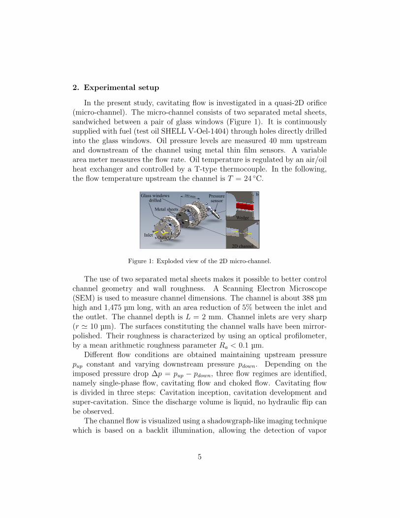
In the present study, cavitating flow is investigated in a quasi-2D orifice(micro-channel). The micro-channel consists of two separated metal sheets,sandwiched between a pair of glass windows (Figure 1). It is continuouslysupplied with fuel (test oil SHELL V-Oel-1404) through holes directly drilledinto the glass windows. Oil pressure levels are measured 40 mm upstreamand downstream of the channel using metal thin film sensors. A variablearea meter measures the flow rate. Oil temperature is regulated by an air/oilheat exchanger and controlled by a T-type thermocouple. In the following,the flow temperature upstream the channel is T = 24 ◦C.

Pressuresensor

Glass windowsdrilled

Metal sheets

InletOutlet

Wedge

b

2D channel

a

180 mm

Figure 1: Exploded view of the 2D micro-channel.

The use of two separated metal sheets makes it possible to better controlchannel geometry and wall roughness. A Scanning Electron Microscope(SEM) is used to measure channel dimensions. The channel is about 388 µmhigh and 1,475 µm long, with an area reduction of 5% between the inlet andthe outlet. The channel depth is L = 2 mm. Channel inlets are very sharp(r ' 10 µm). The surfaces constituting the channel walls have been mirror-polished. Their roughness is characterized by using an optical profilometer,by a mean arithmetic roughness parameter Ra < 0.1 µm.

Different flow conditions are obtained maintaining upstream pressurepup constant and varying downstream pressure pdown. Depending on theimposed pressure drop ∆p = pup − pdown, three flow regimes are identified,namely single-phase flow, cavitating flow and choked flow. Cavitating flowis divided in three steps: Cavitation inception, cavitation development andsuper-cavitation. Since the discharge volume is liquid, no hydraulic flip canbe observed.

The channel flow is visualized using a shadowgraph-like imaging techniquewhich is based on a backlit illumination, allowing the detection of vapor

5

bubbles and cavities, and providing qualitative information on density(refractive index) gradients.

The small size of the channel requires the use of large opticalmagnification. With flow velocities up to 80 m.s−1, an extremely short lightpulse is needed to optically freeze the flow. In addition, an incoherent lightsource is required to avoid speckle on images. Figure 2 presents the opticalarrangement.

tcam

Double pulsed Q-switched

Nd:YAG laser

Red fluorescent

PMMA sheet

Focus lens

set

Collimating

lens set

+

Notch filter

Channel

flow

Zoom optical

systemDouble-frame

CCD cameraImage

frame 1

Image

frame 2

tcam

Figure 2: Shadowgraph-like optical arrangement.

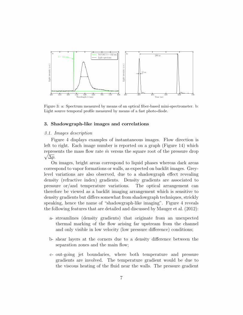
An adequate light source is generated by focusing the second harmonicof a Nd:YAG pulsed laser (wavelength λY AG = 532 nm and pulseduration = 6 ns) on a fluorescent polymethyl-methacrylate (PMMA) sheet.The fluorescent emission is collimated and the remaining laser light is filteredusing a band reject filter (Notch filter λNotch = 533 ± 8 nm). The Nd:YAGdual head laser helps to produce time delayed light pulses. Each incoherentlight pulse lasts 12 ns (FWHM) and has a broad spectrum (Figure 3). Thetime delay between two pulses can be adjusted, down to ∆tmin ' 30 ns.Images are recorded by means of an optical zoom system (OPTEM 125C) on a2048 × 2048 pixels, 10-bit CCD camera. The resulting magnification is about6.4 with a resolution of 1.15 µm.px−1. Using the double-frame mode of thecamera and the dual pulse system of the laser, couples of images separated by∆tcammin ' 200 ns or more are recorded. This optical arrangement permitsthe tracking of rapid events, like bubble dynamics, and the production ofvelocity information.

6

200 300 400 500 600 700Time (ns)

Light

intensity

(a.u.)

12 ns

286 nsb

Figure 3: a: Spectrum measured by means of an optical fiber-based mini-spectrometer. b:Light source temporal profile measured by means of a fast photo-diode.

3. Shadowgraph-like images and correlations

3.1. Images description

Figure 4 displays examples of instantaneous images. Flow direction isleft to right. Each image number is reported on a graph (Figure 14) whichrepresents the mass flow rate m versus the square root of the pressure drop√

∆p.On images, bright areas correspond to liquid phases whereas dark areas

correspond to vapor formations or walls, as expected on backlit images. Grey-level variations are also observed, due to a shadowgraph effect revealingdensity (refractive index) gradients. Density gradients are associated topressure or/and temperature variations. The optical arrangement cantherefore be viewed as a backlit imaging arrangement which is sensitive todensity gradients but differs somewhat from shadowgraph techniques, stricklyspeaking, hence the name of “shadowgraph-like imaging”. Figure 4 revealsthe following features that are detailed and discussed by Mauger et al. (2012):

a- streamlines (density gradients) that originate from an unexpectedthermal marking of the flow arising far upstream from the channeland only visible in low velocity (low pressure difference) conditions;

b- shear layers at the corners due to a density difference between theseparation zones and the main flow;

c- out-going jet boundaries, where both temperature and pressuregradients are involved. The temperature gradient would be due tothe viscous heating of the fluid near the walls. The pressure gradient

7

would be associated to the pressure difference between the out-going jetand the downstream chamber or to local pressure drops inside vorticesgenerated in the jet shear layers;

d- grey-level random-like variations in the wake of the separation zones.They appear as structures developing from the walls to the center ofthe channel where they join together. These grey-level structures areconnected to the turbulence developing in the flow;

e- cavitation inception in the shear layers under the combined effect of thedepression induced by flow detachment at the channel inlet and vorticescaused by instabilities in the shear layers. Mauger et al. (2012) combineseveral optical methods to support this scenario which has also beenobserved in a scale-up configuration (Iben et al., 2011);

f- pressure waves caused by vapor bubble collapse;

g- vapor bubble detachments.

Shadowgraph effects provide an additional amount of information butthey also make image interpretation more difficult, as discussed in Maugeret al. (2012) study. The grey-level random-like variations mentioned aboveare present in most images. These intensity variations are associated todensity (refractive index) variations caused by turbulent structures inside theflow. Although the shadowgraph effects provide information on refractiveindex variations which is integrated along the whole channel depth andessentially qualitative, the grey-level structures are linked to the turbulentstructures convected by the flow. Their displacements are clearly visible froma quick glance at two successive images. In the following, space and space-time correlation functions are used to study these displacements for differentflow conditions.

3.2. Space and space-time correlations

First, image grey-level variations are obtained by subtracting the meanimage of a 50-image series from each image. In the present case, the flowis supposed to be two-dimensional. ψ′ (x, t) is the grey-level variation atposition x and time t. The space-time correlation function at position x andx + ξ is defined by:

8

1

p = 0.45 MPa

Walls

a

Correlation

calculation

6

p = 3.06 MPa

Vapor formation

2

p = 1.49 MPa

Refractive

index gradients

b

7

p = 3.15 MPa

g

3

p = 2.05 MPa

Refractive index

gradient

c

d

8

p = 3.28 MPa

Super-cavitation

4

p = 2.66 MPa

Cavitation inceptionVapor formation

e

9

p = 3.34 MPa

Choked flow

5

p = 2.78 MPa

Pressure waves

f

10

p = 3.47 MPax

y

Figure 4: Examples of instantaneous shadowgraph-like images. The channel height is388 µm. pup = 5.00 MPa, T = 24 ◦C.

9

R (ξ,x,∆t) =〈ψ′ (x, t)ψ′ (x + ξ, t)〉√⟨ψ′ (x, t)2

⟩√⟨ψ′ (x + ξ, t)2

⟩ (1)

where 〈.〉 is the time-averaging operator and ∆t the time delay between twoimages.

3.2.1. Space correlations

The space correlation R (ξ,x,∆t = 0) is first considered. Figure 5adisplays the iso-contours of the space correlation function calculated in theflow region shown in image number 1 of Figure 4, but for ∆p = 2.71 Mpa.A correlation peak is clearly visible in the center of the map. An integrallength scale based on density fluctuations corresponding to R (ξ,x,∆t = 0)can be defined as:

Ln (x) =

∫ ∞

0

R (ξ,x,∆t = 0) dξ (2)

An integral length scale can be deduced for the streamwise direction(Lnx) or the cross-streamwise direction (Lny). In practice, the calculationof the integral length scale cannot extend to infinity. It is then interruptedwhen a zero value is achieved. Convergence is hardly obtained with only 50images. The noise that can be seen in Figure 5a accounts for the apparentlack of statistics. At channel outlet, the turbulence is assumed to be locallyhomogeneous. In order to increase the statistical convergence of R (ξ,x,∆t),the correlation function is calculated for pixels located close to the initialpoint, i.e. for pixels in a 11 × 11 pixel square, centered on the initial pixel.An example of space correlation function averaged over 121 points is shownin Figure 5b. The positive iso-values of the space correlation function arealmost circular, showing a quasi-isotropic pattern. This observation is in linewith the results obtained by Kim and Hussain (1992) for space-correlationsbased on pressure fluctuations in a fully established channel flow.

In Figure 6, the integral length scales Lnx and Lny are plotted againstthe Reynolds number Re, from low pressure drop condition (lower Re) tosuper-cavitation (higher Re). The Reynolds number is defined as:

Re =ρUMDh

µ(3)

10

Figure 5: Iso-contours of the space corre1ation function R (ξ,x,∆t = 0) at the channeloutlet centerline (0.9L). pup = 5.00 MPa, ∆p = 2.71 MPa , T = 24 ◦C. a: Single pointcorrelation. b: Correlation function averaged over 121 points.

Figure 6: Evolution of the integral length scales Lnx and Lny versus the Reynolds numberRe at the channel outlet centerline (0.9L). pup = 5.00 MPa, T = 24 ◦C.

where ρ and µ are the density and the dynamic viscosity of the test oil,respectively. The values of these parameters are given by Ndiaye et al. (2012)as a function of temperature and pressure. Dh is the hydraulic diameter ofthe channel and UM the mean velocity inside the channel.

The same averaging method as the one described above is used to increasethe level of statistical convergence for Lnx and Lny. In Figure 6, the integrallength scale Lnx decreases with increasing Reynolds number until cavitationinception. In the cross-streamwise direction, Lny remains almost constant.Once cavitation appears, Lnx and Lny seem to slightly increase. For greatervalues of the Reynolds number, in the super cavitation regime, the presenceof cavitation in the region of interest (ROI) does not allow the correlationcalculation.

To go further in the analysis, grey-level structures are now investigated

11

10−2 10−1 100

k/2π (µm−1)

105

106

107

108

109

1010

1011

1012

Eψ′(k)

∆p = 0.99 MPa

∆p = 1.49 MPa

∆p = 1.96 MPa

∆p = 2.66 MPa∗

∆p = 2.78 MPa

∆p = 2.84 MPa

∆p = 2.90 MPa

∆p = 3.06 MPa

Figure 7: Grey-level variation spectrum for different flow conditions. ∗Cavitationinception. pup = 5.00 MPa, T = 24 ◦C.

by using a two-dimensional discrete Fourier transform. The two-dimensionalenergy spectrum ∆ (k) of the grey-level variation is defined as:

∆ (k) =

(2π

a

)2

|Ψ′ (k)|2 (4)

where Ψ′ (k) is the Fourier transform of the grey-level variation ψ′ (x) and athe ROI. Grey-level variations are assumed to be statistically homogeneousand isotropic, ∆ (k) = ∆ (k). It is then useful to define another spectralfunction Eψ′ (k), which is the radial average of the two-dimensional spectrum∆ (k), multiplied by a factor 2πk:

Eψ′ (k) = 2πk∆ (k) =

∫ 2π

0

∆ (k, φ) kdφ (5)

The ROI is a square of 256 × 256 pixels (' 295 µm2) located atthe channel outlet. To reduce aliasing due to ROI boundaries, a Hannwindow function is applied. Examples of spectra are given in Figure 7 fordifferent flow conditions. From single-phase flow to cavitation inception (from∆p = 0.99 MPa to ∆p = 2.66 Mpa), the spectra slightly move toward smallerstructures (white arrow) and larger structures increase. After cavitationinception (∆p ≥ 2.78 MPa), spectrum distributions superimpose at smallscales when the largest scales increase faster than before cavitation inception(black arrow). The occurrence of cavitation seems to have an influence onthe evolution of integral length scales and on grey-level variation spectra.However, these behaviors have no obvious interpretation (not even for low∆p before cavitation inception) and it is not clear yet if the behavior of the

12

−40

−20

0

20

40

y(µ

m)

a

∆p = 1.49 MPa

b

∆p = 2.05 MPa

c

∆p = 2.66 MPa

∆t=

0n

s

d

∆p = 3.06 MPa

−40 −20 0 20 40

x (µm)

−40

−20

0

20

40

y(µ

m)

e

−40 −20 0 20 40

x (µm)

f

−40 −20 0 20 40

x (µm)

g

−40 −20 0 20 40

x (µm)

h

∆t=

28

6n

s

−0.8

−0.6

−0.4

−0.2

0.0

0.2

0.4

0.6

0.8

Figure 8: Iso-contours of the space-time correlation functions R (ξ,x,∆t = 0 ns) andR (ξ,x,∆t = 286 ns) at the channel exit centerline 0.9L. pup = 5.00 MPa, T = 24 ◦C.a and e: ∆p = 1.49 MPa, b and f: ∆p = 2.05 MPa, c and g: ∆p = 2.66 MPa, d and h:∆p = 3.06 MPa.

grey-level structures can be directly linked to turbulent flow characteristics,such as pressure or density spectra. In the following, the displacement ofthe grey-level structures will be investigated through space-time correlationcomputations.

3.2.2. Space-time correlations

A quick glance at two successive images of the flow, recorded within ashort time ∆t (less than 300 ns), shows a clear displacement of the grey-levelstructures. Space-time correlation functions are now considered to determinewhether this displacement can be used to obtain velocity information of theflow. In this paper, only one value of ∆t is considered (∆t = 286 ns),which does not allow one to study the flow in terms of turbulence time scale.Nevertheless, the space-time correlation function for ∆t = 286 ns can beused to estimate an advection velocity of the turbulent structures. Examplesof space-time correlations R (ξ,x,∆t = 0 ns) and R (ξ,x,∆t = 286 ns) aregiven in Figure 8 for different flow conditions inside the channel at streamwiselocation x/L = 0.9L.

Figure 8 displays examples of correlation functions for ∆t = 0 ns(Figure 8a-d) and ∆t = 286 ns (Figure 8e-h), computed from a sample ofimages (or image couples) recorded in four different flow conditions (∆p).In each case, the correlation function for ∆t = 286 ns is similar to the one

13

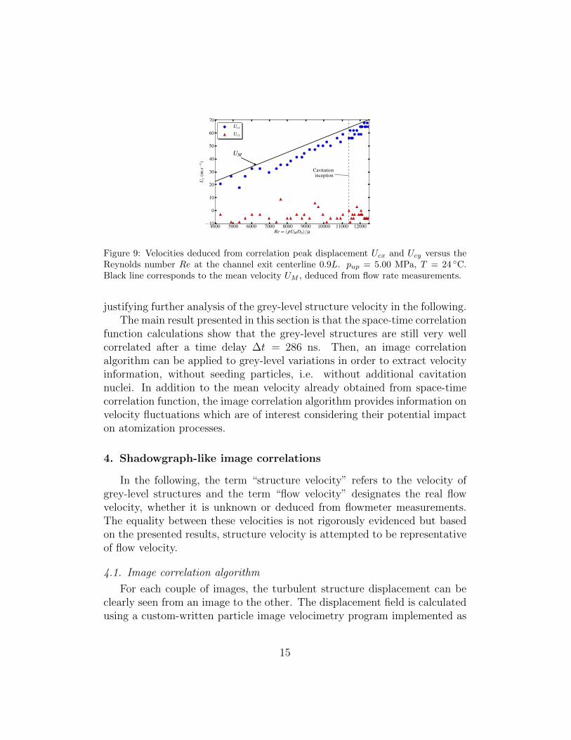
for ∆t = 0 ns, but correlation peaks are clearly shifted, mainly in the meanflow direction. The peaks are also slightly attenuated but their displacementcan be easily quantified by a separation vector ξc from which a grey-levelstructure advection velocity Uc = ξc/∆t can be defined. No spatial averagingsimilar to the one applied in Figure 5b is required to extract this advectionvelocity. In Figure 8, the structure displacement increases with the pressuredrop. Figure 9 shows the structure advection velocity deduced from a largersample of images. The streamwise and cross-streamwise components of thegrey-level structure advection velocity Ucx and Ucy are plotted against theReynolds number based on the mean velocity UM deduced from flow ratemeasurements. The cross-streamwise velocity component remains almostconstant and close to zero. The streamwise velocity component increaseslinearly with the Reynolds number, as expected. Ucx is close to the meanvelocity UM deduced from flow rate measurements and represented by theblack line in Figure 9. Ucx is however lower than UM by about 10%, inthe whole range of measurement. Several explanations can be proposed toaccount for this discrepancy. It is assumed that the grey-level structuresare connected to turbulence through density variations and a shadowgrapheffect. Firstly, the advection velocity of the turbulent structures couldbe lower than the flow velocity. Secondly, the grey-level structures couldmove at a lower velocity than the turbulent structures. The shadowgrapheffect being integrated along the whole depth of the channel (along lightray paths, perpendicular to images), it could be more sensitive to densityvariations, in particular flow areas for example – in the boundary layers nearthe glass windows, where the velocity is lower. The discrepancy could alsobe attributed to the flow rate measurement which is performed upstreamthe channel. The sealing of the channel is achieved by a direct glass/metalcontact to avoid unwanted cavitation formations, due to the use of glue forexample. The sealing may not be perfect and a part of the flow could bediverted outside the channel, between the glass windows and the metal sheets.Finally, the mean grey-level structure velocities presented in Figure 9 havebeen obtained from a flow area located in the channel centerline, as shownin Figure 4-1. Later in the paper, in Section 4.2, a possible bias in structurevelocity measurement in the centerline of the channel will be discussed. Fromthe results presented in this paper, the equivalence between the grey-levelstructure velocity and the real flow velocity cannot be rigorously evidenced.However, the behavior of the mean velocity measured from the grey-levelstructures is consistent with what is expected for the real flow velocity,

14

4000 5000 6000 7000 8000 9000 10000 11000 12000Re = (ρUMDh)/µ

−10

0

10

20

30

40

50

60

70

Uc

(m.s−

1)

Cavitationinception

UM

Ucx

Ucy

Figure 9: Velocities deduced from correlation peak displacement Ucx and Ucy versus theReynolds number Re at the channel exit centerline 0.9L. pup = 5.00 MPa, T = 24 ◦C.Black line corresponds to the mean velocity UM , deduced from flow rate measurements.

justifying further analysis of the grey-level structure velocity in the following.The main result presented in this section is that the space-time correlation

function calculations show that the grey-level structures are still very wellcorrelated after a time delay ∆t = 286 ns. Then, an image correlationalgorithm can be applied to grey-level variations in order to extract velocityinformation, without seeding particles, i.e. without additional cavitationnuclei. In addition to the mean velocity already obtained from space-timecorrelation function, the image correlation algorithm provides information onvelocity fluctuations which are of interest considering their potential impacton atomization processes.

4. Shadowgraph-like image correlations

In the following, the term “structure velocity” refers to the velocity ofgrey-level structures and the term “flow velocity” designates the real flowvelocity, whether it is unknown or deduced from flowmeter measurements.The equality between these velocities is not rigorously evidenced but basedon the presented results, structure velocity is attempted to be representativeof flow velocity.

4.1. Image correlation algorithm

For each couple of images, the turbulent structure displacement can beclearly seen from an image to the other. The displacement field is calculatedusing a custom-written particle image velocimetry program implemented as

15

an ImageJ plugin (http://rsb.info.nih.gov/ij) by Tseng et al. (2012).The package of PIV software is available at https://sites.google.com/

site/qingzongtseng/piv. The displacement field is performed through aniterative scheme. The spacing between each interrogation window for thelast pass is 12 px, resulting in a final grid size for the displacement fieldof 14 µm × 14 µm. The image processing makes it possible to determinestructure displacement in the whole channel with the exception of zoneswhere walls or vapor formations are present.

A data post-processing is required to eliminate erroneous displacementvectors due to zones that are free from structures. The post-processingis applied when the standard deviation of grey-levels in an interrogationwindow (12 px × 12 px) is below a critical value – typically 5. It mayhappen that this threshold method removes vectors that should be preserved.If so, a new vector is calculated from the neighbor vectors when they arenot equal to zero. The quantity of vectors recalculated is about 3 % ofthe total number of vectors. Channel dimensions are well known thanksto SEM visualizations and the time delay between two light pulses hasbeen accurately measured with a fast photodiode. The velocity field of theturbulent structures can therefore be reconstructed. Figure 10 presents aschematic of image processing and post-processing.

tcam = 286 ns

1st pass

2nd pass

3rd pass

a b

Elimination of

erroneous

displacement

vectors

Displacement

(px)

Velocity

(m.s-1)

Conversion into

velocity

Figure 10: Schematic of image processing (a) (Tseng et al., 2012) and post-processing (b).

The image processing is applied to series of 50 images recorded in the sameconditions. For each series, the mean structure velocity 〈Uψ′〉 and root meansquare (RMS) of structure velocity are calculated. No structure velocity canbe obtained in zones that are free from structures and in those with vaporformations. For a given zone, the images from which no velocity is obtained

16

are not taken into account in the mean and RMS calculations. Also, meanvelocity and RMS are ignored when they are based on a sample smallerthan 10 (velocity information deduced from less than 20 % of all images).An example of partial structure velocity field combined with probability ofcavitation occurrence is shown in Figure 11.

50 m.s−1

0 10 20 30 40 50 60 70 80 90 100

Figure 11: Probability of cavitation occurrence combined with partial structure velocityfield. pup = 5.00 MPa, ∆p = 3.06 MPa, T = 24 ◦C.

Since vapor cavities develop in the channel as the pressure differenceincreases, velocity information is not taken into account either when theprobability of cavitation occurrence is higher than 50 % in the ROI.

4.2. Structure velocity profiles

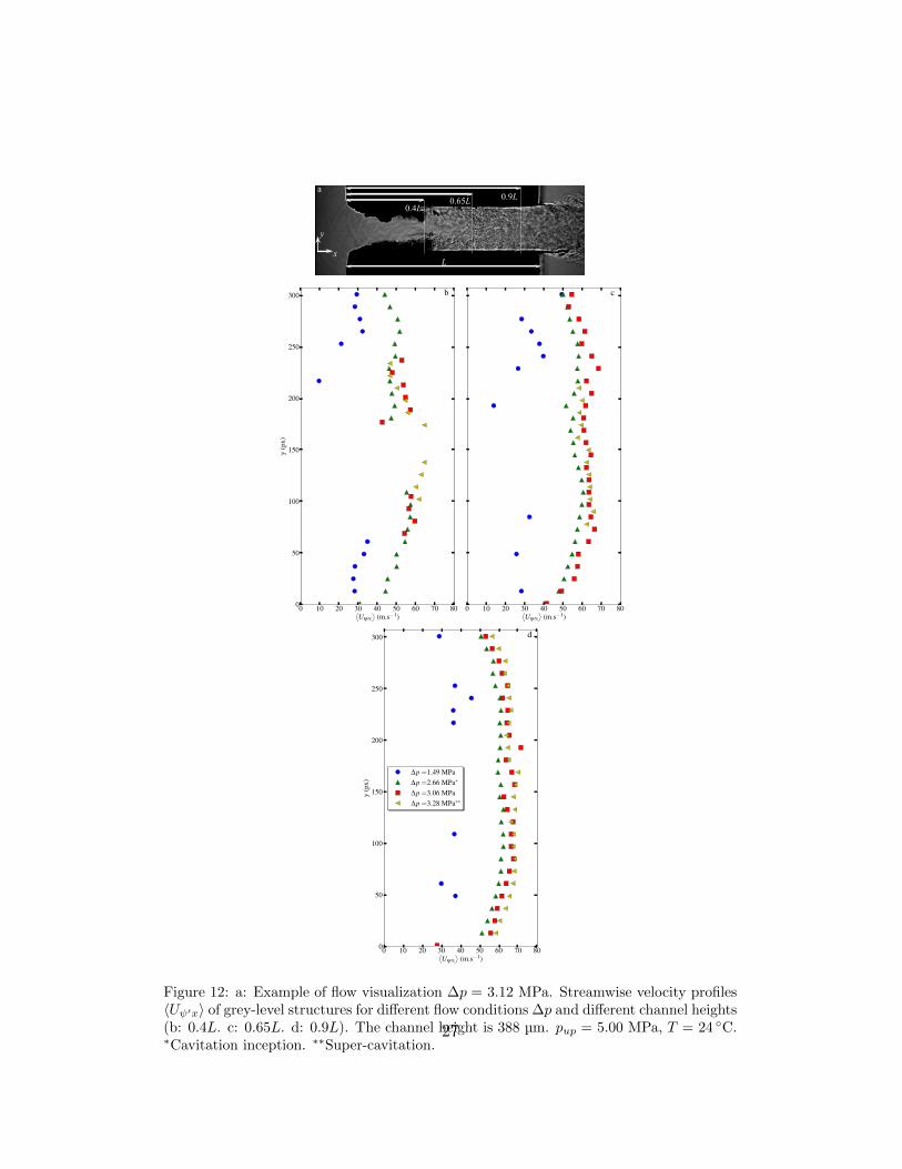
Figure 12 shows streamwise structure velocity profiles 〈Uψ′x〉 averagedover a series of images at different locations inside the channel (0.4L, 0.65Land 0.9L). The profiles at 0.4L are incomplete because structures are notpresent through the whole height of the channel at this location. Closer to thechannel inlet, for x < 0.4L, no structure velocity measurement is performedbecause of limited statistics (few structures).

At 0.4L (Figure 12b), a global increase in structure velocity withincreasing ∆p is observed, as expected. The velocity information is onlypartial at this location. Near the centerline, the profiles are cut-off in theabsence of structures. For ∆p = 3.06 MPa and ∆p = 3.28 MPa, the edges ofprofiles are also cut-off due to the presence of vapor cavities near the walls.

At 0.65L and 0.9L (Figure 12c-d), the profiles are almost flat. The profilesfor ∆p = 1.49 MPa are also incomplete at these locations, due to the lack ofstructures. A structure velocity deficit is noticed at the center of the profilefor ∆p = 3.06 MPa. At these locations, the two boundary layers merge,possibly leading to a deformation of the structures within the time delaybetween the two images, which may bias the structure velocity measurements.

17

At 0.9L, the profiles for ∆p = 3.06 MPa and ∆p = 3.28 MPa are quite similar,testifying of the imminence of the choked flow.

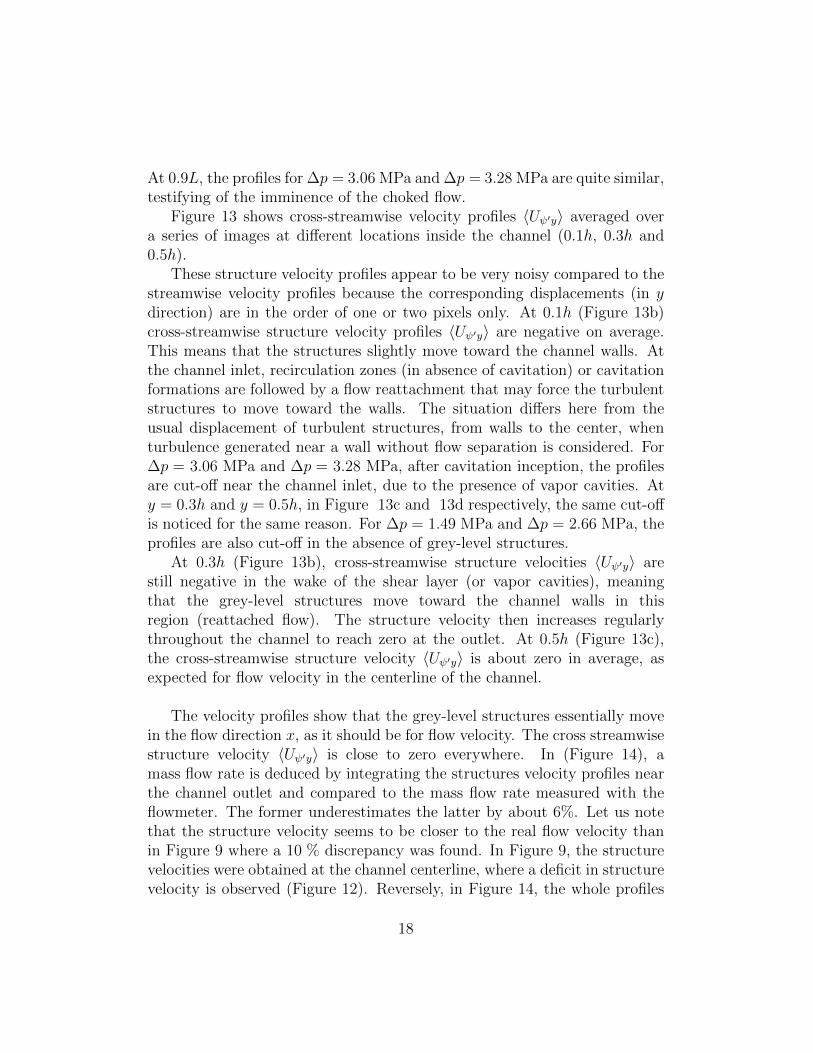
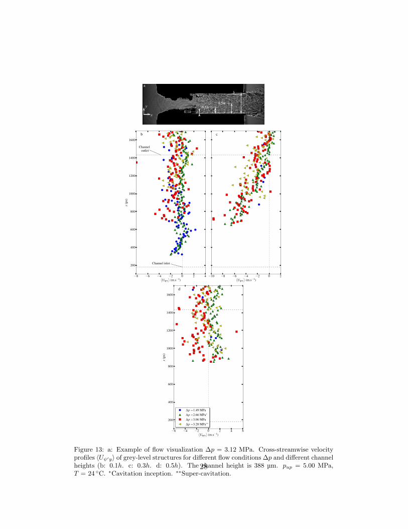
Figure 13 shows cross-streamwise velocity profiles 〈Uψ′y〉 averaged overa series of images at different locations inside the channel (0.1h, 0.3h and0.5h).

These structure velocity profiles appear to be very noisy compared to thestreamwise velocity profiles because the corresponding displacements (in ydirection) are in the order of one or two pixels only. At 0.1h (Figure 13b)cross-streamwise structure velocity profiles 〈Uψ′y〉 are negative on average.This means that the structures slightly move toward the channel walls. Atthe channel inlet, recirculation zones (in absence of cavitation) or cavitationformations are followed by a flow reattachment that may force the turbulentstructures to move toward the walls. The situation differs here from theusual displacement of turbulent structures, from walls to the center, whenturbulence generated near a wall without flow separation is considered. For∆p = 3.06 MPa and ∆p = 3.28 MPa, after cavitation inception, the profilesare cut-off near the channel inlet, due to the presence of vapor cavities. Aty = 0.3h and y = 0.5h, in Figure 13c and 13d respectively, the same cut-offis noticed for the same reason. For ∆p = 1.49 MPa and ∆p = 2.66 MPa, theprofiles are also cut-off in the absence of grey-level structures.

At 0.3h (Figure 13b), cross-streamwise structure velocities 〈Uψ′y〉 arestill negative in the wake of the shear layer (or vapor cavities), meaningthat the grey-level structures move toward the channel walls in thisregion (reattached flow). The structure velocity then increases regularlythroughout the channel to reach zero at the outlet. At 0.5h (Figure 13c),the cross-streamwise structure velocity 〈Uψ′y〉 is about zero in average, asexpected for flow velocity in the centerline of the channel.

The velocity profiles show that the grey-level structures essentially movein the flow direction x, as it should be for flow velocity. The cross streamwisestructure velocity 〈Uψ′y〉 is close to zero everywhere. In (Figure 14), amass flow rate is deduced by integrating the structures velocity profiles nearthe channel outlet and compared to the mass flow rate measured with theflowmeter. The former underestimates the latter by about 6%. Let us notethat the structure velocity seems to be closer to the real flow velocity thanin Figure 9 where a 10 % discrepancy was found. In Figure 9, the structurevelocities were obtained at the channel centerline, where a deficit in structurevelocity is observed (Figure 12). Reversely, in Figure 14, the whole profiles

18

are integrated to derive a flow rate, minimizing the effect of this deficit on theresults. The difference between flow rates deduced from structure velocityprofiles and measured by flow meter is bigger for the largest pressure dropconsidered in the Figure 14, when the flow is choked (

√∆p ≥ 1.82 MPa0.5).

In choked flow condition, the occurrence of vapor cavities at the channeloutlet increases, reducing the statistical reliability of the results. In addition,pressure waves associated to bubble collapses take part in the grey-levelstructures and probably distort the image correlation result or the grey-levelstructures themselves.

The experimental setup presented here does not make it possible to studythe influence of the internal flow on spray formation because the dischargevolume is liquid. Nevertheless, structure velocity fluctuations at the channeloutlet can be investigated depending on flow conditions.

4.3. Structure velocity fluctuations

In Section 4.2, velocity information on advected grey-level structures hasbeen obtained from shadowgraph-like images by using an image correlationalgorithm. At the channel outlet, the measured structure velocities areconsistent with the flowmeter measurements (Figure 14). It is then assumedthat structure velocities are representative of real flow velocities and resultsare further analyzed in this section to extract structure velocity fluctuations.These fluctuations are derived from the flow area delimited by white dashesin Figure 15. The root mean squares of structure velocity σx and σy as well asthe mean streamwise structure velocity 〈Uψ′x〉, are first averaged in space over

this area leading to σx, σy and 〈Uψ′x〉 respectively. Relative fluctuations arethen considered through the ratios ςx and ςy between the averaged root meansquares of structure velocity and the averaged streamwise mean structurevelocity, that is

ςx = σx

/〈Uψ′x〉 and ςy = σy

/〈Uψ′x〉 (6)

The streamwise and cross-streamwise structure velocity fluctuations areplotted against the Reynolds number in Figure 16a. The Reynolds numberis not based on the structure velocity 〈Uψ′x〉 resulting from image correlationbecause this velocity measurement is not reliable in choked flow condition,as mentioned in the previous section. The Reynolds number is based on themean velocity UM deduced from the flow rate measurements. In Figure 16a,the streamwise and cross-streamwise fluctuations evolve similarly but ςy is

19

lower than ςx. From Re = 5,000 to 12,000, the relative root mean square ofstructure velocity increases slowly for both streamwise and cross-streamwisedirections. ςx and ςy raise from 7 to 10 % and from 5 to 7 %, respectively. ForRe > 12,000 and until the choked flow regime, ςx leaps by more than 34 %and ςy by more than 38 %. The sudden rise of structure velocity fluctuationsdoes not occur at cavitation inception but for Re = 12,000 when cavitationis already well developed in the channel.

It is common practice to introduce an dimensionless cavitation numberwhen studying a cavitating flow. In Figure 16b, ςx and ςy are plotted againstthe cavitation number KN defined by Nurick (1976) as:

KN =pup − psat

∆p(7)

where psat is the saturated vapor pressure of the test oil which isapproximately equal to 10 Pa (Chorazewski et al., 2012). psat can thereforebe disregarded. Figure 16b (right to left for decreasing KN) does not help usto better distinguish fluctuations in regards of developing cavitation insidethe channel. Nevertheless, the sudden rise seems to appear for KN = 1,7.

A practical way of analyzing cavitation influence on velocity fluctuationsis to plot ςi versus the normalized length of vapor cavities lnorm (lcav/L). lcav isobtained from a series of images at each flow condition. On shadowgraph-likeimages, vapor appears in dark and liquid in grey-level variations depending onrefractive index gradients. To eliminate refractive index gradients, segmentedimages are obtained by applying a threshold. Structure velocity fluctuationsare plotted against the normalized cavity length lnorm in Figure 16c, fromcavitation inception to choked flow condition. Structure velocity fluctuationsincrease slowly from cavitation inception (lowest values of lnorm) to lnormequal to about 40-50 %. A more significant increase of fluctuations isobserved for lnorm ≥ 50 %. Thus, velocity fluctuations at the channel outletseem to be strongly affected by cavitation as soon as the vapor cavities reachthe middle of the channel. This suggests that, in a real injector configuration,vapor formation may start to improve fuel atomization by increasing velocityfluctuations at this stage of cavitation development. Nevertheless, thishypothesis cannot be confirmed by the present experimental setup sinceit does not produce any spray (liquid volume discharge). Super-cavitationregime is known as the regime for which vapor cavities and bubbles reachthe end of the channel. It is sometimes defined as the regime from whichcavitation starts to improve atomization processes, even if the related

20

mechanisms are not well highlighted (increase in turbulence Tamaki et al.(2001); He and Ruiz (1995) or interface deformation Sou et al. (2007) inducedby bubble collapses). In Sou et al. study Sou et al. (2007), the startingpoint of super-cavitation regime is associated to a normalized cavity lengthlnorm ' 70 %, that is a significantly larger value than the one suggestedby Figure 16c. The starting point could be explained by the up-scaledconfiguration studied in Sou et al. (2007) or by a gap between the startingpoint of structure velocity fluctuation enhancement and that of a significanteffect in atomization efficiency (or change in spray angle). In the following,channel height has been modified in order to know if it affects structurevelocity fluctuations at the outlet.

4.4. Channel height influence on outlet structure velocity fluctuations

Changing channel height without modifying other parameters is a difficulttask. Indeed, cavitation is very sensitive to small geometric modifications,especially at the channel inlet. A small change in the inlet radius or thepresence of a defect at this point can dramatically influence cavitationinception. In order to keep the same inlet geometry, the different channelsare constructed with the same pair of metal sheets. The space between thetop sheet and the bottom sheet is modified by means of wedges in papergasket placed between the metal sheets (Figure 1b). The use of paper gasketensures the sealing of the metal sheets. As the paper gasket is compressible,it is not possible to precisely predict the height of the channel. The geometryof the different channels is therefore measured a posteriori by a SEM. Threedifferent channel heights are obtained, namely 238, 322 and 388 µm. Thestreamwise and cross-streamwise relative root mean squares of structurevelocity are calculated in the same way as explained in Section 4.3 for thethree different channels in a flow area of 60 px × 60 px, 80 px × 80 px and96 px × 96 px, respectively.

Figure 17 presents the structure velocity fluctuations ςx and ςy versuslnorm for different channel heights. The higher the channel, the moresignificant the velocity fluctuations. The increase in structure velocityfluctuations is significant in the cross-streamwise direction, suggesting ananisotropy of the turbulent flow. The channel height has no influence on thecritical length lnorm at which fluctuations increase suddenly: for the threechannel heights and both directions, this critical length is still lnorm = 40-50 %. The turbulence induced by cavitation seems to be more developed in

21

higher nozzles, but the critical normalized cavity length defining the super-cavitation regime starting point seems to be independent of the channelheight, in the size range considered here. The effect of a complete scale-up (including the channel length) has not been considered.The potential effect of temperature on structure velocity fluctuations hasbeen investigated for flow temperatures varying between 20 ◦C and 50 ◦C.The results are not detailed in this paper because no significant effect hasbeen observed within this temperature range.

5. Conclusion

Shadowgraph-like imaging can be used to investigate a cavitating flowin a micro-channel. This optical technique provides a wealth of informationon the flow, allowing one to distinguish vapor and liquid phases, providingqualitative information on density gradients in the liquid phase. In particular,grey-level random-like structures are visible in regions when and for flowconditions where turbulence is expected. These structures are likely relatedto density fluctuations of the turbulent flow. Although their connectionwith the turbulent structures is not rigorously established, the grey-levelstructures have been studied by using space-time correlations and spectralanalysis. In single-phase flow condition (for low pressure drop from upstreamto downstream of the channel), the integral length scale deduced fromthe space-correlation of the grey-level structures decreases with increasingReynolds number (or pressure drop). At cavitation inception, it stopsdecreasing and increases slowly. A Fourier transform analysis of thesestructures shows a spectrum enlargement with increasing Reynolds number.Before cavitation inception, the spectra are essentially shifted toward smallscales when the largest scales increase slowly. After cavitation inception,a more significant growth rate of the largest scales is observed, suggestinga production of large scale turbulent structures induced by cavitation– although, as indicated above, the connection between the grey-levelstructures and turbulence is not rigorously established yet. The mostimportant results provided by the space-time correlation analysis of theshadowgraph-like images is that grey-level structures remain correlatedbetween two images recorded at 300 ns delay. Advection velocities of thestructures are then deduced from space-time correlations. These structurevelocities are close to the velocities deduced from flow rate measurements.In addition, an image correlation algorithm, similar to those currently

22

employed in Particle Image Velocimetry (PIV), can be applied to couplesof shadowgraph-like images to obtain mean velocity fields as well as velocityfluctuations in the channel flow. The main advantage of this technique isthat it does not use seeding particles which could act as cavitation nucleiand modify the flow behavior. The structure velocity fields obtained areonly partial as on the one hand, the presence of grey-level structures isrequired to extract velocity information and, on the other hand, velocitycannot be measured in flow areas where vapor cavities are fully developed.However, mean structure velocity profiles have been measured in variousflow sections. The flow rate deduced from these profiles near the channelexit are consistent with the flowmeter measurement, with a nearly constantdeviation in the order of 5 % from low pressure drop conditions to choked flowcondition for which larger deviations are observed. Assuming that the grey-level structure velocity is representative of the real flow velocity, structurevelocity fluctuations have been also evaluated as a function of the pressuredrop from upstream to downstream of the channel. The relative structurevelocity fluctuation increases slowly with increasing Reynolds number insingle-phase conditions and also after cavitation inception, until the super-cavitation regime for which a fast increase in the fluctuation growing rate isobserved. The critical cavity length defining the starting point of the super-cavitation regime is evaluated to be about half the channel height (lnorm ' 40-50 %). This value is smaller than the one reported in Sou et al. (2007) study(lnorm ' 70 %) for a similar but up-scaled configuration. Variations of thechannel height (between 238 µm and 388 µm) and flow temperature (between20 ◦C and 50 ◦C) have also been investigated. No significant temperatureeffects have been observed. Greater relative structure velocity fluctuationshave been found in higher channels but the critical length associated to super-cavitation regime does not change in the considered range of channel heights.

Acknowlegments

This work takes place in the French collaborative program NADIA-bio (New Advance Diesel Injection Diagnosis for bio fuels). This programis supported by the French Automotive Cluster Mov’eo, and funded bythe DGCIS (Direction Generale de la Competitivite, de l’Industrie et desServices), the Region Haute Normandie and the Conseil General des Yvelines.

Bergwerk, W., 1959. Flow pattern in diesel nozzle spray holes. Proceedings of

23

the Institution of Mechanical Engineers 1847-1982 (vols 1-196) 173 (1959),655–660.

Birouk, M., Lekic, N., 2009. Liquid jet breakup in quiescent atmosphere: Areview. Atomization and Sprays 19 (6), 501–528.

Chaves, H., 2008. Particle image velocimetry measurements of the cavitatingflow in a real size transparent VCO nozzle. In: ILASS 2008.

Chorazewski, M., Dergal, F., Sawaya, T., Mokbel, I., Grolier, J., Jose,J., 2012. Thermophysical properties of normafluid (iso 4113) over widepressure and temperature ranges. Fuel.

Gorokhovski, M., Herrmann, M., 2008. Modeling primary atomization. Annu.Rev. Fluid Mech. 40, 343–366.

He, L., Ruiz, F., 1995. Effect of cavitation on flow and turbulence in plainorifices for high-speed atomization. Atomization and Sprays 5 (6), 569–584.

Hiroyasu, H., 1991. Break-up length of a liquid jet and internal flow in anozzle. ICLASS-91, 275–282.

Hiroyasu, H., 2000. Spray breakup mechanism from the hole-type nozzle andits applications. Atomization and Sprays 10 (3-5), 511–527.

Iben, U., Morozov, A., Winklhofer, E., Wolf, F., 2011. Laser-pulseinterferometry applied to high-pressure fluid flow in micro channels.Experiments in fluids 50 (3), 597–611.

Kim, J., Hussain, F., 1992. Propagation velocity and space-time correlationof perturbations in turbulent channel flow. NASA STI/Recon TechnicalReport N 93, 25082.

Lebas, R., Menard, T., Beau, P., Berlemont, A., Demoulin, F.-X., 2009.Numerical simulation of primary break-up and atomization: Dns andmodelling study. International Journal of Multiphase Flow 35 (3), 247–260.

Marcer, R., Dassibat, C., Argueyrolles, B., 2008. Simulation of two-phaseflows in injectors with the cfd code eole.

24

Mauger, C., Mees, L., Michard, M. Azouzi, A., Valette, S., 2012.Shadowgraph, schlieren and interferometry in a 2d cavitating channel flow.Experiment in Fluids 53, 1895–1913.

Menard, T., Tanguy, S., Berlemont, A., 2007. Coupling level set/vof/ghostfluid methods: Validation and application to 3d simulation of the primarybreak-up of a liquid jet. International Journal of Multiphase Flow 33 (5),510–524.

Ndiaye, E., Bazile, J., Nasri, D., Boned, C., Daridon, J., 2012. High pressurethermophysical characterization of fuel used for testing and calibratingdiesel injection systems. Fuel.

Nurick, W., 1976. Orifice cavitation and its effect on spray mixing. Journalof fluids engineering 98, 681.

Soteriou, C., Andrews, R., Smith, M., 1995. Direct injection diesel spraysand the effect of cavitation and hydraulic flip on atomization. Tech. rep.,Society of Automotive Engineers, 400 Commonwealth Dr, Warrendale, PA,15096, USA,.

Sou, A., Hosokawa, S., Tomiyama, A., 2007. Effects of cavitation in a nozzleon liquid jet atomization. International journal of heat and mass transfer50 (17), 3575–3582.

Sou, A., Maulana, M., Hosokawa, S., Tomiyama, A., 2008. Ligamentformation induced by cavitation in a cylindrical nozzle. Journal of FluidScience and Technology 3 (5), 633–644.

Stanley, C., Rosengarten, G., Milton, B., Barber, T., 2008. Investigationof cavitation in a large-scale transparent nozzle. University of New SouthWales, Australia, F.

Tamaki, N., Shimizu, M., Hiroyasu, H., 2001. Enhancement of theatomization of a liquid jet by cavitation in a nozzle hole. Atomizationand Sprays 11 (2), 125–137.

Tseng, Q., Duchemin-Pelletier, E., Deshiere, A., Balland, M., Guillou, H.,Filhol, O., Thery, M., 2012. Spatial organization of the extracellularmatrix regulates cell–cell junction positioning. Proceedings of the NationalAcademy of Sciences 109 (5), 1506–1511.

25

Winklhofer, E., Kull, E., Kelz, E., Morozov, A., 2001. Comprehensivehydraulic and flow field documentation in model throttle experimentsunder cavitation conditions. In: ILASS-Europe. Vol. 10. pp. 71–73.

Wu, P., Miranda, R., Faeth, G., 1995. Effects of initial flow conditionson primary breakup of nonturbulent and turbulent round liquid jets.Atomization and Sprays 5 (2).

26

0.4L

y

x

a

L

0.65L0.9L

0 10 20 30 40 50 60 70 80⟨Uψ′x

⟩(m.s−1)

0

50

100

150

200

250

300

y(p

x)

b

0 10 20 30 40 50 60 70 80⟨Uψ′x

⟩(m.s−1)

c

0 10 20 30 40 50 60 70 80⟨Uψ′x

⟩(m.s−1)

0

50

100

150

200

250

300

y(p

x)

d

∆p =1.49 MPa

∆p =2.66 MPa∗

∆p =3.06 MPa

∆p =3.28 MPa∗∗

Figure 12: a: Example of flow visualization ∆p = 3.12 MPa. Streamwise velocity profiles〈Uψ′x〉 of grey-level structures for different flow conditions ∆p and different channel heights(b: 0.4L. c: 0.65L. d: 0.9L). The channel height is 388 µm. pup = 5.00 MPa, T = 24 ◦C.∗Cavitation inception. ∗∗Super-cavitation.

27

0.5h0.3h

0.1h

a

y

x

h

−8 −6 −4 −2 0 2 4⟨Uψ′y

⟩(m.s−1)

200

400

600

800

1000

1200

1400

1600

x(p

x)

b

Channeloutlet

Channel inlet

−10 −8 −6 −4 −2 0 2⟨Uψ′y

⟩(m.s−1)

c

−6 −4 −2 0 2 4 6⟨Uψ′y

⟩(m.s−1)

200

400

600

800

1000

1200

1400

1600

x(p

x)

d

∆p =1.49 MPa

∆p =2.66 MPa∗

∆p =3.06 MPa

∆p =3.28 MPa∗∗

Figure 13: a: Example of flow visualization ∆p = 3.12 MPa. Cross-streamwise velocityprofiles 〈Uψ′y〉 of grey-level structures for different flow conditions ∆p and different channelheights (b: 0.1h. c: 0.3h. d: 0.5h). The channel height is 388 µm. pup = 5.00 MPa,T = 24 ◦C. ∗Cavitation inception. ∗∗Super-cavitation.

28

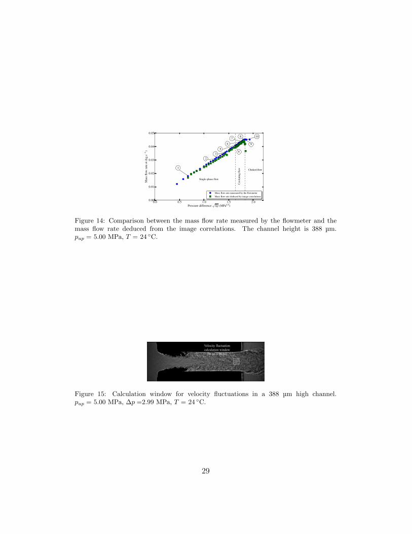
Figure 14: Comparison between the mass flow rate measured by the flowmeter and themass flow rate deduced from the image correlations. The channel height is 388 µm.pup = 5.00 MPa, T = 24 ◦C.

Velocity fluctuation

calculation window

(96 px x 96 px)

Figure 15: Calculation window for velocity fluctuations in a 388 µm high channel.pup = 5.00 MPa, ∆p =2.99 MPa, T = 24 ◦C.

29

Figure 16: Relative velocity fluctuations versus Reynolds number Re (a), Nurick cavitationnumber KN (b) and normalized length of vapor cavities lnorm (c). The channel height is388 µm. pup = 5.00 MPa, T = 24 ◦C.

Figure 17: Relative velocity fluctuations versus normalized length of vapor cavities lnormfor different channel heights. pup = 5.00 MPa, T = 24 ◦C.

30