variations in sedimentological properties in lake challa...
TRANSCRIPT

FACULTY OF SCIENCES
Master of Science in geology
Academic year 2015–2016
Master’s dissertation submitted in partial fulfillment of the requirements for the degree of Master in Science in Geology
Promotor: Dr. I. Meyer Tutor: Drs. M. Dumon Jury: Prof. Dr. T. Vandenbroucke, Prof. Dr. S. Bertrand
Variations in sedimentological properties in Lake Challa, East Africa: Understanding the
source to sink processes
Jonas Eloy

Picture cover sheet: View on Lake Challa (source: www.tanzania-experience.com).

ACKNOWLEDGEMENTS
The completion of this thesis would never have been possible without the help and support
of numerous people during the last few months. Therefore, I would like to thank all of them
personally on this page, as they have been very important.
First of all, I would like to thank my promotor Dr. Inka Meyer for giving me the opportunity
to investigate this inspiring topic. Her overall guidance, knowledge, dedicated time and
enthusiasm were very much appreciated and helped me a lot in finalizing this thesis. I really
enjoyed our collaboration and I wish her the best for the future.
A sincere thank you also goes to my tutor Drs. Mathijs Dumon for dedicating a lot of his time
in answering my questions and for guiding me through the theoretical part of the X-ray
diffraction analyses.
I also want to thank Veerle Vandenhende for helping and guiding me in the Laboratory of
Soil Science of the Geology and Soil Science Department. Always smiling, she gave me many
insights into the practical aspects of the X-ray diffraction method.
More gratitude also goes to Maarten Van Daele, Sébastien Bertrand, Carmen Juan
Valenzuela and Evelien Boes of the RCMG Department for explaining the various software
packages I worked with and for all sorts of small advice and contributions.
An enormous thank you must also be dedicated to all my friends and classmates during the
last five years. All those joyful moments were amazing and made my student life something
to cherish forever and to be never forgotten!
Last but not least, I want to thank my girlfriend Sara and my parents for their more than
endless motivating support and love throughout the thesis period and moreover during my
entire academic career. Without them, I would not stand where I am now!

TABLE OF CONTENTS
1 INTRODUCTION ......................................................................................................... 1
1.1 State-of-the-art and research objectives .................................................................... 1
1.2 Thesis outline ............................................................................................................... 3
2 STUDY AREA .............................................................................................................. 4
2.1 Geological setting ........................................................................................................ 4
2.2 Geographical setting .................................................................................................... 5
2.2.1 Sedimentology ...................................................................................................... 7
2.2.2 Hydrology ............................................................................................................. 7
2.3 Present day East African climate ................................................................................. 8
3 MATERIALS AND METHODS ..................................................................................... 10
3.1 Onshore samples ....................................................................................................... 10
3.1.1 Sample acquisition ............................................................................................. 10
3.1.2 Grain-size measurements ................................................................................... 10
3.1.3 Quantitative X-ray diffraction ............................................................................ 12
3.2 Short cores ................................................................................................................. 14
3.2.1 Sample acquisition ............................................................................................. 14
3.2.2 Core opening, core photography and macroscopic core description ................ 14
3.2.3 Multi-Sensor Core Logging ................................................................................. 15
3.2.4 Grain-size measurements ................................................................................... 15
3.3 Surface samples ......................................................................................................... 16
3.3.1 Sample acquisition ............................................................................................. 16
3.3.2 Grain-size measurements ................................................................................... 17
3.3.3 Quantitative X-ray diffraction ............................................................................ 17
4 RESULTS .................................................................................................................. 18
4.1 Onshore samples ....................................................................................................... 18
4.1.1 Grain-size measurements ................................................................................... 18
4.1.2 Quantitative X-ray diffraction ............................................................................ 24
4.2 Short cores ................................................................................................................. 29
4.2.1 Grain-size measurements ................................................................................... 29
4.2.2 Multi-Sensor Core Logging ................................................................................. 29

4.3 Surface samples ......................................................................................................... 32
4.3.1 Grain-size measurements ................................................................................... 32
4.3.2 Quantitative X-ray diffraction ............................................................................ 32
5 DISCUSSION ............................................................................................................ 34
5.1 Controls on sedimentological properties .................................................................. 34
5.1.1 Onshore grain-size distributions and their spatial variations ............................ 34
5.1.2 Short core grain-size distributions and inter-core comparison ......................... 37
5.1.3 Surface grain-size distributions and their spatial variations .............................. 38
5.2 Controls on mineralogical properties ........................................................................ 41
5.2.1 On- and offshore XRD patterns and their spatial variations .............................. 41
5.3 Terrestrial source areas and source-to-sink processes at Lake Challa ...................... 46
6 CONCLUSIONS ......................................................................................................... 47
7 REFERENCES ............................................................................................................ 49
8 APPENDICES ............................................................................................................ 54

Chapter 1 – Introduction
1
1 INTRODUCTION
1.1 State-of-the-art and research objectives
As the concept of climate change is becoming more and more important every year,
our society desires to understand past and recent climate changes in all its aspects.
According to Ruddiman (2008), there are plenty of ways to study climatic variations on Earth
as these are stored in various natural archives such as tree rings, ice cores, peat deposits,
coral reefs and on- and offshore sedimentary deposits. Regarding the investigation of the
latter archive, a plurality of research methods are available. Deposits of terrestrial material
in sedimentary basins can be used to reconstruct paleoclimatic and/or paleoenvironmental
conditions (Holz et al., 2007; Prins et al., 2000; Stuut et al., 2002). However, in order to be
able to validate paleo records, it is of uttermost importance to comprehend the modern
conditions and the evolution of terrigenous particles. Those calibrations are very useful in
defining Earth’s past, modern and future surface processes and in performing provenance
studies (Allen, 2008a; Visher, 1969). As such, one of the aspects scientists aim to understand,
are modern “source-to-sink” processes in various on- and offshore environments at different
latitudes.
The term “source-to-sink” comprises everything that is related to sediment dynamic
processes such as erosion, transport and deposition. These processes take place on various
spatial (and temporal) scales, for example from long-distance transport between continents
and ocean basins to meter-sized features (e.g. small gullies and ditches) (Allen, 2008b).
From the erosional point of view (i.e. the ‘source’), sedimentary geologists primarily aim to
answer questions as: ‘How are erosional processes affected by climatic factors? Can climate
changes be derived from long- and/or short-term evolutions of eroding surfaces?
What determines the exact location and timing of for example the erosion of a clastic
sedimentary particle?’ (Allen, 2008a). From the depositional point of view (i.e. the ‘sink’),
following questions are attempted to be answered: ‘Where is the clastic particle originating
from? Via which transport mechanism has a terrestrial particle been transported to its final
site of deposition (i.e. a lake, a river, an ocean basin)?’ (Allen, 2008a).
The origin of terrestrial sediment particles from several on-land sources can be linked to
physical (e.g. cold/arid conditions) and/or chemical (e.g. warm/wet conditions) weathering
of the initial bedrock. Whether physical or chemical (or both) weathering dominantly occurs,
depends on the latitude (i.e. tropics vs. poles) and the geological setting (i.e. mountains,
glaciers, deserts, fluvial plains). These weathering processes result in the erosion of the
bedrock and clastic particles are subsequently transported to their final site of deposition
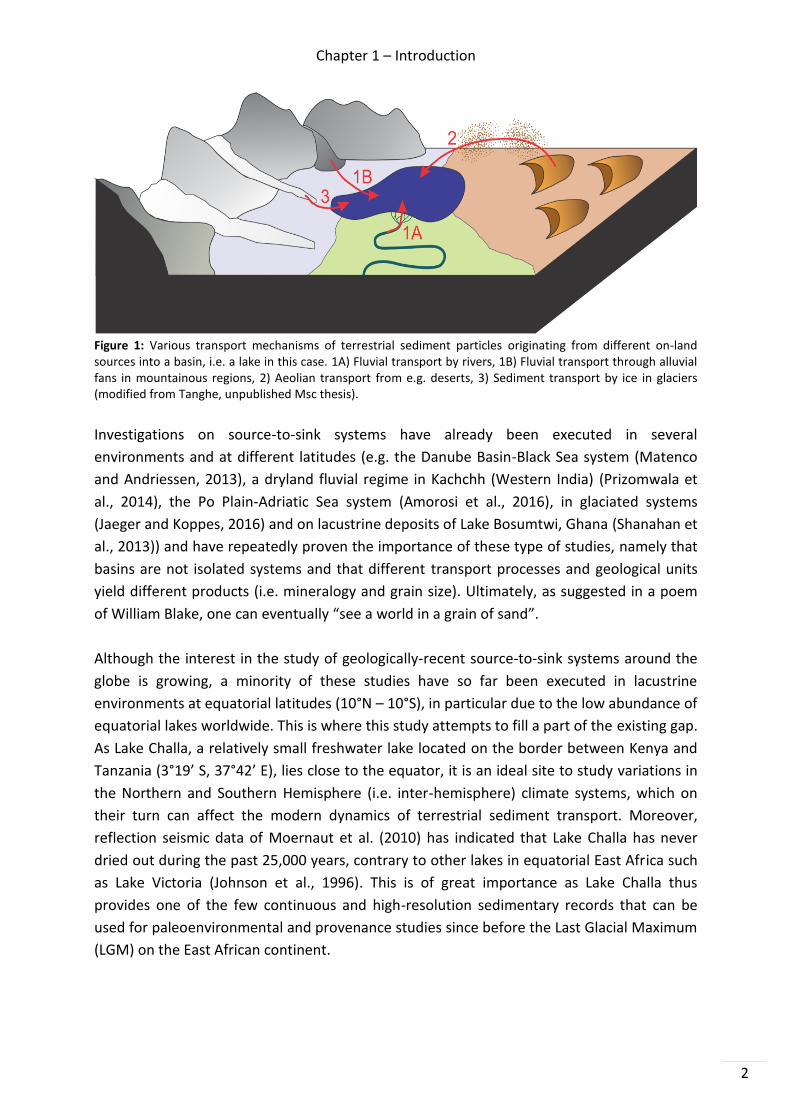
through various mechanisms (Figure 1). On a global scale, fluvial processes are responsible
for the largest quantities of terrestrial sediment transport, followed by aeolian processes in
more arid environments (Milliman and Syvitski, 1992).
Chapter 1 – Introduction
2
Figure 1: Various transport mechanisms of terrestrial sediment particles originating from different on-land sources into a basin, i.e. a lake in this case. 1A) Fluvial transport by rivers, 1B) Fluvial transport through alluvial fans in mountainous regions, 2) Aeolian transport from e.g. deserts, 3) Sediment transport by ice in glaciers (modified from Tanghe, unpublished Msc thesis).
Investigations on source-to-sink systems have already been executed in several
environments and at different latitudes (e.g. the Danube Basin-Black Sea system (Matenco
and Andriessen, 2013), a dryland fluvial regime in Kachchh (Western India) (Prizomwala et
al., 2014), the Po Plain-Adriatic Sea system (Amorosi et al., 2016), in glaciated systems
(Jaeger and Koppes, 2016) and on lacustrine deposits of Lake Bosumtwi, Ghana (Shanahan et
al., 2013)) and have repeatedly proven the importance of these type of studies, namely that
basins are not isolated systems and that different transport processes and geological units
yield different products (i.e. mineralogy and grain size). Ultimately, as suggested in a poem
of William Blake, one can eventually “see a world in a grain of sand”.
Although the interest in the study of geologically-recent source-to-sink systems around the
globe is growing, a minority of these studies have so far been executed in lacustrine
environments at equatorial latitudes (10°N – 10°S), in particular due to the low abundance of
equatorial lakes worldwide. This is where this study attempts to fill a part of the existing gap.
As Lake Challa, a relatively small freshwater lake located on the border between Kenya and
Tanzania (3°19’ S, 37°42’ E), lies close to the equator, it is an ideal site to study variations in
the Northern and Southern Hemisphere (i.e. inter-hemisphere) climate systems, which on
their turn can affect the modern dynamics of terrestrial sediment transport. Moreover,
reflection seismic data of Moernaut et al. (2010) has indicated that Lake Challa has never
dried out during the past 25,000 years, contrary to other lakes in equatorial East Africa such
as Lake Victoria (Johnson et al., 1996). This is of great importance as Lake Challa thus
provides one of the few continuous and high-resolution sedimentary records that can be
used for paleoenvironmental and provenance studies since before the Last Glacial Maximum
(LGM) on the East African continent.
Chapter 1 – Introduction
3
In order to identify and quantify modern dynamics of terrestrial sediment input into Lake
Challa, and to map out variations in sedimentological and mineralogical properties,
the clastic fraction of sediments from in- and outside Lake Challa are investigated in this
study. As such, a combination of samples from short cores and lacustrine surface sediment
samples as well as onshore samples from several locations around the lake and in the further
catchment will be analysed here with the aim in solving following research questions:
1. Through which transport mechanism(s) are onshore clastic particles transported towards
or into Lake Challa?
2. Can onshore clastic sediment characteristics be traced back in the lacustrine sediments?
3. Can distinct source areas be derived from the obtained results?
In order to answer these questions, detailed and high-resolution grain-size analysis together
with mineralogical analysis on the clastic sediments will be executed in this research,
with the purpose to understand the origin of terrigenous particles and to understand the
modern transport mechanisms at our study site. By investigating spatial variations in grain
size and mineralogy, information about distinct terrestrial source areas can be obtained.
To conclude, as James Hutton (1726 – 1797) once said ‘The present is the key to the past’,
it is essential to comprehend and quantify modern and geologically-recent (e.g. late-
Pleistocene-Holocene) transport mechanisms and source-to-sink systems in order to
understand ancient ones. By applying the results of the modern conditions on the downcore
record of Lake Challa, information about changes in sediment provenance and terrestrial
sediment input in the lake over time can be derived (Tanghe, unpublished Msc thesis).
1.2 Thesis outline
In the following chapter a concise summary of the geological and geographical setting as
well as the climatological background of the study area is given. Chapter 3 provides a
complete sequence of the used materials and methods and is divided according to the three
different types of sedimentary material: onshore samples, short cores and surface sediment
samples. Depending of the type of material, various sedimentological and geophysical
analysis techniques as well as the X-ray diffraction (XRD) technique will be explained.
Chapter 4 comprises a report of the obtained results of the three sediment groups.
In chapter 5 the results will be interpreted and discussed with the purpose to evidence links
between the three different sedimentary groups. Finally, the main conclusions of this
research are summarized in chapter 6. A few words will also be spent on future research,
since this study is rather exploring.

Chapter 2 – Study area
4
2 STUDY AREA
2.1 Geological setting
The geological history of East Africa is closely linked to the rise of the East-African Rift
System (EARS), also known as the Afro-Arabian Rift Valley, which represents an
approximately 4,500 km geographic trench that runs from the Afar Triple Junction in
northern Ethiopia through eastern Africa towards Mozambique in the south (Figure 2).
According to Baker et al. (1971), this is a classic example of an active continental rifting
system. The EARS consists of two branches, a western and an eastern one, which are still
tectonic and magmatic active. The more volcanically active eastern branch consists of
several segments, of which one is called the Kenya Rift. This segment (app. 600 km) extends
from Lake Turkana (northwest Kenya) to northern Tanzania (Figure 2) and started rifting in
the early Miocene around Lake Turkana in the north and subsequently further southwards
during the middle and late Miocene (Omenda, 2007). During the initial rifting phase up
doming and volcanism were the predominant processes, whereas during the early
Pleistocene a full graben system was formed (Omenda, 2007). The substrate consists of
erupted lava flows of basaltic and trachytic composition that were intercalated with tuffs.
Several large shield volcanoes of silicic composition were formed in the axis of the Kenya rift
during Quaternary times (Omenda, 2007). As such, the Mt. Kilimanjaro complex in northern
Tanzania started forming approximately 2.5 Ma ago and nowadays consists of three extinct
eruption centres: Shira, Mawenzi and Kibo. The last one went extinct about 150,000 years
ago. Due to numerous volcanic eruptions in the past, several craters were formed in the
proximity of this massive volcanic complex.
Lake Challa developed by filling up a caldera of Pleistocene age. As the lake lies on the
southeastern slope of Mt. Kilimanjaro, it is surrounded by igneous rocks (predominantly
trachy-basalts) of the tertiary Kilimanjaro complex (Bear, 1955). These basalts are covered by
“calcareous tuffaceous grits”, which is a calcite-cemented tuffaceous breccia that is probably
related to the formation of the Challa crater (Downie and Wilkinson, 1972). As observed by
Kristen (2010), these “calcareous tuffaceous grits” form the southeastern crater walls of
Lake Challa, whereas the rest of its crater rim mainly consists of trachy-basalts from the
Mt. Kilimanjaro complex. Finally, this volcanic complex is underlain by metamorphic rocks
(predominantly gneisses) that outcrop east and south of Lake Challa to the Indian Ocean
coast (Petters, 1991).

Chapter 2 – Study area
5
Figure 2: Left: simplified geological setting of the African continent. The East African Rift System has a Cenozoic age and is indicated with yellow. The red dot indicates the position of the Mt. Kilimanjaro complex (modified from Kampunzu and Popoff (1991)). Right: the Kenya-rift segment, which runs from Lake Turkana in the northwest of Kenya to Tanzania in the south (Omenda, 2007).
2.2 Geographical setting
Lake Challa is a small freshwater lake, located at 880 m altitude on the southeastern slope of
Mt. Kilimanjaro on the border between Kenya and Tanzania (3°19’ S, 37°42’ E) (Figure 3).
The lake has a surface area of approximately 4.5 km² and the maximum water depth varied
between 92 and 98 m during the period 1999 – 2010 (Wolff et al., 2014). The crater
catchment is rather small (1.38 km²) and consists entirely of steep crater walls, which reach
up to 170 m above the modern lake surface (Buckles et al., 2014). Additionally, during
periods of exceptionally heavy rainfall, the crater catchment can be marginally enlarged to
1.43 km² when a small creek of ca. 300 m located in the NW corner (Figure 3) of the lake is
temporarily active (Sinninghe Damsté et al., 2009; Verschuren et al., 2009).

Chapter 2 – Study area
6
Figure 3: Satellite image showing the geographic location of Lake Challa (3°19’ S, 37°42’ E) and its catchment on the southeastern slope of Mt. Kilimanjaro on the border between Kenya and Tanzania. The blue star in the figure below indicates the position of the 300 m small creek. Depth contours (Moernaut et al., 2010) are drawn at 10 m intervals to 90 m depth and at 94 m depth.

Chapter 2 – Study area
7
2.2.1 Sedimentology
In 2003 a detailed reflection seismic survey on the lake revealed an approximately 210 m
thick sedimentary infill of predominantly horizontal deposits, which is estimated to cover the
last ~250,000 years (Moernaut et al., 2010). In general, the sediments of Lake Challa are
nicely laminated, but the degree of lamination depends on the location within the lake.
Sediments in the centre of the lake are more laminated than sediments closer to shore.
The sediments have an autochthonous character since they are mainly composed of organic
matter, biogenic silica from diatoms and endogenic calcite. Nonetheless, fine-grained clastic
particles are also present in low, yet varying amounts. According to Kristen (2010), 10 to 40%
of the sediments consists of siliciclastic material. A closer study of the laminations indicates
the presence of light and dark laminae. According to Wolff et al. (2011), light laminae are
dominated by diatom frustules that are deposited during drier and windier months of
southern hemisphere winter (June – October). During this period a diatom bloom is initiated
by an increase in the amount of available nutrients due to upwelling processes.
During southern hemisphere summer (November – March), when the lake is biologically
productive, darker laminae are deposited. These are mainly composed of organic matter,
calcite crystals and terrestrial siliciclastic material. Sediment trap data of Wolff et al. (2011)
confirm that light-dark lamination couplets in Lake Challa reflect the seasonal delivery of
diatom-rich material during winter months and diatom-poor material during summer
months.
2.2.2 Hydrology
Lake Challa contains no surface in- or outflows, as water transport is limited by the presence
of steep crater walls, which confine the crater catchment. Instead, the water budget of
the lake is largely controlled by sub-surface in- and outflow, together with the local
precipitation (app. 600 mm/yr.) and evaporation (app. 1700 mm/yr.) balance (Payne, 1970).
The sub-surface inflow (app. 80% or 12.5 x 10⁶ m³) to Lake Challa derives from the
percolation of precipitation falling in the forests on the upper slopes of Mt. Kilimanjaro.
This inflow, mainly coming from the northwest, most likely also includes melt water of the
seasonal snow falling on the Mawenzi peak of Mt. Kilimanjaro (Figure 3) (Payne, 1970).
The remaining 20% of water input is due to local rainfall (app. 20% or 3 x 10⁶ m³).
On the other hand, approximately 55% (8.2 x 10⁶ m³) of the water output is due to
sub-surface outflow, which represents about 2.5% of the lake volume. The remaining 40% is
due to evaporation (Payne, 1970).

Chapter 2 – Study area
8
2.3 Present day East African climate
The local climate around Lake Challa is tropical and semi-arid, resulting in a dry scrub
savanna landscape with relatively open grasslands and communities of trees (Figure 4).
According to Schüler et al. (2012), the modern surrounding savanna vegetation includes
Acacia, Terminalia, Grewia and Combretum woodlands.
Figure 4: Two photographs showing the dry scrub savanna landscape around Lake Challa with open grasslands (left) and communities of trees (right) (Photos by Dan L. Perlman, http://ecolibrary.org).
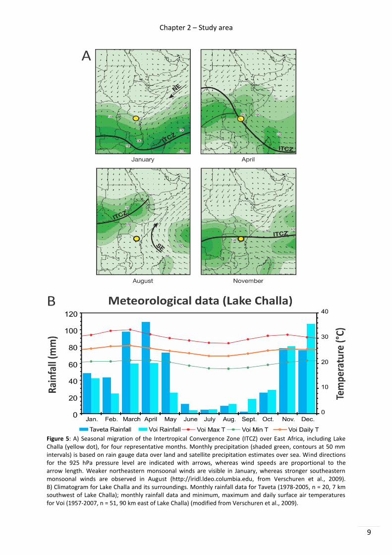
On a broader scale, the East African climate is largely controlled by the seasonal north-south
migration of the Intertropical Convergence Zone (ITCZ), which is associated with the
changing zenith position of the sun. As such, the ICTZ shifts northward during Northern
Hemisphere’s summer whereas the opposite movement occurs during Southern
Hemisphere’s summer (Figure 5A). This results in a bimodal rainfall pattern for tropical East
Africa, including Lake Challa, as Indian Ocean monsoonal winds bring precipitation to East
Africa twice per year (Figure 5B). The so called ‘long’ rains are produced by the southeasterly
monsoon from March to May/June and are responsible for the main amount of
precipitation, whereas the more variable ‘short’ rains, produced by the northeasterly
monsoon, are predominantly present from October to December (Figure 5A) (Nicholson,
1996). Both rainy seasons are separated by pronounced dry seasons in January – February
and mid-May through October (Figure 5B). The lowest mean daytime temperatures
(app. 26°C) occur during southern hemisphere winter (June – August), whereas the highest
temperatures (app. 30°C) occur during southern hemisphere summer (November – March).
In contrast to the temperature, seasonal wind speeds show the opposite pattern, with
weaker northeasterly trade winds prevailing from November to April and stronger
southeasterly winds from May to October when the ITCZ is displaced northward (Figure 5A)
(Kristen, 2010).
Chapter 2 – Study area
9
Figure 5: A) Seasonal migration of the Intertropical Convergence Zone (ITCZ) over East Africa, including Lake Challa (yellow dot), for four representative months. Monthly precipitation (shaded green, contours at 50 mm intervals) is based on rain gauge data over land and satellite precipitation estimates over sea. Wind directions for the 925 hPa pressure level are indicated with arrows, whereas wind speeds are proportional to the arrow length. Weaker northeastern monsoonal winds are visible in January, whereas stronger southeastern monsoonal winds are observed in August (http://iridl.ldeo.columbia.edu, from Verschuren et al., 2009). B) Climatogram for Lake Challa and its surroundings. Monthly rainfall data for Taveta (1978-2005, n = 20, 7 km southwest of Lake Challa); monthly rainfall data and minimum, maximum and daily surface air temperatures for Voi (1957-2007, n = 51, 90 km east of Lake Challa) (modified from Verschuren et al., 2009).

Chapter 3 – Materials and methods
10
3 MATERIALS AND METHODS
In order to gain a better understanding of the modern-day source to sink processes of
lacustrine deposits preserved in Lake Challa, three different sources of sedimentary material
were investigated: onshore samples, short cores and surface sediment samples. In this
chapter these three groups are introduced and the different methods that were applied on
each of them are explained.
3.1 Onshore samples
3.1.1 Sample acquisition
During two field campaigns in 2006 and 2010 multiple sediment samples originating from
several locations around Lake Challa and in its further catchment were retrieved.
Twenty-nine samples (called ‘Potsdam samples’ in the following) were obtained in
September 2006 by Kristen (2010), whereas the remaining thirty-seven samples (called
‘Utrecht samples’ in the following) were obtained in late January and early February 2010 by
the University of Utrecht (Buckles et al., 2014). Consequently, sixty-six onshore samples
were obtained and these are available to be investigated within this research (Appendix A).
As described by Kristen (2010), the ‘Potsdam samples’ consists of various surficial soil
samples that were randomly collected from grits and ditches, in addition to some volcanic
and metamorphic pebbles and rocks (e.g. basalts and gneisses). Three sampling locations
have been sampled twice, once for a pure rock sample and once for a corresponding soil
sample surrounding the rock (Appendix A). According to Buckles et al. (2014), the ‘Utrecht
samples’ purely consists of surficial soil samples that are further categorised as either red
(lateritic1) or grey (volcanic) types. The samples were retrieved from the lakeshore (L),
the crater rim (C), the hinterland (H), a small ravine in the NW corner of the lake (R) or from
combinations of these origins (Appendix A). They were randomly sampled from the 0 – 10
cm depth interval using a trowel, after removal of vegetation and litter (Buckles et al., 2014).
3.1.2 Grain-size measurements
As it is meaningless to determine grain-size distributions for rock samples or similar,
a sample selection has been done beforehand. As a consequence, ten samples out of
the twenty-nine ‘Potsdam samples’ were excluded for grain-size analysis as they represent
basalts, gneisses or other rocks (Appendix A). On the other hand, all thirty-seven ‘Utrecht
samples’ were retained for grain-size analysis as they consisted of fine-grained particles.
Grain-size measurements were executed for the remaining fifty-six samples (Figure 6) using
a Malvern Mastersizer 3000 at the University of Ghent (Laboratory for Sedimentology).
1 Rich in iron and aluminium, commonly originating in hot and wet tropical areas.

Chapter 3 – Materials and methods
11
Figure 6: Satellite images of Lake Challa (zoom) and its surrounding landscape, showing the spatial distribution of the three different sources of sedimentary material. The peculiar positioning of onshore samples LBK77, LBK78 and LBK81 within the lake instead of on the lakeshore is due to inaccurate GPS measurements. The yellow line represents the border between Kenya (E) and Tanzania (W) (source: Google Earth).
Prior to measuring, the terrigenous fraction was isolated first in three steps by successively
removing fine- and coarse-grained organic matter, carbonates and biogenic silica. Fine- and
coarse-grained organic matter was removed using loss-on-ignition (LOI; Heiri et al., 2001),
whereas carbonates and biogenic silica were dissolved by treating the samples (20 – 75 mg
in 10 ml DI water) with HCl (1 ml, 10%) and NaOH (1 ml, 2N) respectively.
These two chemical reactions were sped up by boiling the mixture for a few minutes on a
hot plate at 200°C. Finally, prior to analysis, 1 ml sodium hexametaphosphate ([NaPO3]6, 2%)
was added to the boiling mixture to ensure complete disintegration of particle aggregates.
Shortly after cooling, all fifty-six samples were successively inserted into the Malvern
Mastersizer 3000, using a Hydro Volume. The instrument measures grain-size distributions
based on the principle of laser diffraction. As a red and blue laser beam are propagating
through the dispersed sample in the sample measurement cell, they are being scattered due
to the interaction with a particle (Figure 7). As the red laser has a larger wavelength
(633 nm), it has difficulties in detecting the finer fraction. To solve this problem, a blue laser
(470 nm) is added for the more accurate detection of finer particles. Also, larger particles
scatter light at small diffraction angles, whereas smaller particles scatter light at large
diffraction angles. Diffracted rays are eventually detected by different detectors (Figure 7).

Chapter 3 – Materials and methods
12
Figure 7: The principle of laser diffraction, as occurring in the Malvern Mastersizer 3000. The red and blue laser pathways are shown, as well as the different detectors.
The angular variation in intensity of both scattered beams is measured and the scattering
pattern is afterwards converted to grain-size distributions ranging from 0.01 – 3500 µm.
Each sample was measured six to nine times, using the standard operating procedure (SOP2)
of S. Bertrand, in order to prevent random operator errors and to ensure reproducibility and
accuracy of the measurements. Finally, the Malvern Mastersizer 3000 data were exported
and subsequently used to calculate numerous descriptive grain-size distribution statistics
(e.g. mean, median, %sand, %silt,…) with the Excel macro-program GRADISTAT Version 8.0
(Blott and Pye, 2001), using the Folk and Ward graphical method (Folk and Ward, 1957).
3.1.3 Quantitative X-ray diffraction
The purpose of quantitative XRD (QXRD) analysis is to determine relative weight fractions for
every mineral phase present in a sample. In this study, twenty-six ‘Utrecht samples’ and
fourteen ‘Potsdam samples’ were carefully selected for quantitative analysis (Chapter 4,
Appendix E). The selection procedure was based on the sample location as well as on the
sample description. As such, distant samples and a few nearly coinciding samples were
excluded, based on their description. Similar to the grain-size measurements,
the terrigenous fraction was isolated in a first treatment phase by successively removing all
fine- and coarse grained organic matter and carbonates using the LOI procedure of Heiri et
al. (2001). In addition, four Potsdam samples were excluded from this procedure as they
consist of pure rocky material, which contains no organic matter or carbonates (Appendix E).
2 Measurement duration: 12 s, stirrer speed: 2500 RPM, ultrasonic sound: 10% of maximum power.
Chapter 3 – Materials and methods
13
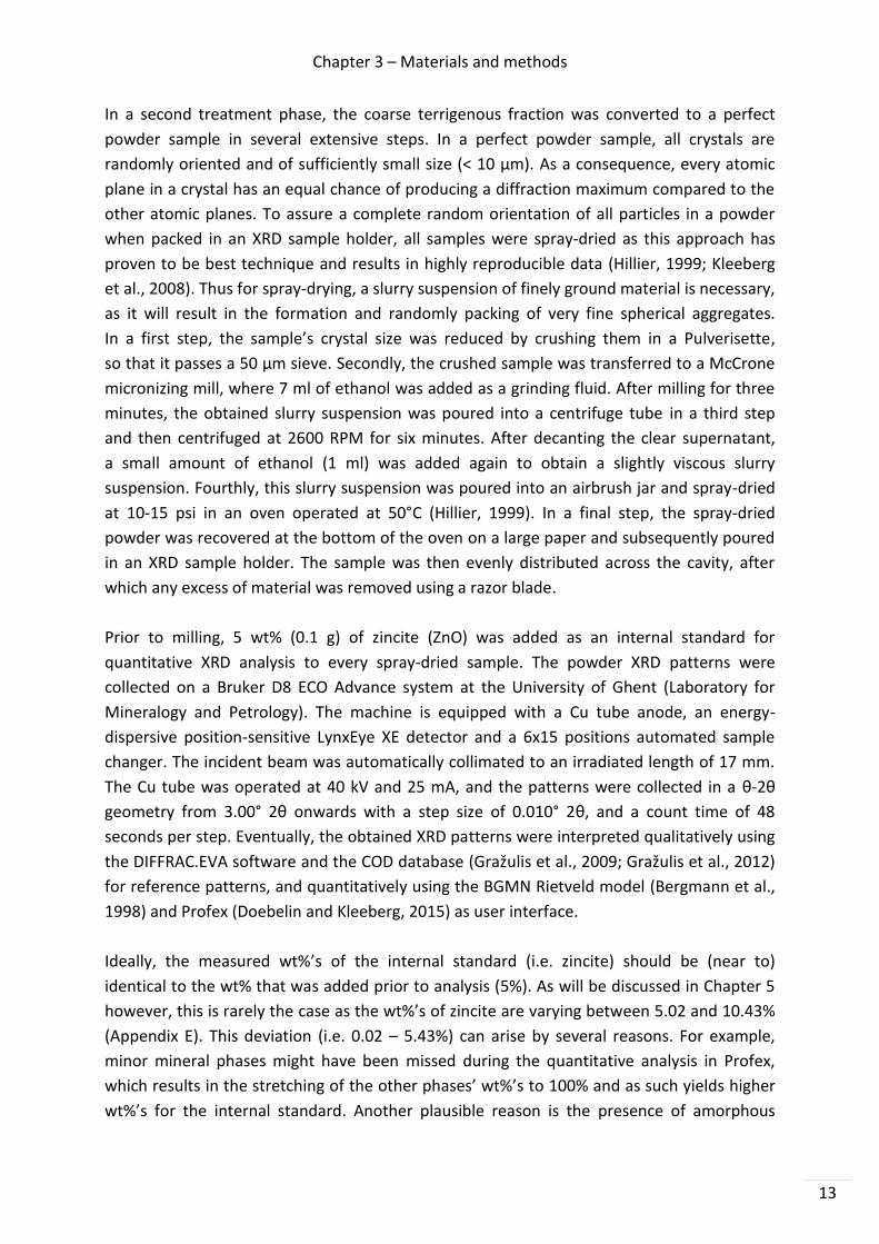
In a second treatment phase, the coarse terrigenous fraction was converted to a perfect
powder sample in several extensive steps. In a perfect powder sample, all crystals are
randomly oriented and of sufficiently small size (< 10 µm). As a consequence, every atomic
plane in a crystal has an equal chance of producing a diffraction maximum compared to the
other atomic planes. To assure a complete random orientation of all particles in a powder
when packed in an XRD sample holder, all samples were spray-dried as this approach has
proven to be best technique and results in highly reproducible data (Hillier, 1999; Kleeberg
et al., 2008). Thus for spray-drying, a slurry suspension of finely ground material is necessary,
as it will result in the formation and randomly packing of very fine spherical aggregates.
In a first step, the sample’s crystal size was reduced by crushing them in a Pulverisette,
so that it passes a 50 µm sieve. Secondly, the crushed sample was transferred to a McCrone
micronizing mill, where 7 ml of ethanol was added as a grinding fluid. After milling for three
minutes, the obtained slurry suspension was poured into a centrifuge tube in a third step
and then centrifuged at 2600 RPM for six minutes. After decanting the clear supernatant,
a small amount of ethanol (1 ml) was added again to obtain a slightly viscous slurry
suspension. Fourthly, this slurry suspension was poured into an airbrush jar and spray-dried
at 10-15 psi in an oven operated at 50°C (Hillier, 1999). In a final step, the spray-dried
powder was recovered at the bottom of the oven on a large paper and subsequently poured
in an XRD sample holder. The sample was then evenly distributed across the cavity, after
which any excess of material was removed using a razor blade.
Prior to milling, 5 wt% (0.1 g) of zincite (ZnO) was added as an internal standard for
quantitative XRD analysis to every spray-dried sample. The powder XRD patterns were
collected on a Bruker D8 ECO Advance system at the University of Ghent (Laboratory for
Mineralogy and Petrology). The machine is equipped with a Cu tube anode, an energy-
dispersive position-sensitive LynxEye XE detector and a 6x15 positions automated sample
changer. The incident beam was automatically collimated to an irradiated length of 17 mm.
The Cu tube was operated at 40 kV and 25 mA, and the patterns were collected in a θ-2θ
geometry from 3.00° 2θ onwards with a step size of 0.010° 2θ, and a count time of 48
seconds per step. Eventually, the obtained XRD patterns were interpreted qualitatively using
the DIFFRAC.EVA software and the COD database (Gražulis et al., 2009; Gražulis et al., 2012)
for reference patterns, and quantitatively using the BGMN Rietveld model (Bergmann et al.,
1998) and Profex (Doebelin and Kleeberg, 2015) as user interface.
Ideally, the measured wt%’s of the internal standard (i.e. zincite) should be (near to)
identical to the wt% that was added prior to analysis (5%). As will be discussed in Chapter 5
however, this is rarely the case as the wt%’s of zincite are varying between 5.02 and 10.43%
(Appendix E). This deviation (i.e. 0.02 – 5.43%) can arise by several reasons. For example,
minor mineral phases might have been missed during the quantitative analysis in Profex,
which results in the stretching of the other phases’ wt%’s to 100% and as such yields higher
wt%’s for the internal standard. Another plausible reason is the presence of amorphous

Chapter 3 – Materials and methods
14
material3, which scatters X-rays in many directions leading to one or more ranges with
increased background intensity instead of high intensity narrower peaks (Cullity, 1956).
These ‘humps’ in the background are fitted during the Rietveld refinement, but not
considered in the obtained weight percentage for the crystalline phases, which are always
scaled to 100%. This also results in wt%’s that are deviating from the ideal situation,
i.e. where no amorphous material is present. The amount of amorphous material can be
estimated by rescaling the obtained wt%’s using the known amount of the internal standard.
This rescaling is performed by multiplying each wt% by S/S’, where S is the known wt%
of zincite (5%) and S’ the obtained wt% of zincite (Appendix E, column 2). The amorphous
content is then calculated as follows: 100% * (1 - S/S’) (Appendix E, column 15).
Since the precision of quantitative X-ray analysis is not very high (deviations of at least a few
wt%’s are expected as repeatedly shown by international round-robin competitions (Madsen
et al., 2001; Omotoso et al., 2006; Ottner et al., 2000), the amorphous content must be
treated as a very rough estimation. The internal standard and amorphous material are not of
direct interest, so in order to ease comparison between the crystalline fraction of samples,
these were dropped from Appendix E and the remaining wt%’s are rescaled to 100%.
(Chapter 5, Table 1).
3.2 Short cores
3.2.1 Sample acquisition
To investigate lateral changes in sedimentological and geophysical properties of lacustrine
deposits of Lake Challa, five short cores of 19 to 36.2 cm length were retrieved with a
UWITEC gravity corer during a coring campaign in February 2005 by Kristen (2010).
They were taken along a horizontal transect from water depths ranging from 90 m near the
centre of the lake to 61 m near the shoreline of the northeastern crater rim (Appendix C.2,
Figure 6).
3.2.2 Core opening, core photography and macroscopic core description
At the University of Ghent (Geotek laboratory) the short cores were opened, photographed
and afterwards macroscopically described. Immediate imaging is necessary since rapid
oxidation of the sediment might occur, resulting in colour changes. The photographs were
taken by the Geotek GEOSCAN IV line scan camera, which is part of the Geotek Multi-Sensor
Core Logger (Figure 8). Afterwards, a virtual ruler was added onto the Geotek core images
using the Add Ruler v1.3 software. These precise depth-registered core images enable inter-
core comparison and are thus useful when describing the core.
3 Non-crystalline solids in which atoms and molecules are not organized in a definite lattice pattern e.g. glass.

Chapter 3 – Materials and methods
15
3.2.3 Multi-Sensor Core Logging
In order to obtain a high-resolution, downcore data set of the magnetic susceptibility (MS),
all short cores were scanned with a Geotek Multi-Sensor Core Logger (MSCL, Figure 8).
This geophysical property is of interest since changes in MS often correspond with changes
in mineralogy and sedimentary provenance (Loizeau et al., 2003; Maher, 2011).
The magnetic susceptibility was measured with a Bartington MS2E point sensor at a
precision of 10-5 SI. In addition, drift of the MS-sensor was monitored by executing
measurements in air after every 10th reading on the sediments. This drift value was then
automatically subtracted from the MS data by linear interpolation (Nowaczyk, 2001).
All magnetic susceptibility measurements were executed over discrete steps of 0.2 cm along
a central pathway on the core. Prior to analysis, the core halves were wrapped in a
protecting transparent foil since the MS-sensor was set to touch the sediment surface.
Figure 8: General set-up of a standard Multi-Sensor Core Logger (MSCL-S). In this study, only line-scan core imaging and magnetic susceptibility measurements were performed (Kempf, 2016).
3.2.4 Grain-size measurements
After carrying out the above-mentioned non-destructive methods, the sediment was
sampled in order to perform grain-size measurements with the Malvern Mastersizer 3000.
The sampling intervals were carefully selected based on a closer visual study of the core
images in Corel PHOTO-PAINT. The contrast was adjusted for every core image by executing
a histogram equalization, as this facilitated inter-core comparison. Additionally, MS data was

Chapter 3 – Materials and methods
16
superimposed on the core images to highlight zones with higher magnetic susceptibility
values, thus reflecting zones of interest (Chapter 4, Figure 13). Eventually, thirty-seven
sampling intervals from five short cores were selected for grain-size analysis (Figure 13).
As with the onshore samples, the terrigenous fraction was isolated. The samples (± 3 g in 10
ml DI water) were treated with H2O2 (8 ml, 35%) and HCl (3 ml, 10%) at 200°C to remove all
fine-grained organic matter and carbonates respectively. The removal of biogenic silica
(mostly diatoms), could not be established by the standard NaOH (1 ml, 2N) treatment, since
not all diatoms were dissolved. As suggested by Madella et al. (1998), the use of a non-toxic
heavy liquid is preferred for the extraction of diatoms. In this research sodium polytungstate
(Na6(H2W12O40)H2O) is used as heavy liquid with a varying density of 1.0 – 3.1 g/cm3.
The dense solution was diluted to 1.9 g/cm3, as this density was favourable for the
separation of the lighter diatoms (< 1.9 g/cm3) from the heavier clastic particles
(> 1.9 g/cm3).
Prior to the heavy liquid procedure, the fine fraction (< 4 µm) was separated first from the
coarse fraction (> 4 µm) by means of gravity sedimentation based on Stokes law4.
This was established by decanting the fine fraction four times with a time interval of 118
minutes between each decantation. Subsequently, this fraction was left to settle, whereas
the coarse fraction was used in the above-mentioned heavy liquid procedure. The separation
of clays is essential as a high concentration of these particles can obscure the mixture during
the heavy liquid process, leading to an insufficient extraction of diatoms (Madella et al.,
1998). At the end of the procedure, the clay fraction was again combined with the coarse
clastic fraction.
Finally, after adding 1 ml [NaPO3]6 (2%) to the samples, all thirty-seven samples were
successively inserted into the Malvern Mastersizer 3000 until the laser obscuration values
were in range (5 – 20%). Six measurements were performed for every sample, whereafter
the grain-size distributions were averaged and analysed with GRADISTAT Version 8.0
(Blott and Pye, 2001).
3.3 Surface samples
3.3.1 Sample acquisition
In addition to the above-mentioned Utrecht samples (section 3.1.1), nineteen profundal5
surface sediments were collected during the same field campaign in late January 2010
(Buckles et al., 2014). The sediments were recovered with intact sediment-water interfaces
4 v = g *D² * (density particle – density fluid) / (18 * viscosity), with g = 9.81 m/s² and D = particle size in µm.
5 Area of a lake that is located below the zone of effective light penetration, typically below the thermocline.
Chapter 3 – Materials and methods
17
from water depths ranging from 32.8 to 91.6 m using an UWITEC gravity corer (Appendix D,
Figure 6). In this research the 2-5 cm depth interval samples are investigated.
3.3.2 Grain-size measurements
As described before, the terrigenous fraction was isolated first by treating the samples
(± 2 g in 10 ml DI water) with H2O2 and HCl at 200°C. Due to a high concentration of bacteria
in the samples, a higher amount of H2O2 was added. The dissolution of bacteria is essential
since sediment particles were captivated within the bacteria frustules. As with the short core
samples, diatoms were removed by performing the heavy liquid procedure explained in
section 3.2.4. Afterwards, 1 ml [NaPO3]6 (2%) was added to the samples and subsequently
grain-size distributions were obtained using the Malvern Mastersizer 3000 and analysed with
GRADISTAT Version 8.0 (Blott and Pye, 2001).
3.3.3 Quantitative X-ray diffraction
All nineteen surface sediment samples were initially selected for quantitative XRD analysis.
Prior measurement, the terrigenous fraction was isolated first using LOI (Heiri et al., 2001).
Since 0.1 gram (5 wt%) of zincite (ZnO) is added as an internal standard to every sample, at
least two gram of sedimentary material is necessary for quantitative XRD analysis. After LOI
however, only one surface sample (11G) remained, since all the other samples had less than
two gram remaining. Consequently, sample 11G is the only surface sample suitable for
quantitative XRD analysis, as described in section 3.1.3.

Chapter 4 – Results
18
4 RESULTS
In this chapter the results of the grain-size measurements and the mineralogical analysis are
reported in detail for every sedimentary group consecutively. To describe grain-size
distributions, four major grain-size classes of the GRADISTATv8 program of Blott and Pye
(2001) will be used in the following chapters: clay (< 2 µm), silt (2 – 63 µm), sand (63 – 2000
µm) and gravel (2 – 64 mm). Throughout this chapter several figures are shown that will also
be used for the discussion. As such, references to these figures will be regularly used in
Chapter 5.
4.1 Onshore samples
4.1.1 Grain-size measurements
As mentioned in the previous chapter, fifty-six onshore samples (nineteen ‘Potsdam’
and thirty-seven ‘Utrecht’ samples) were suitable for carrying out grain-size analysis
(Appendix A, Figure 6). As it would be too extensive to present all fifty-six grain-size
distributions consecutively, a clustering approach is preferably chosen in this research with
the purpose to find along-shore differences in the grain-size distributions. As such, attempts
are made to group the samples based on their geographic location relative to Lake Challa,
together with a visual observation of every grain-size distribution. Although all fifty-six
samples are classified in various groups, they all have one thing in common, namely that
their grain-size distributions are polymodal and as consequence they are poorly sorted.
Yet, clear differences in the grain-size distributions can still be observed at different
locations around Lake Challa. The spatial distribution of the various onshore groups is shown
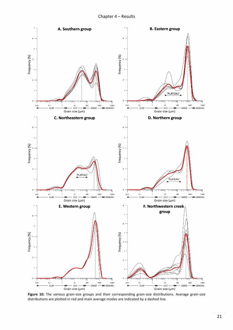
in Figure 9. The hereby associated grain-size distributions of every group are presented in
Figure 10A-J and consecutively described in the following paragraphs. Additionally, average
grain-size distributions have been plotted on top of the individual grain-size distributions of
each group separately. In Chapter 5 these groups will be further discussed.
The first group represents the sediments on the southern rim of the crater lake and
comprises the ‘Utrecht samples’ LBK76, LBK75, LBK74, LBK72, J12 and the nearby ‘Potsdam
samples’ 8 and 10 (Figure 9). All these samples are categorized as the ‘Southern group’ and
their corresponding grain-size distributions are plotted in Figure 10A. As indicated in the
figure, two average modes are present at app. 38 and 520 µm. As calculated by
GRADISTATv8, the majority of the sediments in every sample fall within the sand and silt
fraction (≥ 96.3%), with an average percentage of 97.8%. The average percentage of clay is
low, whereas gravel can be neglected (Appendix B).

Chapter 4 – Results
19
Figure 9: Satellite images of Lake Challa (zoom) and its surrounding landscape. The various proximal and distal onshore groups are indicated by different colours. The peculiar positioning of onshore samples LBK77, LBK78 and LBK81 within the lake instead of on the lakeshore is due to inaccurate GPS measurements. The 300 m small creek on the NW crater rim is indicated by a blue dashed line. The yellow line represents the border between Kenya (E) and Tanzania (W) (source: Google Earth).
The second group is representing the sediments on the eastern rim of the crater lake and
comprises the closely-spaced ‘Utrecht samples’ J01, J02, J03, J04 and samples J05 and J06
(Figure 9). As a consequence, these samples are categorized as the ‘Eastern group’ and the
individual grain-size distributions are shown in Figure 10B. Most of the distributions contain
a low frequency ‘plateau’ in the grain-size range of 10 – 200 µm, except for sample J03 which
shows a clear mode at about 20 µm. Secondly, all grain-size distributions show a high
frequency mode between app. 500 and 700 µm, with an average at app. 650 µm.
The average percentage of sand is higher compared to group 1 (66%, Appendix B). Similar to
group 1, the sediments in group 2 are dominated by sand and silt (≥ 92.6%), with an average
amount of 97.3%. Clay and gravel are again present in low and negligible amounts
respectively (Appendix B).
The third group is a small group that comprises the ‘Utrecht samples’ LBK62, LBK63 and
LBK77. As these are located on the crater rim in the northeastern corner of the lake
(Figure 9), they are categorized as the ‘Northeastern group’. Despite lying relatively close to
the ‘Utrecht samples’ J01, J02, J03, J04 of the previous group, their grain-size distributions
are different (Figure 10C). A ‘plateau’ is again present, this time with a slightly higher
frequency and in the grain-size range of 15 – 100 µm. Further, the average mode of the
higher frequency peak has decreased from 650 to app. 380 µm. Although the grain-size
distribution of sample LBK77 somewhat differs from the other two samples, it is classified in
this group as it lies on the lakeshore between sample LBK62 and LBK63. Therefore, LBK77 is
most likely influenced by both samples. Again, sand and silt are equally dominating the

Chapter 4 – Results
20
sediments (≥ 92.2%), with an average percentage of 94.8% (Appendix B). Since gravel is
completely absent, the remaining sediments are clays, with an average percentage of 5.21%.
The fourth group is also a small group comprising two ‘Utrecht samples’ LBK64 and LBK65
and ‘Potsdam sample’ 16, located on the northern rim of the crater lake (Figure 9).
The samples are categorized as the ‘Northern group’ and their grain-size distributions are
shown in Figure 10D. Samples LBK64 and LBK65 are similar to each other and different from
the previous group regarding the position of the high frequency mode around app. 580 µm.
No second mode is observed, however a ‘plateau’ is present in the grain-size range of
15 – 170 µm. Despite having a slightly different grain-size distribution, sample 16 is
categorized in this group according to its geographic location north of Lake Challa and
because of the presence of the mode around app. 580 µm. Although samples from the
northern group look similar to the ones of group 2, which have a higher frequency mode
between app. 500 and 700 µm (Figure 10B), they are categorized in a different group since
they are geographically separated up to 2 km. Appendix B shows the recurring dominance of
sand and silt (≥ 95.2%), with an average percentage of 96.3%. Finally, clay and gravel are
present in minor and negligible amounts respectively.
The fifth group only comprises two ‘Utrecht samples’ on the western rim of Lake Challa,
sample LBK70 and LBK71 (Figure 9). The grain-size distributions of these ‘Western group’
samples are shown in Figure 10E and are characterized by a high frequency mode between
app. 400 and 580 µm, with an average at app. 490 µm. Both samples are predominantly
sandy with an average percentage of 74.87%. The remaining sediment is mainly composed
of silt and a small amount of clays, with average values of respectively 23.14 and 1.99%.
In addition, gravel is completely absent (Appendix B).
The sixth group is a large group comprising the ‘Utrecht samples’ LBK68, LBK69, LBK79 and
LBK80 and the nearby located ‘Potsdam samples’ 15b, 19 and 32. All these samples are
located on the northwestern rim of the crater lake in the vicinity (< 200 m) of a 300 m small
creek (Figure 9) and are categorized as the ‘Northwestern creek group’. As illustrated in
Figure 10F, all grain-size distributions show at least two modes: an obvious first one with
varying frequency in the sand fraction between app. 350 and 580 µm (490 µm on average)
and another one in the clay fraction at app. 0,1 µm. Contrary to previous groups, a distinct
mode in the clay fraction is observed, which leads to higher percentages of clay in every
sample (Appendix B). Based on this characteristic, and because of the fact that all samples lie
in the vicinity of the small creek, they are categorized in the same group, although having
different grain-size distributions. Despite the higher percentages of clay, sand and silt remain
the main constituents of the sediment (≥ 66.9%, 80.3% on average), whereas gravel is
completely absent (Appendix B).
Chapter 4 – Results
21
Figure 10: The various grain-size groups and their corresponding grain-size distributions. Average grain-size distributions are plotted in red and main average modes are indicated by a dashed line.

Chapter 4 – Results
22
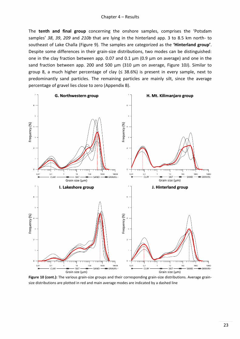
The seventh group is another large group representing the ‘Utrecht samples’ J07, J08, J09,
J10, J11 and LBK67 on the northwestern rim of the crater lake (Figure 9).
Contrary to the previous group, these samples do not lie in the vicinity of the 300 m small
creek and therefore the samples are categorized in a different group, namely the
‘Northwestern group’. The grain-size distributions are shown in Figure 10G. As with the
previous group, a clear mode is present at app. 0.1 µm, again resulting in higher percentages
of clay (Appendix B). On the other hand, a consistent mode in the sand fraction is missing as
the position and frequency of the modes are varying. Although remarkable variations are
visible in the silt and predominantly sand fraction, it makes sense to group these samples as
they were sampled along small streams on the NW crater rim during one field trip (Buckles
et al., 2014). Furthermore, Buckles et al. (2014) described these samples as being ‘Ravine-
Hinterland (RH)’ samples (Appendix A), so a similar origin can be assumed. Appendix B shows
the contribution of the different sedimentary constituents present in every sample.
As always, sand and silt are predominantly present (≥ 75.3%), with an average percentage of
82.3%.
The eighth group comprises the coupled ‘Utrecht samples’ LBK82 & LBK83 and LBK84 &
LBK85 and lies further northwest of Lake Challa (avg. 6.6 km), located closest to
Mt. Kilimanjaro of all onshore groups (Figure 9). As a result, the samples are categorized as
the ‘Mt. Kilimanjaro group’, despite lying a few km apart from each other. The grain-size
distributions shown in Figure 10H are all characterized by an obvious and almost consistent
mode at app. 0.075 µm. In comparison with the two previous groups, the frequency of this
mode is much higher, thus resulting in the highest percentage of clays of all onshore samples
(≤ 43.8%, Appendix B). The mode in the sand fraction is less consistent concerning its
position and frequency, yet it clearly indicates the dominance of sand over silt. The average
amount of gravel can be neglected (Appendix B).
The ninth group comprises the ‘Utrecht samples’ LBK81, LBK78 and the ‘Potsdam samples’
17/18, 20 and 21. As can be derived from Figure 9, these samples are located in different
geographic areas around Lake Challa. Therefore, geographical grouping is not the
appropriate approach. Nonetheless, the samples have two things in common: I) their
location on the lakeshore and II) the presence of a high frequency mode between app. 500
and 850 µm (670 µm on average, Figure 10I). As a consequence, they are being categorized
as the ‘Lakeshore group’. Despite the fact that these samples lie in the vicinity of some
samples of the above-mentioned groups, they are categorized differently due to some
differences in their grain-size distributions (Figure 10I). For example, existing modes have
changed in frequency and/or position or new smaller ones are observed. As with most of the
previous groups, the samples in this group are also mainly composed of sand and silt
(≥ 85.5%, 92.2% on average) with only a minor percentage of clays. The average percentage
of gravel is slightly higher, but still in practically negligible amounts (Appendix B).
Chapter 4 – Results
23
The tenth and final group concerning the onshore samples, comprises the ‘Potsdam
samples’ 38, 39, 209 and 210b that are lying in the hinterland app. 3 to 8.5 km north- to
southeast of Lake Challa (Figure 9). The samples are categorized as the ‘Hinterland group’.
Despite some differences in their grain-size distributions, two modes can be distinguished:
one in the clay fraction between app. 0.07 and 0.1 µm (0.9 µm on average) and one in the
sand fraction between app. 200 and 500 µm (310 µm on average, Figure 10J). Similar to
group 8, a much higher percentage of clay (≤ 38.6%) is present in every sample, next to
predominantly sand particles. The remaining particles are mainly silt, since the average
percentage of gravel lies close to zero (Appendix B).
Figure 10 (cont.): The various grain-size groups and their corresponding grain-size distributions. Average grain-
size distributions are plotted in red and main average modes are indicated by a dashed line

Chapter 4 – Results
24
The remaining ‘Utrecht samples’ LBK61, LBK66, LBK73 and ‘Potsdam samples’ 23, 24, 25,
27b, 40 and 41 are not categorized in any of the above-mentioned groups (Figure 9).
Firstly, the three ‘Utrecht samples’ are excluded because their grain-size distributions do not
match with the others in their respective geographic areas (i.e. group 5, 7 and 1).
The six ‘Potsdam samples’ are excluded for two reasons: firstly, the samples are lying further
away from each other and from Lake Challa (up to app. 64 km for sample 41), which makes
the grouping approach less appropriate. Secondly, all samples are mainly composed of
coarser material (sand and gravel) and in combination with the large offset to Lake Challa;
it is less likely that these particles leave a major trace behind on the lacustrine sediments,
since they need to be transported over greater distances by e.g. monsoonal winds.
To conclude, these samples will not be discussed anymore in Chapter 5.
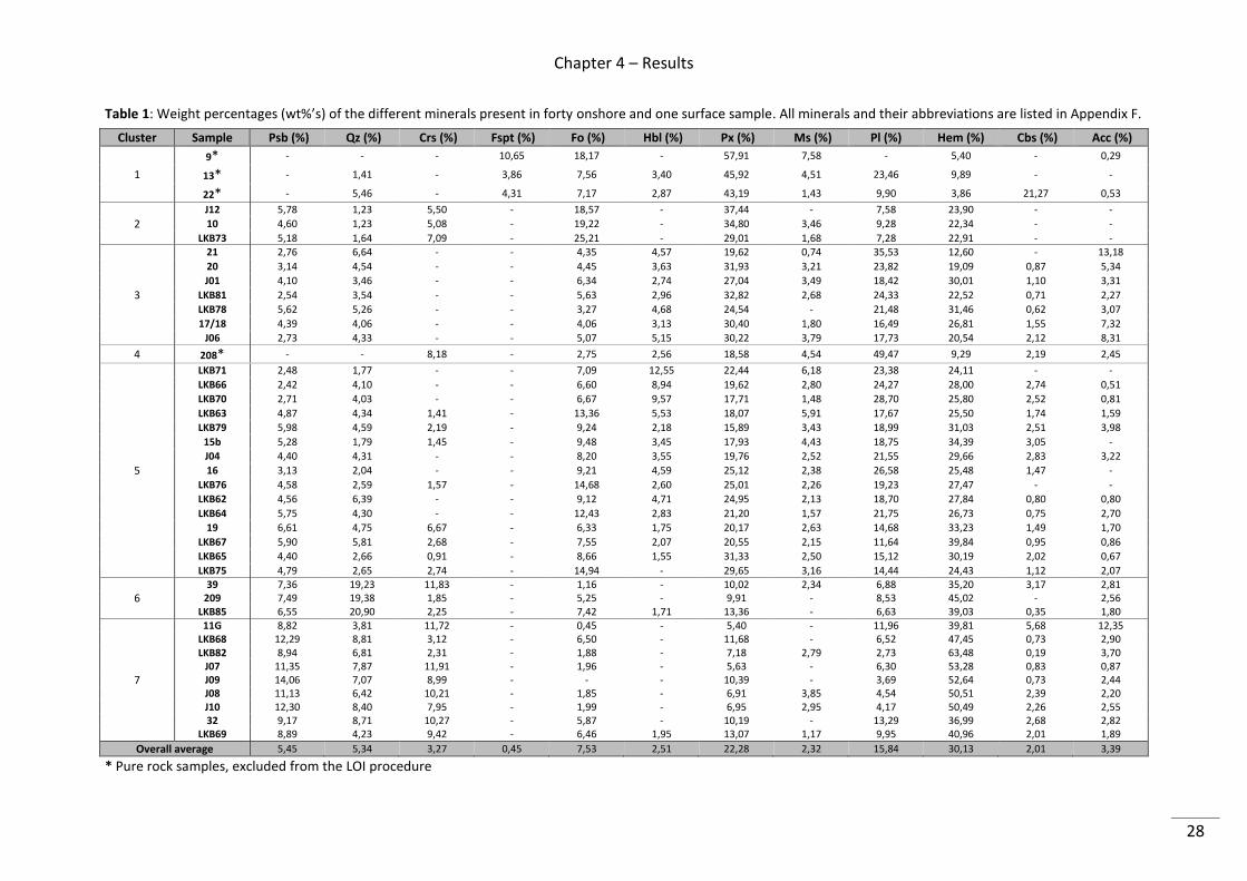
4.1.2 Quantitative X-ray diffraction
As mentioned in section 3.1.3, forty onshore samples (twenty-six ‘Utrecht’ and fourteen
‘Potsdam samples’) were carefully selected for quantitative X-ray diffraction analysis.
The obtained raw weight percentages (wt%’s) of the different minerals present in every
sample are shown in Appendix E, whereas the final, rescaled wt%’s of the crystalline
fraction (i.e. without amorphous content and internal standard) are shown in Table 1.
A brief explanation of every mineral/mineral group is given in Appendix F.
Similar to the grain-size measurements, it would be cumbersome to discuss the quantitative
XRD results of all forty onshore samples separately. A hierarchical cluster analysis was
instead performed on the weight percentages obtained via QXRD analysis (Table 1) and LOI
at 550°C and 950°C. For every mineral phase, the weight percentages were first normalized
by dividing each value by the standard deviation of the entire dataset. Afterwards,
the cluster analysis was performed using a Ward variance minimization algorithm
(Ward, 1963) as implemented in SciPy v0.16.1 (Jones et al., 2001). The final result of this
process is a XRD dendrogram (Figure 11). Based on the visual inspection of this dendrogram,
a cut-off distance (d) was chosen in order to select and define various clusters. In this case,
a cut-off distance of 7 was selected, resulting in a total of seven clusters (Figure 11).
The spatial distribution of these clusters is shown in Figure 12 and each cluster will be briefly
described in the paragraphs below.

Chapter 4 – Results
25
Figure 11: XRD dendrogram of forty onshore and one surface sample. The black lines represent the hierarchical clustering of the data. The red line indicates a cut-off distance of 7, resulting in seven clusters that are indicated by different colours below the red line.
Figure 12: Satellite images of Lake Challa (zoom), showing the spatial distribution of the different XRD clusters in colours matching those in the dendrogram (Figure 11). The peculiar positioning of onshore samples LBK78 and LBK81 within the lake instead of on the lakeshore is due to inaccurate GPS measurements. The 300 m small creek on the NW crater rim is indicated by a blue dashed line. The yellow line represents the border between Kenya (E) and Tanzania (W) (source: Google Earth).

Chapter 4 – Results
26
The first cluster comprises onshore samples 9, 13 and 22 (Figure 11, Table 1). These three
samples are three of the four rock samples that were excluded from the LOI procedure
(see section 3.1.3). Despite lying in different areas around Lake Challa (Figure 12),
the crystalline fraction is mainly characterized by a very high amount of pyroxenes.
Moreover, feldspathoids only occur in these three samples and the amount of hematite is
among the lowest of all samples. Pseudobrookite, cristobalite and carbonates are
completely absent. Remarkably, sample 22 contains a much higher percentage of carbonates
compared to the other two samples and in addition to all the other XRD samples (Table 1)
According to the BGMN Rietveld model of Bergmann et al. (1998), this is due to the presence
of variable calcite. As personally communicated by M. Dumon (Department of Geology,
Ghent University), this represents calcite with multiple Mg-for-Ca substitutions, although not
enough to be a dolomite. Because of the volcanic nature of the sediments around Lake
Challa, these substitutions are not remarkable. Since sample 22 is the only sample where
these high amounts of carbonates are observed, it should be treated with caution.
The second cluster consists of onshore samples J12, 10 and LBK73 (Figure 11, Table 1).
They are located on the southwestern crater rim of Lake Challa (Figure 12).
They predominantly consist of pyroxenes and hematite and have the highest amounts of
forsterite of all samples. Unheated sample 9 - although lying close to the other three
samples and being the sample with the 4th highest amount of forsterite - is not included in
this cluster.
The third cluster comprises onshore samples 21, 20, J01, LBK81, LBK78, 17/18 and J06
(Figure 11, Table 1). All of these samples are located on the lakeshore (Figure 12) and are
characterized by containing ‘higher’ amounts of accessory minerals compared to the other
samples. Yet, the percentages for these accessories are mostly low in comparison to the
predominantly present pyroxenes, plagioclases and hematite.
The fourth cluster only consists of onshore sample 208 (Figure 11, Table 1), being the fourth
rock sample that was excluded from the LOI procedure. Although located in the vicinity of
sample 22 (part of cluster 1, containing the other rock samples - Figure 12), sample 208
contains much more plagioclases than pyroxenes. Contrary to the other unheated samples
of the first cluster, cristobalite and carbonates are present whereas feldspathoids are
completely absent. Similarly, pseudobrookite is completely absent while the amount of
hematite is again among the lowest.
The fifth cluster is the largest cluster comprising onshore samples LBK71, LBK66, LBK70,
LBK63, LBK79, 15b, J04, 16, LBK76, LBK62, LBK64, 19, LBK67, LBK65 and LBK75 (Figure 11,
Table 1). All samples are scattered along the crater rim (Figure 12). As this cluster is centrally
positioned in the dendrogram, the wt%’s of the different mineral phases are differing the
least from the overall average wt%’s (Table 1). Yet, minor variations in the mineralogical

Chapter 4 – Results
27
composition of a few samples can be witnessed. For example, samples LBK63, LBK64, LBK75
and LBK76 contain higher amounts of forsterite than the overall average (Table 1), whereas
samples LBK70 and LBK71 have the highest amount of hornblende of all samples. Hematite,
pyroxenes and plagioclases are predominantly present, while the remaining mineral phases
are present in low, but varying amounts.
The sixth cluster comprises onshore samples 39, 209 and LBK85 (Figure 11, Table 1).
They are distally located east and west of Lake Challa (Figure 12) and are the only samples
containing a high amount of quartz. Compared to the previous clusters, pyroxenes and
plagioclases are present in lower amounts, whereas hematite is abundantly present.
The seventh and final cluster consists of onshore samples LBK68, LBK82, J07, J09, J08, J10,
32 and LBK69 (Figure 11, Table 1). They are located on the northwestern crater rim, except
sample LBK82 which lies further northwest (Figure 12), and are characterized by containing
the highest amounts of pseudobrookite and cristobalite. Moreover, the wt%’s of hematite
are also among the ten highest, except for sample 32. On the other hand, the wt%’s of
forsterite, pyroxenes and plagioclases are among the lowest of all samples. Despite lying in
the vicinity of some of the above-mentioned samples, samples 15b, 19 and LBK79 are not
included in this group. The only surface sample (11G) is also added to this group, as will be
explained in section 4.3.2.
Chapter 4 – Results
28
Table 1: Weight percentages (wt%’s) of the different minerals present in forty onshore and one surface sample. All minerals and their abbreviations are listed in Appendix F.
Cluster Sample Psb (%) Qz (%) Crs (%) Fspt (%) Fo (%) Hbl (%) Px (%) Ms (%) Pl (%) Hem (%) Cbs (%) Acc (%)
1
9* - - - 10,65 18,17 - 57,91 7,58 - 5,40 - 0,29
13* - 1,41 - 3,86 7,56 3,40 45,92 4,51 23,46 9,89 - -
22* - 5,46 - 4,31 7,17 2,87 43,19 1,43 9,90 3,86 21,27 0,53
2 J12 5,78 1,23 5,50 - 18,57 - 37,44 - 7,58 23,90 - -
10 4,60 1,23 5,08 - 19,22 - 34,80 3,46 9,28 22,34 - -
LKB73 5,18 1,64 7,09 - 25,21 - 29,01 1,68 7,28 22,91 - -
3
21 2,76 6,64 - - 4,35 4,57 19,62 0,74 35,53 12,60 - 13,18
20 3,14 4,54 - - 4,45 3,63 31,93 3,21 23,82 19,09 0,87 5,34
J01 4,10 3,46 - - 6,34 2,74 27,04 3,49 18,42 30,01 1,10 3,31
LKB81 2,54 3,54 - - 5,63 2,96 32,82 2,68 24,33 22,52 0,71 2,27
LKB78 5,62 5,26 - - 3,27 4,68 24,54 - 21,48 31,46 0,62 3,07
17/18 4,39 4,06 - - 4,06 3,13 30,40 1,80 16,49 26,81 1,55 7,32
J06 2,73 4,33 - - 5,07 5,15 30,22 3,79 17,73 20,54 2,12 8,31
4 208* - - 8,18 - 2,75 2,56 18,58 4,54 49,47 9,29 2,19 2,45
5
LKB71 2,48 1,77 - - 7,09 12,55 22,44 6,18 23,38 24,11 - -
LKB66 2,42 4,10 - - 6,60 8,94 19,62 2,80 24,27 28,00 2,74 0,51
LKB70 2,71 4,03 - - 6,67 9,57 17,71 1,48 28,70 25,80 2,52 0,81
LKB63 4,87 4,34 1,41 - 13,36 5,53 18,07 5,91 17,67 25,50 1,74 1,59
LKB79 5,98 4,59 2,19 - 9,24 2,18 15,89 3,43 18,99 31,03 2,51 3,98
15b 5,28 1,79 1,45 - 9,48 3,45 17,93 4,43 18,75 34,39 3,05 -
J04 4,40 4,31 - - 8,20 3,55 19,76 2,52 21,55 29,66 2,83 3,22
16 3,13 2,04 - - 9,21 4,59 25,12 2,38 26,58 25,48 1,47 -
LKB76 4,58 2,59 1,57 - 14,68 2,60 25,01 2,26 19,23 27,47 - -
LKB62 4,56 6,39 - - 9,12 4,71 24,95 2,13 18,70 27,84 0,80 0,80
LKB64 5,75 4,30 - - 12,43 2,83 21,20 1,57 21,75 26,73 0,75 2,70
19 6,61 4,75 6,67 - 6,33 1,75 20,17 2,63 14,68 33,23 1,49 1,70
LKB67 5,90 5,81 2,68 - 7,55 2,07 20,55 2,15 11,64 39,84 0,95 0,86
LKB65 4,40 2,66 0,91 - 8,66 1,55 31,33 2,50 15,12 30,19 2,02 0,67
LKB75 4,79 2,65 2,74 - 14,94 - 29,65 3,16 14,44 24,43 1,12 2,07
6 39 7,36 19,23 11,83 - 1,16 - 10,02 2,34 6,88 35,20 3,17 2,81
209 7,49 19,38 1,85 - 5,25 - 9,91 - 8,53 45,02 - 2,56 LKB85 6,55 20,90 2,25 - 7,42 1,71 13,36 - 6,63 39,03 0,35 1,80
7
11G 8,82 3,81 11,72 - 0,45 - 5,40 - 11,96 39,81 5,68 12,35 LKB68 12,29 8,81 3,12 - 6,50 - 11,68 - 6,52 47,45 0,73 2,90 LKB82 8,94 6,81 2,31 - 1,88 - 7,18 2,79 2,73 63,48 0,19 3,70
J07 11,35 7,87 11,91 - 1,96 - 5,63 - 6,30 53,28 0,83 0,87 J09 14,06 7,07 8,99 - - - 10,39 - 3,69 52,64 0,73 2,44 J08 11,13 6,42 10,21 - 1,85 - 6,91 3,85 4,54 50,51 2,39 2,20 J10 12,30 8,40 7,95 - 1,99 - 6,95 2,95 4,17 50,49 2,26 2,55 32 9,17 8,71 10,27 - 5,87 - 10,19 - 13,29 36,99 2,68 2,82
LKB69 8,89 4,23 9,42 - 6,46 1,95 13,07 1,17 9,95 40,96 2,01 1,89
Overall average 5,45 5,34 3,27 0,45 7,53 2,51 22,28 2,32 15,84 30,13 2,01 3,39
* Pure rock samples, excluded from the LOI procedure
Chapter 4 – Results
29
4.2 Short cores
4.2.1 Grain-size measurements
Figure 13 indicates thirty-seven sampling intervals, taken from five short cores in the
northeastern part of Lake Challa (Figure 6), that were selected for grain-size analysis.
The corresponding grain-size distributions of each interval are presented in Figure 14A-E for
every core separately. The average grain-size distribution of every core has been plotted on
top of it and all distributions, except the one of G12, clearly show the presence of a high and
broad frequency mode between app. 6 and 10 µm, accompanied by one and two low
frequency mode(s) in the clay and sand fraction respectively (Figure 14A-D). The frequency
of the main mode decreases from the centre (core G9) towards the shoreline (core G11),
whereas the frequencies of the smaller modes in the sand fraction increase along the same
transect (Figure 14A-D). As indicated in Appendix C.1, intervals with higher percentages of
sand or clay can be observed in every core. Appendix .2 shows the average amounts of clay,
silt, sand and gravel for every core. Sand and silt are clearly dominant and their percentages
show an opposite trend along the transect from core G12 to core G9, whereas those for clay
remain relatively low for every core (≤ 7.99%).
4.2.2 Multi-Sensor Core Logging
The patterns of magnetic susceptibility (MS) of the five short cores are shown in Figure 13.
A first remarkable observation regards the presence of two intervals with clearly elevated
MS values in every core except G9, which generally has very low MS values and only contains
one clear MS elevation at a core depth of approximately 35 – 36 cm. Secondly, elevated MS
intervals seem to occur in darker coloured zones (i.e. blueish intervals) at different core
depths, whereas lower MS values are occurring in brighter coloured zones (i.e. yellowish
intervals) that are located between the darker zones. These differences could possibly be
allocated to changes in sedimentological and/or mineralogical composition. A third and very
remarkable observation concerns the up to ten times higher MS values of core G12, which
could be related to its proximal location to the shore (Figure 13). The reason for the nearly
ten-fold drop in MS between core G12 and G11 (Figure 13) on the other hand,
is unexplainable so far since no quantitative XRD analyses were executed on the short cores.
Concerning the first two observations about the elevated MS values, the general relation
between MS and grain size, i.e. higher MS values for coarser-grained clastic sediments and
vice versa (Loizeau et al., 2003; Maher, 2011), was investigated. However, this relation
was fairly unsatisfying as elevated MS values also occurred in some finer-grained intervals
or even in intervals with neither more coarse or fine-grained material (Figure 13 vs.
Appendix C.1). As this downcore investigation also diverges from the main objectives of this
thesis, no further words on the magnetic susceptibility will be spent in the discussion.

Chapter 4 – Results
30
Figure 13: Short core images taken by the Geotek GEOSCAN IV line scan camera (Figure 8) and afterwards adjusted by performing a histogram equalization in Corel PHOTO-PAINT. Magnetic susceptibility data is superimposed on the core images (red curves) and the various sampling intervals for grain-size analysis (i.e. thirty-seven) are indicated by orange lines.

Chapter 4 – Results
31
Figure 14: A-E) Grain-size distributions of each interval within every short core (black curves). Average grain-size distributions are superimposed in red and the main average mode is indicated by a dashed line. F) Location of the short cores near the northeastern corner of Lake Challa. Depth contours (Moernaut et al., 2010) are drawn at 10 m intervals to 90 m depth and at 94 m depth.

Chapter 4 – Results
32
4.3 Surface samples
4.3.1 Grain-size measurements
As mentioned in Chapter 3, grain-size analyses were executed on nineteen profundal surface
sediments, retrieved from various depths and locations across Lake Challa (Figure 15A,
Appendix D). Contrary to the onshore samples, a clustering approach based on geographical
and/or sedimentological similarities is less appropriate here for two reasons: I) the coverage
of the lakes surface is unsatisfactory as the northern and southern part are not or barely
sampled (Figure 15A) and II) neither one grain-size distribution looks similar, as a wide range
of grain sizes is observed in every sample (Figure 15B). Yet, a broader high frequency mode
around 10 µm can again be seen in seventeen of the nineteen samples. As derived from
Appendix D, sand and silt are dominantly present in all the samples. The amount of clay
remains generally low (≤ 7.8%), except for four samples that are located in the northwestern
corner of the lake (Appendix D, Figure 15A). As always, gravel is not or barely found in these
surface samples.
4.3.2 Quantitative X-ray diffraction
As mentioned in section 3.3.3, unfortunately only one surface sample (11G) was selected for
quantitative XRD analysis. The obtained raw and rescaled weight percentages (wt%’s) of the
different minerals present in the sample are given in Appendix E and Table 1 respectively.
The sample lies in the NW corner of Lake Challa and is clustered with the onshore samples
on the northwestern crater rim (Figure 11, 7th cluster). It contains higher amounts of
pseudobrookite, cristobalite and hematite and lower amounts of forsterite, pyroxenes and
plagioclases. Additionally, higher amounts of carbonates and accessory minerals are also
present (Table 1).

Chapter 4 – Results
33
Figure 15: A) Location of nineteen surface sediment samples in Lake Challa. Depth contours (Moernaut et al., 2010) are drawn at 10 m intervals to 90 m depth and at 94 m depth. B) Corresponding nineteen grain-size distributions. Four distributions clearly show a higher frequency in the clay fraction below 0.4 µm.
Chapter 5 – Discussion
34
5 DISCUSSION
5.1 Controls on sedimentological properties
5.1.1 Onshore grain-size distributions and their spatial variations
In the previous chapter, fifty-six onshore samples were clustered into ten groups, each
representing a distinct area around Lake Challa or in its further catchment (Figure 9).
Although being spatially and sedimentologically different, the average grain-size
distributions of all groups are polymodal as they appear to consist of multiple sub
populations (Figure 10A-J). This polymodality is explained by the fact that clastic particles
often represent a mixture of material from different sources and/or from different transport
mechanisms (Holz et al., 2007). This explains the wider range of grain sizes in both the
‘Potsdam’ and the ‘Utrecht’ samples, as they were simply collected from the ground with a
shovel. Still, some remarkable variations were observed in various groups.
A clear mode in the clay fraction at app. 0.1 µm is present in the distal groups
‘Mt. Kilimanjaro’ and ‘Hinterland’ and in the proximal groups on the northwestern crater
rim, i.e. ‘Northwestern creek’ and ‘Northwestern’ (Figure 10F-H, 10J). The reason for the
existence of this clear mode is assumed to be due to fluvial processes. All four samples in the
‘Mt. Kilimanjaro group’ were sampled along two small stream beds (i.e. Lowari and
Lamsanga) that are most likely formed due to precipitation and melt water transport on the
southeastern slopes of the volcano (Buckles et al., 2014). During periods of rainfall, finer
eroded material is more easily picked up and transported via run-off processes and
afterwards deposited when the flow strength has decreased. Since the four samples lie
closest to Mt. Kilimanjaro (Figure 9), they are most affected by run-off processes,
consequently resulting in the highest percentage of clays of all onshore samples (43.8%,
Appendix B). A similar reasoning can be assumed for the samples in the ‘Northwestern
creek’ and ‘Northwestern’ group. The former group is affected by the nearby 300 m small
creek (Figure 9), while the latter group was sampled along several small streams (Buckles et
al., 2014). As mentioned in section 2.2, the creek is temporarily active during periods of
heavy rainfall. Moreover, the sampling area of both groups lies closest to Mt. Kilimanjaro
and is thus probably more affected, yet less than the ‘Mt. Kilimanjaro group’, by the
previously mentioned surficial transport (i.e. run-off) of sediment particles originating from
fluvial transport on the flanks of Mt. Kilimanjaro. Finally, the samples of the ‘Hinterland
group’ east of Lake Challa were sampled along a river bed (i.e. Lumi, Figure 16) and from
some ditches. Both sampling locations are again related to fluvial processes, which result in
the transport and subsequent deposition of very fine clay when currents become less strong.

Chapter 5 – Discussion
35
Figure 16 shows the comparison of a vegetation map of Sinninghe Damsté et al. (2011) with
a satellite image of Lake Challa and its surrounding landscape. The map shows that areas
west and northwest of the lake are mainly rainfed, which enhances fluvial transport.
The areas north- to southeast of Lake Challa on the other hand, are characterized by drier
open wood-, bush- and grasslands. These type of landscapes favor aeolian transport over
fluvial transport, yet the presence of the nearby Lumi river is suggested as a reason for the
presence of finer clay particles in the samples of the ‘Hinterland’ group (Appendix B,
Figure 16). River beds namely provide an ideal source of fine-grained material, although
more evidence is necessary here. Eventually, both observations east and west of Lake Challa
confirm the previous assumption that fluvial processes are responsible for the presence of
the app. 0.1 µm mode in the clay fraction in all four groups.
Figure 16: Comparison of a vegetation map of Lake Challa and its surrounding landscape (Sinninghe Damsté et al., 2011) with a satellite image of the same area (source: Google Earth) with the purpose to pinpoint various source areas and define different transport processes. The four onshore groups discussed in the paragraph above are indicated in colours matching those of Figure 9.
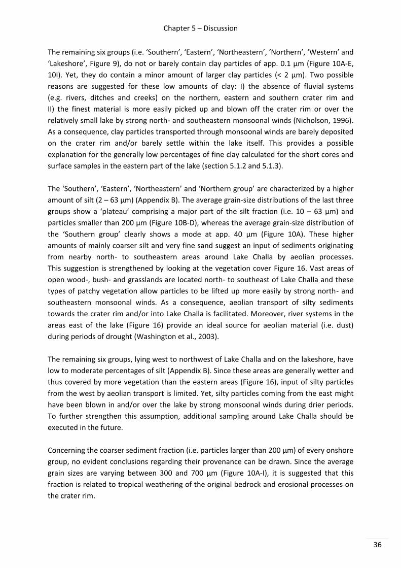
Chapter 5 – Discussion
36
The remaining six groups (i.e. ‘Southern’, ‘Eastern’, ‘Northeastern’, ‘Northern’, ‘Western’ and
‘Lakeshore’, Figure 9), do not or barely contain clay particles of app. 0.1 µm (Figure 10A-E,
10I). Yet, they do contain a minor amount of larger clay particles (< 2 µm). Two possible
reasons are suggested for these low amounts of clay: I) the absence of fluvial systems
(e.g. rivers, ditches and creeks) on the northern, eastern and southern crater rim and
II) the finest material is more easily picked up and blown off the crater rim or over the
relatively small lake by strong north- and southeastern monsoonal winds (Nicholson, 1996).
As a consequence, clay particles transported through monsoonal winds are barely deposited
on the crater rim and/or barely settle within the lake itself. This provides a possible
explanation for the generally low percentages of fine clay calculated for the short cores and
surface samples in the eastern part of the lake (section 5.1.2 and 5.1.3).
The ‘Southern’, ‘Eastern’, ‘Northeastern’ and ‘Northern group’ are characterized by a higher
amount of silt (2 – 63 µm) (Appendix B). The average grain-size distributions of the last three
groups show a ‘plateau’ comprising a major part of the silt fraction (i.e. 10 – 63 µm) and
particles smaller than 200 µm (Figure 10B-D), whereas the average grain-size distribution of
the ‘Southern group’ clearly shows a mode at app. 40 µm (Figure 10A). These higher
amounts of mainly coarser silt and very fine sand suggest an input of sediments originating
from nearby north- to southeastern areas around Lake Challa by aeolian processes.
This suggestion is strengthened by looking at the vegetation cover Figure 16. Vast areas of
open wood-, bush- and grasslands are located north- to southeast of Lake Challa and these
types of patchy vegetation allow particles to be lifted up more easily by strong north- and
southeastern monsoonal winds. As a consequence, aeolian transport of silty sediments
towards the crater rim and/or into Lake Challa is facilitated. Moreover, river systems in the
areas east of the lake (Figure 16) provide an ideal source for aeolian material (i.e. dust)
during periods of drought (Washington et al., 2003).
The remaining six groups, lying west to northwest of Lake Challa and on the lakeshore, have
low to moderate percentages of silt (Appendix B). Since these areas are generally wetter and
thus covered by more vegetation than the eastern areas (Figure 16), input of silty particles
from the west by aeolian transport is limited. Yet, silty particles coming from the east might
have been blown in and/or over the lake by strong monsoonal winds during drier periods.
To further strengthen this assumption, additional sampling around Lake Challa should be
executed in the future.
Concerning the coarser sediment fraction (i.e. particles larger than 200 µm) of every onshore
group, no evident conclusions regarding their provenance can be drawn. Since the average
grain sizes are varying between 300 and 700 µm (Figure 10A-I), it is suggested that this
fraction is related to tropical weathering of the original bedrock and erosional processes on
the crater rim.
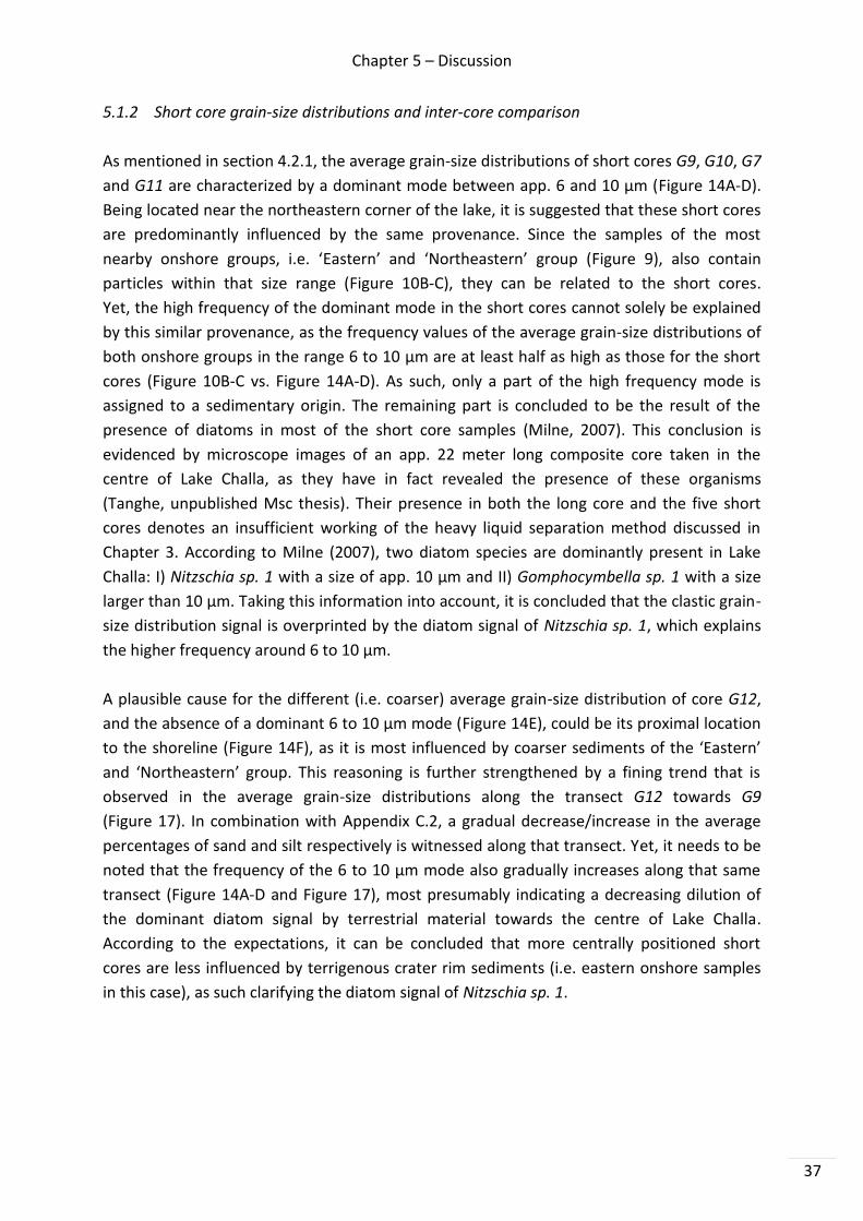
Chapter 5 – Discussion
37
5.1.2 Short core grain-size distributions and inter-core comparison
As mentioned in section 4.2.1, the average grain-size distributions of short cores G9, G10, G7
and G11 are characterized by a dominant mode between app. 6 and 10 µm (Figure 14A-D).
Being located near the northeastern corner of the lake, it is suggested that these short cores
are predominantly influenced by the same provenance. Since the samples of the most
nearby onshore groups, i.e. ‘Eastern’ and ‘Northeastern’ group (Figure 9), also contain
particles within that size range (Figure 10B-C), they can be related to the short cores.
Yet, the high frequency of the dominant mode in the short cores cannot solely be explained
by this similar provenance, as the frequency values of the average grain-size distributions of
both onshore groups in the range 6 to 10 µm are at least half as high as those for the short
cores (Figure 10B-C vs. Figure 14A-D). As such, only a part of the high frequency mode is
assigned to a sedimentary origin. The remaining part is concluded to be the result of the
presence of diatoms in most of the short core samples (Milne, 2007). This conclusion is
evidenced by microscope images of an app. 22 meter long composite core taken in the
centre of Lake Challa, as they have in fact revealed the presence of these organisms
(Tanghe, unpublished Msc thesis). Their presence in both the long core and the five short
cores denotes an insufficient working of the heavy liquid separation method discussed in
Chapter 3. According to Milne (2007), two diatom species are dominantly present in Lake
Challa: I) Nitzschia sp. 1 with a size of app. 10 µm and II) Gomphocymbella sp. 1 with a size
larger than 10 µm. Taking this information into account, it is concluded that the clastic grain-
size distribution signal is overprinted by the diatom signal of Nitzschia sp. 1, which explains
the higher frequency around 6 to 10 µm.
A plausible cause for the different (i.e. coarser) average grain-size distribution of core G12,
and the absence of a dominant 6 to 10 µm mode (Figure 14E), could be its proximal location
to the shoreline (Figure 14F), as it is most influenced by coarser sediments of the ‘Eastern’
and ‘Northeastern’ group. This reasoning is further strengthened by a fining trend that is
observed in the average grain-size distributions along the transect G12 towards G9
(Figure 17). In combination with Appendix C.2, a gradual decrease/increase in the average
percentages of sand and silt respectively is witnessed along that transect. Yet, it needs to be
noted that the frequency of the 6 to 10 µm mode also gradually increases along that same
transect (Figure 14A-D and Figure 17), most presumably indicating a decreasing dilution of
the dominant diatom signal by terrestrial material towards the centre of Lake Challa.
According to the expectations, it can be concluded that more centrally positioned short
cores are less influenced by terrigenous crater rim sediments (i.e. eastern onshore samples
in this case), as such clarifying the diatom signal of Nitzschia sp. 1.
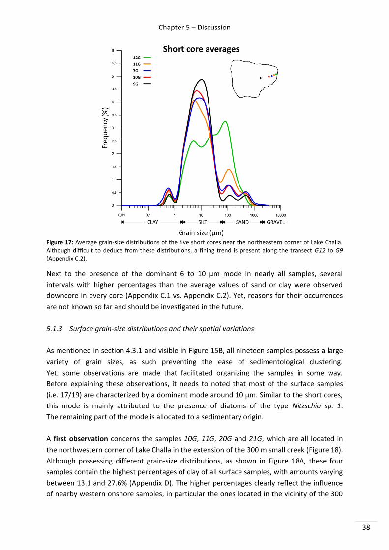
Chapter 5 – Discussion
38
Figure 17: Average grain-size distributions of the five short cores near the northeastern corner of Lake Challa. Although difficult to deduce from these distributions, a fining trend is present along the transect G12 to G9 (Appendix C.2).
Next to the presence of the dominant 6 to 10 µm mode in nearly all samples, several
intervals with higher percentages than the average values of sand or clay were observed
downcore in every core (Appendix C.1 vs. Appendix C.2). Yet, reasons for their occurrences
are not known so far and should be investigated in the future.
5.1.3 Surface grain-size distributions and their spatial variations
As mentioned in section 4.3.1 and visible in Figure 15B, all nineteen samples possess a large
variety of grain sizes, as such preventing the ease of sedimentological clustering.
Yet, some observations are made that facilitated organizing the samples in some way.
Before explaining these observations, it needs to noted that most of the surface samples
(i.e. 17/19) are characterized by a dominant mode around 10 µm. Similar to the short cores,
this mode is mainly attributed to the presence of diatoms of the type Nitzschia sp. 1.
The remaining part of the mode is allocated to a sedimentary origin.
A first observation concerns the samples 10G, 11G, 20G and 21G, which are all located in
the northwestern corner of Lake Challa in the extension of the 300 m small creek (Figure 18).
Although possessing different grain-size distributions, as shown in Figure 18A, these four
samples contain the highest percentages of clay of all surface samples, with amounts varying
between 13.1 and 27.6% (Appendix D). The higher percentages clearly reflect the influence
of nearby western onshore samples, in particular the ones located in the vicinity of the 300

Chapter 5 – Discussion
39
m creek (i.e. ‘Northwestern creek’ group, Figure 9). As derived from Appendix B and shown
in Figure 10F-G, higher amounts of clay were calculated for the ‘Northwestern creek’ and
‘Northwestern’ group. As the creek becomes active during periods of heavy rainfall,
fine sediments are transported and deposited into the lake. Since clays are much less
abundant in the rest of Lake Challa, it is suggested that samples in the northwestern corner
of the lake have an obvious western sedimentary source compared to the remaining surface
samples. This suggestion is further evidenced by quantitative X-ray diffraction data of
surface sample 11G, as explained in section 5.2.1.2.
A second observation concerns the curvy transect comprising sample 9G near the shoreline
(app. 280 m) over samples 8G, 7G and 6G towards sample 2G near the centre of the lake
(Figure 18). Their grain-size distributions show some similarities by possessing a small mode
in the clay fraction between app. 0.4 and 0.7 µm, a distinct mode at app. 6 µm and finally a
varying sand fraction with various smaller modes (Figure 18B). Sample 9G has the fifth
highest amount of clay (7.8%, Appendix D), which is in accordance to its more proximal
location to the 300 m creek as explained above. The other samples contain a lower,
but relatively stable clay content. According to the expectations, a fining trend is observed
along this transect. The percentage of sand is decreasing from sample 9G towards sample
2G, whereas the amount of silt is increasing to a maximum percentage of 90% in the latter
sample (Appendix D). Similar to the short cores in the eastern part of the lake, a decreasing
influence of mainly western onshore samples is concluded to be the reason for this
observation.
A third and final observation includes the surface samples 5G, 14G, 15G, 16G, 17G, 18G,
24G and 25G, which are located towards the eastern border of Lake Challa (Figure 18).
Their grain-size distributions are quite similar to those of the short cores by having a small
and consistent mode at app. 0.7 µm, a broader mode around 10 µm and finally a varying
sand fraction (Figure 18C). As with the short cores, the mode around 10 µm is mainly due to
diatoms of the type Nitzschia sp. 1 and partly due to sediment particles or the ‘Eastern’
group samples (cfr. section 5.1.2). In contrast to the short cores and the expectations,
no fining trend is observed along the arbitrarily-chosen transect from sample 14G over 15G,
25G and 17G towards 16G since the percentages of sand and silt are alternately
decreasing/increasing and increasing/decreasing (Appendix D). Because of their location,
a dominant influence of nearby eastern onshore samples (i.e. ‘Eastern’ group, Figure 9) is
expected. Yet, traces of the dominant mode in the sand fraction observed in the ‘Eastern’
group samples (app. 600 µm, Figure 10B), are barely observed in the grain-size distributions
of above-listed surface samples. Even the samples near the shoreline (i.e. 5G, 14G and 15G)
do not hold a high frequency mode in the sand fraction. It is therefore concluded that the
eastern crater rim induces much less fluvial transport or run-off into the lake, as no small
rivers, streams or creeks can be found there. Since the catchment east of Lake Challa is drier
(Figure 16), more aeolian transport in the eastern part of the lake is expected.

Chapter 5 – Discussion
40
Figure 18: A, B and C showing the grain-size distributions of the samples that are discussed in the first, second and third observation respectively. The locations of the samples in the three observations (A, B and C) are indicated in the lower right figure with red, yellow and purple respectively. The curvy transect of observation two is indicated with a yellow dashed line and the 300 m small creek on the NW crater rim by a blue star. Depth contours (Moernaut et al., 2010) are drawn at 10 m intervals to 90 m depth and at 94 m depth.

Chapter 5 – Discussion
41
5.2 Controls on mineralogical properties
5.2.1 On- and offshore XRD patterns and their spatial variations
In Chapter 4, forty onshore and one surface sample were separated in seven clusters
(Figure 11, Table 1) after the execution of a hierarchical cluster analysis in SciPy v0.16.1
(Jones et al., 2001). Similar to the various grain-size groups, every XRD cluster represents a
certain area on or near the crater rim of Lake Challa (Figure 12). Prior to interpreting these
different clusters, some critical thoughts must be given to the deviation of the obtained
wt%’s of zincite (Appendix E, column 2) from the percentage that was added prior to analysis
(5%) and to the remarkable presence of some mineral phases.
5.2.1.1 Influence of heating on XRD patterns
As mentioned in section 3.1.3, two plausible reasons were given for this deviation, which
varies between 0.02 and 5.43% (Appendix E). One concerned the occurrence of amorphous
material, which is present in varying amounts in all samples (Appendix E) and which leads to
unsatisfactory wt%’s. As amorphous material has previously been defined as ‘non-crystalline
solids in which atoms and molecules are not organized in a definite lattice pattern’,
past and/or recent heating processes are suggested as a plausible cause for its presence.
When soil samples in particular are being heated, either by volcanic processes in the past or
during the recently executed loss-on-ignition procedure at 550°C and 950°C, crystal lattices
disintegrate or deform, possibly resulting in the formation of X-ray amorphous material.
On the other hand, new mineral phases can be created after the deformation or
recrystallization of the initial mineral phases. For example accessory minerals akermanite
and mayenite, of which the occurrence around Lake Challa (Appendix E) was not expected,
are suggested to be mainly created during the LOI procedure (pers. Com. M. Dumon,
UGent). Moreover, both minerals can be created at high temperatures after the alteration of
siliceous limestones thus suggesting that perhaps calcite-bearing minerals were present
prior to LOI, but that they have disintegrated or recrystallized to akermanite and mayenite
upon heating (Appendix F). As mentioned in section 2.1, calcareous tuffaceous grits are
present at the surface around Lake Challa (Downie and Wilkinson, 1972) and these might act
as a calcite source.
The interpretation above is further strengthened by the relatively strong positive correlation
that is observed between the weight loss after LOI550, LOI950 and the occurrence of
akermanite and mayenite (Figure 19). This figure, also known as a heatmap, represents a
colour matrix of correlation coefficients between two parameters. Higher values (> 50%) are
observed in the lower right corner and evidence a relation between LOI and the occurrence

Chapter 5 – Discussion
42
of both accessory minerals. The occurrence of the carbonates magnesite, dolomite and lime
(CaO) can also be linked to LOI, but in lesser extent (Figure 19).
Figure 19: Heatmap representing the correlation coefficients between two parameters. Reddish colours indicate a positive correlation, whereas blueish colours a negative correlation. Striking is the strong positive correlation between both LOI procedures and the occurrence of the mineral phases ‘Akermanite’ and ‘Mayenite’.
Additional evidences for the influence of LOI on the XRD patterns could be derived from the
mineralogical composition of onshore samples 9, 13, 22 (Table 1, cluster 1) and 208 (Table 1,
cluster 4). These four samples consist of pure rocky material Appendix A) and they were
therefore excluded from the LOI procedure. Their mineralogical compositions revealed some
mutual similarities and remarkable differences with the other XRD samples that have
undergone the LOI procedure. For example, pseudobrookite is completely absent in all four
samples. So far, it is not fully understood if this is related to their rocky nature or if this
implies that it has been created in the other samples upon heating. Pseudobrookite can also
naturally occur within the Mt. Kilimanjaro volcanic complex (Anthony et al., 2003;
Appendix F). In contrast to pseudobrookite, feldspathoids only occur in three of the four
unheated samples (i.e. 9, 13 and 22, cluster 1), which thus suggests a link with LOI, although
Chapter 5 – Discussion
43
this cannot be proven so far. Further, the wt%’s of hematite of these four samples are the
lowest of all XRD samples. As hematite (Fe2O3) is formed upon heating of goethite (FeOOH)
at app. 300°C, it might have been created in the other soil samples during the LOI procedure.
Thought, caution must be paid as goethite is mainly formed through the weathering of iron-
rich minerals in laterite soils. As a result, the amount of goethite was probably higher already
for all the soil samples, logically resulting in higher amounts of clay-sized hematite after the
LOI procedure. The influence of LOI solely on the wt%’s of hematite can therefore not be
concluded. Finally, the wt%’s of the accessory minerals in samples 9, 13 and 22 are also
among the lowest of all XRD samples, thus strengthening the reasoning in the paragraph
above (i.e. LOI vs. accessories).
Due to above-mentioned examples, the influence of the LOI procedure on the onshore and
surface samples must therefore be considered during the interpretation of the various XRD
patterns. Yet, it needs to be noted that amorphous material or accessory minerals might
have been present in the samples even before LOI was performed as Lake Challa is
surrounded by sediments that possess a volcanic nature (Bear, 1955). The initial
mineralogical composition of every sample also played an important role of course, as every
mineral phase has a different degree of disintegration, deformation or recrystallization at
higher temperatures.
All these parameters must be kept in mind during the interpretation of the various clusters,
because the precision of quantitative X-ray analysis is not very high as proven by Madsen et
al. (2001), Omotoso et al (2006) and Ottner et al. (2000). The various mineralogical
compositions and clusters listed in Table 1 must therefore be treated as a rough estimation.
In the future, additional XRD analyses on unheated samples should be performed to approve
these roughly estimated compositions.
5.2.1.2 Spatial variations of XRD patterns
Although seven clusters have been defined during the hierarchical clustering analysis, it does
not imply that seven distinct source areas can be pinpointed around Lake Challa. First of all,
one must keep the volcanic nature of Lake Challa and its surrounding landscape in mind.
This obviously explains the abundance of pyroxenes, plagioclases and forsterite in nearly all
XRD samples (Table 1), as Lake Challa is surrounded by igneous rocks of the Mt. Kilimanjaro
complex (Bear, 1955) and underlain by metamorphic rocks (i.e. gneisses) (Petters, 1991).
Secondly, it must be mentioned that Lake Challa is a relatively small crater lake compared to
the size of the Tertiary Mt. Kilimanjaro complex. As a result, major differences in the spatial
variation of the various XRD patterns are not expected. Instead, minor variations were
observed between some clusters.
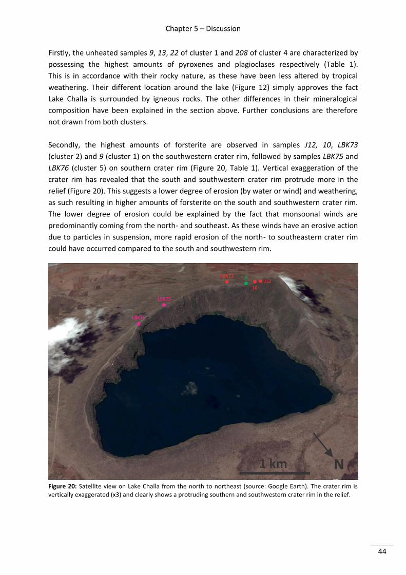
Chapter 5 – Discussion
44
Firstly, the unheated samples 9, 13, 22 of cluster 1 and 208 of cluster 4 are characterized by
possessing the highest amounts of pyroxenes and plagioclases respectively (Table 1).
This is in accordance with their rocky nature, as these have been less altered by tropical
weathering. Their different location around the lake (Figure 12) simply approves the fact
Lake Challa is surrounded by igneous rocks. The other differences in their mineralogical
composition have been explained in the section above. Further conclusions are therefore
not drawn from both clusters.
Secondly, the highest amounts of forsterite are observed in samples J12, 10, LBK73
(cluster 2) and 9 (cluster 1) on the southwestern crater rim, followed by samples LBK75 and
LBK76 (cluster 5) on southern crater rim (Figure 20, Table 1). Vertical exaggeration of the
crater rim has revealed that the south and southwestern crater rim protrude more in the
relief (Figure 20). This suggests a lower degree of erosion (by water or wind) and weathering,
as such resulting in higher amounts of forsterite on the south and southwestern crater rim.
The lower degree of erosion could be explained by the fact that monsoonal winds are
predominantly coming from the north- and southeast. As these winds have an erosive action
due to particles in suspension, more rapid erosion of the north- to southeastern crater rim
could have occurred compared to the south and southwestern rim.
Figure 20: Satellite view on Lake Challa from the north to northeast (source: Google Earth). The crater rim is vertically exaggerated (x3) and clearly shows a protruding southern and southwestern crater rim in the relief.
Chapter 5 – Discussion
45
Thirdly, the samples of the 7th cluster located on the northwestern crater rim
(Figure 12), all possess a different mineralogical composition compared to the other clusters
(Table 1). They are characterized by low amounts of forsterite, pyroxenes and plagioclases
and high amounts of hematite, pseudobrookite, quartz and cristobalite (Table 1).
The lower amounts of these volcanic minerals are suggested to be the result of enhanced
fluvial erosion and weathering by precipitation and melt water originating on the flanks of
Mt. Kilimanjaro in the northwest. As can be seen in Figure 20, the northwestern crater rim is
almost completely eroded. These observations correspond with the observations made for
the grain-size distributions in that area (i.e. ‘Northwestern’ and ‘Northwestern creek’ group,
section 5.1.1). As mentioned in section 4.3.2, the only surface sample 11G was also clustered
in cluster 7. Similar to the first observation made for the surface samples (section 5.1.3),
it evidences a distinct western sedimentary source as the mineralogical composition of
surface sample 11G largely corresponds with the northwestern onshore samples (Table 1).
Unfortunately, XRD patterns of other surface samples were not available to investigate other
possible source-to-sink processes into Lake Challa. Yet, using sample 11G as a clear example,
other source-to-sink processes might be detected in the remaining parts of Lake Challa if
additional sampling across the entire lake is executed in the future.
Finally, no decisive conclusions regarding provenance can be made based on the samples of
cluster 3, cluster 5 and cluster 6. Cluster 3 represents the samples taken on the lakeshore
(Figure 12) and their mineralogical compositions more or less correspond with the general
abundance of pyroxenes, plagioclases and hematite in the crater rim sediments (Table 1).
This corresponds with the expectations, namely erosion of crater rim material and
subsequent deposition on the lakeshore. Cluster 5 represents the largest cluster and
comprises samples that are scattered across the crater rim (Figure 12). Due to this spatial
scattering and because of the fact that their mineralogical compositions are differing the
least from the overall average, the data is insufficient to detect the exact provenance of the
various mineral phases that are present. Nonetheless, minor variations between some
samples within the cluster are observed, although these are of minor importance.
The distally located samples of cluster 6 eventually, possess similarities with the samples of
cluster 7, i.e. low amounts of forsterite, pyroxenes and plagioclases and higher amounts of
hematite, quartz and pseudobrookite, although the XRD signals are not easily traced back
into Lake Challa or its crater rim. Additional sampling in the future is therefore suggested.

Chapter 5 – Discussion
46
5.3 Terrestrial source areas and source-to-sink processes at Lake Challa
In this section, a brief summary of Chapter 5 is given with the eye on identifying distinct
terrestrial source areas and source-to-sink processes. One major finding of this study is that
the identification of distinct terrestrial source areas around Lake Challa is far from being
straight forward. Plenty of factors might have influenced the sedimentological and/or
mineralogical properties of the clastic sediments within and/or around Lake Challa.
For example, it must be reminded in the first place that the onshore samples were sampled
superficially (Appendix A), which complicates modern source-to-sink investigations and
provenance studies, since such samples often represent a mixture of signals originating from
various sources and/or transport mechanisms (i.e. run-off vs. aeolian) (Holz et al., 2007).
Moreover, minor variations in the spatial distribution of samples can lead to large
differences in grain-size distributions and/or X-ray diffraction patterns. This is evidenced by
the significant amount of defined onshore groups and XRD clusters, which was initially not
expected around the relatively small lake. Yet, differences between the groups and clusters
were in many cases not significantly high. Eventually, the most decisive observations in both
the grain-size distributions and the XRD patterns were made for the onshore samples on the
NW crater rim and for the associated surface sediments in the NW corner of the lake.
Both properties evidence the influence of a western sedimentary source and a fluvial
transport regime, compared to the rest of Lake Challa.
Besides difficulties on the source-side of the source-to-sink systems, difficulties were also
present on the sink-side. For example, the grain-size distributions of the lacustrine
sediments of Lake Challa were affected by the presence of diatoms, even though the heavy
liquid separation method was executed. This obstructed the search for a clear connection
between the clastic fraction of the lacustrine and crater rim sediments of Lake Challa.
Research into the mineralogical composition of the lacustrine sediments did not bring forth
much success either, as only one surface sample was available to evidence potential source-
to-sink relationships between the onshore samples and the lacustrine samples.

Chapter 6 – Conclusions
47
6 CONCLUSIONS
In this study an attempt was made to identify modern transport mechanisms of clastic
particles towards Lake Challa (Kenya/Tanzania) and to map out spatial variations in
sedimentological and mineralogical properties with the purpose to define distinct terrestrial
source areas. Therefore, high-resolution grain-size analyses were carried out on the clastic
fraction of three different sources of sedimentary material: onshore samples, short cores
and surface sediment samples. Mineralogical analyses were solely carried out on the
onshore samples and on one suitable surface sediment sample. Grain-size distributions were
obtained using the principle of laser diffraction in a Malvern Mastersizer 3000, after the
removal of abundant diatom frustules in a pre-treatment phase by applying a heavy liquid
separation method. Mineralogical analysis consisted of qualitative and quantitative X-ray
diffraction (XRD) analyses on a Bruker D8 Eco Advance system, after the prior removal of all
non-clastic fractions.
Given the significant amount of obtained grain-size distributions and X-ray diffraction
patterns for the onshore samples, a clustering approach was carried out for both properties
with the purpose to find along-shore differences in the grain-size distributions and in the
mineralogical compositions. Although not expected, ten different grain-size groups and
seven XRD clusters were defined around Lake Challa.
Despite the large amount of grain-size groups and XRD clusters, it does not imply that each
of them represents a distinct source area, since minor differences were observed in most
cases. Nonetheless, significant differences in grain-size distributions were observed
for two onshore groups on the northwestern crater rim (i.e. ‘Northwestern’ and
‘Northwestern creek’ group), one group further northwest closer to Mt. Kilimanjaro
(i.e. ‘Mt. Kilimanjaro’ group) and one proximal group north- to southeast of Lake Challa
(i.e. ‘Hinterland’ group). These four groups were characterized by significantly higher
amounts of clay, which are attributed to fluvial transport regimes (i.e. rivers, creeks, gullies)
west and east of Lake Challa. These regimes have originated due to precipitation and melt
water transport from the southeastern flanks of Mt. Kilimanjaro towards the southwest,
i.e. towards Lake Challa. Moreover, these fluvial regimes have resulted in a higher degree of
erosion and weathering of the northwestern crater rim, consequently also explaining the
significantly different mineralogical composition of the samples in that area (i.e. 7th cluster).
Contrary to the rest of the crater rim, this corner is characterized by low amounts of volcanic
minerals such as forsterite, pyroxenes and plagioclases. Moreover, a positive correlation was
observed between the grain-size distributions and the mineralogical compositions of the
northwestern crater rim sediments and the northwestern lacustrine surface sediments.
This is concluded to be a fluvial source-to-sink system with its origin located in western,
more vegetated and wetter areas.

Chapter 6 – Conclusions
48
The remaining onshore groups on the northern, eastern and southern crater rim on the
other hand, are barely affected by fluvial processes. Instead, these less vegetated and drier
areas are more affected by the erosive action of strong north- and southeastern monsoonal
winds (Nicholson, 1996), which prevent the deposition of very fine material on the rim and
subsequently within the lake. This is also evidenced by the generally low amounts of very
fine material observed in the eastern short cores and surface sediment samples. Aside the
low amounts of very fine material, higher amounts of silt were observed for both the eastern
lacustrine and onshore samples. This points out to an aeolian transport regime and an
eastern sedimentary source, although more evidence is necessary here.
As this study was rather exploratory, it also brought a few difficulties to light that offer
several opportunities regarding future research. For example, it has been pointed out that
most grain-size distributions of the lacustrine sediments (i.e. short cores and surface
sediment samples) of Lake Challa are strongly affected by the presence of diatom frustules
(Nitzschia sp. 1), even though they should have been removed by the heavy liquid separation
method. By improving this method in the future, diatoms will be completely removed, which
will facilitate the search for further possible source-to-sink systems around Lake Challa.
Furthermore, this study has repeatedly proven that the various mineralogical compositions
of heated samples around and within Lake Challa should be treated as a rough estimation,
as heating processes affected the mineralogical assemblages. Additional XRD analyses on
unheated samples should be executed in the future to further approve these roughly
estimated compositions. Finally, additional structured sampling within and around Lake
Challa should be carried out in the future with the purpose to obtain a satisfactory coverage
of both lacustrine and onshore deposits. This will aid in further investigations regarding
spatial variations in the sedimentological and mineralogical properties and in potential
source-to-sink relationships between the onshore and lacustrine samples of Lake Challa.
Chapter 7 – References
49
7 REFERENCES
Allen, P.A., 2008a, From landscapes into geological history: Nature, v. 451, no. 7176, p. 274–276.
Allen, P.A., 2008b, Time scales of tectonic landscapes and their sediment routing systems: Geological Society, London, Special Publications, v. 296, no. 1, p. 7–28.
Amorosi, A., Maselli, V., and Trincardi, F., 2016, Onshore to offshore anatomy of a late Quaternary source-to-sink system (Po Plain-Adriatic Sea, Italy): Earth-Science Reviews, v. 153, p. 212–237.
Anthony, J.W., Bideaux, R.A., Bladh, K.W., and Nichols, M.C., 2003, Eds., Handbook of Mineralogy, Mineralogical Society of America, Chantilly, VA 20151-1110, USA. http://www.handbookofmineralogy.org.
Baker, B.H., Williams, L.A.J., Miller, J.A., and Fitch, F.J., 1971, Sequence and geochronology of the Kenya rift volcanics: Tectonophysics, v. 11, no. 3, p. 191–215.
Bates, R.L., and Jackson, J.A., 1984, Dictionary of Geological Terms: Third Edition (Rocks, Minerals and Gemstones), American Geological Institute. p. 392.
Bear, L.M., 1955, Geology of the Taveta Area, Explanation of Degree Sheet 64 N.E. and 64 S.E. Report No. 32. (Geological Survey of Kenya, Ed.). Government Printer, Nairobi, p. 48.
Bergmann, J., Friedel, P., and Kleeberg, R., 1998, BGMN - a new fundamental parameter based Rietveld program for laboratory X-ray sources, its use in quantitative analysis and structure investigations: CPD Newsletter, Commission of Powder Diffraction, International Union of Crystallography, v. 20, p. 5–8.
Blott, S.J., and Pye, K., 2001, Gradistat: A grain size distribution and statistics package for the analysis of unconsolidated sediments: Earth Surface Processes and Landforms, v. 26, no. 11, p. 1237–1248.
Buckles, L.K., Weijers, J.W.H., Verschuren, D., and Sinninghe Damst, J.S., 2014, Sources of core and intact branched tetraether membrane lipids in the lacustrine environment: Anatomy of Lake Challa and its catchment, equatorial East Africa: Geochimica et Cosmochimica Acta, v. 140, p. 106–126.
Cullity, B.D., 1956, Elements of X-Ray Diffraction, 514 p. Addison-Wesley Publishing Company, Reading (Massachusetts, USA).
Doebelin, N., and Kleeberg, R., 2015, Profex : a graphical user interface for the Rietveld refinement program BGMN: Journal of Applied Crystallography, v. 48, no. 5, p. 1573–1580.
Downie, C., and Wilkinson, P., 1972, The Geology of Kilimanjaro: The Department of Geology, The University of Sheffield, Shefield, pp. 253, p. 373.
Chapter 7 – References
50
Folk, R.L., and Ward, W.C., 1957, Brazos river bar: A study in the significance of grain size parameters: Journal of Sedimentary Petrology, v. 27, no. 1, p. 3–26.
Gražulis, S., Chateigner, D., Downs, R.T., Yokochi, A.F.T., Quiros, M., Lutterotti, L., Manakova, E., Butkus, J., Moeck, P., and Le Bail, A., 2009, Crystallography Open Database - An open-access collection of crystal structures: Journal of Applied Crystallography, v. 42, no. 4, p. 726–729.
Gražulis, S., Daškevič, A., Merkys, A., Chateigner, D., Lutterotti, L., Quirós, M., Serebryanaya, N.R., Moeck, P., Downs, R.T., and Le Bail, A., 2012, Crystallography Open Database (COD): An open-access collection of crystal structures and platform for world-wide collaboration: Nucleic Acids Research, v. 40, no. D1, p. 420–427.
Heiri, O., Lotter, A.F., and Lemcke, G., 2001, Loss on ignition as a method for estimating organic and carbonate content in sediments: reproducibility and comparability of results: Paleolimnology, v. 25, p. 101–110.
Hillier, S., 1999, Use of an air brush to spray dry samples for X-ray powder diffraction: Clay Minerals, v. 34, no. 1, p. 127–135.
Holz, C., Stuut, J.B.W., Henrich, R., and Meggers, H., 2007, Variability in terrigenous sedimentation processes off northwest Africa and its relation to climate changes: Inferences from grain-size distributions of a Holocene marine sediment record: Sedimentary Geology, v. 202, no. 3, p. 499–508.
Jaeger, J.M., and Koppes, M.N., 2016, The role of the cryosphere in source-to-sink systems: Earth-Science Reviews, v. 153, p. 43–76.
Johnson, T.C., Scholz, C.A., Talbot, M.R., Kelts, K., Ricketts, R.D., Ngobi, G., Beuning, K., Ssemmanda, I., and McGill, J.W., 1996, Late Pleistocene desiccation of Lake Victoria and rapid evolution of cichlid fishes: Science, v. 273, no. 5278, p. 1091–1093.
Jones, E., Oliphant, E., and Peterson, P., 2001, SciPy: Open Source Scientific Tools for Python. http://www.scipy.org.
Kampunzu, A.B., and Popoff, M., 1991, Distribution of the main Phanerozoic African rifts and associated magmatism: introductory notes: Magmatism in extensional structural settings, p. 2–10.
Kempf, P., 2016, Tsunamis in south central Chili: evidence from coastal lakes: PhD Thesis; Ghent University (Ghent, Belgium).
Kleeberg, R., Monecke, T., and Hillier, S., 2008, Preferred orientation of mineral grains in sample mounts for quantitative XRD measurements: How random are powder samples? Clays and Clay Minerals, v. 56, no. 4, p. 404–415.
Kristen, I., 2010, Investigations on rainfall variability during the late Quaternary based on geochemical analyses of lake sediments from tropical and subtropical southern Africa: PhD Thesis; Deutsches GeoForschungsZentrum GFZ (Potsdam, Germany), 160 p.

Chapter 7 – References
51
Loizeau, J.-L., Rozé, S., Peytremann, C., Monna, F., and Dominik, J., 2003, Mapping sediment accumulation rate by using volume magnetic susceptibility core correlation in a contaminated bay (Lake Geneva , Switzerland): Eclogae Geologicae Helvetiae, v. 96, p. 73–79.
Madella, M., Powers-Jones, A.H., and Jones, M.K., 1998, A simple method of extraction of opal phytoliths from sediments using a non-toxic heavy liquid: Journal of Archaeological Science, v. 25, p. 801–803.
Madsen, I.C., Scarlett, N.V.Y., Cranswick, L.M.D., and Lwin, T., 2001, Outcomes of the International Union of Crystallography Commission on Powder Diffraction round robin on quantitative phase analysis: samples 1 a to 1 h: Journal of Applied Crystallography, v. 34, no. 4, p. 409–426.
Maher, B.A., 2011, The magnetic properties of Quaternary aeolian dusts and sediments, and their palaeoclimatic significance: Aeolian Research, v. 3, no. 2, p. 87–144.
Matenco, L., and Andriessen, P., 2013, Quantifying the mass transfer from mountain ranges to deposition in sedimentary basins: Source to sink studies in the Danube Basin-Black Sea system: Global and Planetary Change, v. 103, no. 1, p. 1–18.
Milliman, J.D., and Syvitski, J.P.M., 1992, Geomorphic/Tectonic Control of Sediment Discharge to the Ocean: The Importance of Small Mountainous Rivers: The Journal of Geology, v. 100, no. 5, p. 525–544.
Milne, I., 2007, Climate and environmental change inferred from diatom communities in Lake Challa (Kenya-Tanzania): Msc Thesis; Queen’s University (Ontario, Canada).
Moernaut, J., Verschuren, D., Charlet, F., Kristen, I., Fagot, M., and De Batist, M., 2010, The seismic-stratigraphic record of lake-level fluctuations in Lake Challa: Hydrological stability and change in equatorial East Africa over the last 140 kyr: Earth and Planetary Science Letters, v. 290, no. 1-2, p. 214–223.
Nicholson, S.E., 1996, A review of climate dynamics and climate variability in eastern Africa, in Johnson, T.C., Odada, E. (eds.), The Limnology, Climatology and Paleoclimatology of the East African Lakes. Gordon & Breach, p. 26–56.
Nowaczyk, N.R., 2001, Logging of magnetic susceptibility, in Tracking environmental change using lake sediments. (W.M. Last, and J.P. Smol, Eds.), p. 155-170 (Ch. 8), Kluwer Academic Publishers, Dordrecht.
Omenda, P.A., 2007, The geothermal activity of the past East African rift, in Presented at Short Course II on Surface Exploration for Geothermal Resources, organized by UNU-GTP and KenGen, at Lake Naivasha, Kenya, 2-17 November, 2007, p. 1–12.
Omotoso, O., McCarty, D.K., Hillier, S., and Kleeberg, R., 2006, Some successful approaches to quantitative mineral analysis as revealed by the 3rd reynolds cup contest: Clays and Clay Minerals, v. 54, no. 6, p. 748–760.
Chapter 7 – References
52
Ottner, F., Gier, S., Kuderna, M., and Schwaighofer, B., 2000, Results of an inter-laboratory comparison of methods for quantitative clay analysis: Applied Clay Science, v. 17, no. 5-6, p. 223–243.
Payne, B.R., 1970, Water balance of Lake Challa and its relation to groundwater from tritium and stable isotope data: Journal of Hydrology, v. 11, p. 47–58.
Petters, S.W., 1991, Regional Geology of Africa. Springer-Verlag, Berlin - Heidelberg, p. 722.
Prins, M.A., Postma, G., and Weltje, G.J., 2000, Controls on terrigenous sediment supply to the Arabian Sea during the late Quaternary: The Makran continental slope: Marine Geology, v. 169, no. 3-4, p. 351–371.
Prizomwala, S.P., Bhatt, N., and Basavaiah, N., 2014, Provenance discrimination and Source-to-Sink studies from a dryland fluvial regime: An example from Kachchh, western India: International Journal of Sediment Research, v. 29, no. 1, p. 99–109.
Ruddiman, W.F., 2008, Earth’s climate: Past and future (second edition). W.H. Freeman and Company, New York, 388 pp.
Schüler, L., Hemp, A., Zech, W., and Behling, H., 2012, Vegetation, climate and fire-dynamics in East Africa inferred from the Maundi crater pollen record from Mt Kilimanjaro during the last glacial-interglacial cycle: Quaternary Science Reviews, v. 39, p. 1–13.
Shanahan, T.M., McKay, N., Overpeck, J.T., Peck, J.A., Scholz, C., Heil, C.W., and King, J., 2013, Spatial and temporal variability in sedimentological and geochemical properties of sediments from an anoxic crater lake in West Africa: Implications for paleoenvironmental reconstructions: Palaeogeography, Palaeoclimatology, Palaeoecology, v. 374, p. 96–109.
Sinninghe Damsté, J.S., Ossebaar, J., Abbas, B., Schouten, S., and Verschuren, D., 2009, Fluxes and distribution of tetraether lipids in an equatorial African lake: Constraints on the application of the TEX86 palaeothermometer and BIT index in lacustrine settings: Geochimica et Cosmochimica Acta, v. 73, no. 14, p. 4232–4249.
Sinninghe Damsté, J.S., Verschuren, D., Ossebaar, J., Blokker, J., van Houten, R., van der Meer, M.T.J., Plessen, B., and Schouten, S., 2011, A 25,000-year record of climate-induced changes in lowland vegetation of eastern equatorial Africa revealed by the stable carbon-isotopic composition of fossil plant leaf waxes: Earth and Planetary Science Letters, v. 302, no. 1-2, p. 236–246.
Stuut, J.B.W., Prins, M.A., Schneider, R.R., Weltje, G.J., Fred Jansen, J.H., and Postma, G., 2002, A 300-kyr record of aridity and wind strength in southwestern Africa: Inferences from grain-size distributions of sediments on Walvis Ridge, SE Atlantic: Marine Geology, v. 180, no. 1-4, p. 221–233.
Verschuren, D., Sinninghe Damsté, J.S., Moernaut, J., Kristen, I., Blaauw, M., Fagot, M., and Haug, G.H., 2009, Half-precessional dynamics of monsoon rainfall near the East African Equator.: Nature, v. 462, no. 7273, p. 637–641.
Chapter 7 – References
53
Visher, G.S., 1969, Grain Size Distributions and Depositional Processes: Journal of Sedimentary Petrology, v. 39, no. 3, p. 1074–1106.
Ward, J.H., 1963, Hierarchical grouping to optimize an objective function: Journal of the American Statistical Association, v. 58, no. 301, p. 236–244.
Washington, R., Todd, M., Middleton, N.J., Andrew, S., Washington, R., Todd, M., Middleton, N.J., Washington, R., Todd, M., Middleton, N.J., and Goudie, A.S., 2003, Dust-Storm source areas determined by the total ozone monitoring spectrometer and surface observations: Annals of the Association of American Geographers, v. 93, no. 2, p. 297–313.
Wolff, C., Haug, G.H., Timmermann, A., Sinninghe Damsté, J.S., Brauer, A., Sigman, D.M., Cane, M.A., and Verschuren, D., 2011, Reduced interannual rainfall variability in East Africa during the last ice age: Science, v. 333, no. 6043, p. 743–747.
Wolff, C., Kristen-Jenny, I., Schettler, G., Plessen, B., Meyer, H., Dulski, P., Naumann, R., Brauer, A., Verschuren, D., and Haug, G.H., 2014, Modern seasonality in Lake Challa (Kenya/Tanzania) and its sedimentary documentation in recent lake sediments: Limnology and Oceanography, v. 59, no. 5, p. 1621–1636.

Chapter 8 – Appendices
54
8 APPENDICES
Appendix A: List of sixty-six onshore samples. Left: twenty-nine ‘Potsdam’ samples of Kristen (2010). Right: thirty-seven ‘Utrecht’ samples of Buckles et al. (2014), L: lakeshore, C: crater rim H: hinterland, R: ravine in the NW corner of the lake, CL; RH; RCH; RC and LR: combinations of different origins.
POTSDAM UTRECHT
Sample Type Lat (S) Lon (E) Sample Colour Depth (cm) Origin Lat (S) Lon (E)
208 rock* -3,314111 37,717200 J01 grey 0-3 L -3,314229 37,712415
209 soil -3,313944 37,733600 J02 grey 3-10 CL -3,314537 37,712567
210a rock* -3,371222 37,733600 J03 grey 0-6 CL -3,314465 37,712298
210b soil -3,371222 37,733600 J04 grey 0-4 C -3,313968 37,712946
8 soil -3,327479 37,702439 J05 grey 5-10 L -3,320329 37,707763
9 rock* -3,325397 37,687724 J06 grey NA CL -3,321801 37,705817
10 soil -3,324748 37,687204 J07 red 0-10 RH -3,306303 37,689279
11 rock/soil* -3,324539 37,686920 J08 red 0-10 RCH -3,304836 37,687580
13 rock/soil* -3,316342 37,686179 J09 red 0-10 RH -3,303604 37,686547
14 rock/soil* -3,315275 37,686399 J10 red NA RH -3,304635 37,686185
15a rock* -3,307834 37,687891 J11 red NA RH -3,305851 37,689234
15b soil -3,307834 37,687891 J12 red NA C -3,324362 37,686996
16 soil -3,307250 37,695063 LKB61 grey 0-4 L -3,318007 37,689011
17/18 soil -3,310556 37,709722 LKB62 grey 0-7 C -3,311480 37,712319
19 soil -3,309041 37,688550 LKB63 grey 0-6 C -3,309750 37,710063
20 soil -3,326685 37,695352 LKB64 grey 0-6 C -3,308768 37,706419
21 soil -3,324614 37,703077 LKB65 grey 0-6 C -3,308688 37,700453
22 rock* -3,314449 37,716681 LKB66 grey 0-6 C -3,307248 37,692625
23 soil -3,390253 37,730023 LKB67 red 0-6 C -3,306794 37,691006
24 soil -3,391841 37,777466 LKB68 red 0-6 RH -3,307874 37,686775
25a rock* -3,424081 37,638929 LKB69 red 0-8 RC -3,308418 37,687674
25b soil -3,424081 37,638929 LKB70 red 0-6 C -3,314746 37,685866
26 rock* -3,425503 37,647180 LKB71 grey 0-6 C -3,319722 37,686309
27 soil -3,424071 37,645587 LKB72 grey 0-6 C -3,324634 37,687032
32 soil -3,309723 37,686523 LKB73 grey/red 0-6 C -3,327911 37,689313
38 soil -3,254920 37,744909 LKB74 grey 0-6 C -3,328506 37,694757
39 soil -3,291344 37,736331 LKB75 grey 0-6 C -3,328348 37,698447
40 soil -3,394899 37,829334 LKB76 grey 0-6 C -3,327250 37,702463
41 soil -3,509794 38,258455 LKB77 litter 0-5 L -3,311333 37,710799
* Excluded for grain-size analysis LKB78 grey 3-3.5 L -3,310153 37,707668
LKB79 red 0-6 LR -3,308898 37,688681
LKB80 red 0-6 LR -3,308898 37,688681
LKB81 grey 0-6 L -3,308930 37,698635
LKB82 red 0-8 H -3,266870 37,636282
LKB83 red 0-7 H -3,266870 37,636282
LKB84 red 0-8 H -3,295946 37,634632
LKB85 red 0-7 H -3,295946 37,634632

Chapter 8 – Appendices
55
Appendix B: Grain-size results of ten defined onshore groups around Lake Challa.
Group Sample Clay (%) Silt (%) Sand (%) Gravel (%) Sand + Silt (%)
Southern
LBK72 2,1 46,9 51,0 0,0 97,9 LBK74 3,1 57,3 39,4 0,2 96,7 LBK75 2,4 49,4 48,2 0,0 97,6 LBK76 1,5 39,7 58,6 0,1 98,4
J12 0,8 44,0 54,9 0,2 99,0 8 1,2 48,5 50,3 0,0 98,8
10 3,7 43,1 53,1 0,0 96,3
AVERAGE 2,13 47,01 50,79 0,08 97,8
Eastern
J01 2,2 29,9 67,9 0,0 97,8
J02 6,3 36,9 55,7 1,1 92,6
J03 0,8 41,7 57,5 0,0 99,2
J04 2,7 29,7 66,6 1,0 96,3
J05 0,5 25,8 73,5 0,2 99,2
J06 0,7 23,8 74,9 0,7 98,6
AVERAGE 2,20 31,29 66,00 0,51 97,3
Northeastern
LKB62 5,1 45,5 49,4 0,0 94,9 LKB63 7,8 47,8 44,4 0,0 92,2 LKB77 2,7 48,2 49,1 0,0 97,3
AVERAGE 5,21 47,18 47,62 0,00 94,8
Northern
LKB64 4,5 39,4 56,0 0,1 95,4
LKB65 4,8 37,0 58,2 0,0 95,2
16 1,5 25,0 73,3 0,1 98,4
AVERAGE 3,60 33,79 62,52 0,09 96,3
Western LKB70 2,5 23,7 73,9 0,0 97,5 LKB71 1,5 22,6 75,9 0,0 98,5
AVERAGE 1,99 23,14 74,87 0,00 98,0
Northwestern creek
LKB68 33,1 25,9 41,0 0,0 66,9 LKB69 22,4 27,4 50,2 0,0 77,6 LKB79 17,2 24,8 58,0 0,0 82,8 LKB80 22,0 17,8 60,2 0,0 78,0
15b 11,5 24,7 63,9 0,0 88,4 19 15,2 14,3 70,4 0,0 84,8 32 16,5 11,2 72,2 0,0 83,5
AVERAGE 19,71 20,87 59,41 0,00 80,3
Northwestern
J07 24,7 29,7 45,6 0,0 75,3
J08 12,4 17,3 70,0 0,3 87,3
J09 22,0 39,0 39,0 0,0 78,0
J10 21,5 22,6 55,9 0,0 78,5
J11 5,3 14,9 79,8 0,0 94,7
LKB67 20,1 31,7 48,2 0,0 79,9
AVERAGE 17,67 25,86 56,43 0,05 82,3
Mt. Kilimanjaro
LKB82 43,8 12,9 43,2 0,0 56,2
LKB83 41,9 21,6 36,5 0,0 58,1
LKB84 35,5 21,1 43,3 0,1 64,4
LKB85 43,1 13,2 43,7 0,0 56,9
AVERAGE 41,09 17,22 41,68 0,01 58,9
Lakeshore
LKB78 13,9 30,7 54,8 0,6 85,5 LKB81 5,0 19,6 74,2 1,2 93,9 17/18 6,8 31,1 60,4 1,7 91,5
20 0,3 18,7 73,9 7,1 92,5 21 1,9 34,0 63,7 0,3 97,7
AVERAGE 5,59 26,83 65,40 2,19 92,2
Hinterland
38 27,1 21,4 51,3 0,2 72,7
39 21,1 26,5 52,4 0,0 78,9
209 34,5 11,2 54,4 0,0 65,5
210b 38,6 23,1 38,2 0,0 61,4
AVERAGE 30,34 20,54 49,07 0,05 69,6
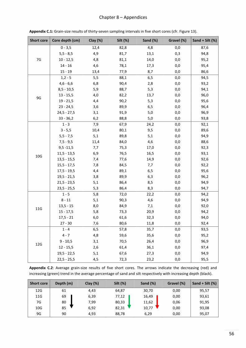
Chapter 8 – Appendices
56
Appendix C.1: Grain-size results of thirty-seven sampling intervals in five short cores (cfr. Figure 13).
Short core Core depth (cm) Clay (%) Silt (%) Sand (%) Gravel (%) Sand + Silt (%)
7G
0 - 3,5 12,4 82,8 4,8 0,0 87,6
5,5 - 8,5 4,9 81,7 13,1 0,3 94,8
10 - 12,5 4,8 81,1 14,0 0,0 95,2
14 - 16 4,6 78,1 17,3 0,0 95,4
15 - 19 13,4 77,9 8,7 0,0 86,6
9G
1,2 - 5 5,5 88,1 6,5 0,0 94,5
4,6 - 6,6 6,8 90,4 2,8 0,0 93,2
8,5 - 10,5 5,9 88,7 5,3 0,0 94,1
13 - 15,5 4,0 82,2 13,7 0,0 96,0
19 - 21,5 4,4 90,2 5,3 0,0 95,6
23 - 24,5 3,6 89,9 6,5 0,0 96,4
24,5 - 27,5 3,1 91,9 5,0 0,0 96,9
33 - 36,2 6,2 88,8 5,0 0,0 93,8
10G
1 - 3 7,9 67,9 24,2 0,0 92,1
3 - 5,5 10,4 80,1 9,5 0,0 89,6
5,5 - 7,5 5,1 89,8 5,1 0,0 94,9
7,5 - 9,5 11,4 84,0 4,6 0,0 88,6
9,5 -11,5 7,7 75,3 17,0 0,0 92,3
11,5 - 13,5 6,9 76,5 16,5 0,0 93,1
13,5 - 15,5 7,4 77,6 14,9 0,0 92,6
15,5 - 17,5 7,8 84,5 7,7 0,0 92,2
17,5 - 19,5 4,4 89,1 6,5 0,0 95,6
19,5 - 21,5 3,8 89,9 6,3 0,0 96,2
21,5 - 23,5 5,1 86,4 8,5 0,0 94,9
23,5 - 25,5 5,3 86,4 8,3 0,0 94,7
11G
1 - 5 5,8 72,0 22,2 0,0 94,2
8 - 11 5,1 90,3 4,6 0,0 94,9
13,5 - 15 8,0 84,9 7,1 0,0 92,0
15 - 17,5 5,8 73,3 20,9 0,0 94,2
17,5 - 21 6,0 61,6 32,3 0,0 94,0
27 - 30 7,6 80,6 11,8 0,0 92,4
12G
1 - 4 6,5 57,8 35,7 0,0 93,5
4 - 7 4,8 59,6 35,6 0,0 95,2
9 - 10,5 3,1 70,5 26,4 0,0 96,9
12 - 15,5 2,6 61,4 36,1 0,0 97,4
19,5 - 22,5 5,1 67,6 27,3 0,0 94,9
22,5 - 25,5 4,5 72,3 23,2 0,0 95,5
Appendix C.2: Average grain-size results of five short cores. The arrows indicate the decreasing (red) and
increasing (green) trend in the average percentage of sand and silt respectively with increasing depth (black).
Short core Depth (m) Clay (%) Silt (%) Sand (%) Gravel (%) Sand + Silt (%)
12G 61 4,43 64,87 30,70 0,00 95,57
11G 69 6,39 77,12 16,49 0,00 93,61
7G 80 7,99 80,33 11,62 0,06 91,95
10G 85 6,92 82,31 10,77 0,00 93,08
9G 90 4,93 88,78 6,29 0,00 95,07

Chapter 8 – Appendices
57
Appendix D: Grain-size results of nineteen profundal surface sediments. The different observations discussed
in section 5.1.3 are indicated by superscripts (1
observation 1, 2
observation 2, 3
observation 3).
Sample Depth (m) Clay (%) Silt (%) Sand (%) Gravel (%) Sand + Silt (%)
2G2
90,7 4,5 90,0 5,5 0,0 95,5
5G3
54,9 4,4 85,4 10,2 0,0 95,6
6G2
91,6 5,9 78,8 15,4 0,0 94,1
7G2
91,3 4,6 71,6 23,8 0,0 95,4
8G2
88,5 4,0 71,3 24,7 0,0 96,0
9G2
75 7,8 49,9 40,7 1,6 90,6
10G1
64,7 13,1 37,3 49,6 0,0 86,9
11G1
32,8 21,6 41,4 37,0 0,0 78,4
12G* 72,7 5,4 67,0 27,1 0,4 94,1
14G3
62 4,7 84,4 11,0 0,0 95,3
15G3
60,8 2,5 68,3 29,2 0,0 97,5
16G3
68,2 2,9 72,5 23,5 1,0 96,0
17G3
89,1 4,0 84,8 11,1 0,0 96,0
18G3
86,1 4,0 86,7 9,3 0,0 96,0
19G* 90,4 3,3 86,0 10,7 0,0 96,7
20G1
89,2 20,3 65,9 13,8 0,0 79,7
21G1
78,7 27,6 60,3 12,1 0,0 72,4
24G3
89 3,9 74,7 21,3 0,0 96,1
25G3
73,4 2,8 78,3 18,8 0,1 97,1
* Not included in any observation
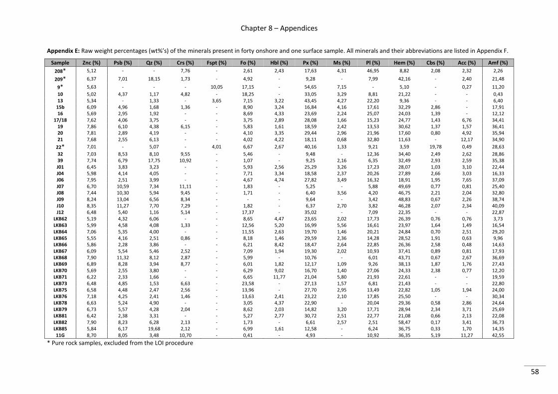
Chapter 8 – Appendices
58
Appendix E: Raw weight percentages (wt%’s) of the minerals present in forty onshore and one surface sample. All minerals and their abbreviations are listed in Appendix F.
Sample Znc (%) Psb (%) Qz (%) Crs (%) Fspt (%) Fo (%) Hbl (%) Px (%) Ms (%) Pl (%) Hem (%) Cbs (%) Acc (%) Amf (%)
208* 5,12 - - 7,76 - 2,61 2,43 17,63 4,31 46,95 8,82 2,08 2,32 2,26
209* 6,37 7,01 18,15 1,73 - 4,92 - 9,28 - 7,99 42,16 - 2,40 21,48
9* 5,63 - - - 10,05 17,15 - 54,65 7,15 - 5,10 - 0,27 11,20
10 5,02 4,37 1,17 4,82 - 18,25 - 33,05 3,29 8,81 21,22 - - 0,43 13 5,34 - 1,33 - 3,65 7,15 3,22 43,45 4,27 22,20 9,36 - - 6,40
15b 6,09 4,96 1,68 1,36 - 8,90 3,24 16,84 4,16 17,61 32,29 2,86 - 17,91 16 5,69 2,95 1,92 - - 8,69 4,33 23,69 2,24 25,07 24,03 1,39 - 12,12
17/18 7,62 4,06 3,75 - - 3,75 2,89 28,08 1,66 15,23 24,77 1,43 6,76 34,41 19 7,86 6,10 4,38 6,15 - 5,83 1,61 18,59 2,42 13,53 30,62 1,37 1,57 36,41 20 7,81 2,89 4,19 - - 4,10 3,35 29,44 2,96 21,96 17,60 0,80 4,92 35,94 21 7,68 2,55 6,13 - - 4,02 4,22 18,11 0,68 32,80 11,63 - 12,17 34,90
22* 7,01 - 5,07 - 4,01 6,67 2,67 40,16 1,33 9,21 3,59 19,78 0,49 28,63
32 7,03 8,53 8,10 9,55 - 5,46 - 9,48 - 12,36 34,40 2,49 2,62 28,86 39 7,74 6,79 17,75 10,92 - 1,07 - 9,25 2,16 6,35 32,49 2,93 2,59 35,38 J01 6,45 3,83 3,23 - - 5,93 2,56 25,29 3,26 17,23 28,07 1,03 3,10 22,44 J04 5,98 4,14 4,05 - - 7,71 3,34 18,58 2,37 20,26 27,89 2,66 3,03 16,33 J06 7,95 2,51 3,99 - - 4,67 4,74 27,82 3,49 16,32 18,91 1,95 7,65 37,09 J07 6,70 10,59 7,34 11,11 - 1,83 - 5,25 - 5,88 49,69 0,77 0,81 25,40 J08 7,44 10,30 5,94 9,45 - 1,71 - 6,40 3,56 4,20 46,75 2,21 2,04 32,80 J09 8,24 13,04 6,56 8,34 - - - 9,64 - 3,42 48,83 0,67 2,26 38,74 J10 8,35 11,27 7,70 7,29 - 1,82 - 6,37 2,70 3,82 46,28 2,07 2,34 40,09 J12 6,48 5,40 1,16 5,14 - 17,37 - 35,02 - 7,09 22,35 - - 22,87
LKB62 5,19 4,32 6,06 - - 8,65 4,47 23,65 2,02 17,73 26,39 0,76 0,76 3,73 LKB63 5,99 4,58 4,08 1,33 - 12,56 5,20 16,99 5,56 16,61 23,97 1,64 1,49 16,54 LKB64 7,06 5,35 4,00 - - 11,55 2,63 19,70 1,46 20,21 24,84 0,70 2,51 29,20 LKB65 5,55 4,16 2,51 0,86 - 8,18 1,46 29,59 2,36 14,28 28,52 1,91 0,63 9,96 LKB66 5,86 2,28 3,86 - - 6,21 8,42 18,47 2,64 22,85 26,36 2,58 0,48 14,63 LKB67 6,09 5,54 5,46 2,52 - 7,09 1,94 19,30 2,02 10,93 37,41 0,89 0,81 17,93 LKB68 7,90 11,32 8,12 2,87 - 5,99 - 10,76 - 6,01 43,71 0,67 2,67 36,69 LKB69 6,89 8,28 3,94 8,77 - 6,01 1,82 12,17 1,09 9,26 38,13 1,87 1,76 27,43 LKB70 5,69 2,55 3,80 - - 6,29 9,02 16,70 1,40 27,06 24,33 2,38 0,77 12,20 LKB71 6,22 2,33 1,66 - - 6,65 11,77 21,04 5,80 21,93 22,61 - - 19,59 LKB73 6,48 4,85 1,53 6,63 - 23,58 - 27,13 1,57 6,81 21,43 - - 22,80 LKB75 6,58 4,48 2,47 2,56 - 13,96 - 27,70 2,95 13,49 22,82 1,05 1,94 24,00 LKB76 7,18 4,25 2,41 1,46 - 13,63 2,41 23,22 2,10 17,85 25,50 - - 30,34 LKB78 6,63 5,24 4,90 - - 3,05 4,37 22,90 - 20,04 29,36 0,58 2,86 24,64 LKB79 6,73 5,57 4,28 2,04 - 8,62 2,03 14,82 3,20 17,71 28,94 2,34 3,71 25,69 LKB81 6,42 2,38 3,31 - - 5,27 2,77 30,72 2,51 22,77 21,08 0,66 2,13 22,08 LKB82 7,90 8,23 6,28 2,13 - 1,73 - 6,61 2,57 2,51 58,47 0,17 3,41 36,73 LKB85 5,84 6,17 19,68 2,12 - 6,99 1,61 12,58 - 6,24 36,75 0,33 1,70 14,35 11G 8,70 8,05 3,48 10,70 - 0,41 - 4,93 - 10,92 36,35 5,19 11,27 42,55
* Pure rock samples, excluded from the LOI procedure

Chapter 8 – Appendices
59
Appendix F: Explanatory list of different mineral phases found in forty-one XRD samples (Anthony et al., 2003).
Pseudobrookite (Psb): formed by pneumatolytic6 processes in titanium-rich basalts. It can be associated with
i.a. hematite and quartz and occurs i.a. on Mt. Kilimanjaro, Tanzania.
Quartz (Qz): second most abundant and most commonly distributed mineral in Earth’s continental crust, i.a.
occurring in sandstones, granites and less abundant in other rock types. It is part of the silica polymorph
group (i.e. Tridymite, Cristobalite,…) and is associated with many other species e.g. feldspars, carbonates.
Cristobalite (Crs): low- to high-temperature polymorph of silica (< or > 268°C), formed during a late-
crystallizing phase in basaltic igneous rocks or by recrystallization from siliceous sedimentary rocks.
Feldspathoids (Fspt): minerals in this group resemble feldspars, but have a different structure and a much
lower silica content. Their occurrence is limited to rare and unusual types of volcanic rocks and they are also
seldom found in rocks containing primary silica. Analcime and nepheline are examples of feldspathoids.
Forsterite (Fo): magnesium-rich end-member of olivine. It occurs i.a. in mafic and ultramafic igneous rocks
and can be associated with e.g. plagioclase, diopside, augite and several other minerals.
Hornblende (Hbl): consists of two end-members, namely ferrohornblende (Fe2+
-rich) and
magnesiohornblende (Mg-rich). It is generally referred to as a dark amphibole and commonly occurs in
amphibolites formed by metamorphism of basalts. Furthermore, it is also an important constituent in many
igneous rocks such as basalts, andesites and granites. It has a very widespread distribution.
Pyroxenes (Px): this group of important rock-forming minerals is abundantly present in mafic to ultramafic
igneous (e.g. basalts and gabbro’s) and metamorphic rocks. Together with olivine, they are the main
constituents of Earth’s upper mantle. Their distribution is widespread and they can be associated with
amphiboles, olivine and feldspars. Diopside and augite are examples of pyroxenes present around Lake Challa.
Muscovite (Mu): most common and widely distributed mica, occurring in igneous, metamorphic and
sedimentary regimes. It is commonly found in i.a. phyllites, schists, gneisses and granites and is mainly
associated with quartz, plagioclase and potassium-rich feldspars.
Plagioclases (Pl): this large group of minerals is part of the feldspars, which are the most abundant minerals
in Earth’s continental crust. Moreover, plagioclase represents a continuous solid solution series7 that ranges
between end-members albite (Na-rich) and anorthite (Ca-rich). They are widely distributed and occur in
igneous rocks of intermediate silica content such as diorites, andesites, granites and gneisses. Oligoclase and
andesine, both members of the plagioclase feldspar series, are mainly found around Lake Challa.
Hematite (Hem): this mineral is one of several iron oxides that occur widespread in nature. Its formation can
be the result of volcanic activity, but clay-sized hematite crystals can also occur as secondary minerals formed
by weathering processes in soil samples. Along with other iron oxides such as magnetite and goethite,
hematite is responsible for the red (lateritic) to greyish (volcanic) colour of many tropical weathered soils.
Carbonates (Cbs): this group comprises a large amount of crystals, but around Lake Challa only minor
amounts of lime, dolomite and magnesite are found (Table 1). These minerals are associated with each other
and occur in i.a igneous rocks or rocks altered by diagenesis or metamorphism. They are of minor importance
for this study.
Accessories (Acc): as the arbitrary name of this group indicates, the minerals within are accessory, implying
that their presence around Lake Challa cannot clearly be explained. As with the carbonates, they are of minor
importance for this study, yet a remarkable observation is discussed in Chapter 5. The minerals akermanite
and mayenite are included in this group and both can be the result of high-temperature alterations of
siliceous limestones.
6 A process of rock alteration or mineral formation affected by gaseous emissions from solidifying magma
(Bates and Jackson, 1984). 7 Plagioclase feldspar series: Anorthite, Bytownite, Labradorite, Andesine, Oligoclase and Albite.