variable rare disasters: an exactly solved …pages.stern.nyu.edu/~xgabaix/papers/tenpuzzles.pdf ·...
TRANSCRIPT

VARIABLE RARE DISASTERS: AN EXACTLY SOLVEDFRAMEWORK FOR TEN PUZZLES IN MACRO-FINANCE∗
XAVIER GABAIX
This article incorporates a time-varying severity of disasters into the hy-pothesis proposed by Rietz (1988) and Barro (2006) that risk premia result fromthe possibility of rare large disasters. During a disaster an asset’s fundamentalvalue falls by a time-varying amount. This in turn generates time-varyingrisk premia and, thus, volatile asset prices and return predictability. Usingthe recent technique of linearity-generating processes, the model is tractableand all prices are exactly solved in closed form. In this article’s framework,the following empirical regularities can be understood quantitatively: (i) equitypremium puzzle; (ii) risk-free rate puzzle; (iii) excess volatility puzzle; (iv)predictability of aggregate stock market returns with price-dividend ratios; (v)often greater explanatory power of characteristics than covariances for assetreturns; (vi) upward-sloping nominal yield curve; (vii) predictability of futurebond excess returns and long-term rates via the slope of the yield curve; (viii)corporate bond spread puzzle; (ix) high price of deep out-of-the-money puts; and(x) high put prices being followed by high stock returns. The calibration passesa variance bound test, as normal-times market volatility is consistent with thewide dispersion of disaster outcomes in the historical record. The model extendsto a setting with many factors and to Epstein-Zin preferences. JEL Codes: E43,E44, G12.
I. INTRODUCTION
There has been a revival of a hypothesis proposed by Rietz(1988) that the possibility of rare disasters, such as economicdepressions or wars, is a major determinant of asset risk premia.Indeed, Barro (2006) has shown that internationally, disastershave been sufficiently frequent and large to make Rietz’s pro-posal viable and account for the high risk premium on equities.Additionally, the recent economic crisis has given disaster risk arenewed salience.
The rare disaster hypothesis is almost always formulatedwith constant severity of disasters. This is useful for thinking
∗I thank Alex Chinco, Esben Hedegaard, Farzad Saidi, and Rob Tumarkinfor excellent research assistance. For helpful comments, I thank five refer-ees and Robert Barro (the editor), David Chapman, Alex Edmans, EmmanuelFarhi, Francois Gourio, Christian Julliard, Sydney Ludvigson, Anthony Lynch,Thomas Philippon, JoseScheinkman, JoseUrsua, StijnvanNieuwerburgh, AdrienVerdelhan, Stan Zin, and seminar participants at AFA, Chicago GSB, Duke, Har-vard, Minnesota Workshop in Macro Theory, MIT, NBER, NYU, Paris School ofEconomics, Princeton, Texas FinanceFestival, UCLA, andWashingtonUniversityat Saint Louis. I thank Robert Barro, Stephen Figlewski, Arvind Krishnamurthy,Jose Ursua, Annette Vissing-Jorgensen, andHaoZhou fortheirdata, andthe NSF(grant SES-0820517) for support.
c© The Author(s) 2012. Published by Oxford University Press, on the behalf of Presidentand Fellows of Harvard College. All rights reserved. For Permissions, please email: [email protected] Quarterly Journal of Economics (2012) 127, 645–700. doi:10.1093/qje/qjs001.Advance Access publication on March 14, 2012.
645
at New
York U
niversity School of Law
on May 1, 2012
http://qje.oxfordjournals.org/D
ownloaded from

646 QUARTERLY JOURNAL OF ECONOMICS
about averages but cannot account for some key features of assetmarkets, such as volatile price-dividend ratios for stocks, volatilebond risk premia, and return predictability. In this article, I for-mulatea variable-severityversionof theraredisasters hypothesisandinvestigatetheimpact oftime-varyingdisasterseverityontheprices of stocks and bonds as well as on the predictability of theirreturns.1
I show that many asset puzzles can be qualitatively under-stood using this model. I then demonstrate that a parsimoniouscalibration allows one to understand the puzzles quantitatively,providedthat real andnominal variables aresufficientlysensitiveto disasters (which I argue is plausible below).
The proposed framework allows for a very tractable modelof stocks and bonds in which all prices are in closed form. Inthis setting, the following patterns are not puzzles but emergenaturally when the present model has just two shocks: a real onefor stocks and a nominal one for bonds.2
I.A. Stock Market: Puzzles about the Aggregates
1. Equity premium puzzle: The standard consumption-basedmodel with reasonable relative risk aversion (less than 10)predicts a too low equity premium (Mehra and Prescott1985).
2. Risk-free rate puzzle: Increasing risk aversion leads to atoo high risk-free rate in the standard model (Weil 1989).3
3. Excess volatility puzzle: Stock prices seem more volatilethan warranted by a model with a constant discount rate(Shiller 1981).
4. Aggregate return predictability: Future aggregate stockmarket returns are partly predicted by price/dividend(P/D) and similar ratios (Campbell and Shiller 1998).
I.B. Stock Market: Puzzles about the Cross-Section of Stocks
5. Characteristics vs. covariances puzzle: Stock characteris-tics (e.g., the P/D ratio) often predict future returns as well
1. A later companion paper, Farhi andGabaix (2011), studies exchange rates.A brief introductionis Gabaix(2008), but almost all results appearhereforthefirsttime.
2. I mention just a few references, but most puzzles have been documentedby numerous authors.
3. For this andthe above puzzle, the article simply imports from Rietz (1988),Longstaff and Piazzesi (2004), and Barro (2006).
at New
York U
niversity School of Law
on May 1, 2012
http://qje.oxfordjournals.org/D
ownloaded from

VARIABLE RARE DISASTERS 647
as or better than covariances with risk factors (Daniel andTitman 1997).
I.C. Nominal Bond Puzzles
6. Yieldcurveslopepuzzle: Thenominal yieldcurveslopes upon average. The premium of long-term yields over short-term yields is too high to be explained by a traditionalRBC model. This is thebondversionof theequitypremiumpuzzle (Campbell 2003).
7. Long-term bond return predictability: A high slope of theyieldcurvepredicts highexcess returns onlong-termbonds(Macaulay 1938; Fama and Bliss 1987; Campbell andShiller 1991).
8. Credit spread puzzle: Corporate bond spreads are seem-ingly higher than warranted by historical default rates(Almeida and Philippon 2007).
I.D. Options Puzzles
9. Deep out-of-the-money puts have higher prices thanpredicted by the Black-Scholes model (Jackwerth andRubinstein 1996).
10. When prices of puts on the stock market index are high,so are its future returns (Bollerslev, Tauchen, and Zhou2009).
To understand the economics of the model, first considerbonds. Consistent with the empirical evidence reviewed shortly,a disaster leads on average to a positive jump in inflation in themodel. This has a greater detrimental impact on long-term bonds,so they command a high risk premium relative to short-termbonds. This explains the upward slope of the nominal yield curve.Next, suppose that the size of the expected jump in inflation itselfvaries. Then, the slope of the yield curve will vary and predictexcess bond returns. A high slope will mean-revert and, thus,predicts a drop in the long rate and high returns on long-termbonds. This mechanismaccounts formanystylizedfacts onbonds.
The same mechanism is at work for stocks. Suppose thata disaster reduces the fundamental value of a stock by atime-varying amount. This yields a time-varying risk premiumthat generates a time-varyingprice-dividendratioandthe“excessvolatility” of stock prices. It also makes stock returns predictablevia measures such as the price-dividend ratio. When agents
at New
York U
niversity School of Law
on May 1, 2012
http://qje.oxfordjournals.org/D
ownloaded from

648 QUARTERLY JOURNAL OF ECONOMICS
perceive the severity of disasters as low, price-dividend ratios arehigh and future returns are low.
The model’s mechanism also impacts disaster-related assetssuch as corporate bonds and options. If high-quality corporatebonds default mostlyduringdisasters, thentheyshouldcommanda high premium that cannot be accounted for by their behaviorduring normal times. The model alsogenerates option prices witha “volatility smirk,” that is, a high put price (and, thus, impliedvolatility) for deep out-of-the-money put options.
After laying out the framework and solving it in closed form,I calibrate it. The values for disasters are essentially taken fromBarro and Ursua’s (2008) analysis of many countries’ disasters,defined as drops in GDP or consumption of 10% or more. Thecalibration yields results for stocks, bonds, and options consistentwith empirical values. The volatilities of the expectation aboutdisaster sizes are very hard to measure directly. However, thecalibration generates a steady-state dispersion of anticipationsthat is lower than the dispersion of realized values. This isshown by “dispersion ratio tests” in the spirit of Shiller (1981),which are passed by the disaster model. By that criterion, thecalibrated values in the model appear reasonable. Importantly,they generate a series of fine quantitative predictions. Hence, themodel calibrates quite well.
So far, asset price movements come from changes in howbadlytheasset will performif a disasterhappens (i.e., movementsin the asset-specific recovery). The power utility model allows ustothink about that quantitatively. However, as foundby previousauthors (see, for instance, Barro 2009), the power utility modelhas one important anomalous feature: when the disaster prob-ability goes up, even though risk premia increase, the safe ratedecreases so much that asset prices tend to go up. To counteractthe strong movement in the short rate, it is useful to have anEpstein-Zin model, which basically weakens this movement, aspeople’s savings behavior is decoupled from their risk aversion.I extend the model to Epstein-Zin preferences only later in thearticle, as the machinery is substantially more complex. Formovements in asset-specific fears, the Epstein-Zin model leadsto very similar predictions. However, it makes arguably betterpredictions formovements indisasterprobability. Hence, I recom-mend the basic power utility model for many asset pricing issues,such as the volatility of stocks, bonds, and the predictability oftheir returns, but to study the impact of movements in disaster
at New
York U
niversity School of Law
on May 1, 2012
http://qje.oxfordjournals.org/D
ownloaded from

VARIABLE RARE DISASTERS 649
probability, I recommend paying the somewhat higher cost ofusing the Epstein-Zin model.
Throughout this article, I use the class of “linearity-generating” (LG) processes (Gabaix 2009), which was motivatedby the present article. That class keeps all expressions in closedform. The entire article could be rewritten with other processes(e.g., affine-yield models) albeit with considerably more compli-cated algebra and the need to resort to numerical solutions. TheLG class and the affine class yield the same expression to a first-order approximation. The use of the LG processes should thus beviewed as a mere analytical convenience.
Relation to the Literature. A few papers address the issueof time-varying disasters. Longstaff and Piazzesi (2004) consideran economy with constant severity of disasters, but in which stockdividends are a variable, mean-reverting share of consumption.They find a high equity premium and highly volatile stock re-turns. Veronesi (2004) considers a model in which investors learnabout a world economy that follows a Markov chain through twopossible economic states, one of which may be a disaster state.His model yields GARCH effects and apparent “overreaction.”Weitzman (2007) provides a Bayesian view that the main riskis model uncertainty, as the true volatility of consumption maybe much higher than the sample volatility.4 Unlike the presentwork, all of those papers neither consider bonds nor study returnpredictability.
After the present paper was circulated, Wachter (2009) pro-posed a different model, based on Epstein-Zin utilities, wherevaluation movements come solely from the stochastic probabilityof disasters and which analyzes stocks and the short-term rate,but not nominal bonds. The present article, in contrast, allowsthe stochasticity to come both from movements in the probabilityof disasters and from the expected recovery rate of various assets,and can work with power utility as well as Epstein-Zin utility.Importantly, it is conceived to easily handle several assets, suchas nominal bonds and stocks (as in this article), stocks withdifferent timing of cash flows (Binsbergen, Brandt, and Koijen
4. Another relatedliterature explores the idea that fear of medium-frequency(e.g., yearly) market crashes (rather than macroeconomic disasters) is impor-tant for risk premia. Such high-frequency extreme events could be due to thetrades of large funds trading under limited liquidity (Gabaix et al. 2003, 2006;Brunnermeier, Nagel, and Pedersen 2008).
at New
York U
niversity School of Law
on May 1, 2012
http://qje.oxfordjournals.org/D
ownloaded from

650 QUARTERLY JOURNAL OF ECONOMICS
forthcoming), particular corporate sectors (Ghandi and Lustig2011), and exchange rates (Farhi and Gabaix 2011). This choiceis motivated by the empirical evidence which shows that severalfactors are needed to explain risk premia (Fama and French1993) across stocks and bonds. It is useful to have asset-specificshocks, as single-factor models generate perfect correlations ofrisk premia across assets, while empirically valuation ratios arenot highly correlated across assets (see Section IV.A).
Within the class of rational, representative-agent frame-works that deliver time-varying risk premia, the variable raredisasters model may be a third workable framework, along withthe external-habit model of Campbell and Cochrane (CC 1999)andthelong-runriskmodel of Bansal andYaron(BY 2004). Thesehave proven to be two very useful and influential models. Still,the reader might ask: why do we need another model of time-varying risk premia? The variable rare disasters framework hasseveral useful features, besides the obvious feature that disasterrisk might be substantially crucial for financial prices.
First, as emphasized by Barro (2006), the model uses thetraditional isoelasticexpected utility framework like the majorityof models in macroeconomictheory. CC and BY use more complexutility functions with external habit and Epstein and Zin (1989)utility, which are harder to embed in macroeconomic models. InGabaix (2011) (see also Gourio 2011), I show how the presentmodel (in an endowment economy) can be directly mapped into aproduction economy with traditional real business cycle features.Hence, the rare-disasters idea brings us closer to the long-soughtunification of macroeconomics and finance. Second, the modelmakes different predictions for the behavior of “tail-sensitive”assets, such as deep out-of-the-money options and high-yieldcorporate bonds—broadly speaking, the model naturally predictsthat such assets command very high premia. Third, the model isparticularly tractable. Stock and bond prices have linear closedforms. As a result, asset prices and premia can be derived andanalytically understood without recourse to simulations. Fourth,the model easily accounts for some facts that are hard togeneratein the CC andBY models. In my proposedmodel, “characteristics”(such as P/D ratios) predict future stock returns better thanmarket covariances, which is virtually impossible to generate inthe CC and BY frameworks. The model also generates a low cor-relation between consumption growth and stock market returns,which is also hard to achieve in the CC and BY models.
at New
York U
niversity School of Law
on May 1, 2012
http://qje.oxfordjournals.org/D
ownloaded from

VARIABLE RARE DISASTERS 651
There is a well-developed literature that studies jumps par-ticularly with option pricing in mind. Using options, Liu, Pan,and Wang (2005) calibrate models with constant risk premia anduncertainty aversion, demonstrating the empirical relevance ofrare events in asset pricing. Santa-Clara and Yan (2010) alsouse options to calibrate a model with frequent jumps. Typically,the jumps in these papers happen every few days or months andaffect consumption by moderate amounts, whereas the jumps inthe rare-disasters literature happen perhaps once every 50 yearsand are larger. The authors alsodonot study the impact of jumpson bonds and return predictability.
Section II presents the macroeconomic environment andthe cash-flow processes for stocks and bonds. Section III derivesequilibrium prices. Section IV proposes a calibration and reportsthe model’s implications for stocks, options, and bonds. Section Vdiscusses various extensions of the model, in particular to anEpstein-Zin economy. The Appendix contains notations andsome derivations. An Online Appendix contains supplementaryinformation and extensions.
II. MODEL SETUP
II.A. Macroeconomic Environment
The environment follows Rietz (1988) and Barro (2006), andadds a stochastic probability and severity of disasters. There isa representative agent with utility E0
[∑∞t=0 e−ρt C1−γ
t −11−γ
], where
γ ≥ 0 is the coefficient of relative risk aversion and ρ > 0 is therate of time preference. She receives a consumption endowmentCt. At each period t + 1, a disaster may happen with a probabilitypt. If a disaster does not happen, Ct+1
Ct= egC , where gC is the
normal-time growth rate of the economy. If a disaster happens,Ct+1Ct
= egCBt+1, where Bt+1 > 0 is a random variable.5 For instance,if Bt+1 = 0.8, consumption falls by 20%. To sum up:6
(1)Ct+1
Ct= egC ×
{1 if there is no disaster at t + 1Bt+1 if there is a disaster at t + 1
.
5. Typically, extra i.i.d. noise is added, but given that it never materiallyaffects asset prices, it is omitted here. It could be added without difficulty. Also,countercyclicality of risk premia could easily be added to the model withouthurting its tractability.
6. The consumption drop is permanent. One could add mean-reversion aftera disaster.
at New
York U
niversity School of Law
on May 1, 2012
http://qje.oxfordjournals.org/D
ownloaded from

652 QUARTERLY JOURNAL OF ECONOMICS
The pricing kernel is the marginal utility of consumption Mt =e−ρtC−γt , and follows:
(2)Mt+1
Mt= e−δ ×
{1 if there is no disaster at t + 1B−γt+1 if there is a disaster at t + 1
,
where δ = ρ + γgc, the “Ramsey” discount rate, is the risk-free ratein an economy that would have a zero probability of disasters.The price at t of an asset yielding a stream of dividends (Ds)s≥t
is: Pt =Et[∑
s≥t MsDs]Mt
.
II.B. Setup for Stocks
I consider a typical stock i which is a claim on a stream ofdividends (Dit)t≥0:7
Di,t+1
Dit= egiD
(1 + εD
i.t+1
)(3)
×
{1 if there is no disaster at t + 1Fi,t+1 if there is a disaster at t + 1
,
where εDi,t+1 > −1 is a mean-zero shock that is independent of
the disaster event. It matters only for the calibration of dividendvolatility. In normal times, Dit grows at an expected rate of giD.But if there is a disaster, the dividend of the asset is partiallywiped out following Longstaff and Piazzesi (2004) and Barro(2006): the dividend is multiplied by a random variable Fi,t+1 ≥ 0,which is the recovery rate of the dividend. In other terms, for thisindividual asset i, there can be a partial “default” in a disaster,without any necessary effect on aggregate consumption and thepricing kernel. When Fi,t+1 = 0, the asset is completely destroyedor expropriated. When Fi,t+1 = 1, there is no dividend loss.
To model the time variation in the asset’s recovery rate,I introduce the notion of “resilience” Hit of asset i,
(4) Hit = ptEDt
[B−γt+1Fi,t+1 − 1
],
where ED (resp. END) is the expected value conditionally on adisaster happening at t + 1 (resp. no disaster).8 In (4), pt and B−γt+1
7. There can be many stocks. The aggregate stock market is a priori notaggregate consumption, because the whole economy is not securitized in the stockmarket. Indeed, stock dividends are more volatile than aggregate consumption.
8. Later in the paper, when there is no ambiguity (e.g., for E[B−γt+1
]), I will
drop the D.
at New
York U
niversity School of Law
on May 1, 2012
http://qje.oxfordjournals.org/D
ownloaded from

VARIABLE RARE DISASTERS 653
are economy-wide variables, whereas the resilience and recoveryrate Fi,t+1 are stock-specific though typically correlated with therest of the economy.
When the asset is expected to do well in a disaster (highFi,t+1), Hit is high—investors are optimisticabout the asset. In thecross-section, an asset with higher resilience Hit is safer than onewith lowresilience. As is intuitive, assets with high resilience willcommand low risk premia.
I specify the dynamics of Hit directly rather than through theindividual components pt, Bt+1, andFi,t+1. I split resilience Hit intoa constant part Hi∗ and a variable part Hit:
Hit = Hi∗ + Hit,
and I postulate the following linearity-generating (Gabaix 2009)process for the variable part Hit:
(5) Hi,t+1 =1 + Hi∗
1 + Hite−φH Hit + εH
i,t+1,
where EtεHi,t+1 = 0 and εH
i,t+1, εDt+1, and the disaster event are uncor-
related variables.To interpret (5), observe that to the leading order, it implies
that Hi,t+1 ' e−φH Hit +εHi,t+1 (as Hit hovers aroundHi∗,
1+Hi∗1+Hit
is close
to 1): Hit mean-reverts to 0 at a speed φH, but has innovations ateveryperiod. Totheleadingorder, theprocess is anautoregressiveAR(1) process. However, this is a “twisted”AR(1); the“twist”term1+Hi∗1+Hit
makes prices linear in the factors and independent of thefunctional form of the noise.9
Economically, Hit does not jump if there is a disaster. How-ever, one can imagine, for instance, that resilience falls in adisaster. Such a feature could easily be added in the form of anextra negative jump in (5) in case of a disaster. Everything wouldgo through qualitatively, though in addition, equities would beeven riskier. However, to keep the model parsimonious, I shrinkfrom postulating that extra feature.
I turn to bonds.
9. The noise εHt+1 can be heteroskedastic, but its variance need not be spelled
out, as it does not enter into the prices. However, the process needs to sat-isfy Hit
(1+Hi∗)≥ e−φH − 1 for it to be stable, and also Hit ≥ −p − Hi∗ to
ensure Fit ≥ 0. Hence, the variance needs to vanish in a right neighborhoodmax
((e−φH − 1
)(1 + Hi∗) ,−p−Hi∗
)(see Gabaix 2009).
at New
York U
niversity School of Law
on May 1, 2012
http://qje.oxfordjournals.org/D
ownloaded from

654 QUARTERLY JOURNAL OF ECONOMICS
II.C. Setup for Bonds
The twomost salient facts on nominal bonds are arguably thefollowing. First, the nominal yield curve slopes up on average,that is, long-term rates are higher than short-term rates (e.g.,Campbell 2003, Table VI). Second, there are stochastic bondrisk premia. The risk premium on long-term bonds increaseswith the difference between the long-term rate and the short-term rate (Fama and Bliss 1987; Campbell and Shiller 1991;Cochrane and Piazzesi 2005). These facts are considered to bepuzzles because they are not derived from standard macroeco-nomic models, which generate risk premia that are too small(Mehra and Prescott 1985).
I propose the following explanation. When a disaster occurs,inflationincreases (onaverage). Sinceveryshort-termbills arees-sentially immune to inflation risk and long-term bonds lose valuewhen inflation is higher, long-term bonds are riskier, sothey yielda higher risk premium. Thus, the yieldcurve slopes up. Moreover,the magnitude of the surge in inflation is time-varying, whichgenerates a time-varying bond premium. If that bond premiumis mean-reverting, it generates the Fama-Bliss puzzle. Note thatthis explanation does not hinge on the specifics of the disastermechanism. The advantage of the disaster framework is that itallows for formalizing and quantifying the idea in a simple way.
Several authors have models where inflation is higher in badtimes, whichmakes theyieldcurveslopeup. Anearlierunificationof several puzzles is provided by Wachter (2006), who studies aCampbell and Cochrane (1999) model with extra nominal shocks,and concludes that it explains an upward-sloping yield curve andthe Campbell and Shiller (1991) findings. The Brandt and Wang(2003) study is also a Campbell and Cochrane (1999) model, butone where risk aversion depends directly on inflation. Bansaland Shaliastovich (2009) build on Bansal and Yaron (2004). InPiazzesi and Schneider (2007), inflation also rises in bad times,although in a very different model. Finally, Dai and Singleton(2002) and Duffee (2002) present econometric frameworks thatdeliver the Fama-Bliss and Campbell-Shiller results.
I decompose trend inflation It as It = I∗+ It, where I∗ is itsconstant part and It is its variable part. The variable part ofinflation follows the process:
(6) It+1 =1− I∗1− It
∙(
e−φI It + 1{Disaster at t+1}Jt
)+ εI
t+1,
at New
York U
niversity School of Law
on May 1, 2012
http://qje.oxfordjournals.org/D
ownloaded from

VARIABLE RARE DISASTERS 655
where εIt+1 has mean 0 and is uncorrelated with the realization of
a disaster. This equation means, first, that if there is no disaster,EtIt+1= 1−I∗
1−Ite−φI It ' e−φI It, that is, inflationfollows theLG-twisted
autoregressive process (Gabaix 2009). Inflation mean-reverts at arate φI, with the LG twist 1−I∗
1−Itto ensure tractability. In addition,
in case of a disaster, inflation jumps by an amount Jt, decomposedinto Jt = J∗ + Jt, where J∗ is the baseline jump in inflation and Jt
is the mean-reverting deviation of the jump size from baseline.This jump in inflation makes long-term bonds particularly risky.It follows atwistedautoregressiveprocess and, forsimplicity, doesnot jump during crises:
(7) Jt+1 =1− I∗1− It
e−φJ Jt + εJt+1,
where εJt+1 has mean 0. εJ
t+1 is uncorrelated with disasters but canbe correlated with innovations in It.
A few more notations are useful. I define H$ = ptEt[F$,t+1B−γt+1 − 1
], where F$,t+1 is one minus the default rate on
bonds (later this will be useful to differentiate government fromcorporate bonds). For simplicity, I assume that H$ is a constant:there will be much economics coming solely from the variations ofIt. I call πt the variable part of the bond risk premium:
(8) πt ≡ptEt
[B−γt+1F$,t+1
]
1 + H$Jt.
The second notation is only useful when the typical jump ininflation J∗ is not zero, and the reader is invited to skip it in thefirst reading. I parametrize J∗ in terms of a variable κ ≤ 1−e−φI
2 ,called the inflation disaster risk premium:10
(9)ptEt
[B−γt+1F$,t+1
]J∗
1 + H$= (1− I∗)κ
(1− e−φI − κ
),
that is, inthecontinuous timelimit: ptEt[B−γt+1F$,t+1
]J∗=κ (φI − κ).
A high κ means a high central jump in inflation if there isa disaster. For most of the paper it is enough to think thatJ∗ = κ = 0.
10. Calculating bond prices in a linearity-generating process sometimes in-volves calculating the eigenvalues of its generator. I presolve by parameterizingJ∗ by κ. The upper bound on κ implicitly assumes that J∗ is not too large.
at New
York U
niversity School of Law
on May 1, 2012
http://qje.oxfordjournals.org/D
ownloaded from

656 QUARTERLY JOURNAL OF ECONOMICS
II.D. Expected Returns
I conclude the presentation of the economy by stating a gen-eral lemma about the expected returns.
LEMMA 1. (Expected returns) Consider an asset i and call ri,t+1
the asset’s return. Then, the expected return of the asset at t,conditional on no disasters, is:
(10) reit =
11− pt
(eδ − ptE
Dt
[B−γt+1 (1 + ri,t+1)
])− 1.
In the limit of small time intervals,
(11) reit = δ− ptE
Dt
[B−γt+1 (1 + ri,t+1)− 1
]= rf − ptE
Dt
[B−γt+1ri,t+1
],
where rf is the real risk-free rate in the economy:
(12) rf = δ − ptEDt
[B−γt+1 − 1
].
The unconditional expected return is (1− pt) reit + ptED
t [ri,t+1].
Proof. It comes fromtheEulerequation, 1=Et [(1 + ri,t+1)Mt+1/Mt],that is:
1 = e−δ{(1− pt) ∙ (1 + reit)︸ ︷︷ ︸
No disaster term
+ pt ∙ EDt
[B−γt+1 (1 + ri,t+1)
]
︸ ︷︷ ︸Disaster term
}. �
Equation (10) indicates that only the behavior in disasters(the ri,t+1 term) creates a risk premium. It is equal to the risk-adjusted (by B−γt+1) expected capital loss of the asset if there is adisaster.
The unconditional expected return on the asset (i.e., withoutconditioning on no disasters) in the continuous time limit is re
it −ptED
t [ri,t+1]. Barro(2006) observes that the unconditional expectedreturn and the expected return conditional on no disasters arevery close. The possibility of disaster affects primarily the riskpremium, and much less the expected loss.
III. ASSET PRICES AND RETURNS
III.A. Stocks
THEOREM 1. (Stock prices) Let hi∗ = ln (1 + Hi∗) and define δi = δ−giD − hi∗, which will be called the stock’s effective discountrate. The price of stock i is:
at New
York U
niversity School of Law
on May 1, 2012
http://qje.oxfordjournals.org/D
ownloaded from

VARIABLE RARE DISASTERS 657
(13) Pit =Dit
1− e−δi
(
1 +e−δi−hi∗Hit
1− e−δi−φH
)
.
In the limit of short time periods, the price is:
(14) Pit =Dit
δi
(
1 +Hit
δi + φH
)
.
The next proposition links resilience Hit and the equitypremium.
PROPOSITION 1. (Expected stock returns) The expected return onstock i, conditional on no disasters, is:
(15) reit = δ −Hit.
The equity premium (conditional on no disasters) is reit − rf =
ptEt[B−γt+1 (1− Fi,t+1)
], where rf is the risk-free rate derived in
(12). To obtain the unconditional values of these two quanti-ties, subtract ptED
t [1− Fi,t+1].
Proof. If a disaster occurs, dividends are multiplied by Fit. AsHit does not change, 1 + rit = Fit. So returns are, by (11), re
it = δ −pt(Et[B−γt+1Fi,t+1
]− 1)
= δ −Hit. �
As expected, more resilient stocks (assets that do better in adisaster) have a lower ex ante risk premium (a higher Hit). Whenresilience is constant (Hit ≡ 0), equation (14) is Barro (2006)’sexpression. TheP/D ratiois increasinginthestock’s resilience hi∗.
The key advance in Theorem 1 is that it derives the stockprice with a stochastic resilience Hit. More resilient stocks (highHit) have a lower equity premium and a higher valuation. Sinceresilience Hit is volatile, soare price-dividendratios, in a way thatis potentially independent of innovations to dividends. Hence,the model generates a time-varying equity premium and thereis “excess volatility,” that is, volatility of the stocks unrelated to(normal-times) cash-flow news. As the P/D ratio is stationary, itmean-reverts. Thus, the model generates predictability in stockprices. Stocks with a high P/D ratio will have low returns, andstocks with a low P/D ratio will have high returns. SectionIV.B quantifies this predictability. Proposition 11 in the OnlineAppendix extends equation (14) to a world that has variableexpected growth rates of cash flows in addition to variable riskpremia.
at New
York U
niversity School of Law
on May 1, 2012
http://qje.oxfordjournals.org/D
ownloaded from

658 QUARTERLY JOURNAL OF ECONOMICS
III.B. Nominal Government Bonds
THEOREM 2. (Bondprices) In the limit of small time intervals, thenominal short-term rate is rt = δ −H$ + It, and the price of anominal zero-coupon bond of maturity T is:
Z$t (T) = e−(δ−H$+I∗∗)T
(
1−1− e−ψIT
ψI(It − I∗∗)− KTπt
)
,(16)
KT ≡1−e−ψIT
ψI− 1−e−ψJ T
ψJ
ψJ − ψI,
where It is inflation, πt is the bond risk premium, I∗∗ ≡ I∗ + κ,ψI ≡ φI − 2κ, and ψJ ≡ φJ − κ. The discrete-time expressionis in (42).
Theorem 2 gives a closed-form expression for bond prices.As expected, bond prices decrease with inflation and with thebond risk premium. Indeed, expressions 1−e−ψIT
ψIand KT are
non-negative and increasing in bond maturity T. The term1−e−ψIT
ψIIt simply expresses that inflation depresses nominal bond
prices and mean-reverts at a (risk-neutral) rate ψI. The bond riskpremium πt reduces the price all bonds of positive maturity, butnot the short-term rate.
When κ > 0 (resp. κ < 0) inflation typically increases (resp.decreases) during disasters. While φI (resp. φJ) is the speed ofmeanreversionof inflation(resp. of thebondriskpremium, whichis proportional to Jt) under the physical probability, ψI (resp. ψJ)is the speed of mean reversion of inflation (resp. of the bond riskpremium) under the risk-neutral probability.
I calculate expected bond returns, bond forward rates, andyields, again in the limit of small time intervals.
PROPOSITION 2. (Expected bond returns) Conditional on no dis-asters, the short-term real return on a short-term bill isre$t (0) = δ − H$, and the real excess return on the bond of
maturity T is:
re$t (T)− re
$t (0) =1−e−ψIT
ψI(κ (ψI + κ) + πt)
1− 1−e−ψIT
ψI(It − I∗∗) + KTπt
(17)
= T (κ (ψI + κ) + πt) + O (T2) + O (πt, It,κ)2(18)
= TptEt[B−γt+1F$,t+1
]Jt + O (T2) + O (πt, It,κ)
2 .(19)
at New
York U
niversity School of Law
on May 1, 2012
http://qje.oxfordjournals.org/D
ownloaded from

VARIABLE RARE DISASTERS 659
Proof. After a disaster in the next time interval of size dt → 0,inflation jumps by dIt = Jt and πt by 0. By (16), the bond pricejumps by dZ$,t (T) = Z$,t+dt (T − dt) − Z$,t (T) = −e−(δ−H$+I∗∗)T ∙1−e−ψIT
ψIJt + O
(√dt)
. Lemma 1 gives the risk premia,
re$t (T)−re
$t (0)=−ptEt
[
B−γt+1dZ$,t (T)Z$t (T)
]
=1−e−ψIT
ψIptEt
[B−γt+1F$,t+1Jt
]
1− 1−e−ψIT
ψI(It − I∗∗) + KTπt
,
and we conclude using ptEt[B−γt+1F$,t+1Jt
]= κ (φI − κ) + πt =
κ (ψI + κ) + πt. �
Equation (19) shows the first-order value of the bond riskpremium for bonds of maturity T. It is the maturity T of the bondmultiplied by an inflation premium, ptEt
[B−γt+1F$,t+1
]Jt. The infla-
tion premium is equal to the risk-neutral probability of disasters(adjusting for the recovery rate), ptEt
[B−γt+1F$,t+1
], times the jump
in expectedinflation if there is a disaster, Jt. We note that a lowerrecovery rate reduces risk premia, a general feature that we willexplore in greater detail in Section III.D
LEMMA 2. (Bond yields and forward rates) The forward rate,ft (T) ≡ −∂ lnZ$t (T) /∂T, is:
ft (T) = δ −H$ + I∗∗ +e−ψIT (It − I∗∗) + e−ψIT−e−ψJ T
ψJ−ψIπt
1− 1−e−ψIT
ψI(It − I∗∗)− KTπt
(20)
= δ −H$ + I∗∗ + e−ψIT (It − I∗∗) +e−ψIT − e−ψJT
ψJ − ψIπt(21)
+ O (It − I∗∗,πt)2 .
The bond yield is yt (T)=−(lnZ$t(T))
T with Z$t (T) given by (16),and its Taylor expansion is given in (43)–(44).
The forward rate increases with inflation and the bond riskpremia. The coefficient of inflation decays with the speed of meanreversionof inflation, ψI, underthe“risk-neutral”probability. Thecoefficient of the bond premium, πt, is e−ψIT−e−ψJ T
ψJ−ψIand, thus, has
value 0 at both very short and very long maturities and a positivehump shape in between. Very short-term bills, being safe, do notcommand a risk premium, and long-term forward rates are alsoessentiallyconstant (Dybvig, Ingersoll, andRoss 1996). Therefore,the time-varying risk premium only affects intermediate maturi-ties of forwards.
at New
York U
niversity School of Law
on May 1, 2012
http://qje.oxfordjournals.org/D
ownloaded from

660 QUARTERLY JOURNAL OF ECONOMICS
III.C. Options
Let us next study options, which offer a potential way tomeasure disasters. The price of a European one-period put ona stock i with strike K expressed as a ratio to the initial priceis: Vt = Et
[Mt+1Mtmax
(0, K − Pi,t+1
Pit
)]. Recall that Theorem 1 yields
PitDit
= a + bHit for two constants a and b. Hence, ENDt
[Pi,t+1Pit
]= eμit
with μit = giD + lna+b
e−φH Hit1+e−h∗ Hit
a+bHit. Therefore, I parameterize the noise
according to:11
(22)Pi,t+1
Pit=eμit×
{eσui,t+1−σ
2/2 if there is no disaster at t + 1
Fi,t+1 if there is a disaster at t + 1,
where ui,t+1 is a standard Gaussian variable and Fi,t+1 is asalready given. This parameterization ensures that the optionprice has a closed form, and at the same time conforms to theessence of the underlying economics. Economically, I assume thatin a disaster most of the option value comes from the disaster,not from “normal-times” volatility. In normal times, returns arelog-normal. However, if there is a disaster, stochasticity comesentirelyfromthedisaster(thereis noGaussian ui,t+1 noise, thoughadding some would have little impact). The structure takes ad-vantage of the flexibility in the modeling of the noise in Hit andDit. Rather than modeling them separately, I assume that theiraggregate yields exactly a log-normal noise (the Online Appendixprovides a way to ensure that this is possible). At the same time,(22) is consistent with the processes and prices in the remainderof the article.
PROPOSITION 3. (Put price) The value of a put with strike K (thefraction of the initial price at which the put is in the money)and a one-period maturity is Vit = VND
it + VDit with VND
it andVD
it corresponding to the events with no disasters and withdisasters, respectively:
VNDit = e−δ+μit (1− pt)V
BSPut
(Ke−μit ,σ
)(23)
VDit = e−δ+μitptEt
[B−γt+1max
(0, Ke−μit − Fi,t+1
)],(24)
11. Recall that with LG processes many parts of the variance need not bespecified to calculate stock and bond prices. So, when calculating options, one isfree to choose a convenient and plausible specification of the noise.
at New
York U
niversity School of Law
on May 1, 2012
http://qje.oxfordjournals.org/D
ownloaded from

VARIABLE RARE DISASTERS 661
where VBSPut (K,σ) is the Black-Scholes value of a put with
strike K, volatility σ, initial price 1, maturity 1, and interestrate 0.
III.D. Corporate Spread, Government Debt, and Inflation Risk
Consider the corporate spread, which is the difference be-tween the yield on the corporate bonds issued by the safestcorporations (such as AAA firms) and government bonds. The“corporate spread puzzle” is that the spread is too high com-pared to the historical rate of default (Almeida and Philippon2007). It has a very natural explanation under the disasterview. It is mostly during disasters (i.e., in bad states of theworld) that very safe corporations will default. Hence, the riskpremia on default risk will be very high. To explore this effectquantitatively, I consider the case of constant severity of dis-asters. The following proposition summarizes the effects, whichare analyzed quantitatively in the next section. It deals withone-period bonds; the economics would be similar for long-termbonds.
PROPOSITION 4. (Corporate bond spread, disasters, and expectedinflation) Consider a corporation i; call Fi the recovery rate ofits bond12 and λi the default rate conditional on no disaster,then the yield on debt is yi = δ + λi − pED [B−γF$Fi]. So,denoting by yG the yield on government bonds, the corporatespread is:
(25) yi − yG = λi + pED[B−γF$ (1− Fi)
].
Inparticular, wheninflationis expectedtobehighduringdis-asters (i.e., F$ is low, perhaps because the current Debt/GDPratiois high), then(i) thespread |yi − yj| betweentwonominalassets i and j is low, and (ii) the yield on nominal assetsis high.
Proof. The Euler equation is 1 = e−δ (1 + yi) [(1− p) (1− λi)+pED [B−γF$,t+1Fi]
], and the proposition follows from taking the
limit of small time intervals. �
12. In the assumptions of Chen, Collin-Dufresne, and Goldstein (2009) andCremers, Driessen, and Maenhout (2008), the loss rate conditional on a default,λd, is the same across firms, but only their probability of defaulting in a disasterstate, pi, varies. Then Fi = 1− piλ
d, which is a particular case of this article.
at New
York U
niversity School of Law
on May 1, 2012
http://qje.oxfordjournals.org/D
ownloaded from
662 QUARTERLY JOURNAL OF ECONOMICS
IV. A QUANTITATIVE INVESTIGATION
IV.A. Calibrated Parameters
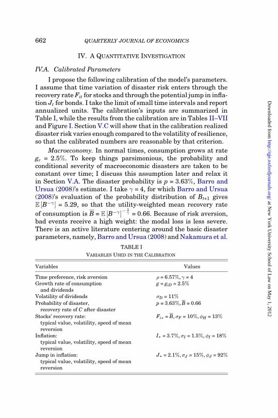
I propose the following calibration of the model’s parameters.I assume that time variation of disaster risk enters through therecoveryrateFit forstocks andthroughthepotential jumpininfla-tionJt forbonds. I takethelimit of small timeintervals andreportannualized units. The calibration’s inputs are summarized inTable I, while the results from the calibration are in Tables II–VIIandFigureI. SectionV.C will showthat inthecalibrationrealizeddisasterriskvaries enoughcomparedtothevolatilityofresilience,so that the calibrated numbers are reasonable by that criterion.
Macroeconomy. In normal times, consumption grows at rategc = 2.5%. To keep things parsimonious, the probability andconditional severity of macroeconomic disasters are taken to beconstant over time; I discuss this assumption later and relax itin Section V.A. The disaster probability is p = 3.63%, Barro andUrsua (2008)’s estimate. I take γ = 4, for which Barro and Ursua(2008)’s evaluation of the probability distribution of Bt+1 givesE [B−γ ] = 5.29, so that the utility-weighted mean recovery rate
of consumption is B = E [B−γ ]−1γ = 0.66. Because of risk aversion,
bad events receive a high weight: the modal loss is less severe.There is an active literature centering around the basic disasterparameters, namely, BarroandUrsua (2008)andNakamuraet al.
TABLE I
VARIABLES USED IN THE CALIBRATION
Variables Values
Time preference, risk aversion ρ = 6.57%, γ = 4Growth rate of consumption g = giD = 2.5%
and dividendsVolatility of dividends σD = 11%Probability of disaster, p = 3.63%, B = 0.66
recovery rate of C after disasterStocks’ recovery rate: Fi∗ = B,σF = 10%,φH = 13%
typical value, volatility, speed of meanreversion
Inflation: I∗ = 3.7%,σI = 1.5%,φI = 18%typical value, volatility, speed of meanreversion
Jump in inflation: J∗ = 2.1%,σJ = 15%,φJ = 92%typical value, volatility, speed of meanreversion
at New
York U
niversity School of Law
on May 1, 2012
http://qje.oxfordjournals.org/D
ownloaded from

VARIABLE RARE DISASTERS 663
TABLE II
SOME VARIABLES GENERATED BY THE CALIBRATION
Variables Values
Ramsey discount rate δ = 16.6%Risk-adjusted probability of disaster pE[B−γt+1 ] = 19.2%Stocks: effective discount rate δi = 5.0%,Stock resilience: typical value, Hi∗ = 9.0%, σH = 1.9%
volatilityStocks: equity premium, conditional 6.5%, 5.3%
on no disasters, uncond.Real short-term rate 1.0%Resilience of one nominal dollar H$ = 16.0%5-year nominal slope yt (5)− yt (1): 0.57%, 0.92%
mean and volatilityLong-run− short-run yield: κ = 2.6%
typical valueInflation parameters I∗∗ = 6.3%,ψI = 13%,ψJ = 90%Bond risk premium: volatility σπ = 2.9%
Notes. The main other objects generated by the model are in Tables III–VII and Figure I.
(2011) who find estimates consistent with the initial Barro (2006)numbers.
The key number is the risk-neutral probability of disasters,pE [B−γ ] = 19.2%. This high risk-neutral probability allows themodel tocalibrate a host of high risk premia. Following BarroandUrsua, I set the rate of time preference to match a risk-free rateof 1%, so in virtue of (12), the rate of time preference is ρ = 6.6%.
Stocks. I use a growth rate of dividends giD = gC, consistentwith the international evidence (Campbell 2003, Table III). Thevolatilityof thedividendis σD=11%, as inCampbell andCochrane(1999). The speed of mean reversion of resilience φH is the speedof mean reversion of the P/D ratio. It has been carefully exam-ined in two recent studies based on U.S. data. Lettau and vanNieuwerburgh (2008) findφH =9.4%. However, they findφH =26%whenallowingforastructural breakinthetimeseries, whichtheysuggest is warranted. Cochrane (2008) finds φH = 6.1% (std.err.4.7%). I take the mean of those three estimates, which leads toφH = 13%. Given these ingredients, a typical volatility σH = 1.9%helps match the volatility of stock returns.13
13. The Online Appendix details a specific volatility process for Hit, whichsatisfies the requirement that volatility vanishes at a lower bound, see note 9.
at New
York U
niversity School of Law
on May 1, 2012
http://qje.oxfordjournals.org/D
ownloaded from

664 QUARTERLY JOURNAL OF ECONOMICS
To specify the volatility of the recovery rate Fit, I specify thatit has a baseline value Fi∗=B andsupport Fit ∈ [Fmin, Fmax]= [0, 1].That is, if there is a disaster, dividends can do anything fromlosing all their value to losing no value at all. The process for Hit
then implies that the corresponding average volatility for Fit, theexpected recovery rate of stocks in a disaster, is 10%. This maybe considered a high volatility. Economically, it reflects the factthat it seems easy for stock market investors to alternatively feelextreme pessimism and optimism (e.g., during the large turningpoints around 1980, 2001, and 2008). In any case, this perceptionof the risk for Fit is not directly observable, so the calibrationdoes not appear to contradict any known fact about observablequantities.
The disaster model implies a high covariance of stock priceswithconsumptionduringdisasters. Is that trueempirically?First,it is clear that we need multicountry data, as, for instance, apurely U.S.-based sample would not represent the whole distri-bution of outcomes because it would contain too few disasters.Using such multicountry data, Ghosh and Julliard (2008) finda low importance of disasters. On the other hand, Barro (2009)report a high covariance between consumption and stock returnsduring a disaster, which warrants the basic disaster model. Themethodological debate, which involves missing observations—forinstance due to closed stock markets, price controls, the mea-surement of consumption, and the very definition of disasters—islikely to continue for years to come. My reading of Barro (2009)is that the covariance between consumption and stock returns,once we include disaster returns, is large enough to vindicate thedisaster model.
Inflation and Nominal Bonds. For simplicity and parsimony,I consider the case when inflation does not burst during disasters,F$,t+1 = 1. Bond and inflation data come from CRSP. Bond dataare monthly prices of zero-coupon bonds with maturities of one tofive years, from June 1952 through September 2007. In the sametime sample, I estimate the inflation process as follows. First, Ilinearize the LG process for inflation: It+1 − I∗ = e−φIΔt (It − I∗) +εI
t+1. Next, it is well known that inflation contains a substantialhigh-frequency and transitory component, which is in part due
Fortunately, many moments (e.g., stock prices) do not depend on the detalis ofthat process.
at New
York U
niversity School of Law
on May 1, 2012
http://qje.oxfordjournals.org/D
ownloaded from

VARIABLE RARE DISASTERS 665
to measurement error. The model accommodates this. Call It =It + ηt the measured inflation (which can be thought of as trendinflation plus mean-zero noise), while It is the trend inflation.I estimate inflation using the Kalman filter, with It+1 = C1 + C2It +εI
t+1 for the trendinflation and It =It +ηt for the noisy measurementof inflation. Estimation is at the quarterly frequency, and yieldsC2 = 0.954 (std.err. 0.020), that is, the speed of mean reversion ofinflation is φI = 0.18 in annualized values. Also, the annualizedvolatility of innovations in trend inflation is σI = 1.5%. I have alsochecked that estimating the process for It on the nominal shortrate yields substantially the same conclusion. Finally, I set I∗ atthe mean inflation, 3.7% (note that the slight nonlinearity in theLG term process makes I∗ differ from the mean of It by only atrivial amount).
To assess the process for Jt, I consider the five-year slope,st = yt (5) − yt (1). Equation (44) shows that, conditional on nodisasters, it follows (up to second-order terms) that st+1 = a +e−φJΔtst + bIt + εs
t+1, where Δt is the length of “a period” (e.g.,a quarter means Δt = 1
4). I estimate this process at a quarterlyfrequency. The coefficient on st is 0.78 (std.err. 0.043). This yieldsφJ = 0.92. The standard deviation of innovations to the slope is0.92%.
Tocalibrateκ, I considerthebaselinevalueof theyield, which
from (16) is yt (T)= yt (0)+κ+ ln1− 1−e−ψIT
ψIκ
T withψI =φI −2κ, and Icompute the value of κ such that it ensures yt (5)− yt (1)= 0.0057,the empirical mean of the five-year slope. This gives κ = 2.6%. By(9), this implies that in a disaster the expected jump in inflationis J∗ = 2.1%.
As a comparison, Barro and Ursua (2008) find a medianincrease of inflation during disasters of 2.4%. They find a medianinflation rate of 6.6% during disasters, compared to 4.2% forlong samples taken together. This is heartening, but one mustkeep in mind that Barro and Ursua (2008) find that the averageincreaseininflationduringdisasters is equal to109%—becauseofhyperinflations, inflation is very skewed.14 I conclude that a jump
14. Thereis adifferencebetweenwars andfinancial disasters: wars veryrarelylead to deflations, but financial disasters often do, especially during the GreatDepression. Theinflationjumpis a bit higherduringwars thanfinancial disasters,by about 1% or 4%, depending on whether one takes the median or the meanof winsorized values. It is useful to note that financial disasters in non-OECDcountries are typically inflationary.
at New
York U
niversity School of Law
on May 1, 2012
http://qje.oxfordjournals.org/D
ownloaded from

666 QUARTERLY JOURNAL OF ECONOMICS
in inflationof 2.1% is consistent withthehistorical experience. In-vestors do not know ex ante if disasters will bring about inflationor deflation; on average, however, they expect more inflation.
As there is considerable variation in the actual jump ininflation, there is much room for variations in the perceived jumpin inflation, Jt = J∗ + Jt—something that the calibration willindeed deliver. We saw that empirically the standard deviationof the innovations to the spread is 0.92% (in annualized values),whereas in the model it is (K5 − K1)σπ. Hence, we calibrate σπ =2.9%. As a result, the standard deviation of the five-year spreadis (K5−K1)σπ√
2φJ= 0.68%, while in the data it is 0.79%. Therefore, the
model is reasonable in terms of observables.An important nonobservable is the perceived jump in infla-
tion during a disaster, Jt. Its volatility is σJ = σπpE[B−γ ] = 15.4%, and
its population standard deviation is σJ√2φJ
= 11%. This is arguablyhigh, although it does not violate the constraint that the actualjump in inflation should be more dispersed than its expectation(see Section V.C). One explanation is that the yield spread hassome high-frequency transitory variation that leads to a veryhigh measurement of φJ; with a lower value one would obtaina considerably lower value of σJ. Another interpretation is thatthe demand for bonds shifts at a high frequency (perhaps forliquidityreasons). Whilethis is capturedbythemodel as a changein perceived inflation risk, it could be linked to other factors. Inany case, we shall see that the model does well in a series ofdimensions explored in Section IV.C.
Fixed Versus Variable pt The baseline calibration uses afixed pt. Let us see how things would change with a variable pt.If only pt varied, then the correlation between stock and bondrisk premia would be perfect. Empirically, we shall see that thecorrelation is much closer to 0, which suggests that asset-class-specificfactors drive the bulk of stock versus bond returns, ratherthan a common factor. This suggests that a calibration with aconstant pt is a useful first pass.
Tobe more quantitative, one wouldlike long time series of PtDt
and of real bond yields. To obtain such a long-term time series, Iuse the real short-term yield. Then, I regress Δ ln Pt
Dt=α+βΔrft +εt.
I observe that, in the model, pt affects rft and ln PtDt
, but that Fit
affects only PtDt
. Hence, using the model, the interpretation ofthe R2 is an answer to the question: how much of the variation
at New
York U
niversity School of Law
on May 1, 2012
http://qje.oxfordjournals.org/D
ownloaded from

VARIABLE RARE DISASTERS 667
in PtDt
comes from pt rather than Fit? Empirically, R2 = 13% andβ = −2.1 (std.err. 1.1). This means that, prima facie, 87% of thevariation in the P/D ratio comes from the recovery rate, and 13%from changes in pt. For the calibration’s parsimony, I take σp = 0.Using the regression on the Cochrane and Piazzesi (CP, 2005)factor, regressing Δ ln Pt
Dt= α + βΔCPt + εt, yields an R2 of 0.04%.
This also points to a very small role for a common shock in bondversus stock premia. I note that this 13% / 87% breakdown is, ofcourse, provisional. In addition, it is undoubtedly the case thatin some episodes, variations in pt are important (e.g., during the2008 crisis), and then it is useful topay the somewhat higher costof using the Epstein-Zin model developed later.
Let me expand on the theme that the correlation betweenstockandnominal bondpremiaappears tobesmall. Viceira(2007)reports that thecorrelationbetweenstockandbondreturns is 3%.The correlation between the change in the CP factor and stockmarket returns is 3%, and the correlation between the level of CPand the change in stock market returns is also 3%, at monthlyfrequencies. In the model, this could be accounted for by settingcorr
(εJ
t+1,−εHi,t+1
)' corr
(εJ
t+1, εDi,t+1
)' 3%.
On the Degree of Parsimony of this Calibration. This article ismainly concernedwith the value of stocks andgovernment bonds.It uses two latent measures of riskiness, one for real quantities(the stock resilience Hit) and another for nominal quantities (thebond risk premium πt), both of which load on just one macroshock, the disaster shock. This assumption of at least one riskpremium for nominal quantities and another risk premium forreal quantities is used by several authors, for example, Wachter(2006), Piazzesi and Schneider (2007), Bansal and Shaliastovich(2009), and Lettau and Wachter (2011).
My conclusion is that it is hardly possible to be more par-simonious and still account for the basic facts of asset prices.Indeed, a tempting, though ultimately inadequate, idea would bethe following: nominal bonds and stocks are driven by just onefactor, perhaps the disaster probability. However, there is muchevidence that risk premia are driven by more than one factor(see above, and also Fama and French 1993 who find that fivefactors are necessary to account for stocks and bonds). Hence, theframework in this article using twotime-varying risk premia (onefor nominal assets, one for real assets) is, in a sense, the minimalframework to make sense of asset price puzzles on stocks and
at New
York U
niversity School of Law
on May 1, 2012
http://qje.oxfordjournals.org/D
ownloaded from

668 QUARTERLY JOURNAL OF ECONOMICS
TABLE III
SOME STOCK MARKET MOMENTS
Data Model
Mean P/D 23 18.2Std. dev. lnP/D 0.33 0.30Std. dev. of stock returns 0.18 0.15
Notes. Stock market moments. The data are from Campbell (2003, Table 1 and 10)’s calculation for theUnited States 1891–1997.
nominal bonds. Of course, those premia ultimately compensatefor just one source of risk—disaster risk.
I next turn to the return predictability generated by themodel. Sometimes I use simulations, in a sample without disas-ters, as in most of the theory. The calibration was designed tomatch two-thirds of Table III, but the predictions in Figure I andTables IV–VII areout ofsample, that is, werenot directlytargetedin the calibration.
IV.B. Stocks: Level, Excess Volatility, Predictability
Average Levels. The equity premium (conditional on no dis-asters) is re
it − rf = pE [B−γ ] (1− Fi∗) = 6.5%. The unconditionalequity premium is 5.3% (the above value minus p (1− Fi∗)). So,as in Barro (2006), the excess returns of stocks mostly reflect arisk premium, not a peso problem.15 The mean value of the P/Dratio is 18.2 (and is close to equation (14), evaluated at Hit = 0), inline with the empirical evidence reportedin Table III. The centralvalue of the D/P ratio is δi = 5.0%. 16
“Excess” Volatility. The model generates “excess” volatility
and predictability. Consider (14), PitDit
=1+Hitδi+φHδi
. As stock market
resilience Hit is volatile, so are stock market prices and P/Dratios. Table III reports the numbers. The standard deviation ofln (P/D) is 0.27. Volatile resilience yields a volatility of the logof the P/D ratio equal to 10%. For parsimony’s sake, I assume
15. Note that this explanation for the equity premium is very different fromthe one proposed in Brown, Goetzmann, and Ross (1995), which centers aroundsurvivorship bias.
16. In those tables, the sample sometimes includes the Great Depression, butas shown by Campbell (2003), for the stock market moments considered, the broadfacts do not depend on including the Great Depression.
at New
York U
niversity School of Law
on May 1, 2012
http://qje.oxfordjournals.org/D
ownloaded from

VARIABLE RARE DISASTERS 669
that innovations to dividends and resilience are uncorrelated.The volatility of equity returns is 15%. I conclude that the modelcan quantitatively account for an “excess” volatility of stocksthrough a stochastic risk-adjusted severity of disasters. In ad-dition, changes in the P/D ratio reflect only changes in futurereturns, not future dividends. This is in line with the empiricalfindings of Campbell and Cochrane (1999).
Predictability. Consider (14) and (15). When Hit is high, (15)implies that the risk premium is low and P/D ratios (14) arehigh. Hence, themodel generates above-averagesubsequent stockmarket returns when the market-wide P/D ratiois belowaverage.This is the view held by many, but not all, researchers (see thediscussion in Cochrane 2008). The model predicts the followingmagnitudes for regression coefficients.
PROPOSITION 5. (Predictingstockreturns via D/Pratios) Considerthepredictiveregressions of thereturnfromholdingthestockfrom t to t + T, rit→t+T, on the initial dividend-price ratio,
ln(
DitPit
):
rit→t+T = αT + βT ln
(Dit
Pit
)
+ noise(26)
rit→t+T = α′T + β′T
(Dit
Pit
)
+ noise.(27)
In the model, for small holding horizons T, the slopes are, tothe leading order: βT = (δi + φH)T and β′T =
(1+φHδi
)T.
Proof. Proposition 1 states the expected returns over a shorthorizon T tobe re
it→t+T = (δ −Hit)T. Equation (14) implies that theright-hand side of (26) is, to the leading order, ln (D/P)t = ln δi −
Hitδi+φH
. Sotheregressionis, toa first order, reit→t+T =(δ−Hi∗−Hit)T=
αT − βTHitδi+φH
. Equating the Hit terms, βT = (δi + φH)T. The samereasoning yields β′T. �
The intuition for the value of βT is as follows. First, the slopeis proportional to T simply because returns over a horizon T areproportional to T. Second, when the P/D ratio is lower than thebaseline by 1%, it increases returns through two channels: thedividend yield is higher by δi%, and mean reversion of the P/Dratio creates capital gains of φ%.
Using the paper’s calibration of δi = 5% and φH = 13%, Propo-sition 5 predicts a slope coefficient β1 = 0.18 at a one-year horizon.
at New
York U
niversity School of Law
on May 1, 2012
http://qje.oxfordjournals.org/D
ownloaded from

670 QUARTERLY JOURNAL OF ECONOMICS
TABLE IV
PREDICTING RETURNS WITH THE DIVIDEND/PRICE RATIO
Data Model
Horizon Slope s.e. R2 Slope R2
1 yr 0.11 (0.053) 0.04 0.17 0.064 yr 0.42 (0.18) 0.12 0.45 0.198 yr 0.85 (0.20) 0.29 0.79 0.30
Notes. Predictive regression for the expected stock return rit→t+T = αT + βT ln
(DitPit
), at horizon
T (annual frequency), up to an 8-year horizon. The data are from Campbell (2003, Table 10 and 11B)’scalculation for the United States 1891–1997.
This prediction is in line with the careful estimates of Lettau andvan Nieuwerburgh (2008) who find a β1 value of 0.23 in theirpreferred specification. Also, Cochrane (2008) runs regression(27) at the annual horizon, and finds β′1 = 3.8 with a standarderror of 1.6. Proposition 5 predicts β
′
1 = 3.6. We note that theapproximation in Proposition 5, valid for “small” T, appears tobe valid up to approximately a one-year holding period. Table IVreports the model predictions for large T, using simulations, andtheir arguably good congruence with empirical data.
I conclude that the model is successful in matching not onlythe level but also the variation and predictability of the stockmarket.
Characteristics Versus Covariances. In a rare-disaster econ-omy, characteristics tend to predict returns better than covari-ances, which a strand of research argues is true (Daniel andTitman 1997). Indeed, in a sample without disasters, betas willonly reflect the covariance during “normal times,”but risk premiaare only due to the covariance with consumption in disasters.The two can be entirely different. Hence, the “normal-times”betas can have no relation with risk premia. However, “charac-teristics,” like the P/D ratio, imbed measures of risk premia (asin (14)). Hence, characteristics will predict returns better thancovariances.
However, there could be some spurious links if stocks withlow Hi∗ have higher cash-flow betas. One could conclude thata cash-flow beta commands a risk premium; however, this isnot because cash-flow betas cause the latter, but simply because
at New
York U
niversity School of Law
on May 1, 2012
http://qje.oxfordjournals.org/D
ownloaded from

VARIABLE RARE DISASTERS 671
stocks with high cash-flow betas happen to be stocks that have alarge loading on the disaster risk.
These points may help explain the somewhat contradictoryfindings in the debate about whether characteristics or covari-ances explain returns. When normal-times covariances badlymeasure the true risk, as is the case in a disaster model,characteristics will often predict expected returns better thancovariances.17
IV.C. Bond Premia and Yield Curve Puzzles
Excess Returns and Time-Varying Risk Premia.i. Bonds Carry a Time-Varying Risk Premium. Equation (18)
indicates that bond premia are (to a first order) proportional tobond maturity T. This is the finding of Cochrane and Piazzesi(2005). The explanatory factor here is the inflation premium πt,that is, compensation for a jumpin inflation if a disaster happens.The model delivers this because a bond’s loading of inflation riskis proportional to its maturity T.
ii. The Nominal Yield Curve Slopes Up On Average. Supposethat when a disaster happens, inflation jumps by J∗ > 0. Thisleads toa positive parametrizationκ of the bondpremia (equation(9)). The typical nominal short-term rate (i.e., the one correspond-ing toIt =I∗) is y (0)=δ−H$+I∗, while the long-term rate is y (0)+κ(i.e., − limT→∞ ln
Z$t(T)T ). Hence, the long-term rate exceeds the
short-term rate byκ > 0. The yieldcurve slopes up. Economically,this is because long-maturitybonds aremoresensitivetoinflationrisk than short-term bonds, so they command a risk premium.
On the other hand, in the model, the yield curve on realbonds is flat: all yields are equal to rf . The empirical evidence onreal bonds is scarce and mixed (e.g., Nakamura et al. 2011). Inthe UK, the real yield curve has been downward sloping, but inthe US, it has been upward-sloping. Hence, a flat real yield curvemay be a good benchmark.
The Forward Spread Predicts Bond Excess Returns. FamaandBliss (1987)regress short-termexcess bondreturns onthefor-ward spread, that is, the forward rate minus the short-term rate:
17. A recent working paper (Koijen, Lustig, and van Nieuwerburgh 2010)brings new substance to this debate, showing that value stocks’ dividends fell alot during the Great Depression.
at New
York U
niversity School of Law
on May 1, 2012
http://qje.oxfordjournals.org/D
ownloaded from

672 QUARTERLY JOURNAL OF ECONOMICS
Fama-Bliss regression: Excess return on bond of(28)
maturity T = αT + βT ∙ (ft (T)− rt) + noise.
The expectation hypothesis yields constant bond premia and,thus, predicts βT = 0. I next derive the model’s prediction.As in the calibration var(It)ψ
2I
var(πt)= 0.023, I highlight the case
where this quantity is small, which means that changes in theslope of the yield curve come from changes in the bond riskpremium rather than from changes in the drift of the short-termrate.
PROPOSITION 6. (Coefficient in the Fama-Bliss regression) Theslope coefficient βT of the Fama-Bliss regression (28) is givenin (45). When var(It)ψ
2I
var(πt)� 1,
(29) βT = 1 +ψJ
2T + O (T2) .
When var (πt) = 0 (no risk premium shocks), the expectationhypothesis holds and βT = 0. In all cases, the slope βT is non-negative and eventually goes to 0: limT→∞ βT = 0.
To understand the economics of the previous proposition,consider the variable part of the two sides of the Fama-Blissregression (28). The excess return on a T−maturity bond isapproximately Tπt (see equation (18)), while the forward spreadis ft (T)− rt ' Tπt (see equation (21)). Both sides are proportionalto πtT. Thus, the Fama-Bliss regression (28) has a slope equal to1, which is the leading term of (29).
This valueβT above1 is preciselywhat Fama andBliss (1987)have found, a result confirmed by Cochrane and Piazzesi (2005).This is quitehearteningforthemodel. Table V reports theresults.We also see that as maturity increases, coefficients initially risebut then fall at long horizons, as predicted by Proposition 6.Economically, most of the variations in the slope of the yieldcurveare due tovariations in the risk premium, not due tothe expectedchange of inflation.
The Slope of the Yield Curve Predicts Future Movements inLong Rates. Campbell andShiller (CS, 1991) findthat a highslopeof the yieldcurve predicts that future long-term rates will fall. CSregress yield changes on the spread between the yield and theshort-term rate:
at New
York U
niversity School of Law
on May 1, 2012
http://qje.oxfordjournals.org/D
ownloaded from

VARIABLE RARE DISASTERS 673
TABLE V
FAMA-BLISS EXCESS RETURN REGRESSION
Data Model
Maturity T β (std. err.) R2 β R2
2 yr 0.99 (0.33) 0.16 1.33 0.343 yr 1.35 (0.41) 0.17 1.71 0.234 yr 1.61 (0.48) 0.18 1.84 0.145 yr 1.27 (0.64) 0.09 1.69 0.08
Notes. The regressions are the excess returns on a zero-coupon bond of maturity T, regressed on thespread between the T forward rate and the short-term rate: rxt+1 (T) = α + β (ft (T)− ft (1)) + εt+1 (T).The unit of time is one year. The empirical results are from Cochrane and Piazzesi (2005, Table II). Theexpectation hypothesis implies β = 0.
TABLE VI
CAMPBELL-SHILLER YIELD CHANGE REGRESSION
Data Model
Maturity T β (std. err.) β
3 m −0.15 (0.28) −1.036 m −0.83 (0.44) −1.1612 m −1.43 (0.60) −1.4124 m −1.45 (1.00) −1.9248 m −2.27 (1.46) −2.83
Notes. The regressions are the change in bond yield on the slope of the yield curve: yt+1 (T − 1)− yt (T)
=α+ βT−1 (yt (T)− yt (1))+εt+1 (T) . The time unit is one month. The empirical results are from Campbell,
Lo, and MacKinlay (1997, Table 10.3). The expectation hypothesis implies β = 1.
Campbell-Shiller regression:yt+Δt (T −Δt)− yt (T)
Δt= a + βT ∙
yt (T)− yt (0)T
+ noise.(30)
The expectation hypothesis predicts βT = 1. However, CS findnegativeβT ’s, witharoughlyaffineshapeas afunctionofmaturity(see Table VI). This empirical result is predicted by the model, asthe next proposition shows. As in the calibration var(It)φ
2I
var(πt)= 0.045,
I highlight the case where these quantities are small.
PROPOSITION 7. (Coefficient in the Campbell-Shiller regression)The slope coefficient βT in the Campbell and Shiller (1991)regression (30) is given by (46). When φ2
I var(It)var(πt)
� 1, κT � 1,
βT =−(
1 + 2ψj−ψI
3 T)
+o (T)when T → 0, andβT =−ψJT +o (T)
when T � 1.
at New
York U
niversity School of Law
on May 1, 2012
http://qje.oxfordjournals.org/D
ownloaded from

674 QUARTERLY JOURNAL OF ECONOMICS
Table VI also contains simulation results of the model’spredictions. They are in line with CS’s results. To understandthe economics better, I use a Taylor expansion in the case whereinflation is minimal. The slope of the yield curve is, to the leadingorder, yt(T)−yt(0)
T = πt2 + O (T). Hence, toa first-order approximation
(when inflation changes are not very predictable), the slope of theyield curve reflects the bond risk premium. The change in yield is(the proof of Proposition 7 justifies this):
yt+Δt (T −Δt)− yt (T)Δt
' −∂yt (T)∂T
=−πt
2+ O (T) .
Hence, the CS regression yields a coefficient of −1, to the leadingorder. Economically, it means that ahighbondpremiumincreasesthe slope of the yield curve (by πt
2 ).As bond maturity increases, Proposition 7 predicts that the
coefficient in the CS regression becomes more and more negative.The economic reason is the following. For long maturities, yieldshave vanishing sensitivity to the risk premium, which the modelsays has the shape yt (T) = a + bπt
T + o(
1T
)for some constants a, b.
Thus, the slope of the yieldcurve varies with bπtT2 , andthe expected
change in the yieldis −bφJπtT . Sothe slope in the CS regression (30)
is βT ' −φJT. Ontheotherhand, theexpressionforβT shows thatwhen the predictability due to inflation is non-negligible, the CScoefficient should go to 1 for very large maturities.
In Table VI, we see that the fit between theory and evidenceis rather good. The only poor fit is for a short maturity. TheCS coefficient is closer to 0 than in the model. The short-termrate has a larger predictable component at short-term horizonsthan in the model. For instance, this could reflect a short-termforecastability in Fed Funds rate changes. That feature could beadded to the model, as in the Online Appendix. Given the smallerrors in fit, it is arguably better not tochange the baseline modelwhich broadly accounts for the CS finding. Economically, the CSfinding reflects the existence of a stochastic one-factor bond riskpremium.
A Tent-shaped Combination of Forward Rates Predicts theBond Risk Premium. Cochrane and Piazzesi (CP, 2005) establishthat (i) a parsimonious description of bond premia is given by astochasticone-factorriskpremium, (ii) (zero-coupon) bondpremiaare proportional to bond maturity, (iii) this risk premium is
at New
York U
niversity School of Law
on May 1, 2012
http://qje.oxfordjournals.org/D
ownloaded from

VARIABLE RARE DISASTERS 675
empirically well approximatedby a “tent-shaped” linear combina-tion of forward rates, and (iv) a regression of excess bond returnson five forward rates gives such a tent shape.
Equation (18) is consistent with their findings (i)–(ii): there isa single bondrisk factorπt, andthe loading on it is proportional tobondmaturity.18 Economically, this is because a bondof maturityT has a sensitivity to inflation risk approximately proportionalto T.
We shall see that the model delivers finding (iii) but notfinding (iv). It cannot deliver (iv) because it has only two factors,so that five forwards rates in a regression would be collinear. Itis conceivable that richer extensions (e.g., with five factors) of themodel might deliver (iv), although at the same time it would benice to see if (iv) replicates robustly in other countries (see Kozak2011).
However, we shall see that the model is account for CP’sfinding (iii). To understand this, rewrite (21) as:
ft (T) = F (T) + e−ψITIt + Λ (T)πt, Λ (T) ≡e−ψIT − e−ψJT
ψJ − ψI.
This model’s interpretation of the CP “tent-shaped” effect is that,inthemodel, forwardrates of maturity T necessarilyhavea “tent-shaped” loading Λ (T) on the bond risk premium. To see that themodel’s loadingΛ (T) is tent-shaped, observe that Λ (0)=Λ (∞)=0andΛ (T) > 0 for T > 0. We saw earlier (after Lemma 2) that theeconomic reason for this tent shape of Λ (T) is that short-termbonds have no inflation risk premium, and long-term forwardsare constant (in this model, ft (∞) = δ − H$ + I∗∗), so that onlyintermediate maturity forwards have a loading on the bond riskpremium.
To econometrically capture the bond risk premium, a tent-shaped
∑5T=1 wTft (T) combination of forwards predicts the bond
risk premium. The simple (∑5
T=1 wT) and maturity-weighted(∑5
T=1 TwT) sums oftheweights shouldberoughly0, soas toelimi-nateslow-movingfactors suchas e−ψITIt uptosecond-orderterms.This reasoning leads one toask if there is a simple combination of
18. This is not an artifact of postulating a single bond risk premium, comingfromJt. If thereareK bondriskpremia Jkt, withdifferent speeds ofmeanreversion(as inthemultifactormodel of theOnlineAppendix), then, totheleadingorder, therisk premium on a bond of maturity T is still Tπt, with πt = ptEt
[B−γt+1
]∑Kk=1 Jkt.
at New
York U
niversity School of Law
on May 1, 2012
http://qje.oxfordjournals.org/D
ownloaded from

676 QUARTERLY JOURNAL OF ECONOMICS
forward rates that one might expect to robustly proxy for the riskpremia. The next proposition provides an answer.19
PROPOSITION 8. (Estimation-free combinations of forwards toproxy for the bond risk premium) Given time horizons a andb, consider the following “estimation-free” combinations offorwards:
(31) CPEFt (a, b) ≡
−ft (a) + 2ft (a + b)− ft (a + 2b)b2
,
where ft (T) are the forwards of maturity T. Then, uptothird-order terms, for small a and b, CPEF
t (a, b) = (ψI + ψJ)πt isproportional to the bond risk premium.
Proof. From (21), up tothird-order terms, CPEFt = (ψI + ψJ)πt. The
leading inflation term is −ψ2I It, a third-order term. �
For instance, CPEFt (1, 2) = −ft(1)+2ft(3)−ft(5)
4 uses the forwardsup to a maturity of 5 years. Proposition 8 suggests that CPEF
tcouldbeusedinpracticetoproxyforthebondriskpremia withoutrequiringa preliminaryestimation.20 Overtheperiod1964–2008,repeating the CP analysis gives an average R2 of 28% to predictexcess bond return, while the estimation-free CPEF
t (1, 2) yieldsa R2 of 23%. This is arguably a good performance, given the CPanalysis uses five regressors, and the estimation-free CPEF
t usesjust one. In addition, the correlation between CP’s variable andCPEF
t is 0.89. Finally, consider a country with a short data set:the estimate of the CP coefficients will be very noisy. Researcherscould thus use the estimation-free CPEF
t to evaluate risk premia.I conclude that the model can account for the CP findings
(i)–(iii) and proposes new combinations of factors to predict thebond risk premium. The latter are “estimation-free” and might beuseful empirically.
19. Combination (31) is not unique in the present two-factor model. However,if we add a small third persistent factor, then the combination becomes unique. Itgoes to (31) when the extra persistence of that factor and inflation go to 0 (seethe Online Appendix). In that sense, (31) is a special combination that comesnaturally out of a small perturbation of the baseline model. Lettau and Wachter(2011) proposed earlier another combination of theoretical factors to obtain therisk premium, but it is not estimation-free.
20. The CP estimate is very close to 8CPEFt (1, 2) − 1
2 CPEFt (2, 1), which
is−2f (1) + 0.5f (2) + 3f (3) + 0.5f (4)− 2f (5).
at New
York U
niversity School of Law
on May 1, 2012
http://qje.oxfordjournals.org/D
ownloaded from

VARIABLE RARE DISASTERS 677
FIGURE IOption implied volatility in the model and in the data.
This figure presents the Black-Scholes annualized implied volatility of aone-month put on the stock market. The solid line is from the model’s calibration.The dots are the empirical average (January 2001 to February 2006) for theoptions on the S&P 500 index (Figlewski 2008). The initial value of the marketis normalized to 1. The implied volatility of deep out-of-the-money puts is higherthan the implied volatility of at-the-money uts, which reflects the probability ofrare disasters.
IV.D. Options
I now investigate whether the model’s calibration (whichdid not target any option-specific value) yields good values foroptions. I calculate the model’s Black-Scholes implied volatilitiesof puts with a one-month maturity. I am very grateful to StephenFiglewski for providing the empirical implied volatilities of one-month options on the S&P 500 from January 2001 to February2006 (Figlewski 2008).
Figure I reports the impliedvolatilities from the data andthecalibration. Thecorrespondenceis quitegood, despitethefact thatno extra parameter was tuned to match option prices.21 Hence,I conclude that as a first pass and for the maturity presentedhere, the variable rare disasters model can yield correct optionprices. Du (2011) finds other parametrizations of jumps thatmatch option prices. Of course, a more systematic study wouldbe desirable. Farhi et al. (2009) investigate the link between
21. I useσ = 15% (from Table III), and the central case Fi,t+1 = F∗, which yieldsHit = Hi∗.
at New
York U
niversity School of Law
on May 1, 2012
http://qje.oxfordjournals.org/D
ownloaded from

678 QUARTERLY JOURNAL OF ECONOMICS
currency option prices andcurrency levels, finding support for theexistence of a disaster risk premium.
Backus, Chernov, and Martin (forthcoming) study a specifi-cation that equity dividends are Dt = Cλt for some λ > 0, andcannot fit option prices in a disaster framework with constantdisaster risk. In their framework, a high λ (about 4) is necessaryto attain a high volatility of equity (so that dividend volatility isλ times consumption volatility). But then, equity is immenselyrisky during disasters, and put prices are too high. In contrast,in the present framework, equity volatility comes from resiliencevolatility, andput prices can be moderate andcalibrate naturally.
Proposition 3 suggests a way toextract key structural param-eters of disasters fromoptions data. Stocks witha higherput price(controlling for “normal-times” volatility) should have a higherrisk premium, because they have higher future expected returns.Evaluating this prediction would be most interesting. Supportiveevidence comes from Bollerslev, Tauchen, and Zhou (BTZ, 2009).They findthat when put prices are high, subsequent stock marketreturns are high. This is qualitatively what a disaster-basedmodel predicts.
For a more quantitative assessment, consider the “variancepremium” VPt, which is the risk-neutral expected variance mi-nus the expected variance (conditional on no disasters). It isstraightforward to derive VPt = ptED
[B−γt+1 (1− Fi,t+1)
2], as thejump size in a disaster is 1 − Fi,t+1. BTZ regress annualizedstock market returns on the variance premium VPt. Table VIIreports the results.22 In addition, the mean and standard de-viation of VPt are, respectively, 2.2% and 0.53% in the BTZdata, and 3.4% and 0.66% in the model. Hence, the model isbroadly congruent with the empirical results of BTZ. It cannotaccount for all the patterns in the variance premium, as it isa one-factor model and the VIX index clearly exhibits somehigh-frequency transient dynamics. They might be accounted forby a resilience made of fast and slow components, as in theOnline Appendix. Still, it is comforting to see that the modelcan generate some of the qualitative and quantitative empiricalpatterns.
22. I convert BTZ’s results to annualized units, which multiplies their slopesby 100
12 . The model’s baseline prediction (i.e., neglecting small nonlinear terms)
for the slope in Table VII is β = −(∂Hit∂Fit
)/(∂VPt∂Fit
)= 1(2(1−F∗))
= 1.5. Table VII’ssimulations confirm the prediction.
at New
York U
niversity School of Law
on May 1, 2012
http://qje.oxfordjournals.org/D
ownloaded from

VARIABLE RARE DISASTERS 679
TABLE VII
PREDICTING RETURNS WITH THE VARIANCE PREMIUM
Data Model
Horizon Slope std. err. R2 Slope R2
1 m 3.2 (1.8) 0.01 1.6 0.0063 m 3.9 (1.4) 0.06 1.6 0.026 m 2.5 (1.2) 0.05 1.6 0.0312 m 1.0 (0.9) 0.01 1.4 0.05
Notes. Predictive regression for the expected stock return 1T rit→t+T = αT + βTVPT at horizon T (using
annualized units). VPT is the variance risk premium. The empirical data come from Bollerslev, Tauchen,and Zhou (2009, Table II).
IV.E. Corporate Bonds
The calibration allows us to evaluate Proposition 4. Thedisaster risk premium is πD
i = yi − yG − λi, the difference betweenthe yield on corporate bonds and governance bonds minus thehistorical default rate of corporate bonds. The rare disaster modelprovides a macroeconomic foundation for Almeida and Philip-pon (2007)’s view that the corporate spread reflects the exis-tence of bad states of the world and for reduced-form models ofcredit risk.
Almeida and Philippon (2007) yield an estimate of πDi as the
difference between the risk-adjusted annualized probability ofdefault andthehistorical one.23 Forinstance, this implies πD
i tobeabout 4.05% fora bondratedB (resp. 0.60% fora AAA bond). WithpE [B−γ ]=19.2%, this means that the expectedloss in a disaster is4.05%0.192 =21% (resp. 0.60%
0.192 =3.2% for a AAA bond). This is a moderateloss. We see how easily, though, a disaster model can rationalizethe corporate spread.
Moody’s (1999) reports evidence on the United States. Dur-ing the Great Depression, the realized loss rate was 5.3% on“investment-grade” bonds (of which AAA are the least risky) and25% for the “speculative-grade” bonds (a category that comprises
23. I take Almeida and Philippon (2007)’s Table III, which has the 10-yearrisk-neutral and historical probability, and apply the transformation− ln (1−x)
10 toobtain the annualized probability of default. I also add back the AAA-Treasuryspread of 0.51% to get the actual AAA-Treasury spread. This yields the followingdisaster premia: 0.60% (AAA bonds), 1.11% (AA), 1.71% (A), 2.57% (BBB), 3.06%(BB), and 4.05% (B). Almeida and Philippon (2007) do not report standard errors.
at New
York U
niversity School of Law
on May 1, 2012
http://qje.oxfordjournals.org/D
ownloaded from

680 QUARTERLY JOURNAL OF ECONOMICS
B bonds).24 This is roughly in line with the magnitude frommarket prices and disaster models.
Prediction(i) of Proposition 4 seems quitenovel. Theintuitionis the following. To take an extreme example, suppose agentsknow that there will be hyperinflation in disasters, so that thereal value of all nominal assets will be zero (F$ = 0). Then,government bonds lose all their advantage over corporate bonds,as the value of all bonds will be wiped out in a disaster. Hence,before the disaster, there should be no difference in the disasterrisk premium between government bonds, AAA bonds, or anynominal bond. In less extreme scenarios, the same logic applies:high inflation risk lowers the spread between nominal bonds,because high inflation compresses the performance of all nominalbonds in the disaster state.
Prediction(i) provides anexplanationfor KrishnamurthyandVissing-Jorgensen (2008)’s finding that when the Debt/GDP ratiois high, the AAA-Treasury and the BAA-AAA spreads are low:in their 1925–2005 U.S. sample, regressing the AAA-Treasuryand BAA-AAA spreads on the Debt/GDP ratio yields significantcoefficients of−1.5 and−1.2, respectively. The first AAA-Treasuryfinding can be explained by their favored interpretation of aliquidity demand for treasuries, but the BAA-AAA spread may beharder to explain by liquidity. The disaster hypothesis offers anexplanation for both, hence it is complementary to the liquidityexplanation. When Debt/GDP is high, the temptation to defaultvia inflation (should a risk occur) is high,25 thus F$ is low and soare nominal spreads.
Prediction (ii) of Proposition 4 allows one to think about theimpact of the government Debt/GDP ratio. It is plausible that ifthe Debt/GDP ratio is high, then—once there is a disaster—thegovernment will sacrifice monetary rectitude, so that Jt is high(this effect could be microfounded). This implies that when theDebt/GDP ratio (or the deficit/GDP) is high, then long-term ratesare high and the slope of the yield curve is steep (controllingfor inflation and expectations about future inflation in normaltimes). In addition, in the Krishnamurthy and Vissing-Jorgensen(2008) data, regressing bond rates minus the bill rate on the
24. I average over the twomethodologies in the Moody’s (1999) paper (Exhibits5-11 and 5-13). I use the 1932–1935 cumulative rate. The earlier losses are muchsmaller.
25. Catao and Terrones (2005) find that high Debt/GDP leads, on average, toan increase in inflation.
at New
York U
niversity School of Law
on May 1, 2012
http://qje.oxfordjournals.org/D
ownloaded from

VARIABLE RARE DISASTERS 681
Debt/GDP ratio yields a significant coefficient of 1.8, consistentwith the disaster hypothesis: when the Debt/GDP ratio is high,the bond risk premium is high, so the slope of the yield curve isalso high.
Likewise, suppose that an independent central bank hasa more credible commitment not to increase inflation duringdisasters (Jt smaller). Then, real long-term rates (e.g., nominalrates minus expected inflation) are lower and the yield curveis less steep. This effect works in an economy where Ricardianequivalence holds. Higher deficits increase long-term rates notbecause they “crowd out” investment but instead because theyincrease the government’s temptation to inflate away the debtif there is a disaster. In such a case, there is an inflation riskpremium on nominal bonds.
V. DISCUSSION AND EXTENSIONS
V.A. Epstein-Zin Preferences
As mentioned, the power utility model has one qualitativedeficiency: if the disaster probability increases, the risk-free ratedecreases so much that the prices of most assets, including aconsumption claim, go up.26 To remedy this strong movement oftherisk-freerate, I extendthemodel tothepreferences introducedby Epstein andZin (EZ, 1989), which allowone todecouple the in-tertemporal elasticity of substitution (IES), ψ, and risk aversion,γ.27 This decoupling is indexed byχ= 1−1/ψ
1−γ , which is equal to1 inthe case of power utility preferences.28 EZ show that the stochas-
tic discount factor (SDF) evolves as Mt+1Mt
= e−ρχ
(Ct+1Ct
)− 1χψ
R1/χ−1c,t+1 ,
where Rc,t+1 = Pc,t+1Pct−Ct
is the gross return of a consumption claim —
26. The same anomalous effect works with a change in the recovery rate ofconsumption, Bt+1, and is fixed by Epstein-Zin preferences.
27. This effect of “badnews increasetheprice”is alsopresent without anyrisk.In that case, the interest rate is rf = ρ + gC
ψ, and the stock price is Pt = Dt
ρ+gC/ψ−gD
by the Gordon formula. Hence, if both gC and gD go down by the same amount(bad news), the asset price increases, unless ψ > 1. That is why it is useful tohaveψ > 1. At the same time, we need γ > 1 to have large risk premia. EZ preferencesallowforψ > 1 andγ > 1, whereas powerutility preferences, which imposeψγ=1,do not.
28. This subsection complements the prior and different Epstein-Zin modelof Wachter (2009), whose many results require a unit IES, and the numericaltreatment in Gourio (2008a, 2008b).
at New
York U
niversity School of Law
on May 1, 2012
http://qje.oxfordjournals.org/D
ownloaded from

682 QUARTERLY JOURNAL OF ECONOMICS
the asset that gives a consumption Ct as a dividend and the priceof which we call PCt.
The Appendix presents a setup in which this Epstein-Zinmodel is exactly solved. To make the exposition more trans-parent, I present here the economics of the model using afirst-order approximation (in the exposition I neglect quadraticterms).29
The resilience of a consumption claim, Hct = ptE[B1−γ
t+1 − 1],
is again assumed to follow the LG-twisted process, Hc,t+1 =1+Hc∗1+Hct
e−φH Hc,t+εHc,t+1 totheleadingorder. Themaintool is thevalue
of the SDF.
THEOREM 3. (SDF with EZ preferences) In the Epstein-Zin setup,the stochastic discount factor is given exactly by (37) andapproximately by:
Mt+1
Mt= e−δ
(1 + (χ− 1)Hct + εM
t+1
)
×
{1 if there is no disaster at t + 1B−γt+1 if there is a disaster at t + 1
,(32)
where δ = ρ + gc/ψ, δc = δ − gc − χHc∗ and εMt+1 =
(1− χ) εHc,t+1
δc+φH. To the leading order, the risk-free rate is rft =
δ − ptEDt
[B−γt+1 (1 + (χ− 1)Bt+1)− χ
].
The key impact of disaster is in B−γt+1, as in the power utilitycase. However, it is nowmodulatedby the Hct term, which cancelsout in the power utility case, χ = 1. When χ decreases (up to apoint), the interest rate becomes less sensitive to pt, as people areless willing to increase savings when disaster risk is high.
Considera stock i. I defineits Epstein–Zin–enriched resiliencein (38), whose leading term is HEZ
it = Hit + (χ− 1)Hct, that is,
(33) HEZit = ptE
Dt
[B−γt+1 (Fi,t+1 + (χ− 1)Bt+1)− χ
].
When χ = 1, (33) is the earlier definition of resilience, givenin (4). The EZ resilience is the power utility resilience plus anasset-independent term that reflects variation in the risk-freerate. Hence, when noise is small, introducing EZ preferenceschanges therisk-freeratebut leaves riskpremia unchangedtothe
29. TheOnlineAppendixfinds that, forparameters usedinthecalibration, thesecond-order terms are very small (less than 1% of the first-order terms).
at New
York U
niversity School of Law
on May 1, 2012
http://qje.oxfordjournals.org/D
ownloaded from

VARIABLE RARE DISASTERS 683
leading order (the risk premium remains ptEDt
[B−γt+1 (1− Fit)
]).30
This echoes Barro (2009), which find this result (EZ changes theinterest rate, but not the risk premium) when disaster risk isconstant over time, but finds it for a time-varying disaster risk.
I assume that the EZ-enriched resilience follows, up tosecond-order terms, an LG process, with HEZ
it = HEZi∗ + HEZ
it and
Et
[HEZ
i,t+1
]= 1+HEZ
i∗
1+HEZit
e−φH HEZit (to the leading order; see (40) for all
specifics). The next proposition shows that the above results onstocks (e.g., Theorem 1, Proposition 1) follow, provided one usesthe enriched notion of resilience.
PROPOSITION 9. (Stock price with EZ preferences) With EZ pref-erences, the price of a stock i is the same exact expression(14) as in the power utility case, but with the EZ-enrichedresilience:
(34)Pit
Dit=
1δi
(
1 +HEZ
it
δi + φH
)
, δi ≡ δ − gi −HEZi∗ .
In particular, a consumption claim has a resilience HEZCt =
χptEDt
[B1−γ
t+1 − 1], and its price is Pt = Ct
δc
(1 + χHCt
δc+φc
). We see that
in the case χ < 0 (i.e., an IES > 1 and γ > 1), when pt goes up,the resilience of a consumption claim and its price go down. Thisis the key qualitative effect from an EZ model. In contrast, thepower utility model (χ = 1) would lead to the opposite prediction,which is likely anomalous.
Consider now a more general stock. When χ < 0, as thedisasterprobabilitygoes up, thestockpricegoes down. This is trueas long as Fit ≤ Bt, that is, the asset is riskier than consumption.However, if the asset is very safe (e.g., with Fi,t+1 =1) andχ is neg-ative enough, then if the disaster probability goes up, the asset’sresilience and price go up. This corresponds to a “flight to safety.”
Calibration. I follow Barro (2009) and take ψ = 2. This leadsto a value χ = − 1
6 . For σp, I observe that the variations in therisk-free rate are small (Campbell and Cochrane 1995 calibratea constant risk-free rate), so I calibrate a small volatility of pt,
30. Comovement between the SDF and resilience also affects the asset’s riskpremium, which is −covt
(Mt+1Mt
, ri,t+1
). The Appendix derives terms due to the
normal-times covariance with the innovations in the SDF, but we shall see thatthey are quantitatively small.
at New
York U
niversity School of Law
on May 1, 2012
http://qje.oxfordjournals.org/D
ownloaded from

684 QUARTERLY JOURNAL OF ECONOMICS
σp = 0.4%, which implies a volatility of the risk-free rate of σr =0.55%. Tolower the number of free parameters, I assume that themovements in pt andFit areuncorrelated, andpreservethevaluesof all parameters as in the power utility calibration in Table I,except the rate of time preference, which changes to ρ = 4.8%.Further details are in the Online Appendix.
It turns out that theextravolatilitycomingfromthevariationin pt increases the volatility of resilience only by a fraction 1%:σEZ
H = σH ∙ 1.01. To see why, consider the case of Fi,t+1 = Bt+1 = B.
Then, to the leading order, HEZit = χB
1−γpt + p∗B
−γFit. As χ is
small, theresilienceis not toosensitivetodeviationof thedisasterprobability from trend, pt, but it remains equally sensitive as inthe power utility case to the deviation of the recovery rate fromtrend, Fit. At least in this calibration, most of the volatility comesfrom the movement in the recovery rate, and most of the riskpremia come from disaster risk (the “normal-times” volatility inthe SDF is very small, σεM = 6.4%).
Hence, a time-varying probability usually has little impacton the volatility of stocks andtheir price-earnings ratio. However,themajorimpact of that probabilitylikelyoccurs intimes ofcrises,that is, when it suddenly moves a lot. During such episodes, thefraction of the variance explained by pt would be high.
Fornominal bonds withEpstein-Zinutility, wecananticipatethat the economics would be like in the power utility case, exceptfor an extra variation in the risk-free rate, in a fashion veryanalogous to the one developed in Proposition 13 of the OnlineAppendix.
The present EZ model has some limitations. Indeed, Naka-mura et al. (2011) find that empirically consumption drops acouple of years after the disaster strikes andthen partly recovers.Then, usinga numerical solution, theauthors findthat theimpactof EZ preferences on risk premia is first order, and the partial re-covery affects the relative premia of short-term versus long-termassets. The present setup, which assumes that consumption fallson impact and does not recover, misses that effect. I conjecturethat the present setupcouldbe extendedsoas toyieldpredictableconsumption dynamics after the disaster and complement theavailable numerical treatments, and then account for some fur-ther asset pricing puzzles (e.g., for short-term versus long-termassets). Still, thebenchmarkof consumptiondroppingat theonsetof the disaster is surely useful to study asset prices before the
at New
York U
niversity School of Law
on May 1, 2012
http://qje.oxfordjournals.org/D
ownloaded from

VARIABLE RARE DISASTERS 685
disaster, and the present model offers a reasonably transparentway (via equations (33) and (34)) to understand the economics ofthat benchmark.
To conclude, the main advantage of this Epstein-Zin settingis that it inverts the anomalous qualitative impact of pt. At thesame time, the quantitative impact of the Epstein-Zin settingis not very large on average, though it can be large in times ofcrises. Hence, I recommend using the power utility setting withtime-varying recovery rates for a host of asset pricing issues (e.g.,excess volatility, predictability, options, and the impact of pt onthe relative risk premia) and paying the cost of the somewhatmore complex Epstein-Zin framework only when movements inpt affect the risk-free rate too much. A simple way to think aboutall these issues is to use the Epstein-Zin enriched resilience (33),which incorporates much of the economics in a compact way.
V.B. Alternative Interpretation of the Model
Some derivations on stocks andbonds donot dependsolely onthe disaster hypothesis. On the other hand, for some predictionsabout “tail assets” (e.g., options and high-grade corporate bonds)the disaster model is crucial. This is formalized in the nextproposition.
PROPOSITION 10. (Models generating the same stock and govern-ment bond prices as a disaster economy, but not the sameoption and corporate bond prices) Consider a model withstochasticdiscount factor Mt+1
Mt=e−rf
(1 + εM
t+1
)anda stock with
dividend following Di,t+1Dit
= egiD(1 + εD
i,t+1
), where all εH
i,t+1’s have
expected value 0 at time t. Call Hit = Et[εM
t+1εDi,t+1
]= Hi∗ +
Hi,t+1, so that −Hit is the risk premium on the dividend,and assume Hi,t+1 = 1+Hi∗
1+Hite−φH Hit + εH
i,t+1, with εHi,t+1 uncor-
related with the innovations to Mt+1Di,t+1(MtDit)
. Then, Theorem 1and Proposition 1 hold, except that the equity premium is−Hit and the interest rate is rf . Furthermore, suppose that
inflation is It = I∗ + It and follows It+1 = 1−I∗1−It
(e−φI It + εI
t+1
).
Call Et[εM
t+1εIt+1
]= π∗ + πt, the inflation risk premium, and
assume πt+1 = 1−I∗1−It
e−φJπt + επt+1, withEt[εM
t+1επt+1
]= 0. Also, use
the notationπ∗= (1− I∗)κ(1− e−φI − κ
). Then, Theorem 2 on
bond values (with H$ = 0) and Propositions 2, 6–8 on bondpredictability hold (except equation (19)).
at New
York U
niversity School of Law
on May 1, 2012
http://qje.oxfordjournals.org/D
ownloaded from

686 QUARTERLY JOURNAL OF ECONOMICS
However, sucha model genericallyhas different prices foroptions and corporate bonds (which are more tail-sensitive).
Proof. With Qt+1Qt
= 1 − It, MtDit
(1, Hit
)and MtQt
(1, It
1−I∗, πt
1−I∗
)
are both LG processes with the same moments as in the disastereconomy. �
Proposition 10 shows that in many models stocks and bondswill behave exactly as in a disaster economy (however, optionsor defaultable bonds will behave differently), so that disasteranalytics shed light on many models. Rather than a disaster-based pricing kernel, the proposition studies a generic pricingkernel Mt, which could include a “behavioral” one. Relatedly,in some respects one way to model “time-varying sentiment” ina time-consistent way would be to model it as a time-varyingperception of disaster risk. Note that it is hard for agents to learna “rational” perception of disaster risk, as feedback will be scant(Chen, Joslin, and Tran 2011).
Yet disaster models make clearly distinctive predictionsfor tail-sensitive assets such as options and high-grade cor-porate bonds (and gold, which could be modeled similarlyto a stock, but with a very high resilience). These assetsare naturally the object of scrutiny of the growing literaturethat examines disaster risk empirically, and to which I nowturn.
V.C. A Further Provisional Empirical Assessment
This sectionprovides anassessment of theempirical evidenceon the link between disasters and asset price movements, asworked out in the present model.
Are the Movements of Asset Prices Correlated with the Move-ments in Objective Disaster Risk?
i. Political Measures of Disaster Risk. A question very highon the empirical agenda is tofind “objective” measures of disasterrisk that ideally do not come from asset prices. A few papersattempt to do this. Using a database of 447 major internationalpolitical crises during the period 1918–2006, Berkman, Jacobsen,and Lee (2011) show that high war risk leads to a drop in assetprices: returns are low when a crisis starts and are high whenit ends, and crisis risk is positively correlated with the dividendyield. Other papers measure (on shorter data sets) the impact ofthe probability of war on asset prices. Bittlingmayer (1998) finds
at New
York U
niversity School of Law
on May 1, 2012
http://qje.oxfordjournals.org/D
ownloaded from

VARIABLE RARE DISASTERS 687
that political risk was an important factor of volatility between1880 and World War II. Amihud and Wohl (2004) document thelinkbetweentheprobabilityofthesecondIraqWar(obtainedfromprediction markets) and the stock market. All in all, a growingnumber of studies document a link between political risk and thevolatility and level of asset prices, in a way consistent with thedisaster hypothesis. A fully structural empirical analysis has yettobe carriedout, probably enrichedwith newdata, but the extantevidence is encouraging.
ii. Disaster Risk Measured by Tail Behavior of Asset Prices.Alternatively, we may detect disaster risk in asset prices. Boller-slev, Tauchen, and Zhou (2009) show that when put prices arehigh, future stock returns are low, like in this article. In addition,the high price of put prices is consistent with disaster risk. Boller-slev and Todorov (forthcoming) find large jumps in option pricesthat are much harder todetect than in the physical probability. Incurrency markets, Farhi et al. (2009) find that when put prices oncurrencies are high, the return on investing in “risky” currencies(by the measure of their put prices) is high. They find that when acurrency falls in value, its put prices increase, with a correlationof −0.4. This is consistent with the disaster view. Burnside et al.(2011) also calibrate that disaster risk might account for theviolations of uncovered interest rate parity.
In conclusion, put prices are high and they predict futurereturns, as in the disaster hypothesis. Hence, the evidence is,though not systematically so, supportive of the disaster hypoth-esis. Finally, a recent paper by Kelly (2011) finds that a movingaverage of the cross-sectional tail distribution of realized stockreturns may be a good proxy for aggregate tail risk, predictingequity returns.
Do High-yield Assets do Particularly Poorly During Disas-ters? Barro (2009) find that stocks indeed do particularly poorlyduring disasters. Farhi et al. (2009) report that high-yield cur-rencies do particularly poorly during currency market crashes,consistent with rare-event risk premia. Koijen, Lustig, and vanNieuwerburgh (2010) find that during the Great Depression div-idends of value stocks fell a lot more than dividends of growthstocks.31 Ongoing work with Joachim Voth investigates Russia
31. It also finds that the Cochrane and Piazzesi (2005) factor helps predictvalue stock returns. This might indicate that disaster risk is important for valuestocks and is higher in the cross-section of stocks when it is higher in the
at New
York U
niversity School of Law
on May 1, 2012
http://qje.oxfordjournals.org/D
ownloaded from
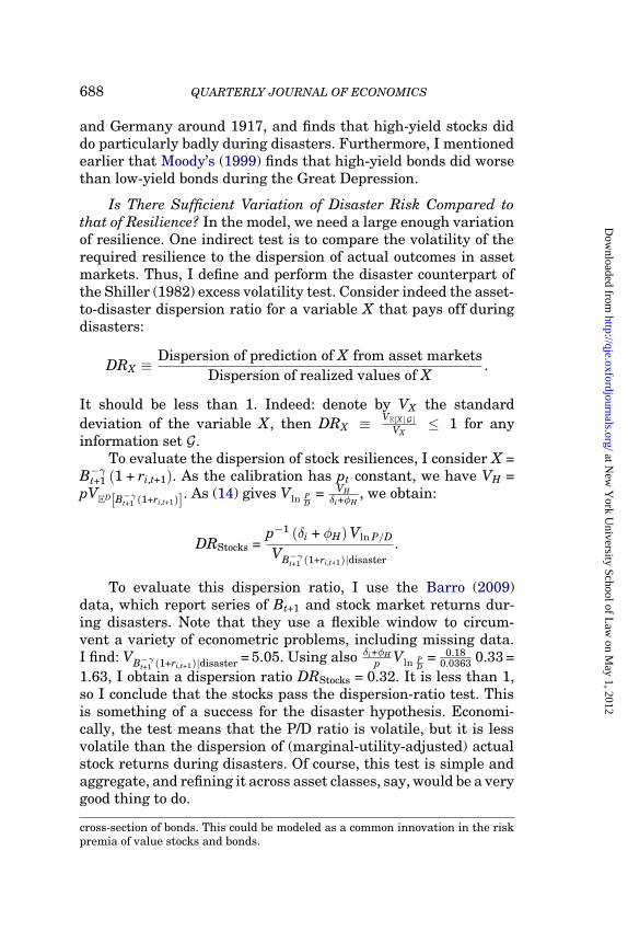
688 QUARTERLY JOURNAL OF ECONOMICS
and Germany around 1917, and finds that high-yield stocks diddoparticularly badly during disasters. Furthermore, I mentionedearlier that Moody’s (1999) finds that high-yield bonds did worsethan low-yield bonds during the Great Depression.
Is There Sufficient Variation of Disaster Risk Compared tothat of Resilience? In the model, we need a large enough variationof resilience. One indirect test is to compare the volatility of therequired resilience to the dispersion of actual outcomes in assetmarkets. Thus, I define and perform the disaster counterpart ofthe Shiller (1982) excess volatility test. Consider indeedthe asset-to-disaster dispersion ratio for a variable X that pays off duringdisasters:
DRX ≡Dispersion of prediction of X from asset markets
Dispersion of realized values of X.
It should be less than 1. Indeed: denote by VX the standarddeviation of the variable X, then DRX ≡
VE[X|G]VX
≤ 1 for anyinformation set G.
To evaluate the dispersion of stock resiliences, I consider X =B−γt+1 (1 + ri,t+1). As the calibration has pt constant, we have VH =pVED[B−γt+1 (1+ri,t+1)]. As (14) gives Vln P
D= VHδi+φH
, we obtain:
DRStocks =p−1 (δi + φH)VlnP/D
VB−γt+1 (1+ri,t+1)|disaster
.
To evaluate this dispersion ratio, I use the Barro (2009)data, which report series of Bt+1 and stock market returns dur-ing disasters. Note that they use a flexible window to circum-vent a variety of econometric problems, including missing data.I find: VB−γt+1 (1+ri,t+1)|disaster = 5.05. Using also δi+φH
p Vln PD
= 0.180.0363 0.33=
1.63, I obtain a dispersion ratio DRStocks = 0.32. It is less than 1,so I conclude that the stocks pass the dispersion-ratio test. Thisis something of a success for the disaster hypothesis. Economi-cally, the test means that the P/D ratio is volatile, but it is lessvolatile than the dispersion of (marginal-utility-adjusted) actualstock returns during disasters. Of course, this test is simple andaggregate, andrefiningit across asset classes, say, wouldbeaverygood thing to do.
cross-section of bonds. This could be modeled as a common innovation in the riskpremia of value stocks and bonds.
at New
York U
niversity School of Law
on May 1, 2012
http://qje.oxfordjournals.org/D
ownloaded from

VARIABLE RARE DISASTERS 689
For inflation, I use the similar reason for the change ininflation during a disaster, X = ΔIt. As Vπ = pVB−γt+1 ΔIt+1
, the dis-
persion ratio is: DRInflation = VπpV
B−γt+1 (ΔIt+1)|disaster
. The calibration gives
Vπ = 2.1%, and the empirical value is VB−γt+1 (ΔIt+1)|disaster = 6.36,so that DRInflation = 0.09. The dispersion ratio is less than 1,consistent with the disaster hypothesis. I conclude that the raredisaster model passes the dispersion-ratio test, for both stocksandinflation. There is enough dispersion in the realizedoutcomesduring disasters towarrant the volatility of stock and bond pricesin samples without disasters.
Do Variations in Recovery Rates Implied by the Model MakeSense? For stocks, the P/D ratio reflects resilience in the model.For instance, the lowP/D ratioin the 1930s and1970s reflects thefact that agents believed that if there was going to be a disaster,the stock market would do terribly. This seems reasonable, giventhe recent experience. Likewise, the measured subjective riskpremia for bonds rise and peak between 1975 and 1982 (Piazzesiand Schneider 2011). In terms of the model, agents reasoned:“if there is a disaster, inflation will really go up.” This seemssensible given their experience with a (nondisaster) crisis andthe concomitant rise in inflation. It would be insightful to have away of formalizing that intuition and probing it, for example, viaa learning model. More broadly, a learning model of how agentsmight form beliefs about disasters, andconditional asset behaviorin disasters, would seem to be quite useful and an important newfrontier for research on time-varying assessment of disaster risk.
VI. CONCLUSION
This articlepresents a tractablewaytohandlea time-varyingseverity of rare disasters, demonstrates its impact on stock andbond prices, and shows its implications for time-varying riskpremia and asset predictability. Many finance puzzles can beunderstood through the lens of the variable rare disasters model.On the other hand, the model does suffer from several limitationsand suggests several questions for future research.
First, it would be useful to empirically examine the model’sjoint expression of the values of stocks, bonds, and options. HereI have only examined their behavior separately, relying on ro-bust stylized facts from many decades of research. The presentstudy suggests specifications for joint cross-asset patterns of
at New
York U
niversity School of Law
on May 1, 2012
http://qje.oxfordjournals.org/D
ownloaded from

690 QUARTERLY JOURNAL OF ECONOMICS
predictability. Themultifactorextensionofthemodel presentedinthe Online Appendix could be instrumental in such an endeavor.
It would be useful to understand how investors estimatedisaster risk. Risk premia seem to decrease following good newsfor the economy (Campbell and Cochrane 1999) and for individ-ual firms (the growth-firms effect). So it seems that updatingwill involve resiliences increasing following good news about thefundamental values of the economy or about individual stocks.Modeling this idea would lead to a link between recent events,risk premia, and future predictability.
This model brings us one step closer to a unified frameworkfor various puzzles in macroeconomics and finance. A companionpaper (Farhi and Gabaix 2011) suggests that various puzzles ininternational macroeconomics (including the forward premiumpuzzle and the excess volatility puzzle on exchange rates) canbe accounted for in an international version of the variable raredisasters framework. Furthermore, ongoing work (Gabaix 2011;Gourio2011) shows howtoembedthe rare-disasters idea in a pro-duction economy by modifying its asset pricing properties whilepreserving its business-cycle properties, producing realistic em-pirical results. Thus, variable rare disaster modeling may bringus closer to the long-sought goal of a joint, tractable frameworkfor macroeconomics and finance.
APPENDIX
Notations
The article often uses a decomposition of a generic variableXt as follows: Xt = X∗ + Xt, where X∗ is a constant part (or“typical value”) and Xt a variable part centered around 0. εX
t+1 isan innovation toX, andσX , its standarddeviation, is the volatilityof variable Xt. The other notations are as follows.
Bt+1 : recovery rate of consumption in a disaster
B = E[B−γt+1
]− 1γ : risk-adjusted average Bt+1
βT : slope in a predictive regression with horizon Tχ : in Epstein-Zin, χ = 1−1/ψ
1−γ , which is 1 in thepower utility case
Dit : dividend of stock iδ : “Ramsey” discount rateδi : stock i’s effective discount rate
at New
York U
niversity School of Law
on May 1, 2012
http://qje.oxfordjournals.org/D
ownloaded from

VARIABLE RARE DISASTERS 691
EDt [Xt+1] (resp. END
t [Xt+1]): expected value conditional on adisaster (resp. on no disaster)
ft (T) : nominal forward rate of maturity TF$t : recovery rate of a nominal dollarFit : recovery rate of stock igC : growth rate of consumptiongiD : growth rate of stock i’s dividendγ : coefficient of relative risk aversionHit : resilience of stock iHEZ
it : Epstein-Zin-enriched resilience of stock iH$ : resilience of a nominal dollarIt : inflationI∗∗ : risk-adjusted central part of inflationJt : jump in inflation in a disasterκ : inflation disaster risk premiumKT : loading on bond risk premiumMt : pricing kernelμit : expected growth of the stock price, conditional on no
disasters (only used for options)pt : disaster probabilityPit : price of stock iπt : variable part of the bond risk premiumφX : rate of mean reversion of variable Xt
ψ : intertemporal elasticity of substitutionψX : rate of mean reversion of variable Xt under the
risk-adjusted measurerf : risk-free ratere
it : stock i’s expected stock return, over a one-period horizonrit→t+T : stock i’s expected stock return, over a horizon Tre$t (T) : expected return on a nominal bond of maturity Tρ : subjective rate of time preferencet : calendar timeT : maturity (for a bond) or horizon (for a regression)VX : dispersion (standard deviation of the distribution) of
variable Xyi : yield on the debt of corporation iyt (T) : nominal yield of maturity TZ$t (T) : price of a nominal zero-coupon bond of maturity T
Exact Setup and Results for the Epstein-Zin Model. Here arethe exact postulates for the EZ model, which lead to closed forms.
at New
York U
niversity School of Law
on May 1, 2012
http://qje.oxfordjournals.org/D
ownloaded from

692 QUARTERLY JOURNAL OF ECONOMICS
I postulate that the variable part of resilience can be writtenas Hct = kt + 1−χ
2 w2 (kt), with a process kt following
(35)dkt=− (φc + χkt) ktdt+(δc + φc + χkt) [(χ− 1)w2 (kt)dt + w (kt)dzt] ,
where zt is a standard Brownian motion.32 Up to second-orderterms, the interpretation is Hct ' kt and dkt ' −φcktdt+ noise,that is, Hct mean-reverts with speed φc. For tractability, theprocess is best expressed with the primitive kt rather than Hct.The volatility function w can be arbitrary, except that it vanishesbefore kt hits −φc
χ(as in Gabaix 2009). This postulate has two
joint consequences, derived in the Online Appendix. The price ofa consumption claim obtains in exact closed form:
(36) Pt =Ct
δc
(
1 +χkt
δc + φc
)
.
In addition, the SDF Mt follows:
dMt
Mt−=−δdt + (χ− 1)
((
Hct +χw2 (kt)
2
)
dt−w (kt)dzt
)
+(B−γt − 1
)dJt,(37)
where dJt is the disaster jump process, equal to 1 with prob-ability ptdt, and otherwise equal to 0. As a result, rft = δ −
(χ− 1)(
Hct + χw2(kt)2
)− ptED
t
[B−γt − 1
]. The interpretation for
both is that in the main text, where the second-order term χw2(kt)2
is neglected.The Epstein-Zin enriched resilience of a stock i is defined as:
(38) HEZit = Hit + (χ− 1)
(
Hct +χw2 (kt)
2
)
+
⟨dMt
Mt,
dDit
Dit
⟩ND
,
where Hit = ptEDt
[B−γt Fit − 1
]and〈dxt, dyt〉
ND dt : = covND(dxt, dyt)is the normal-times (i.e., conditional on No Disaster) covariance
32. The reader might ask: why those postulates? I tried tohave PtCt
= 1+xtδc
, withxt a small term meanreverting at speedφc, and allowed toadd second-order termsto its equation of motion. That generates movements in the SDF, which in turngenerate the price of a consumption claim. Toensure self-consistency andfind Pt
Ct=
1+xtδc
whilehaving MtCt (1, xt) anLG process, there is very little freedom. Basically,one is more or less directly led to postulate (35). Hence, in the spirit of Campbell-Cochane (1995), Gabaix (2009), and this article, I (proudly) reverse-engineeredsecond-order terms to make the first-order economics transparent.
at New
York U
niversity School of Law
on May 1, 2012
http://qje.oxfordjournals.org/D
ownloaded from

VARIABLE RARE DISASTERS 693
between two processes xt and yt. Hence HEZit ' Hit + (χ− 1)Hct,
that is, the EZ resilience is the power utility asset-specific re-silience (Hit) plus an asset-independent term that reflects vari-ations in the interest rate ((χ− 1)Hct). I posit that it follows anLG-twisted process: HEZ
it = HEZi∗ + HEZ
it , with
dHEZit +
⟨dMt
Mt+
dDit
Dit, dNEZ
it
⟩ND
dt(39)
=−(φH + HEZ
it
)HEZ
it dt + dNEZit ,
wheredNEZit is amean-zeroinnovationtoHEZ
it . Thesmall LGtermsarelargelymathematical conveniences that ensurethat themodelis solvedinclosedform, but theinterpretationof the leadingorderis easy: dHEZ
it ' −φHHEZit dt+noise, that is, HEZ
it mean-reverts witha speed φH.
Then, the Online Appendix proves Proposition 9. It is easy tocheckthat thestockpriceis higherif thedividends covarywiththeprice kernel in normal times, or if resilience innovations covarywith it. One can easily verify that HEZ
ct =χkt, which elucidates themeaning of kt: up to a multiplicative factor, it is the variable partof the EZ-enriched resilience of a consumption claim.
Proof of Theorem 1. Following the general procedure for LGprocesses, I use (2), (3), and form:
Mt+1Di,t+1
MtDit= e−δ+giD
(1 + εD
t+1
)
×
{1 if there is no disaster at t + 1B−γt+1Fi,t+1 if there is a disaster at t + 1
.
As the probability of disasters at t + 1 is pt, and Hit ≡pt(Et[B−γt+1Fi,t+1
]− 1),
Et
[Mt+1Di,t+1
MtDit
]
= e−δ+giD{ (1− pt) ∙ 1︸ ︷︷ ︸No disaster term
+ pt ∙ Et[B−γt+1Fi,t+1
]
︸ ︷︷ ︸Disaster term
}
= e−δ+giD (1 + Hit) = e−δ+giD
(1 + Hi∗ + Hit
)
(40)= e−δ+giD+hi∗
(1 + e−hi∗Hit
)
= e−δi
(1 + e−hi∗Hit
),
at New
York U
niversity School of Law
on May 1, 2012
http://qje.oxfordjournals.org/D
ownloaded from

694 QUARTERLY JOURNAL OF ECONOMICS
where I use the notations hi∗ = ln (1 + Hi∗) and δi = δ − giD − hi∗.Next, as Hi,t+1 is independent of whether there is a disaster, andis uncorrelated with εD
t+1,
Et
[Mt+1Di,t+1
MtDitHi,t+1
]
= Et
[Mt+1Di,t+1
MtDit
]
Et
[Hi,t+1
]
= e−δ+giD (1 + Hit) ∙1 + Hi∗
1 + Hite−φH Hit(41)
= e−δ+giD+hi∗−φH Hit = e−δi−φH Hit.
Weseethat in(5) thereasonforthe1+Hit terminthedenominatorwas to ensure that the above expression would remain linearin Hit.
There are two ways to conclude. The first way (which is notentirely rigorous, but is elementary) is to look for a solution of thetype Pit =Dit
(a + bHit
)for some constants a andb. The price must
satisfy: Pit = Dit + E[
Mt+1Pi,t+1Mt
], that is, for all Hit,
a + bHit = 1 + Et
[Mt+1Di,t+1
MtDit
(a + bHi,t+1
)]
= 1 + aEt
[Mt+1Di,t+1
MtDit
]
+ bEt
[Mt+1Di,t+1
MtDitHi,t+1
]
= 1 + ae−δi
(1 + e−hi∗Hit
)+ be−δi−φHit =
(1 + ae−δi
)
+(
ae−δi−hi∗ + be−δi−φH
)Hit.
Solving for a and b, we get a = 1 + ae−δi , b = ae−δi−hi∗ + be−δi−φH ,and (13).
The second way is rigorous, and uses linearity-generating(LG) processes. A very short summary of the machinery is avail-able on my web page, and the reader is encouraged to referto it for the following argument and the proof of Theorem 2.Equations (40)and(41)ensurethat MtDit
(1, Hit
)is anLGprocess
with generator
(e−δi e−δi−hi∗
0 e−δi−φH
)
. The stock price (13) comes from
Theorem 2 in Gabaix (2009).
Proof of Theorem 2. The proof is simpler when J∗ = κ = 0, andthis is the best case to keep in mind in a first reading. I call ρI =e−φI and ρJ = e−φJ , use the inflation-adjusted (i.e., real) face value
at New
York U
niversity School of Law
on May 1, 2012
http://qje.oxfordjournals.org/D
ownloaded from

VARIABLE RARE DISASTERS 695
of the bond, Qt, so that Qt+1Qt
= (1− It) in normal times, and Qt+1Qt
=(1− It)F$,t+1 if there is a disaster. I calculate the LG moments.
Et
[Mt+1Qt+1
MtQt
]
= e−δ (1− It) {(1− pt) ∙ 1 + pt ∙ Et[B−γt+1F$,t+1
]}
= e−δ (1 + H$)(
1− I∗ − It
).
Et
[Mt+1Qt+1
MtQtIt+1
]
= e−δ (1− It) {(1− pt)ENDt
[It+1
]+ pt ∙ E
Dt
[B−γt+1F$,t+1It+1
]}
= e−δ (1− It)1− I∗1− It
{(1− pt + ptEt
[B−γt+1F$,t+1
])× ρIIt
+ ptEt[B−γt+1F$,t+1
] (J∗ + Jt
)}
= e−δ (1 + H$) (1− I∗)
(
ρIIt +ptEt
[B−γt+1F$,t+1
]
1 + H$
(J∗ + Jt
))
= Ψ(ρIIt + (1− I∗)κ (1− ρI − κ) + πt
),
Ψ ≡ e−δ (1 + H$) (1− I∗)
using (8) and (9). This gives:
Et
[Mt+1Qt+1
MtQt
It+1
1− I∗
]
= Ψ
(
κ (1− ρI − κ) + ρIIt
1− I∗+
πt
1− I∗
)
Et
[Mt+1Qt+1
MtQtJt+1
]
= Et
[Mt+1Qt+1
MtQt
]
Et
[Jt+1
]= Ψ
1− I∗1− It
ρJJt+1
= ΨρJJt+1,
so that, as πt1−I∗
is proportional to Jt (equation (8)),
Et
[Mt+1Qt+1
MtQt
πt+11−I∗
]= ΨρJ
πt+11−I∗
. Hence, MtQt
(1, It
1−I∗, πt
1−I∗
)is an LG
process with generator Ω = Ψ
1 −1 0
κ (1− ρI − κ) ρI 10 0 ρπ
. Theorem 1
in Gabaix (2009) gives the bond price, Z$t (T) = (1, 0, 0)ΩT(
1, It1−I∗
, πt1−I∗
)′, which concludes the derivation of (16) when
κ = 0. When κ /= 0, one more step is required. The eigenvaluesof Ω are Ψ {1− κ, ρI + κ, ρπ}. It is convenient to factorize by1 − κ and, hence, to define: ρi = ρI+κ
1−κ and ρπ = ρπ1−κ , which are the
at New
York U
niversity School of Law
on May 1, 2012
http://qje.oxfordjournals.org/D
ownloaded from

696 QUARTERLY JOURNAL OF ECONOMICS
discrete-time analogues of the continuous-time mean-reversionspeeds ψI ≡ φI − 2κ and ψJ ≡ φJ − κ. Calculating ΩT gives thebond price:
Z$t (T) = (Ψ (1− κ))T ×
{
1−1
1− κ1− ρT
i
1− ρi
(It
1− I∗− κ
)
(42)
−1
(1− κ)2∙
1−ρTi
1−ρi− 1−ρT
π
1−ρπ
ρi − ρπ∙
πt
1− I∗
.
The corresponding value of the yield yt (T) =− lnZ$t(T)T is:
yt (T) = δ −H$ + I∗∗ +1− e−ψIT
ψIT(It − I∗∗)
(43)
+1−e−ψIT
ψI− 1−e−ψJ T
ψI
(ψJ − ψI)Tπt + O (It − I∗∗,πt)
2
= δ −H$ + It + (κ (φI − κ) + πt − φI (It − I∗))T2
.(44)
Proof of Proposition 3. We have Vt = VNDt + VD
t with:
VNDt = (1− pt)E
NDt [e
−δ
(
K −Pi,t+1
Pit
)+
] = (1− pt) e−δ
× Et
[(K − eμ+σut+1−σ
2/2)+]
VDt = ptE
Dt
[
e−δ(
B−γt+1K −Pi,t+1
Pit
)+]
= pte−δEt
[B−γt+1 (K − eμFi,t+1)
+] ,
where x+ =max (0, x). Recall that the Black-Scholes value of a putwithmaturity1 is: Et[e−r(K−er+σut+1−σ
2/2)+]=VBSPut (Ke−r,σ). Hence,
the first term is (1− pt) times:
e−δEt[(K − eμ+σut+1−σ2/2)+] = e−δ+μEt[(Ke−μ − eμ+σut+1−σ
2/2)+]
= e−δ+μVBSPut
(Ke−μ,σ
).
Proof of Proposition 6. The Fama-Bliss regression (28) yields
βT =cov(re
$t(T)−re$t(0),ft(T)−ft(0))
var(ft(T)−ft(0)). Equations (17) and (21) give re
$t (T)−
re$t (0) = 1−e−ψIT
ψIπt + O
(It,πt
)2and
at New
York U
niversity School of Law
on May 1, 2012
http://qje.oxfordjournals.org/D
ownloaded from

VARIABLE RARE DISASTERS 697
ft (T)− ft (0) =(e−ψIT − 1
)It +
e−ψIT − e−ψJT
ψJ − ψIπt + aT + O
(It,πt
)2,
where aT is a constant. So to the leading order,
(45) βT =e−ψIT−e−ψJ T
ψJ−ψI∙ 1−e−ψIT
ψIvar (πt)
var((e−ψIT − 1) It + e−ψIT−e−ψJ T
ψJ−ψIπt
) ,
which implies that limT→∞ βT = 0, limT→0 βT = var(πt)var(ψI It+πt)
, and (29).
Proof of Proposition 7. This proof is in the limit of σI → 0,It = 0, κ → 0, andΔt → 0. Equation 43 gives: yt (T) = a + b (T)πt,
with b (T) =1−e−ψIT
ψI− 1−e−ψJ T
ψI(ψJ−ψI)T
= T2 −
ψI+ψJ6 T2 + O (T3). Hence:
yt+Δt (T −Δt)− yt (T)Δt
=Et [dyt (T)]
dt−∂yt (T)∂T
= (−φJb (T)− b′ (T))πt.
As yt(T)−rt
T = b(T)πt
T , −β = φJb(T)+b′(T)b(T)/T , that is,
(46) β =−Tb′ (T)b (T)
− φJT,
sothat β =−1− 2ψj−ψI
3 T +O (T2)when T → 0, andβ =−ψJT +o (T)when T →∞. The reasoning in the text of the article comes fromthefact that forsmall T, Et[dyt(T)]
dt =−φJT2 πt,−
∂yt(T)∂T =
(− 1
2 + O (T))πt,
so yt+Δt(T−Δt)−yt(T)Δt ' −∂yt(T)
∂T .
NEW YORK UNIVERSITY
SUPPLEMENTARY MATERIAL
An Online Appendix for this article can be found at QJEonline (qje.oxfordjournals.org).
REFERENCES
Almeida, Heitor, and Thomas Philippon, “The Risk-Adjusted Cost of FinancialDistress,” Journal of Finance, 62 (2007), 2557–2586.
Amihud, Yakov, and Avi Wohl, “Political News and Stock Prices: The Case ofSaddam Hussein Contracts,” Journal of Banking and Finance, 28 (2004),1185–1200.
at New
York U
niversity School of Law
on May 1, 2012
http://qje.oxfordjournals.org/D
ownloaded from

698 QUARTERLY JOURNAL OF ECONOMICS
Backus, David, Mikhail Chernov, and Ian Martin, “Disasters Implied by EquityIndex Options,” Journal of Finance (forthcoming).
Bansal, Ravi, and Ivan Shaliastovich, “A Long-Run Risks Explanation of Pre-dictability Puzzles in Bond and Currency Markets,” Working Paper, DukeUniversity, 2009.
Bansal, Ravi, and Amir Yaron, “Risks for the Long Run: A Potential Resolution ofAsset Pricing Puzzles,” Journal of Finance, 59 (2004), 1481–1509.
Barro, Robert, “Rare Disasters and Asset Markets in the Twentieth Century,”Quarterly Journal of Economics, 121 (2006), 823–866.
———, “Rare Disasters, Asset Prices, and Welfare Costs,” American EconomicReview, 99 (2009), 243–264.
Barro, Robert, and Jose Ursua, “Macroeconomic Crises Since 1870,” BrookingsPapers on Economic Activity (2008), 255–335.
———, “StockMarket Crashes andDepressions,”NBERWorkingPaperno. 14760,2009.
Berkman, Henk, Ben Jacobsen, and John Lee, “Time-Varying Rare Disaster Riskand Stock Returns,” Journal of Financial Economics, 101 (2011), 313–332.
Binsbergen, Jules van, Michael Brandt, and Ralph Koijen, “On the Timing andPricing of Dividends,” American Economic Review (forthcoming).
Bittlingmayer, George, “Output, Stock Volatility, and Political Uncertainy in aNatural Experiment: Germany 1880–1940,” Journal of Finance, 53 (1998),2243–2256.
Bollerslev, Tim, George Tauchen, and Hao Zhou, “Expected Stock Returns andVariance Risk Premia,” Review of Financial Studies, 22 (2009), 4463–4492.
Bollerslev, Tim, and Viktor Todorov, “Tails, Fears and Risk Premia,” Journal ofFinance (forthcoming).
Brandt, Michael W., and Kevin Q. Wang, “Time-Varying Risk Aversion andUnexpectedInflation,” Journal of Monetary Economics, 50 (2003), 1457–1498.
Brown, Stephen, William Goetzmann, and Stephen Ross, “Survival,” Journal ofFinance, 53 (1995), 853–873.
Brunnermeier, Markus, Stefan Nagel, and Lasse Pedersen. “Carry Trades andCurrency Crashes,” NBER Macroeconomics Annual, 23 (2008), 313–347.
Burnside, Craig, Martin Eichenbaum, Isaac Kleshchelski, and Sergio Rebelo, “DoPeso Problems Explain the Returns to the Carry Trade? Review of FinancialStudies 24 (2011), 853–891.
Campbell, John Y., “Consumption-Based Asset Pricing,” in Handbook of theEconomics of Finance, George M. Constantinides, Milton Harris, and ReneM. Stulz, eds. (Amsterdam: Elsevier, North Holland, 2003).
Campbell, John Y., and John Cochrane, “By Force of Habit: A Consumption-Based Explanation of Aggregate Stock Market Behavior,” Journal of PoliticalEconomy, 107 (1999), 205–251.
Campbell, John Y., Andrew W. Lo, and A. Craig MacKinlay, The Econometrics ofFinancial Markets, (Princeton, NJ: Princeton University Press, 1997).
Campbell, John Y., and Robert J. Shiller, “The Dividend-Price Ratio and Expecta-tions of FutureDividends andDiscount Factors,” Review of Financial Studies,1 (1988), 195–228.
———, “Yield Spreads and Interest Rate Movements: A Bird’s Eye View,” Reviewof Economic Studies, 58 (1991), 495–514.
Catao, Luis, and Marco Terrones, “Fiscal Deficits and Inflation,” Journal ofMonetary Economics, 52 (2005), 529–554.
Chen, Hui, Scott Joslin, and Ngoc-Khanh Tran, “Rare Disasters and Risk Sharingwith Heterogeneous Beliefs,” Working Paper, MIT, 2011.
Chen, Long, Pierre Collin-Dufresne, and Robert S. Goldstein, “On the Relationbetween the Credit Spread Puzzle and the Equity Premium Puzzle,” Reviewof Financial Studies, 22 (2009), 3367–3409.
Cochrane, John, “The Dog That DidNot Bark: A Defense of Return Predictability,”Review of Financial Studies, 21 (2008), 1533–1575.
Cochrane, John, and Monika Piazzesi, “Bond Risk Premia,” American EconomicReview, 95 (2005), 138–160.
Cremers, Martijn, Joost Driessen, and Pascal Maenhout, “Explaining the Level ofCredit Spreads: Option-Implied Jump Risk Premia in a Firm Value Model,”Review of Financial Studies, 21 (2008), 2209–2242.
at New
York U
niversity School of Law
on May 1, 2012
http://qje.oxfordjournals.org/D
ownloaded from

VARIABLE RARE DISASTERS 699
Dai, Qiang, and Kenneth J. Singleton, “Expectation Puzzles, Time-Varying RiskPremia, and Affine Models of the Term Structure,”Journal of FinancialEconomics, 63 (2002), 415–441.
Daniel, Kent, and Sheridan Titman, “Evidence on the Characteristics of CrossSectional Variation in Stock Returns,” Journal of Finance, 52 (1997),1–33.
Drechsler, Itamar, and Amir Yaron, “What’s Vol Got to Do with It,” Review ofFinancial Studies, 24 (2011), 1–45.
Du, Du, “General Equilibrium Pricing of Options with Habit Formation andEventRisks,” Journal of Financial Economics, 99 (2011), 400–426.
Duffee, Gregory, “Term Premia and Interest Rate Forecasts in Affine Models,”Journal of Finance, 57 (2002), 405–443.
Dybvig, Philipp, John Ingersoll, andStephen Ross, “Long forwardandzerocouponrates can never fall,” Journal of Business 69 (1996), 1–25.
Epstein, Larry G., and Stanley E. Zin, “Substitution, Risk Aversion, and theTemporal Behavior of Consumption and Asset Returns: A Theoretical Frame-work,” Econometrica, 57 (1989), 937–969.
Fama, EugeneF., andRobert R. Bliss, “TheInformationinLong-MaturityForwardRates,” American Economic Review, 77 (1987), 680–692.
Fama, Eugene F, and Kenneth R. French, “Common Risk Factors in the Re-turns on Stocks and Bonds,” Journal of Financial Economics, 33 (1993),3–56.
Farhi, Emmanuel, and Xavier Gabaix, “Rare Disasters and Exchange Rates,”Working Paper, Harvard University, 2011.
Farhi, Emmanuel, Samuel Fraiberger, Xavier Gabaix, Romain Ranciere, andAdrien Verdelhan, “Crash Risk in Currency Markets,” NBER Working Paperno. 15062, 2009.
Figlewski, Stephen, “Estimating the Implied Risk Neutral Density for the U.S.Market Portfolio,” in Volatility and Time Series Econometrics: Essays inHonor of Robert F. Engle, Tim Bollerslev, Jeffrey Russell, and Mark Watson,eds. (Oxford: Oxford University Press, 2008).
Gabaix, Xavier, “Variable Rare Disasters: A Tractable Theory of Ten Puzzlesin Macro-Finance,” American Economic Review, Papers and Proceedings, 98(2008), 64–67.
———, “Linearity-Generating Processes: A Modelling Tool Yielding Closed Formsfor Asset Prices,” Working Paper, New York Uuniversity, 2009.
———, “Disasterization: A Simple Way to Fix the Asset Pricing Properties ofMacro-economic Models,” American Economic Review, Papers and Proceed-ings, 101 (2011), 406–409.
Gabaix, Xavier, Parameswaran Gopikrishnan, Vasiliki Plerou, and H. EugeneStanley, “A Theory of Power Law Distributions in Financial Market Fluctua-tions,” Nature, 423 (2003), 267–230.
———, “Institutional Investors and Stock Market Volatility,” Quarterly Journalof Economics, 121 (2006), 461–504.
Ghandi, Pryiank, and Hanno Lustig, “A Fiscal Explanation of the Size Anomaliesin U.S. Bank Stock Returns,” Working Paper, University of California, LosAngeles, 2011.
Ghosh, Anisha, and Christian Julliard, “Can Rare Events Explain the EquityPremium Puzzle?,” Working Paper, Carnegie-Mellon University, 2008.
Gourio, Francois, “Disasters and Recoveries,” American Economic Review, Papersand Proceedings, 98 (2008a), 68–73.
———, “Predictability in the Disaster Model,” Finance Research Letters, 5 (2008b),191–203.
———, “Disaster Risk and Business Cycles,” Working Paper, Boston University,2011.
Jackwerth, Jens Carsten, andMark Rubinstein, “Recovering Probability Distribu-tions from Option Prices,” Journal of Finance, 51 (1996), 1611–1631.
Kelly, Bryan, “Tail Risk and Asset Prices,” Working Paper, University of Chicago,2011.
Koijen, Ralph, HannoLustig, andStijnvanNieuwerburgh, “TheCross-SectionandTime-Series of Stock and Bond Returns,” Working Paper, SSRN, 2010.
at New
York U
niversity School of Law
on May 1, 2012
http://qje.oxfordjournals.org/D
ownloaded from

700 QUARTERLY JOURNAL OF ECONOMICS
Kozak, Serhiy, “Bond and Foreign Exchange Risk Premia,” Working Paper, Uni-versity of Chicago, 2011.
Krishnamurthy, Arvind, and Annette Vissing-Jorgensen, “The Demand for Trea-sury Debt,” Working Paper, Northwestern University, 2008.
Lettau, Martin, andStijn van Nieuwerburgh, “Reconciling the Return Predictabil-ity Evidence,” Review of Financial Studies, 21 (2008), 1607–1652.
Lettau, Martin, andJessica Wachter, “The Term Structures of Equity andInterestRates,” Journal of Financial Economics, 101 (2011), 90–113.
Liu, Jun, Jun Pan, and Tan Wang, “An Equilibrium Model of Rare Event Premia,”Review of Financial Studies, 18 (2005), 131–164.
Longstaff, Francis, and Monika Piazzesi, “Corporate Earnings and the EquityPremium,” Journal of Financial Economics, 74 (2004), 401–421.
Macaulay, Frederick, Some Theoretical Problems Suggested by the Movement ofInterest Rates, Bond Yields and Stock Prices in the United States since 1856(New York: NBER, 1938).
Mehra, Rajnish, and Edward Prescott, “The Equity Premium: A Puzzle,” Journalof Monetary Economics, 15 (1985), 145–161.
Moody’s, “Historical Default Rates of Corporate Bond Issuers, 1920–1996,” inHigh Yield Bonds: Market Structure, Portfolio Management, and Credit Risk,TheodoreM. Barnhill, WilliamF. Maxwell, andMarkR. Shenkman, eds. (NewYork: McGraw-Hill, 1999).
Nakamura, Emi, Jon Steinsson, Robert Barro, and Jose Ursua, “Crises andRecoveries in an Empirical Model of Consumption Disasters,”Working Paper,Harvard University, 2011.
Piazzesi, Monika, and Martin Schneider, “Equilibrium Yield Curves,” NBERMacroeconomics Annual, 21 (2007), 389–442.
———, “Trend and Cycle in Bond Premia,” Working Paper, Stanford University,2011.
Rietz, Thomas, “The Equity Risk Premium: A Solution,” Journal of MonetaryEconomics, 22 (1988), 117–131.
Santa-Clara, Pedro, and Shu Yan, “Crashes, Volatility, and the Equity Premium:Lessons from S&P 500 Options,” Review of Economics and Statistics, 92(2010), 435–451.
Shiller, Robert, “Do Stock Prices Move Too Much to Be Justified by SubsequentChanges in Dividends?,” American Economic Review, 71 (1981), 421–436.
Veronesi, Pietro, “The Peso Problem Hypothesis and Stock Market Returns,”Journal of Economic Dynamics and Control, 28 (2004), 707–725.
Viceira, Luis, “Bond Risk, Bond Return Volatility, and the Term Structure ofInterest Rates”, Working paper 07–082, Harvard Business School, 2007.
Wachter, Jessica, “A Consumption-Based Model of the Term Structure of InterestRates,” Journal of Financial Economics, 79 (2006), 365–399.
Wachter, Jessica, “Can Time-Varying Risk of Rare Disasters Explain AggregateStock Market Volatility?,” NBER Working Paper no. 14386, 2009.
Weil, Philippe, “The Equity Premium Puzzle and the Risk-Free Rate Puzzle,”Journal of Monetary Economics, 24 (1990), 401–421.
Weitzman, Martin, “SubjectiveExpectations andAsset-ReturnPuzzles,”AmericanEconomic Review, 97 (2007), 1102–1130.
at New
York U
niversity School of Law
on May 1, 2012
http://qje.oxfordjournals.org/D
ownloaded from