Chapter 7 DIMENSIONAL ANALYSIS AND SIMILITUDE ◎ Because so few real flows can be solved exactly by analytical

methods alone, the development of fluid mechanics has depended heavily on experimental results.

◎ Experimental work in the laboratory is both time-consuming and expensive. One obvious goal is to obtain the most information from the fewest experiments.

◎ Dimensional analysis is an important tool that often helps us to achieve this goal.

◎ The dimensionless parameters that we obtain also can be used to correlate data for presentation using the minimum possible number of plots.

◎ When experimental testing of a full-size prototype is either impossible or prohibitively expensive, the only feasible way of

attacking the problem is through model testing in the laboratory. ◎ If we are to predict the prototype behavior from measurements

on the model, it is obvious that we cannot run just any test on any model. The model flow and the prototype flow must be related by known scaling laws.

7.1 Nature of Dimensional Analysis ◎ Most phenomena in fluid mechanics depend in a complex way

on geometric and flow parameters. ◎ Determine the drag force on a sphere: F=f(D, V, ρ, μ)? ◎ If the experimental procedure were repeated for 10 values of

each variable, simple arithmetic shows that 104 separated tests would be needed.

◎ Assuming each test takes 0.5 hour and we work 8 hours per

day, the testing will require 2.5 years to complete. Needless to say, there also would be some difficulty in presenting the data.

◎ Fortunately, we can obtain meaningful results with significantly less effort through the use of dimensional analysis.

12 2

F VDfV D

ρρ μ

⎛ ⎞= ⎜ ⎟

⎝ ⎠

◎ The form of the function still must be determined experimentally. However, rather than needing to conduct 104 experiments, we could establish the nature of the function as accurately with only 10 tests.

◎ The Buckingham Pi theorem is a statement of the relation between a function expressed in terms of dimensional parameters and a related function expressed in terms of nondimensional

parameters. ◎ Use of the Buckingham Pi theorem allows us to develop the

important nondimensional parameters quickly and easily. 7.2 Buckingham Pi Theorem ◎ Given a physical problem in which the dependent parameter is

a function of n-1 independent parameters, we may express the relationship among the variables in functional form as

q1=f(q2, q3,…..qn) where q1 is the dependent parameter, and q2, q3, …, qn are the n-1 independent parameters. ◎ Mathematically, we can express the functional relationship in

the equivalent form g(q1, q2, q3,…..qn)=0

where g is an unspecified function, different from f.

7.3 Determing The Π Groups

◎ The functional relationship among the Π parameters must be

determined experimentally.

◎ The procedure outlined above, where m is taken equal to r (the

fewest independent dimensions required to specify the dimensions of all parameters involved) almost always produces the correct number of dimensionless Π parameters.

◎ In a few cases, trouble arises because the number of primary dimensions differs when variables are expressed in terms of different systems of dimensions, the value of m can be established with certainty by determing the rank of the

dimensional matrix; that rank is m. ◎ The n-m dimensionless groups obtained from the procedure

are independent but not unique. ◎ Experience suggests that viscosity should appear in only one

dimensionless parameter. Therefore μ should not be chosen as a repeating parameter.

◎ Choosing density ρ, with dimensions M/L3, velocity V, with dimensions L/T, and characteristic length L, with dimension L, as repeating parameters generally leads to a set dimensionless parameters that are suitable for correlating a wide range of experimental data.

7.4 Significant Dimensionless Groups in Fluid Mechanics ◎ Forces encountered in flowing fluids include those due to

inertial, viscosity, pressure, gravity, surface tension, and compressibility.

◎ The ratio of any two forces will be dimensionless. We have previously shown that the inertial force is proportional to ρV2L2. To facilitate forming ratios of forces, we can express each of the remaining forces as follows:

◎ Inertia forces are important in most fluid mechanics problems.

The ratio of the inertia force to each of the other forces listed above leads to five fundamental dimensionless groups encountered in fluid mechanics.

◎ Reynolds number, Re: the ratio of inertia forces to viscous forces. Flows with “large” Re generally are turbulent. Flows in which the inertia forces are “small” compared with the viscous forces are characteristically laminar flows.

2 2

Re VL V LVL

ρ ρμ μ

= =

◎ Euler number (Pressure Coefficient, CP), Eu: the ratio of pressure forces to inertial forces. The factor 1/2 is introduced into the denominator to give the dynamic pressure. In the study of cavitation phenomena, the pressure difference, Δp, is taken as

Δp=p-pv, where p is the pressure in the liquid stream, and pv is the liquid vapor pressure at the test temperature. Combining with ρ and V in the stream yields the dimensionless parameter called the Cavitation number, Ca.

2

2 2 21 12 2

p pLEuV V Lρ ρ

Δ Δ= = ,

212

vp pCaVρ

−=

◎ Froude number, Fr: the ratio of inertial forces to gravity forces. Fr less that unity indicate subcritical flow and values greater than unity indicate supercritical flow.

2 2 22

3

V V LFrgL g L

ρρ

= =

◎ Weber number, We: the ratio of inertial forces to surface

tension forces. 2 2 2V L V LWe

Lρ ρσ σ

= =

◎ Mach number, Ma: the ratio of inertial forces to forces due to compressibility. For truly incompressible flow (under some conditions even liquids are quite compressible), c= ∞ so that M=0.

2 22

2, vv

V V V V LM Mc E Ldp E

d

ρ

ρ ρ

= = = =

7.5 Flow Similarity and Model Studies ◎ To be useful, a model test must yield data that can be scaled to

obtain the forces, moments, and dynamic loads that would exist on the full-scale prototype. What conditions must be met to ensure the similarity of model and prototype flows?

◎ Geometric similarity: the model and prototype must be the same shape, and that all linear dimensions of the model be related to corresponding dimensions of the prototype by a constant scale factor.

◎ Kinematic similarity: Two flows are kinematically similar when the velocities at corresponding points are in the same direction and are related in magnitude by a constant scale factor. Thus two flows that are kinematically similar also have streamline patterns related by a constant scale factor. Since the boundaries form the bounding streamlines, flows that are kinematically similar must be geometrically similar.

◎ If compressibility or cavitation effects, which may change even the qualitative patterns of flow, are not present in the prototype flow, they must be avoided in the model flow.

◎ Dynamic similarity: when two flows have force distributions such that identical types of forces are parallel and are related in magnitude by a constant scale factor at all corresponding points, the flows are dynamically similar.

◎ The requirements for dynamic similarity are the most restrictive. Kinematic similarity requires geometric similarity; kinematic similarity is a necessary, but not sufficient, requirement for dynamic similarity.

◎ To establish the conditions required for complete dynamic similarity, all forces (viscous forces, pressure forces, surface tension forces, etc.) that are important in the flow situation must

be considered. Test conditions must be established such that all important forces are related by the same scale factor between model and prototype flows. What are the conditions for ensuring dynamic similarity between model and prototype flow?

◎ The Buckingham Pi theorem may be used to obtain the governing dimensionless groups for a flow phenomenon; to achieve dynamic similarity between geometrically similar flows, we must duplicate the independent dimensionless groups; by so doing the dependent parameter is then duplicated.

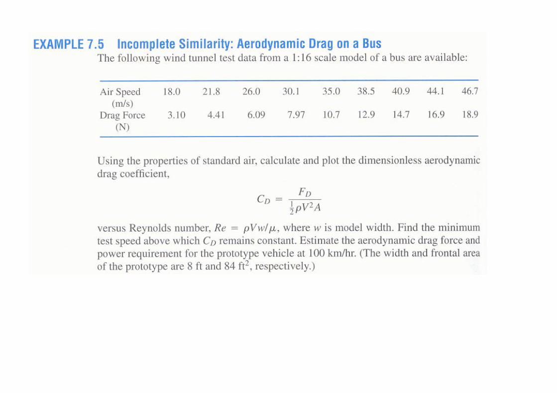
7.5.1 Incomplete Similarity ◎ We have shown that to achieve complete dynamic similarity

between geometrically similar flows, it is necessary to duplicate the independent dimensionless groups; by so doing the dependent parameter is then duplicated.

◎ In many model studies, to achieve dynamic similarity requires duplication of several dimensionless groups. In some cases, complete dynamic similarity between model and prototype may not be attainable.

◎ Determining the drag force of a surface ship is an example of such a situation. Resistance on a surface ship arises from skin friction on the hull (viscous forces) and surface wave resistance (gravity forces). Complete dynamic similarity requires that both Reynolds and Froude numbers be duplicated between model and

prototype. ◎ In general it is not possible to predict wave resistance

analytically, so it must be modeled. This requires that

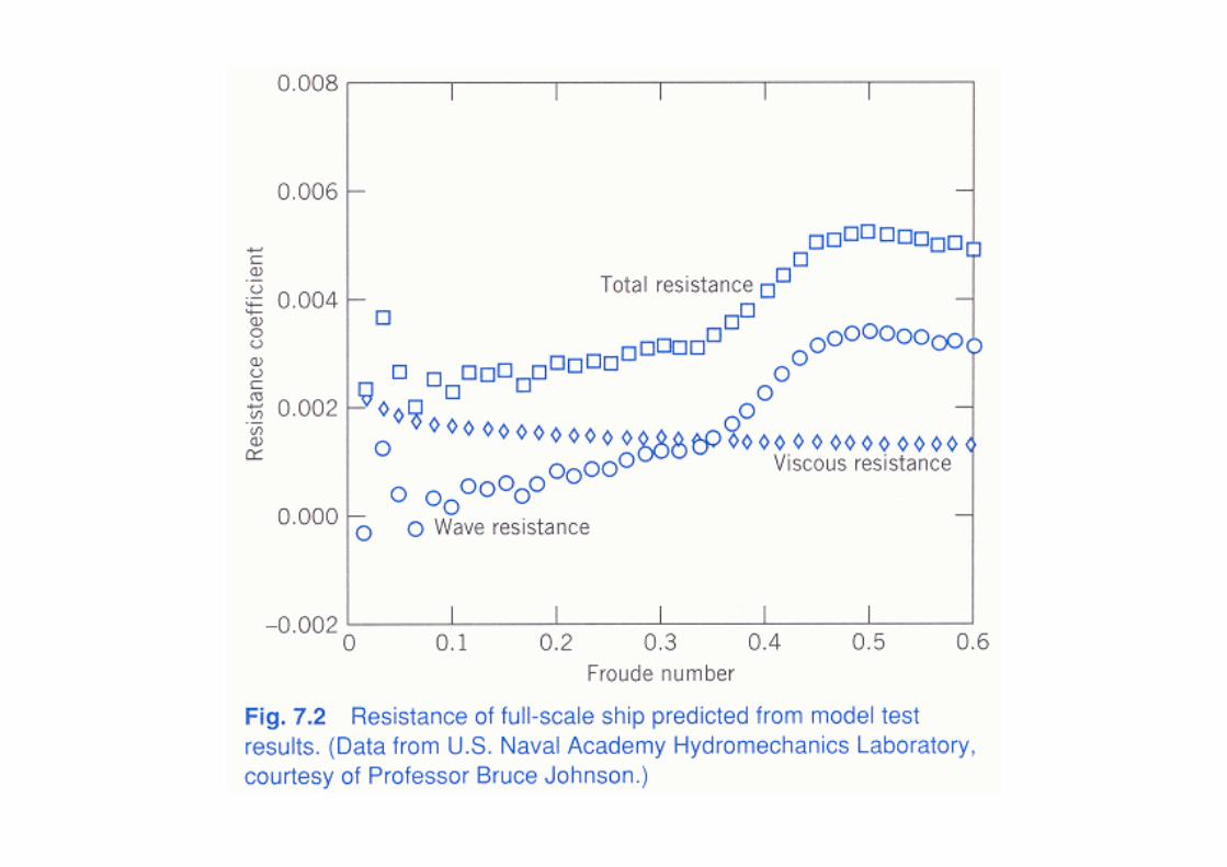
◎ The square points are calculated from values of total resistance measured in the model test.

◎ Resistance of the full-scale ship can be calculated from model test results using the following procedure.

◎ The viscous drag on the model is estimated using the analytical methods. The estimated frictional resistance coefficients are plotted in Fig. 7.1 as diamonds.

◎ The model wave resistance is calculated as the difference between total drag and estimated friction drag. The estimated wave-resistance coefficients for the model are plotted as circles.

◎ The prototype wave resistance is calculated using Froude number scaling by equating wave-resistance coefficients for model and prototype. The points plotted as circles in Fig. 7.2 for the prototype are identical to model coefficients at corresponding

Froude numbers. ◎ The skin friction drag calculated analytically for the prototype,

shown in Fig. 7.2 by the diamonds, is added to the scaled wave-drag coefficients to predict the total drag coefficients for the prototype (square points).

◎ Because the Re cannot be matched for model tests of surface ships, the BL behavior is not the same for model and prototype. The Re is only (Lm/Lp)3/2 as large as the prototype value. The model BL is “tripped” or “stimulated” to become turbulent at a location that corresponds to the behavior on the full-scale vessel. “Studs” were used to stimulate the BL for the model test results shown in Fig. 7.1.

◎ A correction sometimes is added to the full-scale coefficients calculated from model test data. This correction accounts for

roughness, waviness, and unevenness that inevitably are more pronounced on the full-scale ship than on the model.

◎ Comparisons between predictions from model tests and measurements made in full-scale trials suggest an overall accuracy within ±5 percent.

7.6 Nondimensionalizing the Basic Differential Equations