Variability of particulate organic carbon concentration in the north polar

Atlantic based on ocean color observations with Sea-viewing Wide Field-of-

view Sensor (SeaWiFS)

Malgorzata Stramska

Hancock Institute for Marine Studies, University of Southern California, Los Angeles,

California, USA

Dariusz Stramski

Marine Physical Laboratory, Scripps Institution of Oceanography, University of California at

San Diego, La Jolla, California, USA

Complete citation: Stramska, M., and D. Stramski (2005), Variability of particulate organic carbon

concentration in the north polar Atlantic based on ocean color observations with Sea-viewing Wide Field-

of-view Sensor (SeaWiFS), J. Geophys. Res., 110, XXXXXX, doi:10.1029/2004JC002762.

1

https://ntrs.nasa.gov/search.jsp?R=20050223592 2018-08-26T17:14:58+00:00Z

Abstract. We use satellite data from Sea-viewing Wide Field-of-view Sensor (SeaWiFS) to

investigate distributions of particulate organic carbon (POC) concentration in surface waters of

the north polar Atlantic Ocean during the spring–summer season (April through August) over a

6-year period from 1998 through 2003. By use of field data collected at sea, we developed

regional relationships for the purpose of estimating POC from remote-sensing observations of

ocean color. Analysis of several approaches used in the POC algorithm development and match-

up analysis of coincident in situ–derived and satellite-derived estimates of POC resulted in

selection of an algorithm that is based on the blue-to-green ratio of remote-sensing reflectance

Rrs (or normalized water-leaving radiance Lwn). The application of the selected algorithm to a 6-

year record of SeaWiFS monthly composite data of Lwn revealed patterns of seasonal and

interannual variability of POC in the study region. For example, the results show a clear increase

of POC throughout the season. The lowest values, generally less than 200 mg m–3, and at some

locations often less than 50 mg m–3, were observed in April. In May and June, POC can exceed

300 or even 400 mg m–3 in some parts of the study region. Patterns of interannual variability are

intricate, as they depend on the geographic location within the study region and particular time of

year (month) considered. By comparing the results averaged over the entire study region and the

entire season (April through August) for each year separately, we found that the lowest POC

occurred in 2001 and the highest POC occurred in 2002 and 1999.

2

1. Introduction

The uncertainty in estimates of various carbon reservoirs and fluxes on Earth lead to

difficulties in balancing the contemporary carbon budget on a global scale [e.g., Longhurst,

1991]. One reservoir of substantial interest is the particulate organic carbon (POC) in surface

ocean, which includes the autotrophic and heterotrophic microorganisms and biologically

derived detrital particles suspended in water. Changes in POC concentration in surface waters

result from biological production, transformations of POC (e.g., remineralization, excretion of

organic carbon), and export of POC to the interior of the ocean. Sinking of POC is part of the

biological pump, which provides a mechanism for storing carbon in the deep ocean, a long-term

sink for atmospheric CO2 [e.g., Volk and Hoffert, 1985; Longhurst and Harrison, 1989].

Temporal and spatial variations of POC concentration occur in the upper ocean over a broad

range of scales, so they cannot be fully characterized on the basis of measurements taken from

ships or other in situ observing platforms alone. Satellite-borne sensors provide a unique means

for collecting essential information owing to capability of uninterrupted long-term observations

of surface ocean with global coverage. Such observations are well recognized as an important

part of research in ocean biogeochemistry. The capability to estimate surface chlorophyll a

concentration (Chl) from remotely sensed ocean color has long been established and utilized

[e.g., Clarke et al., 1970; Gordon and Morel, 1983; Yoder et al., 1993; McClain et al., 2004].

Although satellite-derived Chl data improved substantially our understanding of phytoplankton

biomass and primary production distributions within the world’s oceans, the major currency of

interest for ocean biogeochemistry and its role in climate change is carbon, not chlorophyll a.

Unfortunately, POC cannot be estimated from Chl with consistently good accuracy because the

POC/Chl ratio in the ocean is highly variable and can be difficult to predict. Although efforts to

3

develop methods for estimating POC from remote sensing of ocean color have been recently

undertaken [Stramski et al., 1999; Loisel et al., 2001; Mishonov et al., 2003], this subject is still

in its infancy and POC is not yet included in NASA’s list of standard ocean color data products.

The primary goal of this study is to develop and evaluate regional algorithms for estimating

POC concentration in surface waters from satellite ocean color observations in the north polar

Atlantic. Using field data collected in that region, we examine three approaches for developing

regional algorithms for estimating POC. We compare these regional algorithms with two other

POC algorithms that were derived with data from other geographical regions. Match-up analysis

of coincident in situ–derived and satellite-derived estimates of POC allows us to select the best

performing regional POC algorithm for the north polar Atlantic. We use the selected algorithm in

conjunction with satellite data from Sea-viewing Wide Field-of-view Sensor (SeaWiFS) to

characterize variability of surface POC in the study region during the spring–summer season

over a 6-year period from 1998 through 2003.

2. Data and Methods

This study includes three distinct components; first, development of the POC algorithms;

second, validation of the algorithms (to the extent possible with limited availability of adequate

validation data), and third, application of the algorithms to satellite SeaWiFS data. Different

types of data are used in these components. In brief, for the development of POC algorithms,

only field data collected at sea are used. For the algorithm validation (i.e., match-up analysis),

coincident field data and HRPT (High Resolution Picture Transmission) satellite data from

4

SeaWiFS are used. For applications, our algorithms are used in conjunction with monthly

composite imagery of SeaWiFS.

2.1. Field Measurements

Field data were collected in June–August of 1998, 1999, and 2000 during three cruises on

R/V Oceania operated by Institute of Oceanology, Polish Academy of Sciences, and in April–

May 2003 during a cruise on R/V Polarstern operated by German Alfred Wegener Institute for

Polar and Marine Research. The cruises on R/V Oceania covered the north polar Atlantic

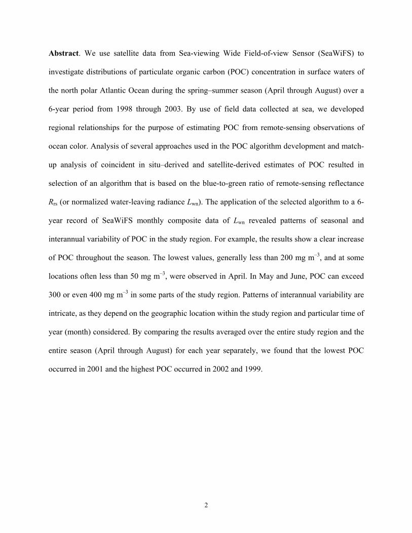
between 70ºN and 80ºN within the meridional zone between 1ºE and 20ºE (see Stramska et al.

[2003] for locations of stations). Figure 1 shows the locations of stations on R/V Polarstern. The

study region covered by the cruises includes waters of the Norwegian Sea, the confluence zone

of the Norwegian Sea and Barents Sea, the West Spitsbergen Current, and the Greenland Sea.

2.1.1. Water Sample Analyses

Suspended particles for the analysis of POC and Chl were collected by filtration of water

samples onto Whatman glass fiber filters (GF/F) under low vacuum. The POC samples were

collected on precombusted filters, dried at 55ºC, and stored until postcruise analysis in the

laboratory. POC was determined by combustion of sample filters [Parsons et al., 1984]. Before

this analysis, for removal of inorganic carbon, 0.25 mL of 10% HCl was applied to each sample

filter and the acid-treated filters were dried at 55ºC. During the cruises on R/V Oceania

relatively few samples for POC analysis were collected. The POC data from R/V Oceania will

not be used in the development of POC algorithms (but optical data collected on R/V Oceania

will be used in the algorithm development as described below). However, five POC

5

measurements from R/V Oceania will be used in the match-up comparisons of coincident in

situ–derived POC and satellite-derived POC with the purpose of validating the POC algorithms.

The POC data obtained on the R/V Polarstern cruise will be used in the POC algorithm

development. In total seventy seven POC estimates obtained on R/V Polarstern within the top

well-mixed layer of surface ocean (depths ≤ 50 m) are used in this study. Replicate samples for

POC determinations were usually taken and these determinations were averaged for final use.

In this paper we use the chlorophyll a concentration (Chl) determined by high-performance

liquid chromatography (HPLC) [Bidigare and Trees, 2000] for samples that were collected on

the R/V Polarstern cruise and stored in liquid nitrogen until postcruise analysis. Chl was

calculated as a sum of chlorophyll a and derivatives (chlorophyllide a, chlorophyll a allomers

and epimers). POC and Chl determined from the above-described analyses of discrete water

samples are referred to as in situ POC and in situ Chl estimates.

2.1.2. Optical Profiles

The time difference between the collection of water samples and acquisition of in situ optical

data was usually less than an hour. Detailed description of underwater optical measurements is

given elsewhere [Stramska et al., 2003] and the methodology of these measurements is

consistent with the SeaWiFS protocols [Mueller and Austin, 1995; Mueller, 2003]. Among the

various quantities measured, included were the underwater vertical profiles of downwelling

irradiance, Ed(z, λ), and upwelling radiance, Lu(z, λ), where z is depth and λ is wavelength of

light in vacuum. These radiometric measurements were made with a freefall spectroradiometer

(SPMR, Satlantic, Inc.) away from ship perturbations. Most of these measurements (~80%) were

made under cloudy skies and solar zenith angle between 47º and 65º. From the profiles of Ed(z,

6

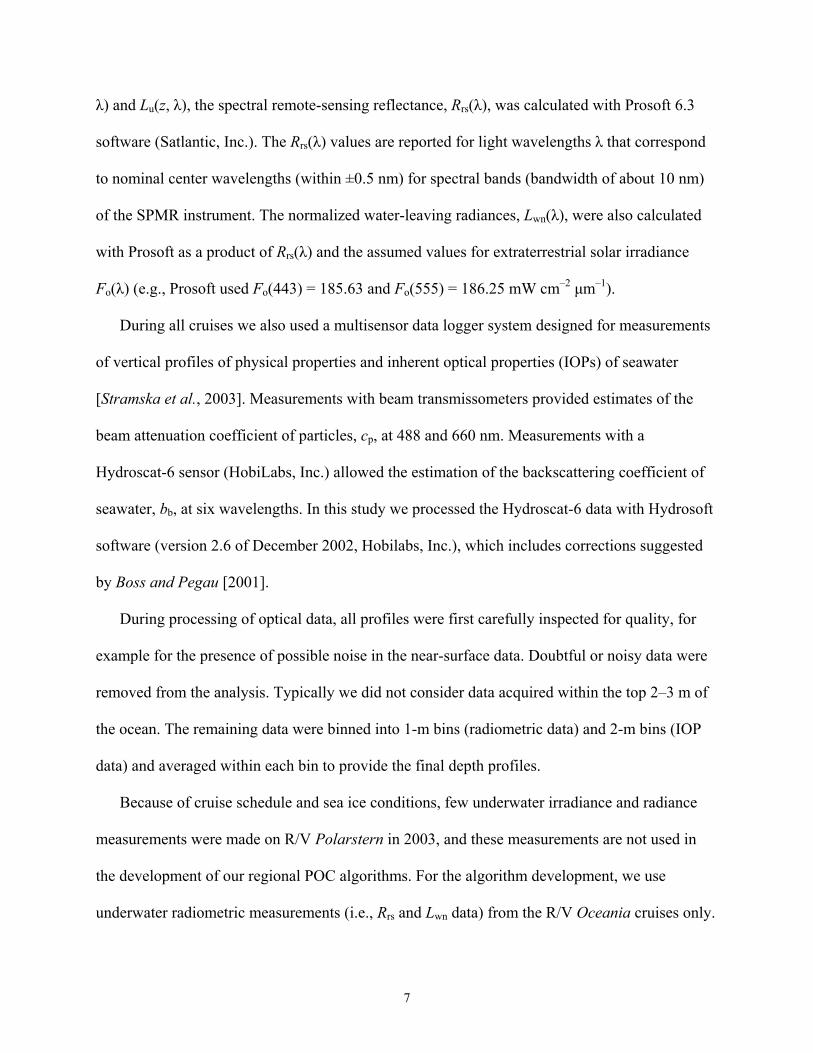
λ) and Lu(z, λ), the spectral remote-sensing reflectance, Rrs(λ), was calculated with Prosoft 6.3

software (Satlantic, Inc.). The Rrs(λ) values are reported for light wavelengths λ that correspond

to nominal center wavelengths (within ±0.5 nm) for spectral bands (bandwidth of about 10 nm)

of the SPMR instrument. The normalized water-leaving radiances, Lwn(λ), were also calculated

with Prosoft as a product of Rrs(λ) and the assumed values for extraterrestrial solar irradiance

Fo(λ) (e.g., Prosoft used Fo(443) = 185.63 and Fo(555) = 186.25 mW cm–2 µm–1).

During all cruises we also used a multisensor data logger system designed for measurements

of vertical profiles of physical properties and inherent optical properties (IOPs) of seawater

[Stramska et al., 2003]. Measurements with beam transmissometers provided estimates of the

beam attenuation coefficient of particles, cp, at 488 and 660 nm. Measurements with a

Hydroscat-6 sensor (HobiLabs, Inc.) allowed the estimation of the backscattering coefficient of

seawater, bb, at six wavelengths. In this study we processed the Hydroscat-6 data with Hydrosoft

software (version 2.6 of December 2002, Hobilabs, Inc.), which includes corrections suggested

by Boss and Pegau [2001].

During processing of optical data, all profiles were first carefully inspected for quality, for

example for the presence of possible noise in the near-surface data. Doubtful or noisy data were

removed from the analysis. Typically we did not consider data acquired within the top 2–3 m of

the ocean. The remaining data were binned into 1-m bins (radiometric data) and 2-m bins (IOP

data) and averaged within each bin to provide the final depth profiles.

Because of cruise schedule and sea ice conditions, few underwater irradiance and radiance

measurements were made on R/V Polarstern in 2003, and these measurements are not used in

the development of our regional POC algorithms. For the algorithm development, we use

underwater radiometric measurements (i.e., Rrs and Lwn data) from the R/V Oceania cruises only.

7

The IOP data (i.e., cp and bb) used in the algorithm development are from both R/V Oceania and

R/V Polarstern. As mentioned above, the POC data used in the algorithm development are from

R/V Polarstern only.

2.2. Satellite Data

The POC algorithms were applied to satellite data collected with the SeaWiFS instrument

over a period of 6 years from 1998 through 2003. These data were obtained from the NASA

Goddard Earth Sciences Data and Information Services Center (DAAC). The SeaWiFS provides

global coverage of water-leaving radiance at eight spectral bands in the visible and near-infrared

spectral region approximately every two days [e.g., Hooker and McClain, 2000]. To estimate

water-leaving radiances, the standard data processing procedures at NASA involve atmospheric

correction and removal of pixels with land, ice, clouds, and heavy aerosol load [e.g., Gordon and

Wang, 1994]. The standard data product of surface chlorophyll a concentration is determined

from satellite-derived water-leaving radiances using the empirical algorithm OC4v4 [O’Reilly et

al., 1998; 2000].

Our analysis of POC in the north polar Atlantic utilizes level 3 binned monthly SeaWiFS

data products of normalized water-leaving radiances Lwn(λ) and surface chlorophyll a

concentration, where each bin corresponds to a surface grid cell of approximately 81 square

kilometers in size (reprocessing version 4). The data cover the north polar Atlantic between

70ºN–80ºN and 11ºE–11ºW. For each year from 1998 through 2003, monthly composites for the

spring–summer season from April through August were selected for the analysis. The loss of

satellite data due to cloud cover often limits the availability of daily or 8-day composite

SeaWiFS data products; hence we use the monthly composites. For the remaining portion of the

8

year, there is no satellite data or there is insufficient amount of data in the study region because

of sea ice, cloudy skies, or the lack of daylight. As our interest is focused on large-scale patterns,

final satellite-derived results that illustrate the surface POC distributions in the study region are

binned to 1º x 1º grid to filter out the smaller-scale variability.

We note that although SeaWiFS data are acquired near local noon, in polar regions this is

always done at a relatively high solar zenith angle (SZA). For example, in our study region at

75ºN, SZA ranges at noon from about 65º in mid-April to 51.5º in mid-June. The low solar

elevations at high latitudes pose particular challenges for accurate remote sensing, which are

associated primarily with relatively low levels of water-leaving radiance (i.e., low ocean color

signal) and relatively long path lengths of solar photons in the atmosphere (i.e., high atmospheric

'noise'). These challenges underscore a need for validating ocean color algorithms by means of

comparison of coincident in situ data and satellite-derived data products. For validating our POC

algorithms, we compare coincident in situ POC estimates and satellite-derived POC estimates

from HRTP SeaWiFS data (i.e., high spatial resolution SeaWiFS data of about 1.1 km at nadir)

obtained under cloud-free skies on the same day and at the same geographical location as in situ

POC determinations. The pixels with the HRPT data included the position of ship station. The

time difference between the HRPT SeaWiFS data and in situ observations was less than 6 hours.

In some cases not one but two SeaWiFS overpasses during the same day were matched with one

in situ measurement.

3. POC Algorithms

3.1. Background

9

Stramski et al. [1999] showed that POC concentration in the surface ocean can be estimated

from satellite ocean color imagery. Their algorithm involved two empirical relationships derived

from field data collected in the Southern Ocean. One relationship links the surface POC with the

optical backscattering coefficient by particles, bbp. The other relationship links the remote-

sensing reflectance, Rrs, with the backscattering coefficient of seawater, bb = bbw + bbp (where bbw

is the backscattering coefficient of pure seawater). When the algorithm was applied to remotely

sensed data, bb (and hence bbp) was calculated first from satellite-derived Rrs, and then POC was

calculated from bbp. Both optical quantities involved in the algorithm were measured in the green

spectral region. This was justified by an intent to minimize the effect of the absorption

coefficient of seawater, a, on the algorithm performance. In the green spectral region, a is

expected to exhibit a relatively smaller change than bb if waters with a wide range of POC are

considered. We note that the use of absolute magnitude of satellite-derived Rrs at a single wave

band makes this algorithm particularly sensitive to potential errors in atmospheric correction.

However, the algorithm possesses a conceptual strength that stems from a two-step approach, in

which the constituent concentration is related to the inherent optical property (IOP) of seawater

(here POC and bbp, respectively) and the apparent optical property (AOP) of the ocean is related

to IOP of seawater (here Rrs and bb, respectively).

The relationships involved in the Stramski et al. [1999] algorithm have theoretical, albeit

somewhat confounded, basis. The relationships between Rrs and IOPs have been thoroughly

examined in the past. One important approach has been based on radiative transfer modeling,

which showed that Rrs is, to first approximation, proportional to bb and inversely proportional to

a [Gordon et al., 1975; Gordon and Morel, 1983; Kirk, 1984; Morel and Prieur, 1977]. The

coefficient of proportionality is not constant, however. It depends on water optical properties and

10

light conditions at the sea surface [Bukata et al., 1994; Kirk, 1991; Morel and Gentili 1991,

1993]. These effects, including the influence of absorption on Rrs, confound the direct relation

between Rrs and bb. Therefore no universal relationship between Rrs and bb is expected to hold

over a wide range of water bodies and light conditions. Nevertheless, Stramski et al. [1999]

showed a consistency in the Rrs versus bb relationship in the green band for two different water

bodies within the Southern Ocean; the Ross Sea and the Antarctic Polar Front Zone (APFZ).

Some basis for the relationship between POC and light scattering exists at the level of both

the bulk (volume) properties and the individual particles. At the level of individual particles,

carbon content of planktonic cells was shown to be coupled with particle size [Verity et al., 1992;

Montagnes et al., 1994] and refractive index [Stramski, 1999; DuRand et al., 2002]. Because

particle size and refractive index are primary determinants of particle scattering, there exists

linkage between carbon content and scattering of individual particles. The bulk properties, POC

and bbp, depend not only on the single particle properties but also on particle concentrations in

water. Under simplistic scenario that relative composition of particulate matter in water remains

constant, both POC and bbp would change in proportion to varying concentration of POC-bearing

particles. The actual relationship between POC and bbp in the ocean will be, however, more

complex than that driven solely by the particle concentration effect. This is due to variations in

the distribution of POC among different particle types/sizes and variations in the particulate

composition accompanied by changes in particle size, shape, and refractive index distributions

that influence bbp. One can therefore expect that various water bodies will exhibit different

magnitude of backscattering per POC content in water. Stramski et al. [1999] observed that the

relation between POC and bbp differs in a systematic way between the geographic regions of the

Ross Sea and APFZ. As a result of this difference, their APFZ algorithm predicts lower values of

11

POC from Rrs than the Ross Sea algorithm (typically by a factor of 2–4). These results support

the use of a regional approach in which the world's oceans are partitioned into provinces, within

which certain characteristic parameters or relationships can be assumed quasi-constant, at least

during a particular season [Platt and Sathyendranath, 1988; Mueller and Lange, 1989].

Because of the first-order effect of particle concentration on the bulk scattering of seawater,

bbp is expected to covary with the total particulate scattering coefficient, bp, and the particulate

beam attenuation coefficient, cp (especially in the spectral regions where particulate absorption is

weak). Therefore it is not surprising that data collected in different parts of the world’s ocean

show some (often significant) degree of correlation between cp or bp and POC [e.g., Gardner et

al., 1993; Marra et al., 1995; Loisel and Morel, 1998]. Such relationships were also supported

by laboratory experiments with phytoplankton cultures [e.g., Stramski and Morel, 1990; Stramski

and Reynolds, 1993]. These results open up a possibility that POC algorithms can be

alternatively developed with the POC versus cp or versus bp relationships. Because cp has been

routinely measured with in situ beam transmissometers for many years, it seems useful to

explore this option.

Recent attempt in this direction is described by Mishonov et al. [2003]. Their method is

based on two relationships. One relationship is between field measurements of cp(660) in the

South Atlantic and satellite (SeaWiFS) ocean color data products collected in the same region

over the same season (austral summer) but a decade later. The second relationship is between

POC and cp(660) established independently from field measurements in the North Atlantic. In

the final algorithm, POC calculated from cp(660) is linked to the satellite ocean color data

product. The SeaWiFS data product that provided the highest correlation with POC calculated

from cp(660), was the normalized water-leaving radiance in the green spectral band, Lwn(555).

12

Other products tested, the surface chlorophyll concentration, chlorophyll integrated over the first

attenuation depth, and diffuse attenuation coefficient for downward irradiance at 490 nm,

showed lower correlation. Mishonov et al. used the algorithm based on Lwn(555) in conjunction

with SeaWiFS imagery for illustrating POC distributions in the South Atlantic.

3.2. Regional POC Algorithms for the North Polar Atlantic

For the development of POC algorithms for the north polar Atlantic we evaluated the

following relationships: POC versus Chl, POC versus bb(589), POC versus cp(660), bb(589)

versus Rrs(555), and cp(660) versus Rrs(443)/Rrs(555) (and alternatively cp(660) versus

Lwn(443)/Lwn(555)). The relationships between POC versus bb(589) and POC versus cp(660)

were obtained by matching POC estimates from discrete water samples collected at a given depth

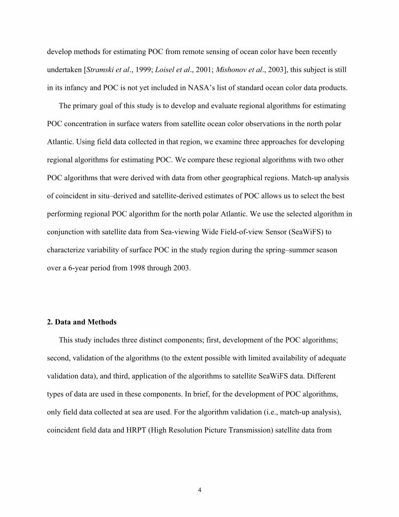
and the IOPs measured within a 2-m bin that corresponds to the depth of POC sample. Figure 2

shows example profiles of cp(660) and the corresponding POC values determined at discrete

depths. The thickness of surface layer that was relatively well mixed was determined from

inspection of each profile. Only the data collected within this surface layer were used to establish

the relationships between POC and IOPs. Most of these data were collected at depths between

the surface and 25 m. We did not use data from depths below 50 m and only 15–20% of data

included in the relationships between POC and IOPs come from depths ≥ 30 m. With regard to

the relationships bb(589) versus Rrs(555) and cp(660) versus Rrs(443)/Rrs(555) (or cp(660) versus

Lwn(443)/Lwn(555)), we used the bb(589) and cp(660) values averaged between the depths of 3

and 5 m and the Rrs(λ) or Lwn(λ) values estimated from concurrent measurements of underwater

radiometric profiles.

13

3.2.1. Algorithm 1

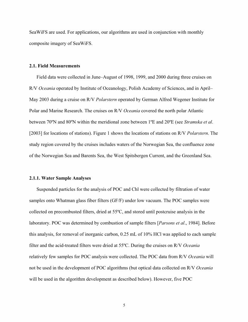
Our first algorithm (referred to as algorithm 1) consists of two relationships, namely cp(660)

versus Rrs(443)/Rrs(555) and POC versus cp(660). Alternatively, the first relationship of this

algorithm is based on Lwn(443)/Lwn(555) instead of Rrs(443)/Rrs(555) (Table 1). The relationship

between cp(660) and Lwn(443)/Lwn(555) is shown in Figure 3a. This relationship was determined

from in-water optical data collected on R/V Oceania in 1998, 1999, and 2000. The POC versus

cp(660) relationship was determined from field data collected on R/V Polarstern in 2003 (Figure

3b). This relationship is compared with similar relationships established previously in other

oceanic regions (Figure 3c). When applied to remotely sensed data, algorithm 1 operates in such

a way that cp(660) is derived first from the satellite-derived blue-to-green ratio of Rrs or Lwn.

Then the POC versus cp(660) relationship is used to estimate surface POC concentration.

The main reason for using cp(660) in algorithm 1 is the availability of data sets that were

collected concurrently. Specifically, whereas a relatively large set of POC and IOP data but few

underwater radiometric data were collected on R/V Polarstern, a substantial set of IOP and

radiometric data with few POC data were collected on the R/V Oceania cruises. This situation

resulted from differences in research goals and logistics of the cruises, sea ice conditions, and

episodes of malfunctioning of different instruments. Had we have available a sufficiently large

set of concurrent measurements of POC and Rrs or Lwn band ratios, algorithm 1 would have been

developed in terms of a direct relation between these variables without use of cp(660). We also

note that our data suggest that the use of 490 nm and 555 nm (not shown here) would be at least

as good as 443 nm and 555 nm for this type of band ratio algorithm. However, the number of our

radiometric data at 490 nm is limited because the SPMR spectroradiometer experienced a failure

14

at 490 nm spectral channel during a significant portion of our cruises. Hence we use 443 nm in

our algorithm 1.

Although algorithm 1 involves cp(660), it is conceptually different from that of Mishonov et

al. [2003], because we use the spectral ratio of Lwn rather than Lwn at a single wavelength. It is

also important to realize that our algorithm 1 could be viewed simply as a one-step algorithm

based on a relationship between the blue-to-green ratio of Lwn and POC. This is because there

seems to be no profound basis for the relationship between Lwn(443)/Lwn(555) and cp(660), so

here the role of cp(660) is merely to provide an intermediate proxy for POC. As mentioned

above, we did not establish the direct relationship between Lwn (or Rrs) band ratio and POC from

our cruises because we did not have a large enough number of concurrent underwater

radiometric and POC data. Such a direct relationship forms, however, a basis of algorithm 4 that

is derived from historical data from other geographic regions (see discussion below).

By linking POC to the blue-to-green ratio of Lwn or Rrs, algorithms 1 and 4 are conceptually

similar to the common approach that has been used in the empirical chlorophyll algorithms for

many years [e.g., O’Reilly et al., 1998; 2000]. In the case of chlorophyll, this approach relies on

variations in the reflectance ratio, which are driven largely by changes in the absorption

coefficient of seawater associated with varying concentration of pigment-containing

phytoplankton. In the case of POC, this type of algorithm also takes advantage of variations in

the absorption coefficient that is associated with all kinds of POC-containing particles, including

detritus and heterotrophic organisms in addition to phytoplankton. Because the absorption

coefficients of all POC particle types are expected to show an increase from the green toward the

blue spectral region, all these particle types are also expected, at least to first approximation, to

exert a qualitatively similar effect on the blue-to-green ratio of normalized water-leaving

15

radiance or ocean reflectance. This is essentially a basis for our regional algorithm 1 (as well as

algorithm 4 described below).

3.2.2. Algorithm 2

The second regional POC algorithm (referred to as algorithm 2) is a two-step approach, in

which the IOP is linked to POC and the AOP is linked to the IOP (Table 1). The IOP is the

backscattering coefficient at 589 nm, bb(589). The AOP is the remote-sensing reflectance at 555

nm, Rrs(555) (or alternatively Lwn(555). Both relationships have been selected on the same

theoretical grounds as discussed above with regard to the Stramski et al. [1999] algorithm. When

applied to remotely sensed data from satellite observations, algorithm 2 operates in such a way

that bb(589) is first calculated from the satellite-derived Rrs(555) or Lwn(555) and then POC is

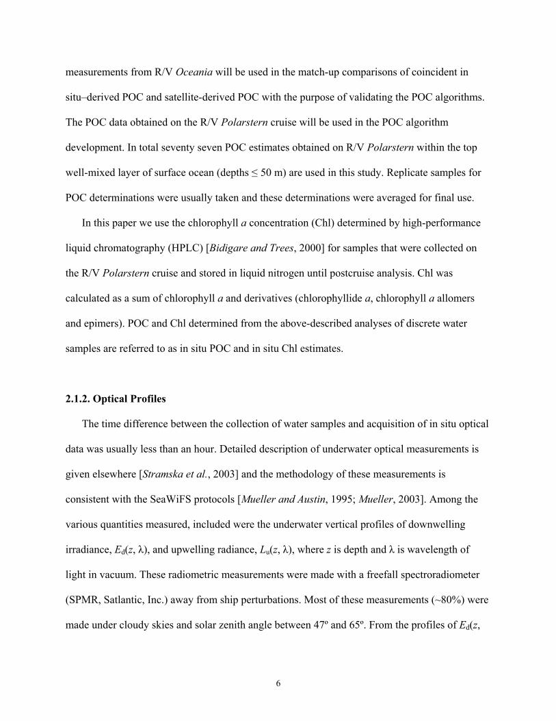
calculated from bb(589). The relationship between bb(589) and Rrs(555) was established from our

in-water optical measurements made in 1998, 1999, and 2000 on R/V Oceania, whereas the

relationship between POC and bb(589) was derived from the POC and bb(589) measurements

made in 2003 on R/V Polarstern (Figure 4). Note that the extrapolation of the regression formula

describing POC versus bb(589) to POC = 0 yields bb(589) of 0.00767 m–1, which is very close to

the theoretical value of 0.0075 m–1 for pure seawater backscattering at 589 nm [e.g., Smith and

Baker, 1981].

Although algorithm 2 is conceptually similar to that of Stramski et al. [1999], there are a few

slight differences. Here we use the total backscattering coefficient in both steps of the algorithm,

whereas Stramski et al. used the particulate backscattering in the step that links backscattering

with POC. Second, we use bb at 589 nm because during our cruises the Hydroscat-6 instrument

experienced no failure in this spectral band and because this band still represents the middle

16

portion of visible spectrum with relatively small variations in absorption. In the north polar

Atlantic we collected more bb data of good quality at 589 nm than at 555 nm. Stramski et al. used

bbp at 510 nm because this channel provided data of consistently good quality on their cruises in

the Southern Ocean and their Hydroscat-6 was not equipped with a 555-nm channel.

Importantly, both algorithms use the wave bands in the green spectral region, where large

changes in POC are accompanied by relatively large changes in bb and relatively smaller changes

in the absorption coefficient. Hence a reasonably good relationship is anticipated between Rrs (or

Lwn) and POC calculated from bb or bbp.

3.2.3. Algorithm 3

Although the POC/Chl ratio can vary over broad range in the ocean [e.g., Chung et al.,

1996], these variables may often show a significant correlation, especially if the data are

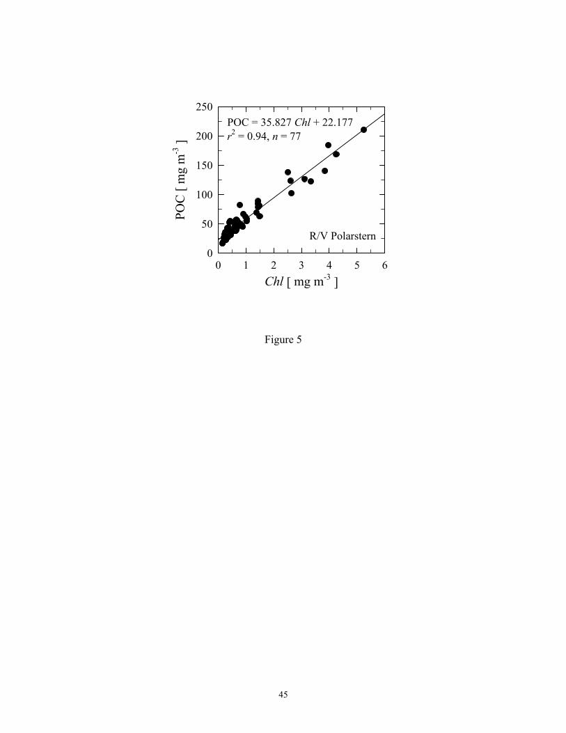
regionally and seasonally constrained. Our third regional POC algorithm (referred to as

algorithm 3), is described by a relationship between POC and Chl obtained from measurements

on the R/V Polarstern cruise (Figure 5 and Table 1). We note that our POC and Chl data suggest

that waters examined during that cruise were characterized by a relatively low POC at any given

Chl value. During the summer cruises on R/V Oceania, we generally observed higher values of

POC at given Chl values (not shown). In remote-sensing applications, the input to algorithm 3 is

the NASA's standard satellite-derived global data product of surface chlorophyll a concentration

(currently estimated from the OC4 algorithm).

It is important to note that our regional algorithms were developed with data from open

ocean waters where organic carbon-containing particles of biological origin usually dominate the

particulate optical properties [e.g., Morel and Prieur, 1977; Smith and Baker, 1978]. In waters

17

that are optically more complex (e.g., Spitsbergen coastal region characterized by glacial

discharge of minerogenic particulate matter), our algorithms may be subject to large error. This

source of error is well known for the Chl algorithms [e.g., Woźniak and Stramski, 2004] and it is

also expected in the POC algorithms.

3.3. Other POC Algorithms

The match-up data set for validating our regional POC algorithms, that is, for comparing

coincident in situ estimates of POC and satellite-derived estimates of POC based on cloud-free

HRPT imagery from SeaWiFS, is small for our cruises in the north polar Atlantic (see Section

4.2 below). This is largely caused by predominantly cloudy skies during the cruises. To provide

an additional means for testing our regional algorithms, the POC estimates from these regional

algorithms will be compared with POC estimates obtained from two other algorithms that are

based on data from other geographical regions. These two algorithms are described below.

The POC algorithm 4 is a correlational algorithm similar to common algorithms for

estimating global distributions of surface Chl from ocean color measurements. In such

algorithms the blue-to-green ratio of Rrs or Lwn is used to calculate Chl [e.g., O’Reilly et al.,

1998, 2000]. Our algorithm 4 is based on the relationship between surface POC concentration

and remote-sensing reflectance ratio Rrs(443)/Rrs(555) [or Rrs(490)/Rrs(555)] established from

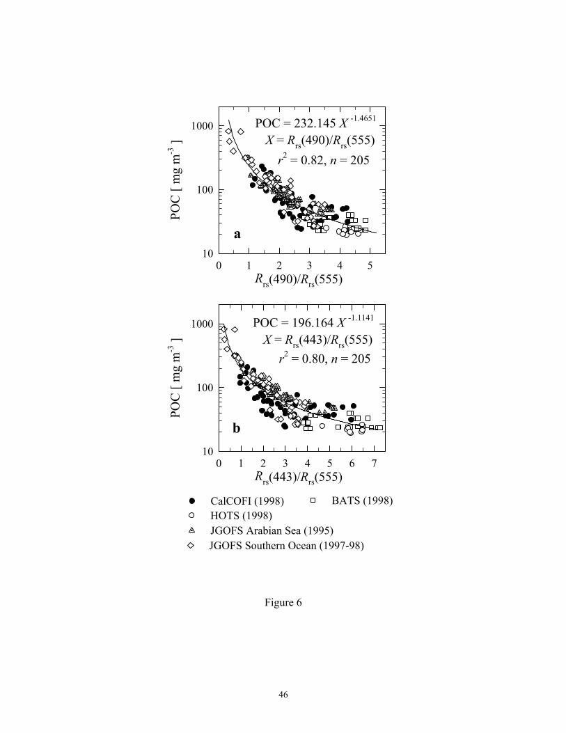
field data collected in various geographical regions of the world's ocean (Figure 6 and Table 1).

The data presented in Figure 6 were obtained from the public databases of U.S. Joint Global

Ocean Flux Study (JGOFS) and the NASA Sensor Intercomparison for Marine Biological and

Interdisciplinary Ocean Studies (SIMBIOS). Specifically, we selected some data from the

following field projects: CalCOFI in waters off California, BATS near Bermuda Islands in the

18

subtropical north Atlantic, HOTS near Hawaii in the North Pacific, JGOFS in the Arabian Sea,

and JGOFS in the Southern Ocean. For this data set, both reflectance ratios perform similarly in

terms of POC prediction. For our further analysis we choose Rrs(443)/Rrs(555).

Finally, we test the POC algorithm 5 that estimates POC from Lwn(555) (Table 1). This

algorithm was developed for the austral summer season in the South Atlantic by Mishonov et al.

[2003] as already briefly described in section 3.1.

4. Results and Discussion

In section 4.1 we compare the POC estimates 1–5 obtained by application of algorithms 1–5

to the same set of SeaWiFS data. In section 4.2 we present match-up comparisons of the satellite-

derived POC based on HRPT SeaWiFS imagery with available coincident in situ data of POC. In

section 4.3 we demonstrate the POC variability in the study region over a 6-year period on the

basis of the application of our algorithm 1 to SeaWiFS monthly composite imagery. In the

description below the term ‘monthly POC’ (or, for example, ‘April POC’) refers to the POC

concentration in surface waters estimated from a monthly (for example, April) composite of

SeaWiFS data. The term ‘seasonal POC’ refers to an average of five monthly POC estimates

(April through August). The term POC estimate 1 refers to POC estimated from algorithm 1,

POC estimate 2 refers to POC estimated from algorithm 2, etc.

4.1. Comparison of POC Estimates From Different Algorithms

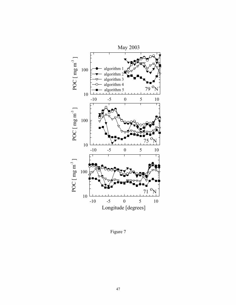
Figure 7 compares the POC estimates from the five algorithms whose input is the SeaWiFS

monthly composite data for May 2003 at transects along 71º, 75º and 79ºN in the north polar

Atlantic. The POC algorithms vary widely in the prediction of POC concentration. The regional

19

algorithm 1 for the north polar Atlantic and algorithm 4 produce consistently similar estimates of

POC for all the data presented. This consistency is remarkable given that algorithm 4 is based on

data from several regions far from the north polar Atlantic. The POC concentrations derived

directly from the SeaWiFS Chl using the regional algorithm 3 are consistently and significantly

lower than the POC estimates 1 and 4. Because this result is for May 2003 when the in situ POC

and Chl data were actually collected for the development of algorithm 3, it seems unlikely that

these differences between algorithm 3 and algorithms 1 and 4 in Figure 7 are caused by highly

inadequate relationship between in situ POC and in situ Chl. The presence of systematic error in

the satellite Chl derived from the current NASA global chlorophyll algorithm in the north polar

Atlantic [Stramska et al., 2003] may be, at least partly, responsible for the differences.

The regional algorithm 2 exhibits variable behavior when compared to the prediction of

algorithms 1 and 4 (Figure 7). There is a good agreement between algorithms 1, 2, and 4 for

most data points along the 71ºN transect (with the exception of the section between 4ºW and

7ºW). The eastern and western parts of the 75ºN transect also show good agreement between the

three algorithms. The major discrepancies are observed along 75ºN between 1ºE and 6ºW where

the POC estimate 2 is significantly lower (occasionally more than 10 times) than the POC

estimates 1 and 4. This tendency for producing lower POC values is also clearly seen for most

data points that represent algorithm 2 along 79ºN. In a few extreme cases, the POC estimates 2

assumed unrealistic (negative) values at 75ºN. This may be indicative of large error in the

retrieval of Lwn(555) and Rrs(555) from SeaWiFS data rather than such a large problem in the in-

water relationships defining algorithm 2. Algorithm 2 is based on a single wave band so it

depends critically on the accuracy of the estimation of absolute magnitude of satellite-derived

20

Lwn(555) and Rrs(555). Hence this algorithm is particularly sensitive to atmospheric correction

and other error sources in the satellite-derived water-leaving radiance.

Algorithm 5 consistently shows large underprediction of POC compared to algorithms 1 and

4 (Figure 7). Because both algorithm 2 and algorithm 5 use essentially the same SeaWiFS data

product, Lwn(555), for determining POC, the coincidence of very low estimates 2 and 5 over

some portions of the 75ºN and 71ºN transects supports the notion that the satellite-derived

Lwn(555) could be in large error in those particular areas. We note, however, that the POC

estimates 5 are generally quite different than those from our regional algorithm 2. Whereas

algorithm 2 often produces POC that is consistent with algorithms 1 and 4, algorithm 5 always

produces lower estimates. The consistently different performance of algorithm 5 is probably

partly attributable to the fact that it is based on data from other geographical regions. It is likely,

however, that part of the problem is associated also with an approach used in the development of

algorithm 5 by Mishonov et al. [2003]. In particular, their algorithm has not been developed by

use of concurrently collected field data. Algorithm 5 is based on relationships between

seasonally averaged parameters from different regions and years. We omit this algorithm from

further discussion.

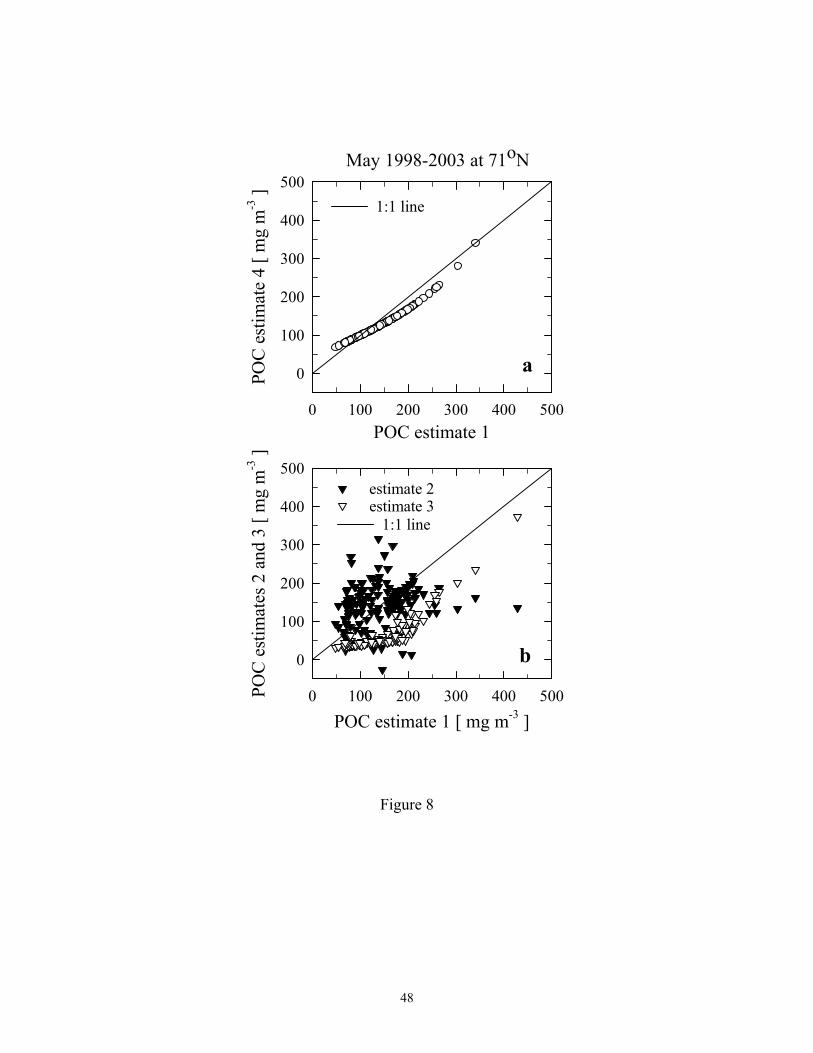
Additional insight into the differences between the POC estimates from the different

algorithms is provided in Figure 8. The POC estimates 2, 3, and 4 are plotted against the estimate

1. These results include the data from the month of May from the 6-year period along the 71ºN

transect but they are fairly typical for the entire data set examined in this study. Although a small

systematic difference occurs between the POC estimates 1 and 4, Figure 8a reveals a good

correlation between these estimates. It is also seen that algorithm 3 produces systematically low

POC (Figure 8b). Finally, we see that algorithm 2 is erratic in the sense that the POC estimates

21

show large scatter (Figure 8b). We believe that this large scatter results, at least partly, from

higher sensitivity of algorithm 2 to errors in satellite retrievals of water-leaving radiance at 555

nm compared to algorithms 1, 3, and 4, which are all based on the band ratios of satellite-derived

Lwn or Rrs.

4.2. Validation of POC Algorithms

The validation of ocean color algorithms can be based on a comparison of coincident remote-

sensing data products and in situ data. Such comparison is often referred to as a match-up

analysis. Unfortunately very few in situ POC data concurrent with HRPT SeaWiFS data are

presently available in the north polar Atlantic for validating our POC algorithms. Figure 9a

compares the few in situ POC estimates with the POC estimates obtained from the concurrent

satellite measurements (i.e., SeaWiFS-derived Lwn) using algorithms 1 and 4. The field data

considered were collected in 1998 and 1999 on R/V Oceania and they were not used in the

development of algorithms. Although the number of match-up data points is small, the satellite-

derived POC from algorithm 1 agrees quite well with the in situ POC. This result supports the

feasibility of estimating POC from algorithm 1 in the study region. The algorithm 4–derived

POC in the north polar Atlantic is generally lower than the in situ POC (Figure 9a). This is

consistent with Figure 8a.

Figure 9b shows similar validation results but the algorithm 4–derived POC from HRPT

SeaWiFS measurements is compared with concurrent in situ POC found in historical data

collected in various oceanic regions, including those used in the development of algorithm 4.

Although there is scatter in the data points, algorithm 4 frequently produces reasonably good

22

estimates of POC. Overall there is no clear systematic deviation between the algorithm 4–derived

POC and in situ POC in this match-up analysis.

Although the match-up analysis cannot be perfect in terms of spatial, temporal, and spectral

matching of satellite and in situ observations, the validation results such as those presented in

Figure 9 allow us to estimate the final errors in satellite-derived data products. In addition to

issues associated with imperfect spatial, temporal, and spectral matching, the final errors implied

by the match-up analysis are affected by various other sources including imperfect radiometric

calibration of instruments, atmospheric correction, in-water algorithm, effects of solar angle and

sensor viewing geometry, etc. The mean normalized bias (MNB) and the normalized root mean

square (RMS) error [e.g., Darecki and Stramski, 2004] for algorithm 4 and the data shown in

Figure 9b are 2.7% and 35.8%, respectively. For the small number of data points from the north

polar Atlantic in Figure 9a, MNB = –12% and RMS = 15.9% for our regional algorithm 1, and

MNB = –34.5% and RMS = 6.5% for algorithm 4. Despite the small number of validation data

points, Figure 9a suggests that a regional algorithm 1 can perform well in the north polar

Atlantic. For illustrating seasonal and interannual variability in POC over a 6-year period in the

study region (section 4.3 below), we selected algorithm 1 as the best choice among the regional

algorithms examined.

Because errors in the retrieval of Lwn from satellite signal (caused, for example, by

atmospheric correction) propagate into the estimation of POC, it is also instructive to recall

results of match-up analysis for Lwn in our study region [Stramska et al., 2003]. This analysis

was based on 13 match-up observations and it showed a relatively good agreement between the

satellite-derived and in situ values of the band ratio Lwn(490)/Lwn(555). The satellite-derived ratio

was, on average, 6% higher than the in situ ratio. As could have been expected, the agreement

23

was not as good for Lwn at single wavelengths. For example, at 555 nm the satellite-derived Lwn

was, on average, 14% lower than its in situ counterpart.

4.3. Variability in Surface POC in the North Polar Atlantic

Using algorithm 1 in conjunction with SeaWiFS imagery from the region of north polar

Atlantic (70ºN–80ºN and 11ºE–11ºW), we obtained monthly estimates (from April to August) of

surface POC for each year from 1998 to 2003. Figures 10, 11, 12, 13, and 14 present the results

for selected transects across the study region (71ºN, 75ºN, and 79ºN). The region is characterized

by a wide seasonal range of POC with high values occurring from May through the summer and

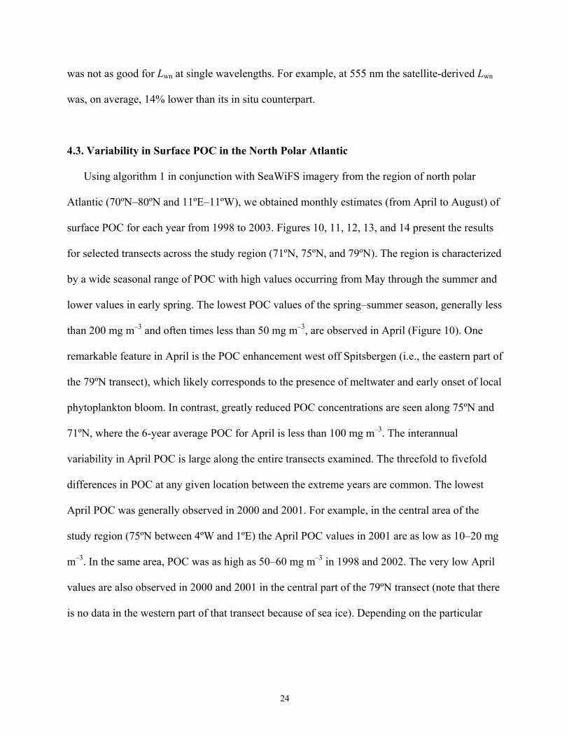
lower values in early spring. The lowest POC values of the spring–summer season, generally less

than 200 mg m–3 and often times less than 50 mg m–3, are observed in April (Figure 10). One

remarkable feature in April is the POC enhancement west off Spitsbergen (i.e., the eastern part of

the 79ºN transect), which likely corresponds to the presence of meltwater and early onset of local

phytoplankton bloom. In contrast, greatly reduced POC concentrations are seen along 75ºN and

71ºN, where the 6-year average POC for April is less than 100 mg m–3. The interannual

variability in April POC is large along the entire transects examined. The threefold to fivefold

differences in POC at any given location between the extreme years are common. The lowest

April POC was generally observed in 2000 and 2001. For example, in the central area of the

study region (75ºN between 4ºW and 1ºE) the April POC values in 2001 are as low as 10–20 mg

m–3. In the same area, POC was as high as 50–60 mg m–3 in 1998 and 2002. The very low April

values are also observed in 2000 and 2001 in the central part of the 79ºN transect (note that there

is no data in the western part of that transect because of sea ice). Depending on the particular

24

location within the study region, the highest April POC values occurred in different years (but

excluding 2000 and 2001).

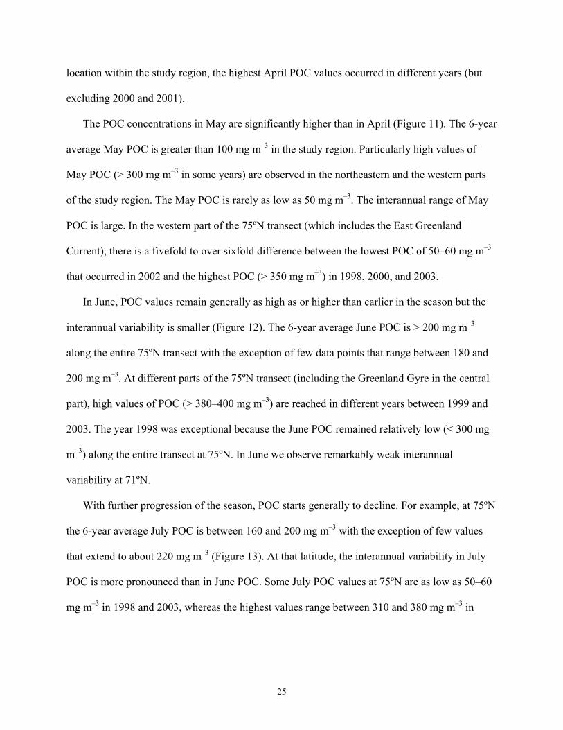
The POC concentrations in May are significantly higher than in April (Figure 11). The 6-year

average May POC is greater than 100 mg m–3 in the study region. Particularly high values of

May POC (> 300 mg m–3 in some years) are observed in the northeastern and the western parts

of the study region. The May POC is rarely as low as 50 mg m–3. The interannual range of May

POC is large. In the western part of the 75ºN transect (which includes the East Greenland

Current), there is a fivefold to over sixfold difference between the lowest POC of 50–60 mg m–3

that occurred in 2002 and the highest POC (> 350 mg m–3) in 1998, 2000, and 2003.

In June, POC values remain generally as high as or higher than earlier in the season but the

interannual variability is smaller (Figure 12). The 6-year average June POC is > 200 mg m–3

along the entire 75ºN transect with the exception of few data points that range between 180 and

200 mg m–3. At different parts of the 75ºN transect (including the Greenland Gyre in the central

part), high values of POC (> 380–400 mg m–3) are reached in different years between 1999 and

2003. The year 1998 was exceptional because the June POC remained relatively low (< 300 mg

m–3) along the entire transect at 75ºN. In June we observe remarkably weak interannual

variability at 71ºN.

With further progression of the season, POC starts generally to decline. For example, at 75ºN

the 6-year average July POC is between 160 and 200 mg m–3 with the exception of few values

that extend to about 220 mg m–3 (Figure 13). At that latitude, the interannual variability in July

POC is more pronounced than in June POC. Some July POC values at 75ºN are as low as 50–60

mg m–3 in 1998 and 2003, whereas the highest values range between 310 and 380 mg m–3 in

25

1999 (between 1ºW and 9ºW). Note that by July the sea ice in the northwestern part of the study

region decayed to the extent that we have satellite data available for that area.

Further decline, albeit not dramatic, in the 6-year average POC is observed in August for

most areas within the study region (Figure 14). Compared to the month of July, the interannual

variability in August POC significantly weakened in the western and central parts of the 75ºN

transect. However, in the eastern part of the transect the variability is large. At 71ºN the

interannual variability in the August POC shows some evidence of increase compared to July

and June. At 79ºN the interannual variability appears to have a comparable range throughout

much of the summer season.

It is important to note that the overall patterns of interannual variability of POC in the study

region are complex in the sense that local minimum (or maximum) POC values observed over

the 6-year period may correspond to different years depending on the month and location

considered. For example, in April the minimum values in different parts of the study region were

predominantly in the years 2000 or 2001. In June, however, the minimum values for many

locations were in the years 1998, 1999, or 2003. Because the patterns of interannual variability

are quite intricate depending not only on the geographic location but also on the particular time

(month) within the spring–summer season, it is useful to look at the interannual variability in

seasonally averaged POC. These seasonally averaged POC concentrations were calculated by

averaging five monthly (April through August) POC estimates for each year separately. In

addition, a 6-year average of seasonally averaged POC was estimated by averaging all the

seasonal estimates. We present these results in Figure 15 for latitudinal transects in 1 degree

increments from 70ºN to 79ºN. The variation in seasonal POC by a factor of 2 between the

extreme years is quite common across the study region. Sporadically, a threefold range is

26

observed, for example at 75ºN between 4ºE and 5ºE. The transects from the southern part of the

region generally show somewhat lower values of the 6-year average seasonal POC than other

areas. At these relatively low latitudes, the lowest seasonal POC values most commonly

correspond to the year 2001. This is not the case, however, at other latitudes. For example, at

76º–77ºN the lowest seasonal POC estimates were typically obtained in 1998. These results

show that it is difficult to reveal consistent or simple patterns with regard to which year produced

the lowest or highest seasonal POC within the study region.

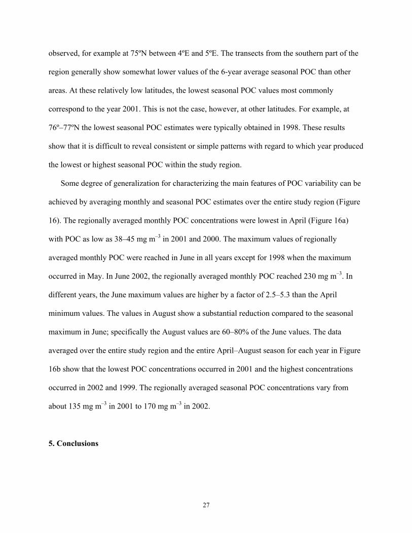
Some degree of generalization for characterizing the main features of POC variability can be

achieved by averaging monthly and seasonal POC estimates over the entire study region (Figure

16). The regionally averaged monthly POC concentrations were lowest in April (Figure 16a)

with POC as low as 38–45 mg m–3 in 2001 and 2000. The maximum values of regionally

averaged monthly POC were reached in June in all years except for 1998 when the maximum

occurred in May. In June 2002, the regionally averaged monthly POC reached 230 mg m–3. In

different years, the June maximum values are higher by a factor of 2.5–5.3 than the April

minimum values. The values in August show a substantial reduction compared to the seasonal

maximum in June; specifically the August values are 60–80% of the June values. The data

averaged over the entire study region and the entire April–August season for each year in Figure

16b show that the lowest POC concentrations occurred in 2001 and the highest concentrations

occurred in 2002 and 1999. The regionally averaged seasonal POC concentrations vary from

about 135 mg m–3 in 2001 to 170 mg m–3 in 2002.

5. Conclusions

27

This study is an extension of a few previous efforts toward estimating surface concentration

of POC from satellite ocean color observations [Stramski et al., 1999; Loisel et al., 2001, 2002;

Mishonov et al., 2003]. By demonstrating the feasibility of remote sensing of POC, these initial

studies pave the way for further research in this direction. Future success of this application of

ocean color observations will depend on the continued efforts to develop robust POC algorithms

and their rigorous validation. Here we used field data collected on four cruises and satellite

imagery obtained with SeaWiFS sensor in the north polar Atlantic in order to examine and

validate several approaches for estimating surface POC from observations of ocean color. Our

analysis suggests that a regional algorithm (referred to as algorithm 1) based on the blue-to-green

ratio of remote-sensing reflectance (or normalized water-leaving radiance) can be used to obtain

estimates of POC in the investigated region. Although few appropriate data are presently

available for validating the POC algorithms, the reasonably good agreement between satellite-

based determinations of POC derived from the band ratio algorithm 1 and coincident ship-based

determinations of surface POC is encouraging. We also found that the POC estimates from the

regional algorithm 1 were generally consistent with the POC estimates obtained from a similar

band ratio algorithm that was developed with independent historical field data collected in

various oceanic waters other than the north polar Atlantic.

The application of the regional algorithm 1 to a 6-year record of SeaWiFS data covering the

spring–summer seasons from 1998 to 2003 provided insight into the POC distributions and their

seasonal and interannual variability in the north polar Atlantic. The results show a clear increase

of POC throughout the season. The lowest values generally less than 200 mg m–3, and often

times less than 50 mg m–3 at some locations, were observed in April. In May and June, POC can

exceed 300 or even 400 mg m–3 in some parts of the study region. Patterns of interannual

28

variability are intricate as they depend on the geographical location within the study region and

particular time of year (month) considered. By comparing the results averaged over the entire

study region and the entire April–August season for each year separately, we found that the

lowest POC occurred in 2001 and the highest POC occurred in 2002 and 1999.

Acknowledgments. The analysis of the north polar Atlantic data was supported by NASA

grants NAG5-12396 and NAG5-12397, and the analysis of historical POC and optical data was

supported by NSF grants OCE-0324346 and OCE-0324680. The historical field data were

obtained from the U.S. JGOFS and SIMBIOS databases. The principal investigators who

provided those data are M. Abbott, W. Gardner, D. Karl, R. Letelier, G. Mitchell, F. Muller-

Karger, D. Siegel, and C. Trees. The SeaWiFS data were made available by NASA’s Goddard

Earth Sciences Data and Information Services Center (DAAC) and the SeaWiFS Science Project.

The Institute of Oceanology, Polish Academy of Sciences (Sopot, Poland) and the Alfred

Wegener Institute for Polar and Marine Research (Bremerhaven, Germany) made it kindly

possible for us to participate in the polar cruises on R/V Oceania and R/V Polarstern. We are

especially grateful to chief scientists J. Piechura, W. Walczowski, and G. Kattner for

accommodating our in situ optical deployments on their cruises. We thank the scientists, officers,

and crews of R/V Oceania and R/V Polarstern who provided logistical support and helped us in

the fieldwork. Our special thanks go to D. Allison, R. Hapter, S. Kaczmarek, T. Petelski, M.

Sokólski, J. Schwarz, and A. Stoń for assistance in the collection of field data for this study. The

HPLC analysis of pigment samples was made at the Center for Hydro-Optics and Remote

Sensing, San Diego State University. The analysis of samples for particulate organic carbon was

made at Marine Science Institute Analytical Laboratory, University of California, Santa Barbara.

29

References

Bidigare, R., and C. C. Trees (2000), HPLC phytoplankton pigments: Sampling, laboratory

methods, and quality procedures assurance, in Ocean Optics Protocols for Satellite Ocean

Color Sensor Validation, Revision 2, NASA/TM 2000-209966, edited by G.S. Fargion and

J.L. Mueller, pp. 154–161, NASA, Washington, D.C.

Boss, E., and W. S. Pegau (2001), The relationship of light scattering at an angle in the backward

direction to the backscattering coefficient, Appl. Opt., 40, 5503–5507.

Bukata, R. P., J. H. Jerome, K. J. Kondratyev, and D.V. Pozdnyakov (1994), Optical Properties

and Remote Sensing of Inland and Coastal Waters, 362 pp., CRC Press, Boca Raton, Fla.

Darecki, M., and D. Stramski (2004), An evaluation of MODIS and SeaWiFS bio-optical

algorithms in the Baltic Sea, Remote Sens. Environ., 89, 326–350.

DuRand, M. D., R. E. Green, H. M. Sosik, and R. J. Olson (2002), Diel variations in optical

properties of Micromonas pusilas (Prasinophyceae), J. Phycol., 38, 1132–1142.

Chung, S. P., W. D. Gardner, M. J. Richardson, I. D. Walsh, and M. R. Landry (1996), Beam

attenuation and microorganisms: Spatial and temporal variations in small particles along

140ºW during 1992 JGOFS-EqPac transect, Deep Sea Res., Part II, 43, 1205–1226.

Clarke, G. L., G. C. Ewing, and C. J. Lorenzen (1970), Spectra of backscattered light from the

sea obtained from aircraft as a measure of chlorophyll concentration, Science, 167, 1119–

1121.

Gardner, W. D., I. D. Walsh, and M. J. Richardson (1993), Biophysical forcing of particle

production and distribution during a spring bloom in the North Atlantic, Deep Sea Res., Part

II, 40, 171–195.

30

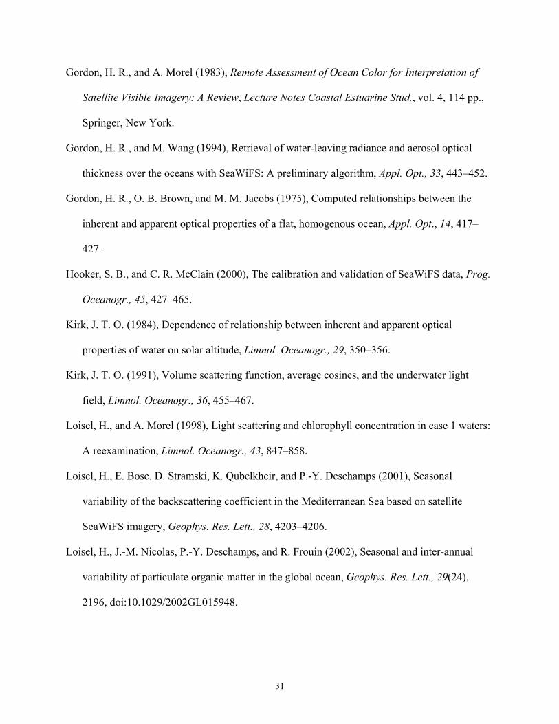
Gordon, H. R., and A. Morel (1983), Remote Assessment of Ocean Color for Interpretation of

Satellite Visible Imagery: A Review, Lecture Notes Coastal Estuarine Stud., vol. 4, 114 pp.,

Springer, New York.

Gordon, H. R., and M. Wang (1994), Retrieval of water-leaving radiance and aerosol optical

thickness over the oceans with SeaWiFS: A preliminary algorithm, Appl. Opt., 33, 443–452.

Gordon, H. R., O. B. Brown, and M. M. Jacobs (1975), Computed relationships between the

inherent and apparent optical properties of a flat, homogenous ocean, Appl. Opt., 14, 417–

427.

Hooker, S. B., and C. R. McClain (2000), The calibration and validation of SeaWiFS data, Prog.

Oceanogr., 45, 427–465.

Kirk, J. T. O. (1984), Dependence of relationship between inherent and apparent optical

properties of water on solar altitude, Limnol. Oceanogr., 29, 350–356.

Kirk, J. T. O. (1991), Volume scattering function, average cosines, and the underwater light

field, Limnol. Oceanogr., 36, 455–467.

Loisel, H., and A. Morel (1998), Light scattering and chlorophyll concentration in case 1 waters:

A reexamination, Limnol. Oceanogr., 43, 847–858.

Loisel, H., E. Bosc, D. Stramski, K. Qubelkheir, and P.-Y. Deschamps (2001), Seasonal

variability of the backscattering coefficient in the Mediterranean Sea based on satellite

SeaWiFS imagery, Geophys. Res. Lett., 28, 4203–4206.

Loisel, H., J.-M. Nicolas, P.-Y. Deschamps, and R. Frouin (2002), Seasonal and inter-annual

variability of particulate organic matter in the global ocean, Geophys. Res. Lett., 29(24),

2196, doi:10.1029/2002GL015948.

31

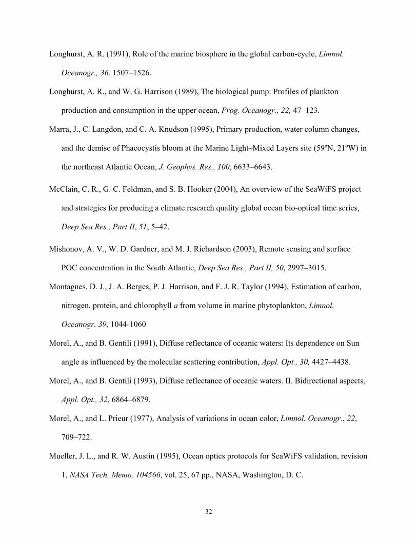
Longhurst, A. R. (1991), Role of the marine biosphere in the global carbon-cycle, Limnol.

Oceanogr., 36, 1507–1526.

Longhurst, A. R., and W. G. Harrison (1989), The biological pump: Profiles of plankton

production and consumption in the upper ocean, Prog. Oceanogr., 22, 47–123.

Marra, J., C. Langdon, and C. A. Knudson (1995), Primary production, water column changes,

and the demise of Phaeocystis bloom at the Marine Light–Mixed Layers site (59ºN, 21ºW) in

the northeast Atlantic Ocean, J. Geophys. Res., 100, 6633–6643.

McClain, C. R., G. C. Feldman, and S. B. Hooker (2004), An overview of the SeaWiFS project

and strategies for producing a climate research quality global ocean bio-optical time series,

Deep Sea Res., Part II, 51, 5–42.

Mishonov, A. V., W. D. Gardner, and M. J. Richardson (2003), Remote sensing and surface

POC concentration in the South Atlantic, Deep Sea Res., Part II, 50, 2997–3015.

Montagnes, D. J., J. A. Berges, P. J. Harrison, and F. J. R. Taylor (1994), Estimation of carbon,

nitrogen, protein, and chlorophyll a from volume in marine phytoplankton, Limnol.

Oceanogr. 39, 1044-1060

Morel, A., and B. Gentili (1991), Diffuse reflectance of oceanic waters: Its dependence on Sun

angle as influenced by the molecular scattering contribution, Appl. Opt., 30, 4427–4438.

Morel, A., and B. Gentili (1993), Diffuse reflectance of oceanic waters. II. Bidirectional aspects,

Appl. Opt., 32, 6864–6879.

Morel, A., and L. Prieur (1977), Analysis of variations in ocean color, Limnol. Oceanogr., 22,

709–722.

Mueller, J. L., and R. W. Austin (1995), Ocean optics protocols for SeaWiFS validation, revision

1, NASA Tech. Memo. 104566, vol. 25, 67 pp., NASA, Washington, D. C.

32

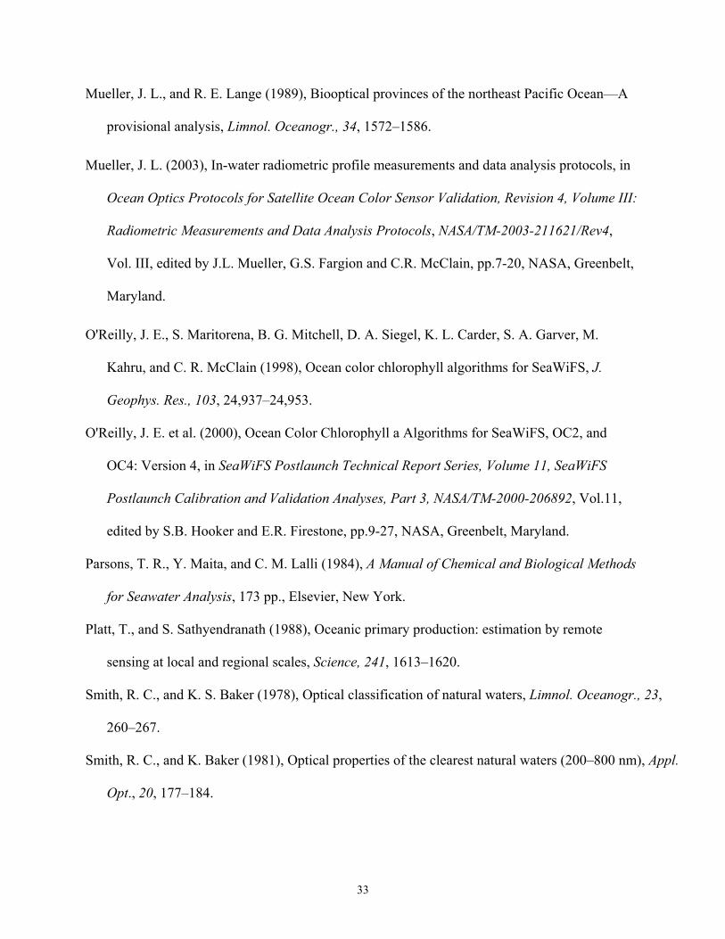
Mueller, J. L., and R. E. Lange (1989), Biooptical provinces of the northeast Pacific Ocean—A

provisional analysis, Limnol. Oceanogr., 34, 1572–1586.

Mueller, J. L. (2003), In-water radiometric profile measurements and data analysis protocols, in

Ocean Optics Protocols for Satellite Ocean Color Sensor Validation, Revision 4, Volume III:

Radiometric Measurements and Data Analysis Protocols, NASA/TM-2003-211621/Rev4,

Vol. III, edited by J.L. Mueller, G.S. Fargion and C.R. McClain, pp.7-20, NASA, Greenbelt,

Maryland.

O'Reilly, J. E., S. Maritorena, B. G. Mitchell, D. A. Siegel, K. L. Carder, S. A. Garver, M.

Kahru, and C. R. McClain (1998), Ocean color chlorophyll algorithms for SeaWiFS, J.

Geophys. Res., 103, 24,937–24,953.

O'Reilly, J. E. et al. (2000), Ocean Color Chlorophyll a Algorithms for SeaWiFS, OC2, and

OC4: Version 4, in SeaWiFS Postlaunch Technical Report Series, Volume 11, SeaWiFS

Postlaunch Calibration and Validation Analyses, Part 3, NASA/TM-2000-206892, Vol.11,

edited by S.B. Hooker and E.R. Firestone, pp.9-27, NASA, Greenbelt, Maryland.

Parsons, T. R., Y. Maita, and C. M. Lalli (1984), A Manual of Chemical and Biological Methods

for Seawater Analysis, 173 pp., Elsevier, New York.

Platt, T., and S. Sathyendranath (1988), Oceanic primary production: estimation by remote

sensing at local and regional scales, Science, 241, 1613–1620.

Smith, R. C., and K. S. Baker (1978), Optical classification of natural waters, Limnol. Oceanogr., 23,

260–267.

Smith, R. C., and K. Baker (1981), Optical properties of the clearest natural waters (200–800 nm), Appl.

Opt., 20, 177–184.

33

Stramska, M., D. Stramski, R. Hapter, S. Kaczmarek, and J. Ston (2003), Bio-optical

relationships and ocean color algorithms for the north polar regions of the Atlantic, J.

Geophys. Res., 108(C5), 3143, doi:10.1029/2001JC001195.

Stramski, D. (1999), Refractive index of planktonic cells as a measure of cellular carbon and

chlorophyll a content, Deep Sea Res., Part I, 46, 335–351.

Stramski, D., and A. Morel (1990), Optical properties of photosynthetic picoplankton in different

physiological states as affected by growth irradiance, Deep Sea Res., Part A, 37, 245–266.

Stramski, D., and R. A. Reynolds (1993), Diel variations in the optical properties of a marine

diatom, Limnol. Oceanogr., 38, 1347–1364.

Stramski, D., R. A. Reynolds, and B. G. Mitchell (1998), Relationships between the

backscattering coefficient and beam attenuation coefficient and particulate matter

concentrations in the Ross Sea, paper presented at Ocean Optics XIV Conference, ONR and

NASA Co-Sponsors, Kailua-Kona, Hawaii.

Stramski, D., R. A. Reynolds, M. Kahru, and B. G. Mitchell (1999), Estimation of particulate

organic carbon in the ocean from satellite remote sensing, Science, 285, 239–242.

Verity, P. G., C. Y. Robertson, C. R. Tronzo, M. G. Andrews, J. R. Nelson, and M. E. Sieracki

(1992), Relationships between cell volume and the carbon and nitrogen content of marine

photosynthetic nanoplankton, Limnol. Oceanogr., 37, 1434–1446.

Villafane, V., E. W. Helbling, and O. Holm-Hansen (1993), Phytoplankton around Elephant

Island, Antarctica, Polar Biol., 13, 183–191.

Volk, T., and M. I. Hoffert (1985), Ocean carbon pumps: Analysis of relative strengths and

efficiencies in ocean-driven atmospheric CO2 changes, in The Carbon Cycle and

34

Atmospheric CO2: Natural Variations Archean to Present, Geophys. Monogr. Ser., vol. 32,

edited by E. T. Sundquist and W. S. Broecker, pp. 99–110, AGU, Washington, D. C.

Woźniak, S. B., and D. Stramski (2004), Modeling the optical properties of mineral particles suspended

in seawater and their influence on ocean reflectance and chlorophyll estimation from remote sensing

algorithms, Appl. Opt., 43, 3489–3503.

Yoder, A. Y., C. R. McClain, G. C. Feldman, and W. E. Esaias (1993), Annual cycles of

phytoplankton chlorophyll concentrations in the global ocean: A satellite view, Global

Biogeochem. Cycles, 7, 181–193.

_________________

M. Stramska, Hancock Institute for Marine Studies, University of Southern California, Los

Angeles, CA 90089-0371, USA. (stramska@usc.edu)

D. Stramski, Marine Physical Laboratory, Scripps Institution of Oceanography, University of

California at san Diego, La Jolla, CA 92093-0238, USA. (dstramski@ucsd.edu)

35

Figure 1. Locations of stations during the cruise of R/V Polarstern in 2003 in the north polar

Atlantic where water sampling and underwater optical measurements were made.

Figure 2. Example vertical profiles of the particulate beam attenuation coefficient, cp(660) (solid

and dashed lines), and the corresponding particulate organic carbon (POC) estimates from

analysis of water samples taken at discrete depths (solid and open circles). The data were

collected on R/V Polarstern at station 18 (3 May 2003; 0830 GMT; 75.0ºN, 4.12ºW), station 20

(4 May 2003; 1000 GMT; 75.0ºN, 6.07ºW), station 22 (5 May 2003; 0930 GMT; 75.0ºN,

9.93ºW), and station 25 (6 May 2003; 1000 GMT; 75.0ºN, 12.63ºW).

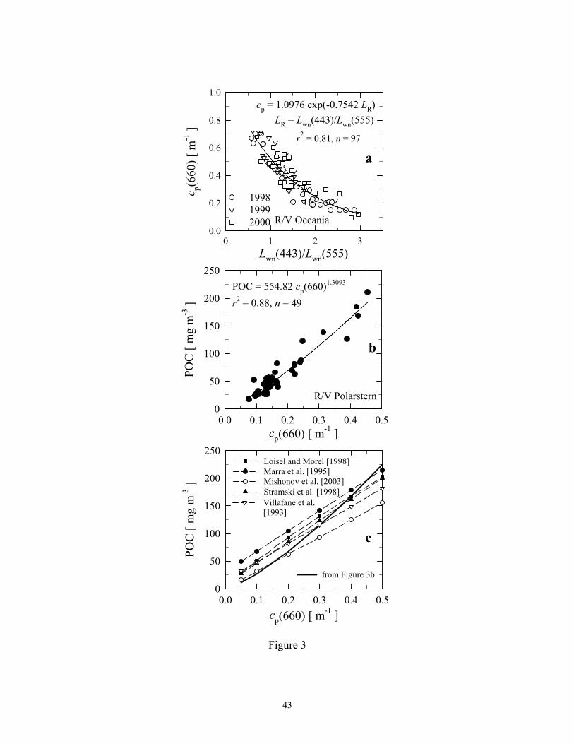
Figure 3. (a) Beam attenuation coefficient of particles at 660 nm, cp(660), versus the spectral

ratio of normalized water-leaving radiance, Lwn(443)/Lwn(555). Data collected in the north polar

Atlantic in 1998, 1999, and 2000 are indicated by circles, triangles, and squares, respectively.

The solid line is the best exponential fit to the data. The best fit equation, the squared correlation

coefficient r2, and the number of observations n are also shown. (b) Particulate organic carbon

concentration in surface waters as a function of the beam attenuation coefficient, cp(660). Data

were collected in the north polar Atlantic in 2003. The solid line is the best power function fit to

the data. The corresponding equation and the values of r2 and n are also shown. (c) Comparison

of the POC versus cp(660) relationship for our study region (solid line) with similar relationships

established by various investigators in other regions (dashed lines). The Loisel and Morel [1998]

line represents their regression on the basis of data from the upper homogeneous layer in the

north Atlantic and Pacific near Hawaii; the Villafane et al. [1993] line represents an average

36

from their two cruises in the Southern Ocean near Elephant Island; the Marra et al. [1995] line is

from the northeast Atlantic; the Mishonov et al. [2003] line is from the north Atlantic; and the

Stramski et al. [1998] line is from the Ross Sea.

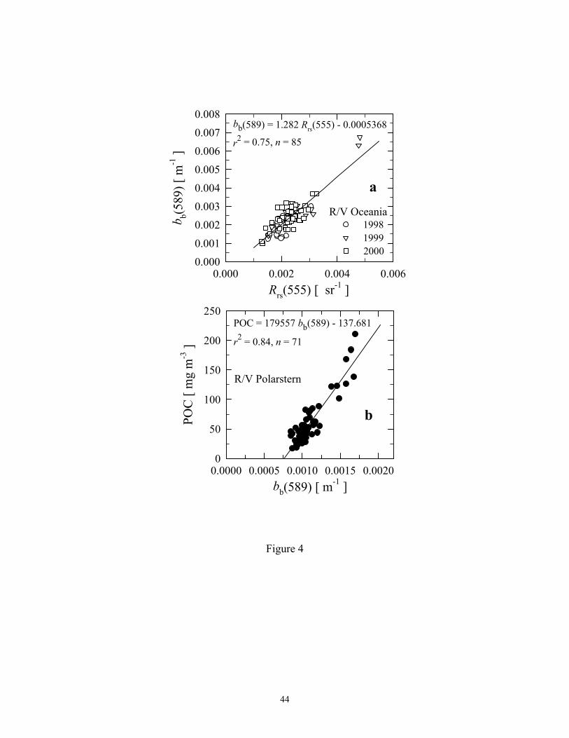
Figure 4. (a) Backscattering coefficient of seawater at 589 nm, bb(589), as a function of remote-

sensing reflectance at 555 nm, Rrs(555). Data collected in the north polar Atlantic in 1998, 1999,

and 2000 are indicated by circles, triangles, and squares, respectively. (b) Particulate organic

carbon concentration in surface waters as a function of backscattering coefficient, bb(589). Data

were collected in the north polar Atlantic in 2003. Solid lines represent the best linear fit to the

data. The corresponding equations and the values of r2 and n are also shown.

Figure 5. Concentration of particulate organic carbon as a function of chlorophyll a

concentration. Data were collected in the north polar Atlantic in 2003. The solid line is the best

linear fit to the data. The corresponding equation and the values of r2 and n are also shown.

Figure 6. (a) Particulate organic carbon concentration versus the spectral ratio of remote-sensing

reflectances, Rrs(490)/Rrs(555). Data were obtained from the public databases of the U. S. Joint

Global Ocean Flux Study (U.S. JGOFS) and the NASA Sensor Intercomparison for Marine

Biological and Interdisciplinary Ocean Studies (SIMBIOS) programs. (b) As in Figure 6a but for

the reflectance ratio Rrs(443)/Rrs(555). Solid lines represent the best power function fit to the

data. The corresponding equations and the values of r2 and n are also shown.

37

Figure 7. Comparison of particulate organic carbon estimates obtained from the five algorithms.

The input to the algorithms was the SeaWiFS monthly composite data for May 2003 at transects

along 79ºN, 75ºN, and 71ºN. POC estimates 1–4 are based on the algorithms presented in

Figures 3–6. POC estimate 5 is based on the algorithm proposed by Mishonov et al. [2003].

Figure 8. (a) POC estimate 4 (open circles) and (b) POC estimates 2 (solid triangles) and 3 (open

triangles) plotted versus POC estimate 1. All these estimates were derived from SeaWiFS

monthly composites for the month of May from the 6-year period (1998–2003) along 71ºN in the

north polar Atlantic.

Figure 9. (a) Comparison of in situ POC and satellite-derived POC from algorithms 1 and 4.

Data represent match-ups for the field measurements taken on the R/V Oceania cruises in 1998

and 1999 and the satellite measurements (HRPT data) from concurrent SeaWiFS overpasses in

the north polar Atlantic. POC estimates derived from algorithms 1 and 4 are indicated by solid

circles and open circles, respectively. (b) Comparison of in situ POC and satellite-derived POC

from algorithm 4. Data represent match-ups for the concurrent satellite and field measurements

taken during several research projects in various oceanic regions as indicated.

Figure 10. Spatial and interannual variability of surface POC in the month of April in the north

polar Atlantic as derived from SeaWiFS data using algorithm 1 shown in Figure 3. The data

shown as open circles, triangles, and squares indicate monthly POC values. Solid circles indicate

monthly POC averaged over the 6-year period (1998–2003). All data points represent POC

38

averaged over the grid size of 1º by 1º. For example, the data point at 1ºE and 75ºN represents

the POC averaged over the area delimited by 74.5ºN, 75.5ºN, 0.5ºE, and 1.5ºE.

Figure 11. As in Figure 10 but for May.

Figure 12. As in Figure 10 but for June.

Figure 13. As in Figure 10 but for July.

Figure 14. As in Figure 10 but for August.

Figure 15. Interannual and spatial variability of seasonally (April through August) averaged

surface POC as derived from 6 years (1998–2003) of the SeaWiFS data using our algorithm 1.

(a) Data for the latitudes between 70ºN and 74ºN. (b) Data for the latitudes between 75ºN and

79ºN. In each graph, we show the seasonally averaged POC for each year (open circles, triangles,

and squares) and the 6-year average seasonal POC (solid circles).

Figure 16. (a) Regionally averaged monthly POC concentrations for different years plotted as a

function of month, where 4 is April, 5 is May, 6 is June, 7 is July, and 8 is August. (b)

Regionally averaged seasonal POC concentrations as a function of year.

39

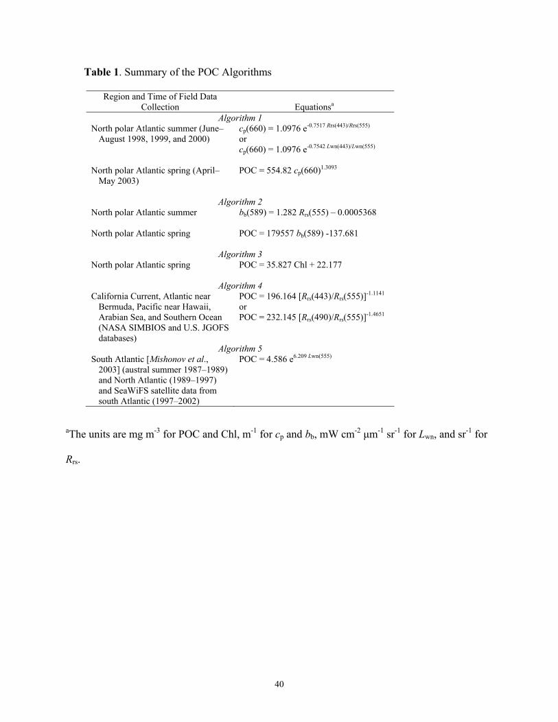
Table 1. Summary of the POC Algorithms

Region and Time of Field Data Collection Equationsa

Algorithm 1 North polar Atlantic summer (June–

August 1998, 1999, and 2000) cp(660) = 1.0976 e-0.7517 Rrs(443)/Rrs(555) or cp(660) = 1.0976 e-0.7542 Lwn(443)/Lwn(555)

North polar Atlantic spring (April–May 2003)

POC = 554.82 cp(660)1.3093

Algorithm 2 North polar Atlantic summer

bb(589) = 1.282 Rrs(555) – 0.0005368

North polar Atlantic spring

POC = 179557 bb(589) -137.681

Algorithm 3 North polar Atlantic spring

POC = 35.827 Chl + 22.177

Algorithm 4 California Current, Atlantic near

Bermuda, Pacific near Hawaii, Arabian Sea, and Southern Ocean (NASA SIMBIOS and U.S. JGOFS databases)

POC = 196.164 [Rrs(443)/Rrs(555)]-1.1141 or POC = 232.145 [Rrs(490)/Rrs(555)]-1.4651

Algorithm 5 South Atlantic [Mishonov et al.,

2003] (austral summer 1987–1989) and North Atlantic (1989–1997) and SeaWiFS satellite data from south Atlantic (1997–2002)

POC = 4.586 e6.209 Lwn(555)

aThe units are mg m-3 for POC and Chl, m-1 for cp and bb, mW cm-2 µm-1 sr-1 for Lwn, and sr-1 for

Rrs.

40

Figure 1

41

cp(660) [ m-1 ]0.1 0.2 0.3 0.4 0.5

dept

h [ m

]

100

80

60

40

20

0

POC [ mg m-3 ]0 50 100 150 200

cp(660) [ m-1 ]0.1 0.2 0.3 0.4 0.5

100

80

60

40

20

0

POC [ mg m-3 ]0 50 100 150 200

station 18station 25

station 20 station 22

Figure 2

42

Lwn(443)/Lwn(555)0 1 2 3

c p(66

0) [

m-1

]

0.0

0.2

0.4

0.6

0.8

1.0

cp(660) [ m-1 ]0.0 0.1 0.2 0.3 0.4 0.5

POC

[ m

g m

-3 ]

0

50

100

150

200

250

R/V Oceania

R/V Polarstern

POC = 554.82 cp(660)1.3093

r2 = 0.88, n = 49

1998 19992000

a

b

cp(660) [ m-1 ]0.0 0.1 0.2 0.3 0.4 0.5

POC

[ m

g m

-3 ]

0

50

100

150

200

250

c

from Figure 3b

Mishonov et al. [2003]Stramski et al. [1998]Villafane et al.[1993]

Marra et al. [1995]Loisel and Morel [1998]

cp = 1.0976 exp(-0.7542 LR) LR = Lwn(443)/Lwn(555)

r2 = 0.81, n = 97

Figure 3

43

Rrs(555) [ sr-1 ]0.000 0.002 0.004 0.006

b b(589

) [ m

-1 ]

0.000

0.001

0.002

0.003

0.004

0.005

0.006

0.007

0.008

bb(589) [ m-1 ]0.0000 0.0005 0.0010 0.0015 0.0020

POC

[ m

g m

-3 ]

0

50

100

150

200

250POC = 179557 bb(589) - 137.681

r2 = 0.84, n = 71

R/V Polarstern

199819992000

R/V Oceania

bb(589) = 1.282 Rrs(555) - 0.0005368

r2 = 0.75, n = 85

a

b

Figure 4

44

Chl [ mg m-3 ]0 1 2 3 4 5 6

POC

[ m

g m

-3 ]

0

50

100

150

200

250

R/V Polarstern

POC = 35.827 Chl + 22.177r2 = 0.94, n = 77

Figure 5

45

Rrs(490)/Rrs(555)0 1 2 3 4 5

POC

[ m

g m

-3 ]

10

100

1000 POC = 232.145 X -1.4651

X = Rrs(490)/Rrs(555) r2 = 0.82, n = 205

Rrs(443)/Rrs(555)0 1 2 3 4 5 6 7

POC

[ m

g m

-3 ]

10

100

1000 POC = 196.164 X -1.1141

X = Rrs(443)/Rrs(555) r2 = 0.80, n = 205

CalCOFI (1998) BATS (1998)HOTS (1998)JGOFS Arabian Sea (1995)JGOFS Southern Ocean (1997-98)

a

b

Figure 6

46

-10 -5 0 5 10

POC

[ m

g m

-3 ]

10

100

-10 -5 0 5 10

POC

[ m

g m

-3 ]

10

100

Longitude [degrees]

-10 -5 0 5 10

POC

[ m

g m

-3 ]

10

100

71 oN

75 oN

79 oN

May 2003

algorithm 3

algorithm 1algorithm 2

algorithm 5algorithm 4

Figure 7

47

May 1998-2003 at 71oN

Y = X

POC estimate 10 100 200 300 400 500

POC

est

imat

e 4

[ mg

m-3

]

0

100

200

300

400

500

POC estimate 1 [ mg m-3 ]0 100 200 300 400 500PO

C e

stim

ates

2 a

nd 3

[ m

g m

-3 ]

0

100

200

300

400

500

1:1 line

estimate 2

1:1 lineestimate 3

a

b

Figure 8

48

in situ POC [mg m-3 ]0 50 100 150 200 250 300

sate

llite

-der

ived

PO

C [

mg

m-3

]

0

50

100

150

200

250

300

algorithm 1algorithm 4

in situ POC [ mg m-3 ]0 50 100 150 200 250 300

sate

llite

-der

ived

PO

C [

mg

m-3

]

0

50

100

150

200

250

300

HOTS (1998-99)BATS (1998)

CalCOFI (1998)

JGOFS Southern Ocean (1998)CARIACO (1998)

a

b

1:1 line

1:1 line

Legend for panel b

north polar Atlantic

Figure 9

49

Longitude [ degrees ]-10 -5 0 5 10

POC

[ m

g m

-3]

10

100

1998 1999 2000

-10 -5 0 5 10

POC

[ m

g m

-3 ]

10

100

-10 -5 0 5 10

POC

[ m

g m

-3 ]

10

100

6-year average

April

79oN

75oN

71oN

2001 2002 2003

Figure 10

50

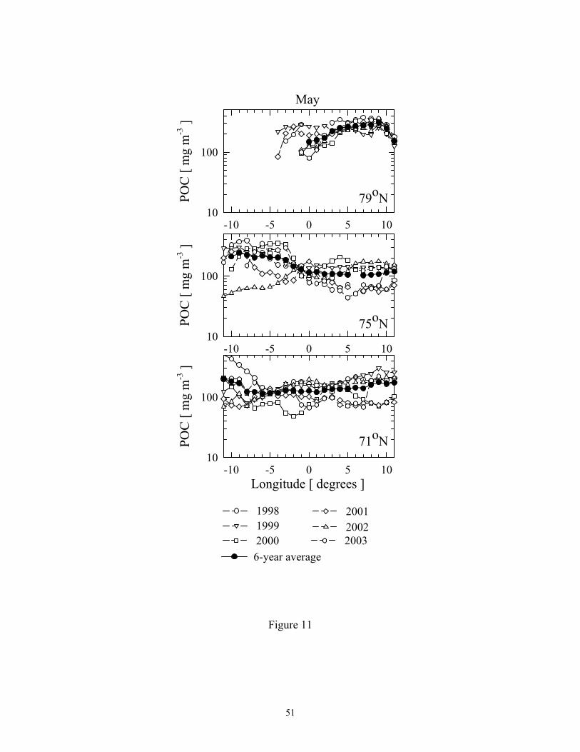
Longitude [ degrees ]-10 -5 0 5 10

POC

[ m

g m

-3 ]

10

100

-10 -5 0 5 10

POC

[ m

g m

-3 ]

10

100

-10 -5 0 5 10

POC

[ m

g m

-3 ]

10

100

6-year average

May

79oN

75oN

71oN

1998 1999 2000

2001 2002 2003

Figure 11

51

Longitude [ degrees ]-10 -5 0 5 10

POC

[ m

g m

-3 ]

10

100

-10 -5 0 5 10

POC

[ m

g m

-3 ]

10

100

-10 -5 0 5 10

POC

[ m

g m

-3 ]

10

100

6-year average

June

79oN

75oN

71oN

1998 1999 2000

2001 2002 2003

Figure 12

52

Longitude [ degrees ]-10 -5 0 5 10

POC

[ m

g m

-3 ]

10

100

-10 -5 0 5 10

POC

[ m

g m

-3 ]

10

100

-10 -5 0 5 10

POC

[ m

g m

-3 ]

10

100

6-year average

July

79oN

75oN

71oN

2001 2002 2003

1998 1999 2000

Figure 13

53

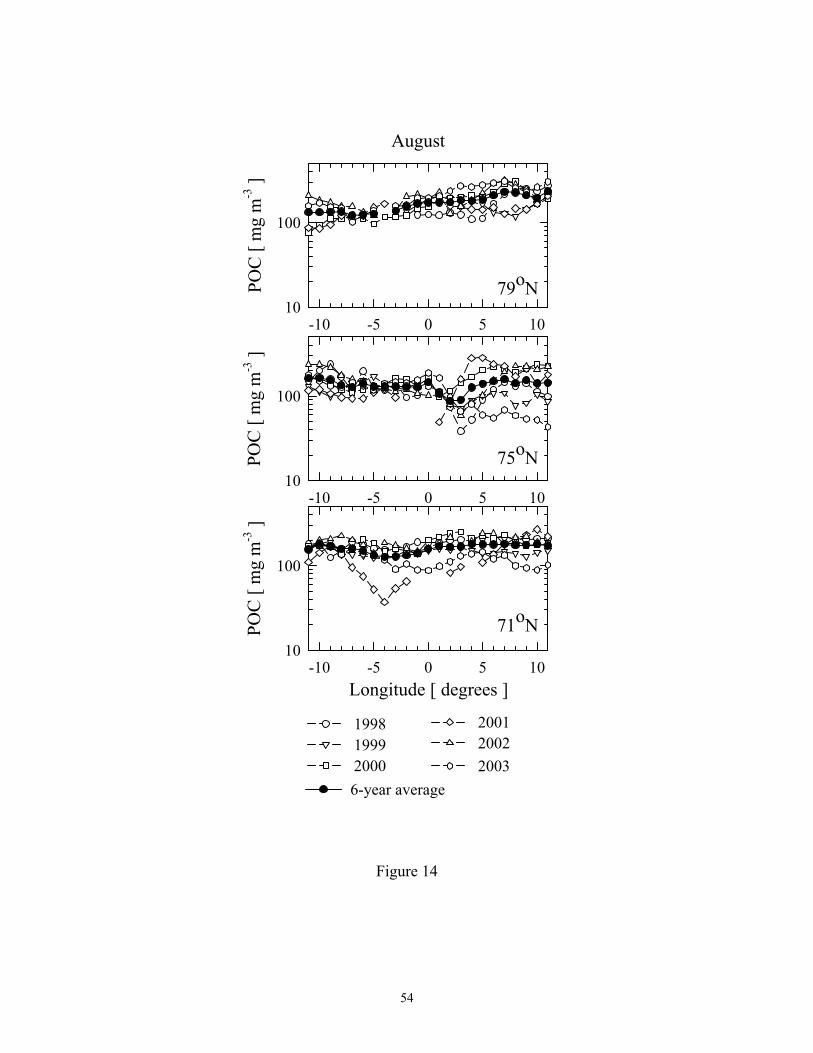
Longitude [ degrees ]-10 -5 0 5 10

POC

[ m

g m

-3 ]

10

100

-10 -5 0 5 10

POC

[ m

g m

-3 ]

10

100

-10 -5 0 5 10

POC

[ m

g m

-3 ]

10

100

August

79oN

75oN

71oN

6-year average

2001 2002 2003

1998 1999 2000

Figure 14

54

Longitude [degrees ]-10 -5 0 5 10

50100150200250300

50100150200250300

POC

[ m

g m

-3]

50100150200250300

50100150200250300

50100150200250300

75 oN

76 oN

77 oN

78 oN

79 oN

Longitude [ degrees ]-10 -5 0 5 10

50100150200250300

50100150200250300PO

C [

mg

m-3

]

50100150200250300

50100150200250300

50100150200250300

70 oN

71 oN

72 oN

73 oN

74 oN

6-year average seasonal POC

1998 1999 2000

2001 2002 2003

a b

Figure 15

55

Month4 5 6 7 8

POC

[ m

g m

-3 ]

0

50

100

150

200

250

Year1998 1999 2000 2001 2002 2003

POC

[ m

g m

-3 ]

130135140145150155160165170

1998 1999 2000

2001 2002 2003

a

b

Figure 16

56