variability and singularity arising from poor compliance
TRANSCRIPT

HAL Id: hal-00868621https://hal.inria.fr/hal-00868621
Submitted on 1 Oct 2013
HAL is a multi-disciplinary open accessarchive for the deposit and dissemination of sci-entific research documents, whether they are pub-lished or not. The documents may come fromteaching and research institutions in France orabroad, or from public or private research centers.
L’archive ouverte pluridisciplinaire HAL, estdestinée au dépôt et à la diffusion de documentsscientifiques de niveau recherche, publiés ou non,émanant des établissements d’enseignement et derecherche français ou étrangers, des laboratoirespublics ou privés.
Variability and singularity arising from poor compliancein a pharmacokinetic model II: the multi-oral case
Lisandro J. Fermin, Jacques Lévy Véhel
To cite this version:Lisandro J. Fermin, Jacques Lévy Véhel. Variability and singularity arising from poor compliance ina pharmacokinetic model II: the multi-oral case. Journal of Mathematical Biology, Springer Verlag(Germany), 2016, �10.1007/s00285-016-1041-1�. �hal-00868621�

Variability and singularity arising from poorcompliance in a pharmacokinetic model
II: the multi-oral case
L.J. Fermın 1,2 and J. Levy Vehel 2
1 CIMFAV, Faculty of Engineering, University of Valparaiso, Valparaiso, Chile.2 Regularity Team, INRIA Saclay-Ile-de-France & MAS Laboratory, Ecole Centrale Paris, France.
Abstract
We study a simplified model for the drug concentration in the case of multiple oraldoses and in a situation of poor patient compliance. Our model is a stochastic one, whichis able to take into account an irregular drug intake schedule. This article is the second in aseries of three. It presents a multi-oral version of the results given in [11], that dealt with themulti IV case. Under some assumptions, we study features of the drug concentration thathave practical implications, such as its variability and the regularity of its probability dis-tribution. We consider four variants: continuous-time, with either deterministic or randomdoses, and discrete-time, also with either deterministic or random doses. Our computationsallow one to assess in a precise way the effect of various significant parameters such asthe mean rate of intake, the elimination rate, the absorption rate and the mean dose. Theyquantify how much poor compliance will affect the regimen. To appreciate this impact,we provide detailed comparisons with the variability of concentration in the cases of botha fully compliant patient and a population of fully compliant patients with log-normalydistributed pharmacokinetic parameters. Besides, the discrete-time versions of our mod-els reveal unexpected links with possibly multifractal measures known in mathematics asinfinite Bernoulli convolutions. Analogously to the multi-IV case, we find that the distri-bution of the concentration in this model is either absolutely continuous or purely singular,depending on a relevant parameter. Our results complement the ones in [11] and help un-derstanding the consequences of poor compliance. They may have practical outcomes interms of drug dosing and scheduling.

Contents1 Introduction 3
2 Overview: pharmacokinetic implication of non compliance 42.1 Purely deterministic model (full compliance) . . . . . . . . . . . . . . . . 42.2 Full compliance with population parameter variability . . . . . . . . . . . . 72.3 Continuous model with random intake instants and deterministic doses . . . 102.4 Continuous model with random intake instants and random doses . . . . . . 162.5 Discrete model with random intake instants and deterministic doses . . . . 182.6 Discrete model with random intake instants and random doses . . . . . . . 19
3 Continuous model with random intake instants and deterministic doses 203.1 Variability of the concentration . . . . . . . . . . . . . . . . . . . . . . . . 213.2 Regularity of the limit distribution . . . . . . . . . . . . . . . . . . . . . . 22
4 Continuous model with random intake instants and random doses 254.1 Variability of the concentration . . . . . . . . . . . . . . . . . . . . . . . . 254.2 Regularity of the limit distribution . . . . . . . . . . . . . . . . . . . . . . 28
5 Discrete model with random intake instants and deterministic doses 295.1 The discretized concentration . . . . . . . . . . . . . . . . . . . . . . . . . 295.2 Variability of the discretized concentration . . . . . . . . . . . . . . . . . . 315.3 Limit when the discretization step tends to 0 . . . . . . . . . . . . . . . . . 325.4 Regularity of the discretized model . . . . . . . . . . . . . . . . . . . . . . 32
6 Discrete model with random intake instants and random doses 336.1 Variability of the concentration . . . . . . . . . . . . . . . . . . . . . . . . 346.2 Limit when the discretization step tends to 0 . . . . . . . . . . . . . . . . . 34
2

1 IntroductionIn the seminal work [13], the authors attacked the problem of mathematically modelingpoor compliance using a probabilistic frame. They considered general distributions forthe random instants of drug intake and studied the mean and variance of the concentrationconditioned on the time elapsed since the last intake. Various related models were studied indetail in [11]: the probability distribution of drug concentration in the context of multiple-IV dosing and poor compliance was investigated when both the times of intakes and dosesare supposed to be random. In addition, both continuous-time and discrete-time versionswere considered.
The present work parallels the studies of [11] in the more realistic framework of mul-tiple oral dosing. As in [11], we investigate below the probability distribution of drugconcentration in the context of poor compliance: the instants of drug intake are randoms,with possibly random doses. We use the simplest possible law to model the random timesof drug intake, i.e. a homogeneous Poisson distribution. In other words, the times of drugintake are supposed to follows a Poisson process. This assumption allows one to performexplicit computations using the well-developed machinery on Poisson processes, and toobtain precise results describing various aspects of the distribution of the concentrationthat are important for assessing the efficacy of the regimen. We focus on two aspects ofpractical relevance: the variability of the concentration and the regularity of its probabilitydistribution.
Our results quantify the variability of the concentration around its mean showing theexact role played by each parameter of the process. We measure how much poor compli-ance increases this variability as compared to the full compliance case. We show that theprobability distribution limit of drug concentration may display irregular behaviours: inour case this occurs when the ratio between the mean number of intakes per unit time andthe minimum between the elimination rate and the absorption rate is smaller than one half.When the same ratio is smaller than one, it becomes singular (i.e. non differentiable) atthe origin. In practical terms, this amounts to quantifying, in a precise way, the situationswhere the moments of intakes are too scarce (with respect to the elimination and absorptionrates), resulting in a high probability of having too small a concentration of drugs.
We also study a discrete-time version of the model. This setting reveals unexpectedlinks with multifractal measures which have been studied in the mathematical literature forover seventy years under the name of infinite Bernoulli convolutions. Again, dependingon some parameters, the discretized concentration may exhibit an extremely irregular be-haviour. This means that the probability of observing a concentration C depends in a verynon-smooth way on the precise value of C. This is obviously an undesirable feature whichmay have strongly negative consequences.
As mentioned above, the present article is the second in a series of three, where thefirst work [11] dealt with the multi IV case. Since some computations here are very similarto this case, they are omitted and the interested reader is referred to [11] for full details.The third paper in the series, [4], extends our results by considering more realistic random
3
schedules for the time instants of drug intakes: indeed, the use a homogeneous Poissonlaw is mathematically handy, but somewhat restrictive: in real situations, the schedule isprobably much more complex. [4] uses the powerful mathematical framework known asPiecewise Deterministic Markov Model to deal with general drug intake schedules, at theexpense of a more complex theoretical apparatus.
We do not address in this work the problem of estimating the parameters of the variousmodels, in particular the law of the random intake times and doses. A recent article dealingwith this issue is [2].
The remaining of this work is organized as follows: for the reader’s convenience, wepresent an overview of our main findings pertaining to the various models and their practicalimplications in Section 2. In particular, we compare the variabilities in our poor compliancemodels to the ones in the cases of (a) full compliance of a single patient and (b) full com-pliance in a population where one takes into account variability due to differing eliminationrates or clearances between individuals. This allows us to highlight “equivalent scenarios”where, for instance, we find the parameters of a non-compliant patient that will yield thesame variance in concentration as in a whole population with given distribution of elimina-tion rates, or, which is the same, of a single individual whose elimination rate is unknownand is modelled as a random variable. A reader not interested in the mathematical detailsmay concentrate on Section 2 to get a quick summary of our work, and refer if needed to thedetails in the following sections. In Section 3, we set up the basic continuous time modelfor deterministic dose random time drug intake and study its variability (Section 3.1) andregularity (Section 3.2). In Section 4, we analyse the random doses version of this model.As before, we study its variability (Section 4.1) and regularity (Section 4.2). We present thediscrete-time version of the deterministic dose random time model in Section 5. We derivethe discrete time concentration in Section 5.1 and study its variability in Section 5.2. In Sec-tion 5.3, we show that the discrete-time model tends to the continuous-time one when thediscretization step tends to 0. Section 5.4 describes the complex regularity behaviour of theprobability distribution of the concentration in the discrete-time model. Finally, Section 6deals with the discrete-time random-dose case: its variability is described in Section 6.1,and its limiting behaviour when the discretization step tends to 0 is studied in Section 6.2.
2 Overview: pharmacokinetic implication of non com-pliance
2.1 Purely deterministic model (full compliance)To assess the impact of poor compliance, it is useful to contrast it with situations of fullcompliance. We derive in this section the variability in concentration for a single fullycompliant patient. The next section will deal with the variability in a population of fullycompliant patients.
4

Let us first recall the basic equations. We consider in this work the case of multiplesoral administration and we suppose that kinetics of first order are involved. Our first modelis a very classical one: it assumes that the patient takes orally a constant dose D at regularlyspaced times t0, t1, . . . , tn, . . ., with ti =
iλ , that is, the patient takes drugs every 1
λ units oftimes for some positive λ.
For completeness and future use, we briefly recall how the equations governing the ab-sorption and elimination processes are obtained. The oral absorption process is concernedwith the amount of drug at the absorption site remaining to be absorbed. The amount ofdrug at the absorption site, denoted Aoral, is characterized by the absorption coefficient rateka. At each drug intake time ti, Aoral(t) increases by D. Between ti and ti+1, the effect ofthe dose taken at ti decreases exponentially fast, with exponential speed ka. Formally:
d
dtAoral(t) =
∑i:ti≤t
Dδ(t− ti)− kaAoral(t), (1)
with δ denoting the Dirac distribution. Thus, the rate of absorption of drug at time t iskaFAoral(t), where F is the absolute bioavailability; i.e. the fraction of each dose whichis absorbed when the drug is given by the oral route.
The elimination process describes by the irreversible loss of drug from the site of mea-surement. We assume that the drug is eliminated with a constant elimination rate ke. De-noting Acentral the amount of drug in the body, one gets that the rate of elimination of drugis keAcentral.
The model is given from mass balance considerations: at any given time, the dose isaccounted for by the amount of drug at absorption site plus the amount of drug in body plusthe amount of eliminated drug. Thus, the sum of the rates of change of the drug in thesecompartments must equal zero, so that the rate of change of drug in body is equal to therate of absorption minus the rate of elimination. This leads to:
d
dtAcentral(t) = kaFAoral(t)− keAcentral(t). (2)
The drug concentration at time t is defined by
C(t) =Acentral(t)
Vd, (3)
where Vd is the apparent volume of distribution of the drug with respect to its concentrationin plasma.
The solution of equation (1) is
Aoral(t) = D∑i
e−ka(t−ti)1l(t≥ti), (4)
where 1l(t≥ti) denotes the indicator function of the set {t ∈ R : t ≥ ti)}, which equals 1 ift ≥ ti and 0 otherwise.
5

Applying the parameter-variation method to equation (2) one obtains, from equations(3) and (4), the following expression for the deterministic drug concentration process Cd:
Cd(t) =FD
Vd
kaka − ke
∑i
(e−ke(t−ti) − e−ka(t−ti)
)1l(t≥ti). (5)
We will wish to compare the values of the expectation and the variance in variousstochastic models to the one in the case of full compliance. Of course, in the frame offull compliance, there is no randomness involved, and one cannot define proper mean andvariance. However, since the concentration varies in time, it makes sense to define the meanas the average of concentration over all values of t, and to define the variance correspond-ingly. In other words, we denote:
Ed = limT→∞
1
T
∫ T
0Cd(t)dt, (6)
V ard = limT→∞
1
T
∫ T
0(Cd(t)− Ed)
2 dt (7)
for the mean and variance with respect to time of Cd(t). Note that Ed is closely relatedto the usual PK metric AUC. V ard represent the time-average square deviation from thelong term average Ed. Simple computations lead to:
Ed = µeFD
Vd, (8)
V ard =µe
2
(FD
Vd
)2 [ 1
1 + r+G(r)
]. (9)
where
G(r) =2
1− r2
(1
e1/µe − 1− r
e1/rµe − 1
)− 2µe, (10)
µe := λke
, µa := λka
and r := keka
= µa
µe. These quantities are related to ones considered in
[14].For comparison with the random models below, we note the following facts:
• When µa → 0, we are in the case of instantaneous absorption, which is equivalent tothe multi-IV case. In this frame, we recover the results of [11].
• In Formula (9), the term G(r), given by Formula (10), is always negative, as mayeasily be checked.
• The term G(r), seen as a function of r, is increasing. It is thus minimum when requals 0, and it tends to 0 when r tends to infinity.
• When µe tends to 0, the variance tends to 0 at rate µ2e when µa = 0 and at rate µe
when µa = 0.
6

• For a fixed mean Ed = 1, and when µe tends to infinity, V ard tends to 0 at speed 1µ2e.
When µe tend to 0, the variance tends to 12µa
when µa = 0, and to infinity at speed1µe
when µa = 0.
• P(|Cd − E(Cd)| ≥ γE(Cd)) ≤ 1µ∗2γ2 for γ large enough, where µ∗ = max{µe, µa}
(see Formula (25) for a more precise expression). Assume µa, µe tend to infinity atthe same rate. Then, the bound is 1
µ∗4γ2 .
These formulas quantify the obvious fact that the variability of concentration is a de-creasing function of the number of takes per unit time. As we show below, non complianceamplifies the variability of the concentration in a way we will precisely measure.
2.2 Full compliance with population parameter variabilityIn the previous section, we have characterized the variability for a deterministic PK modeldefined by a unique set of PK parameters, i.e. the case of a single compliant subject withperfectly known pharmacokinetic parameters. We now investigate variability in a Pop-PKmodel for the case of a whole population. A Pop-PK involve randomly distributed PKparameter to reflect the peculiarity of each patient and other unexplained variability. Atypical assumption is to consider that individual parameters are log-normally distributed inthe population. The log-normal distribution is a common modelling for positive continuousquantities, and seems to fit well with the finding of large scale Pop-PK studies [8, 18]. Wealso assume that each subject in the population is fully compliant and that their drug intakefrequency λ is the same.
Let us first consider the case where the elimination rate is random and the other param-eters such as D, Vd, F , ka are constants. This amounts to replacing ke by keUke in thepreceding computations, where ke is the typical parameter value of the population and Uke
is a dimensionless random variable that represent the variability among subject, which isassumed to follows a log-normal distribution with parameters mke = 0 and σ2
ke. The choice
mke = 0 ensures that the reference value ke is the median of the distribution. We wish toexamine the impact of this variability on the long-term average concentration Ed, given byequations (6) and (8). The variability of Ed is solely due to the variation of keUke . In otherwords, we consider the variable Ed(keUKe) with Uke following a log-normal distribution,and measure its variability. Thus, the mean and variance of Ed across the population aregiven by:
Epop(Ed) =λ
ke
FD
VdEpop
(1
Uke
)=
λ
ke
FD
Vdeσ
2ke
/2,
Varpop(Ed) =
(λ
ke
FD
Vd
)2
Varpop
(1
Uke
)=
(λ
ke
FD
Vd
)2
eσ2ke
(eσ
2ke − 1
).
Let us rewrite these formulas in terms µe and the coefficient of variation of the elimi-
7

nation rate CVke =
√eσ
2ke − 1:
Epop(Ed) = µeFD
Vd
√1 + CV 2
ke,
Varpop(Ed) =
(µe
FD
Vd
)2
CV 2ke
(1 + CV 2
ke
).
The same approach applies if one wishes to take into account in addition the variabilityof Vd and F across the population. In this case, ka is assumed constant and one simulta-neously replaces ke by keUke , Vd by VdUVd
and F by FUF , where Uke , UVdand UF are
random variables log-normally distributed with median parameters mke = 0, mVd= 0,
mF = 0 and variability parameters σ2ke
, σ2Vd
, σ2F respectively. To perform the computa-
tions, the knowledge of the joint distribution of Uke and UVd, or at least that of UkeUVd
isneeded. Joint distributions are not usually reported in Pop-PK studies, but since the productkeVd is nothing but the clearance Cl, we can see that in this case we have:
Cl = keUkeVdUVd= Cl0UCl,
where Cl0 = keVd and UCl = UkeUVdrepresent the variability of clearance, whose dis-
tribution is more frequently reported in Pop-PK studies. Note that the log-normality ofclearance typically reported in the literature is compatible with the joint log-normality of(Uke , UVd
). Thus, if we assume that UCl and UF are log-normally distributed randomvariables with parameters mCl = 0, mF = 0 and variability parameters σ2
Cl, σ2F re-
spectively, and we assume that the variables UCl and UF are correlated with correlationρ = cov(log(Uke), log(UVd
))/σClσF ∈ [−1, 1], computations similar to the ones abovelead to:
Epop(Ed) = µeFD
Vd
√1 + CV 2, (11)
Varpop(Ed) =
(µe
FD
Vd
)2
CV 2(1 + CV 2
), (12)
where CV =√
eσ2Cl+σ2
F+2ρσClσF − 1 is the coefficient of total variation. Note that indi-vidual variations of F are difficult to distinguish from ones of Cl. We have therefore chosento control the variability through the coefficient of total variation CV , which encompassesthe variability of ke, Vd and F .
For consistency, we will always use in the sequel the following PK parameters similarto those of imatinib, see [2, 3, 19]. They are given in Table 1.
8

Parameter Unit TV SD CV (%)
D mg 150 0 0%ka h−1 0.61 0 0%F 1 0.2462 25%Cl lh−1 14.3 0.3491 36%Vd l 347 0.5781 63%
Table 1: PK parameters of imatinib. TV: Typical Value; SD: Standard Deviation; CV: Coefficient of variation.
Suppose that the correlation parameter ρ is 0. Then the coefficient of total variation isCV = 44.74%, which correspond to a standard deviation of 0.4272. Assuming that dosesare taken every 1
λ = 12h, one obtains for the mean and variance:
Epop(Ed) = 0.9576mg/l, and Varpop(Ed) = 0.1836mg2/l2,
where we have assumed for simplicity that Vd is constant, i.e. Cl = keVdUke , where Uke islog-normal with parameters mke = 0 and σ2
ke= σ2
Cl.Note that the coefficient of total variation CV is an increasing function of ρ, that reaches
its maximum CVmax = 65.22% when ρ = 1 and its minimum CVmin = 10.31% whenρ = −1.
0 50 100 150 200 250 3000
0.2
0.4
0.6
0.8
1
1.2
1.4
1.6
1.8
2
time (h)
Con
cent
ratio
n (m
g/l)
Figure 1: Eight sample paths of the concentration taking into account variability of clearance and bioavailability,graphed for the first fourteen days. The black solid line is the population mean µpop, the dotted-dashed linescorrespond to the confidence bands µpop ± σpop and the dashed lines to the confidence bands µpop ± 2σpop.
We display on Figure 1 eight sample evolutions of the concentration for the first 14 daysin this scenario. The simulations show that a steady state is quickly reached. In addition, all
9

but one samples lie within one standard deviation σpop =√
Varpop(Ed) of the populationmean µpop = Epop(Ed).
In the following sections, we return to the case of a single subject with perfectly knownPK parameters, but with poorly compliant behaviour, and we will compare the variabilityin the various cases.
2.3 Continuous model with random intake instants and deter-ministic dosesIn the context of poor compliance the ti are not fixed, but are rather modelled as randomvariables. We denote these stochastic time instants as (Ti)∈N and we assume that the inter-vals Si = Ti−Ti−1 between two doses are i.i.d. with exponential distribution of parameterλ. In other words, the sequence (Ti)i∈N is supposed to be a homogeneous Poisson process,and the mean duration between two drug intakes is equal to 1
λ . The stochastic concentrationat time t reads :
C(t) =FD
Vd
kaka − ke
∑i
(e−ke(t−Ti) − e−ka(t−Ti)
)1l(t≥Ti). (13)
We illustrate this model on Figure 2, where we display eight sample paths of the evolu-tion of C(t), simulated using the parameters given in Table 1 and λ−1 = 12h.
0 50 100 150 200 250 3000
0.5
1
1.5
2
time (h)
Con
cent
ratio
n (m
g/l)
Figure 2: Eight sample paths of the concentration with Poisson distributed instant of intakes, for the first 14 days.The black solid line is the limit concentration mean E(C), the dotted-dashed lines delineate the confidence bandsE(C)±
√Var(C) and the dashed lines to the confidence bands E(C)± 2
√Var(C).
We will show in Section 3 that C(t) has a well defined limit when t tends to infinity. Weare interested in the variability and regularity properties of this steady state, or asymptotic
10

concentration, which is denoted C. The following equations are established in Section 3.1:
E(C) = µeFD
Vd, (14)
Var(C) =µe
2
(FD
Vd
)2 1
1 + r. (15)
In view of (14) and (15), we remark that:
• As expected, the means are the same in the deterministic and random models.
• As is intuitively obvious, the variance in the case of full compliance is always smallerthan the one in the random situation. This can be observed from the fact that theterm G(r) = 2
1−r2
(1
e1/µe−1− r
e1/rµe−1
)− 2µe in Formula (9) is always negative.
Formulas (9) and (15) quantify in a precise way how much variability is increased asan effect of poor compliance.
• When µe tends to 0, the variance tend to 0, with the same speed as in the deterministicmodel.
• For a fixed mean equal to 1, when µe tends to infinity, the variance tends to 0 atspeed 1
µe. This is to be compared to the faster speed of convergence of 1
µ2e
in the
deterministic case. When µe tend to 0, the variance tends to 12µa
for µa = 0, whichis strictly larger than the corresponding limit in the deterministic case. Finally, whenµa = 0, the variance tends to infinity at same rate as in the deterministic model ( 1
µe).
• P(|C − E(C)| ≥ γE(C)) ≤ 12µ∗γ2 for γ enough large and for all µ∗ (recall that
µ∗ = max{µe, µa}). This is a slower speed of convergence than in the deterministiccase, which is 1
µ∗2 .
• The probability that the long-term concentration exceeds a given level γ decays as1γ2 . More precisely, P(C ≥ γ) ≤ 7
6γ2
(FDVd
)2µ2e
(1 + 1
2(µe−µa)
). If E(C) = µe
FDVd
is assumed to be constant, one sees that this probability decays at the same speed forall values of µe, µa.
The coefficient of variation of the limit concentration C is 1/√
2(µe + µa); as a conse-quence, variability is larger for smaller values of µ∗, i.e. when the absorption process or theelimination process is fast compared to the mean frequency of drug intake. In Section 3.2,we will show that µ∗ also controls the regularity of the limit concentration distribution.
The difference between the variance V ard and Var(C), given by equations (9) and(15) respectively, is largest when r is small, and vanishes when r tends to infinity. Theinterpretation of this fact is straightforward: for a fixed ke, a large r means a small ka andthus a slow absorption. In this case, the effect of a drug intake on the system takes a verylong time to appear, and thus a random delay in the intake has almost no effect. On thecontrary, a small r translates into fast absorption, and any irregularity in the schedule has
11

a noticeable impact. We also remark that, because of the “damping” introduced by ka inthe oral model, the increase of variance due to random intakes is smaller here than in theintravenous model studied in [11]. When r tends to 0, we recover the results of [11] sincethe damping vanishes. Again, the formulas above quantify precisely these effects.
In a way similar to what was observed in the deterministic model, the variability ofconcentration is a decreasing function of the expected number of takes per unit time λ−1:as is intuitively clear, increasing the mean frequency of intakes while keeping constant theaverage quantity of administrated drug diminishes the negative impact of poor compliancein terms of the probability of departing significantly from the mean concentration. In orderto compare the variances in the deterministic (9) and non compliant cases (15), we plot theirevolutions as a function of µe and µa in two situations. First, in Figure 3, we let µe andµa vary and keep the other parameters, i.e. D,F and V d, constants. This corresponds forinstance to the case where the number of doses per unit time (or average number of dosesper unit time in the stochastic case) evolves, while maintaining everything else unchanged.
00.5
11.5
2
0
0.5
1
1.5
20
0.05
0.1
µe
µa
varia
nce d
(a) Deterministic case
00.5
11.5
2
0
0.5
1
1.5
20
0.5
1
µe
µa
varia
nce
(b) Random case
Figure 3: Evolution of the variance as a function of µe and µa, when all other parameters are kept constant.
As can be seen on Figure 3, when µe tends to infinity, the variance in the deterministiccase reaches a plateau, while the random situation leads to an unbounded variance. Hencenon-compliance has here a dramatic effect. When µe tends to 0, both variances tend to 0,at rate µ2
e when µa = 0 and at rate µe when µa = 0.The conclusions in this frame are however somewhat unrealistic, since they lead to an
unbounded increase of the mean when µe tends to infinity. This is why, in Figure 4, weconsider the more reasonable situation where µe and µa vary but the mean is kept constant.From equations (9) and (15), one sees that this simply translates into ensuring that µe
FDV d is
constant. Thus we are in the case where, for instance, one increases the frequency of drugintake while decreasing accordingly the unit dose. Here, we take µe
FDV d = 0.8743, which
corresponds to the parameters given in Table 1, and λ−1 = 12h. Figure 4 indicates that
12

both variances tend to 0 when µe tends to infinity. The speed of convergence is howeverfaster, as expected, in the deterministic case ( 1
µ2e) than in the random one ( 1
µe). Consider
now the case where µe tend to 0: when µa = 0, the variance in the random frame tends to1
2µaand to a strictly smaller value in the deterministic case. When µa = 0, both variances
tend to infinity at same rate ( 1µe
).
00.5
11.5
2
0
0.5
1
1.5
20
5
10
µe
µa
vara
ince
d
(a) Deterministic case
00.5
11.5
2
0
0.5
1
1.5
20
5
10
µe
µa
varia
nce
(b) Random case
Figure 4: Evolution of the variance as a function of µe and µa when mean is kept constant.
An interesting comparison is to plot the values of λ in the random model as a functionof the ones of λ in the deterministic one that yield the same variance, as shown in Figure 5.
0 0.02 0.04 0.06 0.08 0.1 0.12 0.14 0.16 0.18 0.20
0.5
1
1.5
2
2.5
3
3.5
4
4.5
λ deterministic model
λ ra
ndom
mod
el
Figure 5: Average number of doses per hour in the non-compliant case as a function of the number of doses per hourin the fully compliant one yielding same variance for the concentration.
13

For instance, the point (1/24; 0.079) in the graph on Figure 5 means that a compliantpatient taking a dose every day will have same concentration variability as a non compliantone taking in average a dose every 12.66 = 1/0.079 h, when the mean concentration, meandose per day and all other parameters are the same in both situations.
Let us now compare the variabilities induced by non compliance in the random instantsmodel and by differing PK-parameters in a fully compliant population as studied in Sec-tion 2.2. We consider the case where ka and Vd are constant and ke, F are replaced bykeUke and FUF , with Uke and UF log-normally distributed random variables with medianparameters mke = 0, mF = 0 and variability parameters σ2
ke, σ2
F respectively. As in Fig-ure 5, we plot on Figure 6 the values of λ in the random model as a function of σ2
keand
σ2F that yield the same variance of concentration when the mean of concentration, the mean
dose per day and the other parameters are the same in both situations. From equations (11),(12), (14) and (15), one sees that this amounts to setting:
λ =ke
2(1 + r)(eσ
2ke
+σ2F − 1
) ,where λ is the mean number of doses per hours of the non compliant patient, ke is bothhis elimination rate and the mean elimination rate in the population, σ2
keand σ2
F are thevariances of the elimination rate and the bioavailability in the population respectively.
00.2
0.40.6
0.81
0
0.2
0.4
0.6
0.8
10
0.2
0.4
0.6
0.8
1
Variance of elimination rateVariance of bioavailability
λ
Figure 6: Average number of doses per hour in the non-compliant case as a function of the variance of the eliminationrate and variance of bioavailability, in a fully compliant population yielding same variance for the concentration.
For example, the point (0.12, 0.06, 0.1) in the graph on Figure 6 has the followingmeaning: the variance of the concentration for a population of compliant patients withσ2ke
= 0.12 and σ2F = 0.06 is the same as the one of a single non compliant patient taking
in average a dose every 10 (= 1/0.1) hours. Likewise, a single non compliant patient taking
14

in average a dose every day displays the same variance in concentration as a population offully compliant individuals with σ2
ke+ σ2
F = 0.38, i.e. a coefficient of total variationequal to 68%. Note that the same conclusions hold if one consider a population where theclearance instead of the elimination rate follows a lognormal distribution.
Let us now consider the regularity of the distribution of C. It is shown in Section 3.2 thatthe smoothness of the distribution of the concentration is governed by µ∗ = max{µe, µa}.We prove that, in the long term, the cumulative probability distribution of drug concentra-tion may display two types of behaviours: when µ∗ is larger than one, the distribution isregular, while, when it is smaller than one, it is singular only at the origin. Thus, µ∗ = 1is the critical value below which the moments of intakes are too scarce with respect tothe elimination and absorption rates, resulting in a high probability of having too small aconcentration of drugs.
To illustrate this fact, we plot on Figure 7 histograms representing the empirical proba-bility distribution of C(T ), for a fixed time T , in two particular cases: µ∗ = 2 and µ∗ = 0.5.The value of D in each case was adjusted accordingly in order to keep a constant mean.These histograms were obtained by simulating 50, 000 independent sample paths of con-centration in each scenario until time T and distributing the outcomes into 100 evenlyspaced bins. The time T was chosen large enough so that the steady state has been reached(we have set T = 100max{1/λ, 1/ke}). The singularity of the distribution of C at theorigin in the case µ∗ < 1 (second histogram) manifests itself through the sharp spike in thefirst bin.
0 0.5 1 1.5 2 2.5 3 3.50
200
400
600
800
1000
1200
1400
1600
1800
Concentration (mg/l)
Fre
quen
cy
(a) µ∗ = 2
0 1 2 3 4 5 6 70
1000
2000
3000
4000
5000
6000
7000
8000
Concentration (mg/l)
Fre
quen
cy
(b) µ∗ = 0.5
Figure 7: Histogram of the distribution of C
The reader is referred to Section 3 for more details on this model.
15

2.4 Continuous model with random intake instants and randomdosesIn this section, we sum up the results obtained in Section 4, where we generalize the con-tinuous model of Section 2.3 to allow for random doses. The idea is that the careless patientthat has an irregular schedule is likely to also mess with the doses. For instance, he mighttake a double dose to make up for a missing one. Formally, this translates into the fact thatthe quantity D in (5) is now a random variable that may vary at each take rather than beinga constant. In other words, the concentration, denoted Crd(t), is now given by:
Crd(t) =FD
Vd
kaka − ke
∑i
Di
(e−ke(t−Ti) − e−ka(t−Ti)
)1l(t≥Ti), (16)
where D, F and Vd are constants, the (Ti)i∈N again form a homogeneous Poisson process,and the (Di)i∈N are random variables. The dose taken at time Ti is DDi. It thus seemsnatural to assume that E(Di) = 1 (i.e on average, the patient takes the required dose),that Di is supported on R+, and that it has compact support, i.e. the patient cannot takearbitrarily large doses (although we shall need only weaker assumptions).
We illustrate this model by showing on Figures 8 and 9 simulated sample paths of theconcentration in two particular cases considered in more details in Section 4: in the firstone, the random factors Di follow a uniform distribution on an interval [a, b], while in thesecond one they follow a discrete distribution taking two possible values d1 and d2 withprobability q1, q2.
0 50 100 150 200 250 300
0
0.5
1
1.5
2
2.5
3
Time (h)
Con
cent
ratio
n (m
g/l)
Figure 8: Eight sample paths of the concentration with Poisson distributed instant of intakes and discretely dis-tributed random doses, for the first 14 days. The black solid line is the limit concentration mean E(Crd), thedotted-dashed lines correspond to the confidence bands E(Crd) ±
√Var(Crd) and the dashed lines to the confi-
dence bands E(Crd)± 2√
Var(Crd).
The PK parameters chosen for the simulation of the sample paths are the ones given inTable 1 with an average time between intakes equal to λ−1 = 12h. The parameters for therandom doses in both cases are given in Table 2.
16

d1 = 0.4 d2 = 1.9 q1 = 0.6 q2 = 0.4 a = 0.2 b = 1.8
Table 2: Numerical values of the parameters of the random doses distributions
0 50 100 150 200 250 300
0
0.5
1
1.5
2
2.5
3
Time (h)
Con
cent
ratio
n (m
g/l)
Figure 9: Eight sample paths of the concentration with Poisson distributed instant of intakes and uniformly dis-tributed random doses, for the first 14 days. The black solid line is the limit concentration mean E(Crd), thedotted-dashed lines correspond to the confidence bands E(Crd) ±
√Var(Crd) and the dashed lines to the confi-
dence bands E(Crd)± 2√
Var(Crd).
We prove in Section 4.1 that the mean value in this model is the same as in the previousones, i.e.
E(Crd(t)) = E(C(t)).
Furthermore, under the assumption that the doses (Di)i∈N do no depend on the times(Ti)i∈N, we show the following equality:
Var(Crd(t)) = (1 + Var(D1))Var(C(t)).
In other words, the variance in the case of random dosing is simply the one of the determin-istic dose case multiplied by 1 + Var(D1). As a consequence, estimating quantities suchas P(|C − E(C)| ≥ γE(C)) or P(C ≥ γ) or comparing to the case of (population) fullcompliance is readily done once Var(D1) is known. In Section 4.1, we detail two particularcases: the first one is where Di is uniformly distributed on a interval, and the second one iswhere it takes values in a discrete set. We characterize the situations leading to the largestvariances for both distributions (formulas (33) and (35)).
In contrast to variability, random dosing does not affect the regularity of the distributionof the long term concentration: this distribution is again smooth when µ∗ > 1 and issingular at 0 otherwise.
17

2.5 Discrete model with random intake instants and determin-istic dosesWe study a time-discretized version of the random model presented in Section 2.3. Thegeneral idea is that, instead of taking the drug at arbitrary time instants t ∈ R+, the patientwill only do so at times which form a random subset of {tnl = l/n, l ∈ N}, where n is afixed number. There are two main reasons for considering such a model. First, there areindeed natural situations where a time discretization does occur. For instance, the medi-cation must sometimes be taken at precise moments, like before lunch. Many people willalways have their lunch at a fixed time, like certain workers or many older people. Second,as we show in Section 5.3, the time discretized model tends to the continuous one when thediscretization step tends to 0. Thus, for n large enough, the practical difference betweenboth models vanishes. Nonetheless, the discrete model displays various interesting andintriguing features that are not present in the continuous one. Let us finally mention thatconsidering the discretized model is very close to sampling the concentration of the con-tinuous one. Since blood concentrations cannot be monitored continuously, the outcomeof any clinical study is discrete in nature, which gives further justification for the discretemodel.
We show in Section 5.1 that the steady state discretized concentration Y(p) in the situ-ation where the patient takes a dose D with probability p independently at each time j/nreads:
Y(p) =FD
Vd
kaka − ke
∞∑j=0
(βje − βa
j)Xj , (17)
where the (Xj)j∈N are i.i.d. Bernoulli random variables with parameter p (i.e. Xj = 0with probability 1 − p and Xj = 1 with probability p). The parameter βe = e−ke/n is theelimination rate for one time step while βa = e−ka/n is the absorption rate for one timestep. As explained in Section 5.1, in the discrete model, the number of drug intakes per unittime is np, thus one has to set p = λ
n to ensure correspondence with the continuous model.Set α := FD
Vd
kaka−ke
. The mean and variance of the discretized concentration are givenby the following formulas:
Edisc := E[Y(p)] = αp
(1
1− βe− 1
1− βa
),
V ardisc := Var(Y(p)) = α2p(1− p)
(1
1− β2e
− 2
1− βeβa+
1
1− β2a
).
Note that Edisc and V ardisc tend respectively to the mean and variance in the continu-ous model with random instants of intakes when p tends to 0.
If ones fixes Edisc = 1, then the variance in the discrete model becomes:
V ardisc =1− p
p
(1− βe)(1− βa)(1 + βeβa)
(1 + βe)(1 + βa)(1− βeβa).
18

Thus V ardisc tends to 0 at speed 1−p2µe
when µe tends to infinity, which is the same rateas V ar, the variance in the continuous random model of Section 3.1. When µe tends to0, V ardisc tends to 1−p
p1−βa
1+βain contrast to both the deterministic and random continuous
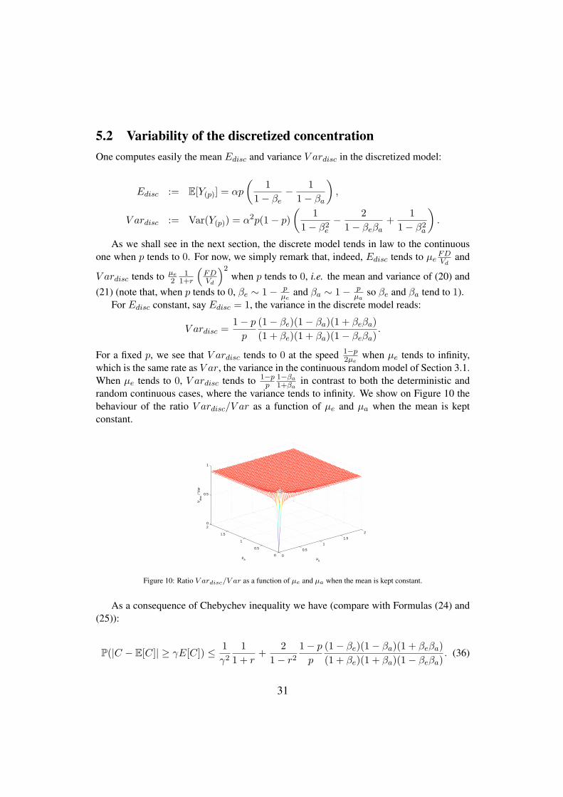
cases, where the variance tends to infinity. Figure 10 displays the evolution of the ratioV ardisc/V ar as a function of µe and µa when the mean is kept constant.
Formula (36) in Section 5.2 gives the probability that the concentration departs signif-icantly from its mean. It is interesting to compare it with (24) to contrast the impact ofnon-compliance in the discrete and continuous time models, and to (25) to measure theadded variability with respect to the fully compliant situation.
The study of the regularity of the distribution is much more involved in the discretecase than in the continuous one, as the former may display a fractal behaviour. Indeed, forsome values of the parameters, the distribution will be everywhere singular. This meansthat the evolution of the distribution varies wildly for most values of the concentration.In addition, the dichotomy smooth/singular is not governed by µ∗ alone, but by complexrelations between ke, ka and the discretization step. More precisely, the relevant parameterhere is β∗ = βe ∨βa and the regularity of the discretized model is very different dependingon whether β∗ < 1
2 or β∗ ≥ 12 .
When β∗ < 12 , the distribution of Y(p) is singular with respect to the Lebesgue measure.
This means that, in this situation, the probability distribution of the concentration will behighly irregular : it will vary erratically, taking only very particular values, and the prob-ability that it ranges in some interval varies wildly when the interval changes. Note thatβ∗ < 1
2 is equivalent to p > µ∗ log(2) or k∗ > n log(2) with k∗ = ke ∧ ka. This reflectsthe fact that, for fixed k∗, the time instants at which the patient is supposed to take his drugsare sufficiently spaced, and that he forgets to do so randomly at some of these instants.
The case β∗ > 12 is mathematically much more delicate and is not completely settled.
What is known is that the distribution of Y(p) is absolutely continuous for almost all β∗
in (12 , 1) when p = 12 : in effect, this means that the distribution of the concentration has
a probability density and thus we are in the usual situation where the probability that theconcentration ranges in some interval varies smoothly when the interval changes.
See Section 5.4 for more details.
2.6 Discrete model with random intake instants and randomdosesSimilarly to Section 2.4, we consider a random dose variant of the previous model. Thesteady state concentration now reads:
Y rd(p) = α
∞∑j=0
(βje − βj
a)DjXj , (18)
which accounts for the fact that the stochastic dose at time j/n is equal to 0 or DDj , wherethe random variables Dj are i.i.d. with mean 1 and take values in an interval [dm, dM ] with
19

0 < dm < dM < ∞. The mean Erddisc and variance V arrddisc in the random-dose discretized
model are given by (see Section 6):
Erddisc = αp
(1
1− βe− 1
1− βa
)= Edisc,
V arrddisc =
(Var(D1)
1− p+ 1
)V ardisc.
Random-dosing thus results in multiplying the variance of the deterministic-dose dis-cretized model by Var(D1)
1−p + 1. It is then easy to study the variability of the random-dosediscretized model using the analysis developed in Section 5.2 for the discretized model.
We do not have at this time any significant result concerning the regularity of the distri-bution of the concentration in this model.
This ends the overview of our models and their main features. The reader will find inthe next sections the precise derivations of the results mentioned above, along with a moredetailed analysis of the models.
3 Continuous model with random intake instants anddeterministic dosesIn this section we study the main properties of the random concentration given by (13),which we recall here for convenience:
C(t) =FD
Vd
kaka − ke
∑i
(e−ke(t−Ti) − e−ka(t−Ti)
)1l(t≥Ti),
where (Ti)i∈N is a homogeneous Poisson process with parameter λ. The probability distri-bution of C(t) may be described through its characteristic function φt. It is easily obtainedby applying Campbell’s theorem [9]. In our case, this yields:
φt(θ) = exp
{λ
∫ t
0
(exp
{iθα
(e−ke(t−x) − e−ka(t−x)
)}− 1)dx
}×exp
{iθα
(e−ket − e−kat
)}.
where we recall that α := FDVd
kaka−ke
.The change of variable u = e−(t−x) leads to:
Proposition 1. The characteristic function of C(t) is
φt(θ) = exp
{λ
∫ 1
e−t
exp{iθα
(uke − uka
)}− 1
udu+ iθα
(e−ket − e−kat
)}. (19)
20

3.1 Variability of the concentrationThe characteristic function allows us to compute the mean and variance of C(t):
E(C(t)) = λα
(1− e−ket
ke− 1− e−kat
ka
)+ α
(e−ket − e−kat
),
so that, in the long term,
limt→∞
E[C(t)] = µeFD
Vd, (20)
Likewise, the variance of C(t) reads:
Var(C(t)) = λα2
(1− e−2ket
2ke+
1− e−2kat
2ka− 2
1− e−(ka+ke)t
ka + ke
),
from which one gets
V ar = limt→∞
Var(C(t)) =µe
2
1
1 + r
(FD
Vd
)2
, (21)
with r := keka
.Note that the convergence in (20) and (21) are exponential: only a few cycles are needed
before the steady state is reached. The same remark applies to all convergences below.In the next section, we show that, when t tends to infinity, C(t) also converges to a well
defined random variable, denoted C, and we investigate in details some of its properties.Before, let us give a final result of interest pertaining to the variability of the concentrationin the non-compliant case. More precisely, the following proposition yields bounds on theprobability that the concentration exceeds a given (large) level, or departs significantly fromits mean.
Proposition 2. For γ large enough,
P(C(t) ≥ γ) ≤ 7
6γ2
(FD
Vd
)2( µe
µe − µa
)2
H(t, ke, ka, µe, µa), (22)
P(C ≥ γ) ≤ 7
6γ2
(FD
Vd
)2
µ2e
(1 +
1
2(µe − µa)
). (23)
P(|C − E[C]| ≥ γE[C]) ≤ 1
2µeγ21
1 + r. (24)
where
H(t, ke, ka, µe, µa) =[(µe − 1)
(1− e−ket
)− (µa − 1)
(1− e−kat
)]2+[µe
2
(1− e−2ket
)− µa
2
(1− e−2kat
)].
21

Proof. This is a direct application of the classical bound (see, e.g. [12], p. 209):
P(C(t) ≥ γ) ≤ 7γ
∫ 1γ
0(1−Re(φt(θ))) dθ,
valid for γ > 0, and where Re denotes the real part. Indeed,
Re(φt(θ)) = cos
(θα(e−ket − e−kat) + λ
∫ 1e−t
sin(iθα(uke−uka))u du
)× exp
{λ∫ 1e−t
cos(θα(uke−uka))−1
u du
},
and routine estimates yield (22). Inequality (23) follows in a similar way. Finally, (24) issimply Chebychev inequality.
Note that, in the deterministic case (full compliance), and with the same definition ofthe variance given by (7) in Section 2.1, one has in place of (24):
P(|Cd(t)− E[Cd]| ≥ γE[Cd]) ≤1
2µeγ2
[1
1 + r+G(r)
], (25)
with G(r) given by (10). This is another quantitative way to measure by how much theprobability of differing from the mean will be larger in the non-compliant case. For in-stance, when µe tends to infinity but µa remains bounded (which implies that r tends to 0),the above bound is of the order of 1
µ2eγ
2 , and thus much smaller than the one in (24). Whenµa tends to infinity but µe remains bounded (i.e. r tends to infinity), the bound is of theorder of 1
µ2aγ
2 , again much smaller than the one in (24). Finally, when µe and µa tend to
infinity at the same rate, the bound in the deterministic case is of the order of 1µ4eγ
2 . Thiswas illustrated on Figure 3.
3.2 Regularity of the limit distributionIn this section, we study the long term behavior of the drug concentration, that is, thedistribution function of the limit C := limt→∞C(t), where the limit is taken in the senseof convergence in distribution.
Proposition 3. The random variable C(t) converge in distribution, when t tends to infinity,to a well define random variable C whose characteristic function is
φ(θ) = exp
{λ
∫ 1
0
exp{iθα
(uke − uka
)}− 1
udu
}. (26)
Proof. When t tends to infinity, φt tends pointwise to φ, which is continuous at θ = 0. ByLevy’s theorem, this implies the result.
22

Note that the distribution of C invariant by time reversal: looking “backwards” in time,one see that C(t) has the same law as
C ′(t) =FD
Vd
kaka − ke
∑i
(e−keTi − e−kaTi
)1l(t≥Ti);
as t tend to infinity, the random variables C ′(t) converge almost surely to
C ′ =FD
Vd
kaka − ke
∑i
(e−keTi − e−kaTi
),
which therefore has the same distribution as C. In the sequel, we shall write
C =FD
Vd
kaka − ke
∑i
(e−keTi − e−kaTi
),
since we are only interested in distributional properties.
Proposition 4. The characteristic function φ satisfies
|φ(θ)| ∼ K|θ|−µ∗, when θ → ∞,
with K a positive constant and µ∗ = λ(ke∧ka) = max{µe, µa}.
Proof. One computes:
|φ(θ)| = exp
{−λ
∫ 1
0
1− cos(θα(uke − uka
))u
du
}=: exp {−λI(θ)} .
Set 0 < δ < 1, and decompose the integral I(θ) as follows:
I(θ) = I1(θ)− I2(θ)− log(δ), (27)
where
I1(θ) =
∫ δ
0
1− cos(θα(uke − uka
))u
du,
I2(θ) =
∫ 1
δ
cos(θα(uke − uka
))u
du.
(28)
When 0 ≤ u ≤ δ, we have that α(uke − uka
)∼ |α|uke∧ka , and thus
I1(θ) ∼∫ δ
0
1− cos(θαuke∧ka
)u
du
∼ 1
ke ∧ kalog(θ|α|) + γe
ke ∧ ka+ log(δ) +O
(1
θ
),
(29)
23

where γe is the Euler constant.
Denote h(u) = α(uke − uka
). The function h has a global maximum at u0 =
(keka
) 1ka−ke
with h”(u0) < 0. Stationary phase arguments imply that, when θ tends to infinity,
I2(θ) ∼ Re
(∫ 1
δ
eiθα(uke−uka )
udu
)
∼ Re
(ei(θh(u0)−π/4)
√2π
u0√
θ|h”(u0)|
)
=cos(θh(u0)− π/4)
u0
√2π
θ|h”(u0)|
= O
(1√θ
).
(30)
Formulas (27), (28), (29) and (30) entail that
I(θ) =1
ke ∧ kalog(θ|α|) + γe
ke ∧ ka+O
(1√θ
).
This implies that there exists K > 0 such that |φ(θ)| ∼ K|θ|−µ∗when θ tend to infinity.
We denote by F the probability distribution function of C, associated to φ. Then, fromProposition 4 we have the following results with respect to the regularity of F :
1. F has an L2 density1 if and only if µ∗ > 12 .
2. For µ∗ < 1 and 0 < ε < 1,∫∞1 θµ
∗−ε|φ(θ)|dθ < ∞ thus F ∈ Lip(µ∗ − ε).
3. For µ∗ < 12 , 1
T
∫ T−T |φ(θ)|2dθ = O
(T−2µ∗)
thus F ∈ Lip(µ∗).
4. A classical Tauberian theorem (see, e.g. [7], p.445) entails that:
F (ε) ∼ e−µ∗γe |α|−µ∗
Γ(µ∗ + 1)|ε|−µ∗
,
when ε → 0. Then, F is not differentiable at 0 when µ∗ < 1 and it has a finite nonvanishing derivative at 0 exactly when µ∗ = 1.
5. From Proposition 3 in [11], we have that, for any x > 0,
F (x+ ε)− F (x) = O(ε),
when ε → 0+. This implies that 0 is the only possibly singular point of F .
1This means that the integral of the square of the probability density function is finite.
24

The practical meaning of these results is that, when λ < min{ka, ke} the instant ofintakes are too scarce, with respect to the absorption and the elimination rates, resulting ina high probability of having too small concentration of drugs.
4 Continuous model with random intake instants andrandom dosesIn this section, we consider the generalization of the continuous model of Section 3 to allowfor random doses. We study the main properties of the random concentration Crd(t), givenby (16), which we recall here for convenience:
Crd(t) =FD
Vd
kaka − ke
∑i
Di
(e−ke(t−Ti) − e−ka(t−Ti)
)1l(t≥Ti),
where the (Ti)i∈N again form a Poisson process, and the (Di)i∈N are random variables. Fand Vd are constants. At time Ti, the dose taken is DDi, and we assume that E(Di) = 1,that Di is supported on R+, and that it has compact support (although we shall need onlyweaker assumptions).
The process Crd(t) thus defined is a marked Poisson process. In this work, we shall as-sume that the (Di)i∈N are independent and identically distributed random variables, whereeach Di may depend on Ti but is independent from the (Tj)j =i. This makes sense froma pharmacokinetic point of view, since it seems plausible that the patient will not adjusthis dose at time Ti on the basis of his past or future behavior except for the time lag fromthe previous take, although it would maybe be desirable to let Di depend also on Di−1.We denote by ν(T, .) the conditional distribution of Di knowing that Ti = T . Our as-sumptions allow to apply a generalized form of Campbell theorem [9] to the effect that thecharacteristic function φrd
t of Crd(t) is given by:
φrdt (θ) = exp
{λ
∫ t
0
∫A
(eiθαuh(t−x) − 1
)ν(x, du)dx+ iθαh(t)
}(31)
where, as before, α = FDVd
kaka−ke
, h(t) = e−ket − e−kat and A is the support of the Di.
4.1 Variability of the concentrationFrom (31), one deduces easily the mean and variance of Crd:
(φrdt )′(θ) = φrd
t (θ)
[λ
∫ t
0
∫Aiαuh(t− x)eiθαuh(t−x)ν(x, du)dx+ iαh(t)
],
and thus
(φrdt )′(0) = iα
(µe(1− e−ket)− µa(1− e−kat)
)Ex(D1) + iα
(e−ket − e−kat
).
25

where Ex(D1) =∫A uν(x, du) is the expectation of Di knowing that Ti = x, which is
equal to one for any x by assumption. Thus we find that, not surprisingly:
E(Crd(t)) = E(C(t)).
Likewise,
(φrdt )”(θ) = φrd
t (θ)
[(λ
∫ t
0
∫Aiαuh(t− x)eiθαuh(t−x)ν(x, du)dx− α2h2(t− x)
)2
−λ
∫ t
0
∫Aα2u2h2(t− x)eiθαuh(t−x)ν(x, du)dx
].
Using that, by definition,∫A u2ν(x, du) = Ex[D
21], this entails:
(φrdt )′′(0) = −E[C(t)]2 − λα2
∫ t
0h2(t− x)
∫Au2ν(x, du)dx
= −E[C(t)]2 − λα2
∫ t
0h2(t− x)Ex(D
21)dx
or, since (φrdt )′′(0) = −E[C(t)]2 −Var(Crd(t)),
Var(Crd(t)) = λα2
∫ t
0h2(t− x)Ex[D
21]dx.
However,Ex(D
21) = Varx(D1) + Ex[D1]
2 = Varx(D1) + 1
(Varx(D1) denotes the variance of Di knowing that Ti = x) and
λα2
∫ t
0h2(t− x)dx = Var(C(t)),
thus
Var(Crd(t)) = Var(C(t)) + λα2
∫ t
0h2(tx)Varx(D1)dx.
Assuming that Varx(D1) = Var(D1), i.e. the variance of Di does not depend on the valueof Ti, one gets:
Var(Crd(t)) = E[D21]Var(C(t)) = (1 + Var(D1))Var(C(t)).
Thus random-dosing results in multiplying the variance of the deterministic-dose case byE(D2
1). It is then easy to obtain inequalities similar to (22), (23) and (24) for the random-dose case.
Two particular cases may be of special interest:
26

• Discrete distribution: the Di assume the values {d1, . . . , dm} ⊂ R+ with probabili-ties q1, . . . , qm, independently of the Ti. We denote by Crd,d
t and φrd,dt the concen-
tration and characteristic function. Then:
φrd,dt (θ) =
m∏j=1
φt(qjλ, djθ), (32)
where we have written φt(qjλ, ·) instead of φt(.) for the characteristic function in thedeterministic-dose case, given in equation (19), but with parameter qjλ instead of λ.This equality also holds when t tends to infinity, yielding the long term concentrationcharacteristic function. The variance is given by:
Var(Crd,d(t)) = E[D21]Var(C(t)) =
m∑j=1
qjd2j
Var(C(t)).
It is of interest to characterize the situation giving the largest variance among alladmissible random dosings with arbitrary m, qi, and di. In other words, we look forthe value of Vmax := max{Var(Crd,d(t))} subject to m > 1, (q1, . . . , qm) ∈ [0, 1]m
with at least two qi non zero and∑m
j=1 qi = 1, (d1, . . . , dm) ∈ [a, b] with b > a > 0,and
∑mj=1 qidi = 1. It is easily shown, for instance using Lagrange multipliers, that
the maximum is reached for m = 2 and d1 = a, d2 = b. In this case,
Vmax = (a+ b− ab)Var(C(t)). (33)
Thus the worst-case situation is when the patient “oscillates” between two dosingswhose average is the prescribed one.
• Uniform distribution: the Di are uniformly distributed over [a, b] ⊂ R+, indepen-dently of the Ti. We denote by Crd,u
t and φrd,ut the concentration and characteristic
function. In this case, one computes:
φrd,ut (θ) = exp
{λ
b− a
∫ b
a
∫ 1
e−t
eiθyα(uke−uka ) − 1
ududy + iθαh(t)
}. (34)
This last function is easily seen to be convergent when t tends to infinity, whichgives us the long term concentration characteristic function. Note that φrd,u tendsto φ when the couple (a, b) tends to (D,D): the concentration with random dosesuniformly distributed on [a, b] tends in law to the concentration with fixed dose D.The variance is given by:
Var(Cu(t)) = E(D21)Var(C(t)) =
a2 + ab+ b2
3Var(C(t)). (35)
We can see that the choice of [a, b] maximizing the variance under the constraintE(D1) = 1 is a = 0, b = 2, as expected.
27

4.2 Regularity of the limit distributionWe first consider the two cases of discrete and uniform random dosing.
• Discrete distributionFrom (32) and Proposition 4, one easily sees that:
|φrd,d(θ)| ∼m∏j=1
(djθ)−qjµ
∗= Kθ−µ∗
when θ tends to infinity, where K is a constant.
• Uniform distributionIn this case, the limit of the function φrd,u
t , defined in Formula (34), when t tends toinfinity is:
φrd,u(θ) = exp
{λ
b− a
∫ b
a
∫ 1
0
eiθyα(uke−uka ) − 1
ududy
}.
The modulus of φrd,u is
|φrd,u(θ)| = exp
{−λ
(b− a)
∫ b
a
∫ 1
0
1− cos(θyα(uke − uka))
ududy
},
= exp
{−λ
(b− a)
∫ b
aI(θy)dy
}.
The proof of Proposition 4 shows that, for large enough θ,
I(θy) ∼ 1
ke ∧ kalog(θy|α|) + constant.
This implies that there exists K > 0 such that |φ(θ)| ∼ K|θ|−µ∗when θ tends to
infinity. This fact will be justified in the proof of Proposition 5.
Thus in both particular cases above, we recover the same behaviour for the characteristicfunction as in the deterministic-dose case. As the next proposition shows, this is in fact ageneral feature of all random dosings provided ν(x, du) does not depend on x, with anadditional mild condition:
Proposition 5. Assume that ν(x, du) = ν(du) and that∫A log(y)ν(dy) < ∞. Then
|φrd(θ)| ∼ K|θ|−µ∗
when θ tends to infinity, where K is a positive constant.
28

Proof. Thanks to the assumption on ν, one computes
|φrd,u(θ)| = exp
{−λ
∫A
∫ 1
0
1− cos(θyα(uke − uka))
uduν(dy)
}= exp
{−λ
∫AI(θy)ν(dy)
}.
The proof of Proposition 4 shows that, when θ tends to infinity,
−λI(θy) ∼ K − µ∗(log(θ) + log(y))
for a certain constant K, with in addition −λI(θy)−K + µ∗(log(θ) + log(u)) tending to0 with a rate of convergence 1√
θ. Thus, using the assumption on the logarithmic moment of
ν,
−λ
∫AI(θy)ν(dy) ∼ K − µ∗ log(θ)− µ∗
∫Alog(y)ν(dy)
and one finishes up the proof with the help of a dominated convergence argument to showthat the difference between the right-hand side and the left-hand side in the equivalent aboveindeed tends to 0 when θ tends to infinity.
Proposition 5 shows that random dosing, at least when the distribution of the Di isindependent of the Ti, does not alter the regularity of the distribution of the long-termconcentration as compared to the deterministic-dose case.
5 Discrete model with random intake instants anddeterministic dosesWe study in this section a discretization in time of the model above. In other words, insteadof taking the drug at arbitrary time instants t ∈ R+, we assume that the patient will only doso at (random) times which form a subset of {tnl = l/n; l ∈ N}, where n is a fixed number.We shall first rewrite the drug concentration in this discrete setting. It will appear that thediscretized concentration Cd has the same law as an object that has been thoroughly studiedin mathematics under the name of infinite Bernoulli convolution. We will study the vari-ability of the discretized concentration. Then we will show that, when n tends to infinity,the discretized model indeed tends distribution-wise to the continuous-time one. We willfinally study the regularity of the long term behaviour of the discretized concentration forn fixed or tending to infinity, and show that it is, under certain circumstances, singular.
5.1 The discretized concentrationThe discretized model taking the following form. Let h = 1
n be the discretization step.Thus, the drug intakes can only occur at times tj = jh with j ∈ N.
29

From a general point of view, the discrete analog of the Poisson process is the Bernoulli pro-cess. Indeed, in the continuous framework, the Poisson process is the only counting processwhich has stationary and independent increments. Likewise, the only discrete counting pro-cess with the same property is the Bernoulli process. In terms of waiting times, this amountsto replacing the i.i.d., memoryless, exponential random variables Sn = Tn+1−Tn, by i.i.d.random variables following a geometric distribution (recall that the geometric distributionis the only memoryless discrete distribution).
We are thus led to consider a sequence (Xj)j∈N of i.i.d. Bernoulli random variableswith parameter p such that Xj = 1 if the patient takes the drug at time tj and Xj = 0 ifnot.
In this discrete model the number of drug intakes per unite time is ph , so one has choose
p = λh. Note that, for the model to make sense, p must be smaller than one, whichtranslates into λh < 1.
At a fixed time tn the contribution of the j-th intake to the current concentration is
α(βn−je − βn−j
a
)Xj ,
where βe = e−keh and βa = e−kah: βe is the elimination rate for one time step and βa isthe absorption rate for one time step.
Thus, the total concentration at time tn is given by
Cn = α
n∑j=0
(βn−je − βn−j
a
)Xj .
Since the random variable (Xj)j∈N are independent, they are exchangeable, and in par-ticular the vector (X0, . . . , Xn) has the same distribution as the reversed vector (Xn, . . . , X0).Hence Cn is equal in distribution to
Yn = α
n∑j=0
(βje − βa
j)Xj .
The sequence (Yn) converges almost surely to the random variable Y(p), given by equa-tion (17) in Section 2.5; i.e.,
Y(p) = α∞∑j=0
(βje − βa
j)Xj .
The distribution of Y(p) is thus the one of the long term concentration in this model.Since Y(p) is an infinite sum of independent Bernoulli random variables, its law is an infiniteconvolution of Bernoulli distribution, hence its name “infinite Bernoulli convolution”.
From the independence of (Xj)j∈N we have that the characteristic function of Y(p) isgiven by
φp(θ) =
∞∏j=0
[(1− p) + peiθα(β
je−βj
a)].
30
5.2 Variability of the discretized concentrationOne computes easily the mean Edisc and variance V ardisc in the discretized model:
Edisc := E[Y(p)] = αp
(1
1− βe− 1
1− βa
),
V ardisc := Var(Y(p)) = α2p(1− p)
(1
1− β2e
− 2
1− βeβa+
1
1− β2a
).
As we shall see in the next section, the discrete model tends in law to the continuousone when p tends to 0. For now, we simply remark that, indeed, Edisc tends to µe
FDVd
and
V ardisc tends to µe
21
1+r
(FDVd
)2when p tends to 0, i.e. the mean and variance of (20) and
(21) (note that, when p tends to 0, βe ∼ 1− pµe
and βa ∼ 1− pµa
so βe and βa tend to 1).For Edisc constant, say Edisc = 1, the variance in the discrete model reads:
V ardisc =1− p
p
(1− βe)(1− βa)(1 + βeβa)
(1 + βe)(1 + βa)(1− βeβa).
For a fixed p, we see that V ardisc tends to 0 at the speed 1−p2µe
when µe tends to infinity,which is the same rate as V ar, the variance in the continuous random model of Section 3.1.When µe tends to 0, V ardisc tends to 1−p
p1−βa
1+βain contrast to both the deterministic and
random continuous cases, where the variance tends to infinity. We show on Figure 10 thebehaviour of the ratio V ardisc/V ar as a function of µe and µa when the mean is keptconstant.
0
0.5
1
1.5
2
0
0.5
1
1.5
20
0.5
1
µe
µa
Vdi
sc /
Var
Figure 10: Ratio V ardisc/V ar as a function of µe and µa when the mean is kept constant.
As a consequence of Chebychev inequality we have (compare with Formulas (24) and(25)):
P(|C − E[C]| ≥ γE[C]) ≤ 1
γ21
1 + r+
2
1− r21− p
p
(1− βe)(1− βa)(1 + βeβa)
(1 + βe)(1 + βa)(1− βeβa). (36)
31

5.3 Limit when the discretization step tends to 0The following proposition describes the behaviour of Y(p) when n tends to infinity or, whichis the same, when p tends to zero. Note that this also equivalent to letting βe and βa tend to1.
Proposition 6. Y(p) converges in law to C when p tends to zero.
Proof. The proof is analogous to the one of Proposition 4 in [11]: one shows that thecharacteristic function φp of Y(p) tends pointwise to the characteristic function φ of C. Thedetails are omitted.
In practical terms, this results means that, as long as we are only interested in distribu-tional properties of the concentration, we may consider the discrete model instead of thecontinuous one provided p is chosen small enough. Note however that the discrete modelwith arbitrary value of p is interesting in its own right.
5.4 Regularity of the discretized modelWe assume that µa = µe, since Y(p) is constantly equal to zero when µa = µe. The work[1] provides an analysis of the regularity of generalized infinite Bernoulli convolutions, andspecially its fractal properties. The interested reader may also consult [6, 16, 17] for studieson regular infinite Bernoulli convolutions.
The relevant parameter here is β∗ = βe ∨βa. The results of [1] show that the regularityof the discretized model is very different depending on whether β∗ < 1
2 or β∗ ≥ 12 :
• When β∗ < 12 , the distribution of Y(p) is singular with respect to the Lebesgue mea-
sure. More precisely, the Hausdorff dimension of its support is equal to
lim infn→∞
−n log(2)
log(ρn)=
log(2)
log(β∗)< 1,
where ρn = α(βn+1e
1−βe− βn+1
a1−βa
). The Hausdorff dimension measures the “size”, in a
certain sense, of the support of the measure, i.e. where it is concentrated. A Haus-dorff dimension smaller than one means that the set of possible values taken by theconcentration is extremely sparse and does not form a continuum. In addition, theprobability of being in an interval varies in a very non-smooth way with the boundsof the interval. In practical terms, this means that probability distribution of the con-centration will be highly irregular : it will vary erratically, taking only very particularvalues, and the probability that it ranges in some interval may vary wildly when theinterval changes. Note that β∗ < 1
2 is equivalent to p > µ∗ log(2) or hk∗ > log(2)with k∗ = ke ∧ ka, (recall that h is the discretization step ). This reflects the fact that,for fixed k∗, the time instants at which the patient is supposed to take his drugs aresufficiently spaced, and that he forgets to do so randomly at some of these instants.
32

Alternatively, for a fixed h, k∗ must be sufficiently large. Note also that, in view ofp < 1, this is possible only if µ∗ < 1
log(2) .
• The case β∗ > 12 is mathematically much more delicate and is not completely settled.
Results given in [5, 15] entail that the distribution of Y(p) is absolutely continuous forLebesgue-almost all β∗ in (12 , 1) when p = 1
2 . This means that the distribution ofthe concentration has a probability density: in other words, in contrast with the caseβ∗ < 1
2 , we are in the usual situation where the probability that the concentrationranges in some interval varies smoothly when the interval changes.
• In all other cases, the characterization of the regularity of the distribution of Y(p)remains an open problem.
6 Discrete model with random intake instants andrandom dosesIn the discrete case, the random-dose model takes the following form:
• We still have a sequence of i.i.d. Bernoulli random variables (Xj)j≥0 with parameterp, which mark the random instants of drug intake.
• To account for the random dosing, we consider a sequence of i.i.d. random variables(Dj)j≥0, that will represent the doses, with distribution ν compactly supported onR∗+. We will let ν denote the product measure ν
⊗N.
• We make the assumption E[D1] = 1, which means that the patient takes the normaldose on average.
• We suppose that all the Di are independent of the Xj .
• As before, βe = e−keh and βa = e−kah are respectively the elimination rate and theabsorption rate for one time step.
We investigate the behaviour of the almost sure limit (with respect to ν) of the steadystate concentration Y rd
(p), given by Formula (18) in Section 2.6, i.e.
Y rd(p) = α
∞∑j=0
(βje − βj
a)DjXj .
Independence of (Xj)j∈N and (Dj)j∈N entail that the characteristic function of Y rd(p) is
given by
φrdp (θ) =
∞∏j=0
[(1− p) + p
∫eiθα(β
je−βj
a)uν(du)
].
As before, we first proceed to investigate the variability in this model, and then thelimit when the discretization step tends to zero. We do not characterize the regularity of theconcentration, as no results are available in this more complex situation.
33

6.1 Variability of the concentrationThe mean Erd
disc and variance V arrddisc in the random-dose discretized model are easily seento be:
Erddisc := E[Y rd
(p)] = αp
(1
1− βe− 1
1− βa
)= Edisc,
V arrddisc := Var(Y rd(p)) = α2 (Var(D1)p+ p(1− p))
(1
1− β2e
− 2
1− βeβa+
1
1− β2a
)=
(Var(D1)
1− p+ 1
)V ardisc.
Random-dosing thus results in multiplying the variance of the deterministic-dose dis-cretized model by Var(D1)
1−p + 1. It is then easy to study the variability of the random-dosediscretized model using the analysis developed in Section 5.2 for the discretized model.
6.2 Limit when the discretization step tends to 0The following result can be proved in the same way as Proposition 4 in [11]:
Proposition 7. Y(p) converges in law to Crd when p tends to zero.
Again, this means that, if one is only interested in distributional properties of the con-centration, the discrete model may be considered in place of the continuous one provided pis chosen small enough.
AcknowledgementsThe research of L.J. Fermın was supported by Proyect DIGITEO DIM, ANIFRAC : Un-certaities in processes with fractal characteristics, and by a research grant from the ProyectDIUV N◦ 2/2011 of the University of Valparaıso.
References[1] Albeverio, S., Torbin, G. (2008). On fine fractal properties of generalized infinite
Bernoulli convolutions. Bull.Sci. Math. 132: 711–727.
[2] Barriere, O., Jun, L., Fahima, N. (2011). A Bayesian approach for the estimationof patient compliance based on the last sampling information. Journal of Phar-macokinetics and Pharmacodynamics 38 (3):333–351.
34

[3] Barriere, O., Jun, L., Fahima, N. (2013). Compliance spectrum as a drug fin-gerprint of drug intake and drug disposition. Journal of Pharmacokinetics andPharmacodynamics 40 (1): 41–52.
[4] Fermin, L., Levy Vehel, J. Modeling patient poor compliance in the multi-IVadministration case with Piecewise Deterministic Markov Models, preprint.
[5] Cooper, M. (1998). Dimension, measure and infinite Bernoulli convolutions,Math. Proc. Cambr. Phil. Soc. 124: 135–149.
[6] Erdos, P. (1939). On a family of symmetric Bernoulli convolutions, Amer. J. Math.61: 974–975.
[7] Feller, W. (1971). An introduction to probability theory and its applications, Vol.II, 3rd edition, Wiley.
[8] Gaudreault, F., Drolet, P., Fallaha, M. and Varin, F. (2012). A population pharma-cokinetic model for the complex systemic absorption of ropivacaine after femoralnerve block in patients undergoing knee surgery. Journal of Pharmacokinetics andPharmacodynamics. 39 (6): 635–642.
[9] Kingman, J.F.C. (1993). Poisson Processes, Oxford University Press, Oxford.
[10] Iskedjian, M., Einarson, T.R., MacKeigan, L.D., Shear, N., Addis, A., Mittmann,N., and Ilersich, A.L. (2002). Relationship between daily dose frequency andadherence to antihypertensive pharmacotherapy: evidence from a meta-analysis.Clin. Ther. 24 (2), 302–316.
[11] Levy Vehel, P.E, Levy Vehel, J. (2012). Variability and singularity arising frompoor compliance in a pharmacokinetic model I: the multi-IV case. Journal ofPharmacokinetics and Pharmacodynamics 40 (1):15–39.
[12] Loeve, M.(1977). Probability Theory I, Fourth Edition, Springer Verlag.
[13] Li, J. and Nekka, F. (2006). A Pharmacokinetic Formalism Explicitly Integratingthe Patient Drug Compliance. J. Pharmacokinet. Pharmacodyn. 34 (1), 115–139.
[14] Li, J. and Nekka, F. (2009). A probabilistic approach for the evaluation of phar-macological effect induced by patient irregular drug intake. J. Pharmacokinet.Pharmacodyn. 36: 221–238.
[15] Pratsiovytyi, M. and Torbin, G. (1998). A class of random variables of theJessen-Wintner type. Proceedings of the Ukrainian National Academy of Sciences(Dopovidi Nat. Acad. Nauk). 4: 48–54.
[16] Peres, Y., Schlag, W., Solomyak, B. (2000). Sixty years of Bernoulli convolutions.Fractal geometry and stochastics, II (Greifswald/Koserow, 1998), Progr. Probab.,Birkhauser, Basel, 46: 39–65.
[17] Peres, Y. and Solomyak, B. (1996). Absolute Continuity of Bernoulli Convolution,a Simple Proof. Math. Res. Lett. 3 (2): 231–239.
35

[18] Sheiner L.B., Rosenberg B., Marathe V.V. (1977). Estimation of population char-acteristics of pharmacokinetic parameters from routine clinical data. J. Pharma-cokinet Biopharm. 5 (5):445-79.
[19] Widmer, N. et al. (2006). Population pharmacokinetics of imatinib and the role ofα1-acid glycoprotein. British Journal of Clinical Pharmacology. 62 (1):97–112.
36