value of travel time savings
TRANSCRIPT

i
Value of Travel Time Savings A study in the cross-mode variations of mixed logit estimates
Ioannis Tikoudis
Master thesis for the M.Phil in Environmental and Development Economics
UNIVERSITY OF OSLO
August 2008

i
Acknowledgements
This study was carried out in the Norwegian Institute of Transport Economics TØI
(Transportøkonomisk institutt), with the financial support of the Norwegian Public Roads
Administration (Statens vegvesen).
I would like to express my gratitude to my supervisor and teacher Farideh Ramjerdi for her
indispensable guidance, her constant motivation, for providing me with a rich database and for
trusting me to undertake a really challenging topic in TØI.
Also, I am grateful to James Odeck and the National Public Roads Administration for the
financial assistance. I would also like to warmly thank John Dagsvik, Tore Schweder and Tapas
Kundu for their technical advices.
Finally, thanks to friends Mike Lowry and Svenn Jensen for their support and the nice
discussions we had in TØI.

ii
Table of Contents Value of Travel Time Savings ..................................................................................................................... i
0. Introduction ......................................................................................................................................... 1
0.1 The value of travel time savings (VTTS) ........................................................................................... 1
0.2 Problem statement ........................................................................................................................ 2
0.3 Relevant literature and contribution from this study ...................................................................... 3
0.4 Structure of the thesis .................................................................................................................... 3
1. Theoretical underpinnings of VTTS ....................................................................................................... 6
1.1 Becker ............................................................................................................................................ 6
1.2 DeSerpa ......................................................................................................................................... 8
1.3 Discrete choice models and VTTS ................................................................................................... 9
2. Data ................................................................................................................................................... 11
2.1 Advantages and Shortcomings of Revealed preference data. ........................................................ 11
2.2 Stated Preference data ................................................................................................................. 12
2.3 Sampling and data set. ................................................................................................................. 14
2.4 Design of choice experiments ....................................................................................................... 16
3. Discrete choice and Random Utility models........................................................................................ 18
3.1. Framework set up for a deterministic choice theory .................................................................... 18
3.2. Random Utility Models ................................................................................................................ 18
3.3. Binary logit .................................................................................................................................. 20
3.4. Mixed logit .................................................................................................................................. 23
3.5. Binary probit ............................................................................................................................... 25
4. VTTS estimations ............................................................................................................................... 26
4.1. Estimation of VTTS with Logit specification .................................................................................. 26
4.2. Do we really need Mixed Logit? ................................................................................................... 30
4.3. Which parameters should be random? ........................................................................................ 33
4.4. Which ‘mixing distribution’ to use? ............................................................................................. 33
4.5. Normally distributed time coefficient .......................................................................................... 35
4.6. Log-Normally distributed time coefficient ................................................................................... 39
4.8 Johnson SB distributed time coefficient ........................................................................................ 43
4.9 Johnson SB with fixed upper bound .............................................................................................. 46

iii
5. Socioeconomic segmentation of VTTS ................................................................................................ 49
5.1 A model with income segmentation ............................................................................................. 49
5.2. A model with gender ................................................................................................................... 52
6. Sources of variation ........................................................................................................................... 54
6.1 Distinguishing the effects ............................................................................................................. 54
6.2. User type effects ......................................................................................................................... 56
6.3. Mode effects and strategic behavior ........................................................................................... 57
7. Concluding remarks and future challenges ......................................................................................... 61
Appendix A: Likelihood Ratio tests ......................................................................................................... 64
References ............................................................................................................................................. 65

iv
List of abbreviations
CE………………..Choice experiments
CV……………….Contingent Valuation
GLR……………...Generalized Likelihood Ratio
IIA……………….Independence of Irrelevant Alternatives
L…………………Alternative on the Left side of the respondent’s screen (Refers always to the
first alternative of the binary choice set)
LM……………… Lagrange Multiplier
LR………………..Likelihood Ratio
ML……………….Maximum Likelihood
MLE……………..Maximum Likelihood Estimate
MSL……………..Maximum Simulated Likelihood
NOK…………….Norwegian Kroner
pdf……………….Probability distribution function
R………………... Alternative on the Right side of the screen (Refers always to the second
alternative of the binary choice set)
RP………………. Revealed Preference
RUM…………… Random Utility Model
SP………………. Stated Preference
TT……………….Travel time
VoT ……………...Value of time
VTT…………….. Value of Travel Time
VTTS…………… Value of Travel Time Savings
WTP…………….Willingness to Pay

1
0. Introduction
0.1 The value of travel time savings (VTTS)
The value of travel time savings (VTTS) is the monetary value attached to reductions in
travelling time. “With some exception, travel is considered as an intermediate good. Hence it is
the travel time savings that should constitute value” (Ramjerdi, 1993). Unfortunately there is
neither a market, nor an observable price for time. Nevertheless, people are willing to pay for
time savings; in most economic decisions time is present, at least in the background.
VTTS is an important willingness-to-pay (WTP) indicator which plays a crucial role in economic
evaluation of transport projects and in pricing policies. ‘In the UK for example, travel time
savings have accounted for around 80% of the monetized benefits within the cost-benefit
analysis of major road schemes’ (Mackie et al., 2001). Practically, behavioral values of various
types of travel time are obtained from travel demand models as an implicit trade off between
money and travel time. VTTS is estimated from models of discrete choice as the ratio of the
marginal utility of time on the marginal utility of income. For linear-in-parameters utility
specifications this ratio is simply the ratio of time on price coefficient. There is a methodological
debate on the legitimacy of discrete choice models to estimate VTTS and on their justification by
economic theory (see Chapter 1).
Empirically, it is often the case that VTTS exhibits large variations with respect to many
parameters rather than being homogeneous across them. These can be associated with the trip
itself (trip characteristics, i.e. distance, purpose), the type of user or socioeconomic status of the
traveler (e.g. income, age, family status etc.), the attributes of the transport mode (e.g. comfort,
travel fare), etc.
Ramjerdi (1993) summarizes the possible explanations for these variations. Concerning trip
characteristics, travel purpose is a source of VTTS variation; travel time savings when
commuting to work are usually valued higher than non-work travel time savings. With reference
to socioeconomics, income may also play a role, mainly because it is associated with the ability
to pay or act as a source of taste variation. Furthermore, VTTS is non homogenous across mode
attributes such as travel time; VTTS may not be linear in time and may vary according to the
time components of a trip. Other individual characteristics such as age may also explain some of
these variations. Thus, it is a challenging task for the researcher to separate the sources of
variation; what is practically observed is a multidimensional joint distribution of VTTS in the
above parameters with non-experimental observations, i.e. the researcher cannot perfectly
control the above covariates.

2
0.2 Problem statement
This study focuses on the variations of VTTS across transport modes for long distance, private
purpose trips in Norway. The task is to examine why different VTTS estimates are obtained for
the various transport modes. More particularly we are examining mode effects (e.g. if people
adjust their WTP for travel time savings according to the attributes of a mode, because they
perceive travelling with a particular mode a unique activity) and self selection (e.g. the observed
differences stem from the variations in individual characteristics of people, who switch to the
transport mode that best fits their WTP) as sources of variation. We also attempt to give an
insight into a third effect, namely strategic behavior. In stated preference (SP) surveys it is
highly likely that respondents have an incentive to not reveal their true WTP. This incentive
differs across modes, causing respondents to overstate their WTP for some modes and understate
it for some others.
Other sources may be exogenous to the consumer choice but specification or estimation-related,
i.e. the VTTS gaps depend on the employed method of estimation.
Investigating VTTS differences across modes is quite important in the appraisal of transport
investments. Assume that a transport project which is associated with an improvement in the
attributes of one or more transport modes is under evaluation. The before-after difference in total
benefits depends on:
• The changes in choice probabilities (changes in market shares). Since the relative levels
of attributes will change, some people will reconsider their choice of transport mode.
Therefore, some people will switch to a mode that better suits their profile (user type
effects). For example, people with high VTTS may switch to the mode that becomes
relatively faster. For example a highway car-only high speed line may induce ‘impatient’
passengers to switch to car.
• The change in VTTS for a given mode. The WTP for time savings in each mode may
change, as a result of the attribute modification (mode effects). For example, improved
environment in public transport mode may render travelling a more pleasant activity and
thus reduce WTP for time savings in that mode.
Knowing the relative impact of the two effects makes it possible to correctly predict the direction
of change in total VTTS savings, which is part of the change in total benefits in the context of
appraisal schemes. In other words, knowledge over the sources of variation is necessary to
predict variation.

3
0.3 Relevant literature and contribution from this study
A plethora of studies have been dedicated to VTTS, especially in the Western countries. Value of
Time (VoT) studies have taken place for instance in Norway (Ramjerdi et al., 1997), Sweden
(Algers et al., 1998), Denmark (Fosgerau et al., 2007) and Switzerland (König et al., 2003). The
latter provides a brief review of the available work in the field.
The Swedish study offers VTTS estimates derived with logit and mixed logit with normal mixing
distribution. Fosgerau et al. (2007) is the only work that focuses on the cross mode variations in
VTTS. Our approach uses a similar methodological basis to the Danish one, namely that it
attempts to separate mode and user type effects by forming user type groups in order to
investigate the mode impact within a user type group and the user type impact across user groups
in a given mode.
Nevertheless, the methodological basis of the Danish study has been adjusted to fit the
Norwegian experimental design and data set. Particularly, VTTS estimates used in the final
section are normally distributed in contrast to the Danish study’s, in which VTTS is directly
parametrized and modeled to follow a lognormal distribution. The exact VTTS formulations of
Fosgerau et al. (2007) do not fit the Norwegian experimental design. The experimental design
that generated the choice experiments and subsequently the Norwegian SP data set is different
than both the Danish and the Swedish corresponding ones (see Chapter 2).
Furthermore, the use of random coefficient models (mixed logit) constitutes an adoption of state-
of-the-art, recent developments in the field, allowing us to account for random taste variation.
Since the Norwegian Value of Time study (Ramjerdi et al., 1997) provided only logit estimates,
the re-estimation with various mixed logit models provides an insight into the vulnerability of
VTTS estimates to various hybrid models. In that sense, this work extends the result set of the
Norwegian VoT study.
0.4 Structure of the thesis
The thesis comprises seven chapters. Chapter 1 discusses the theoretical underpinnings of VoT.
The point of departure is the theories of optimal time allocation of Becker and DeSerpa. Some
part of the discussion is dedicated on whether discrete choice models are consistent with the
economic theory of time allocation. Attention is given to possible limitations that theory suggests
on the estimates of econometric models, e.g. negative VTTS. Theory serves mainly as a
benchmark and can (if not must) also take feedback from empirical results.

4
Chapter 2 summarizes the data used in this study. Sections 2.1 and 2.2 discuss the possible
advantages of stated preference (SP) over revealed preference (RP) data in this type of studies.
Section 2.3 describes the sampling process and the data set used in the estimations; all estimates
in this study refer to long distance trips. Section 2.4 is a brief review of the experimental design
employed to generate the binary choice experiments used in the survey.
Chapter 3 summarizes the compatible discrete choice methods that can be used in VTTS
estimation for the data set described in Chapter 2. The described methods are tailor-selected to
fit the binary choice experiments. Section 3.1 presents the basic setup of a deterministic discrete
choice model, 3.2 focuses on making discrete choice setups operational by Random Utility
theory. Sections 3.3-3.5 present binary logit, mixed logit and binary probit, the advantages and
disadvantages of each. The first two are the models used to estimate VTTS in the empirical part
of the study. We highlight the main shortcomings on logit which motivate the use of hybrid
models.
Chapters 4 to 6 constitute the empirical part of the study. Section 4.1 provides VTTS estimates
from a pure logit model, 4.2 presents a likelihood ratio test for the justification of mixed logit
model and 4.3 asserts which coefficients should be random. Estimations with random coefficient
models have been carried out with three different mixing distributions. Section 4.4 discusses the
behavioral implications for each of them and sections 4.5-4.8 provide estimation results with
normal, lognormal and Johnson SB mixing distribution. A brief conclusion of this chapter is that
estimates are highly sensitive to the assumption of mixing distribution.
Chapter 5 provides a socio-economic segmentation of VTTS. Section 5.1 investigates the
relationship between income and VTTS and section 5.2 introduces gender in the analysis.

5
Chapter 6 investigates the effect of three possible sources of variation, namely user type effects,
mode effects and strategic behavior. We argue that, in contrast to the clear evidence of the
Danish study, Norwegian data do not reveal any of these effects to be dominant. It seems
however that user type effects and strategic behavior are more evident than mode effects. Finally,
Chapter 7 highlights the most important findings and poses the challenges for future research. A
summary of the study’s structure is presented in Figure A.

6
1. Theoretical underpinnings of VTTS
The VTTS is the amount of money (goods) the individual is willing to pay (forego) in order to
reduce travel time by one unit. Empirically, VTTS is estimated from discrete choice models as
the rate of substitution between time and money in the utility function. ‘The interpretation of this
ratio depends on the underlying theory that generates such a utility’ (Jara-Diaz, 2000). This
chapter provides some review of the theoretical background of VTTS. The various models of
time allocation begin from a different (but definitely high) level of abstraction, concerning the
heterogeneity of time units and the considered diversity of activities included in the model. As a
result, every theory produces different concepts of the value of time, and serves as a different
benchmark against the empirical studies of VTTS.
1.1 Becker
Becker (1965) suggested an expanded version of the traditional microeconomic theory of utility
maximization which allows for time to enter as a new dimension. The utility function is:
1 2( ) ( , , ....., )mU U Z U Z Z Z= = (1.1)
Z’s represent final commodities that enter the utility function directly. Every final commodity Z
is produced with a combination of intermediate goods, x, and time in a household production
function:
( , )i i i iZ f x t= (1.2)
where vector t is m-dimensional. The exact relation between intermediates and time input is not
mentioned. Time is considered as an intermediate rather than a commodity itself, i.e. utility
cannot be derived from time per se. Each dimension i corresponds to the time spent on the
production of a different commodity. Each commodity Zi, can be produced by a set of
intermediate goods and a respective time input. The model does not allow for joint
production/consumption activities.
The optimal allocation of consumption of commodities Z implies an indirect allocation of goods
and time.
* * * * *
1 2 1* ( , ,.., ; ,.., )k nU U x x x t t= (1.3)
Income and time constraints enter the model. Total income, which is the sum of wage and
unearned income, has to be spent on market goods:

7
m
i i w o
i
p x I V T w= = +∑ (1.4)
Where w0 is the average wage, p is the price vector of the intermediates, and V is the unearned
income. Total time consists of working time plus time spent on the production of the
commodities Z. But for every commodity i there is the respective time input ti. Therefore
working time equals the total time endowment minus the sum of the time intervals spent on the
different dimensions of consumption (i.e. producing commodities). Again, in absence of joint
activities:
m
w c i
i
T T T T T= − = −∑ (1.5)
Following Jara-Diaz (2000) the Lagrangian for Becker’s optimization problem is:
1 2( , ,....., ) ( ) ( )m m
m w o i i i w
i i
U Z Z Z V T w p x T T Tλ µ= − + − − − −∑ ∑ℓ (1.6)
This produces a constant value of time that is uniform in activities and equal to the wage rate of
the individual. This is supported by the standard economic argument that the marginal utility of
time must be equalized for all consumption activities; otherwise, utility can be increased by time
reallocation. The same holds between working time and consumption. Therefore in equilibrium,
the value of time savings for all activities is equal to zero, while the value of time in
consumption activities and work is uniform and equals the wage rate.
If ti is the unit input of time for Zi and bi is the unit input of the market good xi for Zi, the
production function of commodities can be written as:
i i iT t Z= (1.6) and i i ix b Z= (1.7)
However, all the constraints can be combined into one equation, what Becker calls ‘the full
income equation’. In the special case of constant average earnings this is:
( )m
i i o
i
Z V Twπ = +∑ (1.8)
A commodity’s cost is not only the market price of the goods involved in its production. Its full
price, denoted by iπ , is the sum of the prices of the goods and of time used per unit of
commodity. The sum of all full prices multiplied with the corresponding amounts of
commodities Z produced is the full income: the income that someone would achieve by spending
all time available (that means twenty four hours a day, since sleeping is a commodity itself) in
working, plus any unearned income. On the left hand side, this income has two components; one

8
part of it is spent directly on market goods ( ( )m
i i i
i
p b Z∑ ) and one part of it is never realised, but is
foregone in leisure activities ( ( )m
i o i
i
t w Z∑ ).
1.2 DeSerpa
For n goods in consumption, DeSerpa (1971) specifies utility function as:
1 2 1 2( , ) ( , ,.., , , ,.., )n nU U X T U x x x t t t= = (1.9)
This formulation differs from Becker’s respective, in that utility can be derived from time and
goods per se. The income constraint is identical to Becker’s, all income has to be spent on the n
goods:
n
i iiY p x=∑ (1.10)
The time resource constraint is:
no
i
i
T T=∑ (1.11)
The time intervals allocated to the various activities sum up to the initial time endowment.
Finally, a set of n inequality time consumption constraints imposes lower bounds in the amount
of time allocated to each of the n goods.
i i iT a x≥ (1.12)
The Lagrangian, (1.13), the first order (1.14-1.15) and the complementary slackness conditions
(1.16) are:
( , ) ( ) ( ) ( )n n
n o
i i i i i i iii i
L U x T p x Y T T k a x Tλ µ= − − − − − −∑ ∑ ∑ (1.13)
' , 1, 2,..,i i i iU p k a i nλ= + ∀ = (1.14)
' , 1, 2,..,n i iU k i nµ+ = − ∀ = (1.15)
0ik > ( =0 if )i i ia x T< (1.16)
The adjoint coefficients can be interpreted as marginal increments in utility induced by a
marginal relaxation of the corresponding constraint. Thus λ is the marginal utility of money

9
income; µ is the marginal utility of time as a resource. The ratio of the two marginal utilities,
µ/ λ is the marginal rate of substitution between money and time, a measure often referred to as
the value of time as a resource.
The complementary slackness condition reflects personal, market or institutional constraints in
consumption. ki is the utility increment from a marginal relaxation of the lower bound. If ki > 0
the constraint is binding and the time spent in the specific activity is the minimum time required.
In this case, the individual will be better-off if the boundary values decrease. In other words,
time savings’ values are a matter of subjective preferences and exogenous constraints.
The idea is that the person is free to deviate from the equality (see 1.16), so that it is a matter of
individual preferences if the constraint is binding or not. Since deviation from efficiency is a
matter of subjective preferences, a leisure good for some may be an intermediate good for others.
From (1.15) we can divide by the marginal utility of money and get:
' '
n i i n i iU k U kµ µλ λ λ λ λ λ+ += − ⇔ = + (1.17)
Since '
n iU + is the marginal utility of time allocated to a specific activity i, '
n iU
λ+ is the value of
time allocated to an activity i, or the value of time as a commodity. Thus for all intermediate
goods, the value of time as a resource is higher than the value of time as a commodity, while for
all leisure goods these two measures are equal. The last expression of (1.17), ik
λ is the value of
time savings in the specific activity i.
1.3 Discrete choice models and VTTS
Jara-Diaz (1997) proposes a model for discrete choice, where only one alternative can be chosen
from the choice set M. Every alternative is associated with a different allocation of time and
goods:
max ( , , , )iU G L W t (1.18) s.t.:
i) iG c wW+ = (1.19),
ii) iL W t T+ + = (1.20),
iii) L aG≥ (1.21)

10
and i M∈ .G is the aggregate consumption, L is leisure, ti and ci are the travel time and cost
associated with the i-th alternative, w is the wage rate, W is the working time and α is the
consumption time per unit of G. By substituting (1.19) and (1.20) into (1.18) the problem
reduces to:
maxw [( ), ( ), , ]i iU wW c T W t W t− − −
s.t ( ) 0i iT W t a wW c− − − − ≥ (1.22)
From this, the expression for Value of Travel Time is obtained:
/ ( / ) ( / )
/ ( / )
i i i
i i
V t U W U tVTT w
V c U G aθ∂ ∂ ∂ ∂ − ∂ ∂
= = +∂ ∂ ∂ ∂ −
(1.23)
where Vi is the indirect utility function of i-th choice. Jara-Diaz claims that VTT in (1.23)
captures what DeSerpa called ‘the value of saving time in a travel activity’. Despite this Bates
(1987), building upon Truong and Hensher (1985) argues that discrete choice models ‘capture’
the value of transferring time between activities and that the value of time as a resource cannot
be separated from the value of time savings in an activity. From (1.23), and by taking into
account that λ= ( / )U G aθ∂ ∂ − , one can conclude that the value of travel time might be higher or
lower than the wage rate, depending on if people prefer one extra time unit in work or as travel
time.
It is important to mention that all theoretical models used to derive VTT, involve a high degree
of abstraction. Despite incorporating individual preferences and income, they neglect (or cannot
incorporate) other socioeconomic variables (age, gender, location) which may affect preferences
in the first place and have been proven important factors in empirical settings.

11
2. Data
2.1 Advantages and Shortcomings of Revealed preference data.
Revealed preference (RP) data is associated with actual choices in real world situations; i.e. the
individual reveals its taste or preference through the market choice. This is the main advantage of
RP data. If they are collected from a representative sample of the population, they can
theoretically replicate the actual market shares.
A second advantage is the automatic embodiment of both individual and market constraints.
Individual budget constraints, for instance, are intrinsic to the observed choice. This is not the
case in stated preference (SP) data, where the choice is hypothetical and stated; an individual
can state a choice that in reality might not be affordable. Furthermore, market-wide constraints
are pre-existent in RP data and impact upon all individuals acting in that market. The variation in
the attributes is therefore bounded by realistic limitations. For example, the removal of Concorde
from plane alternatives means that no person travels from United States to Europe in four hours,
not even the wealthy (Hensher, John, & Greene, 2005).
On the other hand, the advantage of realistically bounded range of attributes becomes a
disadvantage when we aim to predict market changes a priori to new entrants or innovation. New
entrants means introduction of new alternative products or services which may pose different
combinations of attributes than the existing ones. Innovation is translated to new, improved
attribute levels, or even new alternatives which may have impact upon choice behavior. RP data
cannot predict market changes before innovation or new entrance takes place, because the new
variation in the attributes has not been previously recorded and new data must be collected to
produce models.
Another problem of RP is the relative absence of attribute variance. As causes for this, Hensher
et al. (2005) name the market structure, the lack of copyright and marketing issues. Concerning
the first, microeconomic theory suggests that in a perfectly competitive market products are
homogenous, giving rise to zero variance in attributes. ‘If data from these markets are used in a
choice model, the coefficients of the invariant attributes would be found to be insignificant’
(Train, 2002). In RP data, important attributes exhibit the least variation due to the natural forces
of market equilibrium. Furthermore, lack of copyright and patent protection renders imitation a
better strategy than innovation; the levels of the attributes have, therefore, a tendency to
converge across alternatives. Finally, marketing issues may suggest that is often easier to change
prices than the attributes of the alternatives.

12
Attribute invariance poses modeling problems to the researcher. Over a population there will
exist a distribution of utility for each and every alternative. The purpose of undertaking a choice
study is to explain why some individuals reside at one point of the distribution while others
reside at other points along the same distribution. An attribute that takes on the same value for all
alternatives cannot help explain why individuals reside at the point of the distribution that they
do (Bateman et al., 2002). To explain variation in choice we need variation in alternatives.
Another serious shortcoming of RP data is that they fail to provide information on the non-
chosen alternatives. The researcher does not really know if the decision maker has experienced
them and hence may not be able to use information on the attribute levels of these alternatives or
to consider them in the choice set. Furthermore, if the data set consists only of the transactions
made, the socioeconomic background of the decision maker is missing. The critical missing data
that might explain the choice is never observed.
Finally, a major issue is collinearity of the attributes. In many cases, the nature of alternatives is
such that their values move in the same direction. Contemplate, for example, the choice between
two transport modes, bus and taxi. What we observe in RP data is either a choice of bus with low
price and comfort and a longer travel time or a choice of taxi with high price and comfort and
shorter travel time.
2.2 Stated Preference data
The main shortcomings of RP data are overcome with the use of Stated Preference (SP) data.
They represent the choices a decision maker claims that would have made under a hypothetical
situation, designed by the practitioner. The key element in a stated preference study, like other
survey techniques is a properly designed questionnaire (Bateman et al., 2002). The type of
questionnaire determines the type of the SP technique employed by the analyst. In general there
are two families of methods and therefore data within SP; contingent valuation and choice
modeling data.
Contingent valuation (CV) methods are mainly employed in the valuation of environmental
goods, which are not traded in markets. The beauty of a rainforest, for instance, is not a tradable
good. Nevertheless, individuals may be willing to pay in order to protect it. The researcher is
interested in estimating the distribution of willingness to pay (WTP) over the population.
Generally, CV is preferred when the practitioners try to estimate WTP for the good or service in
total and not for its attributes separately. In the later case, Choice Modeling approaches
(discussed below) are employed.

13
Choice modeling (CM) methods include stated choice methods or choice experiments (CE),
contingent ranking, contingent rating and pair combinations and, as already mentioned, focus on
the WTP for individual attributes of a product or a service.
The data set used in this study contains exclusively observations from choice experiments. In
choice experiments the respondent faces a sequence of choice sets, each consisting of two or
more alternatives. The decision maker chooses only one alternative among those in the choice
set. We can imagine the choice set as a collection of two or more ‘packages’. For example, one
choice experiment might consist of two packages. A 20 minutes travel time with 35 NOK fare
“package” and a 30 minute travel time with 25 NOK fare. The packages in a choice set are
alternatives by construction even if they refer to the same transport mode, as long as attributes
vary across them. The analyst is provided with a sequence of choices for every individual,
usually 4-9, each from a specific choice set. We briefly discuss the process of setting up choice
experiments straight after.
In contingent ranking the respondent is asked to rank the alternatives of a choice set from the
most to the least preferred. This method resembles CE in the sense that it can be seen as a
sequence of CEs with shrinking choice set. For example, the individual chooses option F from
the choice set A-F; then the choice set shrinks to A-E, a new choice experiment begins and so on.
Contingent rating brings respondents in front of various scenarios, as alternatives, and asks them
to rate the alternatives using a numeric, or semantic scale. Finally, paired combinations combine
CE elements, in the sense that the individual states a choice between two alternatives, and
contingent rating elements, in the sense that she has to rate the strength of the preference using a
numeric or semantic scale. The various methods of data collection are summarized in Figure B.
For the rest, we focus only on the subcategory of choice experiments. CE holds many advantages
in comparison to both RP and the rest of the SP methods. Their design reduces the extreme
collinearity (problem present in RP data). The way that levels of attributes covariate is not as
restricted as in the RP case. Returning to the previous example, the choice set can contain a
cheap, fast and comfortable alternative and a slow, expensive and less comfortable one. This
could not be the case in RP where usually the price, speed and some other attributes, such as
better ambience, higher frequency, less stops, vary simultaneously and to a certain direction.

14
As we argue later on, a full factorial CE design (that is a design in which each attribute level is
combined with every level of every attribute to form choice sets) guarantees orthogonality. The
latter is important in order to form and investigate trade-offs between attributes, like the Value of
Travel Time. In case of strong collinearity, it is impossible to say what the trade-offs are, i.e.
relative effects cannot be derived, since variables move together.
Second, an alternative in a CE set may be a package of attribute values that go beyond the
existing technological frontier. This is useful in transport research in order to analyze new
modes, infrastructure and service levels that do not currently exist. Travel time can be very short,
fares may vary outside the current ranges and new hypothetical facilities may enter as attributes.
Innovation and entrance can be facilitated by the CE method which may be used to predict
market changes in case of new product penetration or service improvement. Hence, CE can
accommodate preference changes when the attributes levels go beyond the technological
frontier.
As pointed earlier, variation in attribute levels is necessary to understand why variation in choice
exists. Attribute variance is accommodated in CE; a hypothetical situation can deviate from a
reality that may be characterized by attribute invariance.
CE is also superior to CV when it comes to “yes-saying”, a type of socially correct bias. In CV,
the analyst asks directly for the individual’s WTP and it is very probable that the individual will
not reveal the actual WTP. This can happen either because saying yes is a socially correct answer
(“socially correct” bias) or because the person has an incentive to hide its real WTP by
overstating or understating it (strategic behavior).
The main disadvantages of CE in comparison with conventional RP coincide with the advantages
of RP discussed in the previous section. That is, the advantages of RP mirror the disadvantages
of CE and vice versa.
Sections 2.1 and 2.2 provided arguments in favor of CE. The forthcoming sections describe the
actual sampling process and the design of the choice experiments in this study.
2.3 Sampling and data set.
This study uses data on long distance travel from the data set collected in the Norwegian Value
of Time (VoT) study (Ramjerdi et al., 1997). The long distance modes of transport covered in the
Norwegian VoT study are: car, plane, ferry, bus and train. The ferry subpopulation is excluded
from our work. Also, all observations with business travel purpose are excluded.
15
The sampling approach was choice based, i.e. the respondents were recruited connected to their
choice of transport mode. The data collection has been carried out in two waves. The first wave
was conducted in March-April 1995 and the second took place in September-October 1995. The
data set contains 1511 interviews from the first and 1538 interviews from the second wave. Four
pilot studies were conducted in addition to the main study. The total number of interviews from
these studies is 378.
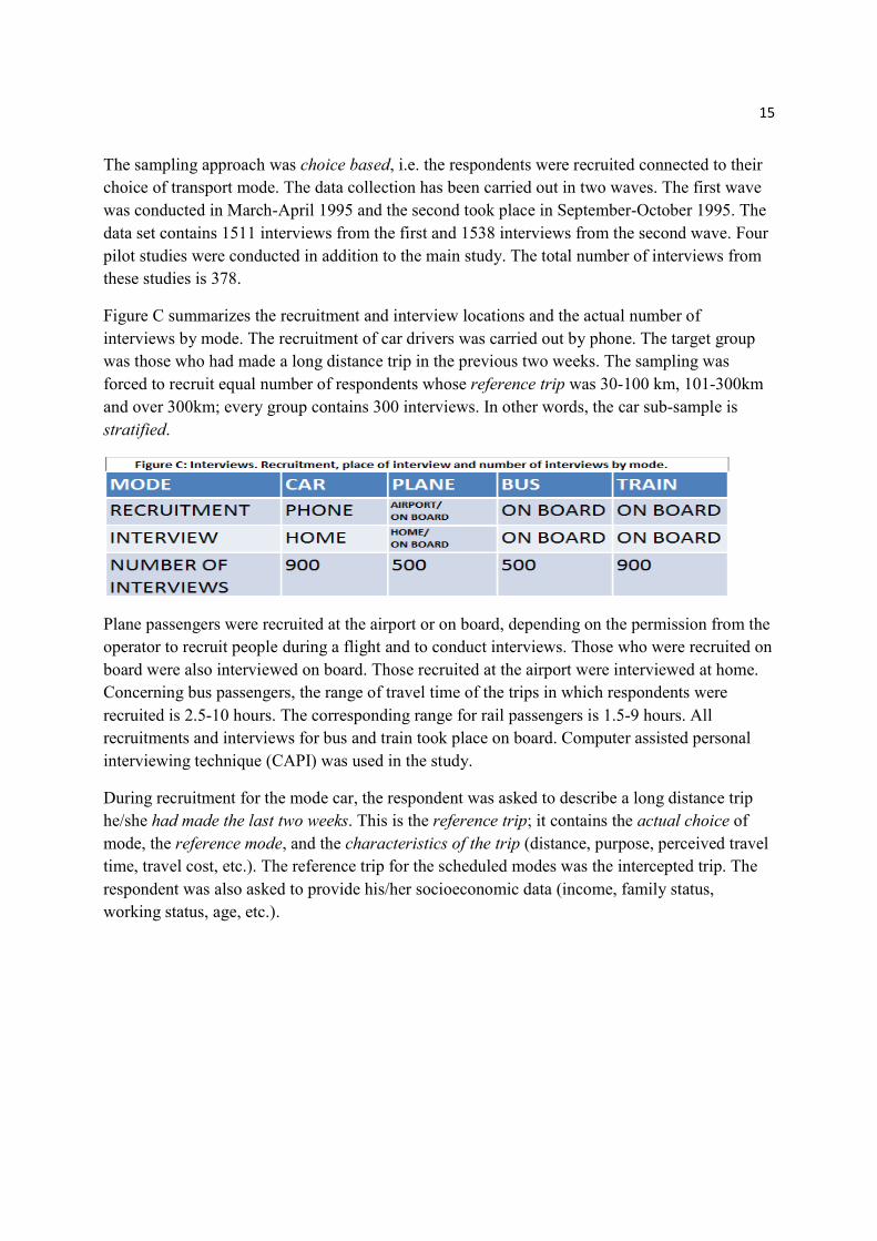
Figure C summarizes the recruitment and interview locations and the actual number of
interviews by mode. The recruitment of car drivers was carried out by phone. The target group
was those who had made a long distance trip in the previous two weeks. The sampling was
forced to recruit equal number of respondents whose reference trip was 30-100 km, 101-300km
and over 300km; every group contains 300 interviews. In other words, the car sub-sample is
stratified.
Plane passengers were recruited at the airport or on board, depending on the permission from the
operator to recruit people during a flight and to conduct interviews. Those who were recruited on
board were also interviewed on board. Those recruited at the airport were interviewed at home.
Concerning bus passengers, the range of travel time of the trips in which respondents were
recruited is 2.5-10 hours. The corresponding range for rail passengers is 1.5-9 hours. All
recruitments and interviews for bus and train took place on board. Computer assisted personal
interviewing technique (CAPI) was used in the study.
During recruitment for the mode car, the respondent was asked to describe a long distance trip
he/she had made the last two weeks. This is the reference trip; it contains the actual choice of
mode, the reference mode, and the characteristics of the trip (distance, purpose, perceived travel
time, travel cost, etc.). The reference trip for the scheduled modes was the intercepted trip. The
respondent was also asked to provide his/her socioeconomic data (income, family status,
working status, age, etc.).

16
2.4 Design of choice experiments
Based on the reference trip and reference mode, a respondent was given a sequence of 11 binary
choice experiments (one SP game). Every binary choice was within-mode, i.e. a choice between a
pair of alternative attribute combinations of the reference mode. Only three attributes were used
in all choice experiments. Figure D summarizes the attributes used for each mode.
Using the values of the attributes in the reference trip as base values, four levels for cost and
travel time and three for frequency of services (scheduled modes) and automatic traffic control
(car) were generated as percentages of the base values. Figures E and F show the percentage
changes of the attributes relative to the base values for car and scheduled modes respectively.

17
The design of the experiment was based on a pre-assumed range of VoT. The VoT range, along
with the percentage change in travel time determines the value of the X, which is the percentage
change in cost. The design used is randomized fractional factorial, i.e. the choice sets do not
include all possible combinations of a full factorial. Dominant choice pairs were not included in
the experiment.
Apart from the reference mode a respondent was asked to choose an alternative transport mode
for the exact same trip. A second SP game with 11 choice experiments was then given to the
respondent. In summary, each interview generated two SP data sets. The first contains the
answers for the choice experiments for the reference mode and the second the responses for the
alternative mode. We return to the use of these data sets later on, in the empirical part.

18
3. Discrete choice and Random Utility models.
3.1. Framework set up for a deterministic choice theory
‘A specific theory of choice is a collection of procedures that defines the following elements’
(Ben-Akiva & Lerman, 1985: pp.32): i) decision maker, ii) choice set, iii) attributes of the
alternatives and iv) a decision rule. Elements i to iii have been determined through the stages of
experimental design; the respondent is exposed to a binary choice situation between two
different combinations of the attributes travel time, travel cost, and a third attributed (frequency
or automatic traffic control) for the same mode. Nevertheless, without a decision rule this
framework set up is incomplete, since it does not describe the internal mechanism used by the
decision maker to analyze information and end up in a unique choice.
The instrument used as decision rule in this study is utility. The accompanying assumption is that
the respondent is attempting to maximize utility through the choice. Thus, in a choice set with
alternatives L and R, the choice of L yields L RU U> and vice versa. The following figure
summarizes framework set up for a deterministic discrete choice theory.
3.2. Random Utility Models
A deterministic framework implies that identical choice situations result in identical decisions
across i) time and ii) individuals. However, in choice experiments, decisions have been observed
to be inconsistent with respect to both of them. This gave rise to the development of Random
Utility Models (RUM), which is the toolkit that economists use to study discrete choice.
The generation of RUM is based on a double assumption. First, preferences remain deterministic
from the decision maker’s point of view, such that if the experiment is replicated for the same
person the decision outcome will be identical (Dagsvik, 2000). Thus, RUM retains a

19
deterministic profile across choice situations, in contrast to other behavioral models (proposed by
psychologists) which allow for an individual’s utility (preferences) to vary according to their
‘psychological state’, such as the Thurstone model.
Second, preferences become random from the econometrician’s point of view, in the sense that
observational deficiencies render the exact form of utility unknown to the analyst. Consequently,
RUM ‘admits’ that if the experiment is replicated for different individuals the decision outcome
does not have to be identical. Therefore, RUM introduces a probabilistic profile across decision
makers. The probability that decision maker n, chooses alternative j in a binary choice situation
between L and R is:
Pr( | , ) Pr( ), , , .nj nij L R U U i j L R i j= > = ≠ (3.1)
We assume that the random utility has an additively separable structure:
nj nj njU V ε= + (3.2)
The first part is a deterministic term which is specified as a function of the observable attributes
and individual characteristics. It is often called the systematic utility. The second term is a
random variable with a hypothetical distribution. It is the part of utility that the researcher does
not observe. See Dagsvik (2000) for a summary of the ‘sources of uncertainty that give rise to
randomness in preferences’. Substituting (3.2) into (3.1) yields:
Pr( ) Pr( ) Pr( )nj ni nj nj ni ni ni nj nj niU U V V V Vε ε ε ε> = + > + = − < − (3.3)
Two assumptions remain for the model to become operational. The first is the specification of
the systematic part of utility. Various specifications are examined throughout the empirical part
of this study. The second assumption concerns the structure of the error terms. It turns that
different assumptions about the error difference lead to different Random Utility Models. From
(3.3) we have:
ɶ ɶ ɶPr( ) ( ) ( )nj niV V
n n nnj ni nj niV V f d F V Vε ε ε
−
−∞< − = = −∫ (3.4)
Thus, any cumulative distribution function can give rise to RUM.

20
3.3. Binary logit
If we assume that ε is identically and independently distributed extreme value type I (iid EV1)
across the two alternatives (L,R) and decision makers, it can be shown that the error difference is
logistically distributed with cumulative distribution function:
ɶɶ
1( )
1 exp( )n
n
F εµε
=+ −
µ > 0, ɶnε−∞ < < ∞ (3.5)
where µ is the scale parameter of the distribution. In order for choice probabilities to be
identifiable, µ has to be fixed to an arbitrary value. A popular choice is µ=1. By combining (3.4)
and (3.5) we get the choice probabilities for the two alternatives:
• exp( )
Pr( | , )exp( ) exp( )
nL
nL nR
VL L R
V V=
+ and
• exp( )
Pr( | , )exp( ) exp( )
nR
nL nR
VR L R
V V=
+ (3.6)
If we further assume linear-in-parameter systematic utilities:
'nL nLV xβ= and 'nR nRV xβ=
the choice probabilities can be written as functions of the parameters. Then (3.6) becomes:
exp( ' )Pr( | , )
exp( ' ) exp( ' )
nL
nL nR
xL L R
x x
ββ β
=+
and exp( ' )
Pr( | , )exp( ' ) exp( ' )
nR
nL nR
xR L R
x x
ββ β
=+
(3.7)
The power of logit as a model lies in its convenient properties. From (3.6) we can check that the
choice probabilities are attained in a closed form expression and sum up to one. It must be
highlighted that this is not the case in models that are reviewed later, such as the probit and
mixed logit since there is no closed form expression for their choice probabilities. This is
intuitively correct and extends directly to choice sets with J alternatives, where Multinomial
Logit (MNL) choice probabilities add up to:
1 1
exp[ ][ ] 1
exp[ ]
J Jni
ni
i inj
j
VP
V= =
= =∑ ∑∑
(3.8)

21
Second, and in contrast to the linear probability model (Maddala, 1983: p.16) from (3.6) it can be
confirmed that the logit choice probabilities, necessarily belong to the interval [0,1]. Third, ‘the
relation of the logit choice probability to the representative utility is sigmoid. If the
representative utility of an alternative is very low compared to the corresponding of other
alternatives, a small increase in the utility of the alternative has little effect on the choice
probability’ (Train, 2002). This has clear policy implications; the logit model suggests that
improvements in the attributes of an alternative (increase in its representative utility) have
greater effect when the binary choice is ambiguous, that is when the choice probability is close to
0.5.
The limitations of logit are summarized in three areas: i) random taste variation ii) panel data and
iii) substitution patterns.
i) Logit can capture taste variation but only within certain limits. Tastes that vary
systematically with respect to observed variables can be incorporated in logit models, unlike
tastes which are correlated with unobserved variables or vary purely randomly. Suppose that
differences in taste are reflected in the coefficients of the attributes of the transport modes, which
we now allow to be individual specific. The impact of a given attribute in the n-th individual for
a given alternative j varies over individuals, so utility is specified as:
n
nj T j C j njU TT Cα β β ε= + + + (3.9)
The systematic utility of a transport alternative is assumed to be a linear function of travel time
(TT) and travel cost (C). We now allow the time coefficient to vary with respect to income of the
individual plus some other factors (frequency of travelling, distance, number of children at home
etc) that are not observed and hence are modeled as random:
n
T n nIβ ϑ η= + (3.10)
Substituting (3.10) in (3.9) yields:
[ ] [ ]nj n n j C j nj n j C j n j njU I TT C I TT C TTα ϑ η β ε α ϑ β η ε= + + + + = + + + + (3.11)
The new composite error is not iid extreme value type I. The covariance of the term for two
alternatives i,j is:
( , ) ( , ) ( , ) ( ) ( ) 0nj ni n j nj n i ni n j n i j i nCov Cov TT TT Cov TT TT TT TT Varε ε η ε η ε η η η= + + = = ≠ (3.12)
and is not zero if the error term η has positive variance. Furthermore, the variance of the error
term is different across alternatives, violating assumption of identically distributed error terms.
By the assumption that µ=1 the variance of the composite term:

22
2
2( ) ( ) ( )6
nj n j nj j nVar Var TT TT Varπ
ε η ε η= + = + (3.13)
depends on the chosen alternative. Logit is therefore a misspecification in the case of random
taste variation. Despite this, the researcher may still choose to use the logit for the sake of
simplicity. But neither does a guarantee exist that logit model approximates the average tastes
nor does it provide information on the distribution of tastes around the average. The alternative
option is to use a probit or a mixed logit model, which can -as we argue in the forthcoming
sections- fully incorporate random taste variation.
ii) The second significant limitation of logit is related to the use of panel data. These are
repeated observations of multiple entities or individuals over time. As in the previous case, logit
remains a good model as long as the error terms are iid. Dynamics in the observed factors
(attributes of the alternative or socioeconomic variables) can be accommodated; the inclusion of
lags does not induce inconsistency in the estimation. On the other hand, dynamics associated
with unobserved factors cannot be handled, since they can carry across individuals and
alternatives.
The inefficiency of logit becomes apparent in this study, which uses a SP data set. This involves
multiple binary choices from the same individual. Consider again travel time (TT) and travel
cost (C) as attributes of the alternative. The utility from alternative j is:
njt T jt C jt njtU TT Cα β β ε= + + + (3.14)
where the subscript t denotes the number of the choice experiment for an arbitrary respondent.
Suppose that the error term contains unobserved socioeconomic variables which do not vary over
choice experiments or alternatives:
n
njt nwε γ δ η= + + (3.15)
where δ is a vector of coefficients, w a vector of socioeconomic variables that are fixed across J
alternatives and T choice experiments for a given respondent n and η is iid in n, j and t. From
(3.15) it can be confirmed that ε is not iid across choice experiments. Thus, logit is a
misspecification in SP multiple choice experiments unless every omitted factor that remains fixed
across choices is fully incorporated in the systematic part of utility. Train (2002) recommends
using a more flexible model such as probit or mixed logit or trying to include the unobserved
factors into representative utility so that the remaining errors are iid over experiments.
iii) The substitution patterns of logit and specifically the Independence of Irrelevant Alternatives
(IIA) property is the most widely discussed limitation in bibliography. A model is said to exhibit
IIA when the relative odds of choosing alternative j over i do not depend on what other
alternatives are available or what the attributes of the other alternatives are.

23
This might not make sense at first, since the data used in the study relate to binary choice sets,
but it is worth having a brief look at this property. The choice probability ratio for binary logit is:
exp[ ] exp[ ] exp[ ] exp[ ]
exp[ ] exp[ ] exp[ ] exp[ ]
nit nit njtnit nit
njt njt nit njt njt
V V VP V
P V V V V
+= =
+ (3.16)
Adding a third alternative in the choice experiments leaves the odds unaffected.
IIA is the direct outcome of the fundamental assumption upon which logit builds, namely that the
error terms are iid (the covariance matrix of the error terms is a diagonal matrix). McFadden
(1974) proves that logit choice probabilities are obtained exclusively from iid type EV1 errors,
even across alternatives. IIA is a rather strong assumption, since the binary choice experiments
of this study are within-mode, i.e. the two alternatives are actually different levels of attributes
(travel time, cost, comfort etc.) for the same transport mode. Thus, there is an extra argument
against the iid assumption, namely that the unobserved factors that influence choice may
correlate stronger between two alternative attribute combinations of the same transport mode that
between two different alternative modes.
3.4. Mixed logit
Mixed logit models can be specified as both random parameter models and error component
models. As it is shown below, the estimation outcome is essentially the same. In the random
parameter specification, we assume once again that the individual n is faced with a choice among
J alternatives (binary choice in this study) in T choice situations. The linear in parameters utility
for choosing alternative j in the choice experiment t is:
'
njt n njt njtU xβ ε= + (3.17)
where x is a vector of attributes of the alternative or socioeconomic characteristics and ε and βn
are unobserved influences which are treated as stochastic. As in the pure logit model, the error
term ε is assumed to be iid EV1 distributed. The parameter coefficients, however, are random
across individuals accounting for random taste variation. We can decompose these coefficients
into their mean b and deviations ηn, or βn = b + ηn. If we substitute back to (3.17) we get:
' [ ]njt njt njt njtU b x η ε= + + (3.18)
where ε is iid EV1 but η can practically be assumed to follow any distribution. The expression in
(3.18) represents an error component model; in this approach the standard deviation of the
random parameter ‘stores’ the heterogeneity as a separate error component. The estimation
outcomes of the two models are identical (Hensher & Greene, 2001).

24
The conditional choice probabilities are logit. This is if ηn was known with certainty for an
individual then the remaining of the error term in (3.18) would be iid EV1 distributed. The
conditional on β choice probability for a sequence of T choices, one for each choice experiment t
is a product of logit formulas:
'
'
exp( )( ) [ ]
exp( )
Tn njt
njt Jt
n njt
j
xP
x
ββ
β=∏
∑ (3.19)
The unconditional probability is the above probability weighted over all values of β:
'
'
exp( )[ ] ( | )
exp( )
Tn njt
njt Jt
n njt
j
xP f d
xβ
ββ β
β= Ω∏∫
∑ (3.20)
Mixed logit choice probabilities are a mixture of a logit choice probability with a mixing
distribution f. “The probabilities do not exhibit IIA and different substitution patterns are
obtained by the appropriate specification of the mixing distribution” (Hensher and Greene,
2001). The probability in (3.20) cannot be calculated in closed form, but can be approximated by
simulation. Mixed logit models are often referred to as hybrid models for this reason; one part of
the resulting choice probability has a closed form and the rest requires simulation.
Frankly speaking, simulation is a sort of imitation of some process. A simulated choice
probability is generated to ‘mimic’ the real choice probability in the following way. A value of β
is drawn from the mixing distribution with parameter vector θ, f(β|θ). For this arbitrary value, the
conditional choice probability is calculated. This process is repeated many times; the number of
necessary draws depends on how fast the simulated choice probability converges to the actual
one, which in turn depends on the variance of the mixing distribution assumed. The simulated
probability is the weighted average of the R conditional probabilities produced by R draws.
1
1( )
Rr
njt njt
r
P LR
β=
= ∑ (3.21)
The parameters of the mixing distribution are then estimated by maximum simulated likelihood
estimation. The simulated log-likelihood function is:
1 1
( ) lnN J
nj nj
n j
SLL d Pθ= =
=∑∑ (3.22)
where dnj equals one when individual n chooses j or zero otherwise, and N is the number of
individuals. Hence, for each individual, R draws are generated and the simulated probabilities for
all alternatives are calculated.

25
When it comes to using mixed logit, a plethora of specification issues arise which constitute the
main challenges in its application. The first is to select which of the parameter coefficients will
be random and which are going to be kept fixed. A second one to decide in favor or against
recommended mixing distributions. The choice of the mixing distribution is a central issue.
‘Actually, various pieces of research have demonstrated that an inappropriate choice of the
distribution may lead to serious bias in model forecast and in the estimated mean of random
parameters’ (Fosgerau & Bierlaire, 2007). Panel data, often in the form of stated choices also
pose a challenge since the researcher has to somehow account for the fact that several choices
come from the same individual. These problems will be further discussed from an empirical
point of view as we proceed to the specification of our econometric model.
3.5. Binary probit
‘One logical assumption is to view the disturbances as the sum of a large number of unobserved
but independent components. ‘By central limit theorem the distribution of disturbances would
tend to be normal’(Ben-Akiva & Lerman, 1985). The binary probit model is derived from the
assumption that the disturbances of the two alternatives (L,R) are both normal with zero mean,
variances 2 2,L Rσ σ and covariance LRσ . The distribution of the error difference is
ɶ 2 2(0, 2 )L R LRNε σ σ σ+ −∼ (3.23)
is also normal. Then (3.4) becomes:
ɶ ɶ ɶ1 1Pr( ) exp[ ( / )] ( )
22
nj niV Vnj ni
n nnj ni
V VV V dε ε σ ε
σσ π
−
−∞
−< − = − = Φ∫ (3.24)
where 1/σ is the scale of utility. By allowing error terms to follow any pattern of correlation,
probit can accommodate the main drawbacks of logit. It can be shown that probit choice
probabilities do not exhibit the IIA property (since disturbances can follow any pattern of
correlation). Probit can also handle random taste variation, as long as any random coefficient
follows a normal distribution with mean b and standard deviation σ.
Despite these desirable properties, the choice probability does not have a closed form expression
and can only be approximated by simulation. This fact rendered probit models less attractive
than mixed logit, in which only one part of the choice probability has to be approximated by
simulation. Probit models will not be used in this study.

26
4. VTTS estimations
4.1. Estimation of VTTS with Logit specification
We set as point of departure the simplest form of MNL model in which the utility of the chosen
alternative is a linear function of the required travel time, cost and F. F, the third attribute, is
frequency for the scheduled modes and ‘automatic traffic control’ for car. The respondent faces a
sequence of within-mode binary choice situations between two alternatives (both alternatives
refer to the same transport mode, i.e. the reference mode, they are considered as different
alternatives, however, since the levels of attributes are different). In each choice situation, we
denote them as left (L) and right (R). The choice of L and R is arbitrary. For instance numbers (1 and 2) could have been used instead. We specify the systematic utility as linear in the attributes
travel time (TT), cost (C) and frequency (or automatic traffic control) (F).
cosL time L t L freq LV TT C Fα β β β= + + +
RV = costime R t R freq RTT C Fβ β β+ + (Model 1) (4.1)
The coefficients of the attributes are specified to be generic, i.e. not alternative specific, since they all refer to the same transport mode. We also introduce an alternative specific constant for
the left alternative. This constant is interpreted as the average effect of the omitted factors on the
utility of the left alternative relative to the right (Train, 2002). Since both L and R refer to the
same transport mode, this term is not expected be significantly different than zero. It should be
included, however, to check for order effects and lexicographic answers. Significance of this
term would be a sign that some of the respondents answered lexicographically, or that there is
something intrinsic in the design of the questionnaire that favors one of the alternatives.

27
Despite this, the structure of the randomized fractional factorial does not suggest any reason that
could make an alternative more favorable just because it appears on the left or right side of the
screen. The same structure also rules out lexicographic answers, i.e. answers that reflect
decisions taken with respect to one attribute (for example, the respondent always chooses the
cheapest alternative), to be the reason for favoring an alternative because of the order of appearance on the screen. It is however possible that some respondents systematically choose an
alternative because of the order of their appearance on the screen. Since with roman alphabets
people read from left to right, it is likely that some respondents would select the first alternative
they see on the screen, the left one.
We estimate the parameters of Model 1 with BIOGEME 1.5 (Bierlaire, 2003) for the four strata;
car drivers and plane, bus and train passengers (one sub-model for each group). Both coefficients
are specified to be constant in the population. Therefore we get a constant estimate of value of
travel time (VTT) for each stratum. The estimation results are presented in Table 1. The
estimates of VTT from every sub-model are expressed in 1995 Norwegian Kroner (NOK) per
minute of travel time. Therefore, they must be multiplied by 60 to give an estimate of per hour VTT. The estimates of per hour VTT are approximately: 88 NOK/hour for car, 179 NOK/hour
for plane, 35 NOK/hour for bus and 48 NOK/hour for train.
The estimates of βtime and βcost are significantly different than zero in all sub-models. The robust
t-tests are relatively high to guarantee zero p-values. Thus, the null hypothesis of insignificant
time or cost coefficients is rejected at every convenient level of significance. The robust standard
error and consequently the t-test for the VTTS have been computed from a second-order Taylor
series approximation. Again, the high t-values in the four sub-models imply that the hypothesis
of insignificant VTT can be rejected at any level of significance.

28
The flexible third attribute is not significant in all sub-models. In the car sub-model, it refers to
the number of photo-box speed detectors in a given stretch of the road (see Chapter 2). The
estimate is statistically significant and negative, implying that drivers perceive speed detectors as
a hurdle on the desired speed or perhaps a worry about exceeding the speed limit and getting a
fine. For the rest of the modes, the attribute refers to frequency and is associated with the time interval between two departures. The estimate for plane passengers is negative and highly
significant –the longer the time intervals between flight departures the lower is the utility with
plane. The frequency coefficient estimates for bus and the train sub-models are insignificant.
The insignificance of the alternative specific constant in car, plane and train sub-models is not
surprising; the omitted factors that generate (dis)utility are identical for the alternatives L and R,
since the two alternatives refer to the same transport mode. Thus the average impact of omitted
factors should not be different for the two choices. In the bus case, however, the null hypothesis
for insignificant within mode constant is rejected at levels of significance smaller than 0.02, as
the p-value suggests. In this case, p-value is the probability of estimating a bus constant at least
as different than zero as 0.0825, assuming that this constant is in fact zero (Stock & Watson, 2003: pg. 113).
A re-estimation of the sub model for bus without constant sheds light in the paradox; the
coefficient estimates, and consequently the estimate VTT, are almost identical. Table 2 presents
these results.
We now turn to the discussion of the summary statistics that accompany the estimation process
and are placed in table 3.
For each of the sub-models, the null log-likelihood, (0)L , is the value that the log-likelihood
function attains when all parameters are set to zero. “In binary choice models it is the log
likelihood of the most ‘naive’ model, that is, one in which the choice probabilities are ½ for each
of the two alternatives” (Ben-Akiva & Lerman, 1985). The initial log-likelihood, 0L( )β , shows
the value of the log likelihood function before any maximization algorithm is applied. It depends
on the initial assigned parameter values by the researcher. We fixed initial values of betas to

29
zero. The final log-likelihood, ( )mleL β , is the value that the log likelihood attains when its vector
of parameters is replaced by the ML vector of estimates, mleβ .
The log-likelihood ratio test (LR test) is used the same way F-test is used in linear regression
models, i.e. to test for the hypothesis that the ‘real’ model is significantly different than the
‘naïve’, in which all parameters equal zero. The associated test statistic has unknown small-
sample distribution, but is distributed asymptotically as a chi-square (χ2) with degrees of freedom
equal to the number of restrictions being tested (Kennedy, 2003). Knowing that the null
distribution is χ2 makes possible for the construction of rejection region for any level of
significance. In the present case the test rejects the null hypothesis if:
LR-test = 2
42[ (0) ( )] ( )mleL L β χ α− − > (4.2)
since four parameters are restricted to be zero under the null hypothesis. The LR tests of all sub-models are high enough to reject the null hypothesis at any level of significance. Ben-Akiva and
Lerman (1985:pg165) argue that LR test is not very useful since it almost always rejects the null
hypothesis, even at a very low level of significance.
The ρ2 and the adjusted- 2ρ , or McFadden’s likelihood ratio index, are informal indexes for the
goodness of fit which are analogous to R2 and the adjusted-R
2 in linear regression and -in a
nutshell- measure how much of the initial log-likelihood is explained by the model (Ben-Akiva
and Lerman, 1985). The formulas for the two indexes are:
2 ( )
1 [ ](0)
mleL
L
βρ = − (4.3) and
adjusted-
2 ( )1 [ ]
(0)
mleL K
L
βρ
−= − . (4.4)
The very high values of the final likelihood relative to the number of parameters K=4 explain
why the differences between these indexes are tiny. The adjusted likelihood ratio is between 0.11
and 0.144 for all transport modes apart from bus, for which ρ2 is much lower, 0.06.
Greene
(2003) points out that this measure has an intuitive appeal in the sense that it is bounded between zero and one and that it increases as the fit of the model improves but -unlike R2 in linear
regression- its values have no natural interpretation.
These measures will be used in comparison with their respective from alternative specifications
presented later on. The low values, however, are a warning sign that the model specification can
be improved, by adding more explanatory variables and by altering the strict assumptions of
logit.

30
4.2. Do we really need Mixed Logit?
As a pure logit, Model 1 will present all the significant drawbacks discussed in the Chapter 3.
The specification proposed in Model 1, implies a uniform VTT for each stratum. In fact, by
assuming a degenerate distribution for the coefficients of time and price, we automatically ignore
the fact that VTT may significantly vary across members of the same stratum. In other words, we
neglect heterogeneity. A random coefficient model, on the other hand, allows for a within-mode
non-degenerate distribution of VTT (Chapter 3). We are interested in estimating the parameters
that describe this distribution, and subsequently its moments.
Before specifying a random coefficient model (mixed logit), it might be a good idea to perform a Likelihood Ratio (LR) test to check for unobserved heterogeneity in the stratified samples. In
other words we need to check the hypothesis that the coefficients are fixed against the
alternative, that they are random across individuals. The following LR test is proposed in
McFadden and Train (2000). A Lagrange Multiplier variant of this test is also available in
Bolduc (2008).
Consider the choice from the set C = L,R and the vectors of attributes for the two alternatives
XL = ( TL, CL, FL ) and XR = ( TR, CR, FR ). These attributes are the same as those used in Model
1 of section 4.1. From a random sample of N individuals we estimate the parameters for these
attributes with logit. These are simply the ML estimates of the coefficients of Model 1.
The next step is to calculate the logit choice probabilities for the two alternatives:
( , ) exp[ ] exp[ ] exp[ ]L rfL rfL rfRLP x V V Vβ = +
and
( , ) exp[ ] exp[ ] exp[ ]R rfR rfL rfRRP x V V Vβ = + (4.5)
then we calculate the auxiliary variables for cost and time:
*( , ) ( , ) ( , )
n
j L Rj j L L R R
j C
C C P x C P x C P xβ β β∈
= = +∑ and
*( , ) ( , ) ( , )
n
j L Rj j L L R R
j C
T T P x T P x T P xβ β β∈
= = +∑ (4.6)
And use them to construct the four artificial variables:
* 20.5[ ]CL LZ C C= − , * 20.5[ ]CR RZ C C= − , * 20.5[ ]TL LZ T T= − and * 20.5[ ]TR RZ T T= − (4.7)
For each stratum, we add the artificial variables to Model 1 and estimate the following model:
31
cos cosrfL time L t L fq L t CL time TLV TT C F Z Zα β β β γ γ= + + + + + (Model 1’) (4.8)
rfRV = cos costime R t R fq R t CR time TRTT C F Z Zβ β β γ γ+ + + +
We then use a likelihood ratio test for the hypothesis that the artificial variables Z should be
omitted. The intuition behind the generation and inclusion of these artificial variables is that they
are designed to ‘catch’ some sort of variance in the coefficients across individuals. For example,
for a randomly selected individual with probabilities to select the left and right alternative
( , )L LP x β and ( , )R R
P x β respectively, the auxiliary variables T* and C
* represent the expected
travel cost and travel time. The variable * 20.5[ ]LT T− then represents a type of taste variation
around the mean.
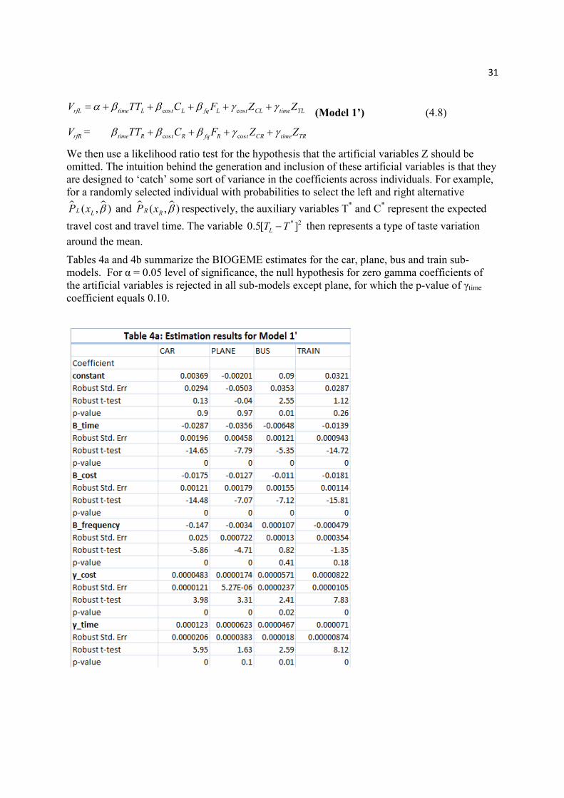
Tables 4a and 4b summarize the BIOGEME estimates for the car, plane, bus and train sub-
models. For α = 0.05 level of significance, the null hypothesis for zero gamma coefficients of
the artificial variables is rejected in all sub-models except plane, for which the p-value of γtime
coefficient equals 0.10.

32
We now perform a Likelihood Ratio test for the null hypothesis that Model 1 is the real model,
that is, the coefficients of both artificial variables are zero, against the alternative which suggests
that Model 2 with artificial variables is superior.
H0: γcost = γtime = 0
The Likelihood Ratio is:
0
1
( )
( )
mleH
mleH
lik
lik
β
βΛ =
(4.9)
And the test statistic: 0 1 0 1
0 12log 2[log ( ) log ( )] 2[ ( ) ( )]
H H H H
mle mle mle mleH Hlik lik L Lβ β β β− Λ = − − = − − is
asymptotically χ2 distributed with 2 degrees of freedom. The critical value for α = 0.01 is 9.21.
The test rejects the null hypothesis for all sub-models as shown in the test summary below.
This Likelihood Ratio test is asymptotically equivalent to a Lagrange Multiplier test for the
hypothesis of no mixing against the alternative of mixed logit with randomized time and cost
coefficients as proved by McFadden and Train (2000).
The above test gives ‘the green light’ to the researcher to move further and specify a mixed logit
model with random time and cost coefficients. It does not, however, suggest which mixing
distribution should be used. Neither does it imply an optimal modeling option for the interests of
the researcher. Actually, the idea of a jointly mixed logit (when both cost and time coefficients
are random) is associated with a higher computational cost of VTT. These issues are discussed in
the next sections, in which we take the first step to mixed logit.

33
4.3. Which parameters should be random?
The Likelihood Ratio test by McFadden and Train suggests that both time and cost partworths
(coefficients of utility function) should be modeled as random across individuals. Modeling both
of them as random would be the most realistic case. Nevertheless, there are serious reasons to
model only one of them –the time coefficient- as probabilistic and keep the other one-the cost coefficient- fixed.
Assigning a joint distribution to bcost and btime involves accommodating the correlation between
them, which may not be an easy task. Second, the method of parametric estimation in mixed
logit models, Maximum Simulated Likelihood, involves draws from the bivariate distribution
cos( , )t timef β β in order to approximate the mixed logit choice probability:
cos
cos cos cos( ) ( | , ) ( , )
t time
t time t time time tP i i f d dβ β
β β β β β β= Λ∫ ∫ .
In many cases this might be an additional complication, depending on the assumptions about the
joint pdf (probability distribution function) of the partworths.
Also, the distribution of VTT, that is the distribution of the ratio of timeβ on cos tβ , might be
unknown. Since the interest of this study is concentrated on VTT, the assumption of non-random
cos tβ facilitates the modeling of VTT distribution. Consider the case where timeβ follows a normal
distribution with mean µ and standard deviation σ, [ ( , )t ttime N β ββ µ σ∼ ], and cos tβ is constant.
Then, cos ( , )t t
time t
c c
VTT Nβ βµ σ
β ββ β
= ∼ . It is therefore possible to estimate the mean and the
standard deviation of VTT by estimating the cost coefficient and the mean and the standard
deviation of the random time coefficient. Thus, for the remaining it is going to be assumed that
only timeβ is random. Its probability distribution function is called the mixing distribution. The
choice of this density function is the topic of the next section.
4.4. Which ‘mixing distribution’ to use?
Distributions are essentially arbitrary approximations to the real behavioral profile. ‘We select
specific distributions because we have a sense that the empirical truth is somewhere in their
domain’ (Hensher & Greene,2001: pp.146). This study experiments on the Normal, Log-Normal
and Johnson’s SB distribution as mixing distributions.
The most commonly used distribution in mixed logit models is the Normal, mainly because of its
low computational cost. On the other hand, the fact that the domain of the Normal density function is the entire real line means that some of the mass of the VTTS will inevitably fall on
the negative side. The implicit assumption of the model is that negative values of travel time
savings (or, equally, positive values of travel time) exist in the population with some probability
that depends on the estimated parameters of the normal distribution.
34
If data allows for such a possibility, then Normal is able to reveal this effect, and is in fact a good
mixing distribution for time coefficients. ‘The issue with the Normal distribution is thus the
problem of deciding whether a non-zero probability of a positive coefficient is revealed by data
or is simply an artifact of the symmetrical nature of the distribution’ (Hess et al., 2005). The data
used in this study do not allow for negative VTTS; the unbounded nature of the normal distribution just ‘forces’ the model to produce negative VTTS (positive VTT). Model 2
introduced in section 4.5 uses Normal as a mixing distribution. An example with Normal mixing
distribution for the time coefficients can be found in Algers et al. (1998).
Truncated mixing distributions is a possibility that has been discussed in the literature by
Hensher and Greene (2003), Train and Sonnier (2004) and Train (2002). By truncating the
Normal distribution of time coefficient at zero, the researcher can constrain VTTS to take only
positive values. Despite being a promising development for the future, Truncated Normal is
excluded from this study since BIOGEME 1.5, has not incorporated it yet.
Nevertheless, the same software allows for MSL estimation with other bounded mixing
distributions, as long as they are transformations of Normal. We use a semi-bounded distribution
with fixed lower bound at zero, namely the Lognormal (Model 3) and a two-side bounded with
flexible upper and lower bound, namely the Johnson SB (Model 4). The former has been used in
the literature to model random coefficients with unambiguous signs, such as price. Train and
Sonnier (2004) compare a model with a joint Normal mixing distribution for its random
coefficients to a counterpart in which partworths follow the Lognormal, in the context of a
vehicle choice study. The model with Lognormal mixing distribution showed a substantially
higher log-likelihood than its Normal counterpart.
The main disadvantage of Lognormal distribution is its thick tail. The behavioral implication of
the thick tail is the existence of obscurely high WTP for time savings for some share of the
population. As in the case of Normal distribution, extremely high WTP may, or may not be
supported by data. The justification of Lognormal as a good mixing distribution depends on
whether the sample exhibits the above property. Model 3 in section 4.6 uses Log-Normal as
mixing distribution.
The mixing distribution used in models 4a and 4b is the Johnson SB. Its main advantage lies in its
flexibility. Either both bounds can be fixed ex ante and the mean and standard deviation can be estimated by MSL (section 4.9) or one of the bounds can be fixed ex ante and the rest of the
three parameters can be estimated by MSL (section 4.8). Setting both bounds as random
parameters for estimation involves simulation with a sort of quasi-random draws, Gibbs
sampling (Train, 2002: pg.215). This goes beyond the scope of this study. The distribution is
very flexible and can take lots of shapes, depending on its range (Johnson1994: pg.37).
The use of Johnson SB as mixing distribution is relatively recent and encouraged in literature.
Train and Sonnier (2004) fix the lower bound at zero and the upper bound at a value ‘high
enough to accommodate nearly all the cumulative distribution function’ of Log-normal. The SB
provided a ‘plateau’ shape distribution that Log-normal cannot produce and the log-likelihood
increased significantly. Hess et al. (2005) used the SB and compared it to models with Normal and Log-normal mixing distribution. Unfortunately, recovering the SB moments from the
moments of a Normal distribution is not an easy task. Methods for the calculation of the SB
moments are presented in Johnson et al. (1994, pg. 35). Another solution would be simulation; to
use the normal invert cdf, in order to draw observations from the SB distribution and approximate

35
its moments. This is how VTTS estimates are obtained for models 4a and 4b in sections 4.8 and
4.9 respectively.
Another possibility is the Triangular distribution. It is rarely used in hybrid contexts, mainly
because of its linear tails. However, it theoretically overcomes the drawbacks of Normal and
Log-Normal; its bounds prevent negative VTTS or extremely high WTP. Nevertheless, neither
Hess et al. (2005) nor Train and Sonnier (2004) incorporate Triangular in their models. An
empirical comparison between mixing distributions containing Triangular can be found in
Hensher and Greene (2003).
4.5. Normally distributed time coefficient
We now specify a model with a random time coefficient that is assumed to follow the normal
distribution.
cos
n
nL time L t L f LV TT C Fα β β β= + + +
nRV = cos
n
time R t R f RTT C Fβ β β+ +
(Model 2) (4.10)
where ( , )n
time Nβ µ σ∼ and βcost, βf are generic and fixed in the population. Like the models of the
previous sections, Model 2 is applied to four strata; choices are between L and R in a within-
mode context. MSL estimation has been carried out sequentially in four steps; initially with 100
pseudo-random draws, then by using these results as starting values an estimation with 250
draws followed. The process was repeated for 500 draws and the results were used as starting
values for the final estimation with 1000 draws. The improvements in terms of fit and final log-

36
likelihood in comparison with Model 1 are remarkable. Table 6a summarizes the estimation
results for Model 2.
All alternative specific constants are highly insignificant (p-values bigger than 0.1) except for the
bus sub-model in which it is insignificant at α = 0.01. Frequency is also insignificant for the
same mode. The rest of the coefficients are significantly different than zero. These facts are
generally in accordance with Model 1 (pure logit). The 95% upper and lower percentile limits are
the values of βtime for which the associated cdf of the fitted distribution equals 0.95 and 0.05
respectively.
Table 6b presents the estimates of the parameters of the VTTS distribution, which are functions
of the estimates of costβ , µ and σ . The mean VTTS estimates from Model 2 are higher than
the uniform VTTS estimates of Model 1. This contradicts the results of Algers et al. (1998)
where mean VTTS estimates in a random time coefficient model with fixed cost coefficient for
pooled (WTP and WTA samples) data are lower than those from a classic logit. On the other
hand, Hess et al. (2005) estimated VTTS to be much higher with a mixed logit model than with
pure logit.

37
Based on the fitted VTTS distribution, estimates of the 95% upper quantile limit are presented in
Table 6b. These estimates are the implied price limits that ‘cover’ 95% of the population’s WTP
for time savings in NOK per minute and per hour. The model implies for instance, that 95% of
the car drivers (sub-model 3a) are willing to pay up to 312.73 NOK to reduce driving time by one hour. The other side of the same coin is that 5% of the car drivers are willing to pay more
than 312.73 NOK to save one hour of driving time.
The probability that VTTS is negative is neither supported by economic theory, nor is built in the
data, since the design of the questionnaire does not allow for such a possibility. Despite this, the
Normal distribution as a model forces VVTS to take both positive and negative values. The value
of the fitted Normal cumulative distribution function at zero equals the estimated probability of
negative VTTS. Therefore, the sub-models’ estimates (wrongly) imply that 14.01% of car
drivers, 12.71% of plane passengers, 29.81% of bus passengers and 19.77% of train passengers
are willing to pay for a longer trip time.
To have a visual image of these aspects, the VTTS distributions for the four sub-models have
been simulated with 1000000 draws each. The images are given in Figure J. The red part of the
mass represents the simulated probability of negative VTTS, while the dark shadow on the right
tail is the simulated 95% upper quantile limit.

38
This wrong behavioral implication is the main disadvantage of the normal distribution. The next
model introduces the Lognormal as mixing distribution. As a model, Lognormal solves the above
problem by ‘forcing’ VTTS to be non-negative. On the other hand, one other peculiarity arises,
associated with the unbounded thick tail of the distribution, which may imply extremely high
VTTS for a significant share of the population.

39
4.6. Log-Normally distributed time coefficient
A model in which cos( ln , )tVTTS LN µ β σ−∼ can be specified from:
cos
n
nL time L t L freq LV TT C Fα ζ β β= − + + (Model 3)
nRV = cos
n
time R t R freq RTT C Fζ β β− + + (4.11)
where ζ is an exponentiated pseudo-random draw from a Normal distribution with parameters µ
and σ, such that n
n eβζ = . All sub-models of Model 3 were estimated sequentially in two steps.
First, MSL estimation was carried out for 100 pseudo-random draws and the estimates were used
as initial values in the second step, where MSL estimation was repeated for 1000 Lognormal
draws. Table 7a shows the estimation results for Model 3.
As in Model 2, alternative specific constants in all sub-models are not different than zero at all
convenient levels of significance apart from the alternative specific constant in the bus sub-
model, which is not zero at α = 0.01. The estimates of µ and σ are highly significant. The mean
and the standard deviation of the associated Lognormal distribution are functions of these parameters given by Train (2002: pp. 209) and Johnson et al. (1994). These are:
• 2( ) exp[ ( 2)]E β βζ µ σ= + and
• 2 2( ) exp(2 )[exp( ) 1]Sd ζ µ σ σ= + − . (4.12)

40
All cost coefficients are statistically significant and have the expected (negative) sign. Like in
previous models, the frequency coefficient is insignificant at α = 0.05 for bus and at α = 0.01 for
train. Table 7b presents the estimation results concerning VTTS, and the summary statistics.
The mean and standard error VTTS are calculated using (4.12). The estimated VTTS for car and
plane in this model are higher compared to the estimates from the model with Normal mixing
distribution. This is in accordance with the study of Hess et al. (2005) in which the mean
Lognormal VTTS is higher than the Normal; and also with Hensher and Greene (2003) in which
the mean Lognormal VTTS estimates are more than three times higher than the mean VTTS
estimated from an mixed logit with Normal mixing distribution. On the other hand, VTTS for
bus passengers is slightly lower than its respective from Model 2.
The most remarkable result is the unexpectedly high VTTS estimate for train passengers, which
is almost eight times the VTTS estimate from the model with Normal mixing distribution. This
may look odd at first sight, but can be explained by the high standard deviation estimate; the
model estimates that µ = - 4.83 and σ = 2.51. Both the mean and the standard deviation of

41
lognormal density are exponentially increasing in µ and σ. Also, by definition the mean of
Lognormal is a function of both µ and σ. By moment transformation, a Log-normally distributed
time coefficient has a mean of 9.758 and a standard deviation of 227.522 (Table 7b). High value
of σ produces a very long, thick right tail. This suggests that quite often an extraordinarily high
value will be drawn from this density, pushing the mean to higher values. The implication is that Lognormal is not a good model when observations are quite diverse, as in the train sub-model.
The 95% quantile limit is the invert VTTS cumulative distribution function evaluated at 0.95.
This is the WTP for travel time savings that ‘covers’ 95% of the population. It also implies that
there is still a 5% share of drivers or passengers whose willingness to pay is higher than this
value. This value is 572 NOK/h for car drivers and 1049 NOK/h, 126 NOK/h, 1558 NOK/h for
plane, bus and train passengers respectively. Again, the peculiarity of the estimate for train lies in
the high underlying σ.
The moments of the Lognormal distribution of the time coefficient can also be approximated by
simulation. Using the estimates of µ and σ, we draw 20000 observations from N(µ,σ) and
exponentiate them. The transformed observations follow the Lognormal distribution and their
average is the simulated mean while their standard deviation is the simulated standard error.
From Table 7b we see that the ‘simulated mean VTTS’ for all sub-models are quite close to the
approximate means of the first line. The close relation also holds for the simulated and estimated
standard errors, except for the train case, in which the simulated standard error is significantly
smaller, approximately 85.3, against 227.5 which is the estimate we obtain by transformation.
The simulated 95% upper quantile limits were obtained by drawing 20000 observations from a
Lognormal with MSLµ and MSLσ , rank them, and observing the cut-off value of the 19000-th
observation. These values are generally consistent with the values obtained by the Lognormal
cdf.
The final log-likelihoods are lower than those from the Normal mixing distribution model
(Model 2) for all sub-models, but still higher than those from logit model (Model 1). The
likelihood ratio test is high enough to reject the null hypothesis under which all coefficients are
zero. The likelihood ratio index (adjusted ρ2) is also higher than the logit model’s but lower than
the mixed logit model’s with Normal mixing distribution, for all sub-models.
4.7. A bootstrap experiment
An insight into the inherent variability of the maximum simulated likelihood estimates of VTTS
can be given with bootstrap, which is a recent development in statistics used to approximate the
unknown sampling distribution of the estimated parameters of a distribution. We apply it to
compare the estimated moments (mean and standard deviation) in the sub-models for car and
train under Lognormal mixing distribution of time coefficients. For these two modes 1000
samples, with 1000 observations each, drawn from a Lognormal distribution with parameters
MSLµ = -4.83, MSLσ = 2.51 for train and MSLµ = -3.57, MSLσ = 1.16 for car are generated (the true
µ and σ are unknown). In other words, we repeat the simulation process 1000 times. The aim is
to check the stability of the estimates across the samples.

42
For each 1000-sample the empirical lognormal mean and standard deviation is estimated (denote
them by *
iε and *
iω respectively for the i-th 1000-sample), such that a set of 1000 vectors
( *
iε , *
iω ) is obtained. The average values ε and ω , which are then given by 1000
*
1
1
1000iε ε= ∑ and
1000*
1
1
1000iω ω= ∑ will be biased towards the mean and the standard deviation of a lognormal
density with parameters MSLµ and MSLσ , that is towards 9.758 and 227.522 for train and 2.773
and 4.673 for car (Table 7b). The standard errors however, which are given by
*
1000*
1
1( )
1000i
sε
ε ε= −∑ and *
1000*
1
1( )
1000i
sω
ω ω= −∑ are concise quantifications of the amount
of variability of the estimates of the lognormal mean and standard deviation. Bootstrap is
described in Rice (2003).
The results are given in Table 8. In the case of car, the bootstrap VTTS per minute and the
bootstrap standard deviation of VTTS per minute are close to the estimates of Table 7b. The
standard error of the bootstrap mean shows the variability of the estimate across samples of 1000
observations. Its small value renders the simulated mean VTTS in table 7b a reliable estimate.
On the other hand, the variability of the bootstrap standard error of VTTS in car is not negligible,
so the observer should be tentative when utilizing the estimates of standard deviation.
In the case of train, the enormous variability of both the bootstrap mean and standard error,
suggests that we cannot rely on the estimates of Table 7b when assessing VTTS for train
passengers. This may in turn imply that Lognormal is not a good model for VTTS when data are
not informative as in sub-model 3d. Figure L shows the two histograms that display the
difference in the variability of the means for car and train.

43
4.8 Johnson SB distributed time coefficient
We now turn to a relatively new and very interesting type of mixing distribution, namely the
Johnson SB distribution (Johnson et al., 1994). If the time coefficient is normally distributed, the
transformation:
exp( )( )
[1 exp( )]
n timetime
time
βξ λ ν λ
β= + −
+ (4.13)
is said to follow the Johnson SB distribution where λ is the lower cut-off point and (ν-λ) the
range. Since βtime is normally distributed, exp( )
[1 exp( )]
time
time
ββ+
belongs to the open interval (0,1). It

44
follows that n
timeξ defined in (4.13) belongs to the interval (λ,ν). It is a requirement that λ is non-
negative. The specification for the within mode choice Model 4 is:
cos
n
nL time L t L freq LV TT C Fα ξ β β= − + +
nRV = cos
n
time R t R freq RTT C Fξ β β− + + (Model 4) (4.14)
The estimation was carried out at once with 500 draws, without prior values, except for the car
sub-model, in which initial values from an estimation process with 200 draws were used. The
lower bound of the time coefficient, and hence the minimum WTP to save time, was fixed to zero.
The upper bound was set to be a free parameter and then estimated for the four transport modes.
The reader must bear in mind that the use of Johnson SB in this study is purely experimental, mainly because of a relative scarcity of other applications and examples in VTTS bibliography.
Thus, despite sensible, the results of this section must be taken into account tentatively. Table 9a
presents the results of the estimation.

45
The µ and σ coefficients appear to be not significant at α = 0.1 for the car, plane and bus sub-
models. On the other hand, the same coefficients are significant at α = 0.05 in the model for
train. The cost coefficients are significant in all modes, and have the expected negative sign. As
in previous model estimations, frequency appears to be insignificant in the bus sub-model and
not significant at α = 0.01 in the rail sub-model. All alternative specific constants are insignificant, except for bus in which the constant remains significant at α = 0.05.
The new estimate is the upper bound of the time coefficient distribution. This value divided by
the negative of the cost coefficient, gives the maximum WTP for time savings in a specific
transport mode. The estimates of the upper bound are significant at α = 0.05, apart from the
plane sub-model.
The fit of the model is lower that the fit provided by the model with Normal mixing distribution,
but higher than its Lognormal counterpart; the adjusted ρ2 index of Model 4 is higher compared
to Model 3, for all sub-models. The same result holds, when comparing the likelihood ratio tests
of the Models 2-4.
The moments of the Johnson SB distribution are not a closed form expression of the parameters µ
and σ, so recovering them by the estimates is not an easy task. Nevertheless, the mean and the
standard deviation of the time coefficient can be approximated by simulation. For each sub-
model, 20000 observations were drawn from a Normal distribution with the estimates for µ and σ
as parameters. These observations were transformed into 20000 Johnson SB observations, by
using the estimated upper bound in each mode. The average of this 20000-sample is the simulated mean and its standard deviation is the simulated standard deviation.
Table 9b presents the simulated estimates. For car, bus and train sub-models the simulated VTTS
estimates are higher than the corresponding from logit model but lower than the same estimates
from the other mixed logit models. For the rail sub-model, the VTTS estimate exceeds its
estimated value from the model with Normal mixing distribution, but is still way smaller than the
unrealistic estimate from the model with Lognormal mixing distribution. The upper bound VTTS
is the estimated maximum willingness-to-pay for time savings in a given mode.
A visual image of the Johnson SB distribution can be given by the histogram of the simulated VTTS distribution for the four modes, as shown in Figure N. All simulations have been
performed with 1000000 draws. The shape of the Johnson SB distribution depends on its range.
The simulated VTTS distributions for car, bus and rail sub-models are sharply U-shaped.
Johnson et al. (1994: pg.37) highlight the possibility of U-shape.

46
Nevertheless, the interpretation of a U-shape VTTS distribution is counterintuitive, since it
implies that a big share of the drivers (or passengers) is willing to pay almost nothing in order to
save time. At the same time, a significant share of the market is willing to pay the upper bound
limit price, but no more than that. The rest of the population is almost uniformly distributed in
terms of WTP, with very small shares. Thus, the transition from low WTP to high WTP is not smooth in terms of market shares. For the plane sub-model the simulated distribution has a
different shape, to which an exponential or Gamma curve might fit better. The share is
monotonically decreasing in WTP. The convex shape suggests that the rate of decrease is falling
as WTP gets higher.
4.9 Johnson SB with fixed upper bound
We now perform the following experiment. We fix the upper bound to a value that, with the
existing estimates from the free upper bound model, accommodates 99.9% of WTP in the model
with Normal mixing distribution. These are approximately 478.72 NOK for car, 900.06 NOK for
plane, 305.74 NOK for bus and 350.63 NOK for train.

47
The sub-models are then re-estimated with their upper bounds fixed. Table 9c presents the results
and Figure O the corresponding simulated VTTS distributions. In contrast to Model 4, all µ and
σ estimates from Model 4’ are significant, with zero p-values.
The simulated histograms are generated with 100000 draws. What is remarkable is the intuitive
improvement in the shape of the VTTS distribution in the population for the modes car, plane
and bus. The implied behavioral profile of the distributions in Figure O is undoubtedly more
compatible with reality, assuming a monotonic decrease of density in VTTS, after the last has
attained its peak. The implication is that a big share of the market is willing to pay small
amounts, but people with high WTP also exist. In contrast to Model 4, in this model the
transition is smooth, i.e. as the price of time increases beyond the price that represents the
biggest market share, the market share declines.
We have thus managed to bound VTTS in some range which approximates the positive range of
Normal, ruled out negative VTTS values and attained a Log-normal or exponential-like shape,

48
which is intuitively-friendly. Unfortunately, in the last sub-model for rail, the VTTS distribution
has retained its counterintuitive U-shape.

49
5. Socioeconomic segmentation of VTTS
Up to this point only attributes of the transport mode have been included as important factors in
the cross-mode variance of VTTS. Individual characteristics however, can also play a key role.
As Train (2002) points out, socio-economic variables can only enter the model in a way that
generates differences in utility. One possibility is to specify interactions of the socio-economics
with some attribute of the mode.
5.1 A model with income segmentation
The next model introduces income interaction with travel costs. The rationale behind this is that,
based in declining marginal utility of income, the travel cost might have a different impact on people from various income segments. The systematic utility specification is:
cos
n
nL time L t L f LV TT C I Fλ µλ µ
λ µ
α β β β−−
−
= + + +∑ (Model 5) (5.1)
nRV = cos
n
time R t R f RTT C I Fλ µλ µ
λ µ
β β β−−
−
+ +∑
where the dummy variable Iλ µ− equals one if the respondent belongs to the income segment
[λ,µ] and zero otherwise. This dummy coding allows the model to ‘accept’ differentiation of the
price coefficient with respect to the respondent’s income; there is a different cost coefficient for
every income interval λ-µ. The selection of the income segments has been carried out after
multiple estimations with various income segments. The selection criterion was the number of
observations in an arbitrary interval and the significance of the estimates in those intervals. It
must be remarked that all values (income, prices) are in 1994 NOK.
Table 10a presents the VTTS estimates for Model 5. The time coefficient is assumed to follow a
Normal distribution; the assumption of normally distributed time coefficient has been maintained
for reasons of convenience, despite the drawbacks that has demonstrated in Model 2, section 4.1.

50
All mean VTTS estimates for the car and train sub-models are significant. For the plane and bus
sub-models, mean VTTS for the highest income segment (300000+ NOK/year) is not significant
at α = 0.05. Also, mean VTTS is not significant at α = 0.10 for the income segment 200000 to
300000 NOK/year. This is mainly due to lack of reasonable number of observations in these income segments. Table 10b shows the number of observations for each income segment.
Figure P provides the corresponding graphs for the VTTS estimates of Model 5. The increasing-
in-income VTTS confirms that the marginal utility of time relative to the marginal utility of
money tends to increase with respect to income. However, it is not possible to conclude about the
rate of the increase (that is if the trend is linear, convex, concave or both with a saddle point)
since the last income segment 300000+ NOK/year is open and some of the estimates are not significant.

51
Table 10c provides the summary statistics for Model 5. In comparison to Model 2 which does
not allow for income segmentation, Model 5 provides a better fit in all sub-models.
Finally, Table 10d presents a Likelihood Ratio test for the hypothesis of a uniform travel cost
coefficient for all income segments (Model 2) against the alternative that at least one of the
coefficients is different (Model 5). Model 2 constitutes a special case of Model 5 in which β’s for
every income segment are equal. The difference in the number of free parameters is three. The
test is performed at α = 0.005; the associated critical value of the chi-square distribution is 12.84.
The test rejects all sub-models 2a-d in favor of 5a-d.

52
5.2. A model with gender
This last model retains the specification of Model 5 but specifies a different distribution of the
time coefficient for men and women. The general justification is that men and women might face
different time constraints.
cos
nM nW
nL time L M time L W t L freq LV TT D TT D C I Fλ µλ µ
λ µ
α β β β β−−
−
= + + + +∑ (Model 6)
nRV =
cos
nM nW
time R M time R W t R freq RTT D TT D C I Fλ µλ µ
λ µ
β β β β−−
−
+ + +∑ (5.2)
The new elements are the dummies DM and DW which equal 0 or 1 depending on the gender of
the respondent (M stands for man and W for woman), and the two associated distributions for
time coefficient. Table 11 below presents the VTTS estimates for the two genders and the four
income segments. All estimations have been carried out with MSL estimation. The number of
draws is 1000 for all sub-models, apart from train for which 500 draws were used (due to very
slow convergence).

53
Women from all income segments have higher VTTS than men in car. The opposite holds for the
rest of the modes. A natural question that pops up in then: ‘why is the pattern reversed from car
to the rest of the modes and vice versa’? A hypothesis might be that long distance driving might
be a relatively unpleasant experience for many women. Women car drivers may be seen as a
different subpopulation than both men car drivers and women in the rest of the modes. The
adjusted likelihood ratio index is higher than the corresponding of Model 6. The inclusion of
gender as an explanatory has increased the fit of the model. Despite this, the likelihood ratio test
has decreased in all modes except for bus.
While investigating the result tables from all models, some crucial questions emerge: Are these variations in VTTS due to mode effects (attributes of the mode such as perceived comfort and
safety, departure frequency) or due to user type effects (self-selection)? Is it possible at all to
distinguish the two effects? Can it be the case that a third type of effect is responsible for these
variations? The last section aims to give an answer to these questions.

54
6. Sources of variation
6.1 Distinguishing the effects
Consider again Model 6. The results for men with annual income between 0 and 100000 NOK
are:
Why does VTTS vary across modes? One explanation is mode effects. Under this hypothesis,
attributes of the mode such as comfort and safety are responsible for these variations. People
adjust their VTTS in each mode because they consider traveling with each mode as a different
activity. Under this assumption however, we would expect bus VTTS to be higher than the rest
of the modes, since bus is the least comfortable among these modes. Our estimates show the
opposite direction. This is not a new phenomenon; ‘It is common in VTT studies to find large
differences in VTTS between transport modes in the opposite direction of what would be the
consequence of differences in comfort’ (Fosgerau et al., 2007).
Associated with the above observation is the hypothesis of self selection; under this, people
migrate to transport modes that better suit their VTTS, which is predetermined by their
socioeconomic status and is not activity related, i.e. mode related. Thus, the user type effects (the
individual characteristics) are the only reason for VTTS variations. Self selection is a problem in
econometrics and in social sciences because it ‘blurs’ the direction of causality; it is difficult to
say whether the transport mode determines peoples VTTS or peoples’ VTTS determines the
choice of mode in the first place.
Is it possible at all to distinguish the two effects? Consider again low income (0-100000
NOK/year) men. Comparing car and plane VTTS we observe a change from 87.06 NOK/hour for
car to 171.77 NOK/hour for plane. Part of this difference might be due to the mode effects and
part due to user type effects other than income and gender, since Model 6 controls for them.
Imagine now a situation where we would be able to control for all individual characteristics
which may affect VTTS. That is if we could control for age, family status, education and every
other individual aspect we would eventually be left with user type effect free estimates. This in
turn implies that cells A1 to A4 would then essentially refer to the same individual. The
remaining difference would purely be due to the mode effects. We would observe the exact same
person in the four different modes.
The experimental design of the Norwegian VoT study allows for a similar possibility; the exact same respondent takes part in two SP experiments. The first experiment (SP1) measures the
VTTS of an individual in the reference mode and the second (SP2) the VTTS of the exact same
person in the chosen alternative mode for a trip similar to the reference trip. Thus, at least
theoretically, user type effects in the two VTTS estimates are eliminated. A necessary
prerequisite, however, is that the respondent behaves as the same individual in the two

55
experiments. Therefore, we assume that answers in the two experiments are provided under
identical psychological state. It is difficult however to say if this requirement is fulfilled. A
respondent for example might respond with different considerations to his/her income
constraints in the two experiments.
This leads to a third type of effect, namely strategic responses; ‘strategic behavior can be an
explanation for the observed differences between modes’ (Fosgerau et al., 2007). If respondents
behave strategically, they think outside the context of the experiment and believe that their
responses may influence political decisions. Thus they ‘detect’ incentives against revealing their
true WTP. Under the strategic behavior hypothesis, car drivers may have the tendency to
overstate their VTTS, because they might think that there is no established mechanism to pay for
reduced travel time. Or they could understate it, if they believe the result could encourage
increased toll payments or fuel taxes. On the other hand, public transport passengers understate
their VTTS because they might be afraid that expressing a higher willingness to pay for travel
time savings will push for higher fares. Strategic behavior has severe consequences on the
reliability of the VTTS estimates.
Following the specification of Model 2 (Normal mixing distribution), we now separate
observations into sixteen user groups, as presented in Table 12. Each group contains users with
identical reference and alternative mode. For example the first row refers to user group 1, the
respondents with reference mode car and chosen alternative plane. Table 12 also shows the two
mean VTTS estimates for each user group, one for the reference mode and one other for the
alternative transport mode, i.e. the two experiment modes. The values in parentheses show the
number of observations used in the estimation. Mode effects are then investigated by comparing
the two mean VTTS estimates within a user group. User type effects are detected by comparing
mean VTTS estimates across user groups.
This implies that mode effects are checked horizontally (in a given user group), while user type
effects are checked vertically (in a given experiment mode). As an example, the difference
between 181.9 NOK/h for car and 158.39 NOK/h for plane for user group 1 should be attributed
to the mode effect between car and plane. On the other hand, the difference between 181.9
NOK/h, the mean VTTS in car for user group 1, and 117.84, the mean VTTS in car for user
group 2, should be attributed to the user type effect between user groups 1 and 2.

56
6.2. User type effects
Generally, under user type effects we expect users of a relatively faster mode to project a higher
VTTS in a slower alternative than the VTTS of the reference users of this slower alternative and
vice versa. For example, we expect car drivers (reference mode car, alternative bus, user group
3) to have higher VTTS than bus passengers (reference mode bus, alternative car, user group 4)
in both bus and car. The estimates (medium grey stripe) which are significant at α = 0.01 show
indeed higher VTTS for car drivers in both car and bus.
To test the statistical significance of the VTTS gap between user type groups, the following LR test, is performed. First, a model, in which all parameters are free is estimated for the two user
groups in a given experiment mode.
(Test-model 1) 1 1 2 2
1 1 2 2
[ ] 1 [ ] 1 [ ] 1 [ ] 11 1 1 1
[ ] cos [ ] [ ] cos [ ]
n G EXP G EXP n G EXP G EXPEXP EXP EXP EXP
nL time L G t L G time L L G t L GV TT D C D TT D C Dα β β β β= + + + +
nRV = 1 1 2 2
1 1 2 2
[ ] 1 [ ] 1 [ ] 1 [ ] 11 1 1 1
[ ] cos [ ] [ ] cos [ ]
n G EXP G EXP n G EXP G EXPEXP EXP EXP EXP
time R G t R G time R G t R GTT D C D TT D C Dβ β β β+ + +
(6.1)
Where G denotes the user type group, D[Gi] is a dummy that equals one if the respondent belongs to the user type group i and zero otherwise and EXP stands for the experiment mode. Note that
EXP is kept fixed for both groups, i.e. we investigate the VTTS of two different groups, in the
same experiment mode. We assume a Normal distribution with parameters µ and σ for time
coefficients. The time coefficients are constant in the population. We estimate the model in 6.1.

57
Then, a restricted version of 6.1, where VTTS is constrained to be the same for the two user type
groups is specified. That is, the Test-Model 1 is re-estimated under the non-linear equality
constraint:
1 2
1 2
[ ] [ ]
[ ] [ ]
cos cos
( ) ( )0
i i
i i
G EXP G EXP
time time
G EXP G EXP
t t
E Eβ ββ β
− = (6.2)
The final log-likelihood from the two test-models can be used in a LR test for the testing of
hypotheses:
• H0: 1 2
1 2 1 2
[ ] [ ]
[ ] [ ]
cos cos
( ) ( )( ) ( ) 0
i i
i i
i i
G EXP G EXPEXP EXP time timeG G G EXP G EXP
t t
E EE VTTS E meanVTTS
β ββ β
= ⇔ − =
• H1: 1 2
1 2 1 2
[ ] [ ]
[ ] [ ]
cos cos
( ) ( )( ) ( )
i i
i i
i i
G EXP G EXPEXP EXP time timeG G G EXP G EXP
t t
E EE VTTS E meanVTTS
β ββ β
≠ ⇔ ≠ (6.3)
For user groups 3 and 4 in experiment mode bus, the Likelihood Ratio test (Test 1 in Appendix
Table A) on the above model rejects the null hypothesis of equal mean VTTS at α = 0.05. The
same pattern is observed in plane and train passengers (user groups 9 and 10); plane passengers display higher VTTS in both plane and train than train passengers. The difference is again
statistically significant (Test 3 in Appendix Table A).
Also, plane-bus comparisons (user groups 7 and 8), suggest that plane passengers display a
higher VTTS in both plane and bus (despite the estimates for VTTS measured in plane are not
significant at α = 0.01). Nevertheless, this user type effect is not confirmed by the corresponding
LR test (Test 2 in Appendix Table A). In addition, the estimate for train passengers in bus is
highly insignificant and does not allow us to identify user type effects between these groups (user
groups 11 and 12).
On the other hand, plane passengers display lower VTTS than car drivers in car, where both
estimates are significant (user type groups 1 and 2). We cannot identify user type effects between
these groups.
6.3. Mode effects and strategic behavior
We now turn to mode effects and strategic behavior. Under mode effects, comfort and safety are
expected to determine VTTS in the two experiment modes for a given user type group. This
means that in an arbitrary user type group, VTTS is expected to be lower in the experiment mode
that is perceived as relatively safer or more comfortable. The reader should bare in mind that
safety and comfort might move in opposite directions; especially in the case of plane which
might be perceived as more comfortable but less safe. Fosgerau et al. (2007) interpret results that
point the opposite direction of comfort effects as products of strategic behavior.

58
To test the statistical significance of between experiment mode VTTS gaps in a given user type
group, a similar test-model to Test-Model 1 is generated.
(Test-Model 2)
1 11 1[ ] [ ][ ] [ ]
[ ] cos [ ] [ ] cos [ ]
j j j ji i i i
i i j j
n EXP G EXP EXP G EXPn EXP G EXP EXP G EXP
nL time L EXP t L EXP time L L EXP t L EXPV TT D C D TT D C Dα β β β β= + + + +
nRV = 1 11 1[ ] [ ][ ] [ ]
[ ] cos [ ] [ ] cos [ ]j j j ji i i i
i i j j
n EXP G EXP EXP G EXPn EXP G EXP EXP G EXP
time R EXP t R EXP time R L EXP t R EXPTT D C D TT D C Dβ β β β+ + +
(6.4)
Again, G stands for the user type group, EXPi and EXPj for the experiment modes i and j and
D[EXPi] is a dummy that equals one if the observation comes from the experiment mode i, zero
otherwise. Note that, this time, G is fixed and EXP varies; all observations refer to the same user
type group and we dummy code utility with respect to the experiment mode. The restricted
version of 6.4 is the same model estimated under the non-linear equality constraint:
11
11
[ ][ ]
[ ][ ]
cos cos
( ) ( )0
ji
ji
EXP GEXP G
time time
EXP GEXP G
t t
E Eβ ββ β
− = (6.5)
As in the case of the user type effects test, estimating the final log-likelihood of the two versions
allows for an LR test to be performed, in testing:
• H0: 11
1 1 11
[ ][ ]
[ ][ ]
cos cos
( ) ( )( ) ( ) 0
ji
ji
ji
EXP GEXP GEXPEXP time time
G G EXP GEXP G
t t
E EE VTTS E meanVTTS
β ββ β
= ⇔ − =
• H1: 11
1 1 11
[ ][ ]
[ ][ ]
cos cos
( ) ( )( ) ( )
ji
ji
ji
EXP GEXP GEXPEXP time time
G G EXP GEXP G
t t
E EE VTTS E meanVTTS
β ββ β
= ⇔ ≠
Horizontal, within-user group comparisons suggest that the evidence is mixed. In car-plane (user
group 1), strategic behavior can be the case in the first group, only if we assume that the result of mode effects is a higher VTTS in plane than in car, i.e. safety constitutes the major part of the
mode effects, it overwhelms comfort effects. In other words user group 1 weights safety more
than comfort, have actually higher VTTS in plane than in car but they understate it. This is of
course a rather strong assumption.
A more sensible interpretation is that the effect in user group 1 is a mode effect; VTTS is lower
in plane because people perceive it as both more comfortable and safer than car. The actual
direction of mode effects for user group 1 is not clear; it is a group that has chosen plane as
alternative, which might imply longer distance trips. In this case it may very well be the case that

59
car is perceived as the less convenient mode. Therefore, the collision of mode and safety effects
renders the direction of mode effects unclear.
For user group 2 (plane passengers) the difference can only be attributed to mode effects and is
significant according to an LR test (Test 2, Appendix Table A).
Mixed evidence (two user groups, one with mode effects and one with hypothetical strategic
responses) appears in car-train (user group 5) and train-car (user group 6). User group 5
expresses a higher VTTS in train than in car, which can be interpreted as a mode (comfort) effect.
People just perceive train as less comfortable mode relative to car. Unlike user group 1, this
effect is much clearer. Despite this, the observed mode effect in this group is rejected by a LR
test with α = 0.01 (Appendix Table B, test 5).
On the other hand the ‘strategic difference’ in user group 6 (people probably understate VTTS in
train) is highly statistically significant and cannot be rejected at any level of significance
(Appendix Table B, test 7).
Another situation is the one encountered in the pair plane-train (user group 9) and train-plane
(user group 10). In this case both experiment modes are public. User group 9 expresses a higher VTTS in plane than in train. Since plane is generally more comfortable, this could be interpreted
as a safety effect. User group 10 displays the opposite, which might be interpreted as a comfort
effect.
In the case of user groups 9 and 10 strategic responses cannot be identified even if they exist,
since the perception of the respondent relative to the price enforcement mechanisms relative to
the two experiment modes is unknown. It might be the case that the respondent assumes identical
mechanisms, since both modes are public transport. Actually, in absence of additional
information about price enforcement mechanisms we cannot identify any strategic effects
between public transport modes.
Strategic behavior dominates in car-bus (user group 3) and bus-car (user group 4); both groups
express significantly higher WTP in car than in bus. The difference in expressed VTTS for user
group 3 in car and bus is very strong (Test 4 in Appendix Table B). On the other hand the
‘strategic responses’ of user group 4 in bus and car are not significant in α = 0.01 (Test 6 in
Appendix Table B).
Mode effects seem to dominate in plane-bus, bus-plane (user groups 7 and 8). Both groups express higher WTP in plane, which can be interpreted as a safety effect. This interpretation
however can be only tentative, given that the VTTS estimates of both user groups in plane are
not significant.
Mode effects are also present between the two public transport modes, bus and train. The
estimates for train seem to be higher (the values for bus are not based on significant estimates) in
both train-bus (user group 12) and bus-train (user group 11). This is again tentative, since both
estimates in experiment mode bus are insignificant. If this is the case, however, and in absence of
additional information on different perceptions of the respondent on the price enforcement
mechanisms associated with the two modes , the remaining difference can be attributed to mode
effects, i.e. that bus is actually perceived as more comfortable than the train.

60
Finally, if we merge user groups 4,8,11 and 15, that is all user groups with reference mode bus,
we can perform a joint LR test as shown in the Appendix Table C to test the null hypothesis that
all VTTS estimates of Table 13 are equal against the alternative, that at least one mean VTTS
differs. The test does not reject the null hypothesis in α = 0.01.

61
7. Concluding remarks and future challenges
We now summarize the most important findings, concerning the causes of VTTS variation. The
most solid finding is the vulnerability of VTTS estimates to the model used (cross model
variations).
Figure Q summarizes the mean VTTS estimates for all models (vertically) and modes
(horizontally). The extent of the cross-model variation is not irrelevant to mode. For instance,
estimates of VTTS seem to be more robust for bus than for the rest of the modes. A possible
explanation is that bus passengers are a more homogeneous group than the rest that is, data on
bus might be more informative.
Next, we summarize the main conclusions from experimenting with logit and random coefficient
models with different mixing distributions. The lowest estimates were produced from the pure
logit model (Model 1, section 4.1). We highlighted the major drawbacks of logit and rationalized
the use of models with random coefficients. Using a Normal mixing distribution for the random
time coefficient yielded higher mean VTTS and also some non negligible probability of getting
negative VTTS (Model 2, section 4.5). The use of Lognormal, despite solving the problem of
negative VTTS, inflated all mean VTTS estimates and produced an obscurely high mean VTTS
for the case of rail (Model 3, section 4.6). Perhaps the most optimistic result is the intuitive-
friendly shape of the Johnson SB VTTS distribution with both bounds fixed, in Model 4b (section
4.9). This result was obtained after one attempt with free upper bound which, despite yielding
sensible mean VTTS estimates, provided insignificant parameter estimates and a counterintuitive
shape for the VTTS distribution (Model 4a, section 4.8). Despite this, Normal distribution was
adopted for the estimations of Chapters 5 and 6, mainly for convenience since the moments of a
Johnson SB distribution must be approximated by simulation. Further use of Johnson SB is left as
a future challenge.
Perhaps, some possibilities for estimation were neglected, mainly non parametric methods and
alternative specifications with different mixing distributions. It is possible that a discrete VTTS
distribution with mass points and their frequencies treated as parameters (Train, 2008) could be
more flexible in approximating the ‘real’ VTTS distribution. Also, the performance of a practical

62
test for the justification of the mixing distribution, based on Fosgerau and Bierlaire (2007), can
provide a further development of this study in the future.
We then focused on cross-mode VTTS differences derived from a fixed hybrid model (mixed
logit with Normal mixing distribution). We discussed an intuitive method for separating the two
main causes of cross-mode VTTS variations, namely mode and user type effects in section 6.1.
We also referred to a third theoretical possibility, strategic behavior. The evidence concerning
mode and user type effects was mixed. User type effects were confirmed in two cases; for plane
passengers in train, where they transfer their high VTTS, and for car drivers in bus, where they
carry a higher VTTS than bus passengers. A third user type effect for plane passengers in bus
was rejected by a LR test despite the observed differences in VTTS.
Mode effects emerge in car drivers with rail alternative, but the LR test 5 (Appendix Table B)
cannot reject the null hypothesis of equal VTTS (no mode effects). Despite this, we have
managed to confirm mode effects in the case of user group 2; plane passengers are observed to
have a significantly lower VTTS in car, which might be a mode (possibly safety-related) effect.
It is also perfectly possible that the VTTS differences between the two experiment modes plane
and train in user groups 9 and 10 are due to mode effects.
Strategic behavior is evident in some groups and mixes up the picture concerning the previous
two types of effects. User type effects that were previously confirmed for car drivers and bus
passengers are blurred by the assumption that car drivers (Table 12, user type group 3)
understate their VTTS in bus and overstate their VTTS in car; if the estimates of user group 3 are
strategically biased we can’t be sure that vertical differences between user groups 3 and 4
represent user type effects. The strategic effect for the user group 3 is very strong (Test 4,
Appendix Table B). Strategic behavior might also prevent user type effects from being identified
between car drivers and train passengers (Table 12, user groups 5 and 6), since the strategic
effect for the user group 6 is strong (Test 7, Appendix Table B).
The way respondent ‘differentiates’ between the experiment in the reference and alternative
mode and the ability of the respondent to perform strategic responses under given experiment
conditions (experiment duration, place of interview) and personal characteristics (education, age)
is however questionable and constitutes a challenge for additional research. For this reason, all
results that refer to strategic behavior, despite statistically robust, have limited theoretical
support.
Therefore, the general conclusion is that cross-mode differences in VTTS are mainly explained
by a specific effect is somewhat risky for the Norwegian case. User type effects certainly exist,
but mode effects are also present. If we accept that strategic responses can exist at all, they are
significant in at least two user groups and constitute a threat to the validity of the VTTS
estimates. It is therefore essential for the experimental design and sampling process of the
forthcoming VoT studies to develop tools in order to reduce/eliminate this threat.

63
Another future challenge is the development of more sophisticated specifications which could
give more analytic VTTS estimates, controlled for a wider range of user type effects. In this
study we have performed VTTS segmentations with respect to income and gender (Chapter 5). A
more sophisticated model would incorporate many others (e.g. age, location). This will increase
our understanding on the role of socioeconomic background on VTTS. Unfortunately this
process is not irrelevant to the stage of sampling. Elegant models with multiple segments are
associated with the fact that some groups of population will not be ‘covered’ by the sample; in
other words, there will not be a reasonable number of observations in order to guarantee
significant VTTS estimates for these groups. The trade off between the ability to control for user
type effects and the possibility to get significant estimates for small user groups is setting limits
to researcher’s ambitions. Nevertheless, the extent of this trade off can be controlled in the
sampling stage, by ensuring that a sufficient number of observations ‘covers’ the characteristics
of the various user groups. This of course, raises the cost of the survey.

64
Appendix A: Likelihood Ratio tests
This is a synopsis of the LR tests used in section 4.11 for checking if the VTTS estimates of user groups
and transport modes differ significantly.

65
References Algers, S., Bergström, P., Dahlberg, M., & Lindqvist Dillen, J. (1998). Mixed Logit Estimation of the Value
of Travel Time. Unpublished .
Bateman, I. J., Carson, R. T., Day, B., Hanemann, M., Hanley, N., Hett, T., et al. (2002). Economic
Valuation with Stated Preference Techniques. A manual. Northampton: Edward Elgar Publishing, Inc.
Bates, J. (1987). Measuring travel time values with a discrete choice model: a note. The Economic
Journal , 493-498.
Becker, G. (1965). A Theory of the Allocation of Time. The Economic Journal, Vol. 75, No. 299 , 493-517.
Ben-Akiva, M., & Lerman, S. (1985). Discrete Choice Analysis: Theory and Application to Travel Demand.
The MIT Press.
Bierlaire, M. A free package for the estimation of discrete choice models. Proceedings of the 3rd Swiss
Transportation Research Conference. Ascona/Switzerland.
Bolduc, D. (2008). IIA tests; Forecasting and Micro-Simulation. Draft for: 'Predicting Demand and Market
Shares' Conference, EPFL, March 25-29. Lausanne.
Dagsvik, J. K. (2000). Probabilistic Models for Qualitative Choice Behavior. Oslo: Statistics Norway,
Research Department.
DeSerpa, A. (1971). A Theory of the Economics of Time. The Economic Journal, Vol. 81, No. 324 , 828-
846.
Fosgerau, M., & Bierlaire, M. (2007). A practical test for the choice of mixing distribution in discrete
choice models. Transportation Research Part B 41 , 784-794.
Fosgerau, M., Hjorth, K., & Lyk-Jensen, S. V. (2007). Between mode differences in the value of travel
time: self-selection or strategic behaviour? Draft .
Greene, W. H. (2003). Econometric Analysis. Pearson Education Ltd.
Hensher, D. A., & Greene, W. H. (2001). The mixed Logit Model: The State of Practice and Warnings for
the Unwary. Draft.
Hensher, D. A., John, R. M., & Greene, W. H. (2005). Applied Choice Analysis. Cambridge: Cambridge
University Press.
Hensher, D., & Greene, W. (2003). The mixed logit model: the state of practice. Transportation, Vol 30 ,
133-176.
Hess, S., Bierlaire, M., & Polak, J. (2005). Interpretation of counter-intuitively signed value of travel time
savings. For: 5th Swiss Transport Research Conference, (p. Conference paper STRC 2005). Ascona.

66
Jara-Diaz, S. R. (2000). Allocation and Valuation of Travel-time Savings. In D. Hensher, & K. Button,
Handbook of transport modelling (pp. 303-318). ELSEVIER SCIENCE Ltd.
Jara-Diaz, S. (1997). The goods/Activities framework for discrete travel choices: Indirect utility and value
of time. 9th IATBR Meeting. Austin, TX.
Johnson, N., Kotz, S., & Balakrishnan, N. (1994, 2nd edition). Continuous Univariate Distributions. John
Wiley & Sons, Inc, Wiley Interscience Publ.
Kennedy, P. (2003). A Guide to Econometrics. Blackwell Publishing.
König, A., Abay, G., & Axhausen, W. (2003). Time is money-The valuation of travel time savings in
Switzerland. Presented at the 3rd Swiss Transport Research Conference. Monte Verita/Ascona.
Mackie, P., Jara-Diaz, S., & Fowkes, A. (2001). The value of travel time savings in evaluation.
Transportation Research Part E 37 , 91-106.
Maddala, G. S. (1983). Limited dependent and qualitative variables in Econometrics . Cambridge
University Press.
McFadden, D. (1974). Conditional Logit analysis of qualitative choice behavior. In P. Zarembka, Frontiers
in Econometrics (pp. 105-142). New York: Academic Press.
McFadden, D., & Train, K. (2000). Mixed MNL models for discrete response. Journal of Applied
Econometrics, Vol.15, , 447-470.
Ramjerdi, F. (1993). Value of Travel Time Savings; Theories and Empirical Evidences. Oslo: TØI.
Ramjerdi, F., Rand, L., Sætermo, I.-A. F., & Sælensminde, K. (1997). The Norwegian Value of Time Study.
Oslo: TØI.
Rice, J. (2003). Mathematical Statistics and Data Analysis, Third Edition. Thompson, Brooks/Cole.
Stock, J. H., & Watson, M. W. (2003). Introduction to Econometrics. Pearson Education.
Train, K. E. (2002). Discrete Choice Methods with Simulation. Cambridge: Cambridge University Press.
Train, K. E. (2008). EM Algorithms for Nonparametric Estimation of Mixing Distributions. Draft.
Forthcoming: Journal of Choice Modeling.
Train, K., & Sonnier, G. (2004). Mixed Logit with Bounded Distributions of Correlated Partworths. Draft .
Truong, T. P., & Hensher, D. (1985). Measurement of Travel Time Values and Opportunity Cost from a
Discrete-Choice Model. The Economic Journal, Vol. 95, No. 378 , 438-451.