valuation services - employee stock options - an analysis ... · pdf fileemployee stock...

A o n C o n s u l t i n g ’ s R e s e a r c h B r i e f

Employee Stock Options: An Analysis of Valuation Methods

Prepared by:

Aon Consulting Research & Technical Services

222 Merrimac Street Newburyport, MA 01950

(978) 465-5374

Authors: Terry Adamson, Assistant Vice President Philip A. Peterson, FSA, Senior Vice President

Contributor: Jonathan Besecker, Consultant

November 2004

This document is designed to provide authoritative and accurate information. However, it is not a substitute for consulting or legal advice. Therefore, if you need advice on which you can rely, seek guidance from your consultant or legal advisor.

©Copyright 2004 by Aon Consulting, Inc.

Employee Stock Options

Employee Stock Options: An Analysis of Valuation Methods

Table of Contents

EXECUTIVE SUMMARY ..............................................................................................................1

INTRODUCTION .......................................................................................................................... 2 Background............................................................................................................................................... 2 FAS 123.................................................................................................................................................... 2 FASB Exposure Draft............................................................................................................................... 3 Valuation Flexibility................................................................................................................................. 3

BLACK-SCHOLES MODEL......................................................................................................... 5 Description ............................................................................................................................................... 5 Variables................................................................................................................................................... 5 Formula .................................................................................................................................................... 5 Advantages ............................................................................................................................................... 6 Disadvantages........................................................................................................................................... 6

GENERALIZED AMERICAN BINOMIAL MODEL ....................................................................... 8 Description ............................................................................................................................................... 8 Variables................................................................................................................................................... 9 Formula .................................................................................................................................................... 9 Advantages ............................................................................................................................................. 12 Disadvantages......................................................................................................................................... 12

AON CONSULTING REFINED BINOMIAL MODEL.................................................................. 13 Description ............................................................................................................................................. 13 Refinements............................................................................................................................................ 13 Advantages ............................................................................................................................................. 18 Disadvantage .......................................................................................................................................... 18

AON CONSULTING ACTUARIAL BINOMIAL MODEL............................................................. 19 Description ............................................................................................................................................. 19 Variables................................................................................................................................................. 19 Formula .................................................................................................................................................. 20 Advantages ............................................................................................................................................. 23 Disadvantages......................................................................................................................................... 23

Table of Contents (continued)

Employee Stock Options

COMPARISON OF BINOMIAL VALUATION MODELS ............................................................ 24

ECONOMIC VALUE ................................................................................................................... 25

CONCLUSION............................................................................................................................ 27

APPENDIX A—USE OF NORMAL DISTRIBUTION IN STOCHASTIC MODELING FOR INCREASING DECAY RATES IN EXPECTED LIVES OF ESOS ............................................. 28

APPENDIX B—TIME-DEPENDENT INTEREST RATES........................................................... 29 Refinements to the Valuation Model Inputs—Risk-Free Rate of Return............................................... 29 Determining Forward Rates.................................................................................................................... 30

Employee Stock Options -1-

Executive Summary

Historically, employers have not recognized an expense for granting employee stock options. Existing accounting standards only required employers to expense the intrinsic value (i.e., the excess of the fair value price on the date of issue over the exercise price) that in most situations is zero. However, the Financial Accounting Standards Board (FASB) is changing its accounting standards to require employers to recognize an expense based on the fair value of the stock options. As a result, it is now critical to employ stock option valuation methodologies that (1) comply with the new accounting standard and (2) accurately and conservatively recognize the special characteristics of employee stock options.

Most employers currently use the Black-Scholes model to value stock options because it is easy to use, and the value need not be expensed, but only disclosed, in the footnotes of the income statement. However, the Black-Scholes model can overstate the fair value of employee stock options by 10%-50%. When FASB requires employers to expense the fair value of employee stock options (anticipated for fiscal periods beginning after June 15, 2005), employers that continue to use this model may be overstating the expense and, thus, reducing their earnings.

Fortunately, FASB is now advocating that employers use the more flexible binomial model. Unlike the Black-Scholes model, the general binomial model can incorporate more assumptions, and specialized versions of the binomial model can recognize company-specific option exercise patterns.

Nevertheless, the process of calculating the fair value for employee stock options using a binomial model is relatively new and continually evolving mathematically. After a brief description of the Black-Scholes model and its inadequacies, this Research Brief describes the advantages and disadvantages of three binomial models for determining the fair value of employee stock options:

• Generalized American Binomial Model

• Aon Consulting Refined Binomial Model

• Aon Consulting Actuarial Binomial Model

The Research Brief also demonstrates why the Aon Consulting Actuarial Binomial Model is the preferable model if sufficient data is available.

While the Research Brief is intended to focus on valuing the financial costs of employee stock options for accounting purposes, it also includes a brief discussion on the concept of economic value and how it may differ from financial statement value. Economic value is used to set the option award levels. As financial statement option valuations become more important for proper expensing and disclosure, calculating the economic value will also receive more attention in order that employee stock option programs can be properly designed and communicated.

We believe that a comprehensive fair value analysis of employee stock option expense will result in more confident shareholders and satisfied regulatory authorities. More importantly, with increased accuracy of the valuation of employee stock options, more employers are likely to continue granting employee stock options.


Introduction

Background

Shareholders and the public are demanding greater transparency in the financial statements of public companies than ever before. Sarbanes-Oxley1 has raised awareness and set expectations among all users of financial statements that public companies will develop and comply with accepted standards of financial and managerial prudence.

This prudence extends to the proper expensing of employee stock options (ESOs) and other types of stock-based compensation. The Financial Accounting Standards Board (FASB) will tentatively mandate fair value expensing of employer-provided stock-based compensation in financial statements for fiscal periods beginning after June 15, 2005. An exposure draft addressing this issue was released in late March 2004.2 In response, public companies will need to use accurate approaches to valuation of stock options. This will help the organization better manage its enterprise risk as well as reflect proper stewardship of the company’s financial operations. Additionally, the interests of shareholders and regulatory authorities will be addressed directly.

FAS Statements 123 and 148 (amending FAS 123) are the cornerstone rulemaking statements for valuing ESOs under fair value accounting. They also apply to other kinds of stock-based compensation plans. Such plans can include restricted stock and employee stock purchase plans, in which employees can purchase stock at a discount to the prevailing market value price. ESOs, however, compose the single largest portion of stock-based compensation for many companies. Further, due to the subjective nature of the multiple assumptions required in valuing options, ESOs present the greatest challenges for accurate valuation.

FAS 123

In 1995, FASB issued Statement No. 1233 to encourage, rather than require, employers to expense the “fair value” of stock options. However, Statement 123 requires employers that continue to apply Accounting Principles Board (APB) Opinion No. 25 to disclose their net income and earnings per share in their financial statement footnotes as if they had applied FAS 123’s fair value method to expense stock options.

Under APB 25, employers must expense stock options based on their “intrinsic value” (i.e., the excess of the fair value price on the date of issue over the exercise price). Because stock options usually have no intrinsic value when granted, employers incur no compensation expense for most stock options. When employees exercise the options, the employer records this event as a capital transaction with no effect on its income statement. Of course, this capital transaction affects the employer’s balance sheet and could dilute its earnings per share.

1 The Sarbanes-Oxley Act of 2002 (H.R. 3763; P.L. 107-204). 2 Proposed Statement of Financial Accounting Standards, Share-Based Payment (March 31, 2004). 3 FASB Statement No. 123, Accounting for Stock-Based Compensation (October 1995).

Introduction


Even though a stock option may have no intrinsic value when granted, it will have value if the underlying stock’s price becomes greater than the exercise price during the life of the option. To recognize this value, FAS 123’s fair value method requires employers to use an option-pricing model (e.g., Black-Scholes model) to determine the value of the stock option on the grant date.

FASB Exposure Draft

On March 31, 2004, FASB issued its new accounting standard Exposure Draft for stock options and other forms of share-based payments.4 FASB will require public companies to recognize stock options as an expense in their income statements based on the fair value of the stock options at the grant date for fiscal periods beginning after June 15, 2005.

The International Accounting Standards Board (IASB) had already issued its new accounting standard requiring employers to recognize stock options as an expense in their income statements based on fair value of the stock options at the grant date.5 FASB has followed IASB’s lead.6

Valuation Flexibility

Since FASB now requires the fair value of stock options to be expensed under its new accounting standard, the measurement of fair value is much more important to employers and financial statement users. Recognizing this increased importance, FASB invited the public to comment on option valuation methods in March 2003. Later, FASB organized a group of public companies to participate in a pilot program to assess binomial option-pricing models as alternatives to the Black-Scholes method to value stock options.7, 8

At a September 10, 2003 meeting, FASB tentatively decided to allow employers to use a variety of valuation models. In particular, FASB decided to remove from paragraph 19 of Statement 123 the

4 Proposed Statement of Financial Accounting Standards, Share-based Payment (March 31, 2004). A copy of the

statement is available at: http://www.fasb.org/draft/ed_intropg_share-based_payment.shtml. FASB’s goal is to issue a final Statement in the second half of 2004.

5 On February 19, 2004, IASB issued its accounting standard for stock options. IFRS 2 Share-based Payment. (ISBN 1-904230-40-7) http://www.iasb.org.

6 In November 2002, FASB invited comments on how its accounting standard for stock options compared with an accounting standard recently proposed by IASB. (Invitation to Comment, Accounting for Stock-Based Compensation: A Comparison of FASB Statement No. 123, Accounting for Stock-Based Compensation, and Its Related Interpretations, and IASB Proposed IFRS, Share-based Payment.) The invitation suggested that FASB probably would require employers to expense stock options based on fair value when it modified U.S. accounting standards to converge with international accounting standards. http://www.fasb.org/draft/itc_intropg_stock_based_comp.shtml.

7 Lingling Wei, “Major Companies Will 'Road-Test' Options Standard,” Wall Street Journal, September 30, 2003, p. A17.

8 Aon Consulting participated in the “Field Visit” program with FASB in December, 2003.

Introduction


reference to “Black-Scholes or a binomial model.” Instead, the new accounting standard includes comparative examples illustrating the use of alternative valuation models in the appendix.9

In addition, the Exposure Draft requests that a company value the full contractual term of the option and consider the expected early exercise and post-vesting termination experience during the term of the option. However, there are significant challenges in determining the appropriate early exercise behavior assumptions.

Employees’ exercise decisions can depend on many variables (e.g., the stock price relative to the strike price, the time after grant, and the probability of continued employment, among many others). Employers will face a series of challenges in capturing this data because:

• Historical exercise patterns may not always be predictive of future exercise patterns

• Historical exercise information may not be available (e.g., newly public company or one that never tracked this information internally)

• Options have been underwater and not been exercised

• Current demographics (age, service, job function) of option holders have changed from historical practices

• The probability of continued employment will need to be analyzed, which will include actuarial decrements such as the probability of retirement, termination, mortality, or disability

In summary, FASB will encourage employers to use a valuation method that generates the most accurate fair value of an ESO. In this Research Brief, the current approaches are described. Specifically, the advantages and disadvantages of three binomial models for determining the fair value of ESOs are discussed after a brief description of the Black-Scholes model and its inadequacies. The three binomial models are the:

• Generalized American Binomial Model

• Aon Consulting Refined Binomial Model

• Aon Consulting Actuarial Binomial Model

In describing the models, we develop and use mathematical formulas to explain the way option valuation models operate. This is necessary in order to convey a credible analysis of the work we have done. However, understanding the details of the math is not critical to understanding the concepts behind the models. That is, you are encouraged not to dwell on the mathematics (unless you want to), but only use them to enhance your understanding of the ideas presented.

9 Proposed Statement of Financial Accounting Standards, Share-Based Payments (March 31, 2004), Appendix B.

http://www.fasb.org/project/equity-based_comp.shtml#plans.


Black-Scholes Model

Description

The Black-Scholes option-pricing model was first published in 1973.10 It can be used to price both calls11 and puts.12 The formula for a call option (c) is given below. The Black-Scholes formula says that the value of a call is the expected present value of the stock price minus the expected present value of the strike price.

Variables

The Black-Scholes model is an option-pricing model that employs the following variables:

• Stock price at grant (S)

• Exercise price (K)

• Expected life of the option (T)

• Continuously compounded risk-free rate of return over the expected life of the option (r)

• Continuously compounded expected rate of dividend yield (d)

• Expected volatility of the stock )(σ 13

Formula )()( 21 dNeKedNSc rTdT ××−××= −− where

)/())2/()/(ln( 21 TTdrKSd ××+−+= σσ and

Tdd ×−= σ12

and N(d1) and N(d2) represent the cumulative standard normal distribution function. 10 Fischer Black and Myron Scholes, “The Pricing of Options and Corporate Liabilities,” The Journal of Political

Economy, May/Jun 1973, Vol. 81, Iss. 3, p. 637. 11 A call is an option to buy a specified number of shares of stock at a stated price within a specified period. Charles

P. Jones, Investments (6th ed. 1998). 12 A put is an option to sell a specified number of shares of stock at a stated price within a specified period. Id. 13 FAS 123 allows nonpublic employers to exclude volatility from an option-pricing model because estimating the

expected volatility for their stock would be impractical. In addition, pricing models produce option values that are especially sensitive to stock price volatility. Excluding volatility produces a value no greater than the stock price minus the present value of the exercise price and expected dividends before the option is exercised. The Exposure Draft requires that nonpublic employers include volatility. FAS 123, Paragraphs 139-142.

Black-Scholes Model


Advantages

The Black-Scholes method remains the single most used stock option valuation method primarily because it:

• Has been in use for several years and requires relatively few assumptions in operation

• Consists of a single closed-form mathematical formula that is easy to use

Disadvantages

Although the Black-Scholes model has been widely accepted for valuation of publicly-traded options, it does not adequately consider characteristics of employee stock options that distinguish them from publicly-traded options, such as:

• Non-transferability—The standard Black-Scholes model was designed to estimate the value of transferable stock options. The value of a transferable stock option is greater than the value of an employee stock option at the date it is granted because transferable stock options can be sold. Employee stock options cannot be sold (i.e., are not transferable) and can only be exercised. FAS 123 and the new Exposure Draft allow an organization to choose an expected life, rather than the full contractual term, in order to estimate the effect of the non-transferability of ESOs.14

• Illiquidity during the vesting period—An employee can neither sell nor exercise nonvested options.

• Fixed estimate of volatility—The Black-Scholes model requires a single input for expected volatility during the life of the option. In actual practice, it is unrealistic to expect a constant volatility over the life of the instrument. Instead, it can be expected that volatility will change based on some term structure or some other pattern of movement.

• Fixed risk-free rate of return—Similarly, the Black-Scholes model requires a single input for expected risk-free rate of return during the life of the option. In actual practice, it is unrealistic to expect a constant rate over the life of the instrument. Instead it can be expected that the risk-free rate will change based on some yield curve.

• Single estimate of expected life of the option—The Black-Scholes model requires a single estimate for the expected life of an option. This is an overly simplistic assumption. It can realistically be expected that actual exercise experience will follow some pattern between the initial vesting date and the contractual term.

• Dividend yield rate—The same comment can be made here as for the risk-free rate of return. That is, it may be more realistic to model the dividend yield rate as a pattern of changing yields rather than as a single yield rate.

14 Paragraphs 155-173 of FAS 123 explain why the Board believes the use of an expected life, rather than the

contractual term, is appropriate and sufficient to deal with the forfeitability and nontransferability of employee stock options.

Black-Scholes Model


Due to these disadvantages, the Black-Scholes model generates stock option values and resulting expenses, which most professionals believe generally overstate values.

Example 1

In FAS 123, FASB provides the following example15 to illustrate the application of the Black-Scholes model:

Stock price at the grant date $50

Exercise price $50

Expected life of the option 10 years

Risk-free interest rate over the expected life of the option 7%

Expected dividends 2%

Volatility of the stock 35%

Applying the Black-Scholes model to these variables produces the following value:

Fair value $23.08

Fair value as percentage of the grant price 46.2%

For nonpublic employers, whose stock volatility is assumed to be zero, the results would be:

Fair value $16.11

Fair value as percentage of the grant price 32.2%

15 FAS 123, Paragraphs 143-144.


Generalized American Binomial Model

Description

FAS 123 also cites the generalized binomial model (also known as a lattice-based model for reasons illustrated below). Historically, however, it rarely has been used for valuing ESOs. The generalized binomial model includes no more assumptions than the Black-Scholes model and, therefore, does not resolve any of the disadvantages of the Black-Scholes model. The generalized binomial model assumes that stock prices will be measured at a series of specified measurement points (referred to as “nodes”). At each node, the stock price moves either up or down with a certain probability. Under the model, the probability of an up/down movement depends on the stock’s volatility, dividend rate (if applicable), and the risk-free rate of return. Stock prices are then projected over the life of the option at each individual measurement period and discounted back to the valuation date to determine the option’s fair value.

FASB has recently advocated the use of lattice-based models for purposes of valuing ESOs. The Exposure Draft describes lattice-based models with the following definition:16

A lattice model that produces an estimated fair value based on the assumed changes in prices of a financial instrument over successive periods of time. The binomial model is an example of a lattice model. In each time period, the model assumes that at least two price movements are possible. The lattice represents the evolution of the value of either a financial instrument or a market variable for the purpose of valuing a financial instrument. In this context, a lattice model is based on risk-neutral valuation within a contingent claims framework.

Further, the Exposure Draft includes the following language to describe the benefits of lattice-based models:17

If used to estimate the fair value of employee share options and similar instruments, the Black-Scholes-Merton formula must be adjusted to take account of certain characteristics of employee share options and similar instruments that are not consistent with the assumptions of the model (for example, exercise prior to the end of the option’s contractual term and changing volatility and dividends). Because of the nature of the formula, those adjustments take the form of weighted-average assumptions about those characteristics. In contrast, a lattice model can be designed to incorporate certain characteristics of employee share options and similar instruments; it can accommodate changes in dividends and volatility over the option’s contractual term, estimates of expected option exercise patterns during the option’s contractual term, and blackout periods. A lattice model, therefore, is more fully able to capture and better reflects the characteristics of a particular employee share option or similar instrument in the estimate of fair value.

16 Proposed Statement of Financial Accounting Standards, Share-Based Payment (March 31, 2004), Appendix E. 17 Id., Appendix B, paragraph B10.



Variables

The generalized American binomial model employs similar variables to those used in the Black-Scholes model.

• Stock price at grant (S)

• Stock price at a particular node (S(i,j))

• Exercise price (K)

• Expected life of the option (EL)

• Continuously compounded risk-free rate of return over the expected life of the option (r)

• Continuously compounded expected continuous rate of dividend yield (d)

• Volatility of the stock )(σ 18

Similar to the traditional Black-Scholes model, employers generally value an expected life, rather than the full contractual term, to reflect the non-transferability of an ESO.

The popular Cox, Ross, Rubinstein19 model also includes the following additional variables:

• Probability of an upward price movement ( up )

• Magnitude of upward price movement (U)

• Probability of a downward price movement ( dp )

• Magnitude of downward price movement (D)

This model also uses the risk-neutral valuation argument that a derivative security can be valued by assuming a world where risk adjustments have been made to the variables. This means that the expected return on all securities is the risk-free rate of return.

Formula

A binomial model divides an option’s life into very small measurement periods in which only two possible events may occur: an upward movement or a downward movement. The probability of an upward or downward movement is analogous to the probability of heads or tails with a coin-flip.

18 FAS 123 allows nonpublic employers to exclude volatility from an option-pricing model because estimating the

expected volatility for their stock would be impracticable. In addition, pricing models produce option values that are especially sensitive to stock price volatility. Excluding volatility produces a value no greater than the stock price minus the present value of the exercise price and expected dividends before the option is exercised. The Exposure Draft requires that nonpublic employers include volatility. FAS 123, Paragraphs 139-142.

19 John C. Cox and Mark Rubinstein, Options Markets, 1985.



For purposes of valuing an ESO, 120 measurement periods (one measurement period per month for each of the usual contractual 10 years) is likely sufficient. The duration of each of these measurement periods, t∆ , can be calculated as:

120ELt =∆

The magnitude of upward movements is expressed as:

)( teU ∆= σ (1.1)

Conversely, the magnitude of downward movements is defined as: U

D 1=

Share prices at any measurement time can be constructed (see the nodular binomial lattice tree illustrated below), where i represents the number of measurement periods, and j represents the number of downward movements in a binomial tree as follows:

( ) ( ) ( ) ( )jji DUSjiS ××= −0,0, (1.2)

S 5,0

S 4,0 S 3,0 S 5,1

S 2,0 S 4,1

S 1,0 S 3,1 S 5,2

S 0,0 S 2,1 S 4,2 S 1,1 S 3,2 S 5,3

S 2,2 S 4,3 S 3,3 S 5,4

S 4,4 S 5,5



The risk-neutral discount factor for the stock during any measurement period t∆ can be calculated as:

)( trev ∆−= (1.3)

Based upon a risk-free rate of return of r, the risk-free expected value of $1 of stock at the end of interval t∆ , net of any dividend yield, EV, can be calculated as:

tdreEV ∆−= )( (1.4)

The probability of upward movements can now be defined as:

DUDEVpu −

−= (1.5)

The intrinsic value of an option, IV(120,j), at the terminal measurement period is determinable for any j at a given strike price, X, as:

−

=0

),120(),120(

XjSjIV when

<≥

XjSXjS

),120(),120(

(1.6)

A European option assumes there is no possibility of early exercise. Therefore, exercise only occurs at the ultimate measurement node. In the case of an ESO, this ultimate measurement node is generally set equal to the assumed expected life. Using a binomial model, the valuation solution is to calculate the fair value as the present value of expected cash flows. In the following illustration, it is assumed that the ultimate measurement node occurs at period 120 (representing 10 years—the option’s full term).

Example 2

If the risk-free rate is 5%, the dividend yield is 3%, and the volatility is 30%, the probability of an upward movement, up , would be calculated as follows.

0904632.1)12/130(. == eU , 9170415.1 ==U

D , 00166806.1)( == ∆− tdreEV , and

487981354.9170415.0904632.19170415.00166806.1 =

−−=

−−=DUDEVpu

Since dp equals (1- up ), the probability of a downward movement is .51202.



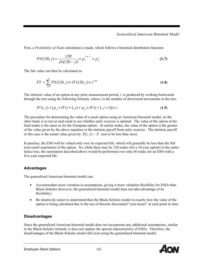
First, a Probability of Node calculation is made, which follows a binomial distribution function:

jdu pp

jjjPN

j

××−×

=− )120(

)!120(!!120),120( (1.7)

The fair value can then be calculated as:

120

0),120(),120( vjIVjPNFV

N

j××=∑

=

(1.8)

The intrinsic value of an option at any prior measurement period, i, is produced by working backwards through the tree using the following formula, where j is the number of downward movements in the tree:

vjiIVpjiIVpjiIV du ×++×++×= )]1,1(),1([),( (1.9)

The procedure for determining the value of a stock option using an American binomial model, on the other hand, is to test at each node to see whether early exercise is optimal. The value of the option at the final nodes is the same as for the European option. At earlier nodes, the value of the option is the greater of the value given by the above equation or the intrinsic payoff from early exercise. The intrinsic payoff in this case is the actual value given by XjiS −),( (not to be less than zero).

In practice, the ESO will be valued only over its expected life, which will generally be less than the full term (until expiration) of the option. So, while there may be 120 nodes (for a 10-year option) in the entire lattice tree, the summation described above would be performed over only 60 nodes for an ESO with a five-year expected life.

Advantages

The generalized American binomial model can:

• Accommodate more variation in assumptions, giving it more valuation flexibility for ESOs than Black-Scholes (however, the generalized binomial model does not take advantage of its flexibility)

• Be intuitively easier to understand than the Black-Scholes model in exactly how the value of the option is being calculated due to the use of discrete discounted “coin tosses” at each point in time

Disadvantages

Since the generalized American binomial model does not incorporate any additional assumptions, similar to the Black-Scholes formula, it does not capture the special characteristics of ESOs. Therefore, the disadvantages of the Black-Scholes model still exist using the generalized binomial model.


Aon Consulting Refined Binomial Model

Description

The Aon Consulting Refined Binomial Model is a refinement of the generalized American binomial model that incorporates more variables.

Refinements

The Aon Consulting Refined Binomial Model incorporates the following unique characteristics:

• Allowance for non-optimal early exercise patterns of the option holders based on truncating branches of the model when the stock price reaches certain price exercise multiples

• A Monte Carlo simulation model that can account for the decay of the fair value of an ESO as its expected life increases

• Illiquidity, due to the lost opportunity cost during the vesting period

Each of the valuation refinements can be used independently of each other or jointly.

• Allowance for non-optimal early exercise patterns of the option holders based on truncating branches of the model when the stock price reaches certain price exercise multiples

Unlike publicly-traded options, ESOs are generally not permitted to be sold or transferred to third parties. To realize a cash benefit or diversify their portfolios, employees must exercise the options and sell the underlying shares. This tends to lead to ESOs being exercised earlier than similar publicly-traded options.

Paragraph 282 of FAS 123 addresses one way to model early exercise behavior, by adjusting the binomial model to assume automatic exercise of an employee option when the modeled stock price is in excess of some multiple, M, of the strike price.

The determination of the exercise multiple is set equal to the average ratio of the stock price to the strike price when employees have made voluntary early exercise decisions in the past and assumes sufficient data is available to calculate the average ratios. The challenge is to determine how the average ratio should be set.

Exercise multiples can vary significantly depending on several factors such as:

Demographics of the option holder Financial status of the option holder Option plan provisions and restrictions Market movements in stock price Market value of stock price



Because of these factors, the data used to set the exercise multiple should be carefully analyzed so that wide variances in historical exercise multiples are not simply combined to arrive at an average. For instance, one analysis may show a multiple among the general employee population of 150% due to concerns for personal financial health (e.g., need for cash). Another analysis may show an exercise multiple of 300% for management due to a deeper knowledge of potential company performance. These analyses must be reconciled in order to make a defensible decision about using an assumption concerning the exercise multiple.

• A Monte Carlo simulation model that can account for the decay of the fair value of an ESO as its expected life increases

Generally, an estimated 50% of the value of an ESO can be found in the first 20% of the option’s lifetime. This occurrence is caused by the increasing decay in value that stock options experience as they age. Through stochastic modeling, using Monte Carlo simulations of the option’s expected life, the impact that changing the expected life has on the fair value of the ESO can be modeled.

Example 3

A company values an ESO with the following assumptions: volatility of 30%, risk-free rate of 4.00%, expected life of six years, no dividend yield, 100% immediate vesting, and no probability of forfeiture.

The table below illustrates the ESO fair values, as a percentage of the grant price, yielded by the Aon Consulting Refined Binomial Model as the exercise multiple is varied.

Exercise Multiple

Fair Values as Percent of Grant Price: Aon Consulting Refined Binomial Model

None 37.4% 550.0% 37.4% 500.0% 37.3% 450.0% 37.3% 400.0% 37.2% 350.0% 37.1% 300.0% 36.7% 250.0% 35.9% 200.0% 34.1% 190.0% 34.1% 180.0% 32.5% 170.0% 32.5% 160.0% 30.3% 150.0% 27.2% 140.0% 27.2% 130.0% 22.8% 120.0% 17.0% 110.0% 9.4% 100.0% 0.0%



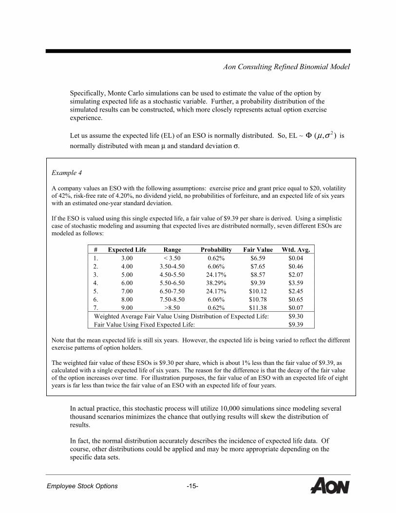
Specifically, Monte Carlo simulations can be used to estimate the value of the option by simulating expected life as a stochastic variable. Further, a probability distribution of the simulated results can be constructed, which more closely represents actual option exercise experience.

Let us assume the expected life (EL) of an ESO is normally distributed. So, EL ∼ Φ ),( 2σµ is normally distributed with mean µ and standard deviation σ.

In actual practice, this stochastic process will utilize 10,000 simulations since modeling several thousand scenarios minimizes the chance that outlying results will skew the distribution of results.

In fact, the normal distribution accurately describes the incidence of expected life data. Of course, other distributions could be applied and may be more appropriate depending on the specific data sets.

Example 4

A company values an ESO with the following assumptions: exercise price and grant price equal to $20, volatility of 42%, risk-free rate of 4.20%, no dividend yield, no probabilities of forfeiture, and an expected life of six years with an estimated one-year standard deviation.

If the ESO is valued using this single expected life, a fair value of $9.39 per share is derived. Using a simplistic case of stochastic modeling and assuming that expected lives are distributed normally, seven different ESOs are modeled as follows:

# Expected Life Range Probability Fair Value Wtd. Avg. 1. 3.00 < 3.50 0.62% $6.59 $0.04 2. 4.00 3.50-4.50 6.06% $7.65 $0.46 3. 5.00 4.50-5.50 24.17% $8.57 $2.07 4. 6.00 5.50-6.50 38.29% $9.39 $3.59 5. 7.00 6.50-7.50 24.17% $10.12 $2.45 6. 8.00 7.50-8.50 6.06% $10.78 $0.65 7. 9.00 >8.50 0.62% $11.38 $0.07 Weighted Average Fair Value Using Distribution of Expected Life: $9.30 Fair Value Using Fixed Expected Life: $9.39

Note that the mean expected life is still six years. However, the expected life is being varied to reflect the different exercise patterns of option holders.

The weighted fair value of these ESOs is $9.30 per share, which is about 1% less than the fair value of $9.39, as calculated with a single expected life of six years. The reason for the difference is that the decay of the fair value of the option increases over time. For illustration purposes, the fair value of an ESO with an expected life of eight years is far less than twice the fair value of an ESO with an expected life of four years.



The mathematics of the normal distribution used for purposes of this stochastic modeling process are briefly summarized in Appendix A.

• Illiquidity, due to the lost opportunity cost during the vesting period

We believe the fair value of an employee stock option is affected by vesting period illiquidity. That is, each time the stock price decreases without the actively employed option holder being permitted to exercise because he is not vested, he loses an opportunity to capture a gain on the stock. However, the new Exposure Draft states that vesting period restrictions do not affect the grant date fair value and should not be considered in the grant date fair value.20

Based on the language in the Exposure Draft, this adjustment may not be included in any financial reporting valuations. If this adjustment were allowable, the economic loss due to the vesting period restrictions would be estimated as follows.

The Aon model calculates the potential loss at each node of the binomial tree prior to vesting. Then, the present value of total economic loss that results from the inability to exercise, when it would have been beneficial to do so, at each of these nodes is calculated.

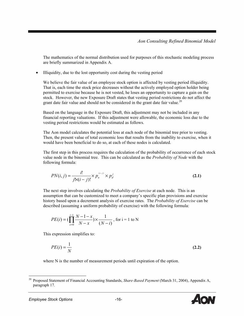
The first step in this process requires the calculation of the probability of occurrence of each stock value node in the binomial tree. This can be calculated as the Probability of Node with the following formula:

jdu pp

jijijiPN

ji

××−×

=− )(

)!(!!),( (2.1)

The next step involves calculating the Probability of Exercise at each node. This is an assumption that can be customized to meet a company’s specific plan provisions and exercise history based upon a decrement analysis of exercise rates. The Probability of Exercise can be described (assuming a uniform probability of exercise) with the following formula:

)(1)1()(

1

0 iNxNxNiPE

i

x −×

−−−= ∏

−

=

, for i = 1 to N

This expression simplifies to:

NiPE 1)( = (2.2)

where N is the number of measurement periods until expiration of the option.

20 Proposed Statement of Financial Accounting Standards, Share-Based Payment (March 31, 2004), Appendix A,

paragraph 17.



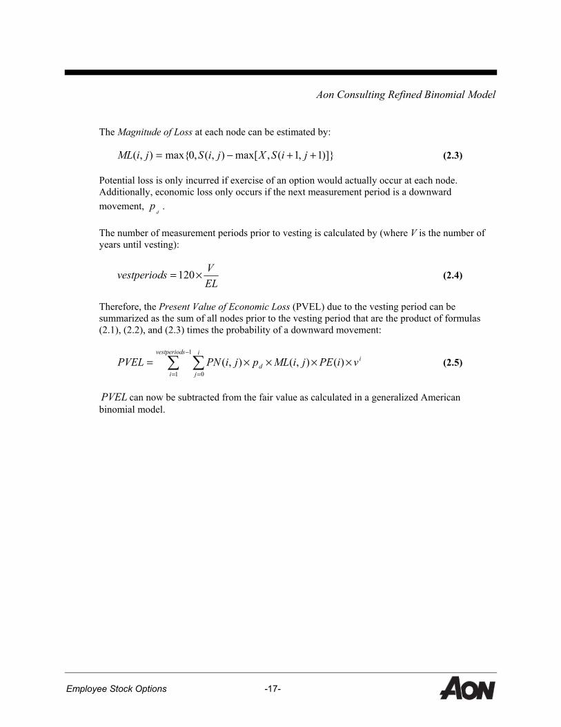
The Magnitude of Loss at each node can be estimated by:

)]}1,1(,max[),(,0max{),( ++−= jiSXjiSjiML (2.3)

Potential loss is only incurred if exercise of an option would actually occur at each node. Additionally, economic loss only occurs if the next measurement period is a downward movement,

dp .

The number of measurement periods prior to vesting is calculated by (where V is the number of years until vesting):

ELVsvestperiod ×= 120 (2.4)

Therefore, the Present Value of Economic Loss (PVEL) due to the vesting period can be summarized as the sum of all nodes prior to the vesting period that are the product of formulas (2.1), (2.2), and (2.3) times the probability of a downward movement:

isvestperiod

i

i

jd viPEjiMLpjiPNPVEL ××××= ∑ ∑

−

= =

1

1 0)(),(),( (2.5)

PVEL can now be subtracted from the fair value as calculated in a generalized American binomial model.



Advantages

The Aon Consulting Refined Binomial Model has the ability to incorporate the following three refinements:

1. Allowance for non-optimal early exercise patterns of the option holders based on truncating branches of the model when the stock price reaches certain exercise multiples

2. A Monte Carlo simulation model that can account for the decay of the fair value of an ESO as its expected life increases

3. Illiquidity, due to the lost opportunity cost during the vesting period

These refinements produce discounts to the option value calculated under the generalized American binomial model. The effect of these refinements is a more accurate representation of the true financial cost of an ESO.

Disadvantage

The Aon Consulting Refined Binomial Model has additional complexity due to the refinements used.

Example 5

A company values an ESO with the following assumptions: volatility of 30%, risk-free rate of 4%, expected life of six years, no dividend yield, no exercise multiple, and no probabilities of forfeiture.

As the following table illustrates, the adjustment for illiquidity during the vesting period can be substantial. The table below compares the fair values as a percentage of the grant price yielded by the Aon Consulting Refined Binomial Model and the traditional American Binomial Model as the vesting period ranges from zero to six years.

Fair Value of Option as Percent of Grant Price

Years to Vesting

Valuation Model 0 1 2 3 4 5 6

Generalized American Binomial 37.4% 37.4% 37.4% 37.4% 37.4% 37.4% 37.4%

Aon Consulting Refined Binomial 37.4% 37.2% 36.7% 36.0% 34.2% 32.1% 25.5%


Aon Consulting Actuarial Binomial Model

Description

The Aon Consulting Actuarial Binomial Model is also a lattice-based model. The primary difference between this model and the Aon Consulting Refined Binomial Model is its ability to reflect exercise patterns of option holders. The Aon Consulting Refined Binomial Model uses exercise patterns only for making the refinements discussed above. Unlike that model, explicit exercise patterns are an inherent component of the Aon Consulting Actuarial Binomial Model. That is, without exercise patterns, this model cannot operate. This additional enhancement further helps to value ESOs with as much precision as possible for financial purposes.

The following is a description of ways that exercise behaviors might be developed for use in a lattice model21:

Lattice models can accommodate information related to exercise and post-vesting termination behavior. Generally, exercise behavior is analyzed by looking at historical exercise information and historical stock prices. That data is analyzed through statistical methods to obtain exercise behavior function that can be incorporated into the lattice model. In addition, that data should be segregated by employee groups to identify homogenous exercise behavior. In addition, an enterprise would have to consider post-vesting termination that results in non-exercise (e.g., because the options are under-water) and its effect on an option’s expected term.

The optimal lattice-based ESO valuation model would incorporate discrete exercise behavior assumptions for each measurement period in the life of the ESO, which would accomplish two goals. First, estimation assumptions (e.g., expected life) that oversimplify exercise behavior could be eliminated. Second, rigorous assumptions that represent exercise behavior could be developed from data relevant to the specific company issuing the options and the option holders. The result would be more accurate and defensible ESO valuations.

Variables

The Aon Consulting Actuarial Binomial Model can incorporate the following variables that influence exercise behaviors:

• Current stock price relative to the strike price

• Time elapsed since vesting

• Time to expiration

• Risk tolerance of the option holder

• Wealth diversification of the option holder 21 Appendix 1 of the FASB Field Visit Discussion Memo on November 10, 2003.



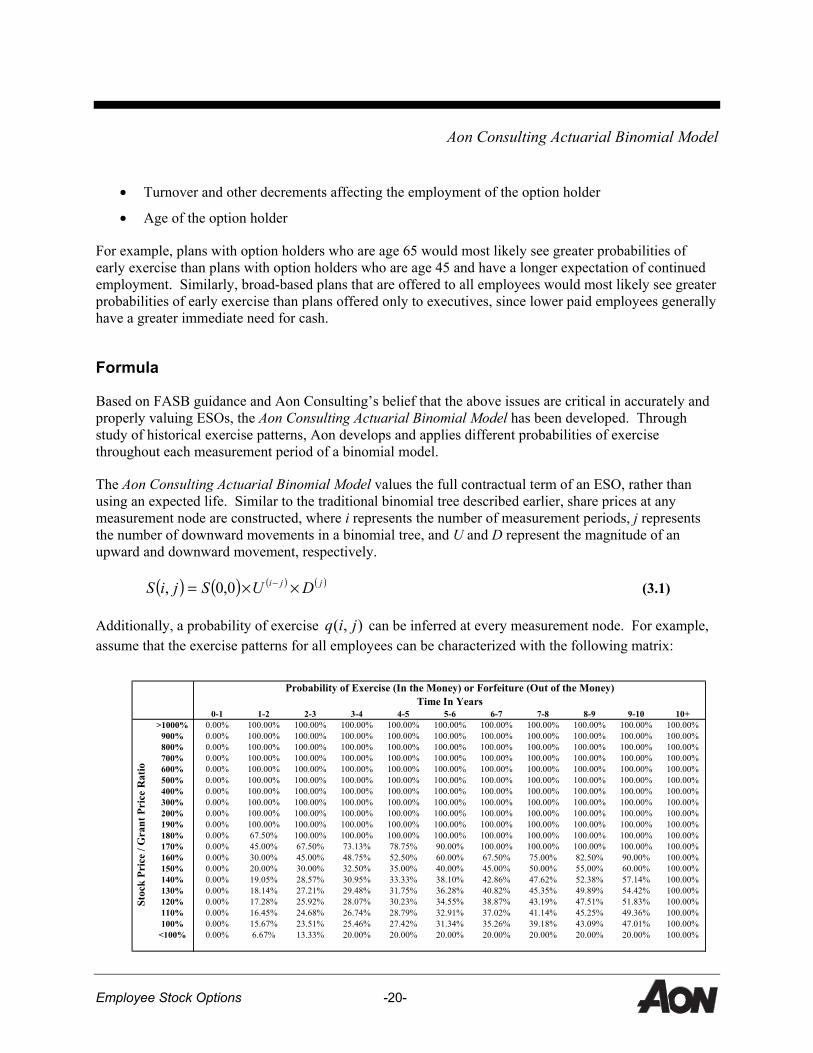
• Turnover and other decrements affecting the employment of the option holder

• Age of the option holder

For example, plans with option holders who are age 65 would most likely see greater probabilities of early exercise than plans with option holders who are age 45 and have a longer expectation of continued employment. Similarly, broad-based plans that are offered to all employees would most likely see greater probabilities of early exercise than plans offered only to executives, since lower paid employees generally have a greater immediate need for cash.

Formula

Based on FASB guidance and Aon Consulting’s belief that the above issues are critical in accurately and properly valuing ESOs, the Aon Consulting Actuarial Binomial Model has been developed. Through study of historical exercise patterns, Aon develops and applies different probabilities of exercise throughout each measurement period of a binomial model.

The Aon Consulting Actuarial Binomial Model values the full contractual term of an ESO, rather than using an expected life. Similar to the traditional binomial tree described earlier, share prices at any measurement node are constructed, where i represents the number of measurement periods, j represents the number of downward movements in a binomial tree, and U and D represent the magnitude of an upward and downward movement, respectively.

( ) ( ) ( ) ( )jji DUSjiS ××= −0,0, (3.1)

Additionally, a probability of exercise ),( jiq can be inferred at every measurement node. For example, assume that the exercise patterns for all employees can be characterized with the following matrix:

0-1 1-2 2-3 3-4 4-5 5-6 6-7 7-8 8-9 9-10 10+>1000% 0.00% 100.00% 100.00% 100.00% 100.00% 100.00% 100.00% 100.00% 100.00% 100.00% 100.00%

900% 0.00% 100.00% 100.00% 100.00% 100.00% 100.00% 100.00% 100.00% 100.00% 100.00% 100.00%800% 0.00% 100.00% 100.00% 100.00% 100.00% 100.00% 100.00% 100.00% 100.00% 100.00% 100.00%700% 0.00% 100.00% 100.00% 100.00% 100.00% 100.00% 100.00% 100.00% 100.00% 100.00% 100.00%600% 0.00% 100.00% 100.00% 100.00% 100.00% 100.00% 100.00% 100.00% 100.00% 100.00% 100.00%500% 0.00% 100.00% 100.00% 100.00% 100.00% 100.00% 100.00% 100.00% 100.00% 100.00% 100.00%400% 0.00% 100.00% 100.00% 100.00% 100.00% 100.00% 100.00% 100.00% 100.00% 100.00% 100.00%300% 0.00% 100.00% 100.00% 100.00% 100.00% 100.00% 100.00% 100.00% 100.00% 100.00% 100.00%200% 0.00% 100.00% 100.00% 100.00% 100.00% 100.00% 100.00% 100.00% 100.00% 100.00% 100.00%190% 0.00% 100.00% 100.00% 100.00% 100.00% 100.00% 100.00% 100.00% 100.00% 100.00% 100.00%180% 0.00% 67.50% 100.00% 100.00% 100.00% 100.00% 100.00% 100.00% 100.00% 100.00% 100.00%170% 0.00% 45.00% 67.50% 73.13% 78.75% 90.00% 100.00% 100.00% 100.00% 100.00% 100.00%160% 0.00% 30.00% 45.00% 48.75% 52.50% 60.00% 67.50% 75.00% 82.50% 90.00% 100.00%150% 0.00% 20.00% 30.00% 32.50% 35.00% 40.00% 45.00% 50.00% 55.00% 60.00% 100.00%140% 0.00% 19.05% 28.57% 30.95% 33.33% 38.10% 42.86% 47.62% 52.38% 57.14% 100.00%130% 0.00% 18.14% 27.21% 29.48% 31.75% 36.28% 40.82% 45.35% 49.89% 54.42% 100.00%120% 0.00% 17.28% 25.92% 28.07% 30.23% 34.55% 38.87% 43.19% 47.51% 51.83% 100.00%110% 0.00% 16.45% 24.68% 26.74% 28.79% 32.91% 37.02% 41.14% 45.25% 49.36% 100.00%100% 0.00% 15.67% 23.51% 25.46% 27.42% 31.34% 35.26% 39.18% 43.09% 47.01% 100.00%

<100% 0.00% 6.67% 13.33% 20.00% 20.00% 20.00% 20.00% 20.00% 20.00% 20.00% 100.00%

Probability of Exercise (In the Money) or Forfeiture (Out of the Money)

Stoc

k Pr

ice

/ Gra

nt P

rice

Rat

io

Time In Years



The preceding matrix summarizes the probability of exercise for all options. When the stock price is “in-the-money” (i.e., ratio > 100%), the probability of exercise is inclusive of all possible triggers for exercise (termination, retirement, cash needs, diversification, etc.). When the stock price is “under-water” there is no probability of exercise. However, there is a probability of vested termination, which would cause the option to be forfeited.

For example, the annualized probability of exercise at ),( jiq is 40%, when the time after grant is five years and the stock price ratio 150%. It is necessary to convert the annualized probability of exercise,

),( jiq , to an incremental probability of exercise, ),( jiq , during the measurement period. Assuming a uniform probability of exercise in each measurement period:

tjiqjiq ∆−−= )),(1(1),( (3.2)

In this example, the incremental probability of exercise when the annualized rate of exercise is 40% (assuming the measurement period is one month long) is:

0417.)40.1(1),( 121

=−−=jiq

After constructing probabilities of exercise at all measurement nodes, the discrete probability of survival, ),( jip , within each measurement period can be determined. A composite function ),(* jipi can then be

defined that incorporates two components: (1) the cumulative probability of survival, ),( jipi , to each measurement period at time i, and (2) the probability of an upward or downward movement, up or dp . Next,

))1,1(1()1,1()),1(1(),1(),( *1

*1

* −−−××−−+−−××−= −− jiqpjipjiqpjipjip diuii

(3.3)



The entire binomial lattice for all (i,j) can be constructed in this manner.

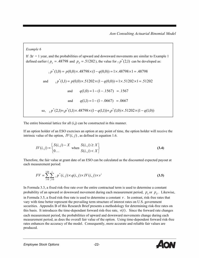
If an option holder of an ESO exercises an option at any point of time, the option holder will receive the intrinsic value of the option, ),( jiIV , as defined in equation 1.6.

−

=K0

),(),(

XjiSjiIV when

<≥

XjiSXjiS

),(),(

(3.4)

Therefore, the fair value at grant date of an ESO can be calculated as the discounted expected payout at each measurement period:

∑∑= =

×××=120

0 0

* ),(),(),(i

ii

ji vjiIVjiqjipFV (3.5)

In Formula 3.3, a fixed risk-free rate over the entire contractual term is used to determine a constant probability of an upward or downward movement during each measurement period, up or dp . Likewise, in Formula 3.5, a fixed risk-free rate is used to determine a constant v . In contrast, risk-free rates that vary with time better represent the prevailing term structure of interest rates on U.S. government securities. Appendix B of this Research Brief presents a methodology for determining risk-free rates on this basis. It introduces the time-dependant forward risk-free rate, )(tv . Since the forward rate changes each measurement period, the probabilities of upward and downward movements change during each measurement period, as does the overall fair value of the option. Using time-dependent forward risk-free rates enhances the accuracy of the model. Consequently, more accurate and reliable fair values are produced.

Example 6

If t∆ = 1 year, and the probabilities of upward and downward movements are similar to Example 1 defined earlier ( 48798.=up and 51202.=dp ), the value for 2 )1,2(*p can be developed as:

48798.148798.1))0,0(1(48798.)0,0()0,1(*1 =××=−××= qpp

and 51202.151202.1))0,0(1(51202.)0,0()1,1(*1 =××=−××= qpp

and 1567.)1567.1(1)0,1( =−−=q

and 0667.)0667.1(1)1,1( =−−=q

so, ))0,1(1(51202.)0,1())1,1(1(48798.)1,1()1,2( *1

*1

*2 qpqpp −××+−××=



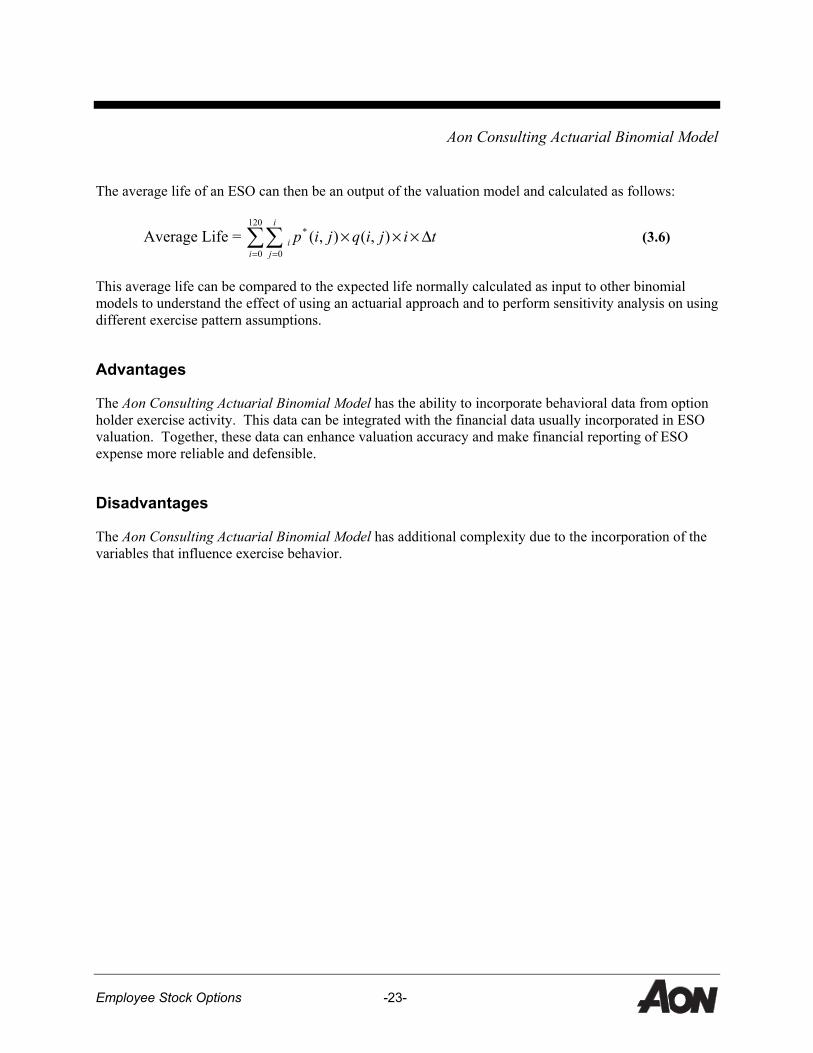
The average life of an ESO can then be an output of the valuation model and calculated as follows:

Average Life = ∑∑= =

∆×××120

0

*

0),(),(

i

i

ji tijiqjip (3.6)

This average life can be compared to the expected life normally calculated as input to other binomial models to understand the effect of using an actuarial approach and to perform sensitivity analysis on using different exercise pattern assumptions.

Advantages

The Aon Consulting Actuarial Binomial Model has the ability to incorporate behavioral data from option holder exercise activity. This data can be integrated with the financial data usually incorporated in ESO valuation. Together, these data can enhance valuation accuracy and make financial reporting of ESO expense more reliable and defensible.

Disadvantages

The Aon Consulting Actuarial Binomial Model has additional complexity due to the incorporation of the variables that influence exercise behavior.


Comparison of Binomial Valuation Models

The preferential use of any of the binomial valuation models needs to be examined under all the facts and circumstances in a given situation. However, with sufficient data, the preferable model will generally be the Aon Consulting Actuarial Binomial Model.

Illustrated below is a comparison of the valuation results of these models.

Example 7

A company values an ESO with the following assumptions: volatility of 30%, risk-free rate of 5%, a 1% dividend yield, one-year vesting, and the following probabilities of exercise:

The Aon Consulting Actuarial Binomial Model yields a fair value per option of 27.36% of grant price and an expected life of 4.10 years, which is approximately similar to historical experience.

Based upon an expected life of 4.10 years and branch truncation at a multiple of 200% of grant price, the Aon Consulting Refined Binomial Model yields a value of 27.30% of grant price.

Finally, both the generalized American binomial model and the traditional Black-Scholes formula yield a value of 29.2% of grant price.

0-1 1-2 2-3 3-4 4-5 5-6 6-7 7-8 8-9 9-10 10+>1000% 0.00% 100.00% 100.00% 100.00% 100.00% 100.00% 100.00% 100.00% 100.00% 100.00% 100.00%

900% 0.00% 100.00% 100.00% 100.00% 100.00% 100.00% 100.00% 100.00% 100.00% 100.00% 100.00%800% 0.00% 100.00% 100.00% 100.00% 100.00% 100.00% 100.00% 100.00% 100.00% 100.00% 100.00%700% 0.00% 100.00% 100.00% 100.00% 100.00% 100.00% 100.00% 100.00% 100.00% 100.00% 100.00%600% 0.00% 100.00% 100.00% 100.00% 100.00% 100.00% 100.00% 100.00% 100.00% 100.00% 100.00%500% 0.00% 100.00% 100.00% 100.00% 100.00% 100.00% 100.00% 100.00% 100.00% 100.00% 100.00%400% 0.00% 100.00% 100.00% 100.00% 100.00% 100.00% 100.00% 100.00% 100.00% 100.00% 100.00%300% 0.00% 100.00% 100.00% 100.00% 100.00% 100.00% 100.00% 100.00% 100.00% 100.00% 100.00%200% 0.00% 100.00% 100.00% 100.00% 100.00% 100.00% 100.00% 100.00% 100.00% 100.00% 100.00%190% 0.00% 100.00% 100.00% 100.00% 100.00% 100.00% 100.00% 100.00% 100.00% 100.00% 100.00%180% 0.00% 67.50% 100.00% 100.00% 100.00% 100.00% 100.00% 100.00% 100.00% 100.00% 100.00%170% 0.00% 45.00% 67.50% 73.13% 78.75% 90.00% 100.00% 100.00% 100.00% 100.00% 100.00%160% 0.00% 30.00% 45.00% 48.75% 52.50% 60.00% 67.50% 75.00% 82.50% 90.00% 100.00%150% 0.00% 20.00% 30.00% 32.50% 35.00% 40.00% 45.00% 50.00% 55.00% 60.00% 100.00%140% 0.00% 19.05% 28.57% 30.95% 33.33% 38.10% 42.86% 47.62% 52.38% 57.14% 100.00%130% 0.00% 18.14% 27.21% 29.48% 31.75% 36.28% 40.82% 45.35% 49.89% 54.42% 100.00%120% 0.00% 17.28% 25.92% 28.07% 30.23% 34.55% 38.87% 43.19% 47.51% 51.83% 100.00%110% 0.00% 16.45% 24.68% 26.74% 28.79% 32.91% 37.02% 41.14% 45.25% 49.36% 100.00%100% 0.00% 15.67% 23.51% 25.46% 27.42% 31.34% 35.26% 39.18% 43.09% 47.01% 100.00%

<100% 0.00% 6.67% 13.33% 20.00% 20.00% 20.00% 20.00% 20.00% 20.00% 20.00% 100.00%

Probability of Exercise (In the Money) or Forfeiture (Out of the Money)

Stoc

k Pr

ice

/ Gra

nt P

rice

Rat

io

Time In Years


Economic Value

This Research Brief is intended to focus on valuing the financial costs of ESOs for accounting purposes. However, it is worthwhile to briefly discuss the concept of economic value and how it may differ from financial statement value.

Economic value is generally referred to as the value that is used to set option award levels. Once the economic value is known, the number of options to be issued can be determined based on the size (in dollars) of the aggregate award pool. Therefore, economic value is the driver in designing the reward program and in communicating the incentive program to employees.

Most organizations calculate economic value using Black-Scholes as the valuation model. As a result, they will generally use the same valuation model they use for calculating the financial statement value. However, there are differences in the assumptions that companies use to determine economic value. While some organizations calculate it by assuming the option is held to expiration (i.e., full term), others determine it using an expected life that is shorter than the full term.

The practical implications of calculating economic value can be debated. Some questions raised are as follows:

• Now that ESOs need to be actually expensed, does the financial statement value need to be reconciled with economic value?

• If economic value is calculated differently than financial statement value, what arguments are used to justify using different methodologies and assumptions?

• How are the many anomalies involved in developing economic value handled? For instance, when the stock price is down (up), how does one keep from awarding too many (too few) options just when one should be doing the opposite?

The economic value can be calculated by recognizing the alignment between the company’s reward intentions and the option holder’s perspective. That is, the company intends to award options in order to create incentives for long-term performance by its employees. This means the employee should hold the option to a point at which its value can be maximized. At this point, the intrinsic value of the stock is the greatest, and exercise at this point gives a payoff that recognizes expected performance. From the option holder’s perspective, he/she wants to enjoy the optimal award available; consequently, exercise at a point when the intrinsic value of the stock is the greatest would be ideal.

The question is when will the value of the option be maximized? The answer depends on whether there is a dividend assumption made in the valuation of the option. If there is no dividend assumption, the theoretical maximum value will be calculated at the terminal point of the option’s life (i.e., 10 years). If there is a dividend assumption, the maximum value will be calculated at the point when the sum of the projected price of the option at time t, plus the accumulated value of dividends at time t, ceases to increase monotonically.

Economic Value


The point at which this occurs will depend on the nature of the dividend payments. In most cases, it will probably not occur before the terminal point of the option’s life. In other cases, it may occur just before the terminal point. This is another reason to use a binomial model to calculate this value, since Black-Scholes will not allow option value measurements at interim points in time before the terminal point.

As financial statement option valuations become more important for proper expensing and disclosure, calculating the economic value will also receive more attention in order that ESO programs can be properly designed and communicated.


Conclusion

The process of calculating fair value for ESOs is relatively new and continually evolving mathematically. A comprehensive fair value analysis of ESO expense will result in greater disclosures in financial statements, more confident shareholders, and satisfied regulatory authorities. Furthermore, the proper valuation of ESOs should mean that fewer companies abandon incentive ESOs for their employees in reaction to accounting rule changes. This Research Brief has described the most accurate approaches currently available for determining the fair value of ESOs. Currently, given sufficient data, the preferable model is the Aon Consulting Actuarial Binomial model.

Aon will continue to refine its models and methodology as financial theory, business practice, and FASB and IASB guidance evolves.


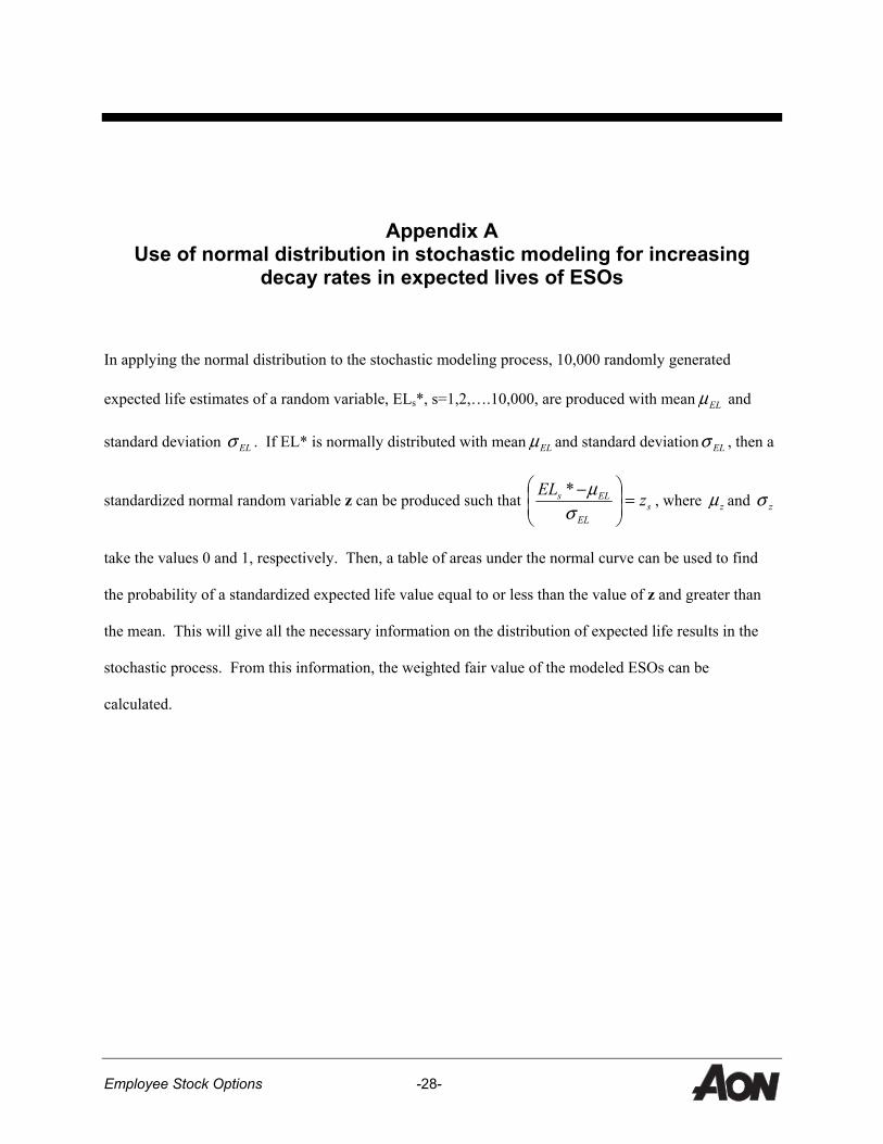
Appendix A Use of normal distribution in stochastic modeling for increasing

decay rates in expected lives of ESOs

In applying the normal distribution to the stochastic modeling process, 10,000 randomly generated

expected life estimates of a random variable, ELs*, s=1,2,….10,000, are produced with mean ELµ and

standard deviation ELσ . If EL* is normally distributed with mean ELµ and standard deviation ELσ , then a

standardized normal random variable z can be produced such that sEL

ELs zEL =

−σ

µ*, where zµ and zσ

take the values 0 and 1, respectively. Then, a table of areas under the normal curve can be used to find

the probability of a standardized expected life value equal to or less than the value of z and greater than

the mean. This will give all the necessary information on the distribution of expected life results in the

stochastic process. From this information, the weighted fair value of the modeled ESOs can be

calculated.


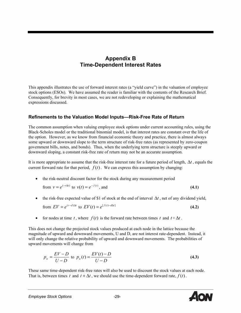
Appendix B Time-Dependent Interest Rates

This appendix illustrates the use of forward interest rates (a “yield curve”) in the valuation of employee stock options (ESOs). We have assumed the reader is familiar with the contents of the Research Brief. Consequently, for brevity in most cases, we are not redeveloping or explaining the mathematical expressions discussed.

Refinements to the Valuation Model Inputs—Risk-Free Rate of Return

The common assumption when valuing employee stock options under current accounting rules, using the Black-Scholes model or the traditional binomial model, is that interest rates are constant over the life of the option. However, as we know from financial economic theory and practice, there is almost always some upward or downward slope to the term structure of risk-free rates (as represented by zero-coupon government bills, notes, and bonds). Thus, when the underlying term structure is steeply upward or downward sloping, a constant risk-free rate of return may not be an accurate assumption.

It is more appropriate to assume that the risk-free interest rate for a future period of length, t∆ , equals the current forward rate for that period, )(tf . We can express this assumption by changing:

• the risk-neutral discount factor for the stock during any measurement period

from )( trev ∆−= to )()( tfetv −= , and (4.1)

• the risk-free expected value of $1 of stock at the end of interval t∆ , net of any dividend yield,

from tdreEV ∆−= )( to ])([)( tdtfetEV ∆−= (4.2)

• for nodes at time t , where )(tf is the forward rate between times t and t + t∆ .

This does not change the projected stock values produced at each node in the lattice because the magnitude of upward and downward movements, U and D, are not interest rate-dependent. Instead, it will only change the relative probability of upward and downward movements. The probabilities of upward movements will change from

DUDEVpu −

−= to DU

DtEVtpu −−= )()( (4.3)

These same time-dependent risk-free rates will also be used to discount the stock values at each node. That is, between times t and tt ∆+ , we should use the time-dependent forward rate, )(tf .

Appendix B

Time-Dependent Interest Rates


Determining Forward Rates

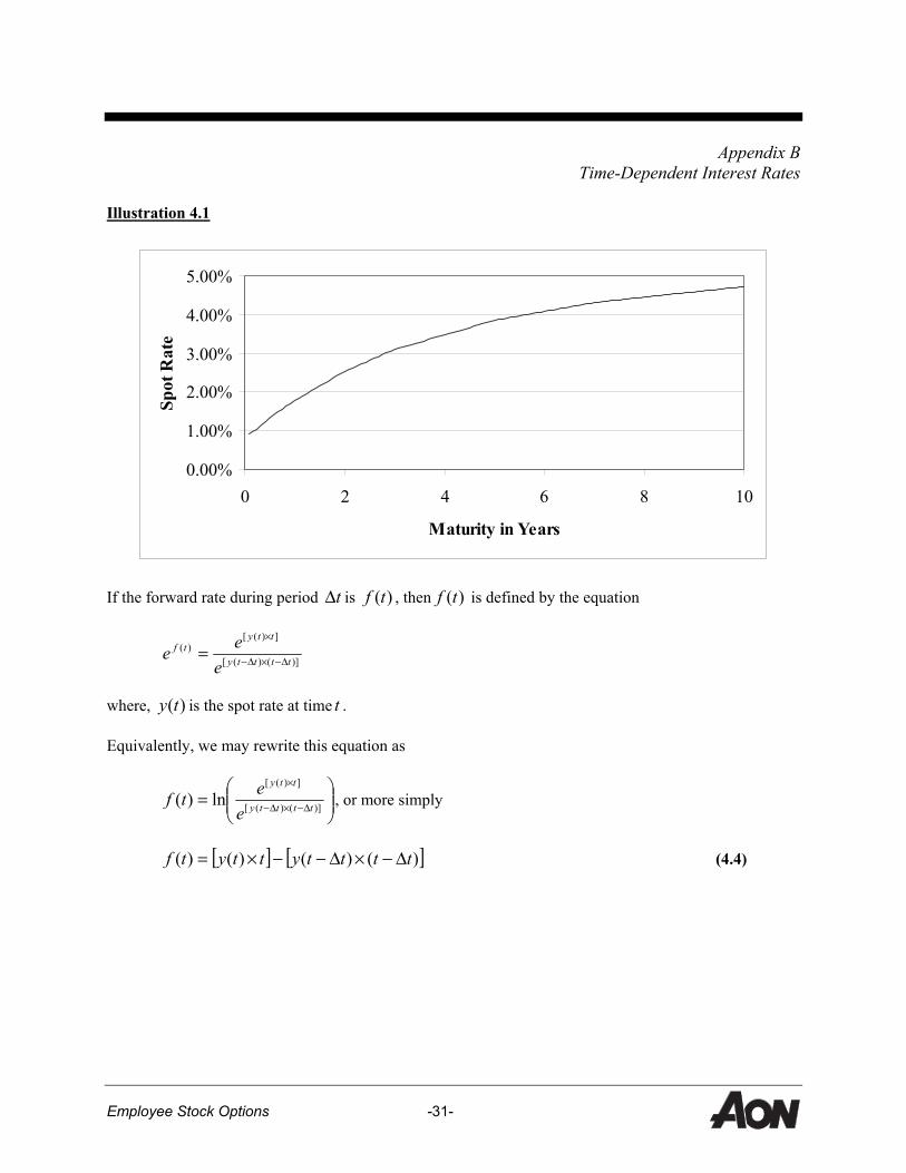
Forward interest rates are the risk-free rates of interest implied from the current U.S. Treasury zero-coupon yield curve for the periods of time that cover the term of the option. The yield to maturity on a zero-coupon bond is sometimes called the spot rate that prevails today for a period corresponding to the maturity of the bond and can be expressed as ( )ty . Illustration 4.1 (below) depicts the yield curve developed, based on May 2004 Treasury rates.

Bond yields are published only for certain maturities. In order to develop a yield curve, interpolated values need to be calculated that represent the convexity (concavity) properties inherent in the term structure of rates. For interpolation purposes, we are using the method of cubic splines. Cubic splines allow us to fit individual third-degree polynomials to the distance between each contiguous set of two nodes in the term structure. In this case, for simplicity and to ensure that we are replicating the published rates exactly, we are using the published rates at the nodes. From the fitted polynomial, we are able to calculate any interpolated risk-free interest rate required for use in the binomial model.

We have chosen the method of cubic splines because it contains the property equality of ordinates, first and second derivatives for the adjacent polynomials (i.e., splines) at the common node. This produces a high degree of smoothness, especially when anomalies arise in published rates that could cause additional inflection points along the produced curve.

An understanding of the mathematics of cubic spline interpolation is not critical to the topic of this Research Brief.

Illustration 4.1 below is based on this interpolation method.

`

Appendix B



Illustration 4.1

0.00%

1.00%

2.00%

3.00%

4.00%

5.00%

0 2 4 6 8 10

Maturity in Years

Spot

Rat

e

If the forward rate during period t∆ is )(tf , then )(tf is defined by the equation

)]()([

])([)(

tttty

ttytf

eee ∆−×∆−

×

=

where, )(ty is the spot rate at time t .

Equivalently, we may rewrite this equation as

= ∆−×∆−

×

)]()([

])([

ln)( tttty

tty

eetf , or more simply

[ ] [ ])()()()( ttttyttytf ∆−×∆−−×= (4.4)

Appendix B



Example 4.1—Calculating a forward rate

U.S. Treasury zero-coupon issues published for May 2004 are as follows:

Maturity Yield 1-Month 0.91% 3-Month 1.04% 6-Month 1.33% 1-Year 1.78% 2-Year 2.53% 3-Year 3.10% 5-Year 3.85% 7-Year 4.31%

10-Year 20-Year

4.72% 5.46%

A yield curve is constructed using the known spot rates and implied spot rates based on interpolated values. (See Illustration 4.1.)

Assume that 0833.0=∆t (1-month), and we are looking to determine the forward rate at the 60th month, ( )0000.5f . Using the yield curve, we find %83.3)9167.4( =y and %85.3)0000.5( =y . Thus,

[ ] [ ])()()()( ttttyttytf ∆−×∆−−×=

( ) ( )9167.4%83.30000.5%85.3 ×−×= , and

%42.0)00.5( =f , which is the forward rate in the 60th month.

Each of the forward rates in the yield curve will be constructed with this approach. We can then apply each of those rates in our binomial model at each of the discrete t∆ time periods.

Example 4.2—Difference in fair market valuation between a fixed risk-free rate and time-dependent risk-free rates

A company values an employee stock option with the following assumptions: volatility of 30%, a fixed risk-free rate of 3.51% (which is commensurate to an average life of the option of 4.1 years for May, 2004 Treasuries), a 1% dividend yield, and probabilities of exercise summarized below. This yields a fair value of an option of 25.77% of grant price.

Alternatively, after substituting the yield curve summarized in Example 4.1 for the fixed risk-free rate, the fair value of an option is 25.46% of grant price.

Since the yield curve in the above example has a positive slope, we would anticipate a lower valuation through the use of a yield curve than a fixed risk-free rate based on an average life.

About Aon Consulting Aon Consulting is among the world’s top global human capital and management consulting firms, providing a complete array of consulting, outsourcing, and insurance brokerage services. In addition, Aon Consulting provides specialized services for various industry sectors, including health care, technology, government, pharmaceuticals, retail, manufacturing, financial services, and public sector. These services help companies of all sizes to attract and retain top talent and improve performance:

Employee Benefits

Compensation and rewards

Process Improvement and Redesign, including Six Sigma

Selection, assessment, and development

Human Resources Outsourcing

Communication

Specialized research, including:

Employee Commitment Compensation and Benefits Customer Loyalty

Aon Consulting professionals possess extensive knowledge and experience in a variety of fields including actuarial science, business, computer science, employee benefits, industrial psychology, organizational behavior, information systems, employment compliance, process improvement design, communication, and leadership development. Headquartered in Chicago, Aon Consulting is the consulting arm of Aon Corporation (NYSE:AOC), a holding company that is comprised of a family of insurance brokerage, consulting, and insurance underwriting subsidiaries. Aon serves clients through 600 offices and 51,000 employees around the world. For more information about the services available from Aon Consulting, call 1.800.438.6487 or visit our Web site at www.aon.com/hcc.

Aon Consulting U.S. Offices ARIZONA • Phoenix CALIFORNIA • Fresno, Irvine, Los Angeles, Sacramento, San Francisco, San Jose COLORADO • Denver CONNECTICUT • Avon, Greenwich, Hartford, Stamford DISTRICT OF COLUMBIA FLORIDA • Jacksonville, Miami, Tampa GEORGIA • Atlanta HAWAII • Honolulu ILLINOIS • Chicago, Rolling Meadows INDIANA • Indianapolis IOWA • Cedar Rapids

KENTUCKY • Louisville MARYLAND • Baltimore, Bethesda, Owings Mills MASSACHUSETTS • Boston, Lexington, Newburyport, Wellesley MICHIGAN • Ann Arbor, Detroit, Grand Rapids MINNESOTA • Minneapolis MISSOURI • Kansas City, St. Louis NEBRASKA • Omaha NEW JERSEY • Lyndhurst, Parsippany, Somerset NEW MEXICO • Albuquerque, Santa Fe NEW YORK • Melville, New York City, Syracuse

NORTH CAROLINA • Charlotte, Raleigh, Winston-Salem OHIO • Cincinnati, Cleveland, Columbus, Findlay OKLAHOMA • Tulsa OREGON • Portland PENNSYLVANIA • Philadelphia, Pittsburgh TENNESSEE • Nashville TEXAS • Austin, Dallas, Fort Worth, Houston UTAH • Salt Lake City VIRGINIA• Richmond, Vienna WASHINGTON • Seattle WISCONSIN • Green Bay, Milwaukee

In addition, we offer services in countries around the world.

We periodically publish Research Briefs and Outlooks on specific topics or trends affecting Aon Consulting clients. Our most recent Research Briefs and Outlooks include:

• On Track Retirement BenchmarkSM: Evaluating Employees’ Financial Readiness for Retirement—November 2004 • HSAs: A New Approach Involving Consumers—October 2004

• Practical Steps to Controlling Medical Costs—May 2004 • Employee Stock Options: An Analysis of Valuation Methods—May 2004

• Retiree Health Benefits—The Divergent Paths—March 2004 • HRWatch: A Focus on Administration—October 2003

• HRWatch: A Focus on Workforce Selection and Development—October 2003 • Domestic Partner Benefits: An Employer’s Perspective—October 2003

• HRWatch: A Focus on Communication—September 2003 • HRWatch: A Focus on Compensation—September 2003

• HRWatch: A Focus on Benefits—September 2003 • Using Captives to Fund Benefits—August 2003

• Electronic Plan Administration Standards—July 2003 • Savings Plan Options for Tax-Exempt Employers: §401(k) vs. §403(b) vs. §457(b) Plans—May 2003

• How to Maximize 401(k) Savings While Minimizing Costs—December 2002 • Consumer-Driven Health Care—November 2002

• HIPAA Privacy and EDI: Employer Compliance Strategies—October 2002 • Fiduciary Fundamentals Under ERISA—August 2002

• Health Care Cost Management: A Strategic Look at 2002 and Beyond—April 2002 • What’s Happening to Retirement Benefit Plans? A Strategic Look at 2002 and Beyond—January 2002

• Health Insurance Portability and Accountability Act of 1996: Assessing the Impact—October 2001 • Electronic Plan Administration Standards—September 2001

• Phased Retirement: A Strategy for Retaining Top Talent—March 2001 • Performance-Based Retirement Benefits—November 2000

• Defined Contribution Health Plans: Future or Fad?—September 2000 • How to Maximize 401(k) Savings While Minimizing Costs—May 2000

• Prescription Drugs in a Managed Care World—February 2000 • Managing Absences by Integrating HR Policies and Benefit Plans—September 1999

• Going Online with Benefits—December 1998 • Medicare+Choice: Challenges and Opportunities—November 1998

• Mergers & Acquisitions: Employee Benefits Due Diligence—June 1998 Please visit our Web site, www.aon.com, to learn more about these and other publications.

To receive a free copy of these briefs, please call 800-438-6487

valuation services - employee stock options - an analysis ... · pdf fileemployee stock...

Documents