valuation of employee stock options (esos) by means of
TRANSCRIPT

Valuation of Employee Stock Options (ESOs) by means ofMean-Variance Hedging
Kamil Kladí[email protected]
andMihail Zervos
Department of Mathematics, London School of Economics
June 25, 2018
Abstract
We consider the problem of ESO valuation in continuous time. In particular, we considermodels that assume that an appropriate random time serves as a proxy for anything thatcauses the ESO’s holder to exercise the option early, namely, reflects the ESO holder’s jobtermination risk as well as early exercise behaviour. In this context, we study the problemof ESO valuation by means of mean-variance hedging. Our analysis is based on dynamicprogramming and uses PDE techniques. We also express the ESO’s value that we derive asthe expected discounted payoff that the ESO yields with respect to an equivalent martingalemeasure, which does not coincide with the minimal martingale measure or the variance-optimal measure. Furthermore, we present a numerical study that illustrates aspects orour theoretical results.
Keywords: employee stock options, mean-variance hedging, classical solutions of PDEs.
AMS subject classifications: 35Q93, 91G10, 91G20, 91G80.
1
arX
iv:1
710.
0089
7v1
[q-
fin.
PR]
2 O
ct 2
017
1 Introduction
Employee stock options are call options granted by a firm to its employees as a form of a benefitin addition to salary. Typical examples of ESO payoff functions F include the one of a call optionwith strike K, in which case, F (s) = (s−K)+, as well as the payoff of a capped call option thatpays out no more than the double of its strike, in which case, F (s) =
(s ∧ (2K) −K
)+. ESOs
are typically long-dated options with maturities up to several years. Also, they typically have avesting period of up to several years, during which, they cannot be exercised. After the expiryof their vesting period, they are of American type.
The International Financial Reporting Standards Board and Financial Accounting StandardsBoard require companies to recognise an ESO as an expense in the income statement at themoment the option is granted. In particular, the fair-value principle is required for an ESOvaluation. Such requirements as well as fundamental differences between ESOs and standardtraded options that we discuss below have generated substantial interest in the development ofmethodologies tailored to ESO valuation.
The risk-neutral valuation approach is a standard way of pricing traded stock options. How-ever, this methodology does not apply to ESOs, primarily, for the following two reasons:
(I ) If ESO holders have their jobs terminated (voluntarily or because of being fired), theyforfeit their unvested ESOs, while they have a short time (typically, up to a few months) toexercise their vested ESOs. The possibility of job termination presents an additional uncertaintyinto the structure of an ESO, which is referred to as the job termination risk .
(II ) ESOs are not allowed to be sold by their holders. Furthermore, ESO holders facerestrictions in trading their employers’ stocks. Therefore, they cannot hedge the initial valuesof their granted ESOs or use them as loss protections for speculation on their underlying stockprice declines. These trading restrictions make ESO holders, who may be in a need for liquidityor want to diversify their portfolios, to exercise ESOs earlier than dictated by risk-neutrality.The early exercise behaviour has been documented in the empirical literature (e.g., see Huddartand Lang [12]), and has be explained theoretically by means of expected utility maximisationtechniques (e.g., see Sircar and Xiong [27]).
A standard way of modelling the job termination risk and the early exercise behaviour isby means of a Poisson process: the ESO is liquidated , namely, exercised if vested and in-the-money or forfeited if unvested or out-of-the money, when the first jump of the Poisson processoccurs. This approach was introduced by Jennergren and Näslund [15], and appears in themajority of ESO valuation models, which can be classified in three main groups. Models inthe first group use the first Poisson jump to capture both the job termination risk and thevoluntary decision of the ESO holder to exercise (e.g., see Rubinstein [23], Carpenter [5], Carrand Linetsky [7], and Sircar and Xiong [27]). Models in the second group use the first Poissonjump to capture the job termination risk, while they impose a barrier that, when reached by thestock price, the ESO’s exercise is triggered (e.g., see Hull and White [13], and Cvitanic, Wienerand Zapatero [9]). Models in these groups can be viewed as of an exogenous or reduced formtype. Models in the third group, which can be viewed as of an endogenous or structural type,use the first Poisson jump to capture the job termination risk but determine the ESO holder’searly exercise strategy by maximising the holder’s utility of personal wealth (e.g., see Leung and
2

Sircar [19], and Carpenter, Stanton and Wallace [6]). The extensive use of a Poisson process inESO valuation has the attractive feature that, in its simplest form, it involves a single parameter,namely, its intensity rate, which can be estimated from historical data on ESO exercises andforfeitures. Indeed, the empirical study in Carpenter [5] shows that a reduced form model withconstant intensity of jumps can perform as well or even better than more elaborate structuralmodels.
In this paper, we study a model that belongs to the first family of models discussed above.In particular, we consider an ESO with maturity T that is written on an underlying stock priceprocess S, which is modelled by a geometric Brownian motion. We denote by F the ESO’spayoff function and we assume that the ESO is vested at time Tv ∈ [0, T ). In the spirit of Carrand Linetsky [7], we model the job termination risk as well as the voluntary decision of the ESOholder to exercise, namely, the ESO’s liquidation time, by means of a random time η with hazardrate that is a function of the ESO’s underlying stock price. In this context, the ESO’s valuationhas to rely on an incomplete market pricing methodology (see Rheinlander and Sexton [22] fora textbook).
The super-replication value of the ESO is obtained by viewing the random liquidation timeη as a discretionary stopping time and treating the ESO as a standard American option. Ac-cordingly, this value is given by
xsr = sup%
EQ1[e−r(%∧T )F (S%∧T )1Tv≤%
], (1)
where Q1 is the minimal martingale measure and the supremum is taken over all stopping times% (see also Remark 1). The super-replication value of an ESO is unrealistically high becauseit does not take into account issues such as the the job termination risk or the early exercisebehaviour discussed above. Indeed, it is this observation that has given rise to the whole researchliterature on the subject.
Another approach is to assign a value to the ESO by computing its expected discountedpayoff with respect to a martingale measure. For instance, we can assign the risk-neutral value
xrn = EQ1[e−r(η∧T )F (Sη∧T )1Tv≤η
](2)
to the ESO, where Q1 is the minimal martingale measure, which, in the context we considerhere, coincides with the variance-optimal martingale measure (see Remarks 1 and 4). Such achoice was proposed by Jennergren and Näslund [15] and Carr and Linetsky [7] by appealingto a diversification argument that amounts to assuming that the jump risk is non-priced. Thereasoning behind this diversification assumption is that a firm grants ESOs to a large numberof employees, whose early exercises and forfeitures are independent of each other.
Here, we study the mean-variance hedging of the ESO’s payoff. The use of quadratic cri-teria to measure the quality of a hedging strategy in continuous time has been proposed byBouleau and Lamberton [4]. Mean-variance hedging was first studied in a specific frameworkby Schweizer [24] and has been extensively studied since then by means of martingale theoryand L2 projections (e.g., see Pham [21], Schweizer [25], and Černý and Kallsen [8]), by meansof PDEs (e.g., see Bertsimas, Kogan and Lo [1]) as well as by means of BSDEs (e.g., see Mania
3

and Tevzadze [20], and Jeanblanc, Mania, Santacroce and Schweizer [14]). Beyond such indica-tive references, we refer to Schweizer [26] for a survey of the vast literature on the subject. Inparticular, we consider the optimisation problem
minimise EP[e−r(η∧T )
[Xx,πη∧T − F (Sη∧T )1Tv≤η
]2]
over (x, π), (3)
where Xx,π is the value process of an admissible self-financing portfolio strategy π that startswith initial endowment x and P is the natural probability measure. We derive the solution tothis problem by first solving the problem
minimise EP[e−r(η∧T )
[Xx,πη∧T − F (Sη∧T )1Tv≤η
]2]
over π, (4)
for any given initial endowment x and then optimising over x. It turns out that the equivalentmartingale measure for the valuation of the ESO’s payoff that arises from the solution to themean-variance optimisation problems given by (3)–(4) is different from the coinciding in thiscontext minimal martingale measure and mean-variance martingale measure (see Remarks 1–4). This discrepancy can be attributed to the fact that market incompleteness is due to therandom time horizon η. Furthermore, it is worth noting that, although the solution to (4) istime-consistent, the solution to (3) is time-inconsistent (see also Remark 2).
The paper is organised as follows. In Section 2, we formulate the problem of ESO mean-variance hedging in continuous time. In Section 3, we derive a classical solution to the problem’sHamilton-Jacobi-Bellman (HJB) equation, which takes the form of a nonlinear parabolic partialdifferential equation (PDE). We establish the main results on the mean-variance hedging of anESO’s payoff in Section 4. Finally, we present a numerical investigation in Section 5.
2 ESO mean-variance hedging
We build the model that we study in this section on a complete probability space (Ω,G,P)carrying a standard one-dimensional Brownian motion W as well as an independent randomvariable U that has the uniform distribution on [0, 1]. We denote by (Ft) the natural filtrationof W , augmented by the P-negligible sets in G. In this probabilistic setting, we consider a firmwhose stock price process S is modelled by the geometric Brownian motion
dSt = µSt dt+ σSt dWt, S0 = s > 0, (5)
where µ and σ 6= 0 are given constants. We assume that the firm can trade their own stock andhas access to a risk-free asset whose unit initialised price is given by
dBt = rBt dt, B0 = 1,
where r ≥ 0 is a constant. The value process of a self-financing portfolio with a position inthe firm’s stock and a position in the risk-free asset that starts with initial endowment x hasdynamics given by
dXt =(rXt + σϑπt
)dt+ σπt dWt, X0 = x, (6)
4
where πt is the amount of money invested in stock at time t and ϑ = (µ − r)/σ is the marketprice of risk.1 We restrict our attention to admissible portfolio strategies, which are introducedby the following definition.
Definition 1. Given a time horizon T > 0, a portfolio process π is admissible if it is (Ft)-progressively measurable and
EP[∫ T
0
π2t dt
]<∞. (7)
We denote by AT the family of all such portfolio processes.
At time 0, the firm issues an ESO that expires at time T and is vested at time Tv ∈ [0, T ),meaning that the ESO can be exercised at any time between Tv and T . We denote by F (S) thepayoff of the ESO. The firm estimates that the holder of the ESO will either exercise it or havetheir job terminated at a random time η. We model this time by
η = inf
t ≥ 0
∣∣∣ exp
(−∫ t
0
`(u, Su) du
)≤ U
,
where the intensity function ` satisfies the assumptions stated in Lemma 1 below. We note thatthe independence of U and F∞ imply that
P(η > t | Ft) = P(U < exp
(−∫ t
0
`(u, Su) du
) ∣∣∣ Ft) = exp
(−∫ t
0
`(u, Su) du
).
We also denote by (Gt) the filtration derived by rendering right-continuous the filtration definedby Ft ∨ σ
(η ≤ s, s ≤ t
), for t ≥ 0. It is a standard exercise of the credit risk theory to show
that the process M defined by
Mt = 1η≤t −∫ t∧η
0
`(u, Su) du (8)
is a (Gt)-martingale.
Remark 1. We will consider probability measures that are equivalent to P and are parametrisedby (Ft)-predictable processes γ > 0 satisfying suitable integrability conditions (see Blanchet-Scalliet, El Karoui and Martellini [2], and Blanchet-Scalliet and Jeanblanc [3]). Given such aprocess, the solution to the SDE
dLγt = (γt− − 1)Lγt− dMt − ϑLγt dWt,
where M is the (Gt)-martingale defined by (8), which is given by
Lγt = exp
(1η≤t ln γη −
∫ t∧η
0
`(u, Su)(γu − 1
)du− 1
2ϑ2t− ϑWt
),
1Subject to suitable assumptions, the analysis we develop can be trivially modified to allow for µ, σ and rto be functions of t and St. However, we opted against such a generalisation because this would complicatesubstantially the notation.
5

defines an exponential martingale. If we denote by Qγ the probability measure on (Ω,GT ) that
has Radon-Nikodym derivative with respect to P given by dQγdP
∣∣∣GT
= LγT , then Girsanov’s theorem
implies that the process(Wt, t ∈ [0, T ]
)is a standard Brownian motion under Qγ, while the
process(Mt, t ∈ [0, T ]
)is a martingale under Qγ, where
Wt = ϑt+Wt and Mt = 1η≤t −∫ t∧η
0
`(u, Su)γu du, for t ∈ [0, T ].
Furthermore, the dynamics of the stock price process are given by
dSt = rSt dt+ σSt dWt, for t ∈ [0, T ], S0 = s > 0,
while the conditional distribution of η is given by
Qγ(η > t | Ft) = exp
(−∫ t
0
`(u, Su)γu du
), for t ∈ [0, T ].
In this context, the choice γ = 1 gives rise to the minimal martingale measure, which co-incides with the variance-optimal martingale measure (see Blanchet-Scalliet, El Karoui andMartellini [2], and Szimayer [28]).
In the probabilistic setting that we have developed, we consider a firm whose objective is toinvest an initial amount x in a self-financing portfolio with a view to hedging against the payoffF (Sη) that they have to pay the ESO’s holder at time η. To this end, a risk-neutral valuationapproach is not possible due to the market’s incompleteness. We therefore consider minimisingthe expected squared hedging error , which gives rise to the following stochastic control problem.
Given an ESO with expiry date T that is vested at time Tv ∈ [0, T ), the objective is tominimise the performance criterion
JT,x,s(π) = EP[e−rηXη
210≤η<Tv +
e−r(η∧T )
[Xη∧T − F (Sη∧T )
]2
1Tv≤η
]= EP
[e−2r(η∧T )
[Xη∧T − F (Sη∧T )1Tv≤η
]2](9)
over all admissible self-financing portfolio strategies. In view of the underlying probabilisticsetting, this performance index admits the expression
JT,x,s(π) = EP[∫ T
0
e−Λt`(t, St)[Xt − F (St)1Tv≤t
]2dt+ e−ΛT
[XT − F (ST )
]2]. (10)
where
Λt = 2rt+
∫ t
0
`(u, Su) du.
The value function of the resulting optimisation problem is defined by
v(T, x, s) = infπ∈AT
JT,x,s(π). (11)
6

3 A classical solution to the HJB equation
In view of standard stochastic control theory, the value function v should identify with a solutionw to the HJB PDE
−wτ (τ, x, s) + infπ
1
2σ2π2wxx(τ, x, s) + σ2sπwxs(τ, x, s) + (rx+ σϑπ)wx(τ, x, s)
+
1
2σ2s2wss(τ, x, s) + µsws(τ, x, s)−
(2r + λ(τ, s)
)w(τ, x, s)
+ λ(τ, s)[x− F (s)1τ≤T−Tv
]2= 0 (12)
that satisfies the initial condition
w(0, x, s) =[x− F (s)
]2, (13)
where the independent variable τ = T − t denotes time-to-maturity and
λ(τ, s) = `(T − τ, s). (14)
If the function w(τ, ·, s) is convex for all (τ, s) ∈ [0, T ] × R+, then the infimum in this PDE isachieved by
π†(τ, x, s) = −σswxs(τ, x, s) + ϑwx(τ, x, s)
σwxx(τ, x, s). (15)
and (12) is equivalent to
−wτ (τ, x, s)−(σswxs(τ, x, s) + ϑwx(τ, x, s)
)2
2wxx(τ, x, s)+
1
2σ2s2wss(τ, x, s) + rxwx(τ, x, s)
+ µsws(τ, x, s)−(2r + λ(τ, s)
)w(τ, x, s) + λ(τ, s)
[x− F (s)1τ≤T−Tv
]2= 0. (16)
In view of the quadratic structure of the problem we consider, we look for a solution to this PDEof the form
w(τ, x, s) = f(τ, s)[x− g(τ, s)
]2+ h(τ, s), (17)
for some functions f , g and h. Substituting this expression for w in (16), we can see that thefunctions f , g and h should satisfy the PDEs
−fτ (τ, s) +1
2σ2s2fss(τ, s) + µsfs(τ, s)− λ(τ, s)f(τ, s) + λ(τ, s)
−(σsfs(τ, s) + ϑf(τ, s)
)2
f(τ, s)= 0, (18)
−gτ (τ, s) +1
2σ2s2gss(τ, s) + rsgs(τ, s)−
(r +
λ(τ, s)
f(τ, s)
)g(τ, s)
+λ(τ, s)F (s)1τ≤T−Tv
f(τ, s)= 0, (19)
−hτ (τ, s) +1
2σ2s2hss(τ, s) + µshs(τ, s)−
(2r + λ(τ, s)
)h(τ, s)
+ λ(τ, s)[F (s)1τ≤T−Tv − g(τ, s)
]2= 0 (20)
7

in (0, T ]× (0,∞), with initial conditions
f(0, s) = 1, g(0, s) = F (s) and h(0, s) = 0. (21)
The following result addresses the solvability of these PDEs as well as certain estimates wewill need.
Theorem 1. Suppose that the functions λ and F are C1 and there exist constants λ, KF > 0and ξ ≥ 1 such that
0 ≤ λ(τ, s) + s∣∣λs(τ, s)∣∣ ≤ λ for all τ, s > 0 (22)
and 0 ≤ F (s) + s∣∣F ′(s)∣∣ ≤ KF
(1 + sξ
)for all s > 0. (23)
The following statements hold true:
(I) The PDE (18) with the corresponding boundary condition in (21) has a C1,2 solution suchthat
¯Kf ≤ f(τ, s) ≤ Kf for all τ ∈ [0, T ] and s > 0 (24)
and∣∣fs(τ, s)∣∣ ≤ Kfs
−1 for all τ ∈ [0, T ] and s > 0, (25)
for some constants¯Kf =
¯Kf (T ) > 0 and Kf = Kf (T ) >
¯Kf .
(II) The PDE (19) with the corresponding boundary condition in (21) has a C1,2 solution suchthat
0 ≤ g(τ, s) ≤ Kg
(1 + sξ
)for all τ ∈ [0, T ] and s > 0 (26)
and∣∣gs(τ, s)∣∣ ≤ Kg
(1 + sξ
)s−1 for all τ ∈ [0, T ] and s > 0, (27)
for some constant Kg = Kg(T ) > 0.
(III) The PDE (20) with the corresponding boundary condition in (21) has a C1,2 solution suchthat
0 ≤ h(τ, s) ≤ Kh
(1 + s2ξ
)for all τ ∈ [0, T ] and s > 0, (28)
for some constant Kh = Kh(T ) > 0.
Proof. We establish each of the parts sequentially.
Proof of (I). If we define
f(τ, s) = φ−1(τ, s), for τ ∈ [0, T ] and s > 0, (29)
then we can see that f satisfies the PDE (18) in (0, T ] × (0,∞) with the corresponding initialcondition in (21) if and only if φ satisfies the PDE
−φτ (τ, s) +1
2σ2s2φss(τ, s) + (r − σϑ)sφs(τ, s)−
(λ(τ, s)φ(τ, s)− λ(τ, s)− ϑ2
)φ(τ, s) = 0 (30)
8

in (0, T ]× (0,∞) with initial condition
φ(0, s) = 1, for s > 0. (31)
Furthermore, if we write
φ(τ, s) = e(λ+ϑ2)τϕ(τ, ln s), for τ ∈ [0, T ] and s > 0, (32)
for some function (τ, z) 7→ ϕ(τ, z), where λ is as in (22), then we can check that φ satisfies thePDE (30) with initial condition (31) if and only if ϕ satisfies the PDE
−ϕτ (τ, z) +1
2σ2ϕzz(τ, z) +
(r − σϑ− 1
2σ2
)ϕz(τ, z)
−(e(λ+ϑ2)τλ(τ, ez)ϕ(τ, z) + λ− λ(τ, ez)
)ϕ(τ, z) = 0 (33)
in (0, T ]× R with initial condition
ϕ(0, z) = 1, for z ∈ R. (34)
To solve this nonlinear PDE, we consider the family of linear PDEs
−ϕψτ (τ, z) +1
2σ2ϕψzz(τ, z) +
(r − σϑ− 1
2σ2
)ϕψz (τ, z)− δψ(τ, z)ϕψ(τ, z) = 0 (35)
in (0, T ]× (0,∞) with initial condition
ϕψ(0, z) = 1, for z ∈ R, (36)
which is parametrised by smooth positive functions ψ, where
δψ(τ, z) = e(λ+ϑ2)τλ(τ, ez)ψ(τ, z) + λ− λ(τ, ez) ≥ 0, for τ ∈ [0, T ] and z ∈ R. (37)
In particular, we note that a solution to (33) satisfies (35) for ψ = ϕ.Consider a C1,2 function ψ satisfying
0 ≤ ψ(τ, z) ≤ 1 and |ψz(τ, z)| ≤ C1 for all τ ∈ [0, T ] and z ∈ R, (38)
for some constant C1 = C1(T ). The properties of such a function and the assumptions on λ implythat there exists a unique C1,2 function ϕψ of polynomial growth that solves the Cauchy problem(35)–(36) (see Friedman [10, Section 6.4] or Friedman [11, Section 1.7]). In view of the Feynman-Kac formula (see Friedman [10, Section 6.5] or Karatzas and Shreve [16, Theorem 5.7.6]), thisfunction admits the probabilistic representation
ϕψ(τ, z) = E[exp
(−∫ τ
0
δψ(τ − u, Zu) du) ∣∣∣ Z0 = z
]∈ (0, 1], for τ ∈ [0, T ] and z ∈ R, (39)
9

where Z is the Brownian motion with drift given by
dZt =
(r − σϑ− 1
2σ2
)dt+ σ dBt, (40)
for some standard one-dimensional Brownian motion B. The assumptions on ψ imply that ϕψzis C1,2 (see Friedman [11, Section 3.5]). Differentiating (35), we can see that ϕψz satisfies
−ϕψτz(τ, z) +1
2σ2ϕψzzz(τ, z) +
(r − σϑ− 1
2σ2
)ϕψzz(τ, z)− δψ(τ, z)ϕψz (τ, z)
−(e(λ+ϑ2)τezλs(τ, e
z)ψ(τ, z) + e(λ+ϑ2)τλ(τ, ez)ψz(τ, z)− ezλs(τ, ez))ϕψ(τ, z) = 0
in (0, T ]× R. Using the Feynman-Kac formula, Jensen’s inequality, (22), (38) and (39), we cansee that ∣∣ϕψz (τ, z)
∣∣ ≤ E[∫ τ
0
exp
(−∫ u
0
δψ(τ − q, Zq) dq)
×(e(λ+ϑ2)(τ−u)eZu
∣∣λs(τ − u, eZu)∣∣ψ(τ − u, Zu)
+ e(λ+ϑ2)(τ−u)λ(τ − u, eZu)∣∣ψz(τ − u, Zu)∣∣
+ eZu∣∣λs(τ − u, eZu)
∣∣)ϕψ(τ − u, Zu) du∣∣∣ Z0 = z
]≤∫ τ
0
λ(
(1 + C1)e(λ+ϑ2)(τ−u) + 1)du
≤ λ(1 + C1)
λ+ ϑ2e(λ+ϑ2)T + λT for all τ ∈ [0, T ] and z ∈ R,
where Z is the Brownian motion with drift given by (40). It follows that ϕψ inherits all of theproperties that we have assumed for ψ above. Furthermore, Schauder’s interior estimates forparabolic PDEs implies that, given any bounded open interval I ⊂ R,
‖ϕψ‖(0,T )×I1+a,2+a ≤ C2 sup
τ∈(0,T ), z∈I
∣∣ϕψ(τ, z)∣∣ ≤ C2, (41)
where
‖ϕ‖D1+a,2+a = ‖ϕ‖Da + ‖ϕt‖Da + ‖ϕz‖Da + ‖ϕzz‖Da ,
‖ϕ‖Da = sup(t,z)∈D
|ϕ(t, z)|+ sup(t,z),(t′,z′)∈D(t,z)6=(t′,z′)
|ϕ(t, z)− ϕ(t′, z′)||t− t′|a/2 + |z − z′|a
,
and C2 depends only on a and I (see Friedman [11, Section 3.2]).To proceed further, we denote by ϕ(0) the solution to (35)–(36) for ψ ≡ 0 and by ϕ(j+1) the
solution to (35)–(36) for ψ = ϕ(j) and j ≥ 0. By appealing to a simple induction argument, wecan see that each ϕ(j) has all of the properties that we assumed for ψ in the previous paragraph.
10

Therefore, all of the functions ϕ(j), j ≥ 0, satisfy the estimates (41) for the same constant C2.This observation and the Arzelà-Ascoli theorem imply that there exist a C1,2 function ϕ and asequence of natural numbers (jn) such that
ϕ(jn) −→n→∞
ϕ, ϕ(jn)t −→
n→∞ϕt, ϕ(jn)
z −→n→∞
ϕz and ϕ(jn)zz −→
n→∞ϕzz,
uniformly on compacts. Such a limiting function is a solution to (35)–(36) for ψ = ϕ, namely,a solution to the nonlinear PDE (33) that satisfies the initial condition (34). Furthermore, ϕzsatisfies the PDE
−ϕτz(τ, z) +1
2σ2ϕzzz(τ, z) +
(r − σϑ− 1
2σ2
)ϕzz(τ, z)
−(
2e(λ+ϑ2)τλ(τ, ez)ϕ(τ, z) + λ− λ(τ, ez))ϕz(τ, z)
−ezλs(τ, ez)(e(λ+ϑ2)τϕ(τ, z)− 1
)ϕ(τ, z) = 0
in (0,∞)× R. It follows that the function φ given by (32) is such that φs satisfies the PDE
−φτs(τ, s) +1
2σ2s2φsss(τ, s) +
(r − σϑ+ σ2
)sφss(τ, s)
−(2λ(τ, s)φ(τ, s)− λ(τ, s)− r − ϑ2 + σϑ
)φs(τ, s)− λs(τ, s) (φ(τ, s)− 1)φ(τ, s) = 0 (42)
in (0, T ]× (0,∞), as well as the boundary condition
φs(0, s) = 0, for s > 0. (43)
To establish (24)–(25), we first note that (39) yields the representations
ϕ(0)(τ, z) = E[exp
(−∫ τ
0
δ0(τ − u, Zu) du) ∣∣∣ Z0 = z
]and ϕ(j+1)(τ, z) = E
[exp
(−∫ τ
0
δϕ(j)
(τ − u, Zu) du) ∣∣∣ Z0 = z
], (44)
for τ ∈ [0, T ], z ∈ R and j ≥ 0, where Z is the Brownian motion with drift given by (40).Combining these expressions with the definition (37) of the functions δϕ
(j), we can see that
ϕ(0) > ϕ(1) ⇒ −δϕ(0)
< −δϕ(1) ⇒ ϕ(1) < ϕ(2),
ϕ(1) < ϕ(2) ⇒ −δϕ(1)
> −δϕ(2) ⇒ ϕ(2) > ϕ(3),
ϕ(0) > ϕ(2) ⇒ −δϕ(0)
< −δϕ(2) ⇒ ϕ(1) < ϕ(3),
and ϕ(1) < ϕ(3) ⇒ −δϕ(1)
> −δϕ(3) ⇒ ϕ(2) > ϕ(4).
Iterating these observations, we can see that the sequence of functions (ϕ(2j)) is strictly decreas-ing, while the sequence of functions (ϕ(2j+1)) is strictly increasing. It follows that
ϕ(1) ≤ ϕ ≤ ϕ(0) ≤ 1. (45)
11

In view of (22) and (44), we calculate
ϕ(1)(τ, z) ≥ E[exp
(−∫ τ
0
(e(λ+ϑ2)(τ−u)λ(τ − u, eZu) + λ− λ(τ − u, eZu)
)du
) ∣∣∣ Z0 = z
]≥ exp
(−λ∫ τ
0
e(λ+ϑ2)(τ−u) du
)≥ exp
(−e(λ+ϑ2)τ
)for all τ ∈ [0, T ] and z ∈ R. (46)
Combining the inequalities (45) and (46) with (29) and (32), we obtain (24).Using the Feynman-Kac formula, Jensen’s inequality, (22), (32) and (45), we can see that
the solution to (42)–(43) satisfies∣∣φs(τ, s)∣∣ ≤ E[∫ τ
0
exp
(−∫ u
0
(2λ(τ − q, Sq)φ(τ − q, s)− λ(τ − q, Sq)− r − ϑ2 + σϑ
)dq
)×∣∣λs(τ − u, Su)∣∣ (φ(τ − u, Su) + 1
)φ(τ − u, Su) du
∣∣∣ S0 = s
]≤ λe(λ+ϑ2)τ E
[∫ τ
0
e(r−σϑ)uS−1u
(e(λ+ϑ2)(τ−u) + 1
)du∣∣∣ S0 = s
]= λe(λ+ϑ2)τs−1
∫ τ
0
(e(λ+ϑ2)(τ−u) + 1
)du
≤ 2e2(λ+ϑ2)τs−1 for all τ ∈ [0, T ] and s > 0, (47)
where S is the geometric Brownian motion given by
dSt = (r − σϑ+ σ2)St dt+ σSt dBt,
for a standard one-dimensional Brownian motion B. Combining this estimate with (29), (32),(45) and (46), we obtain
∣∣fs(τ, s)∣∣ =
∣∣φs(τ, s)∣∣φ2(τ, s)
≤ 2 exp(
2e(λ+ϑ2)τ)s−1 for all τ ∈ [0, T ] and s > 0,
and (25) follows.
Proof of (II). If we write
g(τ, s) = g(τ, ln s), for τ ≥ 0 and s > 0,
for some function (τ, z) 7→ g(τ, z), then g satisfies the PDE (19) in (0, T ] × (0,∞) with thecorresponding initial condition in (21) if and only if g satisfies the PDE
−gτ (τ, z) +1
2σ2gzz(τ, z) +
(r − 1
2σ2
)gz(τ, z)
−(r + e(λ+ϑ2)τλ(τ, ez)ϕ(τ, z)
)g(τ, z) + e(λ+ϑ2)τλ(τ, ez)ϕ(τ, z)F (ez)1τ≤T−Tv = 0,
12

in (0, T ]× R, where ϕ is introduced by (32), with initial condition
g(0, z) = F (ez), for z ∈ R.
In view of the assumptions on λ, F , and the smoothness and boundedness of ϕ that we haveestablished above, there exists a unique C1,2 function g of polynomial growth that solves thisCauchy problem (see Friedman [11, Section 1.7]).
In view of the Feynman-Kac formula (Friedman [10, Section 6.5] or Karatzas and Shreve [16,Theorem 5.7.6]), the solution to the PDE (19) with the corresponding initial condition in (21)admits the probabilistic expression
g(τ, s) = E[ ∫ τ
0
exp
(−∫ u
0
(r +
λ(τ − q, Sq)f(τ − q, Sq)
)dq
)λ(τ − u, Su)F (Su)1τ−u≤T−Tv
f(τ − u, Su)du
+ exp
(−∫ τ
0
(r +
λ(τ − u, Su)f(τ − u, Su)
)du
)F (Sτ )
∣∣∣ S0 = s
]≥ 0 for all τ ∈ [0, T ] and s > 0, (48)
where S is the geometric Brownian motion given by
dSt = rSt dt+ σSt dBt, (49)
for a standard one-dimensional Brownian motion B. Using (22)–(24), we can see that thisexpression implies that
g(τ, s) ≤ E[∫ τ
0
λ¯K−1f KF (1 + Sξu) du+KF (1 + Sξτ )
∣∣∣ S0 = s
]=
∫ τ
0
λ¯K−1f KF
(1 + sξe(
12σ2ξ(ξ−1)+rξ)u
)du
+KF
(1 + sξe(
12σ2ξ(ξ−1)+rξ)τ
)for all τ ∈ [0, T ] and s > 0.
It follows that g admits an upper bound as in (26).Similarly to the proof of (I) above, we can verify that gs satisfies the PDE
−gτs(τ, s) +1
2σ2s2gsss(τ, s) + (r + σ2)sgss(τ, s)− λ(τ, s)φ(τ, s)gs(τ, s) + γ(τ, s) = 0, (50)
in (0, T ]× R, where φ is as in (29) and
γ(τ, s) = −[λs(τ, s)φ(τ, s) + λ(τ, s)φs(τ, s)
][g(τ, s)− F (s)1τ≤T−Tv
]+ λ(τ, s)φ(τ, s)F ′(s)1τ≤T−Tv.
Using the relevant bounds in (22), (23), (26), (45) and (47), we calculate∣∣γ(τ, s)∣∣ ≤ (λe(λ+ϑ2)τs−1 + 2λe3(λ+ϑ2)τs−1
)(Kg +KF )(1 + sξ) + λe(λ+ϑ2)τKF (1 + sξ)s−1
≤ Kγ
(1 + sξ
)s−1 for all τ ∈ [0, T ] and s > 0,
13

for some constant Kγ = Kγ(T ) > 0. If we denote by S the geometric Brownian motion given by
dSt = (r + σ2)St dt+ σSt dBt,
where B is a standard one-dimensional Brownian motion, then (50), the Feynman-Kac formula,Jensen’s inequality and the estimate for γ derived above yield
∣∣gs(τ, s)∣∣ ≤ E[∫ τ
0
exp
(−∫ u
0
λ(τ − q, Sq)φ(τ − q, Sq) dq) ∣∣γ(τ − u, Su)
∣∣ du ∣∣∣ S0 = s
]≤ E
[∫ τ
0
Kγ
(S−1u + Sξ−1
u
) ∣∣∣ S0 = s
]= Kγ
∫ τ
0
(s−1e−ru + sξ−1e(
12σ2(ξ−2)+(r+σ2))(ξ−1))u
)du for all τ ∈ [0, T ] and s > 0.
It follows that |gs| admits a bound as in (27).
Proof of (III). We can show that the PDE (20) in (0, T ] × (0,∞) with the correspondinginitial condition in (21) has a C1,2 solution in the same way as in the proof of (II). Usingthe Feynman-Kac formula once again, we can see that this solution admits the probabilisticexpression
h(τ, s) = E[∫ τ
0
exp
(−∫ u
0
(2r + λ(τ − q, Sq)
)dq
)× λ(τ − u, Su)
[F (Su)1τ−u≤T−Tv − g(τ − u, Su)
]2du
]≥ 0, (51)
where S is the geometric Brownian motion given by (5). In view of (22) and (26), we can seethat this expression implies that
h(τ, s) ≤ E[∫ τ
0
2λ(τ − u, Su)[F 2(Su) + g2(τ − u, Su)
]du∣∣∣ S0 = s
]≤ E
[∫ τ
0
4λ[K2F (1 + S2ξ
u ) +K2g (1 + S2ξ
u )]du∣∣∣ S0 = s
]=
∫ τ
0
4λ
[K2F
(1 + s2ξe(σ
2ξ(2ξ−1)+2µξ)u)
+K2g
(1 + s2ξe(σ
2ξ(2ξ−1)+2µξ)u)]du
for all τ ∈ [0, T ] and s > 0, and the claim in (28) follows.
4 The main results on ESO mean-variance hedging
In view of (15) and (17), we can see that the optimal portfolio strategy is given by
π?t = π†(T − t,X?t , St) = −αt
[X?t − g(T − t, St)
]+ Stgs(T − t, St) = −αtX?
t + βt, (52)
14

where π† is the function defined by (15),
αt =σStfs(T − t, St) + ϑf(T − t, St)
σf(T − t, St), βt = αtg(T − t, St) + Stgs(T − t, St), (53)
and X? is the associated solution to (6).The following result presents the solution to the control problem associated with ESO mean-
variance hedging.
Theorem 2. Consider the stochastic control problem defined by (5), (6), (10) and (11), andsuppose that the assumptions of Lemma 1 hold true. The problem’s value function v identifieswith the solution w to the HJB PDE (12)–(13) that is as in (17)–(21), namely,
v(T, x, s) = w(T, x, s) for all x ∈ R and s > 0. (54)
Furthermore, the portfolio strategy π? defined by (52)–(53) is optimal.
Proof. We fix any initial condition (x, s) and any admissible portfolio π ∈ AT . Using Itô’sformula, we calculate∫ t
0
e−Λu`(u, Su)[Xu − F (Su)1Tv≤u
]2du
+ e−Λtw(T − t,Xt, St) = w(T, x, s) + At +Mt, for t ∈ [0, T ], (55)
where
At =
∫ t∧T
0
e−Λu
[−wτ (T − u,Xu, Su) +
1
2σ2π2
uwxx(T − u,Xu, Su)
+ σ2Suπuwxs(T − u,Xu, Su) +1
2σ2S2
uwss(T − u,Xu, Su)
+ (rXu + σϑπu)wx(T − u,Xu, Su) + µSuws(T − u,Xu, Su)
−(2r + `(u, Su)
)w(T − u,Xu, Su) + `(u, Su)
[Xu − F (Su)1Tv≤u
]2]du
and
Mt = σ
∫ t∧T
0
e−Λu[πuwx(T − u,Xu, Su) + Suws(T − u,Xu, Su)
]dWu.
Since w satisfies the PDE (12) and the boundary condition (13), we can see that this identityimplies that
EP[ ∫ T∧Tn
0
e−Λu`(u, Su)[Xu − F (Su)1Tv≤u
]2du
+ e−ΛT[XT − F (ST )
]21T≤Tn + e−ΛTnw(T − Tn, XTn , STn)1Tn<T
]≥ w(T, x, s), (56)
15

where (Tn) is any sequence of localising stopping times for the local martingale M .In view of the estimates in (24), (26) and (28), we can see that∣∣w(τ, x, s)
∣∣ ≤ 2f(τ, s)[x2 + g2(τ, s)
]+ h(τ, s)
≤ Kw
(1 + x2 + s2ξ
)for all τ ∈ [0, T ], x ∈ R and s > 0,
for some constants Kw = Kw(T ) > 0 and ξw > 0. On the other hand, the admissibility condition(7), Fubini’s theorem, Jensen’s inequality and Itô’s isometry imply that
EP[X2t
]= EP
[e2rt
(x+ σϑ
∫ t
0
e−ruπu du+ σ
∫ t
0
e−ruπu dWu
)2]
≤ 9e2rt
(x2 + σ2ϑ2 EP
[(∫ t
0
e−ruπu du
)2]
+ σ2 EP
[(∫ t
0
e−ruπu dWu
)2])
≤ 9e2rt
(x2 + σ2(ϑ2t+ 1)EP
[∫ t
0
e−2ruπ2u du
])<∞
These results imply that the random variable supt∈[0,T ]
∣∣w(T − t,Xt, St)∣∣ is integrable. We can
therefore pass to the limit as n→∞ in (56) using the monotone and the dominated convergencetheorems to obtain
JT,x,s(π) ≡ EP[∫ T
0
e−Λt`(t, St)[Xt − F (St)1Tv≤t
]2dt+ e−ΛT
[XT − F (ST )
]2]≥ w(T, x, s). (57)
Since the initial condition (x, s) and the portfolio strategy π ∈ AT have been arbitrary, it followsthat
v(T, x, s) ≥ w(T, x, s) for all T > 0, x ∈ R and s > 0. (58)
To prove the reverse inequality and establish (54) as well as the optimality of the portfoliostrategy π? defined by (52)–(53), we first show that π? is admissible, namely, π? ∈ AT . To thisend, we first note that
EP [X?t
2]≤ 25
(x2 + EP
[(∫ t
0
(r − σϑαu)X?u du
)2]
+ σ2ϑ2 EP
[(∫ t
0
βu du
)2]
+ σ2 EP[∫ t
0
α2uX
?u
2 du
]+ σ2 EP
[∫ t
0
β2u du
]), (59)
where we have also used Itô’s isometry. The estimates (24)–(25) imply that there exists aconstant Kα = Kα(T ) such that
|αt| ≤σSt∣∣fs(T − t, St)∣∣+ ϑf(T − t, St)
σf(T − t, St)≤ Kα for all t ∈ [0, T ], (60)
16

while the estimates (26)–(27) imply that there exists a constant Kβ = Kβ(T ) such that
β2t ≤ 2α2
t g2(T − t, St) + 2S2
t g2s(T − t, St) ≤ Kβ(1 + S2ξ
t ) for all t ∈ [0, T ]. (61)
Using these inequalities, we can see that, e.g.,
EP[∫ t
0
α2uX
?u
2 du
]≤ K2
α
∫ t
0
EP [X?u
2]du for all t ∈ [0, T ]
and EP
[(∫ t
0
βu du
)2]≤ T EP
[∫ t
0
β2u du
]≤ KβT
(1 +
∫ t
0
EP [S2ξu
]du
)≤ C1(1 + s2ξ) for all t ∈ [0, T ],
where C1 = C1(T ) is a constant. In view of these inequalities and similar ones for the otherterms, we can see that (59) implies that there exists C2 = C2(T, s) such that
EP [X?t
2]≤ C2 + C2
∫ t
0
EP [X?u
2]du.
It follows that
EP [X?t
2]≤ C2e
C2t for all t ∈ [0, T ],
thanks to Grönwall’s inequality. Combining this result with (60) and (61), we obtain
EP[∫ T
0
π?t2 dt
]≤ 2EP
[∫ T
0
(α2tX
?t
2 + β2t
)dt
]≤ 2
∫ T
0
(K2αC2e
C2t +Kβ
(1 + EP
[S2ξt
]))dt <∞,
and the admissibility of π? follows.Finally, it is straightforward to check that the portfolio strategy π? defined by (52)–(53) is
such that (56) as well as (57) hold true with equality, which combined with the inequality (58),implies that π? is optimal and that (54) holds true.
Remark 2. Given an ESO such as the one we have considered, the self-financing portfolio’sinitial endowment X?
0 = x? that minimises the expected squared hedging error is equal tog(T, S0), which is the ESO’s mean-variance hedging value at time 0. It is worth noting thatthe optimal portfolio strategy π? that starts with initial endowment X?
0 = g(T, S0) has valueprocess X? such that X?
t 6= g(T − t, St) (this can be seen by a comparison of the dynamics ofthe processes X? and
(g(T − t, St), t ∈ [0, T ]
)). We can therefore view g(T − t, St) as the ESO’s
mark-to-market mean-variance hedging value at time t.
17

Remark 3. We can express the ESO’s value g(T, s) at time 0 as its expected with respect toa martingale measure discounted cost to the firm. To this end, we consider the exponentialmartingale (Lt, t ∈ [0, T ]) that solves the SDE
dLt =(f−1(T − t, St)− 1
)Lt− dMt − ϑLt dWt,
where M is the (Gt)-martingale defined by (8), and is given by
Lt = exp
(− 1η≤t ln f(T − η, Sη)
−∫ t∧η
0
`(u, Su)(f−1(T − u, Su)− 1
)du− 1
2ϑ2t− ϑWt
), for t ∈ [0, T ].
If we denote by Q the probability measure on (Ω,GT ) that has Radon-Nikodym derivativewith respect to P given by dQ
dP
∣∣GT
= LT , then Girsanov’s theorem implies that the process(Wt, t ∈ [0, T ]
)is a standard Brownian motion under Q, while the process
(Mt, t ∈ [0, T ]
)is a
martingale under Q, where
Wt = ϑt+Wt and Mt = 1η≤t −∫ t∧η
0
`(u, Su)(f−1(T − u, Su)− 1
)du, for t ∈ [0, T ].
Furthermore, the dynamics of the stock price process are given by
dSt = rSt dt+ σSt dWt, for t ∈ [0, T ], S0 = s > 0,
while the conditional distribution of η is given by
Q(η > t | Ft) = exp
(−∫ t
0
`(u, Su)
f(T − u, Su)du
), for t ∈ [0, T ].
In view of these observations and the Feynman-Kac formula (see also (48)–(49) in Appendix I),we can see that
g(T, s) = EQ[∫ T
0
exp
(−∫ t
0
(r +
`(u, Su)
f(T − u, Su)
)du
)`(t, St)F (St)1Tv≤t
f(T − t, St)dt
+ exp
(−∫ T
0
(r +
`(u, Su)
f(T − u, Su)
)du
)F (ST )
]= EQ
[e−r(η∧T )F (Sη∧T )1Tv≤η
], (62)
as claimed at the beginning of the remark.
Remark 4. Suppose that σϑ = µ− r = 0. In this special case, we can check that the constantfunction f ≡ 1 satisfies the PDE (18), the PDE (19) takes the form
−gτ (τ, s) +1
2σ2s2gss(τ, s) + rsgs(τ, s)−
(r + λ(τ, s)
)g(τ, s) + λ(τ, s)F (s)1τ≤T−Tv = 0, (63)
18

the mean-variance hedging value of the ESO is given by
g(T, s) = EP[∫ T
0
e−∫ t0 (r+`(u,Su)) du`(t, St)F (St)1Tv≤t dt+ e−
∫ T0 (r+`(u,Su)) duF (ST )
], (64)
and the optimal portfolio is given by
π?t = Stgs(T − t, St).
Jennergren and Näslund [15] and Carr and Linetsky [7] assume that the ESO’s exercise risk canbe diversified away and propose (64) to be the value of the ESO. Furthermore, they derive thePDE (63) with boundary condition g(0, s) = F (s) by appealing to the Feynman-Kac theorem,and they solve it for the special cases that arise when Tv = 0,
`(T − τ, s) ≡ λ(τ, s) = λf + λe1s>K or `(T − τ, s) ≡ λ(τ, s) = λf + λe(ln s− lnK)+
and F (s) = (s − K)+, for some constants λf , λe, K > 0. Effectively, this approach amountsto choosing the minimal martingale measure for the valuation of the ESO (see also Remark 1).Indeed, in the general case, i.e., when µ 6= r, the function g given by (64) for µ = r identifieswith the function g given by
g(T, s) = EQ1
[∫ T
0
e−∫ t0 (r+`(u,Su)) du`(t, St)F (St)1Tv≤t dt+ e−
∫ T0 (r+`(u,Su)) duF (ST )
]= EQ1
[e−r(η∧T )F (Sη∧T )1Tv≤η
],
where Q1 is the probability measure with Radon-Nikodym derivative with respect to P given bydQ1
dP
∣∣GT
= L1T ≡ exp
(−1
2ϑ2T − ϑWT
).
Remark 5. (The infinite time horizon case.) In many cases, ESOs are very long-dated. It istherefore of interest to consider the form that the solution to the problem we have studied takesas T → ∞. In this case, if Tv = 0 and ` does not depend explicitly on time, then the solutionto the control problem becomes stationary, namely, it does not depend on time. In particular,the value function v∞ identifies with the function w∞ defined by
w∞(x, s) = f∞(s)[x− g∞(s)
]2+ h∞(s),
and the optimal portfolio strategy is given by
π?t = −σStf′∞(St) + ϑf∞(St)
σf∞(St)
[X?t − g∞(St)
]+ Stg
′∞(St),
where X? is the associated solution to (6), and the functions f∞, g∞, h∞ are appropriate solutionsto the ODEs
1
2σ2s2f ′′∞(s) + µsf ′∞(s)− λ(s)f∞(s) + λ(s)−
(σsf ′∞(s) + ϑf∞(s)
)2
f∞(s)= 0, (65)
1
2σ2s2g′′∞(s) + rsg′∞(s)−
(r +
λ(s)
f∞(s)
)g∞(s) +
λ(s)F (s)
f∞(s)= 0, (66)
1
2σ2s2h′′∞(s) + µsh′∞(s)−
(2r + λ(s)
)h∞(s) + λ(s)
[F (s)− g∞(s)
]2= 0. (67)
19

The nonlinear ODE (65) with general λ requires a separate analysis that goes beyond the scopeof this article. For the purposes of this remark, we therefore assume that
` ≡ λ > 0 is a constant, 0 ≤ F (s) ≤ KF
(1 + sξ
)for all s > 0, (68)
λ+ ϑ2 >
(r +
1
2σ2ξ
)(ξ − 1) and λ > 2r(ξ − 1) + 2σϑξ + σ2ξ(2ξ − 1), (69)
where KF > 0 and ξ ≥ 1 are constants. Note that, if ξ = 1, then the inequalities (69) areequivalent to the simpler
λ > 2
(µ− r +
1
2σ2
). (70)
For constant λ, we can verify that the solution to (18) that satisfies the corresponding boundarycondition in (21) is given by
f(τ, s) =λ
λ+ ϑ2+
ϑ2
λ+ ϑ2e−(λ+ϑ2)τ . (71)
In view of this observation, we can see that the constant function given by f∞(s) = λλ+ϑ2
, fors > 0, trivially satisfies (65). Furthermore, (62) and (51) suggest that the functions given by
g∞(s) = (λ+ ϑ2)EQ[∫ ∞
0
e−(r+λ+ϑ2)tF (St) dt
]and h∞(s) = λEP
[∫ ∞0
e−(2r+λ)t[F (St)− g∞(St)
]2dt
]should satisfy the ODEs (66) and (67). Note that the conditions in (68) and (69) are sufficientfor these functions to be real-valued because
g∞(s) ≤ (λ+ ϑ2)KF
∫ ∞0
e−(r+λ+ϑ2)t(
1 + EQ[Sξt ]) dt= (λ+ ϑ2)KF
∫ ∞0
e−(r+λ+ϑ2)t(
1 + sξe(12σ2ξ(ξ−1)+rξ)t
)dt
≤ Kg∞(1 + sξ),
where Kg∞ is a constant, and
h∞(s) ≤ 4λ(K2F +K2
g∞
) ∫ ∞0
e−(2r+λ)t(
1 + EP[S2ξt
])dt
= 4λ(K2F +K2
g∞
) ∫ ∞0
e−(2r+λ)t(
1 + s2ξe(σ2ξ(2ξ−1)+2(σϑ+r)ξ)t
)dt
<∞.
20

In view of standard analytic expressions of resolvents (e.g., see Knudsen, Meister and Zervos [17,Proposition 4.1] or Lamberton and Zervos [18, Theorem 4.2]), these functions admit the analyticexpressions
g∞(s) =λ+ ϑ2
σ2(ng −mg)
[smg
∫ s
0
u−mg−1F (u) du+ sng∫ ∞s
u−ng−1F (u) du
]and h∞(s) =
λ
σ2(nh −mh)
[smh
∫ s
0
u−mh−1[F (u)− g∞(u)
]2du
+ snh∫ ∞s
u−nh−1[F (u)− g∞(u)
]2du
],
where the constants mg < 0 < ng and mh < 0 < nh are defined by
mg, ng = −r − 1
2σ2
σ2∓
√(r − 1
2σ2
σ2
)2
+2
σ2
(r +
λ2
λ+ ϑ2
),
mh, nh = −µ− 1
2σ2
σ2∓
√(µ− 1
2σ2
σ2
)2
+2(2r + λ)
σ2.
We can check that these functions indeed satisfy the ODEs (66) and (67) by direct substitution.It is worth noting that we can use these expressions to calculate g∞ and h∞ in closed analyticform for a most wide range of choices for F .
5 Numerical investigation
We have numerically investigated the stochastic control problems given by (3) and (4) by solvingtheir discrete time counterparts that arise if we approximate the geometric Brownian motion Sby a binomial tree with 1000 time steps. To this end, we have used the same parametrisationas in Section 5 of Carr and Linetsky [7]. In particular, we have considered an ESO grantedat the money (S0 = K = 100), with a ten year maturity (T = 10) and with payoff functionF (s) = max(s−K, 0). Contrary to Carr and Linetsky [7], who consider immediate vesting, wehave assumed a vesting period of three years (Tv = 3). The intensity function ` is given by
`(T − τ, s) ≡ λ(τ, s) = λf + λe(ln s− lnK)+1τ≤T−Tv, for τ ∈ [0, T ] and s > 0,
for λf = λe = 10%. The constants λf and λe account for the ESO holder’s job terminationrisk and the fact that the ESO holder’s desire to exercise increases as the option’s moneynessincreases, respectively. We have assumed that the risk-free rate is 5% and the stock pricevolatility is 30%. Furthermore, we have considered a drift rate of 15% as well as a drift rate of25%.
5.1 The mean-variance frontier
We have solved numerically the recursive equations associated with the discrete time approxi-mation of the problem given by (4). For each x, we have thus computed the expected squared
21

hedging error at the random time of the ESO’s liquidation over all self-financing portfolio strate-gies with initial endowment x. The red parabolas in Figure 1, which we call “mean variancefrontiers”, are plots of the square root of this error, to which we refer as the “root mean squaredhedging error” (RMSHE), against the value of the initial endowment x. The ESO’s mean-variance hedging value at time 0 is denoted by x? and corresponds to the apex of each parabola.
We have also used backward induction to compute the ESO’s risk-neutral value xrn, whichhas been proposed by Carr and Linetsky [7], as well as the ESO’s super-replication value xsr
(see also (1) and (2) in the introduction). In each of these two cases, we have computed thecorresponding RMSHEs using Monte Carlo simulation along the lines described in the nextsubsection, and we have located the associated points in Figure 1.
As expected the ESO’s risk-neutral and super-replication values xrn and xsr do not dependon the drift rate. On the other hand, the ESO’s mean-variance value x? is sensitive to the valueof the market price of risk. Indeed, the two plots in Figure 1 illustrate the dramatic effect thatthe value of the drift rate may have on the ESO’s mean-variance hedging value.
5.2 Distribution of the hedging errors
In the case of mean-variance valuation, we have considered the portfolio strategy that startswith initial capital x?. In the case of risk-neutral valuation, we have considered the standardBlack and Scholes Delta hedging strategy with initial endowment xrn. In the case of super-replication valuation, we have considered the portfolio strategy that starts with xsr and hedgesthe American option that yields the payoff F (Sτ ) if exercised at time τ ∈ [Tv, T ]. In each of the
Figure 1: Mean-variance frontier, initial endowments and RMSHEs.
22
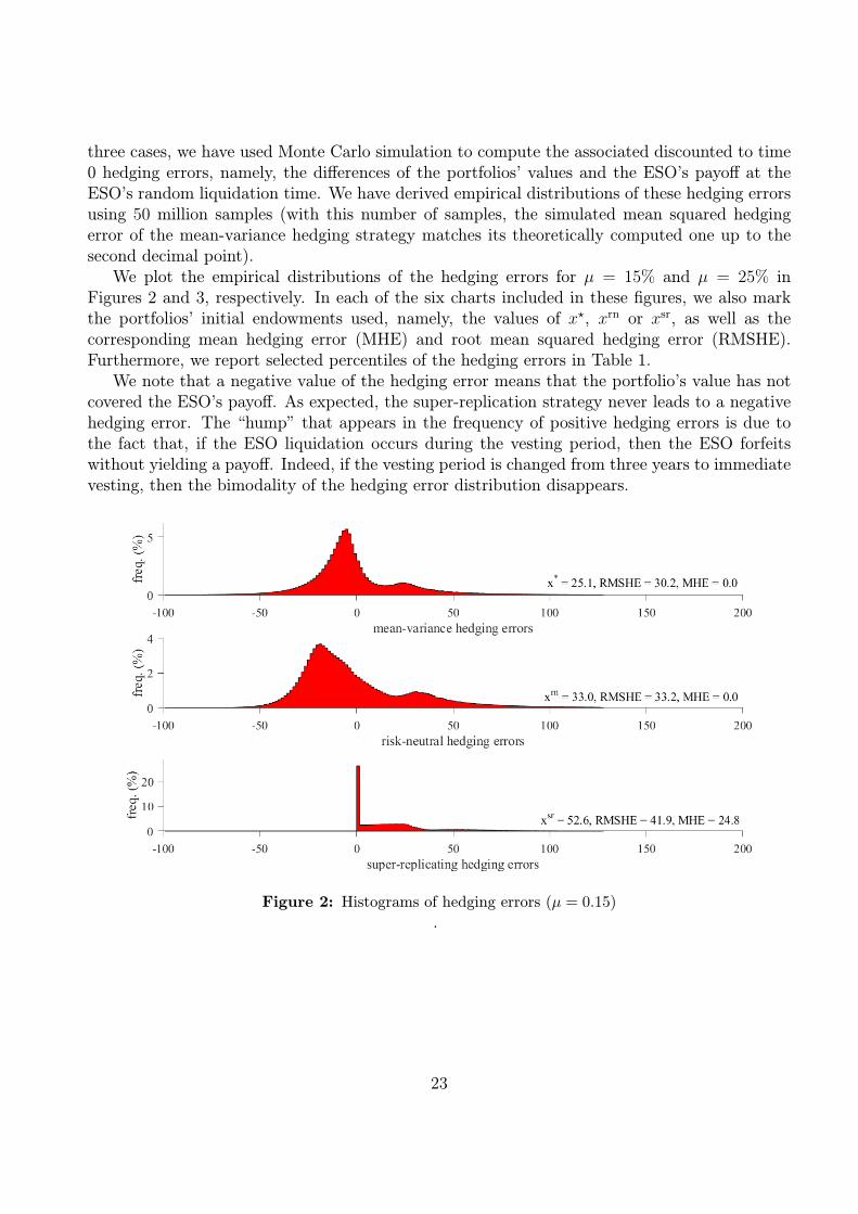
three cases, we have used Monte Carlo simulation to compute the associated discounted to time0 hedging errors, namely, the differences of the portfolios’ values and the ESO’s payoff at theESO’s random liquidation time. We have derived empirical distributions of these hedging errorsusing 50 million samples (with this number of samples, the simulated mean squared hedgingerror of the mean-variance hedging strategy matches its theoretically computed one up to thesecond decimal point).
We plot the empirical distributions of the hedging errors for µ = 15% and µ = 25% inFigures 2 and 3, respectively. In each of the six charts included in these figures, we also markthe portfolios’ initial endowments used, namely, the values of x?, xrn or xsr, as well as thecorresponding mean hedging error (MHE) and root mean squared hedging error (RMSHE).Furthermore, we report selected percentiles of the hedging errors in Table 1.
We note that a negative value of the hedging error means that the portfolio’s value has notcovered the ESO’s payoff. As expected, the super-replication strategy never leads to a negativehedging error. The “hump” that appears in the frequency of positive hedging errors is due tothe fact that, if the ESO liquidation occurs during the vesting period, then the ESO forfeitswithout yielding a payoff. Indeed, if the vesting period is changed from three years to immediatevesting, then the bimodality of the hedging error distribution disappears.
Figure 2: Histograms of hedging errors (µ = 0.15).
23
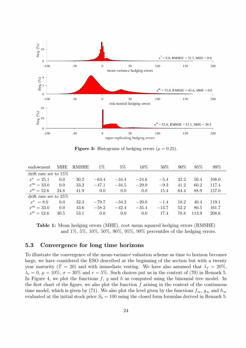
Figure 3: Histograms of hedging errors (µ = 0.25).
endowment MHE RMSHE 1% 5% 10% 50% 90% 95% 99%
drift rate set to 15%x? = 25.1 0.0 30.2 −63.4 −34.4 −24.6 −5.4 32.2 50.4 108.0xrn = 33.0 0.0 33.2 −47.1 −34.5 −29.0 −9.3 41.2 60.2 117.4xsr = 52.6 24.8 41.9 0.0 0.0 0.0 15.4 64.4 88.9 157.0
drift rate set to 25%x? = 8.0 0.0 32.3 −79.7 −34.2 −20.0 −1.4 18.2 40.4 119.1xrn = 33.0 0.0 43.6 −58.2 −42.4 −35.4 −13.7 52.2 80.5 161.7xsr = 52.6 30.5 53.1 0.0 0.0 0.0 17.4 78.8 113.9 208.6
Table 1: Mean hedging errors (MHE), root mean squared hedging errors (RMSHE)and 1%, 5%, 10%, 50%, 90%, 95%, 99% percentiles of the hedging errors.
5.3 Convergence for long time horizons
To illustrate the convergence of the mean-variance valuation scheme as time to horizon becomeslarge, we have considered the ESO described at the beginning of the section but with a twentyyear maturity (T = 20) and with immediate vesting. We have also assumed that λf = 20%,λe = 0, µ = 10%, σ = 30% and r = 5%. Such choices put us in the context of (70) in Remark 5.In Figure 4, we plot the functions f , g and h as computed using the binomial tree model. Inthe first chart of the figure, we also plot the function f arising in the context of the continuoustime model, which is given by (71). We also plot the level given by the functions f∞, g∞ and h∞evaluated at the initial stock price S0 = 100 using the closed form formulas derived in Remark 5.
24

Figure 4: Illustration of convergence for long time horizons.
Acknowledgement
We are grateful to Monique Jeanblanc for several helpful discussions and suggestions. Thefirst author would like to thank the Norwegian School of Economics, the Norske Bank fond tiløkonomisk forskning, and Professor Wilhelm Keilhaus’s minnefond for supporting his researchstay at the LSE.
References
[1] D.Bertsimas, L.Kogan and A. Lo (2001), Hedging derivative securities and incompletemarkets: an ε-arbitrage approach, Operations Research, vol. 49, pp. 372–397.
[2] C.Blanchet-Scalliet, N. El Karoui and L.Martellini (2005), Dynamic asset pric-ing theory with uncertain time-horizon, Journal of Economic Dynamics & Control , vol. 29,pp. 1737–1764.
[3] C.Blanchet-Scalliet and M. Jeanblanc (2004), Hazard rate for credit risk and hedg-ing defaultable contingent claims, Finance and Stochastics , vol. 8, pp. 145–159.
[4] N.Bouleau and D. Lamberton (1989), Residual risks and hedging strategies in Marko-vian markets, Stochastic Processes and their Applications , vol. 33, pp. 131–150.
[5] J.N.Carpenter (1998), The exercise and valuation of executive stock options, Journalof Financial Economics , vol. 48, pp. 127–158.
25
[6] J.N.Carpenter, R. Stanton and N.Wallace (2010), Optimal exercise of execu-tive stock options and implications for firm cost, Journal of Financial Economics , vol. 98,pp. 315–337.
[7] P.Carr and V. Linetsky (2000), The valuation of executive stock options in an intensity-based framework, European Finance Review , vol. 4, pp. 211–230.
[8] A.Černý and J.Kallsen (2007), On the structure of general mean-variance hedgingstrategies, The Annals of Probability , vol. 35, pp. 1479–1531.
[9] J.Cvitanic, Z.Wiener and E. Zapatero (2008), Analytic pricing of employee stockoptions, Review of Financial Studies , vol. 21, pp. 683–724.
[10] A.Friedman (2006), Stochastic Differential Equations and Applications , Dover Publica-tions.
[11] A.Friedman (2008), Partial Differential Equations of Parabolic Type, Dover Publications.
[12] S.Huddart and M.Lang (1996), Employee stock option exercises an empirical analysis,Journal of Accounting and Economics , vol. 21, pp. 5–43.
[13] J.Hull and A.White (2004), How to value employee stock options, Financial AnalystsJournal , vol. 60, pp. 114–119.
[14] M. Jeanblanc, M.Mania, M. Santacroce and MSchweizer (2012), Mean-variancehedging via stochastic control and BSDEs for general semimartingales, The Annals of Ap-plied Probability , vol. 22, pp. 2388–2428.
[15] L.P. Jennergren and B.Näslund (1993), A comment on “valuation of executive stockoptions and the FASB proposal”, The Accounting Review, vol. 68, pp. 179-183.
[16] I. Karatzas and S. E. Shreve (1988), Brownian Motion and Stochastic Calculus ,Springer-Verlag.
[17] T. S.Knudsen, B.Meister and M.Zervos (1998), Valuation of investments in realassets with implications for the stock prices, SIAM Journal on Control and Optimization,vol. 36, pp. 2082–2102.
[18] D.Lamberton and M.Zervos (2013), On the optimal stopping of a one-dimensionaldiffusion, Electronic Journal of Probability , vol. 18, pp. 1–49.
[19] T.Leung and R. Sircar (2009), Accounting for risk aversion, vesting, job terminationrisk and multiple exercises in valuation of employee stock options, Mathematical Finance,vol. 19, pp. 99–128.
[20] M.Mania and R.Tevzadze (2003), A semimartingale backward equation and thevariance-optimal martingale measure under general information flow, SIAM Journal onControl and Optimization, vol. 42, pp. 1703–1726.
26

[21] H.Pham (2000), On quadratic hedging in continuous time, Mathematical Methods of Op-erations Research, vol. 51, pp. 315–339.
[22] T.Rheinlander and J. Sexton (2011), Hedging Derivatives , World Scientific PublishingCo.
[23] M.Rubinstein (1995), On the accounting valuation of employee stock options, The Journalof Derivatives , vol. 3, pp. 8–24.
[24] M.Schweizer (1992), Mean-variance hedging for general claims, Annals of Applied Prob-ability , vol. 2, pp. 171–179.
[25] M.Schweizer (2001), A guided tour through quadratic hedging approaches, in:E. Jouini, J. Cvitanic and M.Musiela (eds.), Option Pricing, Interest Rates and RiskManagement , Cambridge University Press, pp. 538–574.
[26] M.Schweizer (2010), Mean-variance hedging, in R.Cont (ed.), Encyclopedia of Quan-titative Finance, Wiley, pp. 1177–1181.
[27] R. Sircar and W.Xiong (2007), A general framework for evaluating executive stockoptions, Journal of Economic Dynamics and Control , vol. 31, pp. 2317–2349.
[28] A. Szimayer (2004), A reduced form model for ESO valuation Modelling the effects ofemployee departure and takeovers on the value of employee share options, MathematicalMethods of Operations Research, vol. 59, pp. 111–128.
27