155

ID JÁRÁSQuarterly Journal of the Hungarian Meteorological Service

Vol. 112, No. 3–4, July–December 2008, pp. 155–177

Validation of the ALADIN-Climate regional climate model at the Hungarian Meteorological Service

Gabriella Csima* and András Horányi

Hungarian Meteorological Service, P.O. Box 38, H-1525 Budapest, Hungary

E-mails: csima.g@met.hu; horanyi.a@met.hu

(Manuscript received in final form October 28, 2008)

Abstract—Regional climate models are popular and efficient tools for the assessment of the regional aspects of the past and future climate. The application of such models is indispensable for the provision of climate simulations over a smaller region, such as Hungary. The ALADIN-Climate regional climate model was adapted by the Hungarian Meteorological Service in order to derive a regional climate model which can be used efficiently for climate change simulations over Hungary. In this paper three different recent past (1961–2000) regional climate simulations are examined and evaluated: the ERA-40-driven 10 km and 25 km resolution simulations and the ARPEGE-driven 10 km resolution simulation. Based on these investigations, the strengths and weaknesses of the simulations are analyzed in detail in order to understand the behavior and reliability of the ALADIN-Climate model for the past climate. Also, some examination regarding the sensitivity of the model with respect to the domain size and resolution was undertaken. It was demonstrated to what extent the model is capable of simulating the statistical characteristics of the climate for a 30-year period. The results obtained suggest: (1) the ALADIN-Climate model driven by ERA-40 “perfect” lateral boundaries is colder and wetter than reality for the period of 1961–1990, (2) the integration driven by the ARPEGE model slightly improved the results and, furthermore, (3) provided added value to the global model’s results. Additionally it was found that (4) the 25 km simulation on a larger domain provided better results than the 10 km one using a smaller domain, which can be attributed to the fact that 10 km domain is overly small. The results also (5) justify the application of the ALADIN-Climate model for climate change scenario experiments for Hungary.

Key-words: regional climate modeling, ALADIN-Climate model, dynamical downscaling

* Corresponding author

156

1. Introduction

The demand for more spatially and temporally detailed weather and climate information is continuously increasing. This requirement, together with the increased availability of computer power, led to the application of more highly resolved models from the nowcasting to the climate ranges. As far as climate modeling is concerned, global and regional climate models are widely used for the simulation of the past and the future evolution of the climate system. There are three tools that have been successfully applied to bridge the gap between the low resolution global climate models and the regional and local characteristics: variable-resolution global models, statistical downscaling, and dynamical downscaling with regional climate models (RCMs). The first method allows the production of higher resolution climate information without too much additional investment in computer power with respect to the “usual” global simulations (Brankovic and Gregory, 2001; May and Roeckner, 2001; Duffy et al., 2003; Coppola and Giorgi, 2005). Statistical downscaling consists of establishing statistical relationships between large scale (global) parameters as predictors and regional (local) parameters as predictands. These relationships are then applied to the global model outputs (Kattenberg et al., 1996; Hewitson and Crane, 1996; Wilby et al., 2004) and results in information on a regional scale. RCMs, as limited area models, cover only a portion of the planet, typically a continental or even smaller domain (Giorgi and Mearns, 1991; McGregor, 1997; Giorgi andMearns, 1999; Wang et al., 2004). They require lateral boundary conditions (LBCs) obtained from “observations”, such as atmospheric analyses (Uppala et al., 2005), or global simulations. The principal reason for performing regional simulations is to successfully simulate such regional characteristics which are “out of the reach” of the global models, therefore, providing added value through more precise representation of the different surface features, the application of the higher resolution dynamics and improved physical parameterizations.

The ALADIN limited area numerical weather prediction model (Horányi et al., 1996; Horányi et al., 2006) has been developed through an international cooperation and is one of the widely used limited area models in Europe. The ALADIN spectral model family is a very useful tool not only for short range weather prediction, but also for climate range simulations because of its particularly high computational efficiency. Firstly, the original short range version of the model was studied in order to check whether any spurious accumulation of systematic errors (biases) could be detected for longer integrations – it was found not to be the case (Janisková, 1994). Later the ALADIN-Climate model had been created by merging the physical parameterization package of the ARPEGE-Climat global climate model and the dynamics of the ALADIN model. This model was successfully adapted by the Hungarian Meteorological Service in 2005, and it has been used for

157

various climate experiments. Within that framework some shorter time range (3–5 years) experiments have been carried out in order to establish the most appropriate model version, the model domain, the horizontal resolution, and the spin-up time before committing to the first longer time period experiments. This first long-term experiment (1958–2000) has been performed by the Hungarian National Climate Dynamics Programme (www.met.hu/palyazat/nkfp_klima2005.php), and the second one, at a higher horizontal resolution, within the framework of the CECILIA (Central and Eastern Europe Climate Change Impact and Vulnerability Assessment) project(www.cecilia-eu.org).

In Section 2 a brief description of the ALADIN-Climate model is given. Section 3 introduces the model experiments, the evaluation methods, and the observational data used in the present work. Results are presented in Section 4 and the conclusions are drawn in Section 5.

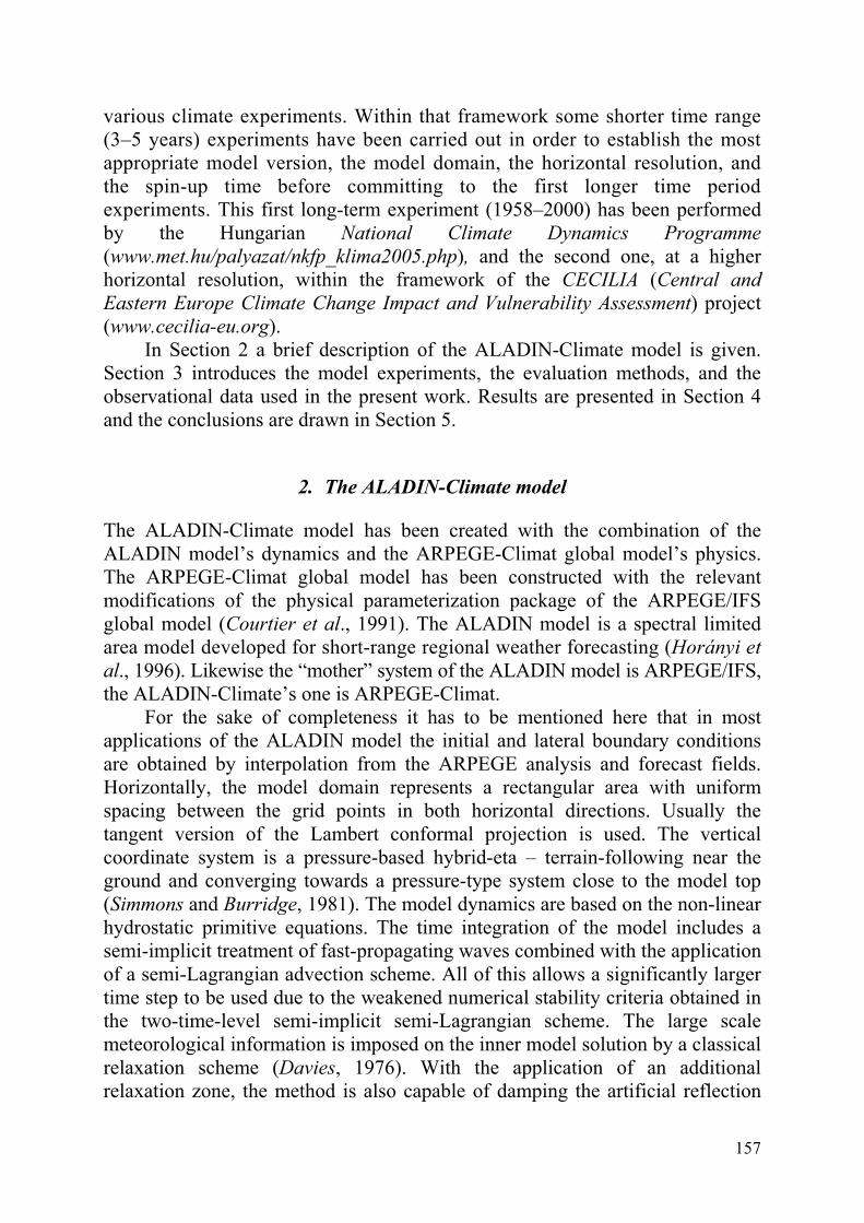
2. The ALADIN-Climate model

The ALADIN-Climate model has been created with the combination of the ALADIN model’s dynamics and the ARPEGE-Climat global model’s physics. The ARPEGE-Climat global model has been constructed with the relevant modifications of the physical parameterization package of the ARPEGE/IFS global model (Courtier et al., 1991). The ALADIN model is a spectral limited area model developed for short-range regional weather forecasting (Horányi et al., 1996). Likewise the “mother” system of the ALADIN model is ARPEGE/IFS, the ALADIN-Climate’s one is ARPEGE-Climat.

For the sake of completeness it has to be mentioned here that in most applications of the ALADIN model the initial and lateral boundary conditions are obtained by interpolation from the ARPEGE analysis and forecast fields. Horizontally, the model domain represents a rectangular area with uniform spacing between the grid points in both horizontal directions. Usually the tangent version of the Lambert conformal projection is used. The vertical coordinate system is a pressure-based hybrid-eta – terrain-following near the ground and converging towards a pressure-type system close to the model top (Simmons and Burridge, 1981). The model dynamics are based on the non-linear hydrostatic primitive equations. The time integration of the model includes a semi-implicit treatment of fast-propagating waves combined with the application of a semi-Lagrangian advection scheme. All of this allows a significantly larger time step to be used due to the weakened numerical stability criteria obtained in the two-time-level semi-implicit semi-Lagrangian scheme. The large scale meteorological information is imposed on the inner model solution by a classical relaxation scheme (Davies, 1976). With the application of an additional relaxation zone, the method is also capable of damping the artificial reflection

158

and transmission of small scale waves on the boundaries of the domain of interest. Model prognostic variables are zonal and meridional wind components, temperature, specific humidity, and surface pressure.

The physical parameterization package of the ALADIN-Climate model largely corresponds to the physics of the ARPEGE-Climat global model. It uses the Fouquart and Morcrette radiation scheme (FMR), which follows the concept of Morcrette (1989) and is based on the ECMWF model including the effects of the greenhouse gases and direct effects of aerosols based on Tegen monthly climatology. As for the land-scheme, the ALADIN-Climate model applies the ISBA (Interaction of Soil Biosphere Atmosphere) scheme (Noilhan and Planton,1989), which involves four soil temperature layers without a deep relaxation, two soil moisture layers, and a single layer snow model with variable albedo and density based on Douville et al. (1995). The deep convection scheme follows Bougeault (1985), but unlike the short range version of the model, it excludes the entrainment and detrainment profiles from the description of convective precipitation processes. Ricard and Royer’s scheme (1993) is used for cloudiness and Smith’s scheme (1990) for large scale precipitation.

3. Experiments and evaluation

The basic objective of the recent work is to understand and assess the behavior of the ALADIN-Climate model regarding its ability to represent the climate of the recent past. Without such thorough testing the model cannot be used for providing climate simulations for the future (although the validation information based on the simulations of the past cannot be directly and explicitly applied for the “bias correction” of the scenario integrations). For this kind of evaluation, the most common approach is to integrate the model over a recent, sufficiently long period (e.g., 40 years) using “perfect” lateral boundary conditions, such as the ERA-40 dataset derived at ECMWF (Uppala et al., 2005). It is noted here that the ERA-40 data are certainly not perfect in every sense – they have their own deficiencies as well (Simmons et al., 2004; Hagemann et al., 2005). However, they do provide one of the best estimates of the past and present climate. Furthermore, during the ERA-40-driven model integrations (due to the differences between the derivation of the ERA-40 data and the internal dynamics and physics of the ALADIN-Climate model) some unbalances might occur, arising from the boundary conditions. Nevertheless, in spite of these deficiencies, the ALADIN-Climate model integration driven by the ERA-40 data is considered to be a reliable solution for the application of the model in reproducing the recent past climate over our domain of interest.

Two model domains and resolutions were defined: a larger domain with 25 km horizontal resolution and a smaller one with 10 km resolution, both with 31 vertical levels. The domains and their orography are shown in Fig. 1. Both

159

domains were used for model integrations between 1958 and 2000, where the first three years were considered as the spin-up period, therefore, the results were evaluated only for the period 1961–2000. The smaller 10 km resolution domain was used to assess the impact of the resolution increase and domain changes as compared to the coarser resolution and larger domain integrations. A third simulation was carried out with the smaller domain for the period of 1960–1990. This integration was driven by the ARPEGE-Climat model. It is noted here that the ARPEGE-Climat boundary conditions are in much better physical and dynamical consistency with the ALADIN-Climate model, than the ERA-40 data. The ARPEGE-Climat model has a variable resolution being around 50 km over Southern Europe, decreasing to 300 km at the antipode (Table 1).

Fig. 1. The ALADIN-Climate model domain and orography for the 25 km (left) and 10 km (right) integrations.

The drawback in applying the ARPEGE-Climat model as lateral boundary condition is that it is also a simulation, which might have biases with respect to the real climate. Therefore, it is worth checking how the “perfect, but inconsistent” and the “simulated, but consistent” boundary conditions compare for the same limited area model integration. Two factors should be kept in mind while considering the length of the spin-up period for the ALADIN-Climate simulations driven by the ARPEGE-Climat model: the global lateral boundary conditions are already in good dynamical and physical balance; and there are similarities (in terms of dynamical core and physical parameterizations) between the global and limited area models. Therefore, the spin-up period for this integration was shorter than was the case for the ERA-40 run. In practice, this means that for the 1960–1990 integrations just the first year was considered as spin-up time and the 1961–1990 classical reference period was used for the evaluation. In spite of the difference in spin-up periods, it is believed that the different model simulations are fully comparable.

160

Table 1. Basic characteristics of the different integrations analyzed

Short name referred to in this paper

Domain Horizontal resolution

(km)

Verticallevels

Timestep(minutes)

Initial and lateral boundaryconditions

ALADERA_25 lat: 35.8 – 59.3ºN lon: 4.8 – 44.1ºE

25 31 15 ERA-40

ALADERA_10 lat: 44.6 – 50.0ºN lon: 12.4 – 25.2ºE

10 31 6 ERA-40

ALADARP lat: 44.6 – 50.0ºN lon: 12.4 – 25.2ºE

10 31 6 ARPEGE-Climat

ARPEGE global model 50 31 30 –

During the evaluation the different integrations are inter-compared to each other and also compared to different observational datasets (Table 2). These observational data comprise both the widely used Climatic Research Unit (CRU) dataset (New et al., 2000; Mitchell and Jones, 2005) and the Hungariangridded dataset (HUGRID). The CRU data (www.cru.uea.ac.uk, produced by the University of East Anglia) were applied at a resolution of 10 arc minutes (CRU10, Mitchell et al., 2004). HUGRID was created at the Hungarian Meteorological Service by the Meteorological Interpolation based on Surface Homogenized Data Basis (MISH) method (Szentimrey et al., 2005), which was developed for the spatial interpolation of different conventional meteorological observations. These data are available for the Hungarian territory with 0.1 degree latitude-longitude resolution.

Table 2. Characteristics of the different observational data used

Domain Resolution

CRU10 lat: 34.0 – 72.0ºN lon: 11.0ºW – 32.0ºE

10 arc minutes

HUGRID lat: 45.7 – 48.6ºN lon: 16.0 – 23.0ºE

0.1 degree

It is important to note that for the production of the ARPEGE-Climat model driving fields for the ALADIN-Climate model, an interpolation has been done from the global resolution to the resolution of the ALADIN-Climate model (10 km). This interpolation is performed on anomaly values, where explicitly the differences between the ARPEGE-Climat model and the surface climatic values (for instance orography, albedo, emissivity, land-sea mask, etc.) of the global model are considered. After interpolation to the target grid (in this case to 10 km), the interpolated anomaly values are added to the higher resolution surface climatic values provided for the regional climate model. Based on this method, the information of the coarse resolution (50 km) global model (projected to the

161

regional one) also reflects high-resolution surface properties, such as higher mountains or the areas around big lakes, for example.

The evaluations are carried out through the assessment of deviations from the observations, and additionally, systematic errors and root mean square errors (RMSE) are computed. With reference to RMSE it is already anticipated here that the RCMs cannot be expected to simulate the time series of annual or seasonal means if the driving data are given by global climate model – and not a re-analysis database – since the global models are unable to provide information on individual years. The global and regional climate models are expected to simulate only the long term inter-annual variability and the average behavior of the climate system on a longer time scale (30 – 40 years). Consequently, it is not expected that results in terms of RMSE, the frequency distributions of the parameters or the temporal evolution charts, would be as good as those from the ERA-40-driven cases. It is also noted that the 2D-map evaluations (patterns) are computed over the domain of the 10 km resolution model, and all the other evaluations (tables, time evolution and frequency distribution figures) are made on the Hungarian territory.

4. Results

4.1. 2m temperature

It can be clearly seen (Fig. 2) that the models have systematic underestimation with respect to the CRU10 dataset. This temperature underestimation is generally 1–3 ºC in the ERA40-driven cases (ALADERA_25 and ALADERA_10) and around 1 ºC in the ARPEGE-driven (ALADARP) case and in the ARPEGE-Climat (ARPEGE) global model itself.

Looking at the results in detail, the simulations are always closer to the observations in the area of the Carpathian Basin – which is a relatively flat terrain – than in the higher mountains. Additionally, for the 10 km simulations the biggest systematic errors arise near to the model boundaries. The errors in the Alpine region are considerable in all simulations. This is attributed not only to the impact of the model boundaries (though the error is largest in the case of the 10 km simulations, where the model boundaries are near to the high mountains) but also to the orography mis-representation within both the models and the observational data sets.

Focusing only on the basin area, particularly over Hungary, the global and the ARPEGE-driven simulations are the closest to the observations – the underestimation remains under 1 ºC over the largest part of the Hungarian territory. On the other hand, slight overestimation seems to occur in the eastern part of the basin, on the Great Hungarian Plain (see Fig. 3, where the eastern part of Hungary is zoomed and another color palette is used). This characteristic feature of the global model, as can be seen later, remains the same in the different

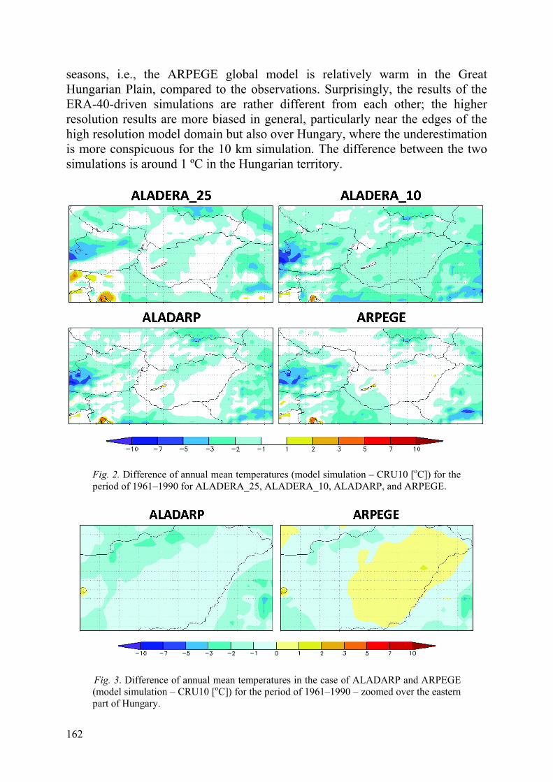
162

seasons, i.e., the ARPEGE global model is relatively warm in the Great Hungarian Plain, compared to the observations. Surprisingly, the results of the ERA-40-driven simulations are rather different from each other; the higher resolution results are more biased in general, particularly near the edges of the high resolution model domain but also over Hungary, where the underestimation is more conspicuous for the 10 km simulation. The difference between the two simulations is around 1 ºC in the Hungarian territory.

Fig. 2. Difference of annual mean temperatures (model simulation – CRU10 [oC]) for the period of 1961–1990 for ALADERA_25, ALADERA_10, ALADARP, and ARPEGE.

Fig. 3. Difference of annual mean temperatures in the case of ALADARP and ARPEGE (model simulation – CRU10 [oC]) for the period of 1961–1990 – zoomed over the eastern part of Hungary.

163

Regarding the seasonal mean temperature difference fields (Fig. 4) in general, the simulations are colder than the observations in the transitional seasons (spring and autumn), and are, with some exceptions, rather near to the observations in summer and winter. The systematic underestimation exceeds 5 ºC in some mountainous regions and even 7–10 ºC in the Alps during the transitional seasons.

Fig. 4. Difference of seasonal mean temperatures (model simulation – CRU10) [oC]) for the period of 1961–1990 (from the top to the bottom: ALADERA_25, ALADERA_10, ALADARP and ARPEGE).

Probably due to the deficiencies of the observation datasets in the high mountains and the negative impact of the model boundaries, as in the annual case, the estimations are always closer to the observations in the fairly flat Carpathian Basin, than in the higher mountainous areas. Moreover, the biggest errors occur again near to the model boundaries in the 10 km simulations. Curiously, in the case of the ARPEGE-Climat global model (which does not suffer from any lateral boundary problem), similar large errors can also be seen at the edges of the 10 km domain, mainly in the high mountains. This is probably due to the inaccurate description of the orography.

Concentrating only on the basin area, all of the simulations give similar results in spring: the underestimation of temperature is higher than the annual systematic error; it is between 1 and 2 ºC on the plains and 2–3 ºC in the hills. The 25 km simulation in autumn shows relatively similar results to spring but, unexpectedly, the 10 km simulations have an even bigger negative bias. These

164

significant underestimations in the transitional seasons cause a slight annual negative bias in the majority of the model versions examined, even if the other seasons show positive biases. The ERA-40 forced versions are fairly unbiased during the summer – the underestimation exceeds 1 ºC only in the Hungarian mountains. However, 1–2 ºC overestimation can be seen in the ARPEGE and ALADARP integrations. Due to this summer overestimation, the ARPEGE-driven case and the global model have smaller annual systematic errors (almost unbiased) than the ERA-40-driven versions. While the ERA-40-driven versions are closer to the observations in summer than in winter, the ALADARP is almost perfectly unbiased in winter, and it has a relatively big overestimation in summer. The disagreement between the ARPEGE-driven ALADIN-Climate model and its driving model is largest in the coldest season. While the regional model has practically no bias, the systematic errors of the ARPEGE-Climat model exceed 2–3 ºC in the eastern part of Hungary. If the difference maps of the ARPEGE-Climat model are studied more carefully, it can be seen that it has relatively large systematic errors throughout the year; however, these biases have different signs (as will be shown later, where the systematic errors are quantified) and compensate for each other during the year resulting in a rather good annual performance (Fig. 2). On the other hand, the “always relatively warmer” Great Hungarian Plain in the driving model decreases the bias of the model over the domain in spring and autumn, and increases it, by about 2–3 ºC,in summer and even more in winter.

The systematic errors given in Table 3 objectively quantify the evaluations based on Figs. 2–4 for the Hungarian area. Annually, the ERA-40-driven model versions have bigger systematic errors than the global and the ARPEGE-driven ones. As mentioned above, the smallest annual bias can be found in the ARPEGE-Climat model. Although it has the coarsest horizontal resolution and the systematic errors are relatively large in every season, the biases with different signs compensate each other. The ERA-40-driven cases are better, particularly during the summer. Surprisingly, the performances of the two ERA-40 simulations are rather different in terms of bias especially in autumn, when the ALADERA_10 simulations are systematically worse than those of the ALADERA_25. The global model has a bias one order of magnitude larger than that of the driven ALADIN-Climate version for winter. As indicated earlier, the global model, throughout the year, simulates the temperature field of the Great Hungarian plain with a much larger warm bias than in other areas of the domain. This is also true when compared to the other model versions. These relatively large positive errors during summer and winter in the eastern part of Hungary cause bigger biases for the ARPEGE than in the case of ALADARP. Though it can be expected that the limited area model improves the simulations of the global model by the coupling, it is not certain that the desired “added value” is the only answer for this significant difference. While the size of the errors is bigger in the transitional seasons in all of the model cases examined, the

165

differences between the simulations are much larger in summer and winter; on the other hand, the models are very close to each other in spring and autumn.

The results of the models compared against CRU10 are similar to those against the Hungarian gridded dataset. The small differences can be explained by the different resolution of the two observational datasets. The differences between the two datasets are particularly emphasized in the mountainous areas, where the temperatures are lower in the HUGRID data. Consequently, when the models have negative systematic errors compared to the CRU10 dataset, the absolute values of the errors are slightly decreased with respect to the HUGRID data.

Table 3. Systematic errors of annual and seasonal simulated temperature fields against the CRU10 and the HUGRID data in the case of ALADERA_25, ALADERA_10, ALADARP, and ARPEGE experiments, in the area of Hungary for the period of 1961–1990

Temperature bias [oC] Annual Spring Summer Autumn Winter

ALADERA_25 – CRU10 –1.05 –1.99 –0.25 –1.61 –0.66 ALADERA_10 – CRU10 –1.50 –2.12 –0.60 –2.66 –0.88 ALADARP – CRU10 –0.80 –2.01 1.06 –2.69 0.11 ARPEGE – CRU10 –0.37 –1.91 1.29 –2.27 1.11

ALADERA_25 – HUGRID –0.89 –1.84 –0.13 –1.14 –0.36 ALADERA_10 – HUGRID –1.41 –2.05 –0.56 –2.28 –0.72 ALADARP – HUGRID –0.72 –1.94 1.10 –2.31 0.27 ARPEGE – HUGRID –0.29 –1.83 1.32 –1.89 1.27

Table 4. Root mean square errors of annual and seasonal simulated temperature fields against the CRU10 and the HUGRID data in the case of ALADERA_25, ALADERA_10, ALADARP, and ARPEGE experiments, in the area of Hungary for the period of 1961–1990

Temperature RMSE [oC] Annual Spring Summer Autumn Winter

ALADERA_25 – CRU10 1.12 2.05 0.80 1.71 1.71 ALADERA_10 – CRU10 1.55 2.17 0.89 2.71 1.26 ALADARP – CRU10 1.15 2.34 1.80 3.22 2.33 ARPEGE – CRU10 1.06 2.26 1.85 2.95 2.74

ALADERA_25 – HU 0.97 1.90 0.78 1.26 1.01 ALADERA_10 – HU 1.46 2.09 0.83 2.33 1.17 ALADARP – HU 1.13 2.31 1.82 2.95 2.37 ARPEGE – HU 1.08 2.23 1.89 2.72 2.82

In order to get a deeper insight into the behavior of the regional climate simulations, it is not sufficient to focus only on the systematic errors, since large errors of opposite sign may compensate each other resulting in a perfectly unbiased – though far from accurate – model. For instance, within the ALADERA_25 and ALADERA_10 simulations, underestimation (negative bias) occurs in every

166

season and, therefore, the annual bias is a relatively large negative value. On the other hand, for ALADARP the bias is changing its sign across the seasons resulting in a smaller annual bias value. Indeed, if the root mean square errors (RMSE, Table 4) are examined, then (for instance) the ALADERA_25 and the ALADARP annual values are rather near to each other, in spite of the fact that the bias characteristics were better for ALADARP.

Fig. 5. Frequency distribution of seasonal temperature differences with respect to CRU10 data for ALADERA_25, ALADERA_10, ALADARP, and ARPEGE simulations. X axis: temperature difference [oC] in the range of [–10, +10]. Y axis: frequency [%] in the range of [0, 50] (gray: positive bias, black: negative bias).

Fig. 5 shows the relative frequency distributions of the seasonal temperature systematic errors, specifically, the distribution of the different amplitudes of the systematic errors, measured year by year and gridpoint by gridpoint in the different seasons. These plots indicate the amount of the positive (gray) and negative (black) biases during the 30 years in the different seasons. For these kinds of diagrams the bias is optimal if the histograms are symmetric around the zero line (the total area of the gray and black columns are the same). In those model cases, where the graph of the distribution function of the frequency is relatively narrow and high, and naturally the peak is not too far from the zero x coordinate, the RMSE is reasonably low. Where the graph is wide and low, even if the area of the positive and negative biases are the same (that is the bias of the whole period is close to zero), the RMSE is considerably high.

167

These kinds of charts are based on the year by year biases. The global model driven cases (and the global models themselves) are not expected to simulate the time evolution of the atmosphere during the examined period (see explanation above). Therefore, unsurprisingly, the range of the differences is much wider in the case of ALADARP and ARPEGE, than that in the ERA-40-driven cases.

Fig. 6. Temporal evolution of the seasonal mean temperature of the examined models and observational data (CRU10: light green; HUGRID: yellow; ALADERA_25: red; ALADERA_10: orange; ALADARP: blue; ARPEGE: purple).

Correspondingly, studying the temporal evolution of the mean temperature during the 30 years examined (Fig. 6), the main variability features for the ERA-40-driven cases (red, orange) are naturally in good agreement with the observations (yellow and green). On the other hand, for the ARPEGE and ARPEGE-driven ALADIN-Climate (purple and blue, respectively) simulations of the variability characteristics can be evaluated only by considering the entire 30 years without any direct links to the individual years. This arises from the fact that only the global external forcing, and not the initial conditions, constrains the limited area model simulation; consequently the climate adaptation process is realized over a longer time scale.

168

For spring and autumn, all models underestimate the temperature in the entire period of 1961–1990. As the average distances between the different models and the observations are comparable, the models have roughly similar bias and RMSE values. On the other hand, while ARPEGE and ALADARP overestimate, the ERA-40-driven simulations underestimate the summer temperature throughout most of the years and, as in the transitional seasons, the model biases have essentially the same sign during the entire period. Therefore, smaller bias seems to indicate smaller RMSE (and vice versa) in all of the seasons except for winter. In the coldest season the ALADARP values are situated randomly under or over the observations, therefore, the systematic error is small in spite of the fact that the difference in errors between individual years can even exceed 5 ºC, providing a large RMSE.

Summarizing the results for the temperature, it can be said that annually and in winter the systematic errors of the ARPEGE-driven ALADIN-Climate model seem to be lower than the reanalysis-driven models’ errors. However, the results are comparable in the transitional seasons, and the ERA-40-driven versions have smaller biases than the other models in summer. As far as the RMSE and the year-by-year variability characteristics are concerned, the correlation between the ERA-40-driven cases and the observed data are obviously higher than is the case between the observations and ARPEGE or ALADARP. This fact corresponds to our initial expectations, indicating that the global model and the limited area model driven by the global one are unable to simulate the time series of annual or seasonal means. Subsequently, the frequency distributions are reasonably high and narrow in the cases of the ERA-40-driven simulations (low RMSE), and rather low and wide in the case of the ARPEGE and ALADARP ones (high RMSE).

4.2. Precipitation

From hereinafter only the ALADERA_25, ALADERA_10, and ALADARP simulations are evaluated.

Looking at the annual relative differences (the deviations between the simulations and the observations normalized by the corresponding values of the observational data), generally a 10–50% overestimation can be seen in the Carpathian Basin for all of the models investigated (Fig. 7). The systematic errors are much larger outside the basin, especially for the ALADERA_10 simulation. There is also an underestimation pattern appearing in the south-western part of the domain for every experiment, which is more pronounced within the high resolution model versions. The biggest errors are near to the model boundaries indicating spurious precipitation patterns originating from the lateral boundaries: it is especially true for the two 10 km integrations. Moreover, the lower resolution ALADIN-Climate model, due to the smaller biases at the edges of the visualization domain (which are not the physical boundaries in that

169

case), has the smallest spatial variability in terms of model bias. The best simulation for the Carpathian Basin is the ARPEGE-driven one, which obviously indicates the importance of the proper dynamical and physical balance between the coupling and coupled models. The systematic error in the southwest part of Hungary is around zero, and basically, with some small exceptions, the errors remain under 30% throughout Hungary. A patchy picture can be seen in the results of ALADERA_25, which shows slightly worse results than ALADARP, but considerably better than the high resolution ERA-40-driven run. Although the largest systematic errors can be seen in the ALADERA_10 simulation, the errors are rather small in the southwest part of the Carpathian Basin. All of this means that the resolution increase for the ERA-40-driven models does not automatically improve the performance of the simulation. It might be attributed to the difference between the resolutions of the driving and the driven models. The increase in resolution is causing more discrepancy through the lateral boundaries and furthermore the proximity of the boundaries (which are situated over mountainous regions), which might cause unrealistic precipitation fields near to them.

Fig. 7. Relative difference of annual mean precipitation for the period of 1961–1990 for ALADERA_25, ALADERA_10, and ALADARP (model simulation – CRU10)/CRU10 [%]).

Regarding the seasonal features in general, spring and summer are more humid than the observations in all of the simulations, and a relatively variable pattern with locally significant over- and underestimations can be seen during

170

autumn and winter. While the relative difference of precipitation is around zero in winter in the Carpathian Basin, very extreme positive and negative values can be seen outside the basin, near the model boundaries. The autumn features are extremely different and the best results (as for the annual situation) are in the low resolution model case. The ALADERA_10 and ALADARP simulations are rather similar, except for summer, when the ARPEGE-driven integration performs significantly better than the ERA-40-driven one. It can also be seen that all of the models (even ALADERA_25) have very variable results outside the Carpathian Basin. Inside the Basin, all simulations give similar results in spring with a general significant overestimation pattern. This positive bias is also typical for the summer for all of the models. However, there is a significant difference between the worst version (ALADERA_10) and the best one (ALADARP). During the autumn very low bias (overestimation) can be seen in the Carpathian Basin in the 25 km resolution ERA-40-driven model. The other two models have larger negative systematic errors all across the domain. Regarding the winter season, while the ALADERA_25 results are rather similar to its autumn ones, the maps of the ALADERA_10 and ALADARP models have very different features. While the models underestimate the precipitation in the southwest and overestimate it along the other parts of the domain edges, the bias in the majority part of Hungary remains reasonably good. The biggest differences between the two model results are the (positive) extremes in the eastern part of the domain.

As far as the bias values are concerned, Table 5 reflects the Hungarian situation as can be also derived from Figs. 7 and 8. These values help to quantify those small differences, which are otherwise difficult to interpret subjectively.

Table 5. Systematic errors of annual and seasonal simulated precipitation fields against the CRU10 and the HUGRID data in the case of ALADERA_25, ALADERA_10, and ALADARP experiments in the area of Hungary for the period of 1961–1990

Precipitation bias [mm/months] Annual Spring Summer Autumn Winter

ALADERA_25 – CRU10 15.31 31.11 22.06 3.56 4.50 ALADERA_10 – CRU10 18.72 33.36 49.91 –8.53 0.14 ALADARP – CRU10 9.33 31.72 15.12 –10.20 0.83

ALADERA_25 – HUGRID 15.60 30.34 23.35 4.76 4.55 ALADERA_10 – HUGRID 18.69 32.14 50.96 –7.43 –0.26 ALADARP – HUGRID 9.30 30.49 16.17 –9.11 0.44

Taking into account the fact that the global models and the global model driven simulations are able to simulate only the long term inter-annual variability, as in the case of temperature, a short review of the results of the RMSE, the frequency distribution and temporal evolution charts of precipitation is given below.

171

Fig. 8. Relative difference of seasonal mean precipitation for the period of 1961–1990 (model simulation – CRU10)/CRU10 [%]) (from top to the bottom: ALADERA_25, ALADERA_10, and ALADARP, respectively).

Table 6. Root mean square errors of annual and seasonal precipitation against the CRU10 and the HUGRID data in the case of ALADERA_25, ALADERA_10, and ALADARP experiments in the area of Hungary for the period of 1961–1990

Precipitation RMSE [mm/months] Annual Spring Summer Autumn Winter

ALADERA_25 – CRU10 18.00 34.23 30.80 13.54 9.99 ALADERA_10 – CRU10 20.91 35.61 54.10 14.72 11.22 ALADARP – CRU10 15.58 37.12 35.58 22.09 18.25

ALADERA_25 – HUGRID 18.54 33.91 32.23 14.05 10.65 ALADERA_10 – HUGRID 21.19 34.68 55.57 14.81 12.78 ALADARP – HUGRID 16.39 36.36 37.04 22.75 19.89

As already explained and demonstrated for temperature, the small bias may not indicate small RMSE values due to the possible cancellation effects arising from the bias computations. In order to illustrate this feature for precipitation as well, the winter values of ALADARP and ALADERA_25 are considered. While the ALADARP experiment possesses a rather small bias value (0.83), the ALADERA_25 is characterized by a larger one (4.5). On the other hand the RMSE of ALADERA_25 is significantly lower (9.99) than in the case of ALADARP (18.25). Essentially, small bias corresponds to large RMSE (Table 6)and vice versa. That is because the ALADERA_25 integration has significant systematic overestimation – which is present for a large part of the domain in the majority of the years and in basically all the seasons –, but it does not manifest

172

itself in big RMSE values because the overestimation values are not too big. In contrast, ALADARP results have very small systematic error, but significant RMSE values, at the same time, because there are significant errors of different signs across the domain and throughout the different seasons during the period studied.

Fig. 9. The frequency distribution of seasonal precipitation differences with respect to CRU10 data for ALADERA_25, ALADERA_10 and ALADARP. X axis: difference of precipitation [mm] in the range of [–150, +150 ]. Y axis: frequency [%] in the range of [0, 30] (black: negative bias, gray: positive bias).

The same issue can be also seen, while looking at the frequency distribution of seasonal precipitation differences (Fig. 9). The two histograms for ALADERA_25 and ALADARP in winter are rather different: narrow, high, and asymmetric for ALADERA_25 and lower, wider, and more symmetric for ALADARP. There is an annual variation of the frequency distribution in every experiment; the histograms are relatively high and narrow in winter and low and wide in summer. This fact confirms that the general predictability of precipitation is much higher in winter than in summer. Although, the histogram of ALADARP is slightly lower and wider than the ALADERA_10’s one in the warmest season, its RMSE remains smaller than that of the ALADERA_10. This is because the systematic errors of ALADARP are around zero and the errors are not extremely big, and in the case of ALADERA_10 the absolute errors are rather high and they are mostly realized in overestimations.

Regarding the seasonal mean precipitation variation (Fig. 10), it can be seen that, as expected, the two kinds of observations (CRU10 and HUGRID in green and yellow) run together. Also the trends of the ERA-40-driven cases (red, orange) are similar to the observational ones. Particularly, the maximum and minimum values are roughly at the same places, although the correlation,

173

particularly during summer, is not as good as was the case for temperature. As ALADARP cannot represent the observed series of year (see Sect. 3), the behavior of the ALADARP simulation (blue) is rather different to the ERA-40- driven cases. During spring, all models overestimate the precipitation for every year of the period 1961–1990. For summer, the picture is more chaotic: the high resolution ERA-40-driven results are relatively far from the observations, while the lower resolution version is closer to reality. Nevertheless, the two curves are still basically parallel. In autumn the ERA-40-driven versions have some bias – the low resolution model overestimates and the high resolution one underestimates the precipitation. However, the differences are smaller than in spring and summer, hence the RMSE and bias values are lower. The correspondence between the different experiments and the observations is best during winter. This fact is also apparent on the rather high and narrow (i.e. small errors) distribution functions in that season (Fig. 9).

Fig. 10. The temporal evolution of the seasonal mean precipitation of the examined models and observational data (CRU10: light green; HUGRID: yellow; ALADERA_25: red; ALADERA_10: orange; ALADARP: blue).

In summary, the results of the simulated precipitation over the Carpathian Basin show that ALADARP is the best annually and in the extreme seasons. Regarding the RMSE and the inter-annual characteristics, the correlation

174

between the ERA-40-driven cases and the observed data is unsurprisingly higher than is the case for the ARPEGE-driven simulation. On the other hand, the low resolution ERA-40-driven case (ALADERA_25) has better verification characteristics than that of the high resolution re-analysis-driven case (ALADERA_10).

5. Conclusions

The aim of this paper was to give a comprehensive analysis of temperature and precipitation fields of the ALADIN-Climate model “family” integrated at the Hungarian Meteorological Service. Four different kinds of simulation have been investigated in the case of temperature, and three in the case of precipitation. These simulations are the 25 km resolution ALADIN-Climate (LBC: ERA-40), the 10 km resolution ALADIN-Climate (LBC: ERA-40), the 10 km resolution ALADIN-Climate (LBC: ARPEGE-Climat) and, only in the case of temperature, the ARPEGE-Climat model. It was considered essential to explore the behavior of the available climate models for the recent past, since valuable information can be expected from the simulations of the future only if the main characteristics of the models are well known and its strengths and weaknesses are explored. This statement is true in spite of the well-known fact that the error characteristics for the past might not have any relation with those for the scenario runs. Moreover, it is also generally accepted that changes in the future are computed with respect to the same model simulations for the past. This technique implicitly assumes that the same error characteristics occur in the past as for the future (this fact cannot be verified and most probably is not true), hence the difference between the absolute fields automatically neglects those errors.

It was largely illustrated that the global climate models, and those regional climate models that are driven by global models, are not expected to simulate the time series of annual or seasonal means (only the long term inter-annual variability), since the global models do not provide any information on real years. Nevertheless, it is expected from all of the model versions that the average behavior of the atmosphere is reasonably well simulated for a longer time period (typically 30 years).

The figures and tables in this paper illustrated that the ARPEGE-driven version and even the driving model, in general, give better results in the Carpathian Basin for the whole period (1961–1990), than the ERA-40-driven versions. These results are certainly due to the much better physical and dynamical consistency between the ALADIN-Climate and ARPEGE-Climat models than between the limited area model and the ERA-40 data. Moreover, the coupled ALADARP gives better results than its mother model (the ARPEGE-Climat global model), providing the anticipated “added value” by the application of the higher resolution regional climate model.

175

The examination and comparison of the two “observation-driven” cases helps to draw some conclusions about the sensitivity of the simulations with respect to the domain size and resolution. The realization, that the lower resolution model (in a bigger domain) gives better results than the higher resolution one (in a smaller domain), points to the fact that the domain of the 10 km resolution model is too small, and the errors appearing at the edges of the model domain have a strong effect on the simulation of the inner area as well.

Finally, based on all of these results, we are tempted to conclude that the results of the ARPEGE-driven regional model – even in this small domain – might be used for making reasonably good projections for the future. If this “climate shift” or “climate transformation” of the investigated regional model is fairly comparable to other models known from different projects (e.g., ENSEMBLES (ensembles-eu.metoffice.com), PRUDENCE (prudence.dmi.dk),etc.) in low resolution, then this provides some reassurance that the model examined will probably provide reliable results and can be used in the future at higher resolution as well.

The future work will concentrate both on the issue of the optimal domain size and resolution for the Central-European climate simulations and on the scenario runs together with their evaluations for the determination of climate scenarios for the Hungarian territory.

Acknowledgements—The authors are very grateful to all of the colleagues of the international ALADIN cooperation for the development of the ALADIN model. Special thanks are given to MichelDéqué and Samuel Somot for their constant support and guidance, while adapting the ALADIN-Climate model and later for answering questions during the experimentation. The fruitful discussions with the members of the Division for Numerical Modeling and Climate Dynamics of the Hungarian Meteorological Service and all of their valuable help are highly appreciated. The adaptation and first experiments with the ALADIN-Climate model in Hungary were undertaken by Helga Tóth and Andrea L rincz: the authors are indebted to them for all of their work related to the ALADIN-Climate model. Many thanks for Gábor Radnóti for useful comments on parts of the manuscript, which helped significantly on the general understanding of the capabilities of the regional climate models. Special thanks are due for the careful revision work of Tamás Práger, which significantly contributed to the improvements of the manuscript. The other reviewer’s comments were also appreciated and helped while revising the paper. Many thanks for Karl Kitchen for the significant improvement of the English of the manuscript. This work was supported by the European Commission's 6th Framework Programme in the framework of CECILIA project (contract number 037005), the Hungarian National Office for Research and Technology (NKFP, grant No. 3A/082/2004), and the János Bolyai Research Scholarship of the Hungarian Academy of Science.

References

Bougeault, P., 1985: A simple parameterization of the large-scale effects of cumulus convection. Mon. Weather Rev. 113, 2108-2121.

Brankovic, T. and Gregory, D., 2001: Impact of horizontal resolution on seasonal integrations. Clim.Dynam. 18, 123-143.

Coppola, E. and Giorgi, G., 2005: Climate change in tropical regions from high-resolution time slice AGCM experiments. Q. J. Roy. Meteor. Soc. 131, 3123-3145.

176

Courtier, Ph., Freydier, C., Geleyn, J.-F., Rabier, F., and Rochas, M., 1991: The ARPEGE project at Météo-France. In Proc. ECMWF Workshop on Numerical Methods in Atmospheric Modelling.9-13 Sept 1991. Vol. 2, 193-231.

Davies, H.C., 1976: A lateral boundary formulation for multi level prediction models. Q. J. Roy. Meteor. Soc.102, 405-418.

Douville, H., Royer, J.-F., and Mahfouf, J.-F., 1995: A new snow parametrization for the Météo-France climate model. Part I: Validation in stand-alone experiments. Clim. Dynam. 12, 21-35.

Duffy, P.B., Govindasamy, B., Iorio, J.P., Milovich, J., Sperber, K.R., Taylor, K.E., Wehner, M.F., and Thompson S.L., 2003: High-resolution simulations of global climate. Part 1: Present climate. Clim. Dynam. 21, 371-390.

Giorgi, F. and Mearns, L.O., 1991: Approaches to regional climate change simulation: A review. Rev.Geophys. 29, 191-216.

Giorgi, F. and Mearns, L.O., 1999: Introduction to special section: Regional climate modelling revisited. J. Geophys. Res. 104 (D6), 6335-6352.

Hagemann, S., Arpe, L., and Bengtsson, L., 2005: Validation of the hydrological cycle of ERA40. ERA-40 Project Report Series, 24, Reading, UK.

Hewitson, B.C. and Crane, R.G., 1996: Climate downscaling: Techniques and application. ClimateRes. 7, 85-95.

Horányi, A., Ihász I., and Radnóti, G., 1996: ARPEGE/ALADIN: A numerical weather predicition model for Central-Europe with the participation of the Hungarian Meteorological Service. Id járás 100, 277-300.

Horányi A., S. Kertész, L. Kullmann, and G. Radnóti, 2006: The ARPEGE/ALADIN mesoscale numerical modeling system and its application at the Hungarian Meteorological Service. Id járás 110, 203-227.

Janisková, M., 1994: Study of the systematic errors in ALADIN associated to the physical part of the model. Note ALADIN n°7, CNRM, Météo-France, 82 pp.

Kattenberg, A., Giorgi, F., Grassl, H., Meehl, G.A., Mitchell, J.F.B., Stouffer, R.J., Tokioka, T., Weaver, A.J., and Mitchell, T.M.L., 1996: Climate Models. Projections of future climate. In Climate Change 1995: The science of climate change. Second assessment report of the IPCC: Contribution of WG1 (eds.: J.F. Houghton, G. Meira, B.A. Callander, N. Harris, A. Kattenberg, K. Maskell). Cambridge University Press, 285-357.

McGregor, J.L., 1997: Regional climate modelling. Meteorol. Atmos. Phys. 63, 105-117. Mitchell, T.D., Carter, T.R., Jones, P.D., Hulme, M., and New, M., 2004: A comprehensive set of high-

resolution grids of monthly climate for Europe and the globe: the observed record (1901-2000) and 16 scenarios (2001-2100). Working Paper 55. Tyndall Centre for Climate Change Research, University of East Anglia, Norwich, UK.

Mitchell, T.D. and Jones, P.D., 2005: An improved method of constructing a database of monthly climate observations and associated high-resolution grids. Int. J. Climatol. 25, 693-712.

May, W. and Roeckner, E., 2001: A time-slice experiment with the ECHAM4 AGCM at high resolution: The impact of horizontal resolution on annual mean climate change. Clim. Dynam.17, 407-420.

Morcrette, J.-J., 1989: Description of the Radiation Scheme in the ECMWF Model. Technical Memorandum, 165, ECMWF, 26 pp.

New, M., Hulme, M., and Jones, P.D., 2000: Representing twentieth century space-time climate variability. Part 2: development of 1901–96 monthly grids of terrestrial surface climate. J. Clim.13, 2217-2238.

Noilhan, J. and Planton, S., 1989: A simple parametrization of land surface processes for meteorological models’. Mon. Weather Rev. 117, 536-549.

Ricard, J.-L. and Royer, J.-F., 1993: A statistical cloud scheme for use in a AGCM. Ann. Geophysicae11, 1095-1115.

Simmons, A.J. and Burridge, D.M., 1981: An energy and angular-momentum conserving finite-difference scheme and hybrid vertical coordinates. Mon. Weaather Rev. 109, 758-766.

Simmons, A.J., Jones, P.D., and da Costa Bechtold, V., 2004: Comparison of trends and variability in CRU, ERA-40 and NCEP/NCAR analysis of monthly-mean surface air temperatures. ERA-40Project Report Series 18. Reading, UK, ECMWF Re-Analysis Project. 38p.

177

Smith, R.N.B., 1990: A scheme for predicting layer clouds and their water content in a general circulation model. Q. J. Roy. Meteor. Soc. 116, 435-460.

Szentimrey, T., Bihari, Z., and Szalai, S., 2005: Meteorological Interpolation based on Surface Homogenized Data Basis (MISH). Geophys. Res. Abstracts 7, 2005.

Uppala, S.M., Kållberg, P.W., Simmons, A.J., Andrae, U., da Costa Bechtold, V., Fiorino, M., Gibson, J.K., Haseler, J., Hernandez, A., Kelly, G.A., Li, X., Onogi, K., Saarinen, S., Sokka, N., Allan, R.P., Andersson, E., Arpe, K., Balmaseda, M.A., Beljaars, A.C.M., van de Berg, L., Bidlot, J., Bormann, N., Caires, S., Chevallier, F., Dethof, A., Dragosavac, M., Fisher, M., Fuentes, M., Hagemann, S., Hólm, E., Hoskins, B.J., Isaksen, L., Janssen, P.A.E.M., Jenne, R., McNally, A.P., Mahfouf, J.-F., Morcrette, J.-J., Rayner, N.A., Saunders, R.W., Simon, P., Sterl, A., Trenberth, K.E., Untch, A., Vasiljevic, D., Viterbo, P., and Woollen, J., 2005: The ERA-40 re-analysis. Q. J. Roy. Meteor. Soc. 131, 2961-3012.

Wang, Y., Leung, L.R., McGregor, J.L., Lee, D.K., Wang, W.C., Ding, Y., and Kimura, F., 2004: Regional climate modeling: Progress, challenges, and prospects. J. Meteor. Soc. Japan 82,1599-1628.

Wilby, R.L., Charles, S.P., Zorita, E., Timbal, B., Whetton, P., and Mearns, L.O., 2004: Guidelines for Use of Climate Scenarios Developed from Statistical Downscaling Methods. IPCC Data Distribution Centre, University of East Anglia, U.K., 27pp.