uva-dare (digital academic repository) quantum · pdf file5.2 quantuentanglemenm 8t 3...
TRANSCRIPT

UvA-DARE is a service provided by the library of the University of Amsterdam (http://dare.uva.nl)
UvA-DARE (Digital Academic Repository)
Quantum Algorithms and Quantum Entanglement
Terhal, B.M.
Link to publication
Citation for published version (APA):Terhal, B. M. (1999). Quantum Algorithms and Quantum Entanglement
General rightsIt is not permitted to download or to forward/distribute the text or part of it without the consent of the author(s) and/or copyright holder(s),other than for strictly personal, individual use, unless the work is under an open content license (like Creative Commons).
Disclaimer/Complaints regulationsIf you believe that digital publication of certain material infringes any of your rights or (privacy) interests, please let the Library know, statingyour reasons. In case of a legitimate complaint, the Library will make the material inaccessible and/or remove it from the website. Please Askthe Library: http://uba.uva.nl/en/contact, or a letter to: Library of the University of Amsterdam, Secretariat, Singel 425, 1012 WP Amsterdam,The Netherlands. You will be contacted as soon as possible.
Download date: 09 May 2018

Chapter 5
Product Bases, Local Distinguishability
and Bound Entanglement
5.1 Introduction
In this chapter we study fundamental properties of quantum mechanical states, operations
and measurements. In section 5.2 we review the notions of entanglement, distillation of
entanglement and its relation to positive linear maps. In section 5.3 we establish a relation
between Bell inequalities and the separability criterion and show under what restrictions they
are equivalent. In section 5.4 we present results that relate local distinguishability of sets
of product states to bound entanglement. Central in this construction is the notion of an
unextendible product basis, of which we will give many examples. We prove that uncompletable
product bases cannot be distinguished by a finite number of local operations and classical
communication. These uncompletable product bases form new examples of the phenomenon
of nonlocality without entanglement. In section 5.5 we present a new family of indecomposable
positive linear maps. In the following sections we use the notation n ® m or Hn <g> ~Km to
denote the tensorproduct between a n-dimensional Hubert space and a m-dimensional Hubert
space.
5.2 Quantum Entanglement
The study of entanglement is essential for the understanding of quantum mechanics and the use
of quantum mechanics in computation and information processing tasks. Erwin Schrödinger
introduced the notion of entanglement and he was the first to understand its fundamental
importance; in Ref. [105] we find
"When two systems, of which we know the states by their respective repre
sentatives, enter into temporary physical interaction due to known forces between
them, and when after a time of mutual influence the systems separate again, then
they can no longer be described in the same way as before, viz. by endowing each
82 5 PBs, LO+CC and BE
of them with a representative of its own. I would not call that one but rather the
characteristic trait of quantum mechanics, the one that enforces its entire depar
ture from classical lines of thought. By the interaction the two representatives (or
tp-functions) have become entangled."
The simplest form of entanglement is the entanglement that we find in bipartite pure
states. Let \ip) e%A® MB- We call the state \tp) entangled iff \ip) cannot be written as a
product of pure states:
\1>)*\1>*)®\ih), (5.2.1)
where \ipa) e HA and \-ipi,) G HB- Equivalently, when we express the pure state \ip) as a
density matrix \ip)(ijj\, the density matrix is entangled iff it cannot be written as
ww^mm®\^)(M (5.2.2)
The famous example of a bipartite entangled state in 2 ® 2 is the Einstein-Podolsky-Rosen
(EPR) singlet state [106, 107]
|*-> = -^( |01)- |10». (5.2.3)
We are not only concerned with pure states, but also with mixed states, represented by
positive semidefinite Hermitian matrices p with T r p = 1, the density matrices. Let us give
the definition of entanglement for a bipartite density matrix p:
Definition 3 Let p be a density matrix on a finite-dimensional Hilbert space HA ® HB- A
state \ip) of the form \ipA) ® \i^B) is a (pure) product state in HA®HB- The density matrix p
is entangled iff p cannot be written as a convex combination of pure product states, i.e. there
does not exist an ensemble {pi > 0, \ipf ® tpf)} such that
P = Y,P> I ^X^ I ® iVf >0/f I- (5.2.4) i
When p is not entangled p is called separable.
One would also like to classify entanglement in multipartite systems. A famous example
of a tripartite pure entangled state is the Greenberger-Horne-Zeilinger (GHZ) state:
|GHZ) =-^=(|000) + |111)). (5.2.5)
The state cannot be written as a product of three single party states, nor as a product
of an entangled two party and a single party state. The example illustrates that in a full
characterization of the entanglement of multipartite systems we will have specify between
which parties the entanglement occurs. When we look at multipartite density matrices, this
can lead to surprising results. In section 5.4.3 we will give an example (Example 3) of a

5.2 Quantum Entanglement 83
tripartite density matrix which cannot be written as a convex combination of pure product
states for all three parties. When viewed as a bipartite density matrix on HAB ® Hc or
HA ® HBC or HAC ® HB, it can be shown that the density matrix is separable. This is
impossible if the density matrix is a pure state, but apparently allowed when we consider
general density matrices.
5.2.1 Quantification of Entanglement
It is important to have a measure of entanglement that quantifies 'how much entanglement'
a state contains. Here we will only consider a measure of entanglement for bipartite states.
For multipartite states the measure of entanglement has to take into account between which
subsystems the entanglement occurs. It is an open problem how to define a measure of mul
tipartite entanglement that gives a complete description of the various kinds of entanglement
that are present in the state.
Any measure of entanglement E(p) where p is a density matrix on HA ® HB must have
the following four natural properties [37, 108]:
1- E(p) > 0 for all density matrices p and E(p) = 0 when p is a separable density matrix.
2. E(p) is invariant under local unitary transformations, that is, unitary transformations of
the form U = UA®UB-
3. The entanglement E(p) cannot increase under local operations and classical communi
cation, that is
E(S(p)) < E(p), (5.2.6)
where S is a superoperator that can be implemented with local quantum operations of
the two parties A and B and an unlimited amount of classical communication between
them.
4. The entanglement E(p) is a convex function of p, i.e.
E(p=^2lHPi)<^2piE{pi). (5.2.7) i i
For pure states \ip) the conventional measure that obeys the four requirements is the
entropy of entanglement. It is defined as
E(\xb)(ib\) = S(TrA\tl>){4,\) = SCIYBIVXV- I ) , (5.2.8)
where 5 is the von Neumann entropy:
5(p) = -Trplogp. (5.2.9)
84 5 PBs, LO+CC and BE
With this measure the EPR singlet in Eq. (5.2.3) has an entanglement of 1 bit, which is
the maximum for a state in 2 ® 2. For mixed states several entanglement measures have
been proposed. One favorite measure that was introduced in Ref. [37] that obeys all the
requirements is the entanglement of formation. The entanglement of formation for bipartite
mixed states is more complicated than for pure states as the decomposition of a mixed state
into a convex combination of pure states is not unique. Let p be a bipartite density matrix
and let £p = {pi > 0, \ipi)} be an ensemble into which p can be decomposed:
P = Çft |&)(lfe| . (5.2.10) i
The entanglement of formation of p is defined as
E(p) = min V P l £ ( | ^ ) < ^ | ) . (5.2.11) i
The entanglement of formation equals the minimal average amount of pure state entanglement
that is needed to build the density matrix p. The minimization in Eq. (5.2.11) makes an
analytical computation of the entanglement of formation of mixed states a nontrivial task.
Only in 2 ® 2 has the problem of determining the entanglement of formation of any density
matrix been completely solved by Wootters [109].
One may require that a measure of entanglement has the additional property of additivity,
which does not follow from properties 1-4. An entanglement measure E for bipartite states
is additive when for any two density matrices p\ on HAl <g> HBl and p2 on %A2 ® 7iBl and
p = P\ ® pi on HA ® 'HB where %A = HAl ® 'HA2 and 'RB = 7iBl ® 7{B2, the following
holds:
E{p1®p2) = E{pl) + E{p2). (5.2.12)
The entanglement of formation is certainly subadditive
E{pi®p2)<E(Pl)+E{p2), (5.2.13)
where the equality holds when one uses the optimal individual ensembles £Pl and £P2 in the
decomposition of pi ® p2. The entanglement for pure states can be shown to be additive,
but it has not yet been proved that the entanglement of formation is additive for all density
matrices. If the entanglement of formation were not additive then this would mean that the
entanglement costs for making px ® p2 would be strictly less than the entanglement costs for
making p\ and p2 separately. It is possible that the entanglement of formation obeys only the
requirement of partial additivity, that is, for all n= 1 ,2 , . . . E(p®n) = nE(p) for mixed states
p [108].
5.2.2 Disti l lat ion of Quantum Entanglement
The sharing of quantum entanglement between two or more parties is a resource that for
many quantum information processing tasks is more powerful than the sharing of classically
5.2 Quantum Entanglement 85
correlated states. As mentioned in Chap. 1 section 1.2.3, an EPR state can be used to send
quantum information via teleportation. The protocols that employ quantum communication to
solve a classical communication complexity problem (sec. 1.2.2) can be replaced by protocols
that start from sharing a set of entangled states, which are then used to teleport the quantum
data. If in these protocols the two parties start out with a mixed entangled state, they will
have to "purify" this state to a pure entangled state before using it in some protocol. This
procedure is called distillation [36]. The allowed set of quantum operations in the distillation
procedure is restricted to the class of superoperators that is implementable by local quantum
operations (LO) and classical communication (CC). Let us give the definition of distillable
entanglement:
Definition 4 [37, 110] The distillable entanglement of a bipartite density matrix p on H.A®'HB
with an unlimited amount of local operations and an unlimited amount of classical communi
cation (LO+CC) is the maximum number D(p) such that there exists a sequence of LO+CC
T C P maps Si
S, : B{(HA ® UBD -> B{Ki ® /Q), (5.2.14)
with rii —> oo,
— log dim/C,;->£>(/>), (5.2.15) Tli
and fidelity with respect to a maximally entangled state
( $ + | £ ( p ® , l i ) | $ + ) - H ) (5.2.16)
where
p59"' = p(g> ...®p, (5.2.17)
and
l*+) = ^ g l « > - (5Z18) A density matrix p is called distillable if we can distill a non-zero amount of maximally
entangled states from an arbitrary number of copies of p.
In words, this definition says that a density matrix p is distillable by LO+CC if, when given
a large number of copies of the density matrix p, there is a LO+CC procedure that maps these
copies onto a set of states in a (smaller) Hubert space K{ ® K.t such that these remaining
(distilled) states have a high fidelity with respect to a maximally entangled state-for example
the state |$+) - in /Q <g> /C,. Note that we call a density matrix p distillable when some pure
state entanglement can be distilled from it. If only a constant number of maximally entangled

86 5 PBs, LO+CC and BE
states can be distilled from an infinite number of copies of p, then D(p) = 0. We call such a
density matrix distillable though. From property 3, Eq. (5.2.6), it follows that D(p) < E(p);
if D(p) would exceed E(p), we would have increased E(p) by LO+CC.
It has been shown [111] that any entangled density matrix on 2 ® 2 is distillable, in fact it
was found that D(p) > 0 for all entangled density matrices on 2® 2. In higher dimensions the
problem of distillation has turned out to be complicated by the richer structure of the manifold
of entangled states and their relation to positive linear maps.
5.2.3 Positive Linear Maps
The problem of deciding whether a bipartite density matrix p on 'HA®'HB is entangled can be
quite hard. It has been shown by the Horodeckis [112] that there exist an intimate connection
between the classification of entangled density matrices and the theory of positive linear maps.
Let S: B(H„) ->• BCHm) be a linear map. S is positive when S: B(Hn)+ -> B(Hm) +,
where B(H„) + denotes the set of positive semidefinite matrices on 7in. Let idfc be the identity
map on B(Hk). We define the map id* ®<S: B(Hk<Si'Hn) -» B(nk<S>'Hm) for k = 1 ,2 , . . .
by
(id*® S) lj2ai®Ti) =X^®<S(T ')> (5.2.19)
where <7; G B(Hk) and r, e B(Hn). The map S is /c-positive when id* ® S is positive. The
map S is completely positive when S is /c-positive for all k = 1 ,2 , . . . . Following Lindblad
[113], the set of physical operations on a density matrix p e B(7in) + is given by the set of
completely positive trace-preserving maps S: B(Hn) —> B(Hm). Similarly as fc-positive, one
can define a /c-copositive map. Let T: BCHn) -> B(Hn) be defined as matrix transposition
in a chosen basis for "Hn, i.e.
{T{A))n = Aji, (5.2.20)
on a matrix A e B(7in). The map <S is fc-copositive when id * ® (.SoT) is positive. A positive
linear map S : B(Hn) —*• £ (%„ , ) is decomposable if it can be written as
S = S1+S2oT, (5.2.21)
where <Si : B{Hn) ->• B(Hm) and <S2: B(Hn) -» B(7im) are completely positive maps. It
has been shown by Woronowicz [114] that all positive linear maps S: B(%2) -> B{T-L2) and
<S: B(U2) -»• B{H3) are decomposable.
In Ref. [115] Peres made the observation that every separable density matrix p G B(HA <g>
HB) remains positive semidefinite under partial transposition of p, (idA ® Tß)(p). He conjec
tured that this would not only be a necessary but also a sufficient condition for separability.
His conjecture turned out to be true for density matrices on 2 ® 2 and 2 ® 3.
The following theorem by the Horodeckis [112] formulates a necessary and sufficient con
dition for a density matrix p to be entangled:
5.3 Bell Inequalities and the Separability Criterion 87
Theorem 1 (Horodecki) A density matrix p on HA ® HB is entangled iff there exists a
positive linear map S: B(HB) —> B(HA) such that
(idA ®S)(p), (5.2.22)
is not positive semidefinite. Here i d ^ denotes the identity map on B(HA)-
Remark An equivalent statement as Theorem 1 holds for positive linear maps
S: B(HA) —> B(HB) and the positive semidefiniteness of (<S <g> idß)(p).
The consequences of Theorem 1 and Woronowicz' result is that a bipartite density matrix p
on H2®H2 and %2®%3 is entangled iff ( i d^ ® [Si + S2 o T | ) (p) is not positive semidefinite
for some Si and <S2- As Si and S2 are completely positive maps this is equivalent to testing
whether the requirement that (id/i ® T) (p) is not positive semidefinite is satisfied.
In the following sections we will sometimes refer to a density matrix having the NPT-
property, which means that the density matrix is not positive semidefinite under partial trans
position, or a density matrix having the PPT-property.
The partial transposition map is a powerful tool in characterizing entanglement, even in
high dimensional Hilbert spaces. In Ref. [116] it was shown that if a bipartite density matrix p
has the PPT-property, the density matrix cannot be distilled (see definition 4). It is not known
whether the converse it true; all density matrices that have the NPT-property are distillable.
There are indications that this might not be the case.
In Ref. [117] P. Horodecki found the first examples of density matrices on H2 ® H4
and H3 ® H3 that are provably entangled, but remain positive semidefinite under the partial
transposition map. These states which are not distillable are called bound entangled states.
In sec. 5.4 we will present many new examples of bound entangled states and show how
their construction is intimately connected with LO+CC distinguishability of sets of orthogonal
product states. In section 5.5 we show how this new class of bound entangled states gives rise
to a new family of indecomposable positive linear maps.
5.3 Bell Inequalities and the Separability Criterion
We will start by reproducing a lemma of [112]. This lemma expresses a necessary and sufficient
condition for separability of a bipartite density matrix:
Lemma 3 [112] A density matrix p € B(HA ®HB)+ is entangled iff there exists a Hermitian
operator H £ B(HA ® HB) with the properties:
T r H p < 0 a n d T r H c r > 0 , (5-3.1)
for all separable density matrices a G B(HA ® HB) + •
The lemma follows from basic theorems in convex analysis [118]. The proof invokes
the existence of a separating hyperplane between the closed convex set of separable density
88 5 PBs, LO+CC and BE
matrices on 1-LA ® HB and a point, the entangled density matrix p, that does not belong
to it. This separating hyperplane is characterized by the vector H that is normal to it; the
hyperplane is the set of density matrices r such that T r H r = 0.
From a physics point of view, the Hermitian operator H is the observable that would reveal
the entanglement of a density matrix p. We will call H an entanglement witness. The lemma
tells us that there exists such an observable H for any entangled bipartite density matrix. Thus,
if one can prove that there exists no such observable for a density matrix p, it follows that p
must be separable.
We now turn to the formulation of Bell inequalities. The question of whether quantum
mechanics provides a complete description of reality underlies the formulation of Bell's original
inequality [119]. The issue is whether the results of measurements can be described by assum
ing the existence of a classical local hidden variable. The variable is hidden as its value cannot
necessarily be measured directly; the average outcome of any measurement is a statistical
average over different values that this hidden variable can take. The locality of this variable
is required by the locality of classical physics 1. Bell demonstrated that for the state in Eq.
(5.2.3), the EPR singlet state, there exists a set of local measurements performed by two par
ties, Alice and Bob, whose outcomes cannot be described by any local hidden variable theory.
The first experimental verification of his result with independently chosen measurements for
Alice and Bob was carried out by Alain Aspect [120]. Since Bell's result, much attention has
been devoted to finding stronger "Bell inequalities " , that is, inequalities that demonstrate
the nonlocal character of other entangled states, pure and mixed. It has been found that
any bipartite pure entangled state violates some Bell inequality [62]. The situation for mixed
states is less clear. Multiple copies of bipartite mixed states that can be distilled (see definition
4) will violate a Bell inequality. The distillability makes it possible to map these states onto
pure entangled states after which a pure-state Bell-inequality test will reveal their nonlocal
character. But there are many entangled states, such as the ones that we will introduce and
discuss in section 5.4.3 for which it is not known whether they violate a Bell inequality.
Interestingly, the general formulation of Bell inequalities [121, 122, 123] has great similarity
with the separability criterion of Lemma 3 and there exists a relation between the two.
The general formulation of Bell inequalities comes about in the following way. We will
consider only bipartite states here, but the formulation also holds for multipartite states. Let
Mf,...M„A be a set of possible measurements for Alice and Mf M^ be a set of
measurements for Bob. For simplicity let us consider measurements in which each outcome
corresponds to a single operation element (see section 3.2, Eq. (3.2.6)). The analysis is
completely analogous for measurements with more than one operation element per outcome.
Thus each measurement is characterized by its operation elements corresponding to its possible
outcomes. We write for the zth Alice measurement with k outcomes,
M? = (AiA,Ai,2,..., AlMl)), ££M A{mAitrn = 1, (5.3.2)
1No information can travel faster than the speed of light.

5.3 Bell Inequalities and the Separability Criterion 89
and similarly for the j t h measurement of Bob,
Mf = (BjA,BJt2,..., Bm)), E'Bi B)<mB]tm = 1. (5.3.3)
Let P be a vector of probabilities of outcomes of measurements by Alice and Bob on a quantum
state p. The vector P has three parts denoted with the components {PA-.i\k,B-.j\i, PA-.i\k, PB-.J\I)-
For example, when Alice has two measurements with two outcomes each and Bob has one
measurement with three outcomes, P will be a 12+4+3 component vector with its components
equal to
PA:i\k,B:3\i = TrEAk®EBp,
PA
PB
i\k = TrE£k®lp, (5.3.4)
jV=Trl®E*p,
with Efk = A\kAl}k for i = 1, 2, k = 1,2 and EBt = B)tBjti for j = 1, I = 1, 2, 3. We call
P the event vector.
Let A be a local hidden variable. We choose A such that when A takes a specific value,
each measurement outcome is made either impossible or made to occur with probability 1. In
other words, given a value of A a probability of either 0 or 1 is assigned to Alice's outcomes
and similarly for Bob. Then we choose A to take as many values as are needed to produce
all possible patterns of Os and Is, all Boolean vectors. These outcome patterns are denoted
as Boolean vectors Bx and Bf. For example, when Alice has three measurements each with
two outcomes there will be 26 vectors B^ e {0 , l } 6 . The vector Bx has ofcourse the same
number of entries as Alice's part of the event vector PA and similarly for Bob. The locality
constraint comes in by requiring that the vector of joint probabilities BXB is a product vector,
i.e. B£B = B£ ® BB. The total vector is denoted as Bx = {B£B,B£,BB). An example
will serve to elucidate the idea. When, as before, Alice has two measurements each with two
outcomes and Bob has one measurement with three outcomes, an example of the vector Bx
is
Mf Mf Mf
Bx = [(ÎA^T) ® (6TMÎ), (1, 0, 0,1), (0,1,0)]. (5.3.5)
We denote the vector Bx=x1, when A takes the value Ax as BXl. Any local hidden variable
theory can be represented as a vector V:
V = Y,Pi{ïA®ïB>P*'PiB)' (5-3.6) i
with pi > 0 and Pf- and PB are vectors of (positive) probabilities. These vectors are convex
combinations of the vectors BXl,... , BXN, where N is such that Bf and Bf are all possible
Boolean vectors (see Ref. [123]):
V = ^2qtBXt, (5.3.7)

90 5 PBs, LO+CC and BE
with Çi > 0. Thus we see that the set of local hidden variable theories forms a convex cone
LLHV{M)- The label A4 is a reminder that the cone depends on the chosen measurements for
Alice or Bob, in particular the number of them and the number of outcomes for each of them.
The vectors BXi are the extremal rays [121] of LLHV(M). The question then of whether the
probabilities of the outcomes of the chosen set of measurements on a density matrix p can be
reproduced by a local hidden variable theory, is equivalent to the question whether or not
P £ LLHV(M). (5.3.8)
It is not hard to see that all separable pure states have event vectors P 6 LLHV(M) as the event
vector P for a separable pure state has a product structure P = {PA®PB, PA,PB)- It follows
that all separable states have event vectors in LLHV(M)< a s they a r e convex combinations of
separable pure states. What about the entangled states? We can use the Minkowski-Farkas
lemma for convex sets in R71 [118]. The lemma implies that P ^ LLHV(M) iff there exists a
vector F such that
F-P < 0 and V A, \F • Bx. > 0 i [F • BXi > o] . (5.3.9)
The equation V A* \F • BXi > 0 is a Bell inequality. The equation F • P < 0 corresponds to
the violation of a Bell inequality. Thus, finding a set of measurements and exhibiting the vector
F with the properties of Eq. (5.3.9) is equivalent to finding a violation of a Bell inequality. If
one can prove that for a density matrix p no such sets of inequalities of the form Eq. (5.3.9)
for all possible measurement schemes can be found, then it follows that p can be described by
a local hidden variable theory. This concludes our discussion of the literature on the general
formulation of Bell inequalities.
There is a nice correspondence between Eq. (5.3.9) and Lemma 3, captured in the following
construction: Given a (Farkas) vector F of Eq. (5.3.9) and a set of measurements M. for a
bipartite entangled state p, one can construct an entanglement witness for p as in Lemma 3.
Denote the components of the Farkas vector F as (FA-.i\k,B-.j\i, FA-.i\k, FB:J\I)• Then
H = JL FA-i\k,B:j\iE£k ® Eft + J2 FA,\kEtk ® 1 + X2 FB-J\il ® ®fp (5-3.10) i,k,j,L i,k j , l
where Efk = A'ikAi^, and A^k are the operation elements of the i th measurement with
outcome k for Alice and similarly for Bob. With this construction F-P = T r H p . Also,
one has T r H a > 0 for any separable density matrix a as Pa G LLHV(M) f ° r a " separable
density matrices a. Thus a violation of a Bell inequality for a bipartite density matrix p can
be reformulated as a entanglement witness H for p. One may ask whether this relation holds
in the opposite direction: Given an entanglement witness H for a bipartite density matrix p,
dóes there exist a decomposition of H into a set of measurements and a vector F as in Eq.
(5.3.10), that leads to a violation of a Bell inequality for p. The answer to this question seems
to be negative for certain mixed states [124]. The reason for the discrepancy between the
inequalities of Lemma 3 and Eq. (5.3.9) is that the hidden variable cone LLHV(M) contains

5.3 Bell Inequalities and the Separability Criterion 91
more than just the separable states; it can also contain vectors which do not correspond to
probabilities of outcomes of measurements on a quantum mechanical system. If quantum
mechanics is correct then we will never find these sets of outcomes. An example of such an
unphysical vector is the following. Let Alice perform two possible measurements on a two-
dimensional system. Her first measurement Mf is a projection in the { |0 ) , |1 ) } basis and
her second measurement M.^ 's a projection in the {TTSOO) + |1)), 4 j ( [0 ) — |1))} basis. The
hidden variable cone LLHV(M) will contain vectors such as
Bx = [(^UTT) ® (... ), (1,0,0,1), (... )]. (5.3.11)
This vector B\ which assigns a probability 1 to outcome |0) and a probability 1 to outcome
4 j ( | 0 ) —j l ) ) cannot describe the outcome of these measurements on any quantum mechanical
state p.
These unphysical vectors play an important role in the construction of hidden variable
theories for entangled states: their importance is emphasized by the following observation.
If we restrict the cone LLHV(M) to contain only vectors that are consistent with quantum
mechanics, then we can prove that there exists a "violation of a Bell inequality" for any
entangled state. By this we mean the following; We demand that all vectors in the set
LLHV(M) correspond to sets of outcomes that can be obtained by measurements on a quantum
mechanical system in 7iA ® %B. Here 'HA ® HB is the Hubert space on which the density
matrix that we would like to describe with a restricted local hidden variable theory is defined.
We can call this restricted local hidden variable theory a local quantum mechanical hidden
variable theory. One can prove that in this restricted scenario, there will always be a set of
measurements under which p reveals its nonlocality and its entanglement:
Theorem 2 Let p be a bipartite density matrix on T-L^Hß• The density matrixp is separable
iff there exists a restricted local hidden variable theory of p.
Proof The idea of the proof is the following. All vectors in the restricted local hidden
variable theory now correspond to outcomes of measurements on a quantum mechanical sys
tem. We chose a set of measurements that completely determines a quantum state in a given
Hubert space. Then there is a 1-1 correspondence between vectors of measurement outcomes
and quantum states. Then we show that all vectors in the restricted local hidden variable set
correspond to measurement outcomes of separable states. Therefore measurement outcomes
from entangled states do not lie in the set described by a restricted local hidden variable theory.
We write the density matrix p as
P = Yl Vii°i ®r3 + Yl VH0i ® 1 + Yl »ï1 ® ri> (5.3.12) i,j i 3
where the Hermitian matrices {O^TJ}^-^' , { c r , ® ! } ^ , { l ® ^ - } ^ with dA = d im 7iA
etc., form a basis for the Hermitian operators on 'HA ® 1iB. Let \wfk) be the eigenvectors

92 5 PBs, LO+CC and BE
of the matrix a{ and \wfj) be the eigenvectors of r,-. The projector onto the state \wfk) is
denoted as TTWA and similarly, the projector onto the state \wf.) is denoted as 7r,„s .
Alice and Bob choose a set of measurements such that the probabilities of outcomes of
these measurements are given by
TrTT^A ®ITWB p = pikjl, i , A r j , I ' ' - "
TrirwAk®lp = pftk, (5.3.13)
Tr 1 ® TTWB p = pf, ,
for all i, k, j and /. In order to construct these POVMs they may get outcomes whose
probability is given by other expressions than Eq. (5.3.13). What is important is that they,
if they would carry out these measurements repeatedly on p (a single measurement on each
copy of p), would be able to determine the probabilities (Pi,k,j,i,pf^Pf,i)- T h e n they can
uniquely infer from these probabilities the state p. We call this set of measurements Mc, a
complete set of measurements. Let LrLBV(Mc)
b e t h e c o n v e x s e t of restricted local hidden
variable theories 2. We first consider which density matrices p can be described by restricted
local hidden variable vectors of the form (PA ® PB,PA,PB), where PA (PB) is a vector of
probabilities pfk (pfj. The density matrix p = pA® pB where pA = T r B p and pB = T r ^p is
a solution of the equations
T r TTwAk ® ^wf, P = Pi ,kPj,l<
T l T T ^ ® 1/9 = = Pi*,
T r i ® *wfj P z = Pf,l >
(5.3.14)
Tr 1 ® TTWB p = pf[ ,
for all i, k,j and /, since
Tr TTwAk ® 7rraB p = Tr J T ^ ® TTTOS (pA ® pB), (5.3.15)
As the set of measurements completely determines the density matrix p it follows that the
solution p = pA (g> pB is the only solution of Eq. (5.3.14) for all i, k, j and I . Therefore all
the restricted local variable vectors of the form (PA ® PB, PA, PB) correspond to separable
states. If follows that any convex combination of the restricted local hidden variable vectors
V = YiiPi (PA ® P1B> P\> Pß) corresponds to a separable state. As the map from the vectors
P to states p is 1-1, this is the only density matrix that corresponds to V. Thus we can
conclude that no vector in the convex set LTLHV(Mc) corresponds to an entangled state. On
the other hand the outcome vector of any separable density matrix lies in LTLHV(M by the
argument given below Eq. (5.3.8). This completes the proof. D
We are now ready to clarify the relation between the separability criterion, Lemma 3, and
Bell inequalities. Theorem 2 shows that LTLHV{Mc) only contains outcome vectors of separable
2Note that LrLHV{Mc) is a set and not a cone, as V G LT
LHV{M^ does not imply that XV € LrLHV{M)
with A > 0, as we now require that all vectors in V correspond to probabilities of outcomes of measurements
on a quantum mechanical system.
5.4 Product Bases, Local Distinguishability and Bound Entanglement 93
states. We decompose the entanglement witness H in terms of the vectors \w^k) and \wf{),
given by Mc:
H = Yl FA:i\k,B:j\lKwAk ® 7TWS + ^ FA.i\k1t^ ® 1 + ^ F B : j | , l ® 7TWB . (5.3.16)
This is always possible as the set {CT, ® r ^ f j ^ l f ~ \ { C T ; ® 1 } ^ " ^ { 1 <g> r^fl'1 forms a
basis for the Hermitian operators on %A®'HB- The coefficients {FA.i\k<B.j\i,FA;i\k)FB.j\i) are
real and are identified with the components of the vector F. We then have an equivalence
between the separability criterion and a "violation of a Bell inequality" with restricted local
hidden variables:
F-P = TrHp,
and (5.3.17)
\/V e LrLHV(Mc), F -V >0 <£> V separable a, Tr H a > 0.
To conclude, we have been able to show that there is an equivalence relation between the
separability criterion and a weak form of Bell inequality, namely one that assumes that the
variables take a restricted set of values, consistent with quantum mechanics. The analysis as
presented does not resolve the question whether all entangled states violate a Bell inequality
in the strong sense, one where the variable can take 'unphysical' values.
5.4 Product Bases, Local Distinguishability and Bound
Entanglement
5.4.1 Nonlocality without Entanglement
The EPR singlet, Eq. (5.2.3), or any other pure entangled state, is a prime demonstration
of the nonlocality of quantum mechanics. Its entanglement is an asset in protocols such a
teleportation and its intrinsic nonlocal character is demonstrated by its violation of a Bell
inequality. It is tempting to think that only entangled states, pure or mixed, exhibit some form
of nonlocality. Reality however is more subtle than this. In Ref. [125] it was demonstrated
that there exists a form of quantum nonlocality that does not need entanglement. The authors
of [125] presented a set of nine orthogonal product states in a bipartite 3 ® 3 Hubert space:
k> 1 Al vi' " " ' " V2' •" " (5 4 1) |us) - J U n _ i \ lo \ L,.\ - 1 In , i \ lo \ \°•*•*•)
k) where ^ j | 0 - 1) denotes ^ ( | 0 ) - |1)) etc. Here and further in the text tensorproducts <g> are
sometimes omitted; the state \ipa,^b) is equivalent with \4>a)\ipb) or \ipa) ® \ipb). Two parties,
Alice and Bob, are given a single copy of one of these nine states, but they are not told which
7 5 I O X O - 1 > , K) = ^|o)|o + i), ^ | 2 ) | l - 2 ) , K) = ^ |2) | l + 2), ^ |0 -1> |2 ) , K) = ^ | 0 + l)|2), ^ 1 - 2 ) 1 0 ) , |«8> = ^ | 1 + - 2 > | 0 > ,
94 5 PBs, LO+CC and BE
one they are given. Their task is to determine which one of the nine states they are given
by performing local measurements on the state and communicating classically to each other
about the outcomes. As these states are mutually orthogonal they can be distinguished when
a measurement is done on the joint system of Alice and Bob. It was shown however that
it is not possible for the two parties to find out with certainty which state they were given
even if they could use an unlimited amount of classical communication and could perform an
unlimited number of local measurements and other computational operations. It is not even
possible to get the right answer with arbitrary small probability of error. What is important
is that these states, being orthogonal product states, do not exhibit any entanglement at all.
They form an example of a phenomenon that one could call nonlocality without entanglement.
There could be an interesting use of such states, that surpasses anything that can be
done in a strictly classical world. These states could be used in a protocol of secref sharing.
Consider the following situation. Alice and Bob are given a secret by a third authorized party
Charlie. The idea of the secret sharing is that Alice and Bob are not able to determine the
secret alone. For example the American government (the authorized party) lets two employees
at Los Alamos National Laboratory share the secret of new weapon. One of the employees is
malevolent and the other one can be trusted to keep his part of the secret. The malevolent
employee needs information of the trusted employee in order to determine the secret. The
trusted employee refuses to reveal the information that he/she has to the malevolent employee.
In this scenario if both the employees are malevolent, it is impossible to keep the secret safe,
if we do not assume any restrictions on the computational resources and the cunning of the
employees.
In a quantum world it might be possible that two malevolent parties are able to keep a
secret if their communication is restricted to the transmission of classical messages. Such
a quantum scenario that uses entanglement has been investigated in Ref. [126]. Here we
propose a protocol that does not use entanglement between the sharing parties. The idea
would be the following. The secret is encoded as a word in an alphabet with nine letters, the
nine states. We know that the two parties are not able to distinguish between one of the nine
states exactly. However, if they would be allowed to send each other quantum data, they are
able to uncover the secret. In order for the protocol to be absolutely safe, one will have to be
able to show that the two parties will obtain less than a certain small amount of information
about the secret for any attack that they can carry out. The establishment of such a protocol
and the proof of its safety is a question of current research.
5.4.2 Unextendible Product Bases
We introduce a new concept, that of an unextendible product basis:
Definition 5 Consider a multipartite quantum system % = (g)™ j Hi with m parties of re
spective dimension dui = l,...,m. A (partial orthogonal) product basis (PB) is a set 5 of
pure orthogonal product states spanning a proper subspace Tis ofH. An unextendible product

5.4 Product Bases, Local Distinguishability and Bound Entanglement 95
Bob
Alice
2 3
Figure 5.1: The UPB Pent and Tiles represented as two "color" graphs.
basis (UPB) is a PB whose complementary subspace %g contains no product state.
Here are two examples of a UPB on 3 <S> 3 (two qutrits):
Example 1: Consider five vectors in real three-dimensional space forming the apex of a
regular pentagonal pyramid, the height h of the pyramid being chosen such that nonadjacent
apex vectors are orthogonal. The vectors are
27T2 27TZ vt = N(cos— , sin — ,h), i = 0 , . . . , 4, (5-4.2)
O o
with h = | \ A + \ /5 and N = 2 / v / 5 + ~ \ / 5 . The following five states in 3 ® 3 form the UPB
Pent
Pi = Vi®V2i mod 5, 1 = 0, . . . , 4 . (5.4.3)
Example 2: The following five states on 3 ® 3 form the UPB Tiles
K> = ^|0>|0-1>, 1^ = ^12)11-2), |W1> = ^ | 0 - 1 > | 2 > , |«3) = ^ | 1 - 2 ) | 0 ) , (5.4.4)
|u4> = (I /3) |0 + 1 + 2>|0 + 1 + 2 ) .
The first four states are the interlocking tiles of [125], Eq. (5.4.1), and the fifth state works as
a "stopper" to force the unextendibility. (In fact, the sets Pent and Tiles are both members
of a single six-parameter family of UPBs [129])
The orthogonality relations between the members of the set, both for Pent as well as
Tiles, are depicted in Fig. 5.1. The states are given as vertices in the graph. When two
vertices are connected by, say, a Bob-edge, it means that the states are orthogonal on Bob's
side and similar for Alice.
In both these examples one can observe that any subset of three vectors on either side
spans the full three-dimensional space. This implies that there cannot be a product vector
orthogonal to these states and thus both these PBs are UPBs.
We can formalize the way in which these two examples were constructed to give a necessary
and sufficient condition for a PB on a multipartite system to be a UPB :
96 5 PBs, LO+CC and BE
Lemma 4 Let P be a partition of a PB S into disjoint sets S = Si U S2 U . . . Sm where Sz is
a set of states associated with the ilh party. Let 7r, be the projector onto the jth state in S. Let PÏ = YsjeSi I*«»*,« Hk)*i- The set S forms a UPB on (g)™ j Hi iff for all partitions P at
least one pf has full rank, equal to d.i.
Proof If for all partitions P there is a local pf with full rank, then it is not possible to add
a new product state to S that is orthogonal to all the members in S. If a set of states S forms
a UPB, but there exists a partition P for which all p f have less than full rank, then we arrive
at a contradiction, as we can add a product state to the UPB in the following way. One takes
the partition P that gives rise to the matrices p[ that all have less than full rank dt. Then a
new state can be added that is orthogonal to the states in Si on Hi, the states in S2 on H2
etc., such that this new state is orthogonal to all the members in S. •
In principle Lemma 4 can be used recursively to explore whether a set of states S can be
completed to a full basis, but it is not known whether there exist an efficient algorithm that
performs this task.
The lemma provides a simple lower bound on the number of states A; in a UPB :
k>^2(di-l) + l. (5.4.5) i
If k is equal to J^ii^i - 1) °r smaller then one can partition S into sets of size |S,-| < d{ - I.
This partition has the property that Rank(p f ) < rf, for all i and therefore the set S cannot
be a UPB.
5.4.3 Bound Entanglement
Bipartite UPBs lead directly to the construction of density matrices that have bound en
tanglement. These bipartite bound entangled states are positive semidefinite under partial
transposition (PPT), although they are entangled. The PPT-property implies that no pure
state entanglement can be distilled from these states.
Proposition 6 Let S be a bipartite unextendible product basis {|a,-) ® l A } } ^ in H =
HA ® 'HB- We define a density matrix ps as
1 I 'S| \ PS = d i m M - | S | \1AB ~ ^ | a t ) ( ß l 1 ® l f t ) ( f t | ' ( 5 A 6 )
where 1AB is the identity on H. The density matrix ps is entangled. Furthermore, the matrix
(\AA®[SI+TOS2)){PS) for all completely positive maps SI and S2, is positive semidefinite.
ProofThe density matrix ps is proportional to the projector on the complementary subspace
Hg. As S is unextendible Hi; contains no product states. Therefore the density matrix is
entangled. It is not hard to see that ( i d A ® T ) ( p s ) is positive semidefinite. It has been proved
5.4 Product Bases, Local Distinguishability and Bound Entanglement 97
in Ref. [116] that when (idA®T)(ps) is positive semidefinite that (idA®ToS2)(ps) where S2
is any completely positive map, is also positive semidefinite. Therefore (icU<g)[S1+To<S2])(ps)
is also positive semidefinite. G
We now give an example of a tripartite UPB :
Example 3: Consider a set Shifts of orthogonal product states between three parties A, B,
and C:
{|0,1,+},|1,+10),|+,0,1), | - , - , - ) } , (5.4.7)
with ± = | 0 ± 1 ) (unnormalized). There is no product state that is orthogonal to these
four states, as any subset of two states spans the full 2-dimensional space on one side. The
complementary state constructed as in Eq. (5.4.6) has the curious property that it is 2-way
separable, i.e., the entanglement between every split into two parties is zero. This refutes
a conjecture that was made in Ref. [130]. To show that, for example, the entanglement
between A and BC is zero, one writes the BC parts of the states in Eq. (5.4.7) as a = | 1 , + ) ,
b = | + , 0), c = |0,1) and d= | - , - ) . Note that {a, b} are orthogonal to {c, d}. Consider the
vectors aL and b1- in the Span(a, b) and the vectors cL and dL in the Span(c, d). Now, one
can complete the original set of vectors to a full product basis between A and BC with the
states { (O.a 1 ) , |1 ,6 ± ) , \+,cx), K O } . By the symmetry of the states, this is also true for
the other splits AB versus C and AC versus B. This implies that the density matrix ^shifts
constructed as in Eq. (5.4.6) of the UPB Shifts has multipartite bound entanglement. If
the entanglement was distillable, then it would be possible to make entanglement over some
bipartite split, say, A and BC. This is in contradiction with the fact that these states are
2-way separable and the entanglement cannot be created by local operations and classical
communication.
This argument can be generalized to any multipartite UPB, even though the partial trans
position criterion cannot be applied directly to a multipartite state. Let S be a multipartite
UPB. The density matrix ps derived as in Eq. (5.4.6) from S has bound entanglement. This
follows from the fact that for any bipartite split on the multipartite system into a system 1 and
a system 2 by grouping of the parties, the matrix ( i d 1 ® T 2 ) ( p s ) is positive semidefinite . This
implies that ps considered as a density matrix on system 1 and system 2 is either separable or
has bound entanglement. Then it follows that any global entanglement can never be distilled,
as this distillation would create free entanglement over some bipartite split. Any entanglement
in the density matrix ps of a multipartite UPB S must therefore be bound.
General UPBs
It is possible to generalize the first three examples of UPBs to higher dimensions and more
parties. We list some of these generalizations:
98 5 PBs, LO+CC and BE
• GenShifts, a UPB on ® ^ 7 1 %2 with 2k members. The first state is | 0 , . . . 0, 0). The
second is
11,^,^2, . . - , i fc_i ,#_i , . . . ,4>è,iPt)- (5.4.8)
The states \ipi) and \ipj) for all i ƒ j are neither orthogonal nor identical. Also, \ipi) is
neither orthogonal nor identical to the state |0) for all i. The other states in the UPB
are obtained by (cyclic) right shifting the second state, i.e. the third state is
1^,1,^1,^2,. . . .Vfc-i ,^-! ,- . . ,^2L)- (5-4.9)
These states are all orthogonal in the following way. The state | 0 , . . . ,0 ,0) is special
and it is orthogonal to all the other states as they all have a |1) for some party. Leaving
this special state aside, all states are orthogonal to the next state, their first right-shifted
state, by the orthogonality of \4>k-i) and iV^- i ) - All states are orthogonal to the 2nd
right-shifted state by the orthogonality of | ^ i ) and |V>i~)- The 3rd rightshifted state is
made orthogonal with \1pk-2) and | ^ _ 2 ) - We can continue this until the last (2k — 2)th
right-shifted state and we are done.
As there are no states repeated on one side in the UPB all sets of two states span a
two-dimensional space and Lemma 4 implies that the set is a UPB .
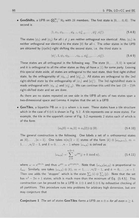
• GenTiles, a bipartite PB o n n ® n where n is even. These states have a tile structure
which in the case of 6 ® 6 is shown in Fig. 5.2. A tile represents one or more states. For
example, the tile in the upperleft corner of Fig. 5.2 represents 2 states each of which is
of the form
(a0|0) + c*i|l) + Q 2 |2)) <8> |0). (5.4.10)
The general construction is the following. One labels a set of n orthonormal states
as | 0 ) , . . . , \n— 1). One takes n(n/2 — 1) states of the form \k) ® \ujm^+i), m =
1 , . . . , n/2 — 1, and k = 0 , . . . , n — 1 where |wm^) is defined as
n / 2 - 1
\tOm,k) = ] T Jm\j + k mod n), (5.4.11) j=o
where u = éA7V'n and thus uj]m = etA^mln. Note that (wm,fc|wn,fc) i s proportional to
8mn. Similarly, one takes \wm,k) ®\k), m = 1 , . . . , n /2 — 1, and k = 0 , . . . , n — 1.
Then one adds the "stopper" which is the state ]T^ \i) ® V \j). Note that the set
has n2 — 2n + 1 states, which is much more than the minimum of Eq. (5.4.5). This
construction can be proved to be a UPB in 4 ® 4 and 6 ® 6 by exhaustive checking of
all partitions. This procedure runs into problems for arbitrary high dimension, but one
may conjecture that
Conjecture 1 The set of states GenTiles forms a UPB on n®n for all even n > 4.

5.4 Product Bases, Local Distinguishability and Bound Entanglement 99
B
0 ï 2 3 4 5 1 !
2 0 2 2
2 -
2
2 -
2
2 -
2
2
2 -
1
2
2
2
2 -
2
2 -
2
2 -
2 2
2 -
2 2
2
2
2 -
2
2
2 2
2
2
2
2
2 2 3
2
2
2
2 2
2
2
2 4
2
2
2
2 2
2
2
2 5 '
2
2 i
2
Figure 5.2: Tile structure of the bipartite 6 ® 6 UPB.
• Tensor powers of UPBs. The following theorem holds:
Theorem 3 Given two bipartite UPBs Si and 52 with members \ip}) = \a}) ® 1/3/},
i = l , Zi on m <g> m i anc/ members \ipf) = |a2) (gi |/?2), i = 1 , . . . , l2 on n2 •
respectively. The PB { | ^ ) ® | ^ | ) } ! l j = i 's a bipartite UPB on n i n 2 ® m im 2 . >m2
Proof Assume the contrary, i.e. there is a product state that is orthogonal to this new
ensemble which we call PB 2 . The idea is to show that this leads to a contradiction
and thus PB 2 is a UPB. Note first that for any UPB a partition P into a set with 0
states for Bob and all states for Alice give rise to a ppA (see Lemma 4) that has full
rank; the states on Alice's side together must span the entire Hilbert space of Alice.
Also note that if one takes a tensor product of two UPBs this partition in which all
states are assigned to Alice still leads to a ppA that has full rank on Alice's side as
Rank(p! <8> p2) = R.ank(pi)Rank(/92)-
The set PB 2 has lxl2 members. The new hypothetical product state to be added to the
set has to be orthogonal to each member either on Bob's side or on Alice's side, or on
both sides. One can represent such an orthogonality pattern as a rectangle of size lx
(number of columns) by l2 (number of rows) filled with the letters A and B, depending
on how the new state is orthogonal to a member of the PB 2 , see Fig. 5.3. When this
hypothetical state is orthogonal on both sides, we are free to choose an A or B in the
corresponding square. Consider a row of this rectangle. The pattern of As and the Bs can
be viewed as a partition of the Si UPB. For example in the partition of Sx corresponding
to the first row in Fig. 5.3 Alice gets the states \a\) and \a\) and Bob gets \ß\) and
\ß\),... , \ß\). Since S, is a UPB, either Alice's states span the full Hilbert space of
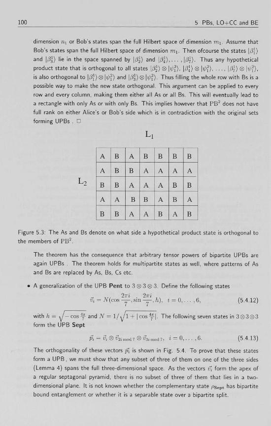
100 5 PBs, LO+CC and BE
dimension ni or Bob's states span the full Hubert space of dimension m i . Assume that
Bob's states span the full Hubert space of dimension m! . Then ofcourse the states \ß\)
and |/?3> lie in the space spanned by \ß\) and \ß\),... ,\ß\). Thus any hypothetical
product state that is orthogonal to all states \ß\) <g> \ip\), \ß\) ® \4>\) \ß}) ® \ip\),
is also orthogonal to \ß\)® \ipl) and \ß\)® \ipf). Thus filling the whole row with Bs is a
possible way to make the new state orthogonal. This argument can be applied to every
row and every column, making them either all As or all Bs. This will eventually lead to
a rectangle with only As or with only Bs. This implies however that PB 2 does not have
full rank on either Alice's or Bob's side which is in contradiction with the original sets
forming UPBs . D
L,
U
A B A B B B B
A B B A A A A
B B A A A B B
A A B B A B A
B B A A B A B
Figure 5.3: The As and Bs denote on what side a hypothetical product state is orthogonal to
the members of PB 2 .
The theorem has the consequence that arbitrary tensor powers of bipartite UPBs are
again UPBs . The theorem holds for multipartite states as well, where patterns of As
and Bs are replaced by As, Bs, Cs etc.
• A generalization of the UPB Pent to 3 ® 3 ® 3. Define the following states
2-ïïi 2iri Vi = N(cos—,sm~,h), i = 0,...,6, (5.4.12)
with h = J - cos y and N = 1 / v / l + | cos ^ | . The following seven states in 3<g)3(g>3
form the UPB Sept
Pi~Vi® «2imod7 <8> VZimodl, 1 = 0 , . . . , 6 . (5.4.13)
The orthogonality of these vectors pi is shown in Fig. 5.4. To prove that these states
form a UPB, we must show that any subset of three of them on one of the three sides
(Lemma 4) spans the full three-dimensional space. As the vectors v, form the apex of
a regular septagonal pyramid, there is no subset of three of them that lies in a two-
dimensional plane. It is not known whether the complementary state psept has bipartite
bound entanglement or whether it is a separable state over a bipartite split.
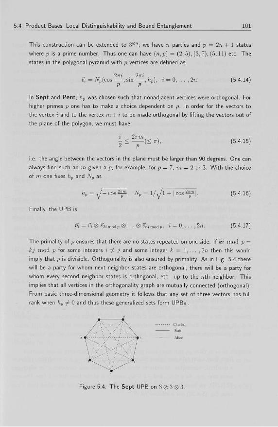
5.4 Product Bases, Local Distinguishability and Bound Entanglement 101
This construction can be extended to 3®"; we have n parties and p = In + 1 states
where p is a prime number. Thus one can have (n,p) = (2, 5), (3, 7), (5,11) etc. The
states in the polygonal pyramid with p vertices are defined as
2iri 2iri Vi = Np(cos ,sm ,hp), i = 0,...,2n. (5.4.14)
In Sept and Pent, hp was chosen such that nonadjacent vertices were orthogonal. For
higher primes p one has to make a choice dependent on p. In order for the vectors to
the vertex i and to the vertex m + i to be made orthogonal by lifting the vectors out of
the plane of the polygon, we must have
7T 2irrn, , ^ < — ( < T T ) , (5.4.15) z p
i.e. the angle between the vectors in the plane must be larger than 90 degrees. One can
always find such an m given a p, for example, for p = 7, m = 2 or 3. With the choice
of m one fixes hp and Np as
hp=yJ-cos2f±, Np = l/^l + \cos2-^\. (5.4.16)
Finally, the UPB is
Pi = vt® v2imod.p® •••®iimodp i i = Q, •••• ,2n. (5.4.17)
The primality of p ensures that there are no states repeated on one side: if ki mod p =
kj mod p for some integers i ^ j and some integer k = 1 , . . . , 2n then this would
imply that p is divisible. Orthogonality is also ensured by primality. As in Fig. 5.4 there
will be a party for whom next neighbor states are orthogonal, there will be a party for
whom every second neighbor states is orthogonal, etc. up to the nth neighbor. This
implies that all vertices in the orthogonality graph are mutually connected (orthogonal).
From basic three-dimensional geometry it follows that any set of three vectors has full
rank when hp / 0 and thus these generalized sets form UPBs .
Charlie
Bob
Alice
Figure 5.4: The Sept UPB on 3 <g> 3 <g> 3.
102 5 PBs, LO+CC and BE
• We would like to mention a conjecture by Peter Shor on the existence of a UPB based
on quadratic residues. These are sets of orthogonal product states on n ® n where n
is such that 2n — 1 is a prime p of the form Am + 1. Thus we can have (m,p, n) =
(1 , 5, 3), (3,13, 7) etc. The sets contains p = In — 1 members, the minimal number for
a UPB (Eq. (5.4.5)). Let Z* be Zp \ { 0 } . Let Qp be a group of quadratic residues,
that is, elements g G Z * such that
q = x2 mod p, (5.4.18)
for an integer x. The set Qp is a group under multiplication. The order of the group is
^ i . The following properties hold: when ci e Qp and q2 $. Qp, a quadratic nonresidue,
then qiq2 ^ Qp. Also, if qx <£ Qp and q2 <£ Qp, then qxq2 € Qp [127]. The states of the
UPB are
\Q{a)) <g> \Q(xa)) for a e Zp, xeZ;,x<£ Qp, (5.4.19)
where
|Q(a)) = (TV, 0, . . . , 0) + 5 3 e 2 ^ o / % , (5.4.20)
where AT is a normalization constant to be fixed for orthogonality and eq are unit vectors
of the form ( 0 , 1 , 0 , . . . ,0) , (0, 0 , 1 , 0 , . . . , 0) etc. The dimension n of the Hubert space
is ^ i i , one more than the order of Qp. One can prove that these vectors can be made
orthogonal by an appropriate choice of N:
(Q(a)\Q(b))(Q(xa)\Q(xb)) =
(\N\2 + Y2 e2,ri«(f,-a)/p)(|Ar|2 + 5 3 e27Tiqx(b-a)/p). (5.4.21)
q£Qp qeQp
One uses the properties of Qp to find that for (b — a) =/= 0:
V ^ e2iriq(b-a)/p _|_ V ^ e2iriqx(b-a)lp _ V ^ e2wiz(b-a)/p _ _ j /-g ^ 2 2 )
<?6QP q£Qp zez;
Thus the orthogonality relation of Eq. (5.4.21) for b ƒ a is of the form
( | A f + S ) ( | i V | 2 - l - S ) = 0, (5.4.23)
where
s = 5 3 e27rl'(i,-a)/p. (5.4.24) 9 £ Q P
Note that s can take two values depending on whether b — a is a quadratic residue or
a quadratic nonresidue. In order to show that s is real, one considers s* in which one
sums over —q. As q € Qp and - 1 G Qp when p is of the form 4m + 1 (see Theorem
82,[127]), we have that — q e Qp. Therefore s = s". Thus for all values that s can
take, Eq. (5.4.23) has a solution for AT.

5.4 Product Bases, Local Distinguishability and Bound Entanglement 103
Conjecture 2 (Shor) The states given in Eq. (5.4.19) and Eq. (5.4.20) on n®n with
2n — 1 a prime of the form Am + 1 with the appropriate value of N determined by the
solution ofEq. (5.4.23) form a UPB.
The proof will require the application of Lemma 4, that is, one must show that any set
of n states on either side spans the full n-dimensional Hubert space. This conjecture has
been proved fo rp = 5, p = 13 and p = 17. These sets form a generalization of the Pent
UPB that was presented in section 5.4.2 and Figure 5.1. Drawn as graphs as in Fig.
5.1, they are regular polygons, with a prime number p (of the form Am + 1) of vertices.
The elements of the quadratic residue group Qp correspond to the periodicity of the
vectors that are orthogonal on one side. For example, when p = 13, one has quadratic
residues 1, 3, 4, 9,10 and 12. Thus on, say, Alice's side, every vertex is connected to its
first neighbor (1), every vertex is connected with the 3rd neighbor (3) etc. On Bob's
side the orthogonality pattern follows from the quadratic nonresidues.
5.4.4 Global versus Local Rank
The construction of bound entangled states based on UPBs suggests that bound entangled
density matrices only come with a large rank. The idea is that when a basis is nearly complete,
it is always possible to extend the basis and therefore our construction fails. The following
theorem captures this observation and is relevant for any kind of bipartite bound entangled
state with PPT. The theorem was conjectured by the author and proved together with P.
Horodecki [128].
Theorem 4 Let p be a bipartite density matrix on HA ® W-B- Define RA = Rank(Try ip) and
similarly RB. Let R be the rank of p itself. If
max(RA, RB) > R, (5.4.25)
then p is distillable.
Proof First of all, one can observe that when III&X(RA, RB) > R the state has to be
entangled. Any separable state can be written as a convex combination of a set of product
states {\ipi, 4>i)}. The number of linearly independent states \ipi) which determines RA is a
lower bound on the number of linearly independent states \tl>i,(j)i) which determines R, and
similarly for RB.
Without loss of generality let RA be the largest local rank. Let PA = T r ^p in its diagonal
form be d i a g ( A i , . . . , A R ^ , 0 , . . . ,0) . One can apply a local filter [131] on Alice's side to the
state p
(W®l)p(Wl®l) PW - Tr(W®l)p(Wi<Z>iy ( 5 A 2 6 )
104 5 PBs, LO+CC and BE
where W = à\a,g{\/\f\[,... , l/y/\RA, 0 , . . . , 0) in the same basis as pA. The filtering corre
sponds to the performance of a POVM measurement by Alice. The operation elements of her
POVM measurements are cW and y/l — \c\2W^W where c is chosen such that 1 — |c |2W^W
has eigenvalues in the interval [0,1]. Then with probability pw = Tr (cW ® 1) p (c*W^ ® 1)
the state pw is obtained and with probability 1 - pw the filtering fails. Note that it is not
a problem to have a certain probability of failure in a distillation protocol as one will have
an arbitrary number of copies of the state. The reduced density matrix pAyv of the filtered
state pw has the same rank and its eigenvalues are equal to -^- or 0. The rank of p can only
decrease or stay the same by filtering. From this it follows that for any eigenvalue \PA w
W = iA < ^ < AST. (5-4.27)
where A ^ 1 is the largest eigenvalue of pw. Now we invoke a theorem in Ref. [131] which
says that any bipartite density matrix p for which there exists a pure state \xp) such that
{tP\{pA®l)-p\i>)<Q, (5.4.28)
is distillable. Take \tp) to be the eigenvector of pw with maximum eigenvalue and it follows
from Eq. (5.4.27) and Eq. (5.4.28) that pw and therefore p is distillable. This completes the
proof, ü
The consequence of this theorem is that there exists no bipartite bound entangled state
on any HA <8> HB that has rank 2. The reason is that when the maximum local rank of a
bipartite rank 2 density matrix p exceeds 2, Theorem 4 implies that the state is distillable. On
the other hand if both local ranks of p are smaller than or equal to 2, then the density matrix
p effectively has support only on a 2 ® 2 subspace. But it is known that all entangled density
matrices on 2 ® 2 are distillable [111].
It also follows that any bipartite PB S on n ® m with a number of states k = nm — 2
is extendible. By construction the complementary state ps has the PPT-property. However,
ps has rank 2 and there do not exist bound entangled states with rank 2. Therefore ps
must be separable and it follows that S is extendible. One can carry the argument one step
further. After adding the new product state to the set S, we can ask whether one can find
the last product state of the basis. Again, that state, which is a pure state must have the
PPT-property. It is not hard to show that all entangled pure state have the NPT-property
and therefore this last basis state must be a product state. Hence we have shown that any
bipartite PB S in H which has d im 'H — 2 states is not only extendible but also completable.
5.4.5 Local Distinguishability and Uncompletable Product Bases
lri the preceding sections we showed how UPBs give rise to entangled states that cannot be
distilled. It turns out that this is not the only interesting property that these sets of states have.
One can ask whether the members of a UPB are distinguishable by Local quantum Operations
and Classical Communication (LO+CC). The situation is the same as we described in section

5.4 Product Bases, Local Distinguishability and Bound Entanglement 105
5.4.1. We will consider sets of product states which are mutually orthogonal, such as the UPBs.
This implies that these states are distinguishable when arbitrary quantum measurements are
allowed. When the set of states is given by { |V" j ) ]>! i then a projection measurement with
projectors {TTJ = l ^ ' X ^ I } ^ and TTS± = 1 - Ylj^j w o u l d distinguish the states in the
set S. The question is whether measurements that exactly distinguish the set of states can
be implemented with local operations and classical communication only. Let us assume that
two parties Alice and Bob are given one of the five states in the Pent set and they have to
determine by LO+CC which one they have. It is not hard to see that for a set such as Pent
straightforward attempts at finding an appropriate series of measurements are bound to fail;
the way in which the states are made orthogonal, partially on Alice's side, partially on Bob's
side seems to preclude the existence of a perfect measurement. The parties seem to end up
with disturbing the states by measuring them and this disturbance then results in a set of
non-orthogonal product states that can no longer be distinguished.
On first state
^ s p a n ^ ^ )
Tlspan(B3,B4)
B
Done
Go to 2nd state 3 states left
Go to 2nd state 2 states left
Go to 2nd state 2 states left
Figure 5.5: Measurement tree for two copies of the Pent ensemble.
In order to understand what kinds of measurement protocols are possible, we consider the
situation in which the two parties are given two copies of the same state of the Pent set. We
can then show that there is a LO+CC that reliably identifies the states. This measurement
procedure is presented in Fig. 5.5. Each level of the tree corresponds to a measurement by
either Alice or Bob. After each measurement round Alice and Bob communicate classically
to discuss the results. In this protocol only (incomplete) von Neumann measurements (see
Chap. 3, sec. 3.2) are performed and they are denoted by their operation elements which are
projectors. The states of the P e n t set themselves are denoted as , 4 0 , . . . , A4 for Alice's part
of the Pent states and BO,... , B4 for Bob's part in correspondence with i — 0 , . . . , 4 in Eq.
(5.4.3). Thus in the first round Alice's measurement has two outcomes, associated with the
projector on her |0) state and the projector on the span of her |2) and |3) states, which obey
the relation
^O + 7TSpan(/13,yl2) = 1- ( 5 . 4 . 2 9 )
As one can see in Fig. 5.5 by a two-round protocol on the first state, Alice and Bob have
reduced the number of states to be distinguished to at most three. Now it is not hard to see that
106 5 PBs, LO+CC and BE
three orthogonal product states can always be distinguished by von Neumann measurements
(see also sec. 5.4.8).
One can associate with the leafs of such a measurement tree the series of projections that
resulted in the series of measurement outcomes. For example, in the tree of Fig. 5.5, the leaf
all the way to the left can be associated with the projector:
nAO®iTBo- (5.4.30)
These projectors at the ends of the tree are called 'leaf-projectors'. Aside from local von Neu
mann measurements a party can also perform local POVM measurements. But by Neumark's
theorem [62] any POVM measurement on a Hilbert space H can be viewed as an (incomplete)
von Neumann measurement in an extended higher dimensional Hilbert space Hext. When the
number of POVM outcomes is finite, this extended Hilbert space is finite. Note that the con
version of a local POVM to a local von Neumann measurement corresponds to a local extension
of the Hilbert space, i.e. for a bipartite system a Hilbert space H = HA®HB'^ extended to
Uext = {HA © H'A) 0 (KB © H'B) where U\ and H'B are the extensions of the local Hilbert
spaces HA and HB- In the following analysis the local measurements are restricted to have a
finite number of outcomes. Furthermore we require that the number of rounds in the entire
protocol is finite. Thus one can say that we restrict ourselves to finite resources in time and
space. Every local measurement with a finite number of outcomes can be decomposed into a
series of local measurements with two outcomes only with the understanding that subsequent
levels of the measurement tree can correspond to actions of the same party.
A special class of local measurements are the measurements that we call dissections. A
dissection measurement is one in which the set of states S is split into two sets 1 and 2. The
states themselves are unchanged by the measurement, but the outcome of the measurement
tells us whether the state that one is given was in set 1 or in set 2. More general measurement
schemes can project the states in S onto other states that might or might not be orthogonal.
In the last section we briefly mentioned the notion of a completion of a set of orthogonal
product states. Let us now give the definition of an uncompletable set of orthogonal product
states.
Definition 6 Consider a multipartite quantum system H = ( 8 ) ™ ! % with m parties of re
spective dimension di,i = 1, ...,m. An uncompletable product basis in H is a PB that cannot
be completed with orthogonal product states to a full orthonormal product basis for H.
Remark The uncompletable product basis is defined with respect to H. An orthogonal
product basis in H could be uncompletable in H, but computable to a full product basis for
Hext, when the set is embedded in Hext. In section 5.4.6 we will give an example of such a
set.
The following theorem captures an essential connection between completability and exact
local distinguishability:
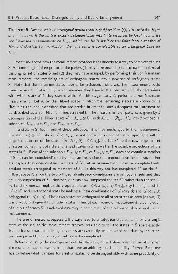
5.4 Product Bases, Local Distinguishability and Bound Entanglement 107
Theorem 5 Given a set 5 of orthogonal product states (PB j on% = ® •" l Hi with d im'H, =
di,i = l,...,m. If the set S is exactly distinguishable with finite resources by local incomplete
von Neumann measurements on 7iext,-which can be H itself or any finite local extension of
H-, and classical communication, then the set S is computable to an orthogonal basis for
next-
Proof One shows how the measurement protocol leads directly to a way to complete the set
S. At some stage of their protocol, the parties (1) may have been able to eliminate members of
the original set of states S and (2) they may have mapped, by performing their von Neumann
measurements, the remaining set of orthogonal states into a new set of orthogonal states
S'. Note that the remaining states have to be orthogonal, otherwise the measurement could
never be exact. Determining which member they have in this new set uniquely determines
with which state of S they started with. At this stage, party i0 performs a von Neumann
measurement. Let K, be the Hubert space in which the remaining states are known to lie
(including the local extensions that are needed in order for any subsequent measurement to
be described as a von Neumann measurement). The measurement of party io is given by a
decomposition of the Hilbert space K. = K,eise®K-ia with ICeise = <3),-=ü /CJ, into 2 orthogonal
subspaces, K-else ® 7Ti/Cio and Kelse <g> n2JC1Sj.
If a state in S' lies in one of these subspaces, it will be unchanged by the measurement.
If a state \a) ® \ß), where \a) G fCeise, is not contained in one of the subspaces, it will be
projected onto one of the states {\a) <g>7Ti|/?), \a) ® 7r2|/3)}. Let S" be this new projected set
of states, containing both the unchanged states in S' as well as the possible projections of the
states in S'. If one of the subspaces lCeise<8>niJCi0 or /Ce/se<8> 7r2/Ci0 does not contain a member
of S', it can be 'completed' directly; one can freely choose a product basis for this space. For
a subspace that does contain members of S", let us assume that it can be completed with
product states orthogonal to members of S". In this way one has completed S" on the full
Hilbert space fC since the two orthogonal-subspace completions are orthogonal sets and they
are a decomposition of K-. However, one has now completed the set S" rather than the set S'.
Fortunately, one can replace the projected states \a) ®TTi\ß), \a) ® 7r2|/3) by the original state
|a )® 1/3) and 1 orthogonal state by making a linear combination of |a)<g>7Ti|/3) and |a)®7r2|/3)
orthogonal to |a)®|/?) . These two states are orthogonal to all other states as each \a)®iri\ß)
was already orthogonal to all other states. Thus at each round of measurement, a completion
of the set of states S' is achieved assuming a completion of the subspaces determined by the
measurement.
The tree of nested subspaces will always lead to a subspace that contains only a single
state of the set, as the measurement protocol was able to tell the states in S apart exactly.
But such a subspace containing only one state can easily be completed and thus, by induction,
we have proved that the original set S can be completed. D
Before discussing the consequences of this theorem, we will show how one can strengthen
the result to include measurements that have an arbitrary small probability of error. First, one
has to define what it means for a set of states to be distinguishable with some probability of
108 5 PBs, LO+CC and BE
error:
Definition 7 Given a set S of orthogonal product states (PB) on H = (g)™^ Hi with
dimHi = d,,i = l,...,m. Let A4 be a local incomplete von Neumann measurement pro
tocol on a finite-dimensional Hilbert space Hext which can be a local extension of H, that
includes classical communication between the local parties. Let V(M) be a decision scheme
that associates each leaf of the measurement tree of M with a state of the set S, meaning
that upon the outcomes of leaf j, we decide that the associated state i is the state that we
were given of the set 5. A set 5 is e-distinguishable if there exists an M and a V(M) such
that
PsucM = min J2 Prob(7Tj|i) > 1 - e, (5.4.31) j I i-*i
where it\,... ,irk are the leaf-projectors of the measurement tree of M. Prob(7rJ|i) is the
probability that given the state i we obtain the measurement outcomes of leaf ITr The sum
over the leaf-projectors is constrained to leaf-projectors that lead to deciding for state i, which
is indicated by j —> i.
In words this definition says that the set S is e-distinguishable if the probability of deciding
correctly for a state in S is greater than or equal to 1 - e for any state that the parties are
given from S. This definition makes it possible to state the following lemma:
Lemma 5 Given a set S of orthogonal product states (PR) on H = (g)™ l Hi with dimH, =
di,i = 1, . . . ,m . If the set S is e-distinguishable for all e > 0 then S is exactly distinguishable.
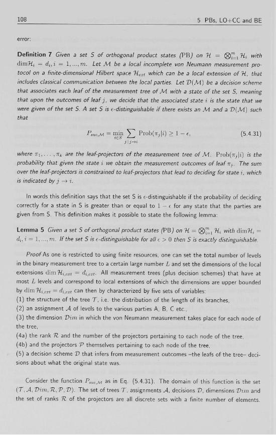
Proof As one is restricted to using finite resources, one can set the total number of levels
in the binary measurement tree to a certain large number L and set the dimensions of the local
extensions d im% ) < K r t = di<ext. All measurement trees (plus decision schemes) that have at
most L levels and correspond to local extensions of which the dimensions are upper bounded
by dim'Hi.eit = dit<,xt can then by characterized by five sets of variables:
(1) the structure of the tree T , i.e. the distribution of the length of its branches,
(2) an assignment A of levels to the various parties A, B, C etc.,
(3) the dimension Vim in which the von Neumann measurement takes place for each node of
the tree,
(4a) the rank K and the number of the projectors pertaining to each node of the tree,
(4b) and the projectors V themselves pertaining to each node of the tree,
(5) a decision scheme V that infers from measurement outcomes - the leafs of the tree- deci
sions about what the original state was.
Consider the function PsucM as in Eq. (5.4.31). The domain of this function is the set
( T , A, Vim, H, V, V). The set of trees T , assignments A, decisions V, dimensions Vim, and
the set of ranks 1Z of the projectors are all discrete sets with a finite number of elements.

5.4 Product Bases, Local Distinguishability and Bound Entanglement 109
Consider a measurement at a single node. We fix the number of projectors, the dimension of
the Hubert space and the rank of the projectors at this node. Let (7^,7^) be a set of projectors
at this node. Then another set (7^, n'2) can be obtained by unitary transformations U^i = 7T-.
This implies that the set (7T1,7T2) is a compact set, as the set of unitary transformations in a
finite-dimensional Hubert space is a compact set. The function PSUC,M is continuous on this
compact set. The entire domain of the function PSUC:M is the union of a finite number of
compact sets. Then, if there exists measurements and decision schemes such that PSUC,M is
larger or equal than 1 — e for all e, there also exist a scheme for which PSUC,M = 1- This
measurement corresponds to exactly distinguishing the members of S. O
Corollary 1 Given a set S of orthogonal product states (PB) on% = ®™-! "Hi with d i r n % =
di, 7 = 1 , . . . , m. If this set S is e-distinguishable for all e > 0, then 5 is exactly computable on
7iext, a locally extended Hilbert space or % itself.
This follows from Theorem 5 and Lemma 5.
Let us give a final theorem, that relates the question of completability to the property of
entanglement:
Theorem 6 Given a set S of orthogonal product states (PB j on H = (Q^ % Wlth diuiHi =
di, i = l, •••, m. If the set 5 is e-distinguishable for all e > 0, then the complementary density
matrix ps, Eq. (5.4.6), is separable.
Proof If the exact measurement is a von Neumann measurement on H, then by Corollary
1 the set S can be completed with product states to a basis for H. Thus, the density matrix
ps which is the uniform mixture of these product states that complete S, is separable. If the
exact measurement is a von Neumann measurement on l~iRXt, then the density matrix ps,ext
is separable. One can obtain ps on H by local projections from fiext onto T-L and therefore
ps = PnPs,extPn is separable as well. D
This theorem implies that a multipartite UPB S is not distinguishable with arbitrary small
probability of error by LO+CC, using finite resources, since the density matrix ps is entangled.
The UPBs are new illustrations of the phenomenon of nonlocality without entanglement. The
strength of the result as compared to the results in Ref. [125], is that the indistinguishability
has been proved for any UPB, whereas in Ref. [125] only the set of states of Eq. (5.4.1)
were shown not to be distinguishable with arbitrary small probability of error. The weakness
of this result is that we have restricted the set of measurements to ones that can be performed
using finite resources. This was necessary as a POVM measurement with an infinite number
of outcomes describes a von Neumann measurement in an infinite dimensional Hilbert space.
It is not clear how to extend the notions of completability on an infinite dimensional Hilbert
space. Also, it is unclear whether a result such as Lemma 5 would hold for measurements that
could use infinite resources.

H Ç 5 PBs, LO+CC and BE
5.4.6 Local Extensions and Deficits of Product States
In the last section care has been taken to include POVM measurements in a local measurement
scheme. But do there exist PBs that are exactly distinguishable by POVMs but not by von
Neumann measurements in the original Hubert space? It turns out that there are such sets.
Here is an example of such a set on 3®4, the set PO. Consider the states Vj<g>Wj, j = 0 , . . . ,4
with Vj the states of the Pent UPB as in Eq. (5.4.2) and Wj defined as
Wj = y2/^/5(y/cœ^iJ^cos(2jn/5),^l/cös^KJ5)sm(2j^^/5),
y/cos(2ir/5) cos(4jn/5), ^/cos(27r/5)sin(4J7r/5)). (5.4.32)
Note that wjwj+i = 0 (addition mod 5). The orthogonality graph of these states is the
same as for Pent, Figure 5.1. One can show that this set, albeit extendible on 3 ® 4, is not
computable: One can at most add three vectors: v0 ® (w0, wr, W4)1, v3 ® (w2, w3, w^)1 and
{vcVz)1 ® ( w ^ u J j , ^ ) 1 -
The POVM measurement that is performed by Bob on the four-dimensional side has five
projector elements, each projecting onto a vector
u3 = -^(-sin(2j7r /5) ,cos(2J7r/5) ,-s in(4J7r/5) ,cos(4J7r/5)) ! (5.4.33)
with j = 0 , . . . ,4 . Note that u0 is orthogonal to vectors w0,w2 and w3, or, in general,
«j is orthogonal to Wi,wi+2,wi+3 (addition mod 5). This means that upon Bob's POVM
measurement outcome, three vectors are excluded from the set; then the remaining two vectors
on Alice's side, vi+l and vi+4, are orthogonal and can thus be distinguished.
Since the set is distinguishable by a POVM, it is computable. The completion of this
set in 3 ® 5 is particularly simple. Bob's Hubert space is extended to a five-dimensional
space. The POVM measurement can be extended to a projection measurement in this five-
dimensional space with orthogonal projections onto the states £ = ( K , , 0 ) + | ( 0 , 0 ,0 ,0 ,1) .
Then a completion of the set in 3 ® 5 are the following ten states:
{vo-,^)-1 ® Xx
{vuv3)^ ®x2
(v2, n)-1 ® £3
(uo,tf3)-L®£4
v0 ® {WQ e Span(£4, Xi)),
vi ® (w^ e Span(£0 ,£2)),
v2 ® {w% E Span (f i , £3)), (5.4.34)
v3 ® (w^ G Span(£2 ,£4)) ,
VA ® (wj- e Span(£3, £0)).
There is another interesting feature of this set. Let's take the set PO and add one of the
product states, say the vector,
u 0 ® (wojWuWt)1, (5.4.35)
to make it a six-state ensemble PO+. The complementary density matrix p P O +, Eq. (5.4.6),
has rank 1 2 - 6 = 6. Is pP O+ a separable density matrix? We can enumerate the product states

5.4 Product Bases, Local Distinguishability and Bound Entanglement 111
that are orthogonal to the members of P O + , but are not necessarily mutually orthogonal:
«2® (wu^ws)-1, (5 4 36) {vo,v3)
±^(wi,W2,wi)-L,
{vo,^)1 ® (ùJi ,^,^)-1- .
This means that the space on which pPo+ has support contains only four product states,
whereas pPO+ has rank 6. Therefore pP O+ m u s t be entangled. The entanglement of pPO+ is
bound by construction.
We have constructed a new bound entangled state whose range is not without product
states but has a product state deficit. As any UPB set, the set P O + is not locally distinguish
able with finite means. This construction works in a very general way:
Lemma 6 Given a set S of orthogonal product states f P B j on 7i = ® ™ , Hi with dimHi =
di,i = 1, ...,m. If the set S is not computable to a full basis for H, but is completable in
some Hext, then there always exist a set of orthogonal product states in Jig such that when
we add these states to S to make the ensemble S+, the complementary density matrix ps+ is
bound entangled.
Proof Assume that there does not exist such an augmented ensemble S + . This will lead
to a contradiction. The fact that S is completable in Hext makes it possible to add at least
one product state to S, see Theorem 6. Let us call this state |V>i). The density matrix p ^
complementary to the ensemble S\ = S U { l ^ i ) } 's either entangled or separable. If it is
entangled, then we have found the desired augmentation of S. If it is separable, then there
is at least one state, let us call it |J/)2), in the range of ps t which is a product state. Note
that jv2) is orthogonal to \ipi)- Then we can augment pst with this new orthogonal product
state \tp2) to make the set ps2. Consider its complementary density matrix pS2. Repeat the
arguments as before. If we find that all density matrices psl,Ps2> • • • >PSdimw-isi a r e separable,
then we have found a completion of the original set S with orthogonal product states. This
leads to a contradiction, because S is not completable in %. •
Remark While the lemma shows that there exists a set of orthogonal product states that
when added to the set S leads to a bound entangled state, the proof also suggests a simple
way to find this set. The bound entangled state that we find by this procedure can be a bound
entangled state corresponding to a UPB, that is the augmented set S + is a UPB, or it can be
an entangled state, based on a set such as P O + , which is supported on a subspace which has
a product state deficit.
5.4.7 Rank and the Opt imal Decomposit ion of a Density Matr ix
Some of the uncompletable sets of product states exhibit additional interesting properties.
It was shown by Uhlmann [132] that every bipartite density matrix p admits an optimal de
composition, that is, a decomposition that achieves the entanglement of formation E(p), Eq.

112 5 PBs, LO+CC and BE
(5.2.11), with at least Rank(p) and at most Rank(p)2 different pure states. No examples
of density matrices for which more than Rank(p) states are needed to construct the optimal
decomposition were previously known. By numerical minimization it was found that the state
complementary to the Tiles UPB , as introduced in section 5.4.2, has an entanglement of
formation of 0.213726 bits. This complementary state pTiies has rank 4. However, it was
found that the optimal ensemble of pure states consists of five pure states. A similar result
was found for the Pent UPB which has an entanglement of 0.232635 bits, made by mixing
together five pure states. Thus both these density matrices are numerical examples of states
for which more states are needed in the optimal decomposition than the rank of the state.
The following result exhibits a whole class of separable states which have this peculiar
property.
Theorem 7 Let {\ar) ® | $ ) } f c i t e a PB S in -H = HA® HB- If S is uncompletable in H,
but 5 is completable in some local extension %ext ofH, then ps has the property that the
number of different pure states in the optimal decomposition of ps exceeds the rank of ps.
Proof Since the set of states S is completable in a local extension of H, the state ps
is separable by Theorem 6. However we know that ps was uncompletable in H, therefore
Ps cannot be decomposed with an ensemble of orthogonal product states. Any optimal
decomposition of ps has to use nonorthogonal product states. The von Neumann entropy
of ps is equal to S(ps) = logRank(p s ) as ps is the identity matrix on a space of dimension
Rank(,o5). In order to achieve this entropy the optimal decomposition of ps has to use
more than Rank(p s ) product states, as any density matrix p which is a mixture of only n
non-orthogonal states has entropy strictly less than l ogn bits. D
The only example so far is the set PO in 3 <g> 4, which was distinguishable by a set of
orthogonal projectors in 3 ® 5, but could not be completed in 3 <g> 4. The complementary
density matrix pPO on 3 <g> 4 has rank seven, but the separable decomposition consists of ten
non-orthogonal states. These ten non-orthogonal product states are obtained by projecting
the orthogonal states of the completion, Eq. (5.4.34) back into the 3 ® 4 Hubert space. It is
not known whether there exists a separable decomposition with more than seven but with less
than ten states.
5.4.8 Restrictions
The method to create bound entangled states from UPBs is not always successful. In particular
one can show that
Theorem 8 Any set of orthogonal product states { |a;) ® \ßi)}%=1 in 2 <g> n for any n > 2 is
distinguishable by local measurements and classical communication and therefore completable
to a full product basis for2®n.
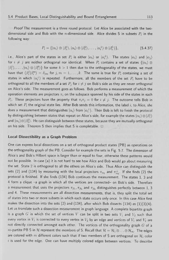
5.4 Product Bases, Local Distinguishability and Bound Entanglement 113
Proof The measurement is a three round protocol. Let Alice be associated with the two-
dimensional side and Bob with the n-dimensional side. Alice divides S in subsets Pt in the
following way:
Pt = ( K ) ® | # ) , \ai) ® \ßf),..., \cxj-) ® I/?}')}, (5.4.37)
i.e., Alice's part of the states in set Pt is either |OJ) or la/-). The states |QJ) and la,)
for i ^ j are neither orthogonal nor identical. When Pt contains a set of states { |a j ) <g>
| /? / ) , . . . , |ûi) <S> \ßi)} for some /c > 1 then due to the orthogonality of the states, we must
have that (/?ƒ |/3™) = 5]m for j,m = 1 , . . . ,k. The same is true for Pz containing a set of
states in which \aj~) is repeated. Furthermore, all the members of the set P, have to be
orthogonal to all the members of a set Pj for i ƒ j on Bob's side as they are never orthogonal
on Alice's side. The measurement goes as follows. Bob performs a measurement of which the
operation elements are projectors TTJ on the subspace spanned by his side of the states in each
Pi. These projectors have the property that n^j = 0 for i ^ j. The outcome tells Bob in
which set Pi the original state lies. After Bob sends this information, the label i, to Alice, she
does a measurement that distinguishes |aj) from \al). Then Bob is left to finish the protocol
by distinguishing between states that repeat on Alice's side, for example the states |ai)<g> \ß{)
and \ai)tg>\ßf). He can distinguish between these states, because they are mutually orthogonal
on his side. Theorem 5 then implies that S is computable. D
Local Dissectibility as a Graph Problem
One can express local dissections on a set of orthogonal product states (PB) as operations on
the orthogonality graph of the PB. Consider for example the sets in Fig. 5.7. The dimension of
Alice's and Bob's Hubert space is larger than or equal to four, otherwise these patterns would
not be possible. In case (a) it is not hard to see how Alice and Bob would go about measuring
the set. State 2 is orthogonal to all the others on Alice's side. Thus Alice can distinguish the
sets (2) and (134) by measuring with the local projectors na2 and TT^. If she finds (2) the
protocol is finished. If she finds (134) Bob continues the measurement. The states 1, 3 and
4 form a clique -a graph in which all the vertices are connected- on Bob's side. Therefore
a measurement that uses the projectors Tr01,n03 and ir0i distinguishes perfectly between 1, 3
and 4. These measurements are all dissection measurements, that is, they split the total set
of states into two or more subsets in which each state occurs only once. In this case Alice first
makes the dissection into the sets (2) and (134), after which Bob dissects (134) as (1)(3)(4).
Let us translate such a dissection measurement in graph language. A complete bipartite graph
is a graph G in which the set of vertices V can be split in two sets Vj and V2 such that
every vertex in \\ is connected to every vertex in V2 by an edge and vertices of \\ and V2 are
not directly connected amongst each other. The vertices of the orthogonality graph G of a
m-partite PB S in % represent the members of S. Recall that H = Ui®.. . ® H m . The edges
are colored with m different colors such that if two members of S are orthogonal on ?^ color
i is used for the edge. One can have multiply colored edges between vertices. To describe
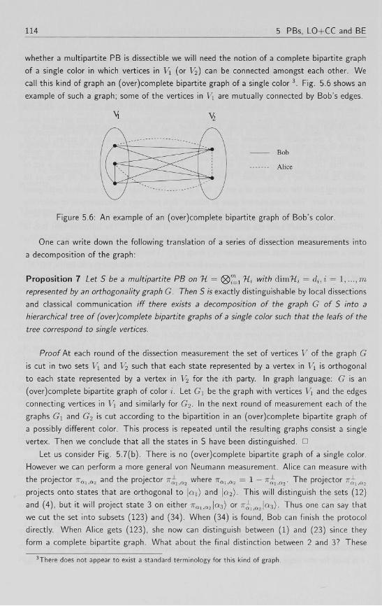
114 5 PBs, LO+CC and BE
whether a multipartite PB is dissectible we will need the notion of a complete bipartite graph
of a single color in which vertices in V\ (or V2) can be connected amongst each other. We
call this kind of graph an (over)complete bipartite graph of a single color3 . Fig. 5.6 shows an
example of such a graph; some of the vertices in Vj are mutually connected by Bob's edges.
Bob
Alice
Figure 5.6: An example of an (over)complete bipartite graph of Bob's color.
One can write down the following translation of a series of dissection measurements into
a decomposition of the graph:
Proposition 7 Let S be a multipartite PB on H = ® ™ L Hi with d im'H; = di, i = 1 , . . . , m,
represented by an orthogonality graph G. Then S is exactly distinguishable by local dissections
and classical communication iff there exists a decomposition of the graph G of S into a
hierarchical tree of (over)complete bipartite graphs of a single color such that the leafs of the
tree correspond to single vertices.
Proof At each round of the dissection measurement the set of vertices V of the graph G
is cut in two sets \\ and V2 such that each state represented by a vertex in \'\ is orthogonal
to each state represented by a vertex in V2 for the i th party. In graph language: G is an
(over)complete bipartite graph of color ?.. Let G\ be the graph with vertices Vj and the edges
connecting vertices in V\ and similarly for G2. In the next round of measurement each of the
graphs G\ and G2 is cut according to the bipartition in an (over)complete bipartite graph of
a possibly different color. This process is repeated until the resulting graphs consist a single
vertex. Then we conclude that all the states in S have been distinguished. O
Let us consider Fig. 5.7(b). There is no (over)complete bipartite graph of a single color.
However we can perform a more general von Neumann measurement. Alice can measure with
the projector -naim and the projector n^ Q2 where 7rQl]Q2 = 1 - 7r^ iQ2. The projector 7 ^ a2
projects onto states that are orthogonal to \a\) and \a2) • This will distinguish the sets (12)
and (4), but it will project state 3 on either 7TQ1:Q2 |Q'3) or 7 ^ Q2 |as). Thus one can say that
we cut the set into subsets (123) and (34). When (34) is found, Bob can finish the protocol
directly. When Alice gets (123), she now can distinguish between (1) and (23) since they
form a complete bipartite graph. What about the final distinction between 2 and 3? These
3There does not appear to exist a standard terminology for this kind of graph.
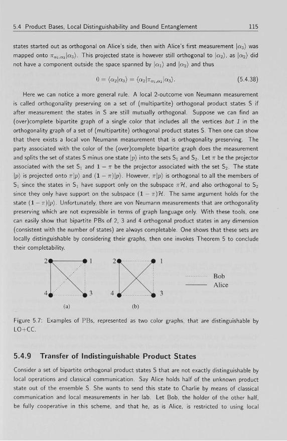
5.4 Product Bases, Local Distinguishability and Bound Entanglement 115
states started out as orthogonal on Alice's side, then with Alice's first measurement \a3) was
mapped onto 7rQ l i a 2 |a3) . This projected state is however still orthogonal to laç), as |a2) did
not have a component outside the space spanned by \ai) and |a2) and thus
0 = (a2\a3) = (U^KQLCJO-S) - (5.4.38)
Here we can notice a more general rule. A local 2-outcome von Neumann measurement
is called orthogonality preserving on a set of (multipartite) orthogonal product states S if
after measurement the states in S are still mutually orthogonal. Suppose we can find an
(over)complete bipartite graph of a single color that includes all the vertices but 1 in the
orthogonality graph of a set of (multipartite) orthogonal product states S. Then one can show
that there exists a local von Neumann measurement that is orthogonality preserving. The
party associated with the color of the (over)complete bipartite graph does the measurement
and splits the set of states S minus one state \p) into the sets Si and S2. Let IT be the projector
associated with the set Si and 1 — n be the projector associated with the set S2. The state
\p) is projected onto 7r|p) and (1 — 7r)|p). However, TT\P) is orthogonal to all the members of
Si since the states in Si have support only on the subspace TTT-L, and also orthogonal to S2
since they only have support on the subspace (1 — 71")%. The same argument holds for the
state (1 — 7T)|P). Unfortunately, there are von Neumann measurements that are orthogonality
preserving which are not expressible in terms of graph language only. With these tools, one
can easily show that bipartite PBs of 2, 3 and 4 orthogonal product states in any dimension
(consistent with the number of states) are always completable. One shows that these sets are
locally distinguishable by considering their graphs, then one invokes Theorem 5 to conclude
their completability.
1
Bob Alice
(a) (b)
Figure 5.7: Examples of PBs, represented as two color graphs, that are distinguishable by
LO+CC.
5.4.9 Transfer of Indistinguishable Product States
Consider a set of bipartite orthogonal product states S that are not exactly distinguishable by
local operations and classical communication. Say Alice holds half of the unknown product
state out of the ensemble S. She wants to send this state to Charlie by means of classical
communication and local measurements in her lab. Let Bob, the holder of the other half,
be fully cooperative in this scheme, and that he, as is Alice, is restricted to using local
116 5 PBs, LO+CC and BE
measurements and classical communication. We will show that when the states in S cannot
be locally distinguished, Alice will not be able to transfer her state exactly to Charlie. In
a scenario where Alice and Bob share some classically correlated information, it is always
possible for Alice to transmit this correlation to a third party, even when Alice and Bob are
ignorant about the information that they share. In the quantum scenario we ask whether
it is possible for Alice to transfer her half of an unknown product state which is correlated
with Bob to a third party, possibly in a way that does not reveal to Alice which state she
transferred. If Alice and Bob could measure what state they have, then it is clear that the
information about the state can be transferred from Alice to Charlie. They convert their
correlated quantum state to a piece of classical information. However, when Alice and Bob
cannot tell with absolute certainty what state they have, even though it is a product state,
it is not possible to transfer Alice's part to Charlie. The reason is the following. If it could
be achieved by means of classical communication and local measurements only, then all the
classical information that Alice sends to Charlie might as well be sent to Bob. Thus if Charlie
can reconstruct half of the state with this information, then so can Bob. Now Bob, possessing
both parts of the product state, does a local projection measurement on the orthogonal states
in S. Since the states are orthogonal this measurement will uniquely determine which state in
S he shared with Alice. This is in contradiction with the premise that the states in S are not
exactly distinguishable by LO+CC. What this construction illustrates is that even though no
entanglement is involved, the quantum states that the two parties share exhibit some essential
nonlocal quantum features.
5.4.10 The Use of Separable Superoperators
We have shown in the last sections that there exist sets of orthogonal product states that are
not locally distinguishable. In this section we address the question of what kind of measurement
does distinguish them. We are interested in finding measurements that need the least amount
of resources in terms of entanglement between the two or more parties.
Let us introduce a class of quantum operations that are close relatives of operations that
can be implemented by local quantum operations and classical communication, the separable
superoperators and measurements:
Definition 8 [133]LetH = <g>"= i%- LetW = <g>"=1 %[. A T C P mapS: B{H) ->• B{H')
is separable iff one can write the action of S on an arbitrary density matrix p e B(H) as
S{P) = Yl A^ ® Ä2'' ® • • • ® An'< P AU ® AU ® • • • ® AU' (5.4.39) i
where .4^ , is a d im?^ x dimHi matrix and
]T A\tAhl ® A\tlA2<l ® . . . ® Al^i = 1. (5.4.40)

5.4 Product Bases, Local Distinguishability and Bound Entanglement 117
Similarly, a quantum measurement (Chap. 3, sec. 3.2) on a multipartite Hilbert space is
separable iff for each outcome m, the operation elements A™ for alii are of a separable form:
AT = A™ ® A% ® . . . ® A™{. (5.4.41)
The results of [125] show that separable superoperators are not equivalent to local quantum
operations and classical communication. There is a separable measurement for the nine states
of Eq. (5.4.1); it is the measurement whose operation elements are the projectors onto the
nine states. The nine states are not locally distinguishable by LO+CC.
The following theorem gives a sufficient condition under which a bipartite set of orthogonal
product states is distinguishable with the use of separable measurements. Unfortunately, it
is not known what entanglement resources are needed to implement such separable measure
ments. They do however form a rather restricted class of operations. It is for example not
possible to use them to create entanglement where previously none existed.
Theorem 9 Let S be a set of bipartite orthogonal product states in H = HA ® HB with k
members. If S has the property that it is completable in % or local extensions of % (Hext)
when any single member is removed from S, then the members of S are distinguishable by
means of a separable measurement.
Proof Denote by {7Ti}f=1 the orthogonal rank 1 product projectors onto the states in S.
Let Si be the set S without a state i. As S is completable, the projectors
7Tsx = l - ^ 7 r m , (5.4.42)
for all i = 1 , . . . , k, are separable. Note that -KSL = 7TL . The projectors ns± and 7TJ for
i = 1 , . . . , k with the right coefficients sum up to 1:
l Ê * W + k-ïr È *& = *> (5 A 4 3) k i=l
using 7T2 = 7T for projectors. As the projectors TTS± are separable, one can decompose them
into a set of Ni rank 1 product projectors, 7T/S± •, labeled by an index mi = 1 , . . . , iVj.
Note that one can choose mutually orthogonal projectors (for a given i) TT,S± m.N when S, is
completable in the given Hilbert space H. When S; is completable only in a local extension
of 7i, these projectors will be non-orthogonal. In both cases the set of product projectors
are the operation elements of a separable measurement. This measurement projects onto
states in S or onto separable states that are orthogonal to all but one state in S. With a slight
118 5 PBs, LO+CC and BE
modification of this measurement one can construct a measurement which distinguishes the
states in S locally. Formally one replaces the projectors of Eq. (5.4.44) by
iï = \oti,ßi)(ai,ßi\ -> \iA,iB){<*ußi\, (5 4 451 %{S±,mi) = l(5i,m,,7i,m,)(<5j,m,,7I,mi| -> \l', 77llA, i', miB) (<5,,mi, ^mi |,
such that the set of states \iA), \i'imiA} 's a n orthonormal set and the same for B. This
modification leaves Eq. (5.4.43) unchanged, so that this new set of operation elements again
corresponds to a (separable) measurement. Upon this measurement, however, Alice and Bob
both get a classical record of the outcome. If they perform this measurement on states in S,
their outcomes will uniquely determine which state in S they were given. •
Both the Pent UPB as well as the Tiles UPB are examples of sets that are completable
in 3 ® 3 when anyone state in the set is omitted. These sets are thus distinguishable by a
separable measurement.
5.5 A Family of Indecomposable Positive Linear Maps
We introduce a new family of indecomposable positive linear maps based on entangled states.
Central to our construction is the notion of an unextendible product basis. The construction
lets us create and conjecture indecomposable positive linear maps in matrix algebras of arbitrary
high dimension.
5.5.1 Introduction
One of the central problems in the emergent field of quantum information theory [37] is the
classification and characterization of the entanglement of quantum states. Entangled quantum
states have been shown to be valuable resources in (quantum) communication and computation
protocols. In this context it has been shown [112] that there exists a strong connection between
the classification of the entanglement of quantum states and the structure of positive linear
maps. Very little is known about the structure of positive linear maps even on low dimensional
matrix algebras, in particular the structure of indecomposable positive linear maps. We denote
the n x n matrix algebra as M „ ( C ) . The first example of an indecomposable positive linear
map in M 3 ( C ) was found by Choi [134]. There have been only a couple of other examples of
indecomposable positive linear maps (see Ref. [135] for some recent literature); they seem to
be hard to find and no general construction method is available. In this section we make use
of the connection with quantum states to develop a method to create indecomposable positive
linear maps on matrix algebras M „ ( C ) for any n > 2. This construction exhibits some of the
structure of positive linear maps which is present in almost any dimension. In section 5.5.2 we
present the general construction. In section 5.5.3 we present two examples and discuss various
open problems.

5.5 A Family of Indecomposable Positive Linear Maps 119
5.5.2 Unextendible Product Bases and Indecomposable Maps
The more complicated structure of the positive linear maps in higher dimensional matrix
algebras, namely the existence of indecomposable positive maps (see the introductory section
5.2.3) is reflected in the existence of entangled density matrices p on HA ® HB for which
(id,4 ® T ) (p) is positive semidefinite.
In Ref. [136] a method was discovered to construct entangled density matrices p with
positive semidefinite ( i d^ (g> T) (p) in various dimensions d im HA > 2 and d im "HB > 2. The
construction was based on the notion of an unextendible product basis.
We will present our results relating these density matrices obtained from the construction
in Proposition 6 to indecomposable positive linear maps. We will need the definition of a
maximally entangled pure state:
Definition 9 LetH = HA® "HB- i-et \ip) be a normalized state ( ( V # ) = 1) ' " ^ and
PA,* = TrB\il>){il>\, (5.5.1)
where T r B indicates that the trace is taken with respect to Hubert space HB only. The state
\I/J) G H is maximally entangled if
S{PA,V) = -Tr pA,i> log2 pA,i, = log2min(dim?i/1,dimHB) (5.5.2)
The function S{pA^) is the von Neumann entropy of the density matrix pA,^-
Remarks For pure states \ip) the von Neumann entropy of pA,ip is always less than or
equal to d = log2 m in (d im 'Hy i ,d im 'H B ) . For maximally entangled states we will have
PA,i> = d i a g ( l / d , . . . , 1/d, 0 , . . . , 0) so that the maximum von Neumann entropy, Eq. (5.5.2),
is achieved. When d i m ? ^ = d im H B one can always make an orthonormal basis for ~H with
maximally entangled states [137]. For pure states |i/>) we always have S(PA^) = S(pB,^)-
The following lemma bounds the innerproduct between a maximally entangled state and
any product state.
Lemma 7 Let U = rlA ® HB- Let |$) £ H be a maximally entangled state. Let d =
min(dim"Hyi, d im"H B ) . For all product states \4>A) ®\4>B) of norm 1 we have
m<t>A)®\<t>B)\2<\- (5.5.3)
Proof We write the maximally entangled state |$) in the Schmidt polar form [138] as
1 d
120 5 PBs, LO+CC and BE
where (a^o,) = <Sy and (bi\bj) = 5y. Thus we can write
d
Y^(<l>A\ai)((t>B\bi) 2 1
\mA)®\<t>B)\ < i , (5.5.5)
using the Schwarz inequality and YH=ï l ( < /uk ) | 2 < 1 and J2f=i \(<t>B\bi)\2 < 1. •
We will also need the following lemma:
Lemma 8 Let S be an unextendible product basis {\ai) ® I ä ) } ^ in U = UA® 'HB- Let
\s\
/ ( | ^ ) , | 0 s ) ) = ^ | ( ^ k ) | 2 | ( ^ | A ) | 2 - (5.5.6)
The minimum of f over all pure states \<j>A) e UA and \<j>B) e %B exists and is strictly larger
than 0.
Proof The set of all pure product states \<j>A) ® \(j>B) on H is a compact set. The function
ƒ is a continuous function on this set. Therefore, if there exists a set of states \<j>A) ® \<j>B)
for which ƒ is arbitrary small then there would also exist a pair \</>'A) ® \<j>'B) for which ƒ = 0.
This contradicts the fact that S is an unextendible product basis. •
The following two theorems contain the main result of this section.
Theorem 10 Let S be an unextendible product basis {\on) ® \ßi)}fX in H = 'HA® HB. Let
p be the density matrix
d i m f t - \S\ l A B - ^ | a i ) ( a i | ® | A ) ( A | , (5.5.7)
Let d — m in (d im?{^ , d i m % B ) . Let |$) 6e a maximally entangled state on d ® d such that
( $ | p | $ ) > 0 , (5.5.8)
anc/
|S| e = ,,rp, . E K ^ W H ^ I ä ) ! 2 , (5.5.9)
\<PA)®WB) i=i
tvr/ere trie minimum is taken over all pure states \<j>A) e 7 ^ anc/ \<f>B) e UB. Let H be a
Hermitian operator given by
\s\
H = J2 IQüXOüI ® IÂXAI - «fc|*X*|. (5.5.10) i= i
For every unextendible product basis S there is a maximally entangled state |$) such that Eq.
(5.5.8) holds. Moreover H has the following properties:
T r H p < 0 , (5.5.11)
5.5 A Family of Indecomposable Positive Linear Maps 121
and for all product states \4>A) ® \4>B) € U,
TrH |^ ) (0 A |® |0ß ) (0 B | >O . (5.5.12)
Proof Eq. (5.5.12) follows from the definition of e, Eq. (5.5.9), and Lemma 7. Consider
Eq. (5.5.11). Since the density matrix p is proportional to the projector on "Hi-, one has
T r H p = -de($\p\$), (5.5.13)
which is strictly smaller than zero by Lemma 8 and the choice of the maximally entangled
state, Eq. (5.5.8). When dimHA = dimHs there exists a basis of maximally entangled
states and thus there will be a basis vector |$) for which ( $ | p | $ ) is nonzero. In case, say,
dimHA > dimHß = d, there exists a basis of maximally entangled states for every subspace
H' = H'A <g> HB with H'A C HA and d i m ? ^ = d. Therefore there will be a maximally
entangled state |<3>) such that ( $ | p | $ ) is nonzero. This completes the proof. •
Remark Note that H is the entanglement witness that was introduced in Lemma 3, section
5.3.
Theorem 11 Let S be an unextendible product basis {\at) ® | A ) } i = i '"" % — WA ® "HB- Let
H be defined as in Theorem 10, Eq. (5.5.10). Choose an orthonormal basis { | t ) } j ™ for
HA- LetS: B(HA) -» B(HB) be a linear map defined by
5(|i)01) = <*|H|j). (5.5.14)
Then S is positive but not completely positive. Moreover, S is indecomposable.
ProofThe relation between S and H, Eq. (5.5.14), follows from the isomorphism between
Hermitian operators on HA ®HB with the property of Eq. (5.5.12) and linear positive maps,
see Refs. [112, 139]. In particular, iff a Hermitian H operator on HA ®HB has the property
of Eq. (5.5.12) then the linear map 11: B{HA) -> B(HB) defined by
H = Ç(|»>(j |) t®^(|i>01), (5.5.15) ij
is positive for any choice of the orthonormal basis { | i ) } f = i ' H / l - The map S = TZoT, where T
is matrix transposition in the basis {\i)}f™HA, in Eq. (5.5.14) is then positive as well.
Using the density matrix p that is derived from the unextendible product basis, Eq. (5.5.7),
we will show that S is not completely positive. At the same time we will prove that the
assumption that S is decomposable leads to a contradiction. We can rewrite Eq. (5.5.14) as
H=(idA®5)( |*+>(*+|)1 (5.5.16)
122 5 PBs, LO+CC and BE
where |$+) is equal to the (unnormalized) maximally entangled state Y^.HA N) ® I*)- Let
S+ : B ( ' H B ) —• B{HA) be the Hermitian conjugate of the map 5 . We use the definition of
St
TTS^(A^B = 'TIA^S(B), (5.5.17)
and Eq. (5.5.16) to derive that Eq. (5.5.11) can be rewritten as
T r H p = ($+|(id.4®St)(p)|$+) < 0 . (5.5.18)
Thus St cannot be completely positive and therefore S itself is not completely positive. If S
were decomposable, then S+ would be of the form S\-\-ToS2 where S i and S2 are completely
positive maps. The density matrix p is positive semidefinite under any positive linear map of
the form S\ +ToS2 by Proposition 6. This is in contradiction with Eq. (5.5.18) and therefore
S cannot be decomposable. •
5.5.3 Examples and Discussion
As we have shown the structure of unextendible product bases carries over to indecomposable
positive linear maps. The results on unextendible product bases that we presented in sections
5.4.2-5.4.3 give us many examples of these indecomposable positive linear maps. In this section
we will take two examples of unextendible product bases and demonstrate the construction of
Theorem 10 and Theorem 11.
Example 1: Consider the Pent UPB, Eq. (5.4.3). Let /9P e n t be the bound entangled
state derived from Pent as in Eq. (5.4.6), Proposition 6. We choose a maximally entangled
state |$ ) , here named | $ + ) ,
|$+> =-^( |11> + |22> + |33». (5.5.19)
One can easily compute that
( • * | * _ | ^ - i - ( i - J ± ^ ) > a (5.5.20)
The map S as defined in Eq. (5.5.14) Theorem 11, follows directly:
4
S(|»)0'l) = J2(i\vk)(vk\j)\v2kmod5){v2kmod5\ - e\i)(j\. (5.5.21) k-0
A positive linear map S : B(Wn) -> B(Hm) is called unital if S ( l „ ) = l m . We will demon
strate that S is not unital. One can write
4
S(1A) = Tr^H = Y^ |«2*mod5>(vafcmod6| - 3« TV„|$+)($+ |, (5.5.22)

5.5 A Family of Indecomposable Positive Linear Maps 123
which in turn is equal to
«M-^ittStt*)-1» (5'523)
A numerical approximation of e as defined in Eq. (5.5.9) Theorem 10, gives the value
e«0 .037911 , (5.5.24)
but we don't know whether this is the minimum of the function in Eq. (5.5.9).
The next example is based on a more general unextendible product bases that was presented
in Ref. [129].
Example 2: The states of S, Tiles3n in W3 ® Hn are
1 " _ 1
|F°> = -F=i=|0)®(|l> + E ^ ( , - 2 ) | 0 ) 1 l < ^ < n - 3 , (5.5.25)
IF,1) = = ? i = | l > ® ( | 2 ) + 5>*<,-3>|J>)> l < f c < n - 3 , (5.5.26)
\Fi) = —L=\2)®(\0) + J2ujkV-V\l)), l<k<n-3, (5.5.27)
|03> = i ( | 0 > - | l » ® | 0 > , (5.5.28)
|<M = - i ( | l> - | 2»® | l> , (5.5.29)
life) = ^ ( | 2 > - | 0 » ® | 2 ) , (5.5.30)
2 n—l 2 n - 1
3n . . z—0 J—Q
and we have w = exp(27ri/(n — 2)). Here the states {|fc)}^Zo form an orthonormal basis. In
total there are 3n — 5 states in the basis. We choose a maximally entangled state, again we
take |$+) , Eq. (5.5.19). One can show that
<$ + | PTi.es3n | $ + ) = \ (\ ~ ^j > 0. (5.5.32)
The map <S: BCH3) —> BCHn) is given as
Tl-3 2 6
5(it>o-|) = EE< ii i ;?>< / !?iJ>+E< ii^><^^-ci i>0'i- (5-5-33) J t= l p=0 p=3
The following questions concerning the positive linear maps that were introduced in this
paper are left open.
124 5 PBs, LO+CC and BE
1. Is S always non unital? We conjecture it is. As we showed, see Eq. (5.5.22), the answer
to this question depends on whether
\s\ J2\ßi)(ßi\=clB, (5.5.34)
where the set of states { | A ) } [ = i are one side of the unextendible product basis and c is
some constant. The states \ßi) will span HB but they will not be all orthogonal, nor all
non-orthogonal.
2. It was shown in Theorem 11 that the new indecomposable positive linear maps
<S: B(Hm) —> B(Hn) are not m-positive, as they are not completely positive. Are
these maps <S fc-positive for some k with 1 < k < ml The answer to this question will
require on a better understanding of the structure of unextendible product bases.
3. In Ref. [136] (see section 5.4.6) a single example was given of a entangled density matrix
on Ti3 ® 7ii which was positive semidefinite under the map idß ® T. The density matrix
was based not on an unextendible product basis, but a 'barely' completable product basis
S. We did show that the Hubert space Hg had a product state deficit, i.e. the number
of product states in Hi- was less than d im Tig. It is open question how to generalize
this example and whether these kinds of density matrices will give rise to more general
family of indecomposable positive linear maps.
5.6 Discussion
Both the bound entangled states and the unextendible product bases from which we derived
the bound entangled states exhibit a form of local irreversibility. A bound entangled state
can be viewed as the result of a local entropy-increasing process on a pure entangled state.
It is the nature of a bound entangled state that this process cannot be reversed locally; we
cannot distill pure entanglement out of a bound entangled state. The states in an unextendible
product basis are states that can be prepared locally. The uniform ensemble of the UPB states
can be viewed as the result of an entropy-increasing process in which the local preparers forget
which state was prepared. We have shown that this process cannot be reversed locally, as the
preparers are not able to confidently distinguish the members of the ensemble.
The question what minimal nonlocal means are needed to undo both kinds of processes is
not answered by this work. Another question that is related to this work, is the question of
the use of bound entangled states. Bound entangled states are not helpful in the transmission
of quantum data via a teleportation protocol; it has been shown [140] that any (attempt at)
teleportation that is done with the use of bound entangled states can also be done without
the use of entanglement. It is possible that bound entangled states are instrumental in the
implementation of separable superoperators and measurements.