utility-based scheduling algorithms to enhance … · federal university of cearÁ department of...
TRANSCRIPT
FEDERAL UNIVERSITY OF CEARÁ
DEPARTMENT OF TELEINFORMATICS ENGINEERING
POSTGRADUATE PROGRAM IN TELEINFORMATICS ENGINEERING
Utility-Based Scheduling Algorithms to Enhance User
Satisfaction in OFDMA Systems
Master of Science Thesis
Author
Francisco Hugo Costa Neto
Advisor
Prof. Dr. Tarcisio Ferreira Maciel
Co-Advisor
Prof. Dr. Emanuel Bezerra Rodrigues
FORTALEZA – CEARÁ
FEBRUARY 2016

UNIVERSIDADE FEDERAL DO CEARÁ
DEPARTAMENTO DE ENGENHARIA DE TELEINFORMÁTICA
PROGRAMA DE PÓS-GRADUAÇÃO EM ENGENHARIA DE TELEINFORMÁTICA
Utility-Based Scheduling Algorithms to Enhance User
Satisfaction in OFDMA Systems
Autor
Francisco Hugo Costa Neto
Orientador
Prof. Dr. Tarcisio Ferreira Maciel
Co-orientador
Prof. Dr. Emanuel Bezerra Rodrigues
Dissertação apresentada à Coordenação do
Programa de Pós-graduação em Engenharia de
Teleinformática da Universidade Federal do Ceará
como parte dos requisitos para obtenção do grau
de Mestre em Engenharia de Teleinformática.
Área de concentração: Sinais e sistemas.
FORTALEZA – CEARÁ
FEVEREIRO 2016

This page was intentionally left blank

Dados Internacionais de Catalogação na PublicaçãoUniversidade Federal do Ceará
Biblioteca de Pós-Graduação em Engenharia - BPGE
C874u Costa Neto, Francisco Hugo.Utility-based scheduling algorithms to enhance user satisfaction in OFDMA systems / Francisco
Hugo Costa Neto. – 2016.84 f. : il. color. , enc. ; 30 cm.
Dissertação (mestrado) – Universidade Federal do Ceará, Centro de Tecnologia, Departamento de Engenharia de Teleinformática, Programa de Pós-Graduação em Engenharia de Teleinformática, Fortaleza, 2016.
Área de concentração: Sinais e Sistemas.Orientação: Prof. Dr. Tarcisio Ferreira Maciel.Coorientação: Prof. Dr. Emanuel Bezerra Rodrigues.
1. Teleinformática. 2. Usuários - Satisfação. 3. Sistemas de comunicação sem fio. 4. Qualidade de serviços. I. Título.
CDD 621.38


Contents
Abstract iv
Acknowledgements iv
Resumo v
List of Figures vi
List of Tables viii
Acronyms ix
1 Introduction 1
1.1 Motivation . . . . . . . . . . . . . . . . . . . . . . . . . . . . . . . . . . . . . . . . . 1
1.2 State of the Art . . . . . . . . . . . . . . . . . . . . . . . . . . . . . . . . . . . . . . . 2
1.3 Thesis Scope . . . . . . . . . . . . . . . . . . . . . . . . . . . . . . . . . . . . . . . . 4
1.4 Contributions and Scientific Production . . . . . . . . . . . . . . . . . . . . . . . . 4
1.5 Thesis Organization . . . . . . . . . . . . . . . . . . . . . . . . . . . . . . . . . . . . 5
2 System Model 6
2.1 Key Technologies . . . . . . . . . . . . . . . . . . . . . . . . . . . . . . . . . . . . . 6
2.2 Scenario Description . . . . . . . . . . . . . . . . . . . . . . . . . . . . . . . . . . . 7
2.3 Performance Metrics . . . . . . . . . . . . . . . . . . . . . . . . . . . . . . . . . . . 12
2.4 Comparison Algorithms . . . . . . . . . . . . . . . . . . . . . . . . . . . . . . . . . 13
2.5 Simulator Description . . . . . . . . . . . . . . . . . . . . . . . . . . . . . . . . . . 14
3 Scheduling Framework to Improve User Satisfaction 16
3.1 General Utility-Based Scheduling Framework . . . . . . . . . . . . . . . . . . . . . 16
3.2 Maximization of User Satisfaction Using Suitable Utility Functions . . . . . . . . 18
3.2.1 TSM/DSM Based on the Logistic Function . . . . . . . . . . . . . . . . . . 18
3.2.2 MTSM/MDSM Based on the Shifted Log-Logistic Utility Function . . . . 20
3.3 Performance Evaluation of MTSM Algorithm . . . . . . . . . . . . . . . . . . . . . 23
3.3.1 Perfect CSI . . . . . . . . . . . . . . . . . . . . . . . . . . . . . . . . . . . . . 23
3.3.2 Imperfect CSI . . . . . . . . . . . . . . . . . . . . . . . . . . . . . . . . . . . 30
3.4 Performance Evaluation of MDSM Algorithm . . . . . . . . . . . . . . . . . . . . . 33
3.4.1 Perfect CSI . . . . . . . . . . . . . . . . . . . . . . . . . . . . . . . . . . . . . 33
3.4.2 Imperfect CSI . . . . . . . . . . . . . . . . . . . . . . . . . . . . . . . . . . . 37
3.5 Partial Conclusions . . . . . . . . . . . . . . . . . . . . . . . . . . . . . . . . . . . . 40

4 Scheduling Framework for Adaptive Satisfaction Control 41
4.1 Shifted Log-Logistic Utility Function . . . . . . . . . . . . . . . . . . . . . . . . . . 41
4.2 Adaptive Throughput-Based Efficiency-Satisfaction Trade-Off Algorithm . . . . . 42
4.3 Adaptive Satisfaction Control Algorithm . . . . . . . . . . . . . . . . . . . . . . . 44
4.4 Performance Evaluation . . . . . . . . . . . . . . . . . . . . . . . . . . . . . . . . . 45
4.5 Partial Conclusions . . . . . . . . . . . . . . . . . . . . . . . . . . . . . . . . . . . . 49
5 Conclusions 50
Appendix A Utility-Based Scheduling with Spatial Multiplexing 53
A.1 Introduction . . . . . . . . . . . . . . . . . . . . . . . . . . . . . . . . . . . . . . . . 53
A.2 System Model . . . . . . . . . . . . . . . . . . . . . . . . . . . . . . . . . . . . . . . 54
A.3 Spatial Multiplexing . . . . . . . . . . . . . . . . . . . . . . . . . . . . . . . . . . . 54
A.3.1 Orthogonal Random Beamforming . . . . . . . . . . . . . . . . . . . . . . . 54
A.3.2 Fixed Switching Beamforming . . . . . . . . . . . . . . . . . . . . . . . . . 55
A.3.3 Joint Scheduling and Beamforming . . . . . . . . . . . . . . . . . . . . . . 55
A.4 Performance Evaluation of NRT Service Scenario . . . . . . . . . . . . . . . . . . . 56
A.5 Performance Evaluation of RT Service Scenario . . . . . . . . . . . . . . . . . . . . 60
A.5.1 ORB Results . . . . . . . . . . . . . . . . . . . . . . . . . . . . . . . . . . . . 60
A.5.2 FSB Results . . . . . . . . . . . . . . . . . . . . . . . . . . . . . . . . . . . . 62
A.5.3 Comparison between Orthogonal Random Beamforming (ORB) and FSB 62
A.6 Conclusion . . . . . . . . . . . . . . . . . . . . . . . . . . . . . . . . . . . . . . . . . 63
Appendix B Shifted Log-Logistic Function as a Generalization of the Logistic Function 65
Bibliography 67
ii

Acknowledgements
First of all, I would like to thank God who has guide me through the good and bad times
of my life.
I would like to thank my parents, Ana and Valmir, for their unconditional support. Without
your encouragement and assistance I would not have come so far. To my brother, Lui Magno,
with whom I could always talk to and laugh. I also thank my beloved Thalita, who always
gives to me understanding and encouragement - this work is also your.
I am very grateful to my advisor Prof. Dr. Tarcisio F. Maciel and to my co-advisor Prof. Dr.
Emanuel Bezerra Rodrigues, for the support, guidance, and valuable suggestions during the
supervision of my studies. I would like to thank Prof. Dr. Fco. Rodrigo P. Cavalcanti for giving
me the opportunity to work on the Wireless Telecommunications Research Group (GTEL). It is
an honor to be part of this great team.
To my friends from GTEL, Mairton Barros, Yuri Victor, Marciel Barros, Diego Sousa, Victor
Farias, Laszlon Costa, Darlan Cavalcante, Khaled Ardah, Rafael Vasconcelos, Daniel Araujo,
Samuel Valduga, Igor Guerreiro, Carlos Silva, Juan Salustiano, Marcio Caldas and Yosbel
Rodriguez.
Thanks to the Innovation Center, Ericsson Telecomunicações S.A., Brazil, under
EDB/UFC.40 Technical Cooperation Contract. I would like also to acknowledge CAPES
for the scholarship support.
Fortaleza, February 2016.
Francisco Hugo Costa Neto.

Abstract
The increasing market demand for wireless services and the scarcity of radio resources calls
more than ever for the enhancement of the performance of wireless communication systems.
Nowadays, it is mandatory to ensure the provision of better radio services and to improve
coverage and capacity, thereby increasing the number of satisfied subscribers.
This thesis deals with scheduling algorithms aiming at the maximization and adaptive
control of the satisfaction index in the downlink of an Orthogonal Frequency Division Multiple
Access (OFDMA) network, considering different types of traffic models of Non-Real Time
(NRT) and Real Time (RT) services; and more realistic channel conditions, e.g., imperfect
Channel State Information (CSI). In order to solve the problem of maximizing the satisfaction
with affordable complexity, a cross layer optimization approach uses the utility theory to
formulate the problem as a weighted sum rate maximization.
This study is focused on the development of an utility-based framework employing the
shifted log-logistic function, which due to its characteristics allows novel scheduling strategies
of Quality of Service (QoS)-based prioritization and channel opportunism, for an equal power
allocationn among frequency resources.
Aiming at the maximization of the satisfaction of users of NRT and RT services, two
scheduling algorithms are proposed: Modified Throughput-based Satisfaction Maximization
(MTSM) and Modified Delay-based Satisfaction Maximization (MDSM), respectively. The
modification of parameters of the shifted log-logistic utility function enables different
strategies of distribution of resources. Seeking to track satisfaction levels of users of NRT
services, two adaptive scheduling algorithms are proposed: Adaptive Throughput-based
Efficiency-Satisfaction Trade-Off (ATES) and Adaptive Satisfaction Control (ASC). The ATES
algorithm performs an average satisfaction control by adaptively changing the scale parameter,
using a feedback control loop that tracks the overall satisfaction of the users and keep it
around the desired target value, enabling a stable strategy to deal with the trade-off between
satisfaction and capacity. The ASC algorithm is able to ensure a dynamic variation of the shape
parameter, guaranteeing a strict control of the user satisfaction levels.
System level simulations indicate the accomplishment of the objective of development
of efficient and low complexity scheduling algorithms able to maximize and control the
satisfaction indexes. These strategies can be useful to the network operator who is able to
design and operate the network according to a planned user satisfaction profile.
Keywords: Utility Theory, QoS Provision, Satisfaction Maximization
iv
Resumo
A crescente demanda de mercado por serviços sem fio e a escassez de recursos de rádio
apela mais do que nunca para a melhoria do desempenho dos sistema de comunicação sem fio.
Desse modo, é obrigatório garantir o provimento de melhores serviços de rádio e aperfeiçoar a
cobertura e a capacidade, com isso aumentando o número de consumidores satisfeitos.
Esta dissertação lida com algoritmos de escalonamento, buscando a maximização e o
controle adaptativo do índice de satisfação no enlace direto de uma rede de acesso baseado
em frequência, OFDMA (do inglês Orthogonal Frequency Division Multiple Acess, considerando
diferentes modelos de tráfego para serviços de tempo não real, NRT (do inglês Non-Real Time),
e de tempo real, RT (do inglês Real Time); e condições de canal mais realistas, por exemplo, CSI
imperfeitas. Com o intuito de resolver o problema de maximização de satisfação com menor
complexidade, uma abordagem com otimização de múltiplas camadas usa a teoria da utilidade
para formular o problema como uma maximização de soma de taxa ponderada.
Este estudo é focado no desenvolvimento de um framework baseado em utilidade
empregando a função log-logística deslocada, que devido às suas características permite novas
estratégias de escalonamento de priorização baseada em QoS e oportunismo de canal, para
uma alocação de potência igualitária entre os recursos de frequência.
Visando a maximização da satisfação de usuários de serviços NRT e RT, dois algoritmos
de escalonamento são propostos: MTSM e MDSM, respectivamente. A modificação dos
parâmetros da função de utilidade log-logística descolocada permite a implementação de
diferentes estratégias de distribuição de recursos.
Buscando controlar os níveis de satisfação dos usuários de serviços NRT, dois algoritmos
adaptativos de escalonamento são propostos: ATES e ASC. O algoritmo ATES realiza um
controle da satisfação média pela mudança dinâmica do parâmetro de escala, permitindo uma
estratégia estável para lidar com o dilema entre satisfação e capacidade. O algoritmo ASC é
capaz de garantir uma variação dinâmica do parâmetro de formato, garantindo um controle
rigoroso dos níveis de satisfação dos usuários.
Simulações no nível do sistema indicam o cumprimento do objetivo de desenvolvimento
de algoritmos de escalonamento eficientes e de baixa complexidade capazes de maximizar e
controlar os índices de satisfação. Estas estratégias podem ser úteis para o operador da rede,
que se torna capaz de projetar e operar a rede de acordo com um perfil de satisfação de usuário.
Palavras-chave: Teoria da Utilidade, Provimento de QoS, Maximização de Satisfação
v
List of Figures
2.1 Curves of link-level used for link adaptation. . . . . . . . . . . . . . . . . . . . . . 10
2.2 VoIP Traffic Model [1]. . . . . . . . . . . . . . . . . . . . . . . . . . . . . . . . . . . 12
2.3 Simulator flow-chart. . . . . . . . . . . . . . . . . . . . . . . . . . . . . . . . . . . . 15
3.1 Utility-based scheduling algorithm flow-chart. . . . . . . . . . . . . . . . . . . . . 18
3.2 Original curves of Throughput-based Satisfaction Maximization (TSM) and
Delay-based Satisfaction Maximization (DSM) algorithms using the parameter
adjustment described by (3.7). . . . . . . . . . . . . . . . . . . . . . . . . . . . . . . 19
3.3 Utility functions with scale parameter λ = 1 and using different values of shape
parameter. . . . . . . . . . . . . . . . . . . . . . . . . . . . . . . . . . . . . . . . . . 21
3.4 Symmetric marginal utility functions, narrower or wider, λ + 3dB and λ− 3dB,
respectively. . . . . . . . . . . . . . . . . . . . . . . . . . . . . . . . . . . . . . . . . 22
3.5 Shifted log-logistic marginal utility functions with different values of shape
parameter θ. The scale parameter is fixed at λ = 0.1088. . . . . . . . . . . . . . . . 23
3.6 Performance metrics of the MTSM algorithm as a function of the number of NRT
users with different values of scale parameter, λ. . . . . . . . . . . . . . . . . . . 25
3.7 Performance metrics of the MTSM algorithm as a function of the number of NRT
users with different values of shape parameter, θ. . . . . . . . . . . . . . . . . . . 27
3.8 Performance metrics of the MTSM algorithm compared with the classical
algorithms Proportional Fair (PF), Rate Maximization (RM) and TSM. . . . . . . . 30
3.9 Performance metrics of the MTSM algorithm compared with classical algorithms
considering imperfect CSI in an urban macro scenario [2]. . . . . . . . . . . . . . . 31
3.10 BLER with imperfect CSI in an urban macro scenario [2]. . . . . . . . . . . . . . . 32
3.11 Performance metrics of the MDSM algorithm as a function of the number of RT
users with different values of scale parameter, λ. . . . . . . . . . . . . . . . . . . . 34
3.12 Performance metrics of the MDSM algorithm as a function of the number of RT
users with different values of shape parameter, θ. . . . . . . . . . . . . . . . . . . 36
3.13 Performance metrics of the MDSM algorithm compared with the algorithms
Modified Largest Weighted Delay First (MLWDF), Urgency and Efficiency-based
Packet Scheduling (UEPS) and DSM. . . . . . . . . . . . . . . . . . . . . . . . . . . 38
3.14 Performance metrics of the MDSM algorithm compared with classical
algorithms considering imperfect CSI in an urban macro scenario [2]. . . . . . . . 39
3.15 BLER with imperfect CSI in an urban macro scenario [2]. . . . . . . . . . . . . . . 39
4.1 Adaptive scheduling algorithms flow-chart. . . . . . . . . . . . . . . . . . . . . . . 43
4.2 Block diagram representation of (4.3). . . . . . . . . . . . . . . . . . . . . . . . . . 43
4.3 Behavior of US-Log and wS-Log with a fixed shape parameter (θ → 0) and different
values of the scale parameter λ. . . . . . . . . . . . . . . . . . . . . . . . . . . . . . 44
4.4 Block diagram representation of 4.4. . . . . . . . . . . . . . . . . . . . . . . . . . . 45
4.5 Behavior of US-Log and wS-Log with a fixed scale parameter and different absolute
value of the shape parameter, θ < 0. . . . . . . . . . . . . . . . . . . . . . . . . . . 45
4.6 Performance metrics of the ATES algorithm as a function of the number of NRT
users. . . . . . . . . . . . . . . . . . . . . . . . . . . . . . . . . . . . . . . . . . . . . 47
4.7 Performance metrics of the ASC algorithm as a function of the number of NRT
users. . . . . . . . . . . . . . . . . . . . . . . . . . . . . . . . . . . . . . . . . . . . . 48
4.8 Capacity vs Satisfaction plane considering a system load of 10 users - macro cell
scenario [3]. . . . . . . . . . . . . . . . . . . . . . . . . . . . . . . . . . . . . . . . . 48
A.1 Examples of radiation patterns of ORB and FSB beamforming. . . . . . . . . . . . 55
A.2 Mean throughput per cell of the TSM scheduler with Fixed Switched
Beamforming (FSB) and Single Input Single Output (SISO) antenna configurations. 57
A.3 Satisfaction index of the TSM scheduler with FSB and SISO antenna configurations. 58
A.4 Mean Throughput considering different schedulers and FSB with 2 beams. . . . . 58
A.5 Satisfaction index considering different schedulers and FSB with 2 beams. . . . . 59
A.6 Evaluation of the DSM technique with Orthogonal Random Beamforming (ORB). 61
A.7 Evaluation of different RRA techniques using ORB with 1 beam. . . . . . . . . . . 61
A.8 Evaluation of the DSM technique with FSB. . . . . . . . . . . . . . . . . . . . . . . 62
A.9 Evaluation of different RRA techniques using FSB with 2 beams. . . . . . . . . . . 63
vii
List of Tables
2.1 SINR Thresholds for Link Adaptation . . . . . . . . . . . . . . . . . . . . . . . . . 11
2.2 Parameters of the Voice over IP (VoIP) Traffic Model. . . . . . . . . . . . . . . . . 12
3.1 Simulation Parameters of MTSM Evaluation . . . . . . . . . . . . . . . . . . . . . 24
3.2 Simulation Parameters . . . . . . . . . . . . . . . . . . . . . . . . . . . . . . . . . . 33
4.1 Simulation Parameters of ASC and ATES Evaluation . . . . . . . . . . . . . . . . . 46
A.1 Simulation Parameters - NRT Service Scenario . . . . . . . . . . . . . . . . . . . . 57
A.2 Simulation Parameters - RT Service Scenario . . . . . . . . . . . . . . . . . . . . . 60
Acronyms
The abbreviations and acronyms used throughout this thesis are listed here. The meaning
of each abbreviation or acronym is indicated once, when it first appears in the text.
3G 3rd Generation
3GPP 3rd Generation Partnership Project
4G 4th Generation
ATES Adaptive Throughput-based Efficiency-Satisfaction Trade-Off
ASC Adaptive Satisfaction Control
BLER BLock Error Rate
BS Base Station
CoMP Coordinated Multi-Point
CQI Channel Quality Indicator
CSI Channel State Information
DL Downlink
DRA Dynamic Resource Assignment
DSM Delay-based Satisfaction Maximization
MDSM Modified Delay-based Satisfaction Maximization
EDF Earliest Deadline First
eNB Evolved Node B
FIFO First In First Out
FER Frame Erasure Rate
FSB Fixed Switched Beamforming
HOL Head Of Line
HSPA High Speed Packet Access
LTE Long Term Evolution
LTE-A Long Term Evolution (LTE)-Advanced
MAC Medium Access Control
MCS Modulation and Coding Scheme
MIMO Multiple Input Multiple Output
MISO Multiple Input Single Output
MLWDF Modified Largest Weighted Delay First
MTSM Modified Throughput-based Satisfaction Maximization
MU Multi-User
NRT Non-Real Time
ix
x
OFDMA Orthogonal Frequency Division Multiple Access
OFDM Orthogonal Frequency Division Multiplexing
ORB Orthogonal Random Beamforming
OSI Open Systems Interconnection
PF Proportional Fair
PHY Physical
QAM Quadrature Amplitude Modulation
QoE Quality of Experience
QoS Quality of Service
RAN Radio Access Network
RB Resource Block
RM Rate Maximization
RRA Radio Resource Allocation
RT Real Time
SINR Signal to Interference-plus-Noise Ratio
SISO Single Input Single Output
SNR Signal to Noise Ratio
SORA Satisfaction Oriented Resource Allocation
SORA-NRT Satisfaction-Oriented Resource Allocation for Non-Real Time Services
SU Single-User
TTI Transmission Time Interval
TSM Throughput-based Satisfaction Maximization
MTSM Modified Throughput-based Satisfaction Maximization
TU Typical Urban
UE User Equipment
UEPS Urgency and Efficiency-based Packet Scheduling
UMTS Universal Mobile Telecommunications System
VoIP Voice over IP
WCDMA Wideband Code Division Multiple Access
WFQ Weighted Fair Queueing
ZMCSCG Zero Mean Circularly Symmetric Complex Gaussian
Chapter 1Introduction
This master’s thesis proposes efficient and low complexity scheduling techniques able to
enhance user satisfaction in different scenarios and traffic models. This introductory
chapter aims provide an overview of the studies here performed and has the following
organization: Section 1.1 expounds the motivation and open problems considered to develop
this study. Section 1.2 provides a literature review of the main issues addressed. Section 1.3
describes the scope of the studies carried out in this thesis. Section 1.4 shows the scientific
production resulting of the Master’s course. Finally, Section 1.5 describes the organization of
the remaining of this master’s thesis.
1.1 Motivation
Since its beginning, the wireless communication networks are characterized by changes in
the amount of exchanged data and the variety of applications that generate this traffic. In 2008,
traditional applications like web browsing, email and file sharing accounted for a preponderant
percentual of the total traffic in the Internet. In 2013, Voice over IP (VoIP) and video streaming
were responsible for almost half of the total traffic [4].
Mobile data traffic grows continuously, according to [5] the period between 2010 and
2015 is portrayed by a continued and strong increase of 14% quarter-on-quarter and 65%
year-on-year. The growth in data traffic is carried both by increased smartphone subscriptions
and a continued improvement in average data volume per subscription, fueled by video
streaming.
It is expected that this behavior will be maintained over the next decade, with a tenfold
increase of global mobile data traffic between 2014 and 2019 [6]. In the end of 2014, the number
of mobile-connected devices exceeded the number of people on earth, and by 2019 there will
be nearly 1.5 mobile devices per capita.
Therefore, the increasing market demand for wireless services and the scarcity of
radio resources calls more than ever for the enhancement of the performance of wireless
communication systems. Nowadays, it is mandatory to ensure the provision of better radio
services and to improve coverage and capacity, thereby increasing the number of satisfied
subscribers [7].

1.2. State of the Art 2
1.2 State of the Art
The scheduling algorithms are responsible for resource allocation among users and impact
directly the bandwidth usage efficiency. Many scheduling algorithms have been proposed in
the last decade, spanning from the high cell capacity to fairness and the satisfaction of Quality
of Service (QoS) requirements [8].
The most common schedulers operate regardless of channel conditions, e.g.: i) First In
First Out (FIFO), that serves users according to the order of service requests; ii) round robin,
algorithm that schedules users in a circular manner; iii) Earliest Deadline First (EDF), which
schedules the packet that will be expired the soonest; iv) Weighted Fair Queueing (WFQ), that
assigns resources considering the weights associated with every user. The channel unaware
schedulers were first introduced in wired networks, they are very simple, but sometimes can
be very inefficient and unfair [7, 8].
Scheduling algorithms that consider Physical (PHY) layer information, like the channel
state, are able to exploit more efficiently the resources of the system. The concept of
opportunistic scheduling, i.e., consider the channel quality variations and improve the system
capacity was first employed in [9], that proposed a power control scheme in which the users are
allocated more power when their channels are good, and less when they are bad. This strategy
is known in the literature as Maximum Rate [7] or Maximum Throughput [8].
The maximum rate strategy is able to maximize cell throughput, but results in an unfair
resource sharing since users with worst channel conditions only get a low percentage of the
available resources, in the extreme case they may suffer starvation. Proportional fair scheduling
has received much research attention due to its capability on the trade-off between spectral
efficiency and fairness [10, 11]. The authors of [12] provide anlytical expressions to evaluate
the performance of random access wireless network in terms of user throughput and network
throughput subject to a proportional fairness algorithm scheduling resources between users
and show the ability of the algorithm to schedule resources avoiding unfairness among users.
Other study evaluates a scheduling algorithm which maintains the fairness level in scenarios
with fluctuating load. Moreover, shown that the cell throughput can be improved [13].
Maximum throughput and proportional fairness are examples of scheduling algorithms
that consider the channel condition. However, channel awareness does not imply QoS
provisioning, essential feature to applications such as as video streaming and VoIP. There are
several QoS objectives, e.g., throughput, delay, jitter, and latency. Among these QoS metrics,
received the most attention delay [14, 15] and throughput [16, 17].
In this work, the problem of scheduling using an utility-based algorithm is investigated.
Initially proposed to be used in communications network problems in [18], utility theory
quantifies the resources’ usage benefits or evaluates the degree to which a network satisfies
service requirements of users’ applications.
The research carried out in [19] investigated the properties of the optimal sub-carrier
allocation associated with utility-based optimization and demonstrated that its resource
allocation balances spectral efficiency and fairness. Based on that theoretical framework, the
same authors proposed frequency assignment algorithms in order to maximize the average
1.2. State of the Art 3
utility in Orthogonal Frequency Division Multiple Access (OFDMA) wireless networks [20].
Their results indicated that the utility-based cross-layer optimization could enhance the system
performance and guarantee a fair resource allocation. The studies performed in [21] also
considered a network utility maximization in OFDMA systems to assure a fair and efficient
resource allocation. The problem was decomposed into rate control and scheduling problems
at the transport and medium access control layers, respectively.
The topic of satisfaction maximization for Non-Real Time (NRT) services was object of
study of [22–24]. The works [22] and [23] proposed and evaluated a heuristic downlink
scheduling algorithm called Satisfaction Oriented Resource Allocation (SORA) whose main
objective is ensure the achievement of a minimum QoS requirement in order to maximize the
number of satisfied users. The authors of [24] developed an adaptive scheduling framework.
The authors of [25] proposed a downlink scheduling algorithm initially designed for VoIP
service, which aims maximize the number of satisfied Real Time (RT) users in the system.
The authors of [26] proposed utility-based algorithms, called Throughput-based
Satisfaction Maximization (TSM) and Delay-based Satisfaction Maximization (DSM) which
provided a QoS-aware scheduling that maximizes the satisfaction of NRT and RT users,
respectively.
The study performed in [27] combined TSM with Fixed Switched Beamforming (FSB) to
exploit spatial and multi-user diversity. In [28], DSM is combined with FSB and Orthogonal
Random Beamforming (ORB) to evaluate the effect of spatial diversity with this utility-based
scheduling algorithm in a scenario with RT services.
Beamforming techniques such as ORB and FSB attracted significant interest because
they demand only a very small amount of Channel State Information (CSI) (i.e., Channel
Quality Indicators (CQIs)) to be fed back to the Evolved Node B (eNB), mostly Signal to
Interference-plus-Noise Ratio (SINR)-related measurements for each candidate beam at the
eNB. Since CQIs are simply scalar values, the signaling demand is relatively low. Measurement
and signaling can also be kept almost transparent to the users if the eNB carefully coordinates
the processing of acquiring CQIs from their served users. Since only a few beams are expected
to be active at each period, the user could also report CQIs corresponding only to their best
beams. Moreover, these strategies can improve system performance by exploiting multiuser
diversity and spatial multiplexing gains, offering feasible coverage and capacity extension
without a massive feedback load [29].
According to the beamforming technique, a set of precoding vectors (beamformers) will be
generated at the eNB, which will schedule users based on their achievable rates (representing
users’ CQI) and on utility-based weights [30]. Thus, it will be possible to investigate capacity,
fairness and QoS trade-offs of the combination of the scheduling and beamforming techniques.
Whereas the optimum beam selection algorithm needs an exhaustive search over the entire set
of beams and users, the beamforming schemes present low computational complexity by using
suboptimal beam selection procedures [31].
In [32], the TSM algorithm is evaluated considering imperfections of CSI and interference.
The scheduling algorithms ought to ensure that users achieve their QoS requirements,
1.3. Thesis Scope 4
regardless their channel conditions. Other studies in the literature have already addressed
the issue of resource allocation assuming perfect CSI at the transmitter [21, 33]. However,
the perfect CSI assumption (without estimation errors nor channel feedback delay) can
significantly deteriorate the system performance [34,35]. Unsuccessful transmissions can occur
when the BS assigns a certain rate to a user based on a nominal CSI that cannot be supported
by the true channel state [36].
It was demonstrated in [37] that the introduction of a noise term in the CSI estimation
yields significant performance degradation. The statistical description of the CSI uncertainty
can be exploited aiming at maximizing the system capacity, as illustrated in [36]. Besides the
throughput metric, fairness can also be considered on resource allocation schemes taking into
account imperfect CSI, which has already been investigated in [38].
1.3 Thesis Scope
In this study we consider the problem of improving and controlling the percentage of
satisfied users in the downlink of an OFDMA system. The contributions of the present work
include:
i. development of a generalized utility-based scheduling framework using the shifted
log-logistic function;
ii. development and evaluation of scheduling algorithms to maximize user satisfaction,
considering different scenarios and NRT and RT traffic models;
iii. development and evaluation of scheduling algorithms to control user satisfaction
percentuals;
1.4 Contributions and Scientific Production
The content and contributions presented in this Master’s thesis were published and
submitted with the following information:
I Monteiro, V. F., Sousa, D. A.,Costa Neto, F. H, Maciel, T. F. and Cavalcanti, F. R. P.,
Throughput-Based Satisfaction Maximization for a Multi-Cell Downlink OFDMA System
Considering Imperfect CSI. Brazilian Telecommunications Simposium, September 2015.
I Costa Neto, F. H, Guerreiro, I. M., and Maciel, T. F.,Toeplitz-Structured Sequences for
Rendezvous in Dynamic Spectrum Access. European Wireless Conference. May, 2014.
I Rodrigues, E. B., Costa Neto, F. H, Maciel, T. F., Lima, F. R. M. and Cavalcanti, F. R.
P., Utility-Based Resource Allocation with Spatial Multiplexing for Real Time Services in
Multi-User OFDM Systems. IEEE Vehicular Technology Conference (VTC - Spring). May
2014.
I Rodrigues, E. B., Costa Neto, F. H, Maciel, T. F., Lima, F. R. M. and Cavalcanti, F.
R. P., Utility-Based Scheduling and Fixed Switching Beamforming for User Satisfaction
Improvement in OFDMA Systems. European Wireless Conference. May 2014.

1.5. Thesis Organization 5
In parallel to the work developed during the master’s course, I have been working on other
research projects, which are in the context of analysis and control of trade-offs involving QoS
provision. In the context of these projects, I have participated on the following technical reports:
I F. Hugo C. Neto, Emanuel B. Rodrigues, Diego A. Sousa, Tarcisio F. Maciel and F.
Rodrigo P. Cavalcanti, “Generalized Utility-Based Scheduling Framework for Adaptive
Satisfaction Control in OFDMA Systems”, GTEL-UFC-Ericsson UFC.40, Tech. Rep., Sep.
2015, Second Technical Report.
I F. Hugo C. Neto, Emanuel B. Rodrigues, Diego A. Sousa, Tarcisio F. Maciel and F.
Rodrigo P. Cavalcanti, “Generalized Utility-Based Scheduling Framework to Improve
User Satisfaction in OFDMA Systems”, GTEL-UFC-Ericsson UFC.40, Tech. Rep., Mar.
2015, First Technical Report.
I F. Hugo C. Neto, Victor F. Monteiro, Diego A. Sousa, Emanuel B. Rodrigues, Tarcisio
F. Maciel and F. Rodrigo P. Cavalcanti, “A Novel Utility-Based Resource Allocation
Technique for Improving User Satisfaction in OFDMA Networks”, GTEL-UFC-Ericsson
UFC.33, Tech. Rep., Aug. 2014, Fourth Technical Report.
I Rodrigues, E. B., Costa Neto, F. H., Lima, F. R. M, Sousa, D. A., Maciel T. F. and Cavalcanti,
F. R. P. “Adaptive QoS Control Using Utility-Based Dynamic Resource Assignment with
Beamforming for OFDMA Systems”, GTEL-UFC-Ericsson UFC.33, Tech. Rep., Feb. 2014,
Third Technical Report.
1.5 Thesis Organization
Chapter 2 provides a description of the main assumptions and the overall scenario
considered to the development of this thesis. It provides important concepts and features of
the key technologies considered, describes the simulation scenario, performance metrics and
the comparison algorithms.
Chapter 3 investigates the problem of maximization of the user satisfaction. This chapter
presents the general optimization formulation and the utility-based scheduling framework,
details the studied algorithms with the description of the different utility functions considered
to develop the framework and the evaluation the proposed algorithms by means of system
level simulations according to the criteria described previously on Chapter 2.
Chapter 4 studies the control of the user satisfaction levels. It provides a general description
of the shifted log-logistic utility function, presents and evaluates two adaptive algorithms.
Chapter 5 provides the main conclusions of this master’s thesis.
Appendix A addresses the CQI-based beamforming techniques in the Downlink (DL) of a
Multi-User (MU)-Multiple Input Single Output (MISO) system, where one eNB is equipped
with multiple antennas and serves several single-antenna mobile users.

Chapter 2System Model
This chapter describes the main assumptions and the overall scenario considered to develop
this thesis. Initially, Section 2.1 presents concepts and features that are important to the
development of the ideas here presented. Next, Section 2.2 describes the general scenario
and Section 2.3 defines the performance metrics considered in the evaluation of the proposed
algorithms. Section 2.4 shows the algorithms used for comparison and Section 2.5 describes
the simulation model.
2.1 Key Technologies
The increasing demand to provide high data rates, low latency and improved spectral
efficiency compared to previous 3rd Generation (3G) networks lead to the development of the
Long Term Evolution (LTE) standard, which is expected to support a wide range of multimedia
and Internet-based services even in high mobility scenarios. LTE has been designed as a
flexible radio access technology in order to support different system bandwidth configurations
(from 1.4 MHz up to 20 MHz). Considering a spectrum allocation of 20 MHz, the targets for
uplink and downlink peak data rate requirements are set, respectively, to 50 Mbit/s and 100
Mbit/s [39].
The LTE standard has been specified by the 3rd Generation Partnership Project (3GPP)
in Release 8, offering significant improvement over previous technologies such as Universal
Mobile Telecommunications System (UMTS) and High Speed Packet Access (HSPA) by
introducing a novel physical layer and modifying the core network [40].
The LTE standard considers the radio spectrum access based on the Orthogonal Frequency
Division Multiplexing (OFDM) scheme. In particular, Orthogonal Frequency Division Multiple
Access (OFDMA) is used in the downlink direction. Differently from basic OFDM, it allows
multiple access by assigning sets of sub-carriers to each individual user. OFDMA can exploit
sub-carriers distributed on the entire spectrum, being able to provide high scalability, simple
equalization, and high robustness against the time-frequency selective nature of radio channel
fading [8].
OFDMA converts the wide-band frequency selective channel into a set of several flat fading
subchannels. The flat fading subchannels allow the implementation of optimum receivers with
reasonable complexity, in contrast to Wideband Code Division Multiple Access (WCDMA)

2.2. Scenario Description 7
systems [39]. Moreover, as an inheritance of the HSPA, OFDMA allows large throughput gains
in the downlink due to multi-user diversity, since it tries to assign the best subchannels to the
individual users.
The increase in the data traffic demanded by the wireless networks led to further
improvements in the LTE performance, motivating the development of the LTE-Advanced
(LTE-A) networks. The LTE-A standard improves the overall throughput and latency by the
introduction of various functionalities, such as Coordinated Multi-Point (CoMP).
Several studies investigated how to improve LTE features with the help of Multiple Input
Multiple Output (MIMO). MIMO communication employs multiple transmit and receive
antennas to enhance the system performance by exploiting spatial diversity to improve
communication reliability and/or spatial multiplexing to improve throughput. Over the same
radio channel, spatial multiplexing can be used to simultaneously transmit multiple data
streams separated in space, thus enabling to obtain huge system throughput gains [41]. In this
way, high spectral efficiency values can be achieved without requiring additional frequency
resources.
There are two types of MIMO in LTE systems. On the one hand, there is the Single-User
(SU)-MIMO, which considers that every resource block should be given to no more than one
User Equipment (UE) at a time. On the other hand, the Multi-User (MU)-MIMO employs
different spatial streams that may be assigned to multiple UE, allowing them to share the
same resource block. Therefore, MU-MIMO gets better system performance in comparison
with SU-MIMO, but incurs a higher design complexity and specific hardware.
2.2 Scenario Description
This study considers the downlink of an LTE access network composed of a single cell in
which an Evolved Node B (eNB) is deployed to serve a set of UE J = {1, 2, · · · , J} distributed
within its coverage area.
The system employs OFDMA as the multiple access scheme. Due to signaling constraints,
the radio resources are assigned in blocks to the UE. The smallest radio resource unit that can
be allocated to an UE for data reception corresponds to a time/frequency chunk spanning over
two time slots in the time domain and over one sub-channel in the frequency domain, being
termed Resource Block (RB). The system has a set S = {1, 2, · · · , S} of RBs. The RB comprises
14 symbols in time domain and 12 contiguous OFDM sub-carriers spaced of 15 kHz in the
frequency domain. The total power of each eNB is equal to Pt and is evenly distributed among
all RBs, then the power allocated to RB s is ps =Pt
S.
The time duration corresponding to the time basis at which resources are allocated to the
UE by the scheduling algorithms is denominated Transmission Time Interval (TTI), and it is
equal to the time duration of an RB. The TTI is set to 1 ms. Moreover, it is considered that each
RB can be allocated to only one UE at each TTI.
The channel coefficient hj,s between the eNB and the UE j on RB s at a TTI n is approximated
by the coefficient associated with the middle sub-carrier and first OFDM symbol of the RB.
Channel coherence bandwidth is assumed larger than the bandwidth of RB leading to flat
fading over each RB. The channel coefficient takes into account the main propagation aspects
2.2. Scenario Description 8
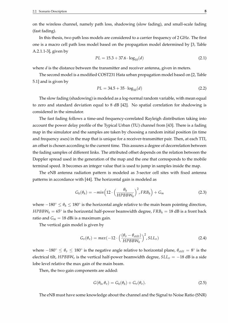
on the wireless channel, namely path loss, shadowing (slow fading), and small-scale fading
(fast fading).
In this thesis, two path loss models are considered to a carrier frequency of 2 GHz. The first
one is a macro cell path loss model based on the propagation model determined by [3, Table
A.2.1.1-3], given by
PL = 15.3 + 37.6 · log10(d) (2.1)
where d is the distance between the transmitter and receiver antenna, given in meters.
The second model is a modified COST231 Hata urban propagation model based on [2, Table
5.1] and is given by
PL = 34.5 + 35 · log10(d) (2.2)
The slow fading (shadowing) is modeled as a log-normal random variable, with mean equal
to zero and standard deviation equal to 8 dB [42]. No spatial correlation for shadowing is
considered in the simulator.
The fast fading follows a time-and frequency-correlated Rayleigh distribution taking into
account the power delay profile of the Typical Urban (TU) channel from [43]. There is a fading
map in the simulator and the samples are taken by choosing a random initial position (in time
and frequency axes) in the map that is unique for a receiver-transmitter pair. Then, at each TTI,
an offset is chosen according to the current time. This assures a degree of decorrelation between
the fading samples of different links. The attributed offset depends on the relation between the
Doppler spread used in the generation of the map and the one that corresponds to the mobile
terminal speed. It becomes an integer value that is used to jump in samples inside the map.
The eNB antenna radiation pattern is modeled as 3-sector cell sites with fixed antenna
patterns in accordance with [44]. The horizontal gain is modeled as
Gh(θh) = −min(
12 ·( θh
HPBBWh
)2, FRBh
)+ Gm (2.3)
where −180◦ ≤ θh ≤ 180◦ is the horizontal angle relative to the main beam pointing direction,
HPBBWh = 65◦ is the horizontal half-power beamwidth degree, FRBh = 18 dB is a front back
ratio and Gm = 18 dBi is a maximum gain.
The vertical gain model is given by
Gv(θv) = max(−12 ·( (θv − θetilt)
HPBBWh
)2, SLLv) (2.4)
where −180◦ ≤ θv ≤ 180◦ is the negative angle relative to horizontal plane, θetilt = 8◦ is the
electrical tilt, HPBBWv is the vertical half-power beamwidth degree, SLLv = −18 dB is a side
lobe level relative the max gain of the main beam.
Then, the two gain components are added:
G(θh, θv) = Gh(θh) + Gv(θv). (2.5)
The eNB must have some knowledge about the channel and the Signal to Noise Ratio (SNR)
2.2. Scenario Description 9
of its UE for each RB to be able to determine suitable receive and transmit filter and to perform
the scheduling. The instantaneous SNR γj,s of UE j in RB s at TTI n is given by
γj,s[n] =ps|hj,s|2
σ2 , (2.6)
where σ2 denotes the thermal noise power, which is considered constant for all UE.
In practice, the channel is estimated by the UE using pilot symbols transmitted by the eNB.
The estimated channel can be modeled according to the model described in [45]:
hj,s[n] =√
υ · hj,s[n] +√(1− υ) · η[n] (2.7)
where υ is a real number between (0, 1) that represents the quality of the channel estimation
(υ = 1 indicates perfect channel estimation); and η[n] models the channel estimation
error, modeled as a Zero Mean Circularly Symmetric Complex Gaussian (ZMCSCG) random
variable, with E|η[n]|2 = E|hj,s[n]|2.
All UE report in periods of θ TTIs and the eNB receives the measure delayed of ∆n TTIs.
The Channel State Information (CSI) used by the eNB is given by
hj,s[n] = hj,s[n− ∆n− (n mod δ)] (2.8)
In this thesis, we study the CSI imperfections regarding the delay of the measurements.
Hence, it is considered that the channels can be perfectly estimated (υ = 1) and that the reports
are performed at every TTI (δ = 1).
The Signal to Interference-plus-Noise Ratio (SINR) information available in the eNB is
Γj,s[n] =ps|hj,s[n]|2
Ij,s + σ2, (2.9)
where Ij,s is the estimation of the interference reported by each UE j to the eNB.
Since it is prohibitive to obtain information about all interference links, thus it is considered
that the UE can estimate the instantaneous total interference power, and filter these results
along ω TTIs. Interference is estimated regardless of the RBs and is smoothed using an
exponential moving average post-filter estimator, which has low complexity. Thus, the
estimation of the interference power reported by each UE j to its eNB can be written as
Ij,s[n] =(
1− 1ω
)Ij,s[n− 1] +
1ω
Ij,s[n] (2.10)
The transmission can fail due to bad channel conditions, wherein the whole information
block is lost. Considering ϕ[n] as a binary variable that equals 1 if the transmission fails and 0,
otherwise, the BLock Error Rate (BLER) is defined as
Pe =1
NS
N
∑k=1
∑j∈J
∑s∈S
ϕ[n] (2.11)
2.2. Scenario Description 10
−10 −5 0 5 10 15 20 25 300
0.1
0.2
0.3
0.4
0.5
0.6
0.7
0.8
0.9
1
SINR [dB]
BLE
R
MCS−1
MCS−2
MCS−3
MCS−4
MCS−5
MCS−6
MCS−7
MCS−8
MCS−9
MCS−10
MCS−11
MCS−12
MCS−13
MCS−14
MCS−15
(a) BLER.
−10 −5 0 5 10 15 20 250
0.1
0.2
0.3
0.4
0.5
0.6
0.7
0.8
0.9
1
SINR [dB]
Avera
ge t
hro
ugh
pu
t [k
ilobit
/s]
MCS−1
MCS−2
MCS−3
MCS−4
MCS−5
MCS−6
MCS−7
MCS−8
MCS−9
MCS−10
MCS−11
MCS−12
MCS−13
MCS−14
MCS−15
(b) Normalized average throughput.
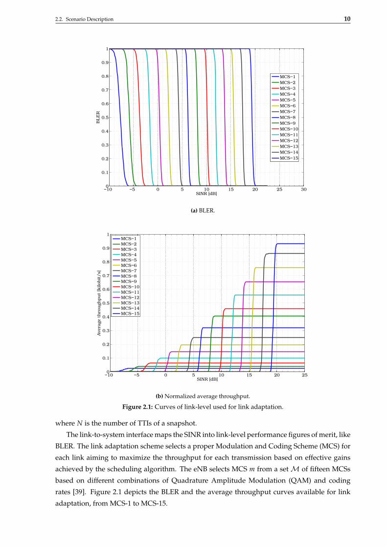
Figure 2.1: Curves of link-level used for link adaptation.
where N is the number of TTIs of a snapshot.
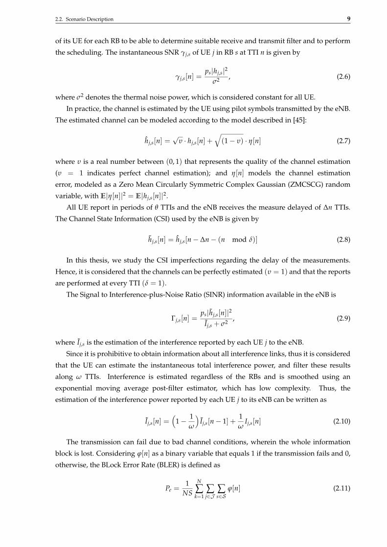
The link-to-system interface maps the SINR into link-level performance figures of merit, like
BLER. The link adaptation scheme selects a proper Modulation and Coding Scheme (MCS) for
each link aiming to maximize the throughput for each transmission based on effective gains
achieved by the scheduling algorithm. The eNB selects MCS m from a setM of fifteen MCSs
based on different combinations of Quadrature Amplitude Modulation (QAM) and coding
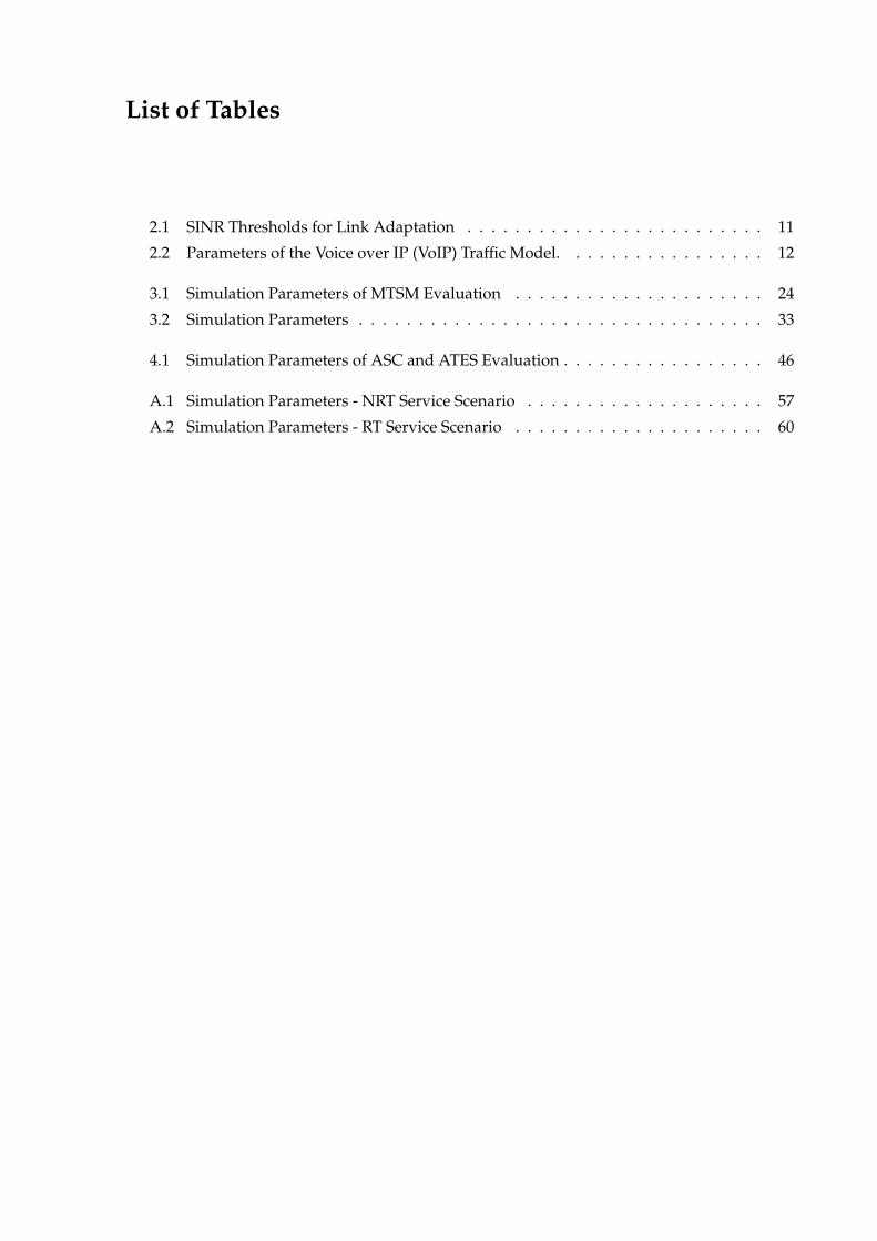
rates [39]. Figure 2.1 depicts the BLER and the average throughput curves available for link
adaptation, from MCS-1 to MCS-15.

2.2. Scenario Description 11
Table 2.1: SINR thresholds for link adaptation [46].
MCS Modulation Code rate [×1024] Rate [Bits/symbol] SINR threshold [dB]MCS-1 4-QAM 78 0.1523 −6.2MCS-2 4-QAM 120 0.2344 −5.6MCS-3 4-QAM 193 0.3770 −3.5MCS-4 4-QAM 308 0.6016 −1.5MCS-5 4-QAM 449 0.8770 0.5MCS-6 4-QAM 602 1.1758 2.5MCS-7 16-QAM 378 1.4766 4.6MCS-8 16-QAM 490 1.9141 6.4MCS-9 16-QAM 616 2.4062 8.3MCS-10 64-QAM 466 2.7305 10.4MCS-11 64-QAM 567 3.3223 12.2MCS-12 64-QAM 666 3.9023 14.1MCS-13 64-QAM 772 4.5234 15.9MCS-14 64-QAM 873 5.1152 17.7MCS-15 64-QAM 948 5.5547 19.7
The link adaptation interface selects the MCS that yields the maximum average throughput.
As defined in [43], a given MCS requires a certain SINR to operate with an acceptably low
BLER. By fixing a target desirable value of BLER, the minimum values can be achieved from the
link adaptation curves that ensure maintaining the required target BLER. Table 2.1 summarizes
the MCSs and their respective SINR thresholds. Observe that the lowest SINR value of −6.2
dB was determined in order to obtain a BLER of 1% on transmissions with MCS-1.
It is regarded different multi-antenna configurations for wireless links: Single Input Single
Output (SISO) and Multiple Input Single Output (MISO).
The application layer is the highest layer in the Open Systems Interconnection (OSI)
reference model. One important aspect of the application layer is the statistic nature of each
traffic type, which is emulated by a suitable traffic model. The traffic models are important for
the performance analysis of the network. Several traffic types are envisaged for evaluation
within the simulator each one with distinct characteristics. The services considered are
full-buffer traffic (Non-Real Time (NRT)) and VoIP (Real Time (RT)). The performance of
scheduling algorithms in OFDMA system depends on the considered traffic model.
The full buffer model simulates the worst case scenario, i.e., all users are greedy for
resources. The number of users in the cell is constant in each simulation snapshot and the
buffers of the users’ data flows always have unlimited amount of data to transmit [47]. The
full-buffer traffic is a simple and idealized traffic model where the transmit buffer associated
with each user has always data to be sent. This model is useful to simulate high loads since the
traffic associated to each user has 100% of activity.
The evaluation of RT services is based on the Voice over IP (VoIP) traffic model. It is a
conversational service that is an evolution of the old circuit-switched voice service. In this
service is assumed that a user within the cellular network is communicating with another user
outside the cellular network. The traffic model considers that an average voice activity of 50%
where speech and silence periods alternate following a two-state Markov chain depicted in
Figure 2.2.
In this figure, ζ and ξ are the transition probabilities from speech to silent and from silent
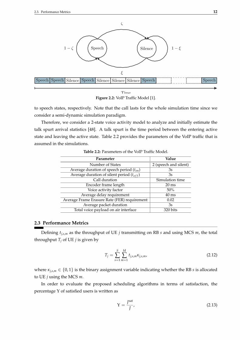
2.3. Performance Metrics 12
Speech
SpeechSpeechSpeechSpeechSpeech
Silence
SilenceSilenceSilenceSilence
ζ
1− ζ
ξ
1− ξ
TimeFigure 2.2: VoIP Traffic Model [1].
to speech states, respectively. Note that the call lasts for the whole simulation time since we
consider a semi-dynamic simulation paradigm.
Therefore, we consider a 2-state voice activity model to analyze and initially estimate the
talk spurt arrival statistics [48]. A talk spurt is the time period between the entering active
state and leaving the active state. Table 2.2 provides the parameters of the VoIP traffic that is
assumed in the simulations.
Table 2.2: Parameters of the VoIP Traffic Model.
Parameter ValueNumber of States 2 (speech and silent)
Average duration of speech period (ton) 3sAverage duration of silent period (to f f ) 3s
Call duration Simulation timeEncoder frame length 20 msVoice activity factor 50%
Average delay requirement 40 msAverage Frame Erasure Rate (FER) requirement 0.02
Average packet duration 3sTotal voice payload on air interface 320 bits
2.3 Performance Metrics
Defining tj,s,m as the throughput of UE j transmitting on RB s and using MCS m, the total
throughput Tj of UE j is given by
Tj =S
∑s=1
M
∑m=1
tj,s,mκj,s,m, (2.12)
where κj,s,m ∈ {0, 1} is the binary assignment variable indicating whether the RB s is allocated
to UE j using the MCS m.
In order to evaluate the proposed scheduling algorithms in terms of satisfaction, the
percentage Υ of satisfied users is written as
Υ =Jsat
J, (2.13)
2.4. Comparison Algorithms 13
where Jsat is the number of satisfied users in the cell. An NRT user is considered satisfied if its
session throughput is equal or higher than a threshold (Tj[n] ≥ Treqj ). An RT user is considered
satisfied if its FER is equal or lower than a threshold (dj[n] ≤ dreqj ). It is assumed that a frame is
lost if a packet arrives at the receiver later than the delay budget [26]. According to [48], a VoIP
user is considered not satisfied if 98% radio interface tail latency of the user is greater than 50
ms. This assumes an end-to-end delay below 200 ms for mobile-to-mobile communications.
The Jain’s index is used to evaluate the scheduling techniques in terms of fairness. For a
generic Quality of Service (QoS) metric x = [x1, · · · , xj, · · · , xJ ], Jain’s fairness index can be
written as
F(x) =
(∑J
j=1 xj
)2
J ·∑Jj=1 x2
j
, (2.14)
Jain’s fairness index is independent of scale and is bounded between 1/J and 1. A totally fair
allocation (with all xj’s equal) has fairness equal to 1, while a totally unfair allocation (with all
resources given to only one user), has fairness equal to 1/J. For NRT services, xj is given by
the throughput Tj[n]. For RT services, xj corresponds to the Head Of Line (HOL) delay.
2.4 Comparison Algorithms
The Rate Maximization (RM) [49] algorithm for OFDMA systems aims to maximize the sum
of data rates of the users subject to a maximum transmission power constraint. The user with
index j? is chosen to receive on resource s in TTI n if it satisfies
j? = arg maxj{tj,s}. (2.15)
This algorithm assigns each resource to the user that has the highest channel gain on it and,
therefore, it is a pure opportunistic policy.
The Proportional Fair (PF) scheduler performs a trade-off between fairness and
throughput [18].It tries to serve users with favorable radio conditions in order to provide a
high instantaneous throughput relative to their average throughput. The user with index j? is
chosen to receive on resource s in TTI n according to
j? = arg maxj
{tj,s[n]Tj[n]
}. (2.16)
The Modified Largest Weighted Delay First (MLWDF) [50] policy selects the users to receive
on resource s in TTI n according to
j? = arg maxj
{dhol
j [n]tj,s[n]Tj[n]
}. (2.17)
This resource allocator is specially suitable for RT services, since it regards the HOL packet
delay in its formulation.
The Urgency and Efficiency-based Packet Scheduling (UEPS) [51] algorithm is utility-based.
It uses the relative status of the current channel to the average one as an efficiency indicator of

2.5. Simulator Description 14
radio resource usage and the time utility as a urgency factor. For the UEPS criterion, the user
with index j? is chosen to receive on resource s on TTI n according to
j? = arg maxj
{∣∣∣U′(dholj [n])
∣∣∣ · tj,s[n]Tj[n]
}. (2.18)
more details about the utility function U are given in the next chapter.
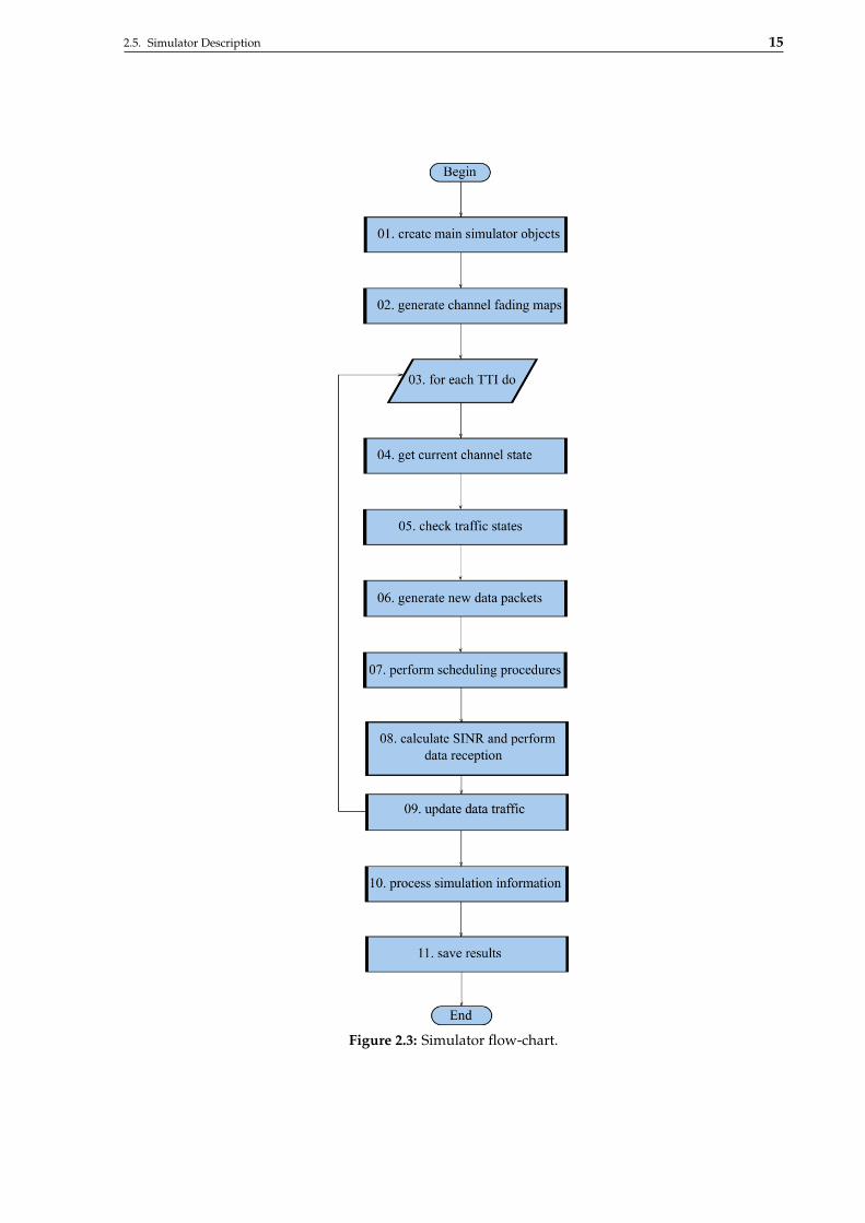
2.5 Simulator Description
This section presents the architecture of a semi-dinamic system-level simulator developed
to evaluate an OFDMA-based Radio Access Network (RAN). The simulator is composed
of three parts: initialization, main loop and results processing. In the initialization, all the
simulation objects and data structures are created, such as UE, eNB, cellular grid and channel
fading maps. In the main loop the simulation time is advanced and the state of simulation
parameters are updated according to the dynamics of the system. Finally, in the results
processing the simulation objects are processed in order to obtain statistics necessary to analyse
the system’s performance. Through the evaluation of these statistics the system performance
can be optimized by the proposal of new RRM strategies.
Figure 2.3 depicts the main elements of the simulation. In the beginning of the flow-chart,
there are the steps 01 and 02 that create the simulator objects (e.g., the set of UE J =
{1, 2, · · · , J} ) and generate the channel fading map (hj,s). The steps inside the main loop (04 to
09) are the core of the simulator. The essential tasks performed are:
I step 04: take the channel state and CSI available at the transmitter and receiver to provide
fundamental information to scheduling procedures, perform data reception and verify if
there were errors in the received data packets;
I steps 05− 06: check traffic state aiming to evaluate if new packects should be generated.
The packet size and packet generation frequency depends of the type of service, like NRT
or RT;
I step 07: exploiting the available information of channel and traffic, the scheduling
algorithm define the distribution of resources according to QoS requirements;
I step 08: after the assignment of resources, the data reception is performed to evaluate if
the data packets were successfully transmitted; the received SINR is calculated according
to (2.9) and mapped to the link-to-system curves to estimate packet error probabilities;
I step 09: according to the amount of data that was correctly received, the transmitter buffer
of the eNB with respect to each connected UE is updated.
Finally, step 10 processes and step 11 saves the simulation data in order to obtain statistics
that will be useful to analyse the system performance.
2.5. Simulator Description 15
Figure 2.3: Simulator flow-chart.
Chapter 3Scheduling Framework to Improve User
Satisfaction
In this chapter, the problem of maximizing the user satisfaction is investigated. Section 3.1
presents the general optimization formulation and the utility-based scheduling framework.
Section 3.2 details the studied algorithms, describing the different utility functions considered
to develop the framework. Sections 3.3 and 3.4 evaluate the proposed algorithms and
Section 3.5 provides a partial conclusion based on the observed performance results.
3.1 General Utility-Based Scheduling Framework
Utility theory allows to connect the Physical Layer (PHY) and the Medium Access Control
(MAC) sublayer to achieve cross-layer optimization [19]. This theory is a flexible tool to deal
with different trade-offs, like capacity versus fairness or capacity versus satisfaction.
In this study, we consider a general scheduling framework that is able to maximize the
degree to which a network satisfies service requirements of users’ applications in terms of
throughput and delay. The general optimization problem is formulated as
maxSj
J
∑j=1
U(xj[n]
), (3.1a)
subject toJ⋃
j=1
Sj ⊆ S , (3.1b)
Si⋂Sj = ∅, i 6= j, ∀i, j ∈ {1, . . . , J}, (3.1c)
where S is the set of all resources in the system, J is the total number of User Equipment (UE),
Sj is the subset of resources assigned to the UE j, and U(xj[n]
)is a utility function based on a
generic Quality of Service (QoS) metric xj[n] measured in the Transmission Time Interval (TTI)
n.
The constraints (3.1b) and (3.1c) state that the union of all subsets of resources allocated to
different users must be limited to the total set of resources available in the system and that the
same resource cannot be shared by two or more users in the same TTI, respectively.
It is demonstrated in [20] that a simplified optimization problem can be derived from the
3.1. General Utility-Based Scheduling Framework 17
original one given by (3.1). According to this simplification, the objective function of (3.1)
becomes linear in terms of the instantaneous user’s data rate and the problem is characterized
as a weighted sum rate maximization, whose weights are adaptively controlled by the marginal
utilities. The objective function of the simplified problem is given by
maxSj
J
∑j=1
U′(xj[n]) · Rj[n], (3.2)
where Rj[n] is the instantaneous data rate of UE j and U′(xj) is the first derivative of the utility
function of the UE j with respect to the QoS metric.
The study in [20] established that if we consider a fixed power allocation, the scheduling is
based on the selection of the user with index j? to receive on the resource s in TTI n according
to
j? = arg maxj
{wj · rj,s [n]
}, (3.3)
where wj is the utility-based weight of UE j and rj,s is the instantaneous achievable transmission
rate of user j with respect to Resource Block (RB) s ∈ S .
This work aims to formulate general scheduling algorithms suitable for maximizing the
satisfaction of different types of services. Therefore, the variable xj can be either the users’
average data rates (throughput) or the users’ Head Of Line (HOL) packet delay, which are QoS
metrics suitable for Non-Real Time (NRT) and Real Time (RT) services, respectively.
In the one hand, if the UE j has NRT service, the marginal utility is given by
wNRTj =
∂U∂Tj
∣∣∣Tj=Tj[n−1]
(3.4)
where Tj[n− 1] is the average throughput of UE j calculated up to the previous TTI, i.e., TTI
n− 1. On the other hand, if j has a RT service, the marginal utility is obtained by
wRTj =
∣∣∣ ∂U∂dHOL
j
∣∣∣dHOL
j [n]=dHOLj [n]
∣∣∣, (3.5)
where dHOLj is the HOL packet delay of UE j in the TTI n.
Therefore, the utility-based weights (3.4) and (3.5) provide sufficient information to allocate
the resources to the users leading to a QoS-based scheduling with low complexity. In fact,
all necessary computations to allocate resources according to these equations are simple
operations:
i. calculation of the marginal utility per user,
ii. calculation of the product between the marginal utility per user and instantaneous data
rate, and
iii. sorting the users by this product value in (3.3) on each resource.
If more than one user has the same priority, a tiebreaker process selects the user with the highest
Signal to Noise Ratio (SNR).

3.2. Maximization of User Satisfaction Using Suitable Utility Functions 18
Figure 3.1: Utility-based scheduling algorithm flow-chart.
Figure 3.1 depicts the utility-based scheduling procedure mentioned on the simulator
flow-chart described on Chapter 2.
3.2 Maximization of User Satisfaction Using Suitable Utility Functions
3.2.1 TSM/DSM Based on the Logistic Function
The authors of [26] proposed two utility-based scheduling algorithms able to maximize
the number of satisfied users in a 4th Generation (4G) cellular system. The first one is the
Throughput-based Satisfaction Maximization (TSM) algorithm , whose formulation is based
on the users’ throughput and which is suitable for NRT services. The second one is the
Delay-based Satisfaction Maximization (DSM) algorithm, whose formulation is based on the
users’ HOL packet delay and which is suitable for RT services.
The TSM and DSM algorithms originally used a sigmoid utility function based on a generic
QoS metric xj[n] of the UE j. In this work, the sigmoid is written as the logistic function. This
change wants to consider a function continuously differentiable over the interval of xj[n] and
limited between 0 and 1. The logistic function is given by
ULo(x?j [n]) =1
1 + eµ(x?j [n]−x?reqj )/σ
, (3.6)
where x?j is the current QoS metric; σ is a nonnegative parameter that sets the shape of the
logistic function and µ is a constant which determines if the function is ascending (µ = −1) or
3.2. Maximization of User Satisfaction Using Suitable Utility Functions 19
descending (µ = 1).
Without loss of generality, it is established that xj is normalized by the QoS requirement.
Considering NRT services xj = T?j /T?req
j and Treqj = T?req
j /T?reqj = 1. Considering RT services,
it is established that xj = d?j /d?reqj and dreq
j = d?reqj /d?req
j = 1. Therefore, ULog(x?j [n]) is simply
replaced by ULog(xj[n]) hereafter.
The TSM algorithm employs an increasing step-shaped utility curve centered at xreqj . As
indicated on Figure 3.2(a) by the solid line, a user becomes satisfied rapidly if its throughput
approaches the requirement. The opposite occurs when the user throughput decreases to
values lower than the requirement. This behavior is in accordance with the definition of
satisfaction for NRT services generally found in the literature [26].
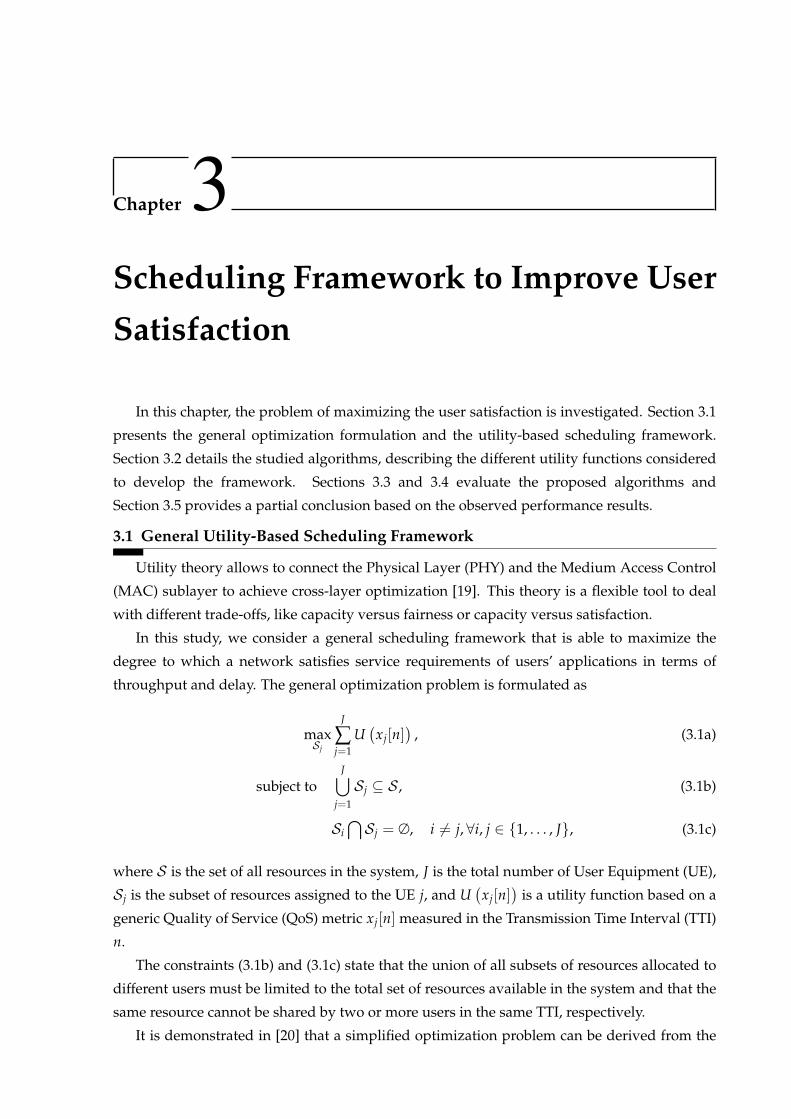
The DSM algorithm employs a decreasing step-shaped function, as indicated on
Figure 3.2(a) by the dashed line. A given user becomes unsatisfied rapidly if the HOL packet
delay approaches or exceeds the delay requirement. The opposite occurs when the user delay
decreases to values below the requirement.
In this study, we establish that the logistic is equal to a given value δ when the QoS metric
xj achieves a proportion ρ of the QoS requirement xreqj . Therefore, the shape parameter of the
logistic function is given by
σ =µ · (ρ− 1) · xreq
j
log(
1δ− 1) . (3.7)
Regarding the NRT utility function, we achieved satisfactory results when δ = 0.01, ρ =
0.50 and xreqj = 1. The NRT function starts to increase noticeably, i.e., U(xj) = δ = 0.01,
when xj is half of the QoS requirement, i.e., xj = ρ · xreqj = 0.50. Using (3.7), we have that
σTSM = 0.1088. For the case of RT services, the utility function starts to decrease noticeably, i.e.,
Uj(xj) = 0.99, when xj is half of the QoS requirement, i.e., xj = ρ · xreqj = 0.50. Using (3.7),
we also obtained σDSM = 0.1088. Figure 3.2(a) shows the curves obtained using this strategy to
determine the parameter adjustment.
The utility-based weight performs an important function in the scheduling algorithm, once
Normalized QoS Metric
0 0.25 0.50 0.75 1.00 1.25 1.50 1.75 2.00
Uti
lity
0
0.2
0.4
0.6
0.8
1
TSM Algorithm
δ = 0.01
µ = −1
ρ = 0.50
DSM Algorithm
δ = 0.99
µ = 1
ρ = 0.50
(a) Utility functions
Normalized QoS Metric
0 0.25 0.50 0.75 1.00 1.25 1.50 1.75 2.00
Mar
gin
al U
tili
ty
0
0.5
1
1.5
2
2.5
(b) Marginal utility function
Figure 3.2: Original curves of TSM and DSM algorithms using the parameter adjustment described by(3.7).
3.2. Maximization of User Satisfaction Using Suitable Utility Functions 20
the priority of a given user to get a resource is directly proportional to this weight. The
utility-based weight in (3.3), based on a generic QoS metric xj of the UE j, is given by the
marginal utility, which is the first derivative of the utility function U(xj[n]) with respect to the
QoS metric xj[n], i.e., wj =∂U(xj[n])
∂xj[n]. Therefore, the logistic marginal utility is given by
wLoj =
µeµ(xj[n]−xreqj )/σ
σ(1 + eµ(xj[n]−xreqj )/σ)2
. (3.8)
The particular expression of wLoj must be used in the corresponding scheduler algorithm
given by (3.3). The marginal utility represented by (3.8) is a bell-shaped function, which is
a symmetric function centralized at the xreqj = 1. Figure 3.2(b) indicates the marginal utility
function achieved with this parametrization. Since we use normalized values of xj and the
adjustment of the parameter results in the same value σ = 0.1088 for RT and NRT services,
the utility-based weight curve is equal for TSM and DSM algorithms. The users who have a
higher priority in the scheduling process are the ones experiencing QoS levels close to the QoS
requirement.
The study performed in [26] demonstrates that it is possible to provide high user satisfaction
for NRT and RT users with low complexity if we consider the logistic function as the utility
function in the scheduling. The present work extends the utility-based framework, employing
a new utility function, called shifted log-logistic, which has more parameters and provides
conditions to manage the resources more efficiently.
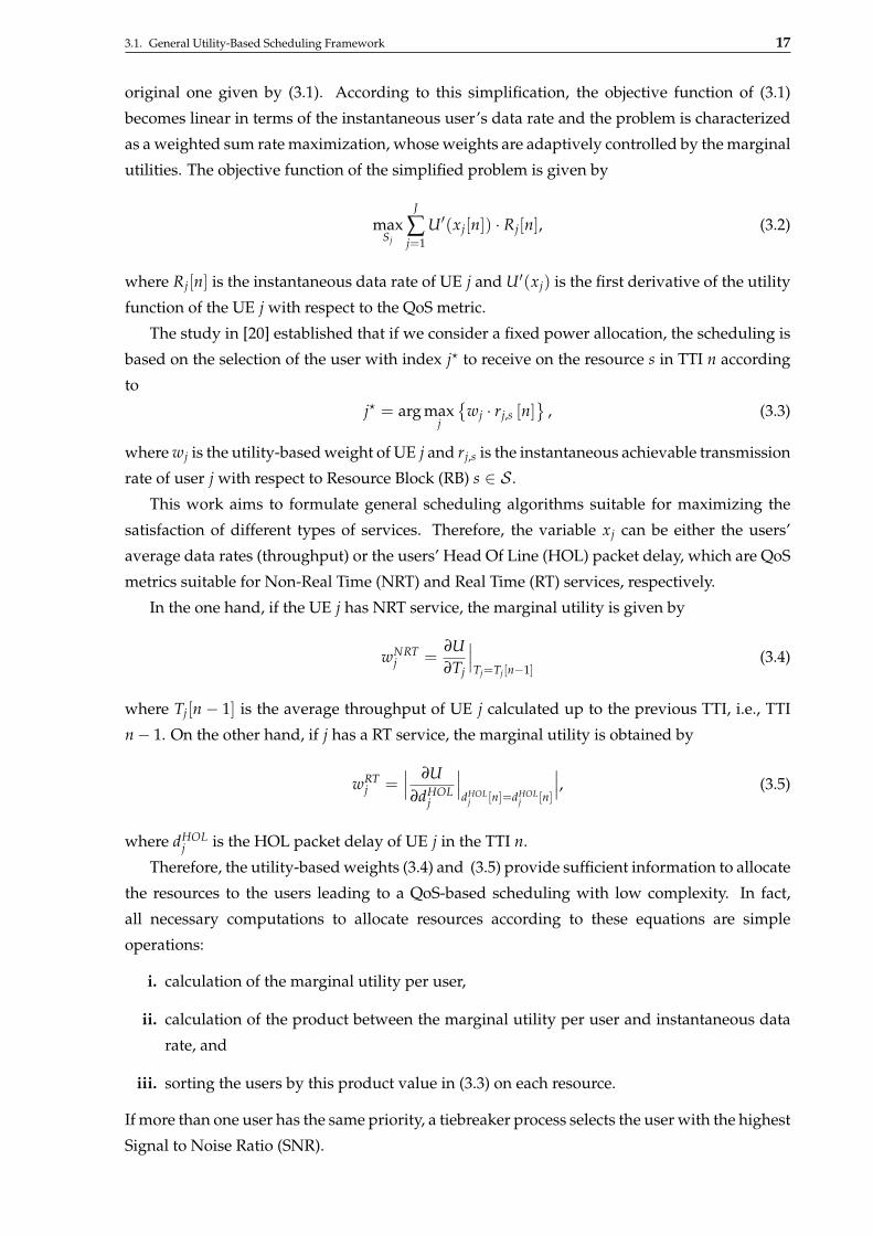
3.2.2 MTSM/MDSM Based on the Shifted Log-Logistic Utility Function
Utility functions are used to solve scheduling optimization problems for different
applications, building a bridge among several layers of the wireless communication system
[19]. Previous studies employed different utility functions, like exponential and logarithm [52].
After an extensive research of utility functions with different properties, like laplace, cauchy,
dirichlet, beta [53], the author achieved interesting results with the shifted log-logistic utility
function, a continuously differentiable function of the QoS metric xj, represented by
US-Log(xj[n]) =1
1 +(
1 +θη
λ(xj[n]− xreq
j )
)−1/θ, (3.9)
where xj[n] is the normalized QoS metric and xreqj is the QoS requirement of the UE j; θ is a real
parameter which determines the shape of the curve; λ is a real parameter that sets the scale of
the function; and η is a constant which asserts if the function is ascending (η = 1) or descending
(η = −1).
According to the value of the shape parameter θ, the shifted log-logistic utility function is
determined at different xj[n] intervals:
i. xj[n] ≥ xreqj −
λ
θ, if θ > 0;
ii. xj[n] ∈ (−∞, ∞), if θ = 0;
3.2. Maximization of User Satisfaction Using Suitable Utility Functions 21
iii. xj[n] ≤ xreqj −
λ
θ, if θ < 0.
Exploiting the properties of the shifted log-logistic utility function, the new scheduling
schemes called Modified Throughput-based Satisfaction Maximization (MTSM) and Modified
Delay-based Satisfaction Maximization (MDSM) are able to deal with the scheduling more
efficiently, giving more flexibility to the framework and making possible to improve of the
user satisfaction for NRT and RT services, respectively.
It is important to consider the reasons of the choice of the shifted log-logistic utility function.
Firstly, this function is continuously differentiable over the range xj[n] and limited between 0
and 1, i.e., 0 ≤ US-Log ≤ 1. Secondly, it has two parameters, θ and λ that clearly impact its
behavior, allowing different Radio Resource Allocation (RRA) strategies to be configured by a
suitable parameter setting, as it will be shown in this study.
The MTSM algorithm employs an increasing step-shaped utility curve centered at Treqj . This
behavior is in conformity with the definition of satisfaction for NRT services used previously in
the TSM algorithm: a user is quickly satisfied if its throughput approaches to the requirement;
or its satisfaction decreases to lower values when distant from the requirement. However, this
new function has a different range of variation in comparison with the original sigmoid, as
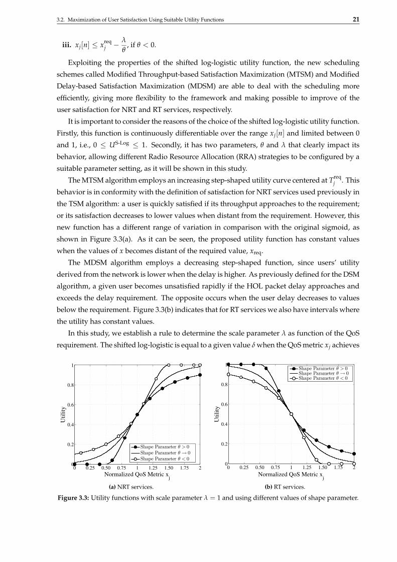
shown in Figure 3.3(a). As it can be seen, the proposed utility function has constant values
when the values of x becomes distant of the required value, xreq.
The MDSM algorithm employs a decreasing step-shaped function, since users’ utility
derived from the network is lower when the delay is higher. As previously defined for the DSM
algorithm, a given user becomes unsatisfied rapidly if the HOL packet delay approaches and
exceeds the delay requirement. The opposite occurs when the user delay decreases to values
below the requirement. Figure 3.3(b) indicates that for RT services we also have intervals where
the utility has constant values.
In this study, we establish a rule to determine the scale parameter λ as function of the QoS
requirement. The shifted log-logistic is equal to a given value δ when the QoS metric xj achieves
0 0.25 0.50 0.75 1 1.25 1.50 1.75 20
0.2
0.4
0.6
0.8
1
Normalized QoS Metric xj
Uti
lity
Shape Parameter θ > 0
Shape Parameter θ → 0
Shape Parameter θ < 0
(a) NRT services.
0 0.25 0.50 0.75 1 1.25 1.50 1.75 20
0.2
0.4
0.6
0.8
1
Normalized QoS Metric xj
Uti
lity
Shape Parameter θ > 0Shape Parameter θ → 0Shape Parameter θ < 0
(b) RT services.
Figure 3.3: Utility functions with scale parameter λ = 1 and using different values of shape parameter.
3.2. Maximization of User Satisfaction Using Suitable Utility Functions 22
a proportion ρ of the QoS requirement xreqj . Therefore, the scale parameter is given by
λ =θηxreq
j (ρ− 1)(δ
1− δ
)θ
− 1
. (3.10)
Considering the NRT utility function, satisfactory results have been achieved when the
curve starts to increase noticeably, i.e., Uj(xj) = δ = 0.01, when xj is half of the QoS
requirement, i.e., xj = ρ · xreqj = 0.50. Using θ → 0 in (3.10), follows that λMTSM = 0.1088.
Regarding RT services, the utility function starts to decrease significantly, i.e., Uj(xj) = 0.99,
when xj is half of the QoS requirement, i.e., xj = ρ · dreqj = 0.50. Using θ → 0 in (3.10), is
obtained that λMDSM = 0.1088.
The shifted log-logistic function has the marginal utility given by
wS-Logj =
η
λ
(1 +
θη
λ(xj[n]− xreq
j ))−1−1/θ
(1 +
(1 +
θη
λ(xj[n]− xreq
j ))−1/θ)2 . (3.11)
It is important to observe that the shifted log-logistic is a generalization of the logistic
function, since wS-Logj → wLo
j when θ → 0. More details are provided in Appendix B.
The format of marginal utility functions impacts the scheduling algorithms, determining
suitable arrangements to improve the users’ satisfaction. For comparison purposes and
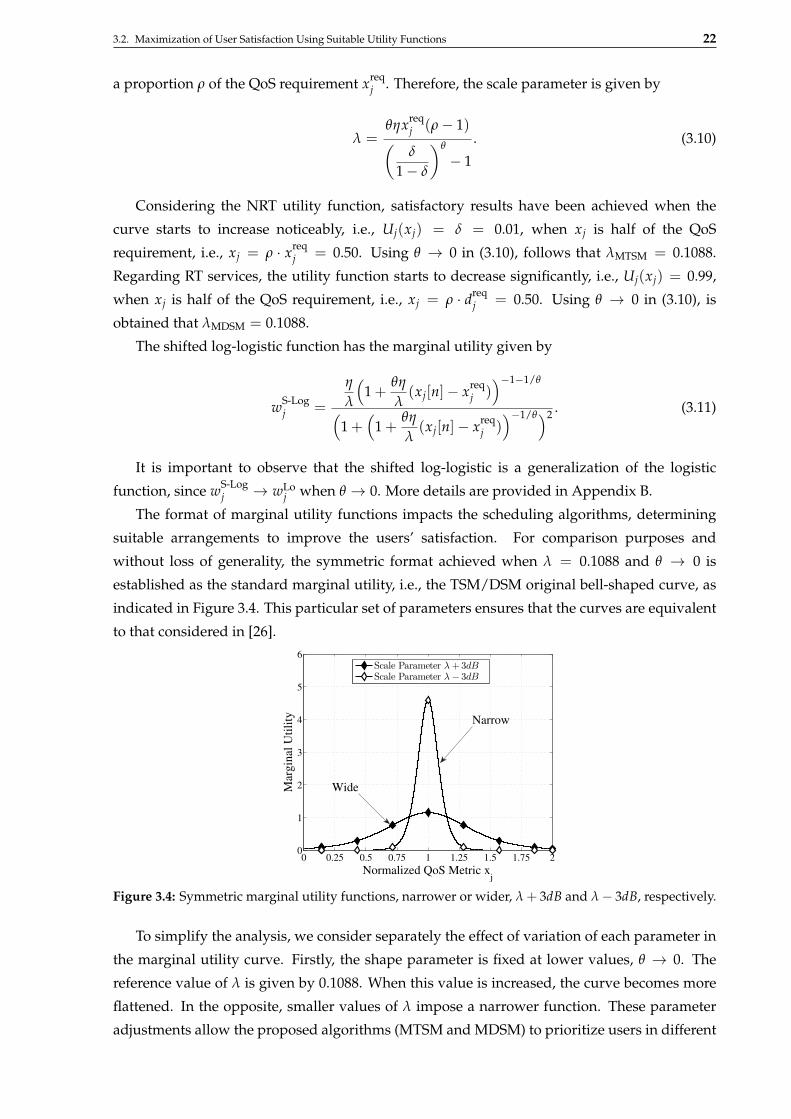
without loss of generality, the symmetric format achieved when λ = 0.1088 and θ → 0 is
established as the standard marginal utility, i.e., the TSM/DSM original bell-shaped curve, as
indicated in Figure 3.4. This particular set of parameters ensures that the curves are equivalent
to that considered in [26].
0 0.25 0.5 0.75 1 1.25 1.5 1.75 20
1
2
3
4
5
6
Normalized QoS Metric xj
Mar
gin
al U
tili
ty
Scale Parameter λ+3dB
Scale Parameter λ− 3dB
Wide
Narrow
Figure 3.4: Symmetric marginal utility functions, narrower or wider, λ + 3dB and λ− 3dB, respectively.
To simplify the analysis, we consider separately the effect of variation of each parameter in
the marginal utility curve. Firstly, the shape parameter is fixed at lower values, θ → 0. The
reference value of λ is given by 0.1088. When this value is increased, the curve becomes more
flattened. In the opposite, smaller values of λ impose a narrower function. These parameter
adjustments allow the proposed algorithms (MTSM and MDSM) to prioritize users in different
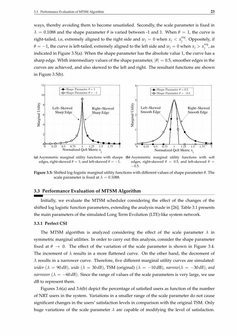
3.3. Performance Evaluation of MTSM Algorithm 23
ways, thereby avoiding them to become unsatisfied. Secondly, the scale parameter is fixed in
λ = 0.1088 and the shape parameter θ is varied between -1 and 1. When θ = 1, the curve is
right-tailed, i.e, extremely aligned to the right side and wj = 0 when xj < xreqj . Oppositely, if
θ = −1, the curve is left-tailed, extremely aligned to the left side and wj = 0 when xj > xreqj , as
indicated in Figure 3.5(a). When the shape parameter has the absolute value 1, the curve has a
sharp edge. Whth intermediary values of the shape parameter, |θ| = 0.5, smoother edges in the
curves are achieved, and also skewed to the left and right. The resultant functions are shown
in Figure 3.5(b).
0 0.25 0.5 0.75 1 1.25 1.5 1.75 20
2
4
6
8
10
12
Normalized QoS Metric xj
Mar
gin
al U
tili
ty
Shape Parameter θ = 1
Shape Parameter θ =−1
Left−SkewedSharp Edge
Right−SkewedSharp Edge
(a) Asymmetric marginal utility functions with sharpeedges, right-skewed θ = 1; and left-skewed θ = −1.
0 0.25 0.5 0.75 1 1.25 1.5 1.75 20
1
2
3
4
Normalized QoS Metric xj
Mar
gin
al U
tili
ty
Shape Parameter θ = 0.5
Shape Parameter θ =−0.5
Right−SkewedSmooth Edge
Left−SkewedSmooth Edge
(b) Asymmetric marginal utility functions with softedges, right-skewed θ = 0.5, and left-skewed θ =−0.5.
Figure 3.5: Shifted log-logistic marginal utility functions with different values of shape parameter θ. Thescale parameter is fixed at λ = 0.1088.
3.3 Performance Evaluation of MTSM Algorithm
Initially, we evaluate the MTSM scheduler considering the effect of the changes of the
shifted log logistic function parameters, extending the analysis made in [26]. Table 3.1 presents
the main parameters of the simulated Long Term Evolution (LTE)-like system network.
3.3.1 Perfect CSI
The MTSM algorithm is analyzed considering the effect of the scale parameter λ in
symmetric marginal utilities. In order to carry out this analysis, consider the shape parameter
fixed at θ → 0. The effect of the variation of the scale parameter is shown in Figure 3.4.
The increment of λ results in a more flattened curve. On the other hand, the decrement of
λ results in a narrower curve. Therefore, five different marginal utility curves are simulated:
wider (λ = 90 dB), wide (λ = 30 dB), TSM (original) (λ = −10 dB), narrow(λ = −30 dB), and
narrower (λ = −60 dB). Since the range of values of the scale parameters is very large, we use
dB to represent them.
Figures 3.6(a) and 3.6(b) depict the percentage of satisfied users as function of the number
of NRT users in the system. Variations in a smaller range of the scale parameter do not cause
significant changes in the users’ satisfaction levels in comparison with the original TSM. Only
huge variations of the scale parameter λ are capable of modifying the level of satisfaction.
3.3. Performance Evaluation of MTSM Algorithm 24
Table 3.1: Simulation Parameters of MTSM Evaluation
Parameter ValueMaximum BS transmit power 20 WBS antenna radiation pattern Three-sectoredCell radius 1 kmUE speed 3 km/hCarrier frequency 2 GHzSystem bandwidth 5 MHzSub-carrier bandwidth 15 kHzNumber of RBs 25 NRTPath loss - macro cell scenario [3] PL = 15.3 + 37.6 · log10(d)
a
Path loss - urban macro scenario [2] PL = 34.5 + 35 · log10(d)a
Channel coherence time 90 msAntenna gainb[44] Gh(θh) + Gv(θv)Downtilt angle 8 degreesLog-normal shadowing st. dev. 8 dBSmall-scale fading [43] 3GPP Typical UrbanAWGN power per sub-carrier -123.24 dBmNoise figure 9 dBLink adaptation Link level curves from [39]SNR threshold of MCS 1 [39] -6.9 dBTransmission Time Interval 1 msNRT traffic model Full bufferUser throughput requirement 512 kbpsMulti-antenna configuration SISOSimulation time span 10 sNumber of simulation runs 50Confidence Interval 95%a d is the distance to the BS in km.b θh and θv represent the horizontal and vertical angles related to
the Base Station (BS), respectively.
However wider and narrower curves cannot achieve gains. Oppositely, these modifications of
λ resulted in reductions of the satisfaction levels. This behavior occurs because the values of
marginal utility of the users distant of the requirement became of the same order, consequently
the scheduling of resources is determined by channel conditions, only the users with the higher
instantaneous rates are chosen.
Different channel propagation conditions are considered, a macro cell scenario [3] and an
urban macro scenario [2]. As expected, there are impacts on the satisfaction levels achieved
by the different algorithm configurations. The worsening of channel conditions decreases the
satisfaction levels and the proposed MTSM algorithm is more impacted than TSM. They start
from a tie situation in Figure 3.6(a) to a difference of 20% in Figure 3.6(b).
Figures 3.6(c) and 3.6(d) show the system capacity in terms of total throughput as a function
of the number of NRT users. A small increase of scale parameter λ provides a gain for
lower loads that disappears with the increasing number of users, as it can be seen in the
wide curve. The wider curve, which is achieved with a huge value of λ, has a flat marginal
utility function, and consequently users have utility weights of approximately the same order.
Since the scheduling also depends on the instantaneous data rate, this factor becomes more
significant than the marginal utility in the allocation process, which tends to a less equitable
distribution of resources, concentrating them with the users with best radio link quality.
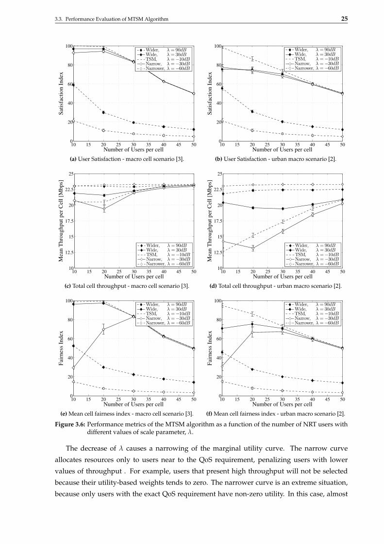
3.3. Performance Evaluation of MTSM Algorithm 25
10 15 20 25 30 35 40 45 500
20
40
60
80
100
Number of Users per cell
Sat
isfa
ctio
n I
nd
ex
Wider, λ = 90dBWide, λ = 30dBTSM, λ =−10dBNarrow, λ =−30dBNarrower, λ =−60dB
(a) User Satisfaction - macro cell scenario [3].
10 15 20 25 30 35 40 45 500
20
40
60
80
100
Number of Users per cell
Sat
isfa
ctio
n I
nd
ex
Wider, λ = 90dBWide, λ = 30dBTSM, λ =−10dBNarrow, λ =−30dBNarrower, λ =−60dB
(b) User Satisfaction - urban macro scenario [2].
10 15 20 25 30 35 40 45 5010
12.5
15
17.5
20
22.5
25
Number of Users per cell
Mea
n T
hro
ug
hp
ut
per
Cel
l [M
bp
s]
Wider, λ = 90dBWide, λ = 30dBTSM, λ =−10dBNarrow, λ =−30dBNarrower, λ =−60dB
(c) Total cell throughput - macro cell scenario [3].
10 15 20 25 30 35 40 45 5010
12.5
15
17.5
20
22.5
25
Number of Users per cell
Mea
n T
hro
ug
hp
ut
per
Cel
l [M
bp
s]
Wider, λ = 90dBWide, λ = 30dBTSM, λ =−10dBNarrow, λ =−30dBNarrower, λ =−60dB
(d) Total cell throughput - urban macro scenario [2].
10 15 20 25 30 35 40 45 500
20
40
60
80
100
Number of Users per cell
Fai
rnes
s In
dex
Wider, λ = 90dBWide, λ = 30dBTSM, λ =−10dBNarrow, λ =−30dBNarrower, λ =−60dB
(e) Mean cell fairness index - macro cell scenario [3].
10 15 20 25 30 35 40 45 500
20
40
60
80
100
Number of Users per cell
Fai
rnes
s In
dex
Wider, λ = 90dBWide, λ = 30dBTSM, λ =−10dBNarrow, λ =−30dBNarrower, λ =−60dB
(f) Mean cell fairness index - urban macro scenario [2].
Figure 3.6: Performance metrics of the MTSM algorithm as a function of the number of NRT users withdifferent values of scale parameter, λ.
The decrease of λ causes a narrowing of the marginal utility curve. The narrow curve
allocates resources only to users near to the QoS requirement, penalizing users with lower
values of throughput . For example, users that present high throughput will not be selected
because their utility-based weights tends to zero. The narrower curve is an extreme situation,
because only users with the exact QoS requirement have non-zero utility. In this case, almost
3.3. Performance Evaluation of MTSM Algorithm 26
all users are tied and the tiebreaker is based on the SNR. Therefore, the scheduling algorithm
is similar to Rate Maximization (RM).
As mentioned in the discussion of the results of satisfaction, the system capacity also is
impacted by the channel propagation conditions. The configurations with extreme values of
scale parametes (wider and narrower) suffer little impact since these settings schedule users
with the best conditions. But the other configurations (wide and narrow) are clearly more
affected, with a decrement of 50% of the mean throughput per cell for small loads from
Figure 3.6(c) to 3.6(d).
The fairness of the TSM algorithm followed the behavior observed for the satisfaction levels,
as it can be seen in Figure 3.6(e) and 3.6(f). As verified for the other metrics, there is a decrement
with the change of channel condition from macro cell scenario [3] to urban macro scenario [2].
The wider and narrower configurations of MTSM are little affected, maintaining low values
compared with the other ones. The configuration with λ = −30dB (narrow) distributes
resources to users near to the requirement. With a small number of users this results in an
uneven distribution of resources that is reduced with the increment of the system load. This
behavior can be observed in both propagation scenarios.
Therefore, the results showed that the modification of the scale parameter λ of the shifted
log-logistic utility function (i.e., symmetric marginal utility curves) allows the observation
of different behaviors of the scheduling algorithm , however it is not able to provide an
improvement of the satisfaction index of the system in comparison with the original TSM
algorithm.
From now on, we analyze the effect of the change of the shape parameter θ of the marginal
utility function given by (3.11). Positive values of the shape parameter, θ > 0, result in a
curve with the tail directed to the right side. In the opposite, negative values θ < 0 imply in
a tail directed to the left side. The magnitude of the scale parameter, θ, also determines the
behavior of the function when the values are near the QoS requirement: higher values of the
shape parameter, |θ| = 1, result in curves with sharper edges; lower values, |θ| = 0.5, imply in
smoother peaks.
TSM uses a symmetric bell-shaped curve according to Figure 3.2(b). The scale parameter
is fixed at λ = 0.1088. The simulated configurations of MTSM are given by the curves shown
in the Figures 3.5(a) and 3.5(b). Thus, five different marginal utility curves are analyzed: right
skewed with sharp edge (θ = 1), right skewed with soft edge (θ = 0.5), bell-shaped (θ → 0),
left skewed with soft edge (θ = −0.5), left skewed with sharp edge (θ = −1).
Figures 3.7(a) and 3.7(a) depict the percentage of satisfied users as a function of the
number of NRT users in the system. The symmetric configuration (TSM) avoids the users
to become unsatisfied because it gives the same priority to users with QoS levels just above
or just below the QoS requirement. The asymmetric curves give different priority to such
users. That difference in the distribution of priorities allows us to obtain an increase in the
satisfaction levels. While right skewed curves benefit users with the highest throughputs,
left skewed ones benefit users with throughput below the requirement. The highest gains in
the satisfaction levels are achieved with the left skewed configurations, hence giving more

3.3. Performance Evaluation of MTSM Algorithm 27
resources to users with low throughput improves their condition to get resources. The right
skewed and symmetric configurations have similar users’ satisfaction behavior, since they
benefit users with the best channel conditions.
10 15 20 25 30 35 40 45 5020
30
40
50
60
70
80
90
100
Number of Users per cell
Sat
isfa
ctio
n I
nd
ex
Right Skewed - Sharp Edge, θ = 1.00Right Skewed - Soft Edge, θ = 0.50TSM, θ → 0Left Skewed - Soft Edge, θ =−0.50Left Skewed - Sharp Edge, θ =−1.00
(a) User Satisfaction - macro cell scenario [3].
10 15 20 25 30 35 40 45 5020
30
40
50
60
70
80
90
100
Number of Users per cell
Sat
isfa
ctio
n I
nd
ex
Right Skewed - Sharp Edge, θ = 1.00Right Skewed - Soft Edge, θ = 0.50TSM, θ → 0Left Skewed - Soft Edge, θ =−0.50Left Skewed - Sharp Edge, θ =−1.00
(b) User Satisfaction - urban macro scenario [2].
10 15 20 25 30 35 40 45 500
2.5
5
7.5
10
12.5
15
17.5
20
22.5
25
Number of Users per cell
Mea
n T
hro
ug
hp
ut
per
Cel
l [M
bp
s]
Right Skewed - Sharp Edge, θ = 1.00Right Skewed - Soft Edge, θ = 0.50TSM, θ → 0Left Skewed - Soft Edge, θ =−0.50Left Skewed - Sharp Edge, θ =−1.00
(c) Total cell throughput - macro cell scenario [3].
10 15 20 25 30 35 40 45 500
2.5
5
7.5
10
12.5
15
17.5
20
22.5
25
Number of Users per cell
Mea
n T
hro
ug
hp
ut
per
Cel
l [M
bp
s]
Right Skewed - Sharp Edge, θ = 1.00Right Skewed - Soft Edge, θ = 0.50TSM, θ → 0Left Skewed - Soft Edge, θ =−0.50Left Skewed - Sharp Edge, θ =−1.00
(d) Total cell throughput - urban macro scenario [2].
10 15 20 25 30 35 40 45 500
10
20
30
40
50
60
70
80
90
100
Number of Users per cell
Fai
rnes
s In
dex
Right Skewed - Sharp Edge, θ = 1.00Right Skewed - Soft Edge, θ = 0.50TSM, θ → 0Left Skewed - Soft Edge, θ =−0.50Left Skewed - Sharp Edge, θ =−1.00
(e) Mean cell fairness index - macro cell scenario [3].
10 15 20 25 30 35 40 45 500
20
40
60
80
100
Number of Users per cell
Fai
rnes
s In
dex
Right Skewed - Sharp Edge, θ = 1.00Right Skewed - Soft Edge, θ = 0.50TSM, θ → 0Left Skewed - Soft Edge, θ =−0.50Left Skewed - Sharp Edge, θ =−1.00
(f) Mean cell fairness index - urban macro scenario [2].
Figure 3.7: Performance metrics of the MTSM algorithm as a function of the number of NRT users withdifferent values of shape parameter, θ.
The peakedness of the marginal utility function also influences users’ satisfaction levels.
The left skewed curve with sharp edge gives zero priority to users with throughput higher than
3.3. Performance Evaluation of MTSM Algorithm 28
the requirement while the left skewed curve with soft edge also gives priority to a portion of the
users with throughput higher than the QoS requirement. This means that left skewed with soft
edge curve also gives priority to users with better channel conditions, that can surely transmit
efficiently and explore more successfully the resources in comparison with the configuration
that only chooses users below the requirement.
In the macro cell scenario (results indicated by the Figure 3.7(a)) the left skewed soft edge
configuration (θ = −0.50, λ = 0.1088 ) improves the users’ satisfaction in 30% for higher
loads and increases in almost 75% the number of users with satisfaction level above 90%
in comparison with TSM, as it can be seen in Figure 3.7(a). Similarly, in the urban macro
scenario, the left skewed soft edge configuration still achieves gains in comparison with TSM.
Figure 3.7(b) indicates that the satisfaction level is improved in 15% for higher loads and the
number of users with satisfaction level above 90% is increased in 50% in comparison with
TSM. Therefore, the asymmetric format of the marginal utility function (left skewed soft edge
configuration) is capable to improve the user satisfaction in different scenarios.
The system capacity in terms of total throughput as a function of the system load expressed
in number of users is shown in Figures 3.7(c) and 3.7(d). The total cell throughput provided
by the TSM and right skewed MTSM increases with the system load, meaning that these
algorithms exploit multi-user diversity. The right skewed sharp edge configuration achieved
the highest throughput levels because it selects only the users with best channels conditions.
However, the effect becomes less significant with the increasing load, since the maximum
capacity of the cell is achieved with higher loads.
The left skewed marginal utility functions initially decrease the cell throughput with the
increasing load. This happens due to the algorithm of benefiting the users below the QoS
requirement, who have channel conditions poorer than those selected with the symmetric
and right skewed marginal utility functions. Consequently, the selected users achieve lower
throughputs. However, this behavior changes when the system load increases, once the scarcity
of resources forces the scheduler to select users with better channel conditions. The difference
between the throughput of the right skewed sharp edge MTSM and the left skewed soft edge
MTSM decreases with the increment of the system load, achieving 5% with a load of 50 users.
Therefore, the decrease of throughput of the left skewed and soft edge configuration justifies
the great improvement of satisfaction level.
The urban macro scenario is more challenging than macro cell scenario, consequently the
total system throughput has a decrement. However, the relative behavior between the different
configurations remains the same. Since the left skewed configuration selects the users with
worst channel conditions, these configurations have the highest decrement of throughput.
Figures 3.7(e) and 3.7(f) depict the mean fairness for different loads. The symmetric and
the right skewed marginal utility functions provide a balanced distribution of resources with
lower loads. The left skewed curves begin with low fairness because the system load is small
in comparison with the number of resources, consequently there is a great variability of the
throughput of the selected users. With the increasing number of users the distribution of
resources becomes more equitable, and the variability is reduced. Since Jain’s fairness index

3.3. Performance Evaluation of MTSM Algorithm 29
is inversely proportional to the variability of the measures, it tends to increase. However, when
the system load increases to a given value, the left skewed curves tend to provide a more
balanced resource distribution, since the resource contention tends to be won by users with
QoS near the requirement. Consequently, the trend observed in other cases starts to be verified
in this configuration.
Finally, we compare the best configuration of MTSM with TSM and the classical algorithms
Proportional Fair (PF) and RM. Based on the previous comments, the best results are achieved
when MTSM is a left skewed curve, with a soft edge. This configuration is obtained considering
the scale parameter λ = 0.1088 and the shape parameter θ = −0.50.
Figures 3.8(a) and 3.8(b) compare the user satisfaction of MTSM with classical algorithms.
In general, RM provides an overall degraded satisfaction level, since it selects only the users
with best channel conditions and PF presents good satisfaction results, but it is strongly
degraded at higher loads. The MTSM algorithm shows the best satisfaction results for all
considered system loads, which demonstrates the advantage of using asymmetric utility
functions to maximize user satisfaction. Figure 3.8(b) indicates that the MTSM algorithm
provides a scheduling algorithm that maintains the highest satisfaction levels compared with
all other algorithms, even in challenging channel conditions. Despite the fact that PF gets
a good result in the macro cell scenario [3], it suffers a major breakdown in urban macro
scenario [2].
Besides the lower degraded levels, the RM algorithm provides the best throughput results,
achieving the maximum system capacity for all system loads by assigning resources to the
users that can transmit at the highest Modulation and Coding Scheme (MCS), as can be seen in
Figures 3.8(c) and 3.8(d) .
Since TSM and MTSM are focused at achieving high satisfaction levels, they show the worst
performance in terms of efficiency in the resource usage in comparison with RM. MTSM is an
algorithm that tries to select users below the QoS requirement or just above its value, which
is not so efficient in terms of system capacity when the system has few users. However, the
increasing of load implies the scarcity of resources and the selection of the users made by the
MTSM scheduler becomes more opportunistic. The algorithm explores more efficiently the
multi-user diversity, selecting the users with better channel conditions. In the urban macro
scenario this feature is clearer, since the throughput has an improvement of 40% with the
increase of the system load. The PF algorithm presents an almost flat behavior for different
traffic loads.
An intrinsic trade-off between system capacity and user fairness can be noticed.
Figures 3.8(e) and 3.8(f) demonstrate that the PF algorithm achieves good fairness levels, being
capable to provide high levels for all loads considered. The RM algorithm is able to use the
resources very efficiently but is unfair in the QoS distribution. As a consequence, it achieves the
worst fairness levels. MTSM is not so good as RM in terms of system capacity but compensates
it by providing high fairness among users with the increment of load.

3.3. Performance Evaluation of MTSM Algorithm 30
10 15 20 25 30 35 40 45 500
20
40
60
80
100
Number of Users per cell
Sat
isfa
ctio
n I
nd
ex
PFRMTSMMTSM
(a) User Satisfaction - macro cell scenario [3].
10 15 20 25 30 35 40 45 500
20
40
60
80
100
Number of Users per cell
Sat
isfa
ctio
n I
ndex
PFRMTSMMTSM
(b) User Satisfaction - urban macro scenario [2].
10 15 20 25 30 35 40 45 5010
12.5
15
17.5
20
22.5
25
Number of Users per cell
Mea
n T
hro
ug
hp
ut
per
Cel
l [M
bp
s]
PFRMTSMMTSM
(c) Total cell throughput - macro cell scenario [3].
10 15 20 25 30 35 40 45 5010
12.5
15
17.5
20
22.5
25
Number of Users per cell
Mea
n T
hro
ug
hp
ut
per
Cel
l [M
bp
s]
PFRMTSMMTSM
(d) Total cell throughput – urban macro scenario [2].
10 15 20 25 30 35 40 45 500
20
40
60
80
100
Number of Users per cell
Fai
rnes
s In
dex
PFRMTSMMTSM
(e) Mean cell fairness index - macro cell scenario [3].
10 15 20 25 30 35 40 45 500
20
40
60
80
100
Number of Users per cell
Fai
rnes
s In
dex
PFRMTSMMTSM
(f) Mean cell fairness index - urban macro scenario [2].
Figure 3.8: Performance metrics of the MTSM algorithm compared with the classical algorithms PF, RMand TSM.
3.3.2 Imperfect CSI
The previous section established the perfect knowledge of Channel State Information (CSI)
to evaluate the performance of different scheduling algorithms. This section extends this study,
considering imperfect CSI: the UE are able to estimate their channels perfectly, but the Evolved
Node B (eNB) receives their measurements delayed by ∆n TTIs.

3.3. Performance Evaluation of MTSM Algorithm 31
This work broadens the analysis carried out by [32], that analyzed the impacts of CSI
imperfections on the performance of the TSM algorithm.
Number of Users per cell
10 20 30 40 50
Sat
isfa
ctio
n I
ndex
0
20
40
60
80
100
Perfect CSI
∆n = 25 TTIs
∆n = 50 TTIs
∆n = 100 TTIs
MTSM
RM
PF
(a) User Satisfaction index.
Number of Users per cell
10 20 30 40 50
Mea
n T
hro
ug
hp
ut
per
Cel
l [M
bp
s]
6
8
10
12
14
16
18
20
22
24Perfect CSI
∆n = 25 TTIs
∆n = 50 TTIs
∆n = 100 TTIs
PF
RM
MTSM PF
(b) Total Cell Throughput.
Figure 3.9: Performance metrics of the MTSM algorithm compared with classical algorithmsconsidering imperfect CSI in an urban macro scenario [2].
Figure 3.9(a) presents the satisfaction index as a function of the number of UE attended per
cell, considering PF, RM, and MTSM algorithms with different measurement delays in the CSI.
It can be noticed that the satisfaction index obtained with the MTSM scheduler is sensitive to
the CSI imperfections, with a decrement of 15% of the satisfaction index. The MTSM algorithm
schedules UE considering their QoS parameter. Therefore, CSI delay can incur in an improper
scheduling decision of that algorithm. The increasing CSI delay has no considerable effects on
the satisfaction index obtained by the RM algorithm, even when the delay is higher than the
channel coherence time, i.e., a scenario with low correlation between the CSI and the actual
channel. The RM tends to select UE that are close to the eNB, so that the SNR is dominated
by the large-scale fading. This fact makes the RM algorithm less sensitive to CSI measurement
delays.
The mean cell throughput is depicted in Figure 3.9(b). For higher delays, the total system
capacity is not reached by the MTSM algorithm even for a high number of UE. When the delay
increases the CSI becomes less correlated to real channel information. This leads to incorrect
precoding, incurring in a higher BLock Error Rate (BLER), as shown in Figures 3.10(a).
Since RM algorithm is less sensitive to CSI imperfections, it reaches the total system capacity
as can be seen in Figure 3.9(b) and has lower BLER, as indicated by the Figure 3.10(b). In the
MTSM scheduler, when the number of UE increases, the difference between the mean eNB
throughput also increases, as a consequence of the high number of UE that the algorithm tries
to satisfy with its limited number of resources. Furthermore, the eNB is more likely to incur in
errors when transmitting to UE more distant from it, as shown in Figure 3.10(a).
The impact of imperfect CSI on the algorithms can be neglected for small measurement
delays, such as ∆n = 25 TTIs. However, if the delay is greater than half the channel coherence
time, the CSI and the real channel become almost uncorrelated. This fact decreases the
satisfaction index and the eNB throughput drastically by increasing the BLER to unacceptable
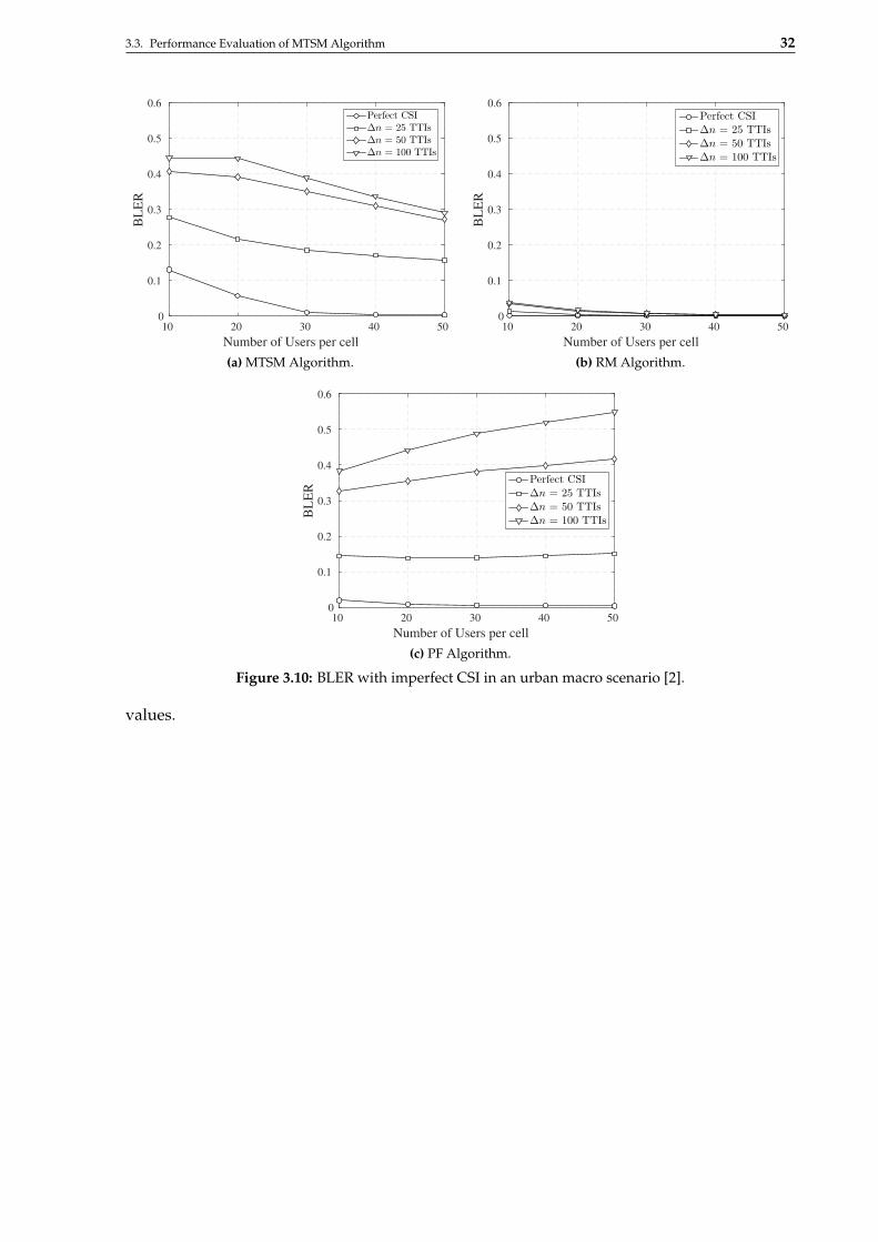
3.3. Performance Evaluation of MTSM Algorithm 32
Number of Users per cell
10 20 30 40 50
BL
ER
0
0.1
0.2
0.3
0.4
0.5
0.6Perfect CSI
∆n = 25 TTIs
∆n = 50 TTIs
∆n = 100 TTIs
(a) MTSM Algorithm.
Number of Users per cell
10 20 30 40 50
BL
ER
0
0.1
0.2
0.3
0.4
0.5
0.6
Perfect CSI
∆n = 25 TTIs
∆n = 50 TTIs
∆n = 100 TTIs
(b) RM Algorithm.
Number of Users per cell
10 20 30 40 50
BL
ER
0
0.1
0.2
0.3
0.4
0.5
0.6
Perfect CSI
∆n = 25 TTIs
∆n = 50 TTIs
∆n = 100 TTIs
(c) PF Algorithm.
Figure 3.10: BLER with imperfect CSI in an urban macro scenario [2].
values.

3.4. Performance Evaluation of MDSM Algorithm 33
3.4 Performance Evaluation of MDSM Algorithm
This section evaluates the MDSM algorithm with different configurations according to
Table 3.2, which shows the main parameters of the simulated LTE-like system network.
Table 3.2: Simulation Parameters
Parameter ValueMaximum BS transmit power 20 WBS antenna radiation pattern Three-sectoredCell radius 1 kmUE speed 3 km/hCarrier frequency 2 GHzSystem bandwidth 5 MHzSub-carrier bandwidth 15 kHzNumber of RBs 6Path loss - macro cell scenario [3] PL = 15.3 + 37.6 · log10(d)
a
Path loss - urban macro scenario [2] PL = 34.5 + 35 · log10(d)a
Channel coherence time 90 msAntenna gainb[44] Gh(θh) + Gv(θv)Downtilt angle 8 degreesLog-normal shadowing st. dev. 8 dBSmall-scale fading [43] 3GPP Typical UrbanAWGN power per sub-carrier -123.24 dBmNoise figure 9 dBLink adaptation Link level curves from [39]SNR threshold of MCS 1 [39] -6.9 dBTransmission Time Interval 1 msRT traffic model VoIPHOL packet delay requirement 40 msVoIP packet size 320 bitsMulti-antenna configuration SISOSimulation time span 30 sNumber of simulation runs 10Confidence Interval 95%a d is the distance to the BS in km.b θh and θv represent the horizontal and vertical angles related to
the BS, respectively.
3.4.1 Perfect CSI
The MDSM algorithm is initially analyzed considering the effect of the scale parameter λ in
symmetric marginal utilities. The shape parameter fixed at θ → 0. The effect of the variation of
the scale parameter is shown in Figure 3.4. We consider three different curves: wide (λ = 30 dB),
DSM (original, λ = −10 dB) and narrow(λ = −20 dB).
Figures 3.11(a) and 3.11(b) indicate the percentage of satisified users. The wide MDSM
configuration tends to allocate resources giving more importance to the channel conditions,
consequently it is less sensitive to the system load variation, since it always selects users
with the highest instantaneous data rate. As the load increases, higher gains are observed in
comparison to the other configurations. The wide configuration achieves an improvement of
20% compared with the symmetric curve (DSM) for higher loads in the macro cell scenario. It
achieves an improvement of 50% compared with the symmetric curve (DSM) for higher loads
in the urban macro scenario.

3.4. Performance Evaluation of MDSM Algorithm 34
Number of Users per cell
80 100 120 140 160 180 200
Sat
isfa
ctio
n I
ndex
0
20
40
60
80
100
Wide, λ = 30dB
DSM, λ = −10dB
Narrow, λ = −20dB
(a) User Satisfaction - macro cell scenario [3].
Number of Users per cell
80 100 120 140 160 180 200
Sat
isfa
ctio
n I
nd
ex
0
20
40
60
80
100Wide, λ = 30dB
DSM, λ = −10dB
Narrow, λ = −20dB
(b) User Satisfaction - urban macro scenario [2].
Number of Users per cell
80 100 120 140 160 180 200
Mea
n T
hro
ughput
per
Cel
l [M
bps]
0.6
0.8
1
1.2
1.4
1.6
Wide, λ = 30dB
DSM, λ = −10dB
Narrow, λ = −20dB
(c) Total cell throughput - macro cell scenario [3].
Number of Users per cell
80 100 120 140 160 180 200
Mea
n T
hro
ughput
per
Cel
l [M
bps]
0.6
0.8
1
1.2
1.4
1.6Wide, λ = 30dB
DSM, λ = −10dB
Narrow, λ = −20dB
(d) Total cell throughput - urban macro scenario [2].
Number of Users per cell
80 100 120 140 160 180 200
Fai
rnes
s In
dex
88
90
92
94
96
98
100
Wide, λ = 30dB
DSM, λ = −10dB
Narrow, λ = −20dB
(e) Mean cell fairness index - macro cell scenario [3].
Number of Users per cell
80 100 120 140 160 180 200
Fai
rnes
s In
dex
88
90
92
94
96
98
100
Wide, λ = 30dB
DSM, λ = −10dB
Narrow, λ = −20dB
(f) Mean cell fairness index - urban macro scenario [2].
Figure 3.11: Performance metrics of the MDSM algorithm as a function of the number of RT users withdifferent values of scale parameter, λ.
The narrow configuration has the lowest satisfaction indexes because penalizes users in
extreme conditions, i.e., very good or very bad users have low priority. With this, users with
better channel conditions, despite having the lowest HOL delays, are discarded since their
marginal utility tends to zero. In contrast, the wide configuration is able to distribute resources
among users with better conditions, achieving gains comparable to that observed in DSM. The

3.4. Performance Evaluation of MDSM Algorithm 35
change of channel conditions from macro cell to urban macro impacts directly the satisfaction
levels achieved by the algorithms, with a significant decrement of DSM, which decays from
70% to 10% with higher loads. The wide configuration of MDSM offers a greater resistance to
more critical channel conditions, since it distributes resources to users which are to a greater
delay in relation to the delay requirement.
The system capacity in terms of total throughput as a function of the system load is depicted
in Figure 3.11(c) and 3.11(d). The total cell throughput provided by the MDSM increases as the
system load raise for all considered configurations. The same behavior is observed with DSM.
The mean fairness index behavior as a function of the system load is depicted by
Figures 3.11(e) and 3.11(f) . The fairness levels in the macro cell scenario have the same order,
almost 1, for all loads considered. The worsening channel conditions of the urban macro
scenario result in a deterioration of fair indices, which decay to values of the order of 95%
for DSM or 90% for MDSM.
Proceeding with the evaluation, we consider the effect of the marginal utility’ asymmetry in
the MDSM algorithm. Thus, we evaluate the scheduling algorithm for RT services, extending
the study of [26], that considered a symmetric bell-shaped curve.
Therefore, we evaluate the effect of the change of the shape parameter θ of the marginal
utility function given by (3.11). Once packets with HOL packet delay higher than the
delay requirement are discarded at the transmitter, we consider negative values of the shape
parameter, θ < 0 because we are interested in curves skewed to the left side, benefiting users
with delay equal or below the requirement. The magnitude of the scale parameter θ, also
determines the behavior of the function when near the QoS requirement: higher values of the
shape parameter, in this study θ = −1, result in curves with sharper edges; lower values, here
considered θ = −0.5, imply smoother peaks. Therefore, we consider three different curves:
bell-shaped (θ → 0), left skewed with soft edge (θ = −0.5), and left skewed with sharp edge
(θ = −1.0). The simulated curves are shown in Figures 3.5(a) and 3.5(b).
The behavior of the satisfaction index of the system as a function of RT users is shown at
Figures 3.12(a) and 3.12(b). The results indicate that the left skewed configurations are able
to provide gains in the satisfactions levels in comparison with the original symmetric curve,
hence they improve the conditions of transmission of users with low HOL delay.
The left skewed with soft edge curve gives priority to a portion of users with HOL delay
higher than the requirement, while left skewed curve with sharp edge, gives zero priority to
users with HOL delay higher than the requirement. This means that the soft edge configuration
gives priority to users which will have delay higher than the requirement. Consequently,
this configuration distributes resources to users that will be unsuccessful. This is a clear
disadvantage of that configuration that results in satisfaction levels lower than those achieved
by the sharp edge configuration. In spite of this disadvantage, the left skewed soft edge MDSM
achieves gains of 15% in the satisfaction levels in comparison with DSM for a load of 200 users.
In the considered scenario, the left skewed sharp edge is the most efficient configuration to
maximize users’ satisfaction, obtaining an improvement of 20% compared with the symmetric
curve (DSM) for higher loads (200 users). Figure 3.12(b) show us that the DSM algorithm
3.4. Performance Evaluation of MDSM Algorithm 36
Number of Users per cell
80 100 120 140 160 180 200
Sat
isfa
ctio
n I
ndex
0
20
40
60
80
100
DSM, θ → 0
Left Skewed - Soft Edge, θ = −0.50
Left Skewed - Sharp Edge,θ = −1.00
(a) User Satisfaction - macro cell scenario [3].
Number of Users per cell
80 100 120 140 160 180 200
Sat
isfa
ctio
n I
ndex
0
20
40
60
80
100
DSM, θ → 0
Left Skewed - Soft Edge, θ = −0.50
Left Skewed - Sharp Edge,θ = −1.00
(b) User Satisfaction - urban macro scenario [2].
Number of Users per cell
80 100 120 140 160 180 200
Mea
n T
hro
ug
hp
ut
per
Cel
l [M
bp
s]
0.6
0.8
1
1.2
1.4
1.6
DSM, θ → 0
Left Skewed - Soft Edge, θ = −0.50
Left Skewed - Sharp Edge,θ = −1.00
(c) Total cell throughput - macro cell scenario [3].
Number of Users per cell
80 100 120 140 160 180 200
Mea
n T
hro
ughput
per
Cel
l [M
bps]
0.6
0.8
1
1.2
1.4
1.6
DSM, θ → 0
Left Skewed - Soft Edge, θ = −0.50
Left Skewed - Sharp Edge,θ = −1.00
(d) Total cell throughput - urban macro scenario [2].
Number of Users per cell
80 100 120 140 160 180 200
Fai
rnes
s In
dex
94
95
96
97
98
99
100
DSM, θ → 0
Left Skewed - Soft Edge, θ = −0.50
Left Skewed - Sharp Edge,θ = −1.00
(e) Mean cell fairness index - macro cell scenario [3].
Number of Users per cell
80 100 120 140 160 180 200
Fai
rnes
s In
dex
94
95
96
97
98
99
100
DSM, θ → 0
Left Skewed - Soft Edge, θ = −0.50
Left Skewed - Sharp Edge,θ = −1.00
(f) Mean cell fairness index - urban macro scenario [2].
Figure 3.12: Performance metrics of the MDSM algorithm as a function of the number of RT users withdifferent values of shape parameter, θ.
is more impacted by the worsening of channel conditions, while the asymmetric curves of
the MDSM configurations are able to provide a distribution of resources that improve user
satisfaction.
The system capacity in terms of total throughput is shown at Figures 3.12(c) and 3.12(d).
The proposed MDSM configurations achieved total cell throughput of the same order of

3.4. Performance Evaluation of MDSM Algorithm 37
DSM, the average data rate improvement becomes more noticeable only at higher loads. It
is also observed that the total cell throughput provided by the MDSM configurations raise
as the number of users become higher. Therefore, the proposed RRA exploit successfully the
multi-user diversity.
The mean fairness index as a function of the number of RT users is indicated in
Figures 3.12(e) and 3.12(f). The fairness levels obtained have the same order, almost 1 in
the macro cell scenario and a little bit smaller in the urban macro scenario. Therefore, the
symmetric and the left skewed marginal utility functions provide a balanced distribution of
resources.
From the discussion of the performance metrics achieved by the different shifted log-logistic
marginal utilities, we conclude that the wide configuration achieved the best results of user
satisfaction and resource efficiency. Therefore, in order to evaluate this MDSM configuration
we compare it with classical RRA algorithms found in the literature, i.e., Modified Largest
Weighted Delay First (MLWDF), Urgency and Efficiency-based Packet Scheduling (UEPS) and
DSM.
In the macro cell scenario, there is a tie between satisfaction levels achieved by MLWDF,
UEPS and MDSM algorithms, Figure 3.13(a). However, when the urban macro scenario is
considered, the MDSM achieves the highest levels of satisfaction compared with all other
algorithms, which demonstrates the advantage of using a wide marginal utility function when
satisfaction maximization is desired, as can be seen in Figure 3.13(b).
The MDSM algorithm provides good capacity results, achieving throughput of the same
order of MLWDF and UEPS, with an almost uniform behavior for different traffic loads, as can
be seen in Figures 3.13(c) and 3.13(d).
According to Figure 3.13(e), all the considered algorithms are in equal manner fair in
the macro cell scenario. The difficulties encountered in distributing resources so that users
meet the minimum requirements due to more challenging channel conditions of urban macro
scenario, implies a uneven allocation and decreases the Jains’ fairness index, as can be seen in
Figure 3.13(f)
3.4.2 Imperfect CSI
This section analyses the impacts of CSI imperfections on the performance of the DSM
algorithm. As well as done in Section 3.3.2, the CSI imperfection is modeled as a delay of
the channel measurements received by the eNB.
The MDSM algorithm is the less susceptible to CSI imperfections and maintains the highest
satisfaction levels, as indicated in Figure 3.14(a). The UEPS and MLWDF show a significant fall
in satisfaction indexes. The UEPS and MLWDF algorithms use the status of the current channel
as an indicator of the resource usage and directs the distribution of resources among users.
Therefore, they are strongly affected by a delayed CSI. With lower loads, the delay of 25 TTIs
reduces the satisfaction levels of UEPS and MLWDF in 50% while MDSM has its satisfaction
index only decreased by 10%. Considering higher loads, the decrement of satisfaction of UEPS
and MLWDF is even worse, going quickly to zero with 120 UE, and MDSM achieves levels near
to 70%.

3.4. Performance Evaluation of MDSM Algorithm 38
Number of Users per cell
80 100 120 140 160 180 200
Sat
isfa
ctio
n I
ndex
0
20
40
60
80
100
MLWDF
UEPS
DSM
MDSM
(a) User Satisfaction - macro cell scenario [3].
Number of Users per cell
80 100 120 140 160 180 200
Sat
isfa
ctio
n I
nd
ex
0
20
40
60
80
100
MLWDF
UEPS
DSM
MDSM
(b) User Satisfaction - urban macro scenario [2].
Number of Users per cell
80 100 120 140 160 180 200
Mea
n T
hro
ughput
per
Cel
l [M
bps]
0.6
0.8
1
1.2
1.4
1.6
MLWDF
UEPS
DSM
MDSM
(c) Total cell throughput - macro cell scenario [3].
Number of Users per cell
80 100 120 140 160 180 200
Mea
n T
hro
ug
hp
ut
per
Cel
l [M
bp
s]
0.6
0.8
1
1.2
1.4
1.6
MLWDF
UEPS
DSM
MDSM
(d) Total cell throughput – urban macro scenario [2].
Number of Users per cell
80 100 120 140 160 180 200
Fai
rnes
s In
dex
88
90
92
94
96
98
100
MLWDF
UEPS
DSM
MDSM
(e) Mean cell fairness index - macro cell scenario [3].
Number of Users per cell
80 100 120 140 160 180 200
Fai
rnes
s In
dex
88
90
92
94
96
98
100
MLWDF
UEPS
DSM
MDSM
(f) Mean cell fairness index - urban macro scenario [2].
Figure 3.13: Performance metrics of the MDSM algorithm compared with the algorithms MLWDF,UEPS and DSM.
The considered model of RT services implies low data traffic demand. Therefore, the
imperfection of CSI has low impact over the mean throughput per cell, as can be seen in Figure
3.14(b). The impact of imperfect CSI on the algorithms can be neglected for small measurement
delays, such as ∆n = 25 TTIs or ∆n = 50 TTIs . However, if the delay is greater than half the
channel coherence time, the CSI and the real channel become almost uncorrelated. This fact

3.4. Performance Evaluation of MDSM Algorithm 39
Number of Users per cell
80 100 120 140 160 180 200
Sat
isfa
ctio
n I
ndex
0
20
40
60
80
100
Perfect CSI
∆n = 25 TTIs
∆n = 50 TTIs
∆n = 100 TTIs
MDSM
UEPS
MLWDF
(a) User Satisfaction index.
Number of Users per cell
80 100 120 140 160 180 200
Mea
n T
hro
ugh
pu
t p
er C
ell
[Mb
ps]
0
0.2
0.4
0.6
0.8
1
1.2
1.4
1.6Perfect CSI
∆n = 25 TTIs
∆n = 50 TTIs
∆n = 100 TTIs
MDSM
UEPS
MLWDF
(b) Total Cell Throughput.
Figure 3.14: Performance metrics of the MDSM algorithm compared with classical algorithmsconsidering imperfect CSI in an urban macro scenario [2].
Number of Users per cell
80 100 120 140 160 180 200
BL
ER
0
0.1
0.2
0.3
0.4
0.5
0.6
0.7
0.8
Perfect CSI
∆n = 25 TTIs
∆n = 50 TTIs
∆n = 100 TTIs
(a) MDSM Algorithm.
Number of Users per cell
80 100 120 140 160 180 200
BL
ER
0
0.1
0.2
0.3
0.4
0.5
0.6
0.7
0.8
Perfect CSI
∆n = 25 TTIs
∆n = 50 TTIs
∆n = 100 TTIs
(b) UEPS Algorithm.
Number of Users per cell
80 100 120 140 160 180 200
BL
ER
0
0.1
0.2
0.3
0.4
0.5
0.6
0.7
0.8
Perfect CSI
∆n = 25 TTIs
∆n = 50 TTIs
∆n = 100 TTIs
(c) MLWDF Algorithm.
Figure 3.15: BLER with imperfect CSI in an urban macro scenario [2].
decreases the eNB throughput moderately by increasing the BLER to unacceptable values.

3.5. Partial Conclusions 40
3.5 Partial Conclusions
The determination of the function to be used in a utility-based scheduling framework
depends on the goal the one wants to achieve. This study demonstrated by means of
system-level simulations that the shifted log-logistic function is effective towards the objective
of user satisfaction maximization, achieving gains in comparison with classical algorithms.
The MTSM algorithm obtains significant gains when employing asymmetric marginal
utility functions, enabling a stable strategy maximize user satisfaction and keep the spectral
efficiency at satisfactory levels for the entire load range considered. The best performance
results, achieved with a left skewed and soft edge curve, indicate an increment of 30% of the
users’ satisfaction levels for higher loads.
The MDSM algorithm also attained gains with the use of asymmetric marginal utility
functions. Differently from previously noticed with MTSM, variations in the aperture of the
function, i.e., a more flattened curve also provided gains in the users’ satisfaction. The best
performance results, achieved with a wider curve, indicate an increment of 20% of the users’
satisfaction levels for higher loads.
Chapter 4Scheduling Framework for Adaptive
Satisfaction Control
In this chapter, the problem of controlling the user satisfaction is further investigated
considering the dynamic and adaptive variation of the parameters of the shifted log-logistic
function. Section 4.1 provides a general description of the shifted log-logistic utility
function. Sections 4.2 and 4.3 present two adaptive algorithms, describing the extension
of the utility-based framework described previously and Section 4.4 evaluate the proposed
algorithms. Finally, Section 4.5 provides a partial conclusion based on the system-level
simulation results.
4.1 Shifted Log-Logistic Utility Function
In this study, we develop a general scheduling framework that is able to control the degree
to which a network satisfies service requirements of users’ applications in terms of throughput.
In other words, this research investigates novel ways to control the satisfaction level of users
of Non-Real Time (NRT) services. In this context, we evaluate different methods to solve this
problem extending the framework based on utility theory proposed in [26] and described in
details in Chapter 3.
The present study extends the investigation of utility-based scheduling algorithms,
analyzing adaptive policies using the shifted log logistic utility function. This function is
represented by
US-Log(T?j [n]) =
1
1 +
(1 +
θ(T?j [n]− T?req
j )
λ
)−1/θ, (4.1)
where T?j is the throughput of user j and T?req
j is the required throughput; θ is a real parameter
which determines the shape of the function and λ is a real parameter that sets the scale of the
function.
Without loss of generality, it is considered Tj normalized by the Quality of Service (QoS)
requirement, i.e., Tj = T?j /T?req
j and Treqj = T?req
j /T?reqj = 1 and US-Log(T?
j [n]) is simply
replaced by US-Log(Tj[n]) hereafter.
4.2. Adaptive Throughput-Based Efficiency-Satisfaction Trade-Off Algorithm 42
The shifted log-logistic utility function is limited by Tj[n] intervals, according to the values
of θ, λ and Treqj . Given θ > 0, US-Log = 1 if Tj[n] < Treq
j − λ
θ. Considering θ < 0, US-Log = 1 if
Tj[n] > Treqj − λ
θ.
The function indicated by (4.1) is continuous, differentiable over the range Tj[n], and limited
between 0 and 1, i.e. 0 ≤ US-Log ≤ 1.
The utility-based weight performs an important function in the scheduling algorithm, once
the priority of a given user to get a resource is directly proportional to this weight. The shifted
log-logistic marginal utility is given by
wS-Logj =
1λ
(1 +
θ(Tj[n]− Treqj )
λ
)−1−1/θ
1 +
(1 +
θ(Tj[n]− Treqj )
λ
)−1/θ2 , (4.2)
As mentioned previously, the marginal utility function has two parameters, θ and λ, that
clearly impact its behavior, allowing different scheduling strategies to be configured by an
adequate parameter setting. The shape parameter, θ, impacts the symmetry of the marginal
utility curve, while the scale parameter λ, influences the peakedness of symmetric curves.
This study explores the dynamic variation of the two parameters of the shifted log-logistic
function in the scheduling, showing that it is possible to control the satisfaction levels by
suitable arrangements of these parameters. The proposed algorithms that are obtained by
the variation of each of these parameters separately are called Adaptive Throughput-based
Efficiency-Satisfaction Trade-Off (ATES) and Adaptive Satisfaction Control (ASC) and are
described in the following sections. Figure 4.1 depicts the extension on the scheduling
procedure described by [26].
The considered algorithms exploit in a widely way the multi-user diversity, since the shifted
log-logistic utility function covers a larger range of variations for the considered QoS metric.
System level simulation results demonstrate that it is possible to mimic different scheduling
algorithms by modifying the framework parameters while maintaining user satisfaction at
defined levels for different system loads considering NRT services.
4.2 Adaptive Throughput-Based Efficiency-Satisfaction Trade-Off Algorithm
The ATES algorithm aims to deal with the trade-off between resource efficiency and
satisfaction planned by the network operator in a scenario with NRT services. This is done
by means of a dynamic control of the scale parameter of the marginal utility function.
The ATES technique dynamically adapts the scale parameter of the shifted log-logistic
rule framework aiming to achieve a desired throughput-based satisfaction distribution among
users. This strategy provides a strict control of the network QoS and has a good prediction in
terms of system capacity.
To keep satisfaction around a target value, the λ parameter is calculated using a control
4.2. Adaptive Throughput-Based Efficiency-Satisfaction Trade-Off Algorithm 43
Figure 4.1: Adaptive scheduling algorithms flow-chart.
loop of the form
λ[n] = λ[n− 1]− η(ΥFilt − ΥTarget), (4.3)
where η is a step size that determines the speed of adaptation of λ; ΥFilt is a filtered satisfaction
percentage and ΥTarget is the target satisfaction. To ensure the convergence, the λ parameter
is limited by an interval given by [λmin, λmax]. A block diagram representation of the scale
parameter control loop is depicted in Figure 4.2.
Modifications of the scale parameter vary the format of the utility function as indicated in
Figure 4.3(a). The increase of λ, indicated by the arrows, makes the step less abrupt. This
Figure 4.2: Block diagram representation of (4.3).

4.3. Adaptive Satisfaction Control Algorithm 44
behavior means that the user becomes satisfied more slowly if the user throughput approaches
the requirement. The marginal utility function, represented in Figure 4.3(b), has its peakedness
reduced by the increase of λ, as indicated by the arrow in the figure. Lower values of the
scale parameter imply a scheduling process that give higher priority to users experiencing
throughput levels close to the requirement.
Normalized QoS Metric
0 0.5 1 1.5 2
Uti
lity
0
0.2
0.4
0.6
0.8
1
(a) Utility function
Normalized QoS Metric
0 0.5 1 1.5 2
Mar
gin
al U
tili
ty
0
0.5
1
1.5
2
2.5
3
(b) Marginal utility function
Figure 4.3: Behavior of US-Log and wS-Log with a fixed shape parameter (θ → 0) and different values ofthe scale parameter λ.
4.3 Adaptive Satisfaction Control Algorithm
The ASC algorithm controls the shape parameter of the shifted log-logistic function. The
adaptive equation is given by
θ[n] = θ[n− 1]− ε(ΥFilt − ΥTarget), (4.4)
where ε is a constant that establishes the speed of adaptation of θ; ΥFilt is a filtered satisfaction
percentage and ΥTarget is the target satisfaction percentage. The θ parameter is limited to
the range [θmin, θmax] to prevent dispersion of the algorithm. The scale parameter is fixed
at λ = 0.1088, the standard value previously established on Chapter 3. A block diagram
representation of the shape parameter control loop is depicted in Figure 4.4.
The shape parameter allows a different control of the format of the marginal utility function
in comparison with the changes determined by (4.3). The ASC algorithm considers the absolute
value and the sign of the shape parameter. As a consequence, it makes possible prioritizing
users through different manners and it improves the conditions of the algorithm to control the
satisfaction of the users in the system.
The signal of the θ parameter determines the direction of the marginal utility curve. Positive
values of θ imply right tailed curves while negative values determine left tailed curves.
Figure 4.5(a) indicates the changes in the format of the utility function with the variation of
the absolute value of θ, considering only negative values of the shape parameter, θ < 0.
In this study, only negative values of θ are considered because the evaluation of Modified
Throughput-based Satisfaction Maximization (MTSM) demonstrated that this configuration
provides the maximum satisfaction level for a large amount of users in comparison with
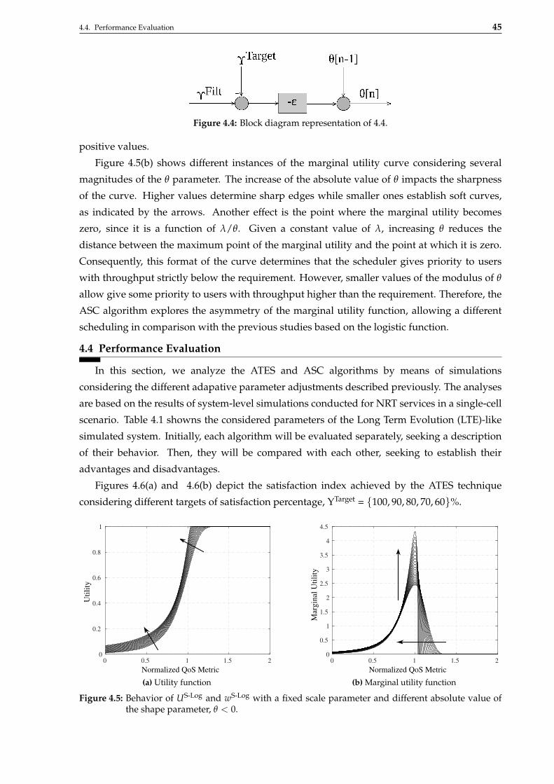
4.4. Performance Evaluation 45
Figure 4.4: Block diagram representation of 4.4.
positive values.
Figure 4.5(b) shows different instances of the marginal utility curve considering several
magnitudes of the θ parameter. The increase of the absolute value of θ impacts the sharpness
of the curve. Higher values determine sharp edges while smaller ones establish soft curves,
as indicated by the arrows. Another effect is the point where the marginal utility becomes
zero, since it is a function of λ/θ. Given a constant value of λ, increasing θ reduces the
distance between the maximum point of the marginal utility and the point at which it is zero.
Consequently, this format of the curve determines that the scheduler gives priority to users
with throughput strictly below the requirement. However, smaller values of the modulus of θ
allow give some priority to users with throughput higher than the requirement. Therefore, the
ASC algorithm explores the asymmetry of the marginal utility function, allowing a different
scheduling in comparison with the previous studies based on the logistic function.
4.4 Performance Evaluation
In this section, we analyze the ATES and ASC algorithms by means of simulations
considering the different adapative parameter adjustments described previously. The analyses
are based on the results of system-level simulations conducted for NRT services in a single-cell
scenario. Table 4.1 showns the considered parameters of the Long Term Evolution (LTE)-like
simulated system. Initially, each algorithm will be evaluated separately, seeking a description
of their behavior. Then, they will be compared with each other, seeking to establish their
advantages and disadvantages.
Figures 4.6(a) and 4.6(b) depict the satisfaction index achieved by the ATES technique
considering different targets of satisfaction percentage, ΥTarget = {100, 90, 80, 70, 60}%.
Normalized QoS Metric
0 0.5 1 1.5 2
Uti
lity
0
0.2
0.4
0.6
0.8
1
(a) Utility function
Normalized QoS Metric
0 0.5 1 1.5 2
Mar
gin
al U
tili
ty
0
0.5
1
1.5
2
2.5
3
3.5
4
4.5
(b) Marginal utility function
Figure 4.5: Behavior of US-Log and wS-Log with a fixed scale parameter and different absolute value ofthe shape parameter, θ < 0.

4.4. Performance Evaluation 46
Table 4.1: Simulation Parameters of ASC and ATES Evaluation
Parameter ValueMaximum BS transmit power 20 WBS antenna radiation pattern Three-sectoredCell radius 1 kmUE speed 3 km/hCarrier frequency 2 GHzSystem bandwidth 5 MHzSub-carrier bandwidth 15 kHzNumber of Resource Blocks (RBs) 25 NRTPath loss - macro cell scenario [3] PL = 15.3 + 37.6 · log10(d)
a
Path loss - urban macro scenario [2] PL = 34.5 + 35 · log10(d)a
Channel coherence time 90 msAntenna gainb[44] Gh(θh) + Gv(θv)Downtilt angle 8 degreesLog-normal shadowing st. dev. 8 dBSmall-scale fading [43] 3GPP Typical UrbanAWGN power per sub-carrier -123.24 dBmNoise figure 9 dBLink adaptation Link level curves from [39]SNR threshold of MCS 1 [39] -6.9 dBTransmission Time Interval 1 msNRT traffic model Full bufferUser throughput requirement VariableMulti-antenna configuration SISOSatisfaction target (ΥTarget) VariableMinimum scale parameter (λmin) -50 dBMaximum scale parameter ( λmax) -10 dBATES step size (η) 0.10Minimum shape parameter (θmin) -5.0Maximum shape parameter ( θmax) -0.5ASC step size (ε) 0.10Simulation time span 10 sNumber of simulation runs 75Confidence Interval 95%a d is the distance to the BS in km.b θh and θv represent the horizontal and vertical angles related to
the Base Station (BS), respectively.
The ATES technique is capable of reaching levels of satisfaction around the planned value
in the macro cell scenario, as can be seen in Figure 4.6(a). If worst channel conditions are
considered like the urban macro scenario, as depicted in Figure 4.6(b) , only the smaller targets
are achieved for a wide range of users.
Therefore, ATES technique keeps the satisfaction percentage near the requirement in the
macro cell scenario, but in all cases the target is not met exactly. These results show that
the dynamic variation of peakedness of symmetric curves cannot explore successfully the
resources, since it gives the same priority to users with QoS near the throughput requirement
and does not consider a large set of users with worse conditions. This explains the decrease
of the accuracy observed for higher loads (above 30 users), when the satisfaction levels decay
almost 15%.
Figures 4.6(c) and 4.6(d) show the mean throughput per cell as a function of the number of
users in the system. The ATES algorithm provides different throughput values depending
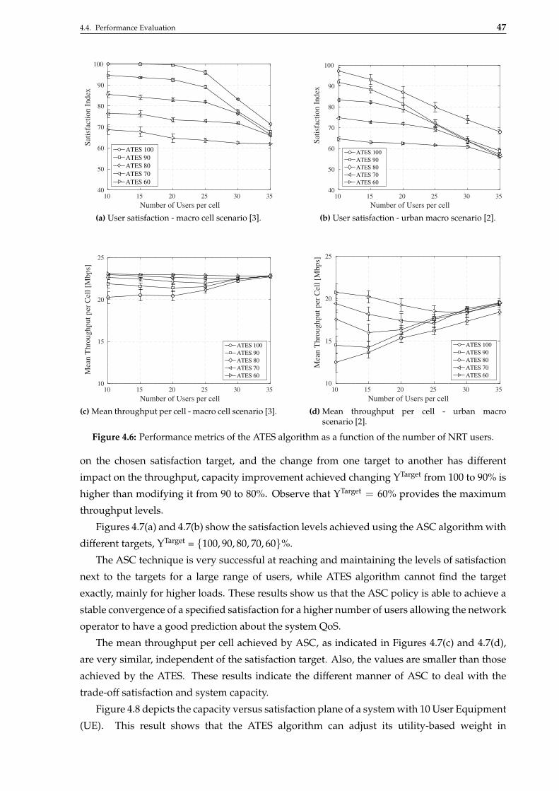
4.4. Performance Evaluation 47
Number of Users per cell
10 15 20 25 30 35
Sat
isfa
ctio
n I
ndex
40
50
60
70
80
90
100
ATES 100
ATES 90
ATES 80
ATES 70
ATES 60
(a) User satisfaction - macro cell scenario [3].Number of Users per cell
10 15 20 25 30 35
Sat
isfa
ctio
n I
ndex
40
50
60
70
80
90
100
ATES 100
ATES 90
ATES 80
ATES 70
ATES 60
(b) User satisfaction - urban macro scenario [2].
Number of Users per cell
10 15 20 25 30 35
Mea
n T
hro
ughput
per
Cel
l [M
bps]
10
15
20
25
ATES 100
ATES 90
ATES 80
ATES 70
ATES 60
(c) Mean throughput per cell - macro cell scenario [3].
Number of Users per cell
10 15 20 25 30 35
Mea
n T
hro
ughput
per
Cel
l [M
bps]
10
15
20
25
ATES 100
ATES 90
ATES 80
ATES 70
ATES 60
(d) Mean throughput per cell - urban macroscenario [2].
Figure 4.6: Performance metrics of the ATES algorithm as a function of the number of NRT users.
on the chosen satisfaction target, and the change from one target to another has different
impact on the throughput, capacity improvement achieved changing ΥTarget from 100 to 90% is
higher than modifying it from 90 to 80%. Observe that ΥTarget = 60% provides the maximum
throughput levels.
Figures 4.7(a) and 4.7(b) show the satisfaction levels achieved using the ASC algorithm with
different targets, ΥTarget = {100, 90, 80, 70, 60}%.
The ASC technique is very successful at reaching and maintaining the levels of satisfaction
next to the targets for a large range of users, while ATES algorithm cannot find the target
exactly, mainly for higher loads. These results show us that the ASC policy is able to achieve a
stable convergence of a specified satisfaction for a higher number of users allowing the network
operator to have a good prediction about the system QoS.
The mean throughput per cell achieved by ASC, as indicated in Figures 4.7(c) and 4.7(d),
are very similar, independent of the satisfaction target. Also, the values are smaller than those
achieved by the ATES. These results indicate the different manner of ASC to deal with the
trade-off satisfaction and system capacity.
Figure 4.8 depicts the capacity versus satisfaction plane of a system with 10 User Equipment
(UE). This result shows that the ATES algorithm can adjust its utility-based weight in

4.4. Performance Evaluation 48
Number of Users per cell
10 15 20 25 30 35
Sat
isfa
ctio
n I
ndex
40
50
60
70
80
90
100
ASC 100
ASC 90
ASC 80
ASC 70
ASC 60
(a) User satisfaction - macro cell scenario [3].
Number of Users per cell
10 15 20 25 30 35
Sat
isfa
ctio
n I
ndex
40
50
60
70
80
90
100
ASC 100
ASC 90
ASC 80
ASC 70
ASC 60
(b) User satisfaction - urban macro scenario [2].
Number of Users per cell
10 15 20 25 30 35
Mea
n T
hro
ug
hp
ut
per
Cel
l [M
bp
s]
8
10
12
14
16
18
20
22
ASC 100
ASC 90
ASC 80
ASC 70
ASC 60
(c) Mean throughput per cell - macro cell scenario [3].Number of Users per cell
10 15 20 25 30 35
Mea
n T
hro
ughput
per
Cel
l [M
bps]
8
10
12
14
16
18
20
22
ASC 100
ASC 90
ASC 80
ASC 70
ASC 60
(d) Mean throughput per cell - urban macroscenario [2].
Figure 4.7: Performance metrics of the ASC algorithm as a function of the number of NRT users.
Satisfaction Index
50 55 60 65 70 75
Mea
n T
hro
ug
hp
ut
per
Cel
l [M
bp
s]
20
20.5
21
21.5
22
22.5
23
23.5
24ATES
ASC
Figure 4.8: Capacity vs Satisfaction plane considering a system load of 10 users - macro cell scenario [3].
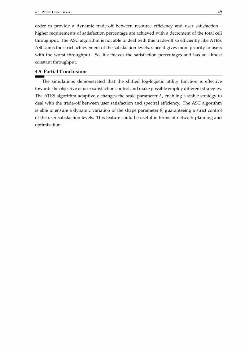
4.5. Partial Conclusions 49
order to provide a dynamic trade-off between resource efficiency and user satisfaction -
higher requirements of satisfaction percentage are achieved with a decrement of the total cell
throughput. The ASC algorithm is not able to deal with this trade-off so efficiently like ATES.
ASC aims the strict achievement of the satisfaction levels, since it gives more priority to users
with the worst throughput. So, it achieves the satisfaction percentages and has an almost
constant throughput.
4.5 Partial Conclusions
The simulations demonstrated that the shifted log-logistic utility function is effective
towards the objective of user satisfaction control and make possible employ different strategies.
The ATES algorithm adaptively changes the scale parameter λ, enabling a stable strategy to
deal with the trade-off between user satisfaction and spectral efficiency. The ASC algorithm
is able to ensure a dynamic variation of the shape parameter θ, guaranteeing a strict control
of the user satisfaction levels. This feature could be useful in terms of network planning and
optimization.
Chapter 5Conclusions
This thesis deals with scheduling algorithms aiming at the maximization and adaptive
control of the satisfaction index in the downlink of an Orthogonal Frequency Division
Multiple Access (OFDMA) network, considering different types of traffic models. In order
to solve the problem of maximizing the satisfaction with affordable complexity, a cross layer
optimization approach uses the utility theory to formulate the problem as a weighted sum
rate maximization. Chapter 3 provides some insight on the nature of the mentioned problem,
presenting the mathematical formulation of the utility-based scheduling framework.
The determination of the function to be used in the utility-based scheduling framework
depends on the desired objectives. This thesis studies two utility functions. Initially, we
consider the logistic function, to standardize the framework proposed in [26]. Next, we analyze
the shifted log-logistic function, a generalization of the logistic function. The shifted log-logistic
function has more parameters, which allows novel scheduling strategies and impacts the
distribution of resources among users. Therefore, the new framework considers different
strategies of Quality of Service (QoS)-based priorization and channel opportunism, for an equal
power allocation among frequency resources.
Chapter 3 considers the problem of improving the percentage of satisfied users. Novel
scheduling algorithms that employ different symmetric and asymmetric marginal utility
functions are evaluated: Modified Throughput-based Satisfaction Maximization (MTSM) and
Modified Delay-based Satisfaction Maximization (MDSM). The various function forms are
obtained from the modification of the shape and scale parameters of the shifted log-logistic
function. On one hand, MTSM aims to improve satisfaction index among Non-Real Time (NRT)
users in a cellular network. On the other hand, MDSM aims to maximize satisfaction among
Real Time (RT) users.
The MTSM algorithm obtains significant gains with the use asymmetric marginal utility
functions based on throughput with maximum point in the users’ throughput requirement,
enabling a stable strategy to maximize user satisfaction and keep the spectral efficiency at
satisfactory levels for the entire load range considered. The best performance results, achieved
with a left skewed and soft edge curve achieved a significant improvement of the users
satisfaction levels in comparison with Throughput-based Satisfaction Maximization (TSM) and

51
the classical algorithms Proportional Fair (PF) and Rate Maximization (RM).
The MDSM algorithm also attained gains with the employment of asymmetric marginal
utility functions. Differently from MTSM, uses a marginal utility function based on
Head Of Line (HOL) packet delay with maximum point in the users’ HOL packet delay
requirement, which is usually equal to the RT delay budget of the system. MDSM achieved
gains with symmetric and asymmetric curves. In contrast with MTSM, variations in the
aperture of the marginal utility curve, i.e., a more flattened curve also provided gains
in the users’ satisfaction, outperforming Delay-based Satisfaction Maximization (DSM) and
classical algorithms Modified Largest Weighted Delay First (MLWDF) and Urgency and
Efficiency-based Packet Scheduling (UEPS).
In realistic scenarios, imperfect Channel State Information (CSI) at the transmitter can
induce the scheduling of a user whose real channel state cannot support a required data rate,
harming the system performance. Chapter 3 also evaluates the impact of the CSI imperfection
on the performance of MTSM and MDSM.
Even presenting larger sensitivity to CSI imperfections, since they schedule user
considering a QoS-based utility function it is more likely to incur an improper scheduling
decisions due to delayed CSI measurements. MTSM and MDSM achieve higher User
Equipment (UE) satisfaction percentages than the classical algorithms.
Therefore, the system level simulations indicate the accomplishment of the objective
of proposing efficient and low complexity scheduling techniques able to maximize user
satisfaction in different scenarios with NRT and RT services.
Chapter 4 investigates novel ways to control the satisfaction level of users of NRT services.
This thesis evaluates two algorithms using the shifted log-logistic utility function: Adaptive
Throughput-based Efficiency-Satisfaction Trade-Off (ATES) and Adaptive Satisfaction Control
(ASC). The ATES algorithm performs an average satisfaction control by adaptively changing
the scale parameter, using a feedback control loop that tracks the overall satisfaction of the
users and keep it around the desired target value, enabling a stable strategy to deal with the
trade-off between satisfaction and capacity. The ASC algorithm is able to ensure a dynamic
variation of the shape parameter, guaranteeing a strict control of the user satisfaction levels.
This is a strategic advantage to the network operator who is able to design and operate the
network according to a planned user satisfaction profile.
Thereby, the system level simulations indicate the accomplishment of the objective of
development of adaptive scheduling techniques able to control user satisfaction indexes for
different system loads considering NRT services.
Some perspectives of future work include :
I evaluation of others traffic models to broaden our understanding of the applicability of
the proposed scheduling algorithms;
I shift to a multi-cellular network and develop inteference management features is a
interesting feature to evaluate the algorithms in a more realistic scenario;
I consider the provement of Quality of Experience (QoE): an increasingly number of

52
studies is focusing on delivering high-quality service experience instead of technical
requirements indicated by QoS indicators, like throughput or HOL delay.
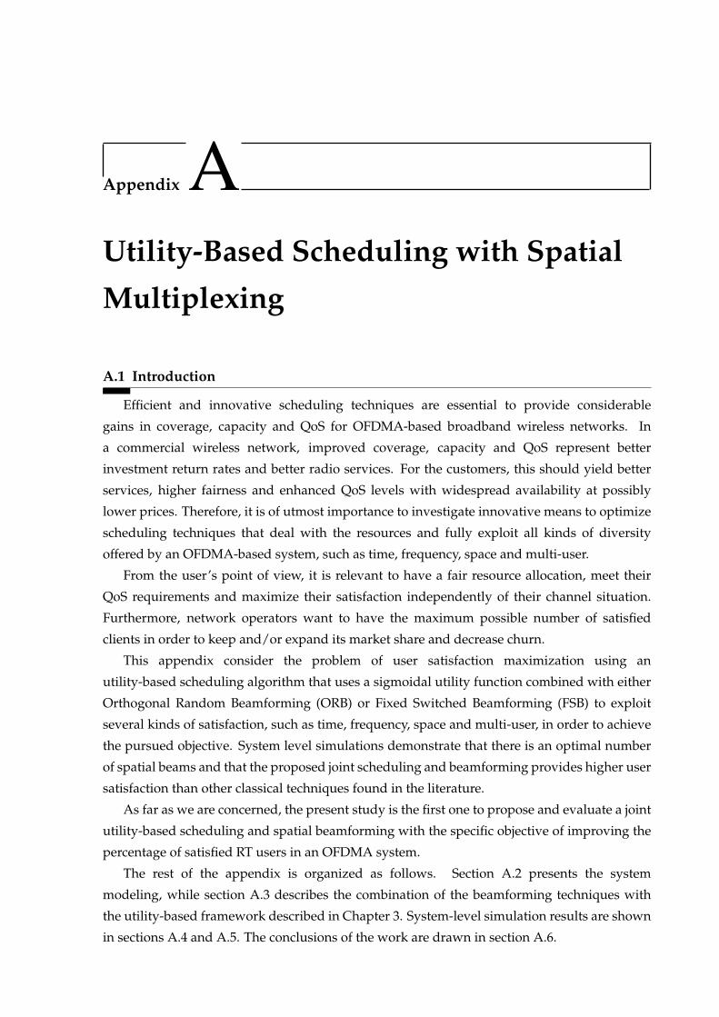
Appendix AUtility-Based Scheduling with Spatial
Multiplexing
A.1 Introduction
Efficient and innovative scheduling techniques are essential to provide considerable
gains in coverage, capacity and QoS for OFDMA-based broadband wireless networks. In
a commercial wireless network, improved coverage, capacity and QoS represent better
investment return rates and better radio services. For the customers, this should yield better
services, higher fairness and enhanced QoS levels with widespread availability at possibly
lower prices. Therefore, it is of utmost importance to investigate innovative means to optimize
scheduling techniques that deal with the resources and fully exploit all kinds of diversity
offered by an OFDMA-based system, such as time, frequency, space and multi-user.
From the user’s point of view, it is relevant to have a fair resource allocation, meet their
QoS requirements and maximize their satisfaction independently of their channel situation.
Furthermore, network operators want to have the maximum possible number of satisfied
clients in order to keep and/or expand its market share and decrease churn.
This appendix consider the problem of user satisfaction maximization using an
utility-based scheduling algorithm that uses a sigmoidal utility function combined with either
Orthogonal Random Beamforming (ORB) or Fixed Switched Beamforming (FSB) to exploit
several kinds of satisfaction, such as time, frequency, space and multi-user, in order to achieve
the pursued objective. System level simulations demonstrate that there is an optimal number
of spatial beams and that the proposed joint scheduling and beamforming provides higher user
satisfaction than other classical techniques found in the literature.
As far as we are concerned, the present study is the first one to propose and evaluate a joint
utility-based scheduling and spatial beamforming with the specific objective of improving the
percentage of satisfied RT users in an OFDMA system.
The rest of the appendix is organized as follows. Section A.2 presents the system
modeling, while section A.3 describes the combination of the beamforming techniques with
the utility-based framework described in Chapter 3. System-level simulation results are shown
in sections A.4 and A.5. The conclusions of the work are drawn in section A.6.
A.2. System Model 54
A.2 System Model
As mentioned earlier, it is considered an OFDMA system where all users form a set J with
size J, and all Resource Blocks (RBs) to be assigned to the users form a set K with size K.
It also assumed a downlink Multiple Input Single Output (MISO) channel with MT transmit
antennas at the Evolved Node B (eNB) and a single receive antenna at the terminals, and Hj,k
is an 1 × MT matrix whose elements hj,k,m consist in the channel transfer function between
the receive antenna of terminal j and the transmit antenna m of the Base Station (BS) on RB
k. The channel transfer function of the RB is aproximated by the transfer function of the mid
sub-carrier that composes the block. Furthermore, it is assumed that the channel coefficients
remain constant during the period of a Transmission Time Interval (TTI). Also, perfect channel
state information is assumed at both transmitter and receiver.
In a Multi-User (MU)-MISO scenario, the BS can steer a narrow beam b towards a direction
of interest by weighting the signal sent by each of its antennas. The complex weights wk,b
used to steer beam b on RB k are organized in a beamforming vector. From the whole set of
beamforming vectors available for transmission on an RB k, the BS can choose to transmit using
a subset Bk of active beams with size Bk, where Bk ≤ MT in order to limit intercell interference.
Using such Bk beams, the BS spatially multiplex different users on RB k.
The total BS transmit power Pt is constant and equally distributed among the RBs.
Furthermore, the power pk of each RB is equally divided between the Bk active beams.
Therefore, the power on beam b of the RB k assigned to a terminal j is denoted by pj,k,b and
given by pk/Bk.
It is not considered the intra-cell interference in the scheduling decisions. After resource
allocation, terminal j is subject to intra-cell interference from other terminals to which other
beams have been assigned on the same resource. Users’ data rates are determined using a link
adaptation curve considering the Signal to Interference-plus-Noise Ratio (SINR) values after
resource allocation [39].
A.3 Spatial Multiplexing
Figure A.1 shows examples of radiation pattern of ORB with 2 beams and FSB with 4 beams.
On one hand, ORB creates very large beams, and so a higher coverage can be obtained. This
feature is very useful for systems with a large number of users. Notice that where a given
beam presents the maximum gain, there is a null on the other beam. On the other hand, FSB
produces narrow and directed beams, which reduces the spatial interference. Notice that these
beamforming patterns must be combined with the three-sectored radiation pattern of the BS.
More details about how the beamforming vectors are generated by ORB and FSB are given in
the following.
A.3.1 Orthogonal Random Beamforming
The ORB strategy generates Bk ≤ MT orthogonal random beams on each RB k, where Bk
different users can be spatially multiplexed. Random vectors given by wk,b ∼ CN (0, 1) are
generated and the beamforming vectors wk,b in Bk are obtained by an orthonormalization of
wk,b. For Bk > 1, the weighting vectors are forced to be orthogonal to each other and to have
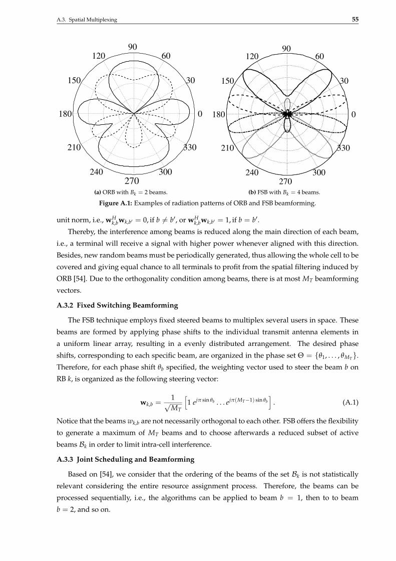
A.3. Spatial Multiplexing 55
30
210
60
240
90
270
120
300
150
330
180 0
(a) ORB with Bk = 2 beams.
60
90
120
150
180
210
240
270
300
330
0
30
(b) FSB with Bk = 4 beams.
Figure A.1: Examples of radiation patterns of ORB and FSB beamforming.
unit norm, i.e., wHk,bwk,b′ = 0, if b 6= b′, or wH
k,bwk,b′ = 1, if b = b′.
Thereby, the interference among beams is reduced along the main direction of each beam,
i.e., a terminal will receive a signal with higher power whenever aligned with this direction.
Besides, new random beams must be periodically generated, thus allowing the whole cell to be
covered and giving equal chance to all terminals to profit from the spatial filtering induced by
ORB [54]. Due to the orthogonality condition among beams, there is at most MT beamforming
vectors.
A.3.2 Fixed Switching Beamforming
The FSB technique employs fixed steered beams to multiplex several users in space. These
beams are formed by applying phase shifts to the individual transmit antenna elements in
a uniform linear array, resulting in a evenly distributed arrangement. The desired phase
shifts, corresponding to each specific beam, are organized in the phase set Θ = {θ1, . . . , θMT}.Therefore, for each phase shift θb specified, the weighting vector used to steer the beam b on
RB k, is organized as the following steering vector:
wk,b =1√MT
[1 ejπ sin θb . . . ejπ(MT−1) sin θb
]. (A.1)
Notice that the beams wk,b are not necessarily orthogonal to each other. FSB offers the flexibility
to generate a maximum of MT beams and to choose afterwards a reduced subset of active
beams Bk in order to limit intra-cell interference.
A.3.3 Joint Scheduling and Beamforming
Based on [54], we consider that the ordering of the beams of the set Bk is not statistically
relevant considering the entire resource assignment process. Therefore, the beams can be
processed sequentially, i.e., the algorithms can be applied to beam b = 1, then to to beam
b = 2, and so on.
A.4. Performance Evaluation of NRT Service Scenario 56
The scheduling is done on a TTI basis. It is controlled by a priority assignment map A ∈RJ×K×MT . This map represents the priorities of the users for all RBs and beams, where MT
upper limits Bk, ∀k. If more than one user has the same priority for the same RB and beam, a
tiebreaker process selects the user with the highest Signal to Noise Ratio (SNR).
An extension of a scheduling algorithm to cope with beamforming techniques was
proposed by [54]. Based on that, we adapted our utility-based Dynamic Resource Assignment
(DRA) algorithm. Two modifications intended to limit spatial interference were made:
I Avoidance of self-interference: whenever a beam b of RB k is allocated to user j, all the
other beams b′ 6= b on RB k are blocked to user j. This condition prevents user j from
being allocated to multiple beams of the same RB, and so user j does not interfere with
himself.
I Locking of beams/resources: whenever all Bk beams of the RB k are allocated to users, RB
k is withdrawn from the set K of available RBs. Whenever user j is allocated the beam b
of RB k, this beam is blocked to all others users j′ 6= j. However, the other beams b′ 6= b of
RB k remain free to be assigned to other users j′ 6= j. This condition avoids that multiple
users be allocated to the same beam of a given RB.
A.4 Performance Evaluation of NRT Service Scenario
In this section we firstly investigate the performance of the TSM scheduler with/without
the use of FSB beamforming. Next, the TSM+FSB technique is compared with other
classical scheduling algorithms found in the literature, such as RM [49], PF [18] and
Satisfaction-Oriented Resource Allocation for Non-Real Time Services (SORA-NRT) [23, 54].
Notice that the classical algorithms were also extended to work with FSB. Analyses are
based on the results of system-level simulations conducted for NRT services. The simulation
parameters are presented in Table A.1.
The performance of the TSM algorithm with/without FSB is evaluated considering
different numbers of active beams, in comparison with the Single Input Single Output (SISO)
scenario. A total number of MT = 8 transmit antennas is considered at the BS and the number
of active beams Bk is varied from 1 to 4. Therefore, the beamforming configurations analyzed
are denominated TSM FSB1, FSB2, FSB3 and FSB4.
Figure A.2 shows the system capacity in terms of total cell throughput as a function of the
number of NRT users (system load). Considering the SISO case, the total throughput provided
by TSM increases as the system load also increases. This means that TSM indeed exploits
multi-user diversity while tries to keep all users as satisfied as possible.
The combinations TSM FSB1 and FSB2 also preserve the ability of exploiting multi-user
diversity whereas it is benefited by two advantages brought by multiple antennas: i) the array
gain that enhances signal quality; and ii) spatial diversity due to spatially distributed beams.
Therefore, TSM and FSB are able to improve the system throughput. TSM FSB2 provides
meaningful gains (about 20% to 30%) compared to TSM SISO. The performance of TSM FSB3
and TSM FSB4 is worse than the cases with 1 and 2 active beams. The explanation for this
behavior is that the power of each RB pk has to be divided among more beams, which decreases

A.4. Performance Evaluation of NRT Service Scenario 57
Table A.1: Simulation Parameters - NRT Service Scenario
Parameter ValueNumber of cells 1Maximum BS transmit power 1 WBS antenna radiation pattern Three-sectoredCell radius 250 mUE speed 3 km/hCarrier frequency 2 GHzSystem bandwidth 5 MHzSub-carrier bandwidth 15 kHzNumber of RBs 25Path lossa L = 128.1 + 37.6 log10 dLog-normal shadowing st. dev. 8 dBSmall-scale fading [43] 3GPP Typical UrbanAWGN power per sub-carrier -123.24 dBmNoise figure 9 dBLink adaptation Link level curves from [39]Transmission Time Interval 1 msNRT traffic model Full bufferUser throughput requirement 512 kbpsParameter σ 2.441× 10⁻⁵
Number of transmit antennas 8Number of receive antennas 1Multi-antenna configuration MU-MISOSimulation time span 30 sNumber of simulation runs 10a d is the distance to the eNB in km.
the signal quality for each assigned user. Besides that, more active beams lead to additional
interference in case the users are not well aligned with the main lobes of their assigned beams.
Figure A.3 depicts the percentage of satisfied users as a function of the number of users in
the system. An NRT user is considered satisfied if its session throughput is higher or equal to
a threshold (Tj [n] ≥ Treq). simulation snapshot.
The result shown in Fig. A.3 demonstrates that the TSM FSB1 and TSM FSB2 effectively
exploit the spatial dimension of the resource allocation process by keeping the users’
Number of Users
18 22 26 30 34 38
Mea
n T
hro
ughput
per
Cel
l [M
bps]
18
20
22
24
26
28
TSM SISO
TSM FSB1
TSM FSB2
TSM FSB3
TSM FSB4
Figure A.2: Mean throughput per cell of the TSM scheduler with FSB and SISO antenna configurations.
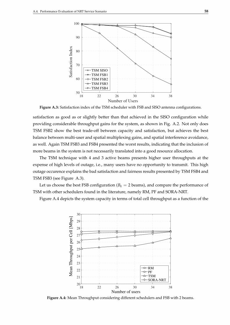
A.4. Performance Evaluation of NRT Service Scenario 58
Number of Users
18 22 26 30 34 38
Sati
sfa
cti
on
In
dex
50
60
70
80
90
100
TSM SISO
TSM FSB1
TSM FSB2
TSM FSB3
TSM FSB4
Figure A.3: Satisfaction index of the TSM scheduler with FSB and SISO antenna configurations.
satisfaction as good as or slightly better than that achieved in the SISO configuration while
providing considerable throughput gains for the system, as shown in Fig. A.2. Not only does
TSM FSB2 show the best trade-off between capacity and satisfaction, but achieves the best
balance between multi-user and spatial multiplexing gains, and spatial interference avoidance,
as well. Again TSM FSB3 and FSB4 presented the worst results, indicating that the inclusion of
more beams in the system is not necessarily translated into a good resource allocation.
The TSM technique with 4 and 3 active beams presents higher user throughputs at the
expense of high levels of outage, i.e., many users have no opportunity to transmit. This high
outage occurence explains the bad satisfaction and fairness results presented by TSM FSB4 and
TSM FSB3 (see Figure A.3).
Let us choose the best FSB configuration (Bk = 2 beams), and compare the performance of
TSM with other schedulers found in the literature, namely RM, PF and SORA-NRT.
Figure A.4 depicts the system capacity in terms of total cell throughput as a function of the
Number of users18 22 26 30 34 38
Mea
n T
hro
ughput
per
Cel
l [M
bps]
20
21
22
23
24
25
26
27
28
29
30
RM PF TSM SORA-NRT
Figure A.4: Mean Throughput considering different schedulers and FSB with 2 beams.

A.4. Performance Evaluation of NRT Service Scenario 59
number of NRT users. As expected, the RM scheduler provides the best results. It is able to
achieve the highest system capacity for all system loads by assigning each beam within the
RBs to the user that can transmit at the highest rate. PF presents good total system throughput
with an almost flat behavior for different traffic loads. Moreover, the SORA-NRT scheduler
presents a reasonable performance in terms of capacity for low and moderate loads because it
tries to satisfy the users as much as possible. However, SORA-NRT achieves very good results
for high offered loads, because it is able to opportunistically exploit the multi-user diversity by
allocating the remaining resources to the flows with the best channel conditions. Finally, TSM
tries to keep the throughput of the satisfied flows as close as possible from each other, which
is not so efficient in terms of system capacity. However, notice that TSM also approaches the
performance of RM when the system load increases. This happens because it is also able to
exploit multi-user diversity in order to achieve higher system capacity.
Figure A.5 depicts the percentage of satisfied users as a function of the system load. TSM
shows the best satisfaction results for all considered system loads, which demonstrates the
advantage of using sigmoidal utility functions when satisfaction maximization is desired. RM
provides an overall degraded QoS because it leaves many users in outage situations. PF and
SORA-NRT also present good satisfaction results, but the latter outperforms the former for
high loads. It is important to highlight the satisfaction gain provided by the proposed TSM
technique compared with SORA-NRT, since the latter was specially designed to provide the
highest satisfaction levels.
Another advantage of the TSM technique is the low computational complexity. Its
complexity is in the same order of PF and lower than SORA-NRT (heuristics). The complexity
of TSM depends only on the calculation of the users’ weights with dimension J, and K sorting
operations of a scheduling metric with dimension J (K and J are the numbers of resources and
users, respectively). The computational complexity of the FSB beamforming is the same for all
schedulers.
Number of users
18 22 26 30 34 38
Sati
sfa
cti
on
In
dex
0
20
40
60
80
100
RM
PF
TSM
SORA-NRT
Figure A.5: Satisfaction index considering different schedulers and FSB with 2 beams.
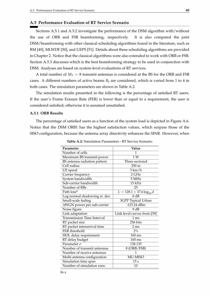
A.5. Performance Evaluation of RT Service Scenario 60
A.5 Performance Evaluation of RT Service Scenario
Sections A.5.1 and A.5.2 investigate the performance of the DSM algorithm with/without
the use of ORB and FSB beamforming, respectively. It is also compared the joint
DSM/beamforming with other classical scheduling algorithms found in the literature, such as
RM [49], MLWDF [50], and UEPS [51]. Details about these scheduling algorithms are provided
in Chapter 2. Notice that the classical algorithms were also extended to work with ORB or FSB.
Section A.5.3 discusses which is the best beamforming strategy to be used in conjunction with
DSM. Analyses are based on system-level evaluations of RT services.
A total number of MT = 8 transmit antennas is considered at the BS for the ORB and FSB
cases. A different numbers of active beams Bk are considered, which is varied from 1 to 4 in
both cases. The simulation parameters are shown in Table A.2.
The simulation results presented in the following is the percentage of satisfied RT users.
If the user’s Frame Erasure Rate (FER) is lower than or equal to a requirement, the user is
considered satisfied; otherwise it is assumed unsatisfied.
A.5.1 ORB Results
The percentage of satisfied users as a function of the system load is depicted in Figure A.6.
Notice that the DSM ORB1 has the highest satisfaction values, which surpass those of the
SISO configuration, because the antenna array directivity enhances the SINR. However, when
Table A.2: Simulation Parameters - RT Service Scenario
Parameter ValueNumber of cells 1Maximum BS transmit power 1 WBS antenna radiation pattern Three-sectoredCell radius 250 mUE speed 3 km/hCarrier frequency 2 GHzSystem bandwidth 5 MHzSub-carrier bandwidth 15 kHzNumber of RBs 25Path lossa L = 128.1 + 37.6 log10 dLog-normal shadowing st. dev. 8 dBSmall-scale fading 3GPP Typical UrbanAWGN power per sub-carrier -123.24 dBmNoise figure 9 dBLink adaptation Link level curves from [39]Transmission Time Interval 1 msRT packet size 256 bitsRT packet interarrival time 2 msFER threshold 2%HOL delay requirement 100 msRT delay budget 100 msParameter σ 138.135Number of transmit antennas 8 (ORB/FSB)Number of receive antennas 1Multi-antenna configuration MU-MISOSimulation time span 15 sNumber of simulation runs 10
In s
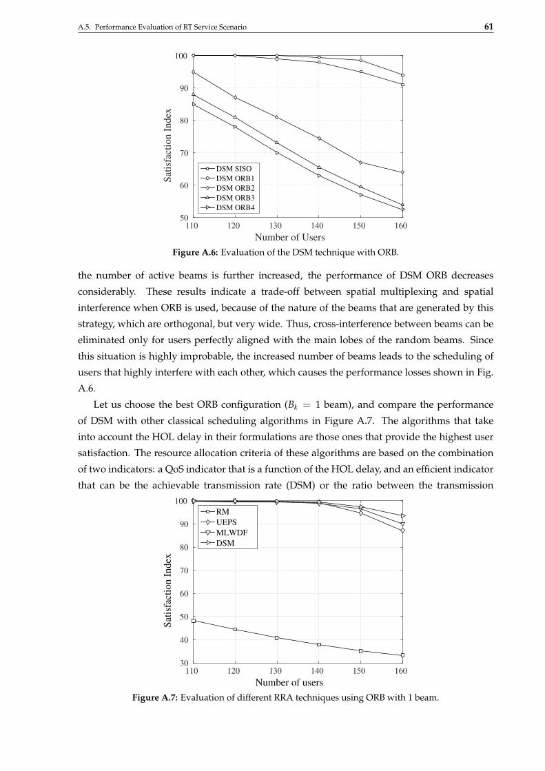
A.5. Performance Evaluation of RT Service Scenario 61
Number of Users
110 120 130 140 150 160
Sati
sfa
cti
on I
nd
ex
50
60
70
80
90
100
DSM SISO
DSM ORB1
DSM ORB2
DSM ORB3
DSM ORB4
Figure A.6: Evaluation of the DSM technique with ORB.
the number of active beams is further increased, the performance of DSM ORB decreases
considerably. These results indicate a trade-off between spatial multiplexing and spatial
interference when ORB is used, because of the nature of the beams that are generated by this
strategy, which are orthogonal, but very wide. Thus, cross-interference between beams can be
eliminated only for users perfectly aligned with the main lobes of the random beams. Since
this situation is highly improbable, the increased number of beams leads to the scheduling of
users that highly interfere with each other, which causes the performance losses shown in Fig.
A.6.
Let us choose the best ORB configuration (Bk = 1 beam), and compare the performance
of DSM with other classical scheduling algorithms in Figure A.7. The algorithms that take
into account the HOL delay in their formulations are those ones that provide the highest user
satisfaction. The resource allocation criteria of these algorithms are based on the combination
of two indicators: a QoS indicator that is a function of the HOL delay, and an efficient indicator
that can be the achievable transmission rate (DSM) or the ratio between the transmission
Number of users
110 120 130 140 150 160
Sati
sfa
cti
on I
nd
ex
30
40
50
60
70
80
90
100
RM
UEPS
MLWDF
DSM
Figure A.7: Evaluation of different RRA techniques using ORB with 1 beam.
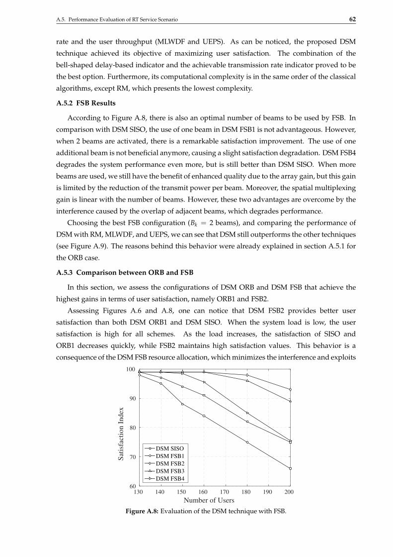
A.5. Performance Evaluation of RT Service Scenario 62
rate and the user throughput (MLWDF and UEPS). As can be noticed, the proposed DSM
technique achieved its objective of maximizing user satisfaction. The combination of the
bell-shaped delay-based indicator and the achievable transmission rate indicator proved to be
the best option. Furthermore, its computational complexity is in the same order of the classical
algorithms, except RM, which presents the lowest complexity.
A.5.2 FSB Results
According to Figure A.8, there is also an optimal number of beams to be used by FSB. In
comparison with DSM SISO, the use of one beam in DSM FSB1 is not advantageous. However,
when 2 beams are activated, there is a remarkable satisfaction improvement. The use of one
additional beam is not beneficial anymore, causing a slight satisfaction degradation. DSM FSB4
degrades the system performance even more, but is still better than DSM SISO. When more
beams are used, we still have the benefit of enhanced quality due to the array gain, but this gain
is limited by the reduction of the transmit power per beam. Moreover, the spatial multiplexing
gain is linear with the number of beams. However, these two advantages are overcome by the
interference caused by the overlap of adjacent beams, which degrades performance.
Choosing the best FSB configuration (Bk = 2 beams), and comparing the performance of
DSM with RM, MLWDF, and UEPS, we can see that DSM still outperforms the other techniques
(see Figure A.9). The reasons behind this behavior were already explained in section A.5.1 for
the ORB case.
A.5.3 Comparison between ORB and FSB
In this section, we assess the configurations of DSM ORB and DSM FSB that achieve the
highest gains in terms of user satisfaction, namely ORB1 and FSB2.
Assessing Figures A.6 and A.8, one can notice that DSM FSB2 provides better user
satisfaction than both DSM ORB1 and DSM SISO. When the system load is low, the user
satisfaction is high for all schemes. As the load increases, the satisfaction of SISO and
ORB1 decreases quickly, while FSB2 maintains high satisfaction values. This behavior is a
consequence of the DSM FSB resource allocation, which minimizes the interference and exploits
Number of Users
130 140 150 160 170 180 190 200
Sati
sfa
cti
on I
ndex
60
70
80
90
100
DSM SISO
DSM FSB1
DSM FSB2
DSM FSB3
DSM FSB4
Figure A.8: Evaluation of the DSM technique with FSB.
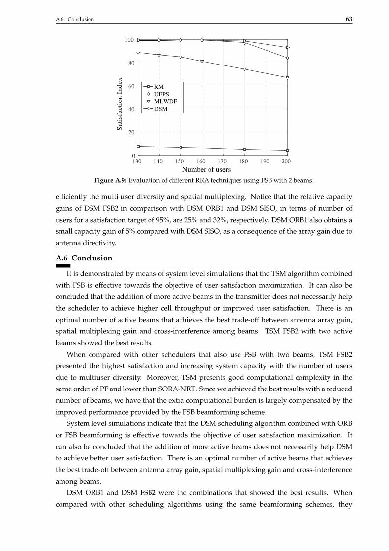
A.6. Conclusion 63
Number of users
130 140 150 160 170 180 190 200
Sati
sfa
cti
on I
nd
ex
0
20
40
60
80
100
RM
UEPS
MLWDF
DSM
Figure A.9: Evaluation of different RRA techniques using FSB with 2 beams.
efficiently the multi-user diversity and spatial multiplexing. Notice that the relative capacity
gains of DSM FSB2 in comparison with DSM ORB1 and DSM SISO, in terms of number of
users for a satisfaction target of 95%, are 25% and 32%, respectively. DSM ORB1 also obtains a
small capacity gain of 5% compared with DSM SISO, as a consequence of the array gain due to
antenna directivity.
A.6 Conclusion
It is demonstrated by means of system level simulations that the TSM algorithm combined
with FSB is effective towards the objective of user satisfaction maximization. It can also be
concluded that the addition of more active beams in the transmitter does not necessarily help
the scheduler to achieve higher cell throughput or improved user satisfaction. There is an
optimal number of active beams that achieves the best trade-off between antenna array gain,
spatial multiplexing gain and cross-interference among beams. TSM FSB2 with two active
beams showed the best results.
When compared with other schedulers that also use FSB with two beams, TSM FSB2
presented the highest satisfaction and increasing system capacity with the number of users
due to multiuser diversity. Moreover, TSM presents good computational complexity in the
same order of PF and lower than SORA-NRT. Since we achieved the best results with a reduced
number of beams, we have that the extra computational burden is largely compensated by the
improved performance provided by the FSB beamforming scheme.
System level simulations indicate that the DSM scheduling algorithm combined with ORB
or FSB beamforming is effective towards the objective of user satisfaction maximization. It
can also be concluded that the addition of more active beams does not necessarily help DSM
to achieve better user satisfaction. There is an optimal number of active beams that achieves
the best trade-off between antenna array gain, spatial multiplexing gain and cross-interference
among beams.
DSM ORB1 and DSM FSB2 were the combinations that showed the best results. When
compared with other scheduling algorithms using the same beamforming schemes, they

A.6. Conclusion 64
presented the highest user satisfaction. When they are compared among each other, it
is concluded that FSB is preferred because it provides the highest gains due to reduced
interference.
The perspectives for future works include
i. evaluation of more realistic scenarios, considering imperfect CSI and inter-cell
interference;
ii. analysis of computational complexity of the proposed algorithms.

Appendix BShifted Log-Logistic Function as a
Generalization of the Logistic Function
The shifted log-logistic function is a generalization of the logistic utility function,
converging to it when the shape parameter tends to zero. To simplify the analysis, we consider
the auxiliary variable, used in Eq. (3.11), as η = 1.
The limit considered is given by
limθ→0
wS-Logj = lim
θ→0
1λ
(1 +
θ(xj[n]− xreqj )
λ
)−1−1/θ
1 +
(1 +
θ(xj[n]− xreqj )
λ
)−1/θ2 (B.1)
Observe that Eq. (B.1) is equivalent to
limθ→0
1λ
(1 +
θ(xj[n]− xreqj )
λ
)−1−1/θ
limθ→0
1 +
(1 +
θ(xj[n]− xreqj )
λ
)−1/θ2 (B.2)
The limit of the numerator can be written as
limθ→0
1λ
(1 +
θ(xj[n]− xreqj )
λ
)−1−1/θ
(B.3)
Consideringθ(xj[n]− xreq
j )
λ=
1y
, the Eq. (B.3) becomes
limθ→0
1λ
(1 +
θ(xj[n]− xreqj )
λ
)−1−1/θ
=

66
limy→∞
1λ
(1 +
1y
)− (xj[n]− xreqj )y
λ =
(1λ· lim
y→∞
(1 +
1y
)y)(xj[n]−xreqj )/λ
=
1λ
e−(xj[n]−xreqj )/λ. (B.4)
Likewise, the limit of the denominator can be written as
limθ→0
1 +
(1 +
θ(xj[n]− xreqj )
λ
)−1/θ2
(B.5)
Regarding again thatθ(xj[n]− xreq
j )
λ=
1y
, the Eq. (B.5) becomes
limy→∞
(1 +
(1 +
1y
)−y(xj[n]−xreqj )/λ
)2
=
(1 + e−(xj[n]−xreq
j )/λ)2
. (B.6)
Combining Eq.(B.4) and Eq.(B.6), the limit initially considered can be written as
1λ
e−(xj[n]−xreqj )/λ(
1 + e−(xj[n]−xreqj )/λ
)2 . (B.7)
Thus, when θ → 0, the shifted log-logistic converges to the logistic function.
Bibliography
[1] T. F. Maciel, “Avaliação de Desempenho de Técnicas de Controle e Atribuição de Potência
para Aumento de Capacidade e Qualidade de Serviço na Rede GSM/EDGE,” Master’s
thesis, Universidade Federal do Ceará, Abril 2004.
[2] 3GPP, “Spatial channel model for multiple input multiple output (MIMO) simulations,”
3rd Generation Partnership Project, TR 25.996 V7.0.0, Jun. 2007.
[3] ——, “Physical layer aspects for evolved universal terrestrial radio access (UTRA),” 3rd
Generation Partnership Project, TR 25.814 V7.1.0, Sep. 2006.
[4] G. Tychogiorgos and K. K. Leung, “Optimization-based Resource Allocation in
Communication Networks,” Computer Networks, vol. 66, pp. 32–45, Jun. 2014.
[5] Ericsson, “Ericsson Mobility Report: On the Pulse of the Networked Society,” Whitepaper,
Nov. 2015.
[6] Cisco, “Cisco Visual Networking Index: Global Mobile Data Traffic Forecast Update,
2014–2019,” Whitepaper, Feb. 2015.
[7] A. Asadi and V. Mancuso, “A Survey on Opportunistic Scheduling in Wireless
Communications,” IEEE Communications Surveys Tutorials, vol. 15, no. 4, pp. 1671–1688,
2013.
[8] F. Capozzi, G. Piro, L. Grieco, G. Boggia, and P. Camarda, “Downlink Packet Scheduling
in LTE Cellular Networks: Key Design Issues and a Survey,” IEEE Communications Surveys
and Tutorials, vol. 15, no. 2, pp. 678–700, Mar. 2013.
[9] R. Knopp and P. Humblet, “Information Capacity and Power Control in Single-Cell
Multiuser Communications,” vol. 01, Jun. 1995, pp. 331–335.
[10] J. Yang, Z. Yifan, W. Ying, and Z. Ping, “Average Rate Updating Mechanism in
Proportional Fair Scheduler for HDR,” in IEEE Global Telecommunications Conference, vol. 6,
Nov 2004, pp. 3464–3466.
[11] R. Kwan, C. Leung, and J. Zhang, “Proportional Fair Multiuser Scheduling in LTE,” IEEE
Signal Processing Letters, vol. 16, no. 6, pp. 461–464, Jun. 2009.
[12] E. Liu and K. Leung, “Proportional Fair Scheduling: Anlytical Insight Under Rayleigh
Fading Environment,” in IEEE Wireless Communications and Networking Conference, 2008,
pp. 1883–1888.
[13] M. Proebster, C. Mueller, and H. Bakker, “Adaptive Fairness Control for a Proportional
Fair LTE Scheduler,” in International Symposium on Personal Indoor and Mobile Radio
Communications, Sep. 2010, pp. 1504–1509.

Bibliography 68
[14] B. Sadiq, S. J. Baek, and G. de Veciana, “Delay-Optimal Opportunistic Scheduling
and Approximations: The Log Rule,” in IEEE International Conference on Computer
Communications, Apr. 2009, pp. 1692–1700.
[15] H. Ramli, R. Basukala, K. Sandrasegaran, and R. Patachaianand, “Performance of Well
Known Packet Scheduling Algorithms in the Downlink 3GPP LTE System,” in IEEE
Malaysia International Conference on Communications, Dec. 2009, pp. 815–820.
[16] D. Skoutas and A. Rouskas, “Scheduling with QoS Provisioning in Mobile Broadband
Wireless Systems,” in European Wireless Conference, Apr. 2010, pp. 422–428.
[17] Y. Zaki, T. Weerawardane, C. Gorg, and A. Timm-Giel, “Multi-QoS-Aware Fair Scheduling
for LTE,” in IEEE Vehicular Technology Conference, May 2011, pp. 1–5.
[18] F. Kelly, “Charging and Rate Control for Elastic Traffic,” European Transactions on
Telecommunications, vol. 8, pp. 33–37, 1997.
[19] G. Song and Y. G. Li, “Cross-layer optimization for OFDM wireless networks - part I:
Theoretical framework,” IEEE Transactions on Wireless Communications, vol. 4, no. 2, pp.
614–624, Mar. 2005.
[20] ——, “Cross-layer optimization for OFDM wireless networks - part II: Algorithm
development,” IEEE Transactions on Wireless Communications, vol. 4, no. 2, pp. 625–634,
Mar. 2005.
[21] M. Fathi and H. Taheri, “Utility-Based Resource Allocation in Orthogonal Frequency
Division Multiple Access Networks,” IET Communications, vol. 4, no. 12, pp. 1463–1470,
Aug. 2010.
[22] R. B. Santos, F. R. M. Lima, and a. F. R. P. C. W. Freitas, “QoS Based Radio
Resource Allocation and Scheduling with Different User Data Rate Requirements for
OFDMA Systems,” in IEEE International Symposium on Personal, Indoor and Mobile Radio
Communications, 2007.
[23] F. R. M. Lima, S. Wänstedt, F. R. P. Cavalcanti, and W. C. Freitas, “Scheduling for
Improving System Capacity in Multiservice 3GPP LTE,” Journal of Electrical and Computer
Engineering, no. 819729, 2010.
[24] E. B. Rodrigues and F. Casadevall, “Adaptive Radio Resource Allocation Framework for
Multi-User OFDM,” in IEEE Vehicular Technology Conference, Apr. 2009, pp. 1–6.
[25] F. R. M. Lima, W. C. Freitas, and F. R. P. Cavalcanti, “Scheduling Algorithm for Improved
System Capacity of Real-Time Services in 3GPP LTE,” in XXVII Telecommunications
Brazilian Symposium - SBrT, Oct. 2009.
[26] E. B. Rodrigues, F. R. M. Lima, T. F. Maciel, and F. R. P. Cavalcanti, “Maximization of
User Satisfaction in OFDMA Systems Using Utility-Based Resource Allocation,” Wireless
Communications and Mobile Computing, pp. 1–17, 2014.

Bibliography 69
[27] E. B. Rodrigues, F. H. C. Neto, T. F. Maciel, F. R. M. Lima, and F. R. P. Cavalcanti,
“Utility-based scheduling and fixed switching beamforming for user satisfaction
improvement in OFDMA systems,” in Procedings of the European Wireless Conference, May
2014, pp. 1–6.
[28] E. B. Rodrigues, F. H. C. Neto, T. F. Maciel, and F. R. P. Cavalcanti, “Utility-Based
Resource Allocation with Spatial Multiplexing for Real Time Services in Multi-User OFDM
Systems,” in Vehicular Technology Conference (VTC Spring), May 2014, pp. 1–5.
[29] R. Bosisio and U. Spagnolini, “On the Sum-Rate of Opportunistic Beamforming
Schemes with Multiple Antennas at the Receiver,” in IEEE International Conference on
Communications, 2007, pp. 1048–1053.
[30] R. Bosisio, J. L. Vicario, C. Anton-Haro, and U. Spagnolini, “The Effect of Imperfect
Feedback on Broadcast Opportunistic Beamforming Schemes,” in European Wireless
Conference, April 2006, pp. 1–7.
[31] J. L. Vicario, “Antenna Selection Techniques in Single- and Multi-User Systems: a
Cross-Layer Approach,” Ph.D. dissertation, Universitat Politecnica de Catalunya, Jun.
2006.
[32] V. F. Monteiro, D. A. Sousa, F. H. C. Neto, E. B. Rodrigues, T. F. Maciel, and F. R. P.
Cavalcanti, “Throughput-Based Satisfaction Maximization for a Multi-Cell Downlink
OFDMA System Considering Imperfect CSI,” in Telecommunications Brazilian Symposium
(SBrT), Sep. 2015.
[33] N. Bao, J. Li, W. Xia, and L. Shen, “QoS-Aware Resource Allocation Algorithm for
OFDMA-WLAN Integrated System,” in IEEE Wireless Communications and Networking
Conference, Apr. 2013, pp. 807–812.
[34] I. Wong and B. Evans, “Optimal Resource Allocation in the OFDMA Downlink with
Imperfect Channel Knowledge,” IEEE Transactions on Communications, vol. 57, no. 1, pp.
232–241, January 2009.
[35] R. Aggarwal, M. Assaad, C. Koksal, and P. Schniter, “Joint Scheduling and
Resource Allocation in the OFDMA Downlink: Utility Maximization Under Imperfect
Channel-State Information,” IEEE Transactions on Signal Processing, vol. 59, no. 11, pp.
5589–5604, Nov 2011.
[36] S. Stefanatos and N. Dimitriou, “Downlink OFDMA Resource Allocation Under Partial
Channel State Information,” in IEEE International Conference on Communications, June 2009,
pp. 1–5.
[37] Z. Wang and L. Liu, “Adaptive Resource Management for Downlink OFDMA System with
Imperfect CSI,” Electronics Letters, vol. 50, no. 7, pp. 554–556, Mar. 2014.
Bibliography 70
[38] M. George and R. Koilpillai, “Fairness-Based Resource Allocation in OFDMA Downlink
with Imperfect CSIT,” in International Conference on Wireless Communications Signal
Processing, Oct 2013, pp. 1–6.
[39] C. Mehlführer, M. Wrulich, J. C. Ikuno, D. Bosanska, and M. Rupp, “Simulating
the Long Term Evolution Physical Layer,” in Procedings of the European Signal
Processing Conference, Glasgow, Scotland, August 2009. [Online]. Available: http:
//publik.tuwien.ac.at/files/PubDat_175708.pdf
[40] J. C. Ikuno, M. Wrulich, and M. Rupp, “System Level Simulation of LTE Networks,” in
Proceedings of the IEEE Vehicular Technology Conference (VTC), May 2010, pp. 1–5.
[41] T. F. Maciel, “Suboptimal Resource Allocation for Multi-User MIMO-OFDMA Systems,”
Ph.D. dissertation, Technische Universität Darmstadt, Darmstädter Dissertationen D17,
Sep. 2008.
[42] T. S. Rappaport, Wireless Communications: Principles and Practice, 2nd ed. Prentice Hall,
2002.
[43] 3GPP, “Deployment aspects,” 3rd Generation Partnership Project, Tech. Rep. TR 25.943
V9.0.0, Dec. 2009.
[44] F. Gunnarsson, M. Johansson, A. Furuskar, M. Lundevall, A. Simonsson, C. Tidestav,
and M. Blomgren, “Downtilted Base Station Antennas - A Simulation Model Proposal
and Impact on HSPA and LTE Performance,” in IEEE Vehicular Technology Conference,
September 2008, pp. 1–5.
[45] R. Batista, T. Maciel, Y. Silva, and F. Cavalcanti, “Impact Evaluation of Imperfect CSI on
the Performance of Downlink CoMP Systems,” in Brazilian Telecommunications Symposium,
Sep. 2011, pp. 1–5.
[46] 3GPP, “Evolved Universal Terrestrial Radio Access (E-UTRA); physical layer procedures,”
3rd Generation Partnership Project, TS 36.213 V8.6.0, Mar. 2009.
[47] P. Ameigeiras, Y. Wang, J. Navarro-Ortiz, P. E. Mogensen, and J. M. Lopez-Soler,
“Traffic Models Impact on OFDMA Scheduling Design,” EURASIP Journal on Wireless
Communications and Networking, pp. 1–13, Feb. 2012.
[48] 3GPP, “Evolved universal terrestrial radio access (E-UTRA); further advancements for
E-UTRA physical layer aspects,” 3rd Generation Partnership Project (3GPP), TR 36.814,
Mar. 2010. [Online]. Available: http://www.3gpp.org/ftp/Specs/html-info/36814.htm
[49] J. Jang and K. B. Lee, “Transmit Power Adaptation for Multiuser OFDM Systems,” IEEE
Journal on Selected Areas in Communications, vol. 21, no. 2, pp. 171–178, Jan. 2003.
[50] M. Andrews, K. Kumaran, K. Ramanan, A. Stolyar, P. Whiting, and R. Vijayakumar,
“Providing Quality of Service over a Shared Wireless Link,” IEEE Communications
Magazine, vol. 32, no. 2, pp. 150–154, Jun. 2001.

Bibliography 71
[51] S. Ryu, B. Ryu, H. Seo, and M. Shin, “Urgency and efficiency based wireless downlink
packet scheduling algorithm in OFDMA system,” in IEEE Vehicular Technology Conference,
vol. 3, May 2005, pp. 1456–1462.
[52] Z. Jiang and Y. G. Li, “Max-Utility Wireless Resource Management for Best-Effort Traffic,”
IEEE Transactions on Wireless Communications, vol. 4, no. 1, pp. 100–111, jan 2005.
[53] H. Rinne, Taschenbuch der Statistik. Verlog Harri Deutsch, 2008.
[54] T. F. Maciel, W. C. Freitas, and F. R. P. Cavalcanti, “Joint Opportunistic Beamforming and
Subcarrier Assignment for Maximization of User Satisfaction in OFDMA Systems,” in
IEEE Vehicular Technology Conference, Sep. 2010.