using semi-variance image texture statistics to model ...lewang/pdf/lewang_sample10.pdf · a...

Introduction

Knowledge of the size and distribution of human population is essential for understanding and responding to

many social, political, economical, and envi-ronmental problems (Liu et al 2006). In the United States, the decennial census is the pri-mary source of demographic data. Although the U.S. Census Bureau conducts census surveys at the household level, the data are released only by aggregated enumeration units because of confidentiality issues and administrative pur-poses. Researchers may encounter two problems when using aggregated census data to conduct research. The first problem is associated with carto-graphic visualization of population density. Choropleth mapping of population density creates the impression that population density is uniform within census units. This may be acceptable when the mapping area consists of a large number of units and the map is gener-ated to visualize the overall trend of population variation. However, when the mapping area only consists of a few census units there may be a

Using Semi-variance Image Texture Statistics to Model Population Densities

Shuo-sheng Wu, Xiaomin Qiu, and Le WangABSTRACT: This study presents a method to model population densities by using image texture statistics of semi-variance. In a case study of the City of Austin, Texas, we first selected sample census blocks of the same land use to build population models by land use. Regression analyses were conducted to infer the relationship between block population densities and image texture statistics of the semi-variance. We then applied the population models to an area of 251 blocks to estimate populations for within-blocks land-use areas while maintaining census block populations. To assess the proposed method, the same analysis was performed while census block-group populations were maintained, and the aggregated block populations were compared with original census block populations. We also tested a conventional land-use-based dasymetric mapping method with pre-calculated population densities for land uses. The results show that our approach, which is based on initial land-use stratification and further image-texture statistical modeling of population, has higher accuracy statistics than the conventional land-use-based dasymetric mapping method.

KEYWORDS: Dasymetric mapping, population density, population disaggregation

Cartography and Geographic Information Science, Vol. 33, No. 2, 2006, pp. 127-140

need to further delineate different population density zones within the units for better visual-ization of population distribution. Specifically, a census unit may contain inhabited and uninhab-ited areas, residential and non-residential land use, and areas of different population densities, particularly in suburban or rural areas where population is sparse. Therefore, for the purpose of visualizing within-unit population distribu-tion, in contrast to visualizing the differences between units, population density maps should, whenever possible, try to map where people actually live. Accordingly, methods are needed to delineate different population density zones within census units.

The second problem for researchers using census population data is that they may need to estimate population counts for areas not coinciding with boundaries of census units. For example, a subdivision for a proposed redevelopment project does not always have the same boundaries as do the census units, yet developers may need to estimate how many people live in the subdivision for cost and benefit analysis. Watersheds generally do not have the same boundaries as the census units, yet researchers may need to estimate watershed populations for environmental impact assessments. City planners may need to estimate populations within a half mile buffer of a proposed railroad route or a proposed landfill site to estimate how many local residents would be affected by the

Shuo-sheng Wu, Xiaomin Qiu, and Le Wang, Department of Geography, Texas State University-San Marcos, 601 University Drive, San Marcos, Texas 78666-4616. Phone: 512-785-7194. E-mail: <{sw1020}, {xq1001}, {lw15}@txstate.edu>.

128 Cartography and Geographic Information Science Vol. 33, No. 2 129

projects. All these examples show that we need methods for estimating populations of arbitrary boundaries.

This study presents a dasymetric mapping method for intra-census-unit population mapping and estimation. We disaggregated census block populations based on their land-use information and image-texture statistics of the semi-variance.

Review of Past Population Estimation Methods in GIS and

Remote SensingAccording to Wu et al. (2005), past studies relevant to population estimation in GIS and remote sensing can be grouped into areal interpolation and statistical modeling, depending on the intended goal and the required information. Areal interpolation studies use census population data as the input and apply certain interpolation techniques to obtain refined population data, usually for the purpose of transforming population data from one set of spatial units to another. In contrast, statistical modeling studies infer a statistical relationship between population and other physical and socio-economic variables, often for the purpose of estimating intercensal populations for urban areas or populations of areas where it is difficult to conduct the census. Nevertheless, some researchers also incorporate statistical modeling into areal interpolation of population (e.g., Harvey 2002b; Yuan et al. 1997).

Areal interpolation of population may be further separated into two categories, depending on whether the interpolation is based on mathematical functions or ancillary information (Wu et al. 2005). For areal interpolation based on mathematical functions there are point-based methods and areal-based methods, depending on whether the population data for computational input are in digital form of points or areas. Examples of point-based interpolation include Martin (1989), Bracken (1991), and Martin (1996). Examples of area-based interpolation include Tobler (1979) and Rase (2001). Areal-based methods usually have the volume-preserving property, i.e., the summation of interpolated population data to individual census units is the same as the original census unit populations.

Population is related to other information such as land use, transportation, and topography. Ancillary information relevant to population

distribution, therefore, can be used to assist areal interpolation of population. Areal interpolation using ancillary information is referred to as the dasymetric mapping method, and this approach is generally volume preserving (Wu et al. 2005). The most commonly used ancillary information for population interpolation is land use/land cover (LULC) data (e.g., Yuan et al. 1997; Mennis 2003; Holt et al. 2004). Others include topographic data (Wright 1936), election districts demographic data (e.g., Flowerdew and Green 1989; 1991), road network data (e.g., Xie 1995; Reibel and Bufalino 2005; Hawley and Moellering 2005), and remote sensing image spectral and textural statistics (Harvey 2002b).

Land use/land cover-based dasymetric mapping assumes the same population densities for the same LULC classes and redistributes census populations to land use areas. The population densities for different land-use classes can be determined from sampling (e.g., Mennis 2003), from regression analysis (e.g., Yuan et al. 1997; Langford et al. 1991), or based on the domain knowledge of researchers (e.g., Eicher and Brewer 2001). Regression analysis seems to provide a more objective approach since population density measures are derived based on the entire land-use and population dataset.

Land use/land cover data are usually derived from remote sensing images through digital image classification. Due to the difficulty of classifying detailed categories of urban land use from remote sensing images (Wu et al. 2006), remote sensing-derived LULC data only provide general categories of urban land use (e.g., residential vs. non-residential) as the ancillary information for population interpolation. Compounded with the errors associated with digital image classification, LULC-based dasymetric mapping for urban areas always has a degree of error. Nevertheless, if detailed and accurate urban land-use data are available, e.g., data of single family, multi-family, industrial, and commercial land uses, then population interpolation based on the data should be more reliable. Such land-use data are most likely to be obtained through image interpretation and manual digitizing. They are usually in vector format with a high degree of precision.

Another category of literatures relevant to popula-tion estimation is statistical modeling. Depending on the scale of analysis, researchers have used five types of predictor variables in regression analyses of population (Wu et al. 2005), including urban areas (e.g., Tobler 1969; Lo and Welch 1977; Prosperie and Eyton 2000), land-use areas (e.g., Kraus et al. 1974; Weber 1994; Lo 2003), classi-


fied dwelling units count (e.g., Hsu 1971; Lo and Chan 1980; Lo 1989), image pixel statistics (e.g., Webster 1996; Harvey 2002a; Liu et al. 2006), and other physical or socioeconomic characteristics (e.g., Green and Monier 1959; Dobson et al. 2000; Liu and Clarke 2002).

We separated population estimation research in GIS and remote sensing into two categories: areal interpolation and statistical modeling. This notwithstanding, statistical modeling approaches have been used for areal interpolation of population (specifically the dasymetric mapping method) in some studies, in the context of estimating popu-lation densities for land-use classes (e.g., Yuan et al. 1997; Langford et al. 1991; Flowerdew and Green 1989) or estimating population by image pixels (e.g., Harvey 2002b).

Although LULC-based dasymetric mapping is an improvement over traditional choropleth mapping, important variations of population distribution within individual land-use classes may still be ignored. In contrast, Harvey (2002b) disaggregated census populations by pixels using a variety of spectral and textural statistics of remote sensing images. This pixel-based dasymetric mapping allows the mapping of detailed variations of population distribution. Its limitation is that the relationship between population and combinations of image pixel statistics cannot be interpreted. In addition there is the possibility that non-residential land areas have the same image pixel statistics as residential land areas. As a result, assuming people only live on residential land, this complexity would make modeling of population by image pixel statistics less reliable. This study combines the strength of LULC-based and pixel-based dasymetric mapping by modeling population from image pixel statistics for different land uses. In this approach, we can separate residential versus non-residential areas as well as areas of different residential land use classes. Then we can model detailed variations of population distribution from image pixel statistics. The volume-preserving strength of dasymetric mapping method is maintained.

Past studies have indicated a strong relationship between population density and image spectral and texture statistics (Lo 1995; Webster 1996; Harvey 2002a). Texture statistics from remotely sensed images measure the degree of spectral variation between pixels and, therefore, indicate the degree of landscape heterogeneity for a given area. For example, residential areas with small houses and small distances between houses rep-resent more heterogeneous landscape and usually have higher values of image texture statistics, such

as variance, standard deviation, and entropy. In contrast, residential areas with large houses and long distances between houses represent more homogeneous landscape and usually have lower values of image texture statistics (Bian and Xie 2004; Liu et al 2006; Wu et al. 2006).

In this study, we used the texture statistic of semi-variance to correlate with population densities. Semi-variance statistics for an area are calculated as half the average of the squared difference between paired pixel values separated at a certain distance, called the lag. The mathemati-cal function of semi-variance, γ(h), separated by a lag, h, can be expressed as:

where: Nh = the number of paired pixels separated by lag h; and zi, zi+h = values of a pair of pixels separated by lag h.

A graph of semi-variance against the lag is called the variogram. The variogram is usually fitted with a mathematical model to indicate the extent of spatial autocorrelation across space, or the degree of landscape heterogeneity at certain lag-scales. As the lag increases, the semi-variance generally becomes larger. At a certain distance, called the range, the semi-variance reaches its limit, called the sill. The range represents the limit of spatial dependence and indicates the distance over which the values would be similar (Burrough and McDonnell 1998).

In this study, semi-variance is used to indicate the degree of landscape heterogeneity, in a way to that of other image texture statisitcs. The advantage of the semi-variance is its ability to indicate landscape heterogeneity at different scales. Common texture statistics, such as variance and standard deviation, only give us an average measure across scales. We expect population density would better correlate to image texture statistics at certain scales.

A Case Study of Austin, TexasThe City of Austin, the capital of Texas, provides a suitable environment to explore the proposed census population interpolation method. With a land area of approximately 650 square kilometers in 2005, Austin is not too large and has a variety of land use types. Between 1990 and 2000, the city’s population has grown from 465,622 to 656,562, or 41 percent, with an

(1)


annual growth rate of 3.5 percent. The annual growth rate between years 2000 and 2005 was approximately 1.2 percent (COA 2005). The city plans to maintain an annual growth rate between 1.20 percent and 2.00 percent for the next thirty years.

There are two stages in our population disaggregation. In the first stage, we selected sample census blocks of the same residential land-use classes around the city to build regression models between block population density and semi-variance statistics calculated within blocks. Non-residential land-use areas were not considered because it is assumed that people only live in residential areas. Using block-level census data is more appropriate than using other higher-level census data, e.g., block groups and tracts data, because a census block is the smallest census enumeration unit and block-level statistics are suitable for inferring sub-block-level populations.

In the second stage of our analysis, we applied the derived regression model to a study site and estimated population densities for individual land-use areas within blocks. We then calculated and rescaled their populations to maintain the summed populations to blocks.

The Census 2000 block-level population data for the Austin area were obtained from the U.S. Census Bureau’s American FactFinder website (U.S. Census Bureau 2000). Digital aerial photo-graphs and land-use data of the year 2000 were obtained from the City of Austin Neighborhood Planning and Zoning Department (NPZD). The digital orthophotos have a spatial resolution of about 0.61 meters (two feet) and green, red, and near-infrared spectral bands. These high-spatial-resolution images allowed us to identify structures on the ground and have an understanding of how population density related to housing and land-use patterns. When calculating image semi-variance statistics, we resampled the digital orthophotos to approximately five meters (16 feet) of spatial resolution so as to achieve computational efficiency. Compared to Système Probatoire d’Observation de la Terre (SPOT) or Landsat Enhanced Thematic Mapper Plus (ETM+) data used in other dasy-metric studies, the fine resolution images we used allowed us to detect detailed spectral variation between human structures and vegetation through image texture statistics in a complicated urban landscape, and proved to better model popula-tion densities.

The year 2000 land-use data are in a vector poly-gon format and have 13 categories (Table 1). The NPZD generated the data based on the geography

of Travis Central Appraisal District (TCAD) tax parcel polygons and land-use information from different sources. Digital infrared and panchromatic aerial photos were the primary sources used to determine land use through visual interpretation (COA 2000). Other sources of land-use informa-tion include historical land-use data, the TCAD appraisal record, and the land development record. The NPZD also performed quality control mea-sure by field checks. The land-use data are used to select residential land-use blocks for building population density models by different residential land-use types. As the land-use data are at the tax parcel level, generally much smaller than census blocks, the data were considered accurate for the purposes of this study.

There are not many large lot single-family and mobile homes land-use areas in Austin; these two categories were thus combined with the single-family land-use category. We only created a single-family land-use model and a multi-family land-use model for inferring block-level population densities.

To build regression models between block popula-tion density and image statistics, we first selected 120 and 100 sample census blocks that are entirely within, respectively, single- and multi-family land use. The sample blocks represent various housing patterns for the same land use in the Austin area. The population densities for individual sample blocks were then calculated by dividing block populations with block areas. We calculated the image texture statistics of semi-variance for sample blocks. A visual basic program was written in the ArcGIS® ArcObjects (Burke 2003) programming environment to calculate the semi-variance of paired image pixel values that were separated at lag distance, based on pixel size within individual sample block areas. We used the near-infrared band of the digital orthophotos to calculate semi-variance statistics because a preliminary analysis indicates that population density is more related to the semi-variance statistics from the infrared band than from other bands. The infrared band shows more contrast between vegetation and human structures, which is relevant to variations of population densities.

We calculated the semi-variance at lag 2 pixels to lag 50 pixels for sample blocks and generated corresponding variograms to investigate which scales of semi-variance to use for population modeling. Figure 1 shows the variograms for 120 single-family sample blocks, and Figure 2 shows the variograms for 100 multi-family sample blocks. One can see that, at the same lag, single-family blocks generally have greater semi-variances (note the difference


in vertical scales in the figures) than multi-family blocks. This means that single-family land-use areas have more heterogeneous landscape patterns than

multi-family land-use areas and, thus, have greater semi-variance texture statistics. Notice that each block has a different variogram pattern. As no single lag is particularly significant for differentiating blocks, we tested semi-variance at all lags in statistical modeling of block population densities.

Our response variable is block population density, and predictor variables are semi-variances at different lags. We first conducted an exploratory analysis examining histograms of all variables one at a time for both the single-family land use model and the multi-family land use model. If it was highly skewed, a logarithmic transformation was applied. The logarithmic transformation had the effect of reducing asymmetry (Chatterjee

et al. 2000). The histograms of block population densities (Figure 3) and all semi-variance variables

Table 1. Year 2000 land-use data of the City of Austin.

Code Major Group Included Uses

50 Large Lot Single-family Single-family homes on lots greater than 10 acres

100 Single-family Single-family detached, Two-Family Attached

113 Mobile homes Mobile homes

200 Multi-family Three/Fourplex, apartment/condo, group quarters, retirement

300 CommercialRetail and general merchandise, apparel and accessories, furniture and home furnishings,

grocery and food sales, eating and drinking, auto related, entertainment, personal services, lodgings, building services

400 Office Administrative offices, financial services (banks), medical offices, research and development

500 Industrial Manufacturing, warehousing, equipment sales and service, recycling and scrap, animal handling

560 Mining Resource extraction, quarries

600 CivicSemi-institutional housing, hospital, government services, educational facilities, meeting and

assembly facilities, cemeteries, day care facilities

700 Open SpaceParks, recreational facilities, golf courses, rreserves and protected areas, water drainage areas

and detention ponds

800 TransportationRailroad facilities, transportation terminal, aviation facilities, parking facilities, right-of-way and

traffic islands

860 Right-of-way Right-of-way and traffic islands

870 Utilities Utility services, radio towers, communication service facilities, water/wastewater facilities

900Undeveloped/

RuralRural uses, vacant land, land under construction

940 Water Inundated areas such as lakes and rivers where delineated

999 Unknown a lot requiring further information to determine how it is used

Figure 1. Variograms for single-family census blocks.


in both land use models are not highly skewed and were not transformed.

We further examined pairwise scatter plots to explore the relationships between block population densities and semi-variance variables, as well as between the semi-variance variables. Figure 4 shows that semi-variances at different lags are highly correlated, which suggested a multi-collinear-ity problem. Nevertheless, we tested all semi-variances in regression analysis in order to investigate how population densities are related to semi-variances at different scales and to build a model with the best predictive power.

Figure 4 also shows that population densities do not have linear relation-ships with individual semi-variance variables. However, we cannot conclude that there is no statistical relationship between population densities and combinations of semi-variance variables. In addition, due to the simplicity of linear regres-sion models and the ease with which they can be interpreted, we hypothesized a linear relationship between population densities and combinations of semi-variance variables. We then conducted a standard statistical regression analysis.

We used the backward elimination procedure to find appropriate combinations of variables. In the procedure, the regression with the full variable set is calculated first, and insignificant variables are removed in turn. In this way, the multi-col-linearity problem can be handled better than with the forward selection procedure and the stepwise method. The final models from backward elimina-tion retained seven semi-variances as the predictor variables for the single-family model and eight semi-variances for the multi-family model:

Figure 2. Variograms for multi-family census blocks.

Figure 3. Histograms of block population densities for (a) single-family and (b) multi-family census blocks.


PDS = 1185 + 2.1*S1 – 2.4*S2 + 1.9*S3 – 0.6*S4 + 1.0*S5 – 1.1*S6 +0.1*S7 (2)

where: PDS = block population densities for the single- family land use model; and M1 to M8 =semi-variances at lag 2, lag 6, lag 8 lag 14, lag 26, lag 28, and lag 46, respectively. PDM = 0.5 – 3.6*M1 + 6.0*M2 – 4.0*M3 + 2.7*M4 – 2.7*M5 +2.3*M6 – 4.7*M7 +2.8*M8 (3)where: PDM = block population densities for the multi- family land use model; and M1 to M8 = semi-variances at lag 2, lag 6, lag 8, lag 26, lag 28, lag 44, lag 48, and lag 50, respectively.

The fit indices, R2, were 0.72 and 0.67 for single-family and multi-family land use models, respectively, indicating that approximately 72 percent and 67 percent of the variability in block population densities can be explained by combina-tions of semi-variance variables. The significance values of the F statistic in the ANOVA analysis of variance test were both less than 0.05, indicating that the variation explained by the models was not due to chance.

These results confirm that using a range of scales of semi-variance to model population densities is preferable to using semi-variances at similar scales. In other words, because population densities are related to landscape heterogeneity at different scales, they are better modeled by

different scales of semi-variance. The single-family land-use model predicted population densities better at smaller lags than did the multi-family land-use model. This is probably because single-family land use has smaller building sizes and is more sensitive to spatial statistics at smaller scales. The single-family land-use model also had a higher R2, which indicates that there is a more regular and predictable relationship between landscape heterogeneity and population densities in single-family land use than in multi-family land use.

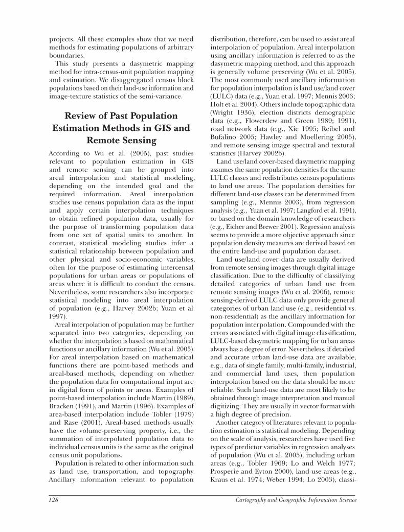
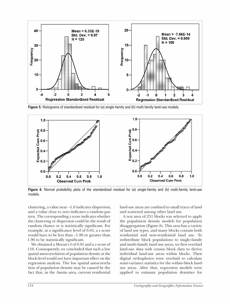
We further verified the standard regression assumptions of linearity, normality of errors, zero mean of errors, constant variance of errors, and independence of errors. Graphical methods were used for the tests because of their simplicity and ease of interpretation. The histogram of the standardized residual (Figure 5), the normal prob-ability plot of the standardized residual (Figure 6), and the scatter plot of the standardized residual versus the standardized predicted value (Figure 7) all show that the assumptions were satisfied.

We investigated whether spatial autocorrelation exists in block-level population density, because serious spatial autocorrelation would violate the independence assumptions underlying regression analysis (O’Sullivan and Unwin 2003; Longley et al. 2005). Moran’s I statistic for 7077 blocks in the Austin area was calculated using ArcGIS (Mitchell 2005) in order to determine whether the pattern of block population density is clustered, dispersed, or random. A Moran’s I value near +1.0 indicates

Figure 4. Pairwise scatter plots for (a) single-family and (b) multi-family land use models (Var0 is block population densities, Var1 to Var8 are semi-variances at lag 4 to lag 46 for every 6 lags).


clustering, a value near –1.0 indicates dispersion, and a value close to zero indicates a random pat-tern. The corresponding z score indicates whether the clustering or dispersion could be the result of random chance or is statistically significant. For example, at a significance level of 0.05, a z score would have to be less than –1.96 or greater than 1.96 to be statistically significant.

We obtained a Moran’s I of 0.01 and a z score of 110. Consequently, we concluded that such a low spatial autocorrelation of population density at the block-level would not have important effect on the regression analysis. The low spatial autocorrela-tion of population density may be caused by the fact that, in the Austin area, current residential

land-use areas are confined to small tracts of land and scattered among other land use.

A test area of 251 blocks was selected to apply the population density models for population disaggregation (Figure 8). This area has a variety of land use types, and many blocks contain both residential and non-residential land use. To redistribute block populations to single-family and multi-family land-use areas, we first overlaid land-use data with census block data to derive individual land-use areas within blocks. Then digital orthophotos were overlaid to calculate semi-variance statistics for the within-block land-use areas. After that, regression models were applied to estimate population densities for

Figure 5. Histograms of standardized residual for (a) single-family and (b) multi-family land-use models.

Figure 6. Normal probability plots of the standardized residual for (a) single-family and (b) multi-family land-use models.


those areas. If the estimated population density was negative, it was adjusted to zero, given that population density cannot be negative (e.g., Lo 1995; Harvey 2002a).

We calculated estimated populations for the within-block land-use areas by multiplying their respective areas with their estimated population densities. We then summed the areal populations to census blocks and compared the summed totals with original census block populations to derive their ratios. Finally, population estimates for within-block land-use areas were rescaled to maintain original census block populations.

To visualize the population disaggregation results, a graduated color thematic map of population densities by small land-use areas within blocks was generated (Figure 9). The map revealed detailed variation of population densities within blocks, in contrast to the traditional population density map by census blocks (Figure 10). A single-family land-use area of the map (Figure 11) shows that the map distinguishes three population density zones related to the spatial patterns of houses.

To quantitatively assess the proposed disaggregation approach and compare it with the traditional LULC-based population disaggregation, we performed a population disaggregation test that maintains census block-group

populations instead of block populations. The sum of the block populations thus obtained can be further compared with census block populations for the purpose of accuracy assessment.

The mean absolute relative error (MARE) may be used to compare estimated block populations with original census block populations. The MARE for the 251 blocks in our study was calculated as follows:

Figure 7. Scatter plot of standardized residual versus standardized predicted value for (a) single-family and (b) multi-family land-use models.

Figure 8. The test area in Austin, Texas, for population disaggregation.

(4)


where: Pi = the estimated population for the ith census block; Yi = the census reported population for the ith census block; and m= the number of census blocks under investigation.

The MARE gives an overall estimate of the percentage of original block populations that were under- or over-estimated. This measure was adopted because it is easy to interpret. The MARE for the proposed population disaggregation approach is approximately 11.8 percent, indicating that on average, approximately 12 percent of the original block populations are either over- or under-estimated.

To compare the proposed disaggregation approach with the traditional LULC-based population disaggregation, we first calculated the average population densities for single-family land use at 2.94 persons per 1000 square meters and for multi-family land use at 10.40 persons per 1000 square meters. Then we estimated populations for within-block land-use areas based on population density. The areal populations were further rescaled to maintain census block-group populations. Lastly, The MARE was calculated to assess the extent to which the aggregated block populations deviate from census block populations.

The MARE was approximately 19.2 percent, which is much higher than the MARE obtained with our disaggregation method. We therefore concluded that initial land-use stratification and further texture statistical modeling has a higher overall accuracy than the traditional LULC-based population disaggregation. Modeling population densities by image semi-variance statistics without land-use stratification had a MARE of approximately 14.6 percent, further indicating the advantage of our method.

We investigated the distribution of estimation errors and whether the errors are spatially correlated

by calculating the relative error for an ith census block (REi):

where: Yi = the census population for the ith census block;

Figure 9. Remodeled population density map by small land-use areas within blocks.

Figure 10. Traditional map of population density by census blocks.

(5)


Pi = the estimated population for the ith census block; m = the number of census blocks under investigation; andREi = the relative error for the ith census block.

The relative errors for the 251 blocks ranged from -9.8 percent to 98.2 percent. They are skewed to the right (Figure 12), indicating that most block populations were over-estimated. The cause of this is not clear. The relative errors of block population estimates mapped in Figure 13 do not show whether the errors are spatially correlated. The 0.03 Moran’s I statistic we calculated, and the corresponding z score of 6, both indicate that the errors were not spatially autocorrelated.

DiscussionWe only built a single-family and a multi-family land-use model for the Austin area. More levels of model stratification may be needed for other urban areas in order to model subtypes of

residential land use that are significant to those area, e.g., mobile home land use and large-lot single-family land use.

Regression models derived in this study may not be directly applicable to other urban areas, because housing geography and the corresponding image texture statistics vary considerably among U.S. cities. A more appropriate strategy would thus be to develop a new population density model for the area of interest, using the multi-lag semi-variance statistics and land-use stratification approach we proposed.

A limitation is that this method requires detailed urban land-use data for model stratification. The data quality/accuracy issues that may affect popula-tion density estimation using our method include miscounting of the census data on houses under construction or otherwise unoccupied, time dif-ference between census and image acquisition, and outdated land- use data. However, since our final population disaggregation by small within-block land-use areas is constrained by census

Figure 11. Inset of Figure 9, remodeled population density map by small land-use areas.


block population totals, all errors are also constrained and would not have a significant impact on population estimation for large areas that cover numerous blocks (Fisher and Langford 1996).

ConclusionIn this paper we present an improved dasy-metric mapping method for remodeling census populations. The method models areal population densities from texture statis-tics of remote sensing images within the same land-use stratification, while maintaining census block population totals, as is the case in common dasymetric mapping approaches. The proposed approach combines the strength of LULC- and pixel-based dasymetric map-ping. The results show improved accuracies compared to either LULC- or pixel-based

approaches using the same parameters. The proposed population estimation method may be applied to estimate intercensal populations in conjunction with the analysis of remote sens-ing data taken during the current year.

Land use/land cover stratification combined with pixel-based dasymetric mapping allows reliable population estimation at large scales, particularly for urban areas. The refined population maps provide a more accurate representation of population distribution than conventional maps

Figure 13. Spatial distribution of relative errors.

of population density by census blocks or land-use types. The disaggregated populations may allow for population estimation within arbitrary boundaries, particularly when integrating with other spatial data of different spatial units, such as watersheds or ecological zones.

Future research may incorporate other population-relevant variables into the regression models, such as building heights and other socio-economic statistics. However, for the models to be practical, their parameters should be readily available or easily extractable from remote sensing images. The presented method utilizes image texture statistics and existing land-use data to remodel census population, which suggests that it is feasible for fine-scale population estimation.

REFERENCESBian, L., and Z. Xie. 2004. A spatial dependence

approach to retrieving industrial complexes from digital images. Professional Geographer 56(3): 381-93.

Bracken, I. 1991. A surface model approach to small area population estimation. Town Planning Review 62(2): 225–37.

Burke, R. 2003. Getting to know ArcObjects: Programming ArcGIS with VBA. Redlands, California: ESRI Press.

Burrough, P.A., and R. McDonnell. 1998. Principles of

Figure 12. Histogram of relative errors.


geographical information systems. New York, New York: Oxford University Press.

Chatterjee, S., A.S. Hadi, and B. Price. 2000. Regression analysis by example. New York, New York: Wiley.

COA (City of Austin). 2000. Land use survey methodology. [http://www.ci.austin.tx.us/landuse/survey.htm; accessed March 22, 2006].

COA (City of Austin). 2005. City of Austin demographics. [http://www.ci.austin.tx.us/census/; accessed March 22, 2006].

Dobson, J.E., E.A. Bright, P.R. Coleman, R.C. Durfee, and B.A. Worley. 2000. LandScan: A global population database for estimating populations at risk. Photogrammetric Engineering and Remote Sensing 66(7): 849-57.

Eicher, C. L., and C. A. Brewer. 2001. Dasymetric mapping and areal interpolation: Implementation and evaluation. Cartography and Geographic Information Science 28(2): 125–38.

Fisher, P. F., and M. Langford. 1996. Modeling sensitivity to accuracy in classified imagery: A study of areal interpolation by dasymetric mapping. Professional Geographer 48(3): 299–309.

Flowerdew, R., and M. Green. 1989. Statistical methods for inference between incompatible zonal systems. In: Goodchild, M., and S. Gopal (eds), Accuracy of spatial databases. London, U.K.: Taylor and Francis. pp. 239-47.

Flowerdew, R., and M. Green. 1991. Data integration: Statistical methods for transferring data between zonal systems. In: Masser, I., and M. Blakemore (eds), Handling geographical information: Methodology and potential applications. New York, New York: Wiley. pp. 38–54.

Green, N.E., and R.B. Monier. 1959. Aerial photographic interpretation of the human ecology of the city. Photogrammetric Engineering 25: 770-3.

Harvey, J.T. 2002a. Estimating census district populations from satellite imagery: Some approaches and limitations. International Journal of Remote sensing 23(10): 2071–95.

Harvey, J.T. 2002b. Population estimation models based on individual TM pixels. Photogrammetric Engineering and Remote Sensing 68(11): 1181-92.

Hawley, K., and H. Moellering. 2005. A comparative analysis of areal interpolation methods. Cartography and Geographic Information Science 32(4): 411-23.

Holt, J. B., C. P. Lo, and T. W. Hodler. 2004. Dasymetric estimation of population density and areal interpolation of census data. Cartography and Geographic Information Science 31(2): 103-21.

Hsu, S.Y. 1971. Population estimation. Photogrammetric Engineering 37: 449-54.

Kraus, S.P., L.W. Senger, and J.M. Ryerson. 1974. Estimating population from photographically determined residential land use types. Remote Sensing of Environment 3(1): 35-42.

Langford, M., D. J. Maguire, and D. J. Unwin. 1991. The areal interpolation problem: Estimating population using remote sensing in a GIS

framework. In: Masser, I., and M. Blakemore (eds), Handling geographical information: Methodology and potential applications. New York, New York: Wiley. pp. 55–77.

Longley, P., M. Goodchild, D. Maguire, and D. Rhind. 2005. Geographic information systems and science. New York, New York: Wiley.

Liu, X., and K.C. Clarke. 2002. Estimation of residential population using high resolution satellite imagery. In: Maktav, D., C. Juergens, and F. Sunar-Erbek (eds), Proceedings of the 3rd Symposium in Remote Sensing of Urban Areas, June 11-13, 2002. Istanbul, Turkey: Istanbul Technical University Press. pp. 153-60.

Liu, X., K.C. Clarke, and M. Herold. 2006. Population density and image texture: A comparison study. Photogrammetric Engineering & Remote Sensing 72(2): 187-96.

Lo, C. P. 1989. A raster approach to population estimation using high-altitude aerial and space photographs. Remote Sensing of Environment 27, no. 1: 59-71.

Lo, C. P. 1995. Automated population and dwelling unit estimation from high-resolution satellite images–A GIS approach. International Journal of Remote Sensing 16(1): 17-34.

Lo, C. P. 2003. Zone-based estimation of population and housing units from satellite-generated land use/land cover maps. In: Mesev, V. (ed.), Remotely sensed cities. New York, New York: Taylor & Francis. pp. 157-80.

Lo, C.P., and H.F. Chan. 1980. Rural population estimation from aerial photographs. Photogrammetric Engineering and Remote Sensing 46(3): 337-45.

Lo, C.P., and R. Welch. 1977. Chinese urban population estimates. Annals of the Association of American Geographers 67(2): 246-53.

Martin, D. 1989. Mapping population data from zone centroid locations. Transactions of the Institute of British Geographers 14(1): 90-7.

Martin, D. 1996. An assessment of surface and zonal models of population. International Journal of Geographical Information Systems 10(8): 973-89.

Mennis, J. 2003. Generating surface models of population using dasymetric mapping. Professional Geographer 55(1): 31-42.

Mitchell, A. 2005. The ESRI guide to GIS analysis. Redlands, California: ESRI Press.

O’Sullivan, D., and D. Unwin. 2003. Geographic information analysis. New York, New York: Wiley.

Prosperie, L., and R. Eyton. 2000. The relationship between brightness values from a nighttime satellite image and Texas county population. Southwestern Geographer 4: 16-29.

Rase, W. 2001. Volume-preserving interpolation of a smooth surface from polygon-related data. Journal of Geographical Systems 3(2): 199-213.

Reibel, M., and M.E. Bufalino. 2005. Street-weighted interpolation techniques for demographic count estimation in incompatible zone systems. Environment and Planning A 37(1): 127-39.

140 Cartography and Geographic Information Science

Tobler, W.R. 1969. Satellite confirmation of settlement size coefficients. Area 1(3): 30-4.

Tobler, W.R. 1979. Smooth pyncophylactic interpolation for geographical regions. Journal of the American Statistical Association 74(367): 519-30.

U.S. Census Bureau. 2000. The U.S. Census American FactFinder. [http://factfinder.census.gov/home/saff/ main.html?_lang=en; accessed August 8, 2005].

Weber, C. 1994. Per-zone classification of urban land use cover for urban population estimation. In: Foody, G. M., and P. J. Curran (eds), Environmental remote sensing from regional to global scales. New York, New York: Wiley. pp. 142-8.

Webster, C. J. 1996. Population and dwelling unit estimation from space. Third World Planning Review 18(2): 155-76.

Wright, J. K. 1936. A method of mapping densities of population. The Geographical Review 26(1): 103-10.

Wu, S., X. Qiu, and L. Wang. 2005. Population estimation methods in GIS and remote sensing: A review. GIScience & Remote Sensing 42(1): 58-74.

Wu, S., B. Xu, and L. Wang. 2006. Urban land use classification using variogram-based analysis with aerial photographs. Photogrammetric Engineering & Remote Sensing 72(7).

Yuan, Y., R. M. Smith, and W.F. Limp. 1997. Remodeling census population with spatial information from LandSat TM imagery. Computers, Environment and Urban Systems 21(3-4): 245-58.

Xie, Y. 1995. The overlaid network algorithms for areal interpolation problem. Computers Environment and Urban Systems 19(4): 287-306.

using semi-variance image texture statistics to model ...lewang/pdf/lewang_sample10.pdf · a...

Documents