using census data, urban land-cover … · dasymetric mapping was performed using the...
TRANSCRIPT
USING CENSUS DATA, URBAN LAND-COVER CLASSIFICATION, AND
DASYMETRIC MAPPING TO MEASURE URBAN GROWTH OF THE
LOWER RIO GRANDE VALLEY, TEXAS
by
Eric Nathaniel Peña
A Thesis Presented to the FACULTY OF THE USC GRADUATE SCHOOL
UNIVERSITY OF SOUTHERN CALIFORNIA In Partial Fulfillment of the
Requirements for the Degree MASTER OF SCIENCE
(GEOGRAPHIC INFORMATION SCIENCE AND TECHNOLOGY)
December 2012
Copyright 2012 Eric Nathaniel Peña
ii
Table of Contents
List of Tables ................................................................................................................................... iv
List of Figures ................................................................................................................................... v
Abstract .......................................................................................................................................... vii
Introduction ..................................................................................................................................... 1
Statement of the Problem ........................................................................................................... 1
Research Questions ..................................................................................................................... 2
Research Objective ...................................................................................................................... 3
Background ...................................................................................................................................... 4
Defining Urban Areas and Urban Growth .................................................................................... 4
Using Census Data to Measure Urban Growth ............................................................................ 7
Using Satellite Remote Sensing Data to Measure Urban Growth ............................................... 9
Dasymetric Mapping .................................................................................................................. 11
Study Area ...................................................................................................................................... 16
Data Collection and Data Preparation ........................................................................................... 18
Population Data ......................................................................................................................... 18
Satellite Imagery ........................................................................................................................ 20
Methodology .................................................................................................................................. 22
Assumptions and Limitations ..................................................................................................... 22
iii
Analysis ...................................................................................................................................... 24
Urban Land-Cover Classification ............................................................................................ 24
Dasymetric Mapping .............................................................................................................. 27
Results ............................................................................................................................................ 28
Population Growth Based on Census Estimates ........................................................................ 28
Land-Cover Classifications ......................................................................................................... 33
Urban Land-Cover Changes ........................................................................................................ 34
Dasymetric Population Distribution ........................................................................................... 36
Discussion and Conclusions ........................................................................................................... 41
Summary of the Work ................................................................................................................ 41
Future Work ............................................................................................................................... 42
Bibliography ................................................................................................................................... 43
iv
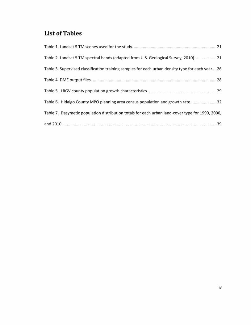
List of Tables
Table 1. Landsat 5 TM scenes used for the study. ......................................................................... 21
Table 2. Landsat 5 TM spectral bands (adapted from U.S. Geological Survey, 2010). .................. 21
Table 3. Supervised classification training samples for each urban density type for each year. .. 26
Table 4. DME output files. ............................................................................................................. 28
Table 5. LRGV county population growth characteristics. ............................................................ 29
Table 6. Hidalgo County MPO planning area census population and growth rate. ...................... 32
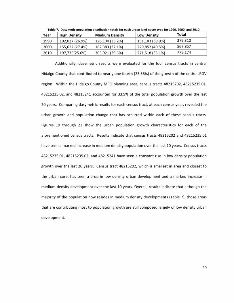
Table 7. Dasymetic population distribution totals for each urban land-cover type for 1990, 2000,
and 2010. ....................................................................................................................................... 39
v
List of Figures
Figure 1. Urban growth categories (adapted from Bhatta, 2010) ................................................... 6
Figure 2. Three population distribution techniques including A, aggregated population by census
enumeration unit, B, binary even distribution into “inhabited” land-use, and C, multi-class
weighted distribution into 3 urban density classes (adapted from Sleeter and Gould, 2007). ..... 12
Figure 3. LRGV counties, metropolitan and micropolitan statistical areas, and urban census
designations (adapated from U.S. Census Bureau, 2011). ............................................................ 17
Figure 4. LRGV 20 year population growth and 10 year projections (adapated from Texas State
Data Center, 2012). ........................................................................................................................ 18
Figure 5. Method of relating census tract population across census years. Census population
counts from 2010 were adjusted to 2000 tract boundaries. 2010 and 2000 census population
counts were then adjusted to 1990 tract boundaries. .................................................................. 19
Figure 6. WRS-2 Path/Row tiles that coincide with the study area. .............................................. 20
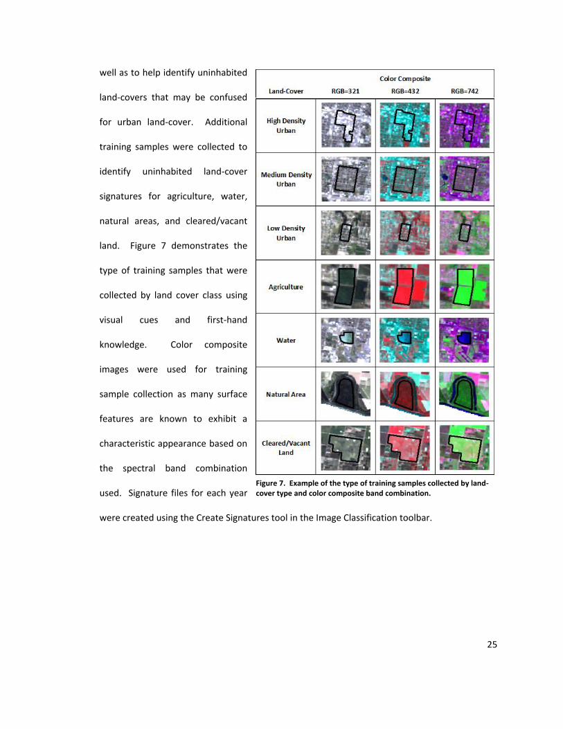
Figure 7. Example of the type of training samples collected by land-cover type and color
composite band combination. ....................................................................................................... 25
Figure 8. Urban land-cover classification methodology. ............................................................... 27
Figure 9. Census tracts with a negative growth rate from 1990 to 2010. Note that population
counts were adjusted to 1990 census boundaries. ....................................................................... 30
Figure 10. Population growth rate by census tract from 1990 to 2010. ....................................... 31
Figure 11. Share of regional growth by census tract from 1990 to 2010. ..................................... 32
Figure 12. 1990 urban land-cover classification. ........................................................................... 33
Figure 13. 2000 urban land-cover classification. ........................................................................... 33

vi
Figure 14. 2010 urban land-cover classification. ........................................................................... 34
Figure 15. 3-class urban land-cover showing decadal changes from 1990 to 2010 for the City of
Mission, TX. .................................................................................................................................... 35
Figure 16. 1990, 2000, and 2010 urban land-cover area and total population counts for the
Hidalgo County MPO planning area. .............................................................................................. 36
Figure 17. Comparison between choropleth and dasymetric population density maps for 1990,
2000, and 2010. ............................................................................................................................. 37
Figure 18. Comparison of 2010 choropleth and dasymetric population density results for census
tract 48215213.02. The dasymetric population density that is highlighted represents the
northern population of the town of Las Milpas, TX. ...................................................................... 38
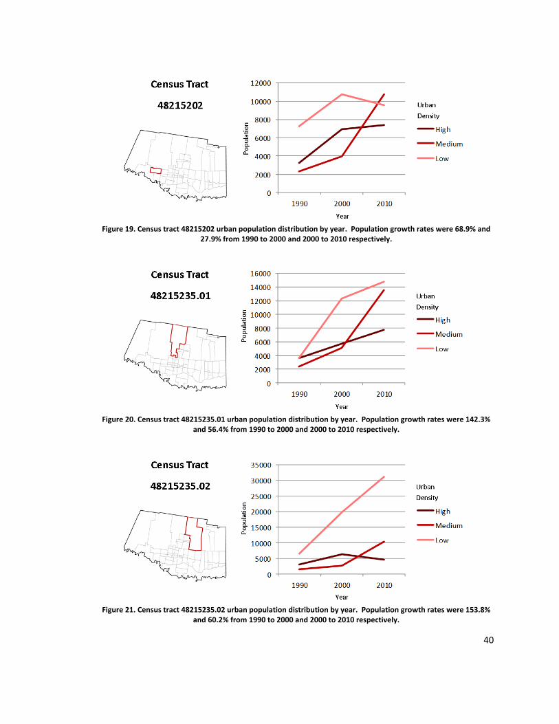
Figure 19. Census tract 48215202 urban population distribution by year. Population growth
rates were 68.9% and 27.9% from 1990 to 2000 and 2000 to 2010 respectively. ........................ 40
Figure 20. Census tract 48215235.01 urban population distribution by year. Population growth
rates were 142.3% and 56.4% from 1990 to 2000 and 2000 to 2010 respectively. ...................... 40
Figure 21. Census tract 48215235.02 urban population distribution by year. Population growth
rates were 153.8% and 60.2% from 1990 to 2000 and 2000 to 2010 respectively. ...................... 40
Figure 22. Census tract 48215241 urban population distribution by year. Population growth
rates were 143.2% and 45.8% from 1990 to 2000 and 2000 to 2010 respectively. ...................... 41
vii
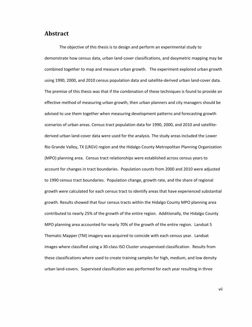
Abstract
The objective of this thesis is to design and perform an experimental study to
demonstrate how census data, urban land-cover classifications, and dasymetric mapping may be
combined together to map and measure urban growth. The experiment explored urban growth
using 1990, 2000, and 2010 census population data and satellite-derived urban land-cover data.
The premise of this thesis was that if the combination of these techniques is found to provide an
effective method of measuring urban growth, then urban planners and city managers should be
advised to use them together when measuring development patterns and forecasting growth
scenarios of urban areas. Census tract population data for 1990, 2000, and 2010 and satellite-
derived urban land-cover data were used for the analysis. The study areas included the Lower
Rio Grande Valley, TX (LRGV) region and the Hidalgo County Metropolitan Planning Organization
(MPO) planning area. Census tract relationships were established across census years to
account for changes in tract boundaries. Population counts from 2000 and 2010 were adjusted
to 1990 census tract boundaries. Population change, growth rate, and the share of regional
growth were calculated for each census tract to identify areas that have experienced substantial
growth. Results showed that four census tracts within the Hidalgo County MPO planning area
contributed to nearly 25% of the growth of the entire region. Additionally, the Hidalgo County
MPO planning area accounted for nearly 70% of the growth of the entire region. Landsat 5
Thematic Mapper (TM) imagery was acquired to coincide with each census year. Landsat
images where classified using a 30-class ISO Cluster unsupervised classification. Results from
these classifications where used to create training samples for high, medium, and low density
urban land-covers. Supervised classification was performed for each year resulting in three
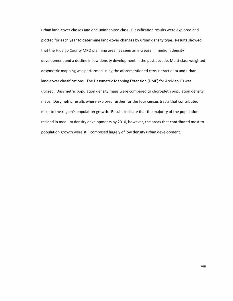
viii
urban land-cover classes and one uninhabited class. Classification results were explored and
plotted for each year to determine land-cover changes by urban density type. Results showed
that the Hidalgo County MPO planning area has seen an increase in medium density
development and a decline in low density development in the past decade. Multi-class weighted
dasymetric mapping was performed using the aforementioned census tract data and urban
land-cover classifications. The Dasymetric Mapping Extension (DME) for ArcMap 10 was
utilized. Dasymetric population density maps were compared to choropleth population density
maps. Dasymetric results where explored further for the four census tracts that contributed
most to the region’s population growth. Results indicate that the majority of the population
resided in medium density developments by 2010, however, the areas that contributed most to
population growth were still composed largely of low density urban development.
1
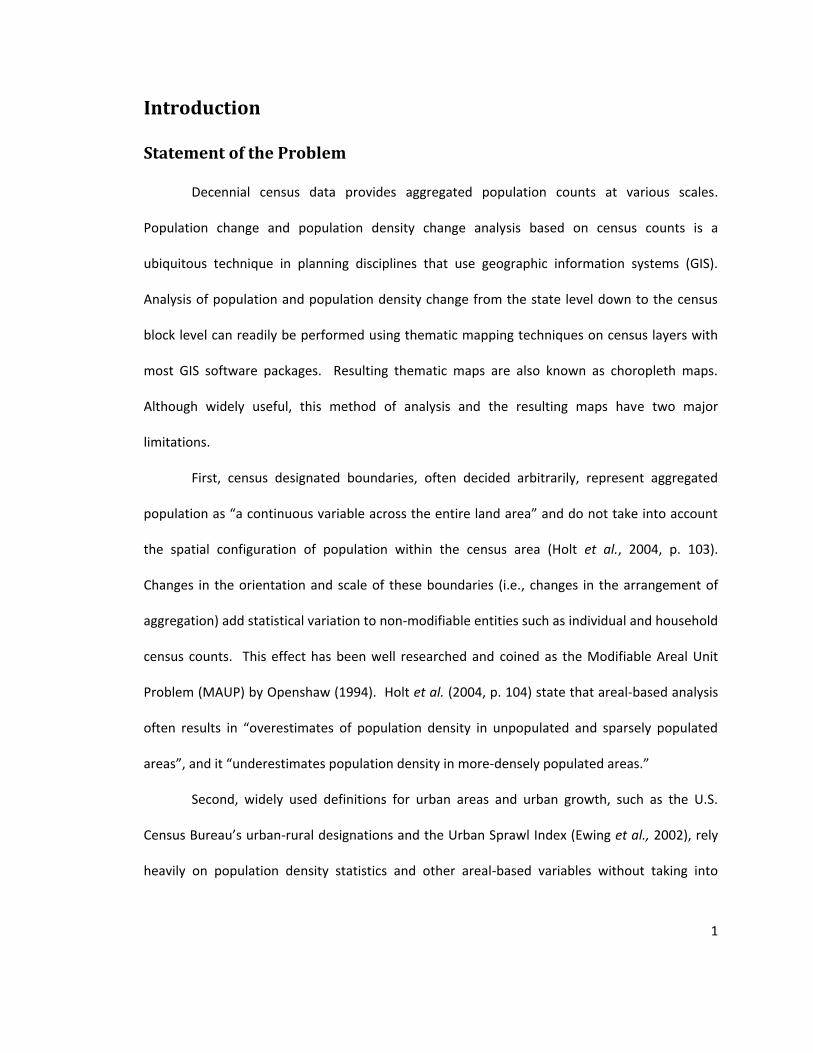
Introduction
Statement of the Problem
Decennial census data provides aggregated population counts at various scales.
Population change and population density change analysis based on census counts is a
ubiquitous technique in planning disciplines that use geographic information systems (GIS).
Analysis of population and population density change from the state level down to the census
block level can readily be performed using thematic mapping techniques on census layers with
most GIS software packages. Resulting thematic maps are also known as choropleth maps.
Although widely useful, this method of analysis and the resulting maps have two major
limitations.
First, census designated boundaries, often decided arbitrarily, represent aggregated
population as “a continuous variable across the entire land area” and do not take into account
the spatial configuration of population within the census area (Holt et al., 2004, p. 103).
Changes in the orientation and scale of these boundaries (i.e., changes in the arrangement of
aggregation) add statistical variation to non-modifiable entities such as individual and household
census counts. This effect has been well researched and coined as the Modifiable Areal Unit
Problem (MAUP) by Openshaw (1994). Holt et al. (2004, p. 104) state that areal-based analysis
often results in “overestimates of population density in unpopulated and sparsely populated
areas”, and it “underestimates population density in more-densely populated areas.”
Second, widely used definitions for urban areas and urban growth, such as the U.S.
Census Bureau’s urban-rural designations and the Urban Sprawl Index (Ewing et al., 2002), rely
heavily on population density statistics and other areal-based variables without taking into
2
account the built environment. Social environments and built environments are not mutually
exclusive though. Social changes (e.g., rural to urban migration, sprawl) influence the built
environment, and in turn, the built environment is an indicator of social elements such as
population density. Weeks et al. (2005, p. 2) simply state it as, “humans transform the
environment, and are then transformed by the new environment.” Weeks et al. (2005, p. 4)
further suggest that “a relatively narrow range of combined values of the built and social
environments would describe a unique set of urban populations.” For this reason urban
measures and urban growth estimates should combine measures from both the social
environment (i.e., census data) and the built environment.
Research Questions
The purpose of this study is to test the utility of census data, satellite-derived land-cover
classifications, and dasymetric mapping techniques to measure urban growth over time. By
comparison to choropleth maps, dasymetric maps greatly reduce statistical variability by
mapping areas of inherent homogeneity in the data (Kimerling et al., 2009; Sleeter and Gould,
2007). Additionally, it is not sufficient to simply consider natural-to-urban land-cover changes as
sprawl. Dasymetric population densities are needed to understand both the social and
landscape changes that are occurring over time. The use of ancillary data such as remotely
sensed land-cover classifications may more accurately map and quantify population density by
distributing population only into areas that can be inferred as populated (i.e., residential,
medium density land-cover). This study addresses the following two main questions:
1. How do census data and satellite-derived urban land-cover classifications
measure urban growth?
3
2. To what extent does the combination of these datasets through dasymetric
mapping enhance the mapping and measurement of population density and
urban growth?
The conclusion is that measures of both the social and built environments are needed for
accurate measurements of urban growth.
Research Objective
The objective of this thesis is to design and perform an experimental study to
demonstrate how census data, urban land-cover classifications, and dasymetric mapping may be
combined to measure and map urban growth. The experiment will explore urban growth using
1990, 2000, and 2010 census population data and satellite-derived urban land-cover data. The
premise of this thesis is that the combination of these techniques provides an effective method
of measuring urban growth, and planners and managers should use them together when
measuring development patterns and forecasting growth scenarios of urban areas. The more
accurate these measurements are, the better the job planners will do in estimating housing
needs, preparing regional transportation plans, assessing the potential impact to the
environment, and designing effective growth strategies.
The study area used for this experiment is the Lower Rio Grande Valley (LRGV) of Texas,
a four county region that has seen substantial growth over the last 20 years. LRGV encompasses
Starr, Hidalgo, Willacy, and Cameron counties, sharing its southern border with Mexico along
the Rio Grande. LRGV is a delta region with agribusiness as the primary economic industry for
the last 100 years (Vigness and Odintz, 2011). In the latter half of the 20th century the region has
witnessed a merging of separate rural communities into larger metropolitan areas as many
agricultural fields have been subdivided into neighborhoods and master planned communities.
4
A near ten-fold increase in population over the last 80 years in Hidalgo County alone indicates a
shift from a rural to a more urban environment. More recently, seasonal tourism from the north
(i.e. winter Texans, snowbirds), relaxed trade with Mexico, and an influx of migrant workers and
immigrants has led to substantial industrial, commercial, and residential growth. LRGV provides
an ideal region to conduct the experiment because its growth is manifested by both land-cover
and demographic changes.
Background
Defining Urban Areas and Urban Growth
Urban environments often consist of numerous municipalities and census designated
areas, but their urban extent cannot simply be defined by their political and administrative
boundaries. In many cases, urban environments extend beyond municipal limits leading to
more subjective definitions of what is urban and what is rural. In other cases, substantial
amounts of undeveloped land (e.g., farmland, ranchland, floodplains) may exist within areas
deemed urban. An accurate definition of urban areas is essential to map, quantify, and model
urban growth.
Weeks et al. (2005) suggest that “urbanness” should be viewed more as a continuum
rather than a dichotomy of urban and rural distinctions. Nevertheless, in the United States
common definitions for urban and rural areas are provided by the U.S. Census Bureau’s urban-
rural classification scheme (U.S. Census Bureau, 2011). The White House Office of Management
and Budget (2010) defines an urban area as either an urban cluster with a population between
10,000 and 50,000, or an urbanized area with a population greater than 50,000. Urban clusters
and urbanized areas in turn serve as the urban cores to micropolitan and metropolitan statistical
5
areas respectively (Office of Management and Budget, 2010). Population density is also used by
the U.S. Census Bureau to determine urban areas. All territory, population, and housing units
located within census blocks that have a population density of at least 390 people per km2, plus
surrounding census blocks that have an overall density of at least 195 people per km2, are
considered urban areas (Bhatta, 2010). Although useful for population, demographic, and socio-
economic analysis, these census designated urban areas are limited in their usefulness for
detecting and quantifying urban growth.
Bhatta (2010) argues that the problem lies in the various ways that one can define what
is urban cover (i.e., the physical properties of the ground surface) and what is part of an urban
area (e.g., lake, park, floodplain). It is this distinction between urban land-cover and urban land-
use that is essential to remotely sensing the urban environments. On the one hand, urban land-
cover (i.e. built-up land) is readily detected by remote sensors as buildings, concrete, asphalt,
and man-made structures, otherwise known as impervious surfaces. On the other hand, urban
areas (e.g., zoned land-use, urban clusters, urbanized areas) may include various land-cover
types including natural and undeveloped land making it difficult to quantify urban growth
through areal means (Bhatta, 2010). For this reason, the terms urban area and urban areas will
be considered synonymous with terms such as developed land, urban land-cover, built-up land,
or urban cover for the remainder of this study. Additionaly, the term urban area will be
inclusive of residential, commercial, industrial, and transportation land-covers.
Urban growth in the strictest sense can be defined as the sum of increase in developed
land. Other concise descriptions define urban growth as “land coversion over time” or “the
change in the spatial structure of cities over time” (Hardin et al., 2007, p. 142; Bhatta, 2010, p.
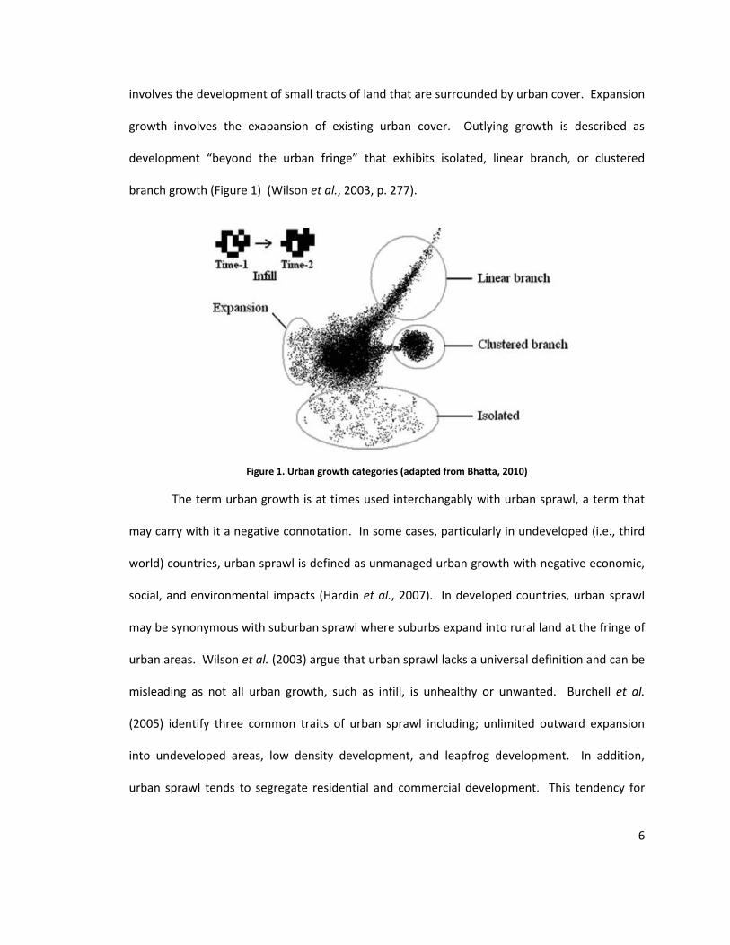
14). Three classes of urban growth include infill, expansion, and outlying growth. Infill growth
6
involves the development of small tracts of land that are surrounded by urban cover. Expansion
growth involves the exapansion of existing urban cover. Outlying growth is described as
development “beyond the urban fringe” that exhibits isolated, linear branch, or clustered
branch growth (Figure 1) (Wilson et al., 2003, p. 277).
Figure 1. Urban growth categories (adapted from Bhatta, 2010)
The term urban growth is at times used interchangably with urban sprawl, a term that
may carry with it a negative connotation. In some cases, particularly in undeveloped (i.e., third
world) countries, urban sprawl is defined as unmanaged urban growth with negative economic,
social, and environmental impacts (Hardin et al., 2007). In developed countries, urban sprawl
may be synonymous with suburban sprawl where suburbs expand into rural land at the fringe of
urban areas. Wilson et al. (2003) argue that urban sprawl lacks a universal definition and can be
misleading as not all urban growth, such as infill, is unhealthy or unwanted. Burchell et al.
(2005) identify three common traits of urban sprawl including; unlimited outward expansion
into undeveloped areas, low density development, and leapfrog development. In addition,
urban sprawl tends to segregate residential and commercial development. This tendency for
7
less mixed use land-use can be attributed to standardized and predictable (i.e., less risky) types
of development, automobile dependence, and a lack of regional authoritative land-use planning
(Burchell et al., 2005).
An in-depth review of the causes and effects of sprawl is beyond the scope of this study,
but the crux of the problem is that land development outpaces infrastructure. Rapid
development beyond the urban fringe can overwhelm local governments’ ability to provide
services such as basic utilities, transportation, and housing infrastructure (Hardin et al., 2007).
Additional public services such as police, fire protection, and education add to the burden of
government as well as cost to tax payers. Burchell et al. (2005, p. 6) argue that in the United
States cost is the primary concern of sprawl, as “the majority of the American public is not
unhappy with current pattern of development in metropolitan areas.” By virtue of its existence
sprawl does provide benefits which are hard to ignore such as reduced housing cost, increased
home ownership, increased home and lot size, lower crime rates, greater school choice, and
greater consumer choice (Burchell et al., 2005). So the question is not whether urban growth
will occur, but rather how has it grown, how will it grow, and ultimately how much will it cost?
Studies such as this research that seek to find optimal ways to map, measure, and quantify
urban growth can enhance our understanding of this phenomenon to help answer these
questions.
Using Census Data to Measure Urban Growth
The ability to measure urban growth directly from census data is highly limited due to
the aforementioned MAUP and broad census urban area designations. Measuring population
change and population density change may be a useful proxy for measuring urban growth
though. Census enumeration units (e.g. blocks, block groups, tracts) can be analyzed across
8
census years to calculate population change, population density change, and growth rate. A
problem that invariably arises is the change of enumeration unit boundaries from one census to
the next due to splitting, merging, or boundary adjustments. To account for these boundary
changes, the U.S. Census Bureau provides relationship files that allow for population
comparisons between census years.
Taking a 2010 census tract relationship file for example, each record in the relationship
file represents a polygon that is formed when the 2010 census tracts overlay the 2000 tracts.
Relationships may include no change between censuses, boundary revisions, the merging of
several tracts, or the splitting of a tract. Once relationships are established, population statistics
from 2010 census tracts may be assigned to 2000 tracts and change statistics may be calculated.
Population change and population density change statistics per enumeration unit may
be performed by simple subtraction. The growth rate may also be calculated and is defined as
the percent change between successive censuses and is expressed simply as:
Equation 1 (Parker, 2002)
Where: = Percent growth rate = Present or more recent population = Past population
In addition, population projections, and subsequent change statistics, may easily be
performed in a GIS using a table calculator or in a spreadsheet software program such as
Microsoft Excel. Thematic mapping of these change statistics in a GIS can highlight census units
that have experienced large population increase, high growth rates, and population density
changes. These maps can be useful, albeit limited, indicators of urban growth.
9
Using Satellite Remote Sensing Data to Measure Urban Growth
Although satellite sensor systems are generally lower in spatial and spectral resolution
compared to airborne imaging and hyperspectral technology, they are well suited for regional
urban analysis as they are more stable and cost effective, with high revisit rates and a wealth of
archived data. In addition, satellite images provide complete regional coverage without the
problem of imagery stopping at political boundaries (Wilson et al., 2003). de Paul (2007, p.
2267) states that with advances in technology, satellite sensors have “found more applications
in the analysis and planning of urban environments,” and “are producing data with high
potential for use in scientific and technological investigations.” Landsat in particular has been
invaluable for its longevity and resulting image library. Campbell (2007, p. 180), states that over
the last 30 years, Landsats 1 through 7 (excluding Landsat 6 which was lost at launch) have
maintained “consistent spectral definitions, resolutions, and scene characteristics, while taking
advantage of improved technology, calibration, and efficiency of data transmission.” This data
collection consistency is vital to monitoring long-term land-cover changes in studies such as this
that span decades.
Over 30 years of Landsat imagery archives provide a unique resource for analyzing and
measuring urban growth. Essential to this analysis is the ability to detect urban land-cover
change over the span of years and even decades. The most common approach to assess urban
growth is to classify and detect change from natural-cover to impermeable surfaces such as
rooftops, roads, and parking lots, as these “have been proven to be key indicators for identifying
the spatial extent and intensity of urbanization and urban sprawl” (Xian and Crane, 2005, p.204).
Urban areas are inherently difficult to classify though, due to the variety of spectral signatures
(i.e., surface reflectance) in urban environments. The mixed pixel problem exists due to the high
10
heterogeneity per pixel that exists in most urban scenes. This is a significant problem when
classifying imagery from medium to low resolution satellite remote sensors such as Landsat (i.e.,
30 meter resolution). In urban environments in particular, the spectral signature of a pixel may
be a composite of several land-cover classes such as vegetation and asphalt. Spectral confusion
can also make urban classification difficult due to reflectance similarites among land-covers such
as 1) water, dark impervious surfaces, and shadows, 2) dry soil, commercial / industrial land, and
dense residential land, and 3) forests and low density residential land (Lu and Weng, 2006). One
can conclude that there are unavoidable trade-offs between the high temporal resolution and
platform stability of satellite remote sensors and the high spectral and spatial resolution of
airborne systems.
Taking the aforementioned caveats into consideration, urban growth can readily be
measured from satellite derived classified images by performing change detection. Jensen and
Im (2007) outline the required steps involved in most, if not all, change detection studies. These
include, 1) specify the nature of the change detection problem, 2) identify environmental
considerations and select the remote sensing system to be used, 3) process data by applying
change detection techniques, and 4) evaluate the results. The two primary types of change
detection are image based (i.e., image-to-image) and classification based (i.e., map-to-map)
(Xian and Crane, 2005). The most commonly used change detection methods include image
overlay, post-classification comparison, spectral-temporal classification, image differencing,
image ratioing, image regression, and principal component analysis. Additional innovative
methods include change vector analysis, artificial neural networks, decision trees, and intensity-
hue-saturation transform (Hardin et al., 2007).
11
Dasymetric Mapping
Dasymetric mapping displays areas of homogeneity in data and is based on the idea that
mapped areas “will have small internal magnitude variations, while there will be larger
magnitude variations between mapped areas” (Kimerling et al., 2009, p. 163). More over, the
extent of populated areas serve as the denominator for dasymetric population density
computations (Holt et al., 2004). The redistribution of population from source zones (i.e.,
census boundaries) to target zones (i.e., populated land-cover) is known as areal interpolation.
Areal interpolation functions are said to preserve the pycnophylactic property (i.e., volume
preserving) in that “no data is lost or created during the transformation” (Sleeter and Gould,
2007, p. 1; Tobler, 1979). Furthermore, all error is limited to variations within each original areal
unit (e.g. census block, block group, tract) since population is preserved through the
transformation (Mennis, 2003). Sleeter and Gould (2007) argue that even though the nature of
a population distribution is more realistically represented through dasymetric mapping, its
complexity and ancillary data requirements often deter cartographers from using this technique.
The simplest form of dasymetric mapping is the binary “populated” or “unpopulated”
approach where population totals are uniformly reassigned to populated areas. The primary
advantage of this technique is that features such as lakes, rivers, agriculture, and uninhabited
lands are excluded from the interpolation providing a more accurate representation of
populatation distribution. An advanced form of the binary techniqe is the multi-class weighted
dasymetric techique (Ming-Dawa et al., 2010). This technique is based on the knowledge that
populated areas consist of unique areas with different population densities such as multi-family
developments versus single family neighborhoods. Weighting factors are assigned to each class
according to its characteristic population density. Additional information is required for this
12
technique that may include prior or expert knowledge, emperical sampling, or geo-statistical
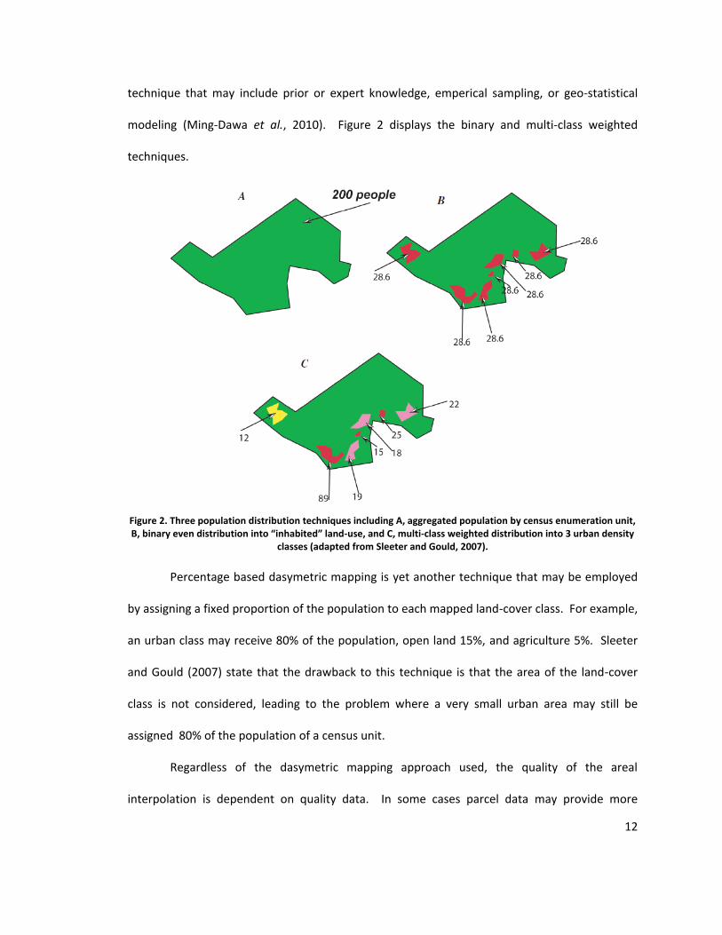
modeling (Ming-Dawa et al., 2010). Figure 2 displays the binary and multi-class weighted
techniques.
Figure 2. Three population distribution techniques including A, aggregated population by census enumeration unit, B, binary even distribution into “inhabited” land-use, and C, multi-class weighted distribution into 3 urban density
classes (adapted from Sleeter and Gould, 2007).
Percentage based dasymetric mapping is yet another technique that may be employed
by assigning a fixed proportion of the population to each mapped land-cover class. For example,
an urban class may receive 80% of the population, open land 15%, and agriculture 5%. Sleeter
and Gould (2007) state that the drawback to this technique is that the area of the land-cover
class is not considered, leading to the problem where a very small urban area may still be
assigned 80% of the population of a census unit.
Regardless of the dasymetric mapping approach used, the quality of the areal
interpolation is dependent on quality data. In some cases parcel data may provide more
13
accurate and reliable land-use and land-cover data than is possible with remotely sensed
imagery. In addition to land-use attributes, parcel databases may provide information on
building types and density parameters that may be useful for population density classifications.
A study by Sleeter and Gould (2007) used parcel land-use attributes rather than remotely sensed
land-cover classification to define high density, medium density, low density, and uninhabited
density classes. A land-use/land-cover raster layer was created from the parcel data density
classes to successfully redistribute population for Clatsop County, Oregon. In studies where
parcel data is not availiable or historical data is required, the use of land-cover classification
from satellite imagery may be the next viable approach. In these cases, the quaility and
accuracy of the dasymetric map has a direct correlation with the quality and accuracy of the
land-cover classification (Sleeter and Gould, 2007).
A study by Mennis (2003) demonstrates the use of a remotely sensed urban land-cover
dataset to define categories of urbanization as high, low, and non-urban. The author suggests
that urbanization data derived from satellite imagery provides a “predictable positive
relationship between population density and the degree of urban development as indicated by
satellite imagery” (Mennis, 2003, p. 35). However, the author admits that with this approach
industrial areas that are highly urbanized and sparsely populated must be acknowleged as
anomolies that result in error. The author further states that although “satellite remote sensing
cannot indicate population density directly” it can describe the urban morphology of built-up
and nondeveloped areas, and as such, is a useful data source for dasymetric mapping (Mennis,
2003, p. 34). The approach that was taken for this study was to use land-cover classification
maps derived from satellite data to redistribute population to high, medium, and low density
classes using a multi-class weighted distribution technique.
14
Two factors must be considered when using a multi-class weighted distribution
technique. First, the relative difference in population densities among the three urban classes
must be determined. The DME performs an empirical sampling process that samples population
density values for each urban class. The sampling is performed by selecting all census tracts that
meet or exceed a “percent cover” declared by a user-defined threshold. The resulting value is
the population density fraction, indicating the percentage of a census tract’s total population
that should be assigned to a specific urban class within the census tract. The population density
fraction is expressed as:
Equation 2 (Mennis, 2003)
Where: = population density fraction of urban class , = population density of urban class , = population density of urban class (high), = population density of urban class (medium), and = population density of urban class (low)
The second factor to consider is the difference in census tract area occupied by each
urban class. The aforementioned population density fraction assumes that the census tracts are
equally divided in area by the three urban classes. In reality census tracts rarely, if ever, exhibit
an even spatial distribution of urban classes (i.e., 33.3% high, 33.3% medium, and 33.3% low).
The DME calculates the area ratio to adjust the population density fraction for each individual
census tract according to the difference in area occupied by each urban class. The area ratio of
a specific census tract can be found by dividing the area of the urban class within the census
tract by the total area of the census tract, and dividing this number by the expected percentage
(i.e., 33%) (Mennis, 2003). Area in this case is synonymous with number of raster grid cells. The
area ratio is expressed as:
15
Equation 3 (Mennis, 2003)
Where: = area ratio of urban class in census tract , = number of grid cells of urban class in census tract , and = number of grid cells in census tract
The DME combines the population density fraction and area ratio to compute the total
fraction. The total fraction indicates the amount of a census tract’s total population that should
be assigned to a specific urban class within that census tract. The total fraction is expressed as:
Equation 4 (Mennis, 2003)
Where: = total fraction of urban class in census tract , = population density fraction of urban class , = area ratio of urban class in census tract , = population density fraction of urban class (high), = population density fraction of urban class (medium), = population density fraction of urban class (low), = area ratio of urban class (high) in census tract , = area ratio of urban class (medium) in census tract , and = area ratio of urban class (low) in census tract
Census tract population is finally interpolated (i.e., assigned) to grid cells by equally
dividing population among the respective urban class grid cells within the census tract. The
“population assignment” to a grid cell within a census tract is expressed as:
Equation 5 (Mennis, 2003)
Where: = population assigned to one grid cell of urban class in census tract , = total fraction for urban class in census tract , = population of census tract , and = number of grid cells of urban class in census tract
16
Study Area
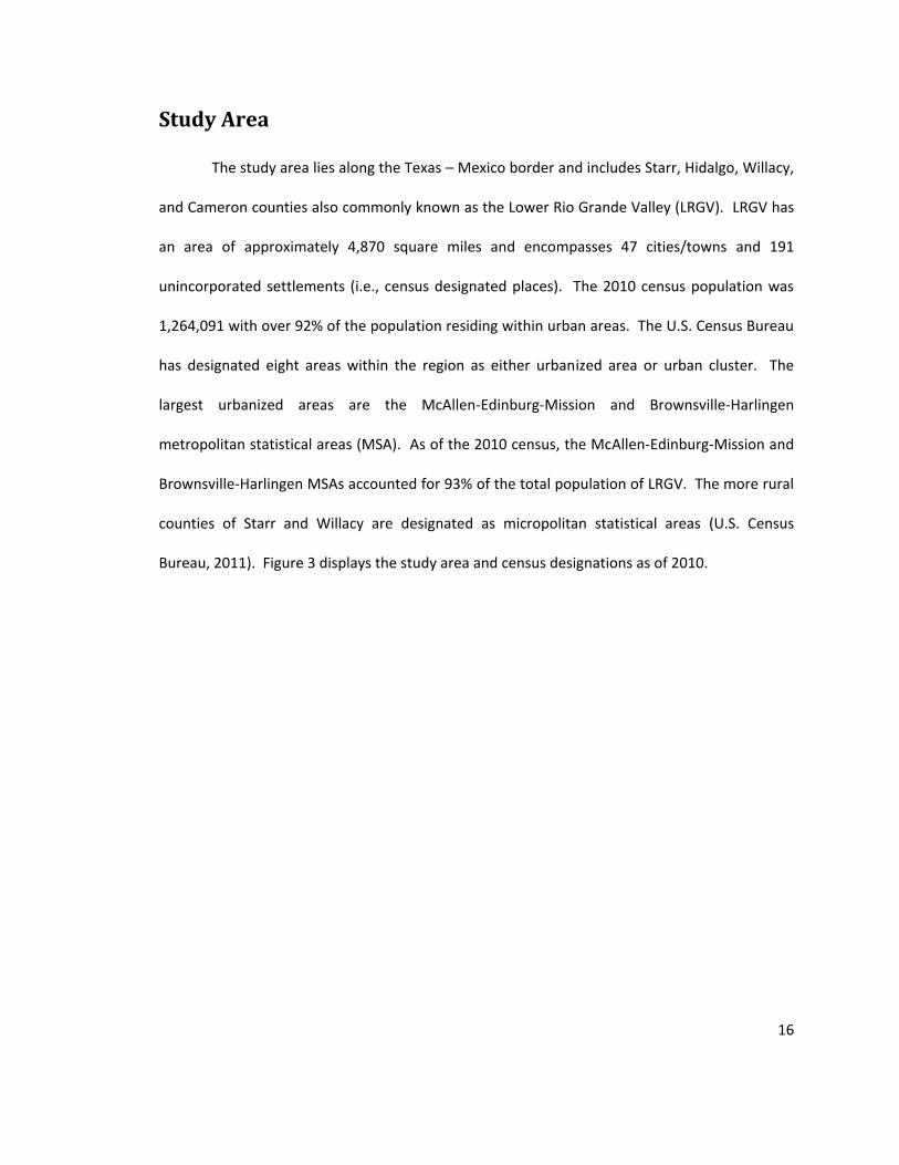
The study area lies along the Texas – Mexico border and includes Starr, Hidalgo, Willacy,
and Cameron counties also commonly known as the Lower Rio Grande Valley (LRGV). LRGV has
an area of approximately 4,870 square miles and encompasses 47 cities/towns and 191
unincorporated settlements (i.e., census designated places). The 2010 census population was
1,264,091 with over 92% of the population residing within urban areas. The U.S. Census Bureau
has designated eight areas within the region as either urbanized area or urban cluster. The
largest urbanized areas are the McAllen-Edinburg-Mission and Brownsville-Harlingen
metropolitan statistical areas (MSA). As of the 2010 census, the McAllen-Edinburg-Mission and
Brownsville-Harlingen MSAs accounted for 93% of the total population of LRGV. The more rural
counties of Starr and Willacy are designated as micropolitan statistical areas (U.S. Census
Bureau, 2011). Figure 3 displays the study area and census designations as of 2010.
17
Figure 3. LRGV counties, metropolitan and micropolitan statistical areas, and urban census designations (adapated
from U.S. Census Bureau, 2011).
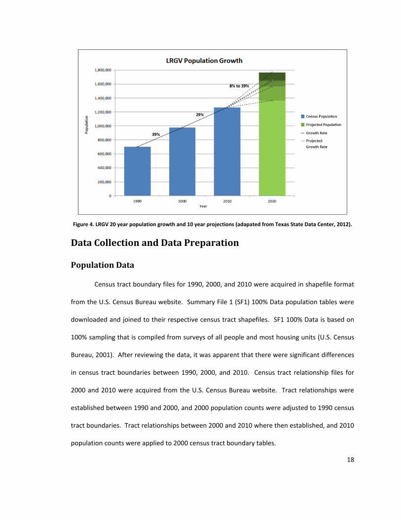
The LRGV region has experienced substantial growth over the last 20 years. From 1990
to 2000, the region witnessed a 39% growth rate, increasing in population by 276,494 people.
From 2000 to 2010 the growth rate was 29% with a population increase of 285,722 residents.
Conservative projections for 2020 project growth rates as low as 8%, while projections based on
historic migration rates project growth rates as high as 39% (Texas State Data Center, 2012)
(Figure 4). This amounts to possible increases in population ranging from nearly 100,000 to just
under 500,000 new residents over the next 10 years.
18
Figure 4. LRGV 20 year population growth and 10 year projections (adapated from Texas State Data Center, 2012).
Data Collection and Data Preparation
Population Data
Census tract boundary files for 1990, 2000, and 2010 were acquired in shapefile format
from the U.S. Census Bureau website. Summary File 1 (SF1) 100% Data population tables were
downloaded and joined to their respective census tract shapefiles. SF1 100% Data is based on
100% sampling that is compiled from surveys of all people and most housing units (U.S. Census
Bureau, 2001). After reviewing the data, it was apparent that there were significant differences
in census tract boundaries between 1990, 2000, and 2010. Census tract relationship files for
2000 and 2010 were acquired from the U.S. Census Bureau website. Tract relationships were
established between 1990 and 2000, and 2000 population counts were adjusted to 1990 census
tract boundaries. Tract relationships between 2000 and 2010 where then established, and 2010
population counts were applied to 2000 census tract boundary tables.
19
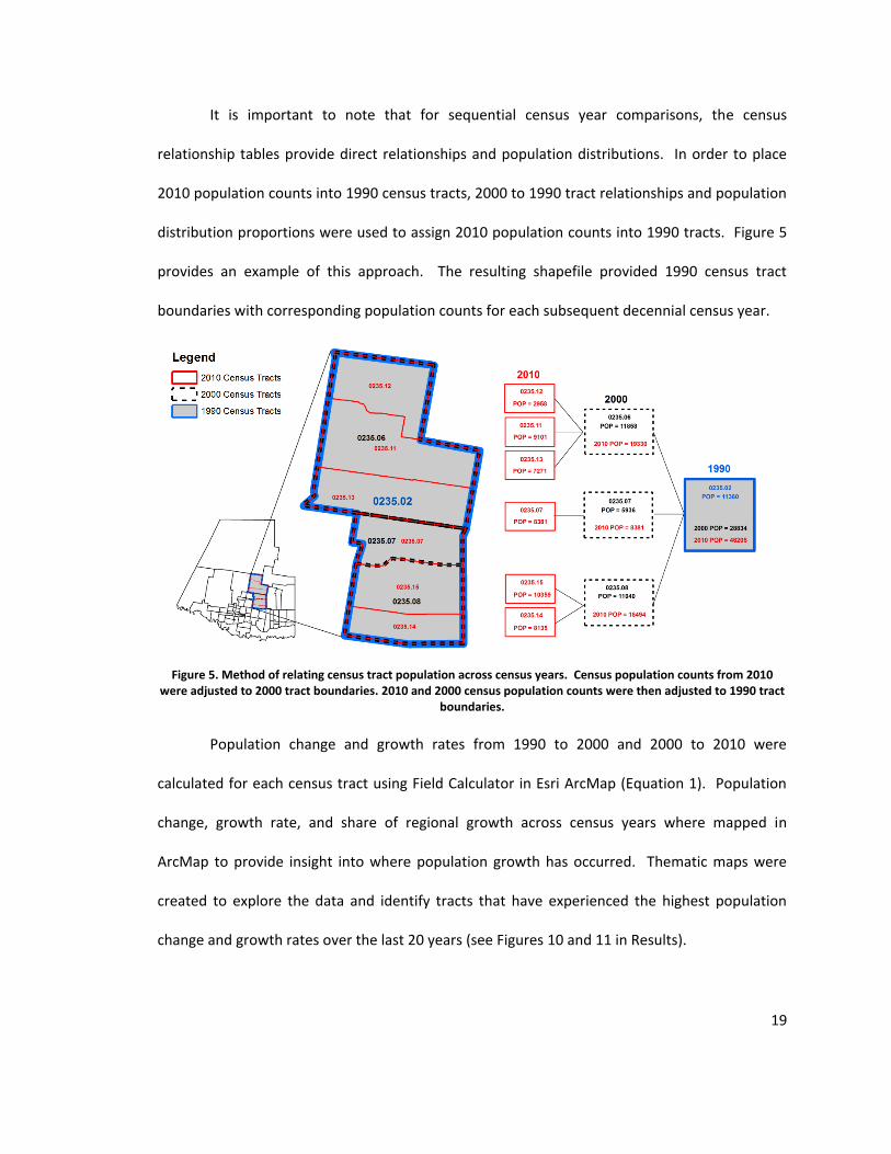
It is important to note that for sequential census year comparisons, the census
relationship tables provide direct relationships and population distributions. In order to place
2010 population counts into 1990 census tracts, 2000 to 1990 tract relationships and population
distribution proportions were used to assign 2010 population counts into 1990 tracts. Figure 5
provides an example of this approach. The resulting shapefile provided 1990 census tract
boundaries with corresponding population counts for each subsequent decennial census year.
Figure 5. Method of relating census tract population across census years. Census population counts from 2010
were adjusted to 2000 tract boundaries. 2010 and 2000 census population counts were then adjusted to 1990 tract boundaries.
Population change and growth rates from 1990 to 2000 and 2000 to 2010 were
calculated for each census tract using Field Calculator in Esri ArcMap (Equation 1). Population
change, growth rate, and share of regional growth across census years where mapped in
ArcMap to provide insight into where population growth has occurred. Thematic maps were
created to explore the data and identify tracts that have experienced the highest population
change and growth rates over the last 20 years (see Figures 10 and 11 in Results).
20
Satellite Imagery
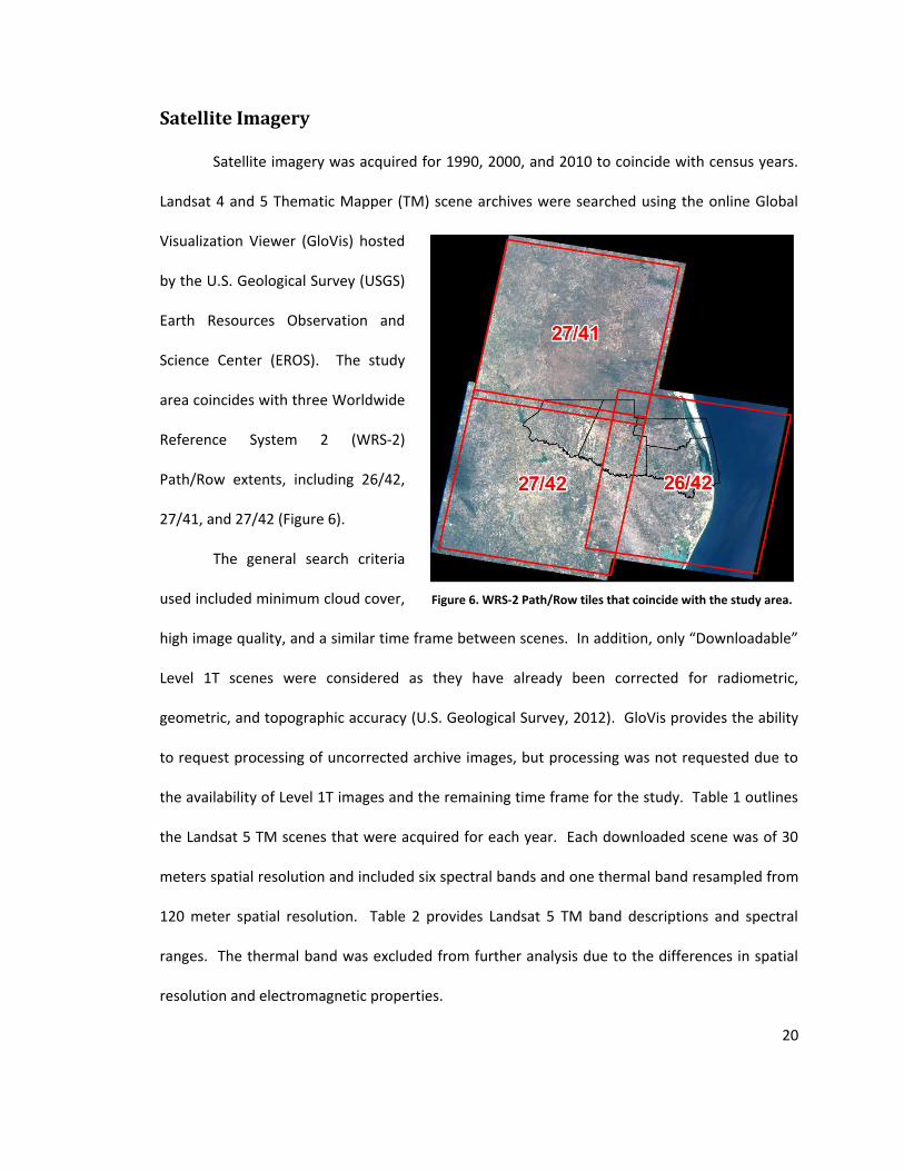
Satellite imagery was acquired for 1990, 2000, and 2010 to coincide with census years.
Landsat 4 and 5 Thematic Mapper (TM) scene archives were searched using the online Global
Visualization Viewer (GloVis) hosted
by the U.S. Geological Survey (USGS)
Earth Resources Observation and
Science Center (EROS). The study
area coincides with three Worldwide
Reference System 2 (WRS-2)
Path/Row extents, including 26/42,
27/41, and 27/42 (Figure 6).
The general search criteria
used included minimum cloud cover,
high image quality, and a similar time frame between scenes. In addition, only “Downloadable”
Level 1T scenes were considered as they have already been corrected for radiometric,
geometric, and topographic accuracy (U.S. Geological Survey, 2012). GloVis provides the ability
to request processing of uncorrected archive images, but processing was not requested due to
the availability of Level 1T images and the remaining time frame for the study. Table 1 outlines
the Landsat 5 TM scenes that were acquired for each year. Each downloaded scene was of 30
meters spatial resolution and included six spectral bands and one thermal band resampled from
120 meter spatial resolution. Table 2 provides Landsat 5 TM band descriptions and spectral
ranges. The thermal band was excluded from further analysis due to the differences in spatial
resolution and electromagnetic properties.
Figure 6. WRS-2 Path/Row tiles that coincide with the study area.
21
The existence of multiple scenes across the study area required that raster mosaics be
created for each band, for each year. The ArcMap Mosaic tool was used to merge multiple
scenes for each band using the default settings. The band mosaics where then stacked into
composite images using the Composite Bands tool. The resulting files included three 6-band
composite images for each year. The composite bands where then clipped to the LRGV study
area feature class. Three commonly used band combinations where created for each year,
including natural color (RGB=321), false color near-infrared (NIR) (RGB=432), and false color
short-wave infrared (SWIR) (RGB=742). Urban areas are typically displayed as white to light blue
in natural color composites, blue to grey in NIR composites, and lavender in SWIR composites
(NASA, 2012). The intention was to visually explore and evaluate the imagery in these
combinations to best differentiate urban areas of varying density.
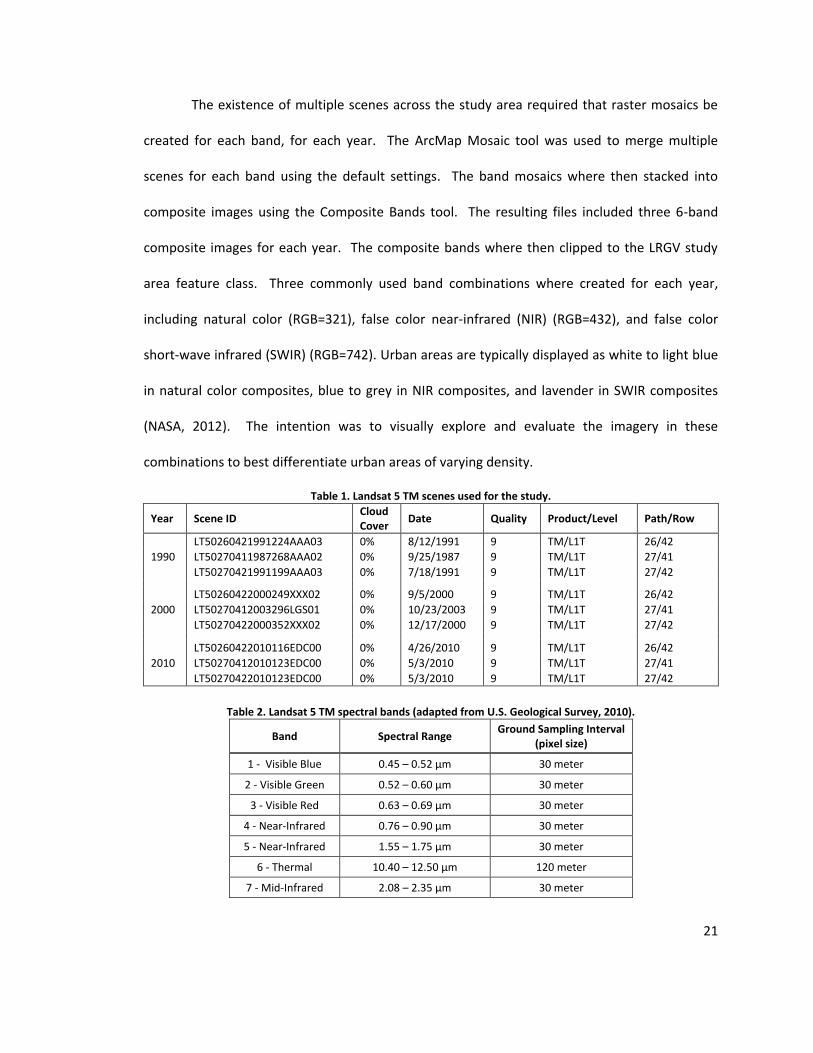
Table 1. Landsat 5 TM scenes used for the study.
Year Scene ID Cloud Cover
Date Quality Product/Level Path/Row
LT50260421991224AAA03 0% 8/12/1991 9 TM/L1T 26/42
1990 LT50270411987268AAA02 0% 9/25/1987 9 TM/L1T 27/41
LT50270421991199AAA03 0% 7/18/1991 9 TM/L1T 27/42
LT50260422000249XXX02 0% 9/5/2000 9 TM/L1T 26/42
2000 LT50270412003296LGS01 0% 10/23/2003 9 TM/L1T 27/41
LT50270422000352XXX02 0% 12/17/2000 9 TM/L1T 27/42
LT50260422010116EDC00 0% 4/26/2010 9 TM/L1T 26/42
2010 LT50270412010123EDC00 0% 5/3/2010 9 TM/L1T 27/41
LT50270422010123EDC00 0% 5/3/2010 9 TM/L1T 27/42
Table 2. Landsat 5 TM spectral bands (adapted from U.S. Geological Survey, 2010).
Band Spectral Range Ground Sampling Interval
(pixel size)
1 - Visible Blue 0.45 – 0.52 µm 30 meter
2 - Visible Green 0.52 – 0.60 µm 30 meter
3 - Visible Red 0.63 – 0.69 µm 30 meter
4 - Near-Infrared 0.76 – 0.90 µm 30 meter
5 - Near-Infrared 1.55 – 1.75 µm 30 meter
6 - Thermal 10.40 – 12.50 µm 120 meter
7 - Mid-Infrared 2.08 – 2.35 µm 30 meter
22
Methodology
Assumptions and Limitations
Assumptions and limitations inherent in this study must be noted in order to properly
assess the results. The choice to use census tracts as enumeration units was made to increase
the contrast between choropleth and dasymetric population density results, and to reduce the
amount of processing involved in establishing relationships across census years. It can be
argued that smaller census enumeration units such as block groups or blocks may reduce MAUP
effects and even reduce the need for dasymetric techniques in certain areas. This may be true
for densely built up areas, but census block groups and even blocks can be relatively large in
more rural areas that are generally not homogeneous. It is also important to note that
dasymetric population density results do not eliminate the MAUP effect, although they greatly
reduce it relative to the spatial resolution of the ancillary raster data used (i.e., 30 meter
resolution in the case of this study).
Census tract relationships were established in order to compare population change from
one decennial census to the next. This was accomplished using census tract relationship files.
Relationship files relating 1990 to 2000 and 2000 to 2010 were available from the U.S. Census
Bureau website, but no relationship file was available to relate 2010 to 1990. In order to relate
2010 to 1990 it was assumed that population distribution proportions from 2010 to 1990 would
be the same as those that existed between 2000 and 1990. In other words, 2000 to 1990
relationships were used to carry over 2010 population counts into 1990 census boundaries. This
was required to compare multi-decade census population counts and dasymetric population
distributions.
23
The methodology used to produce the three-class urban raster classifications was
limited in that urban density classes were defined arbitrarily through visual interpretation and
personal knowledge of the study area. This approach, which may be described as “you know it
when you see it,” is not a consistent, reproducible method for urban land-cover classification.
The use of percent imperviousness to categorize urban density classes would be much more
useful in a study such as this, although this approach was not taken largely due time constraints.
Additionally, at the outset of the study it was decided that urban areas would be inclusive of
residential, commercial, industrial, and transportation land-covers. This is problematic,
particularly for high density urban areas that inevitably include commercial and industrial
development. Population was interpolated into these highly urbanized and sparsely populated
areas that must be acknowledged as anomolies that result in error (Mennis, 2003).
The classification method used is the maximum likelihood supervised classification
which requires a set of predefined spectral signatures, derived either from user defined training
samples or iteratively defined classes (i.e., clusters). One should ideally experiment with
different classifiers to assess the sensitivity of results to the classification method used. Due to
time constraints and limitations in user experience, maximum likelihood was chosen for its
straightforward application and well documented use. Additionally, a quantitative accuracy
assessment of the urban raster classifications would have benefited this study. Acquiring high
resolution reference imagery from 10 and 20 years ago that coincided directly with the Landsat
data proved to be difficult. Furthermore, in situ ground truthing was not feasible for this study
that spanned two decades. That said, attempts where made to thoroughly review and correct
classification errors that were identified through visual assessments.
24
Analysis
Urban Land-Cover Classification
A prerequisite to the multi-class dasymetric mapping technique used for this study was
the creation of a three-class raster representing high, medium, and low density urban land-
covers, as well as an uninhabited class. All classification tasks were performed in ArcMap using
the Spatial Analyst Image Classification toolbar. Following work done by Hammann (2012), a 30
class ISO Cluster unsupervised classification was run for each year to define a set of spectral
signatures for subsequent supervised classifications. The resulting unsupervised classifications
were evaluated to identify areas of rural land that may spectrally resemble urban land-covers.
In order to account for phenological factors that influence spectral signatures, training samples
and spectral signatures were created for each year. Google Earth’s time slider tool was used to
explore historic high-resolution imagery that coincided with census years to verify training
samples. Imagery was available as far back as 1995, and up to 2010. Using personal knowledge
of the study area and the historic imagery in Google Earth, training samples were collected
visually with a focus on capturing signatures for high, medium, and low urban density land-
covers. High density urban land-cover was defined as downtown areas and central
business/commercial districts. Medium density urban land-cover included residential areas (i.e.,
subdivisions) in close proximity to downtown areas and within their respective city limits. Low
density urban land-cover included residential development outside of city limits that generally
exhibited isolated development patterns. To maintain consistency, an attempt was made to
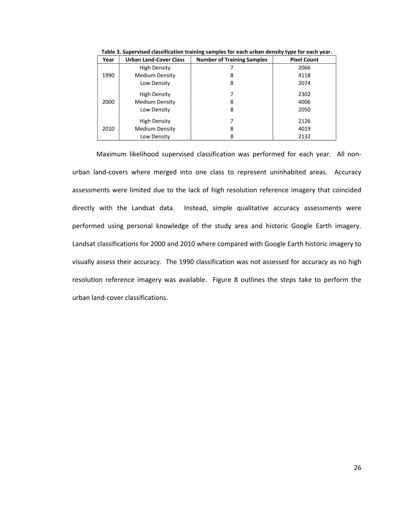
collect the same number of training samples and pixels for each urban density type. Table 3
identifies the number of training samples and pixels collected for each urban density type for
each year. Unsupervised classification rasters were also used to verify urban training samples as
25
well as to help identify uninhabited
land-covers that may be confused
for urban land-cover. Additional
training samples were collected to
identify uninhabited land-cover
signatures for agriculture, water,
natural areas, and cleared/vacant
land. Figure 7 demonstrates the
type of training samples that were
collected by land cover class using
visual cues and first-hand
knowledge. Color composite
images were used for training
sample collection as many surface
features are known to exhibit a
characteristic appearance based on
the spectral band combination
used. Signature files for each year
were created using the Create Signatures tool in the Image Classification toolbar.
Figure 7. Example of the type of training samples collected by land-cover type and color composite band combination.
26
Table 3. Supervised classification training samples for each urban density type for each year.
Year Urban Land-Cover Class Number of Training Samples Pixel Count
High Density 7 2066
1990 Medium Density 8 4118
Low Density 8 2074
High Density 7 2302
2000 Medium Density 8 4006
Low Density 8 2050
High Density 7 2126
2010 Medium Density 8 4019
Low Density 8 2132
Maximum likelihood supervised classification was performed for each year. All non-
urban land-covers where merged into one class to represent uninhabited areas. Accuracy
assessments were limited due to the lack of high resolution reference imagery that coincided
directly with the Landsat data. Instead, simple qualitative accuracy assessments were
performed using personal knowledge of the study area and historic Google Earth imagery.
Landsat classifications for 2000 and 2010 where compared with Google Earth historic imagery to
visually assess their accuracy. The 1990 classification was not assessed for accuracy as no high
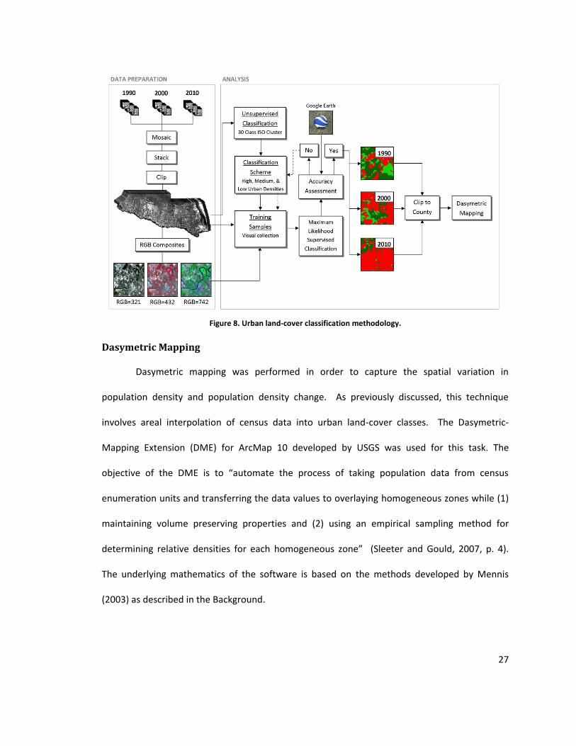
resolution reference imagery was available. Figure 8 outlines the steps take to perform the
urban land-cover classifications.
27
Figure 8. Urban land-cover classification methodology.
Dasymetric Mapping
Dasymetric mapping was performed in order to capture the spatial variation in
population density and population density change. As previously discussed, this technique
involves areal interpolation of census data into urban land-cover classes. The Dasymetric-
Mapping Extension (DME) for ArcMap 10 developed by USGS was used for this task. The
objective of the DME is to “automate the process of taking population data from census
enumeration units and transferring the data values to overlaying homogeneous zones while (1)
maintaining volume preserving properties and (2) using an empirical sampling method for
determining relative densities for each homogeneous zone” (Sleeter and Gould, 2007, p. 4).
The underlying mathematics of the software is based on the methods developed by Mennis
(2003) as described in the Background.
28
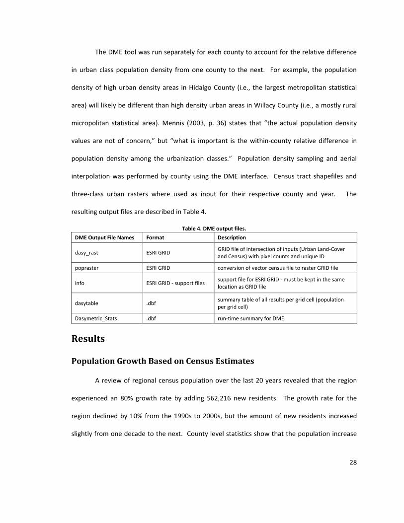
The DME tool was run separately for each county to account for the relative difference
in urban class population density from one county to the next. For example, the population
density of high urban density areas in Hidalgo County (i.e., the largest metropolitan statistical
area) will likely be different than high density urban areas in Willacy County (i.e., a mostly rural
micropolitan statistical area). Mennis (2003, p. 36) states that “the actual population density
values are not of concern,” but “what is important is the within-county relative difference in
population density among the urbanization classes.” Population density sampling and aerial
interpolation was performed by county using the DME interface. Census tract shapefiles and
three-class urban rasters where used as input for their respective county and year. The
resulting output files are described in Table 4.
Table 4. DME output files.
DME Output File Names Format Description
dasy_rast ESRI GRID GRID file of intersection of inputs (Urban Land-Cover and Census) with pixel counts and unique ID
popraster ESRI GRID conversion of vector census file to raster GRID file
info ESRI GRID - support files support file for ESRI GRID - must be kept in the same location as GRID file
dasytable .dbf summary table of all results per grid cell (population per grid cell)
Dasymetric_Stats .dbf run-time summary for DME
Results
Population Growth Based on Census Estimates
A review of regional census population over the last 20 years revealed that the region
experienced an 80% growth rate by adding 562,216 new residents. The growth rate for the
region declined by 10% from the 1990s to 2000s, but the amount of new residents increased
slightly from one decade to the next. County level statistics show that the population increase
29
in Hidalgo County drove much of this growth. Hidalgo County’s population doubled and
accounted for nearly 70% of the region’s growth. Cameron County provided a substantial share
of the growth with approximately 25%, while Starr and Willacy Counties combined for just under
5% of the growth for the region. All counties except for Hidalgo saw the majority of their
growth happen in the decade of the 1990s with a decline in growth rate and new residents
through the 2000 years. Like the region, the growth rate for Hidalgo County dropped from the
first decade to the second, but the number of new residents increased over the same time
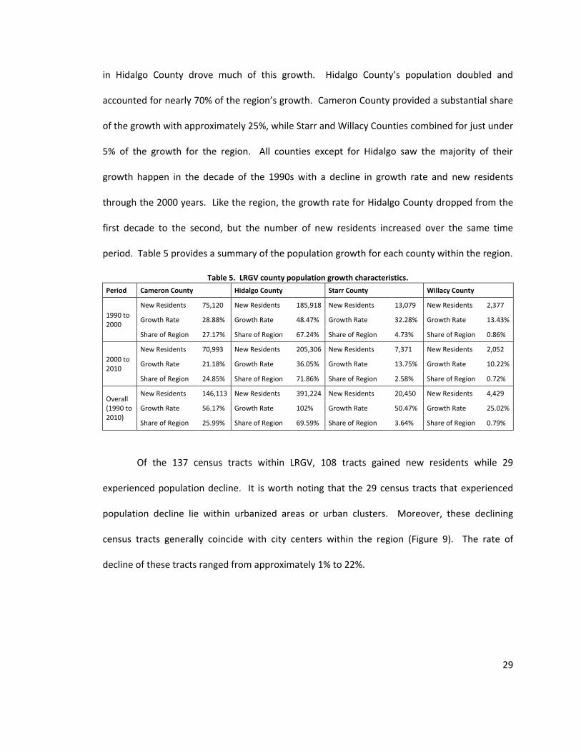
period. Table 5 provides a summary of the population growth for each county within the region.
Table 5. LRGV county population growth characteristics.
Period Cameron County Hidalgo County Starr County Willacy County
1990 to 2000
New Residents 75,120 New Residents 185,918 New Residents 13,079 New Residents 2,377
Growth Rate 28.88% Growth Rate 48.47% Growth Rate 32.28% Growth Rate 13.43%
Share of Region 27.17% Share of Region 67.24% Share of Region 4.73% Share of Region 0.86%
2000 to 2010
New Residents 70,993 New Residents 205,306 New Residents 7,371 New Residents 2,052
Growth Rate 21.18% Growth Rate 36.05% Growth Rate 13.75% Growth Rate 10.22%
Share of Region 24.85% Share of Region 71.86% Share of Region 2.58% Share of Region 0.72%
Overall (1990 to 2010)
New Residents 146,113 New Residents 391,224 New Residents 20,450 New Residents 4,429
Growth Rate 56.17% Growth Rate 102% Growth Rate 50.47% Growth Rate 25.02%
Share of Region 25.99% Share of Region 69.59% Share of Region 3.64% Share of Region 0.79%
Of the 137 census tracts within LRGV, 108 tracts gained new residents while 29
experienced population decline. It is worth noting that the 29 census tracts that experienced
population decline lie within urbanized areas or urban clusters. Moreover, these declining
census tracts generally coincide with city centers within the region (Figure 9). The rate of
decline of these tracts ranged from approximately 1% to 22%.

30
Figure 9. Census tracts with a negative growth rate from 1990 to 2010. Note that population counts were adjusted
to 1990 census boundaries.
The majority of the census tracts experienced population growth at varying rates from
1990 to 2000. 65 census tracts (approximately 47%) experienced a growth rate greater than
50%. 38 census tracts (approximately 28%) had population more than double in number with a
growth rate greater than 100%. A handful of census tracts experienced very high growth rates
with population growing three, four, and even five times over. These tracts lie exclusively in
Hidalgo and Cameron counties. Figure 10 displays the growth rate by census tract from 1990 to
2010.
31
Figure 10. Population growth rate by census tract from 1990 to 2010.
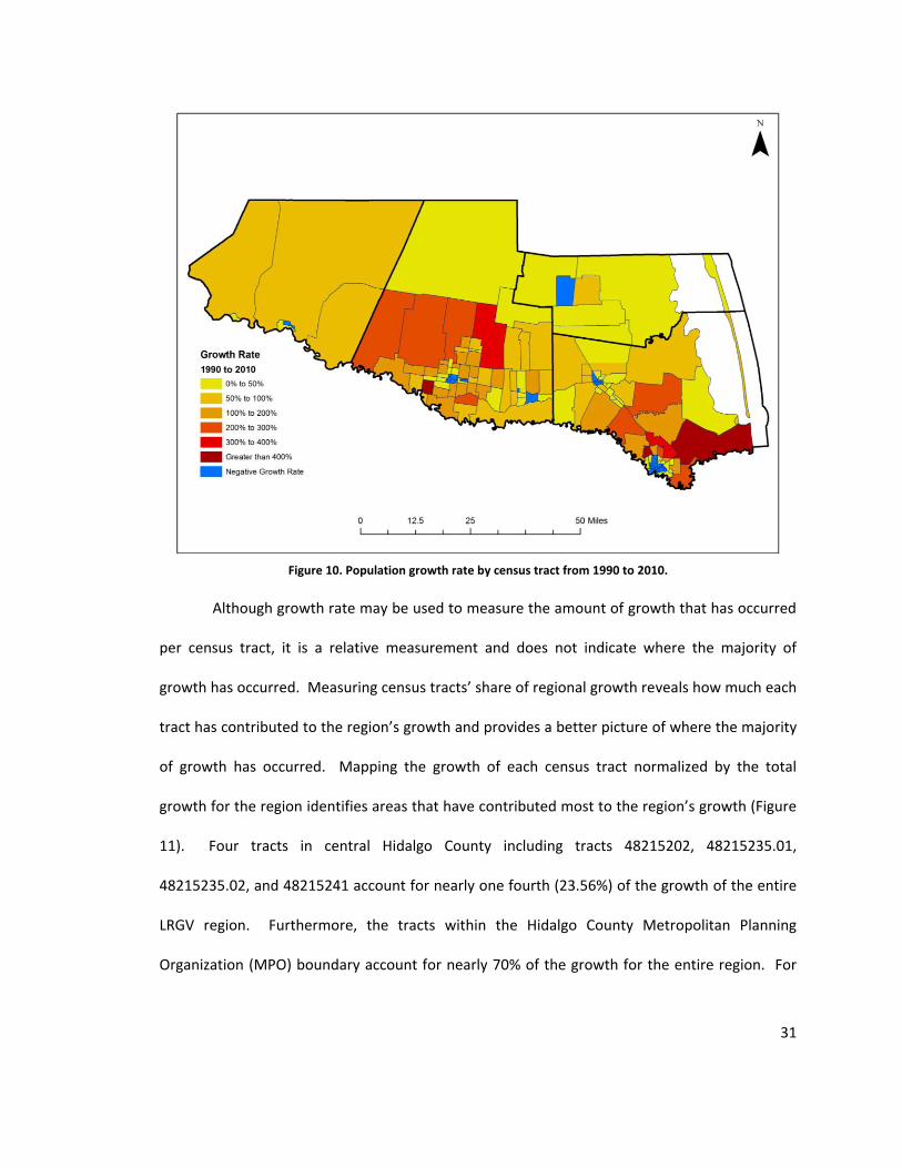
Although growth rate may be used to measure the amount of growth that has occurred
per census tract, it is a relative measurement and does not indicate where the majority of
growth has occurred. Measuring census tracts’ share of regional growth reveals how much each
tract has contributed to the region’s growth and provides a better picture of where the majority
of growth has occurred. Mapping the growth of each census tract normalized by the total
growth for the region identifies areas that have contributed most to the region’s growth (Figure
11). Four tracts in central Hidalgo County including tracts 48215202, 48215235.01,
48215235.02, and 48215241 account for nearly one fourth (23.56%) of the growth of the entire
LRGV region. Furthermore, the tracts within the Hidalgo County Metropolitan Planning
Organization (MPO) boundary account for nearly 70% of the growth for the entire region. For
32
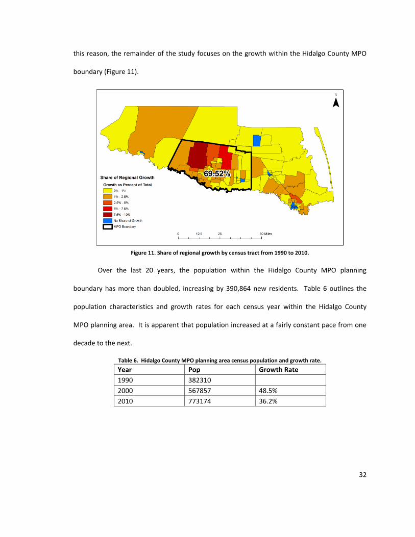
this reason, the remainder of the study focuses on the growth within the Hidalgo County MPO
boundary (Figure 11).
Figure 11. Share of regional growth by census tract from 1990 to 2010.
Over the last 20 years, the population within the Hidalgo County MPO planning
boundary has more than doubled, increasing by 390,864 new residents. Table 6 outlines the
population characteristics and growth rates for each census year within the Hidalgo County
MPO planning area. It is apparent that population increased at a fairly constant pace from one
decade to the next.
Table 6. Hidalgo County MPO planning area census population and growth rate.
Year Pop Growth Rate
1990 382310
2000 567857 48.5%
2010 773174 36.2%
33
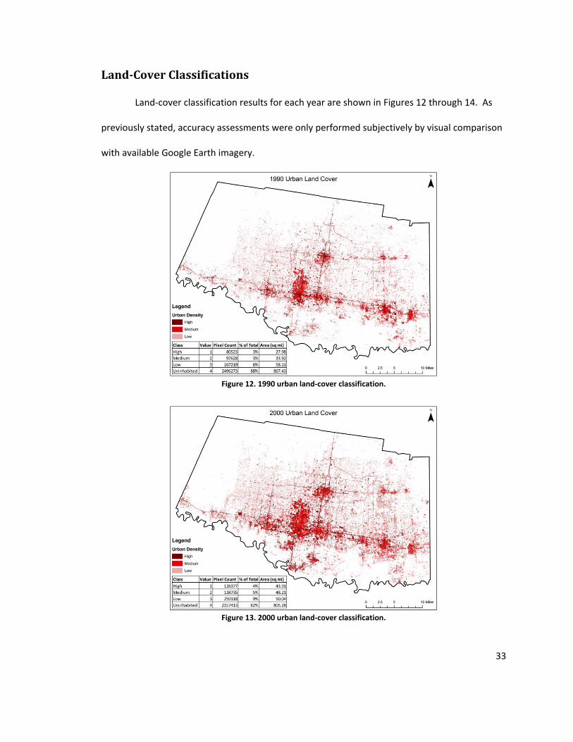
Land-Cover Classifications
Land-cover classification results for each year are shown in Figures 12 through 14. As
previously stated, accuracy assessments were only performed subjectively by visual comparison
with available Google Earth imagery.
Figure 12. 1990 urban land-cover classification.
Figure 13. 2000 urban land-cover classification.
34
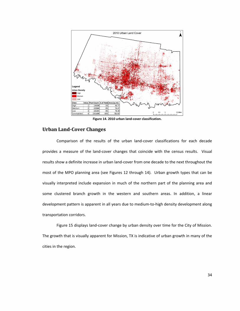
Figure 14. 2010 urban land-cover classification.
Urban Land-Cover Changes
Comparison of the results of the urban land-cover classifications for each decade
provides a measure of the land-cover changes that coincide with the census results. Visual
results show a definite increase in urban land-cover from one decade to the next throughout the
most of the MPO planning area (see Figures 12 through 14). Urban growth types that can be
visually interpreted include expansion in much of the northern part of the planning area and
some clustered branch growth in the western and southern areas. In addition, a linear
development pattern is apparent in all years due to medium-to-high density development along
transportation corridors.
Figure 15 displays land-cover change by urban density over time for the City of Mission.
The growth that is visually apparent for Mission, TX is indicative of urban growth in many of the
cities in the region.
35
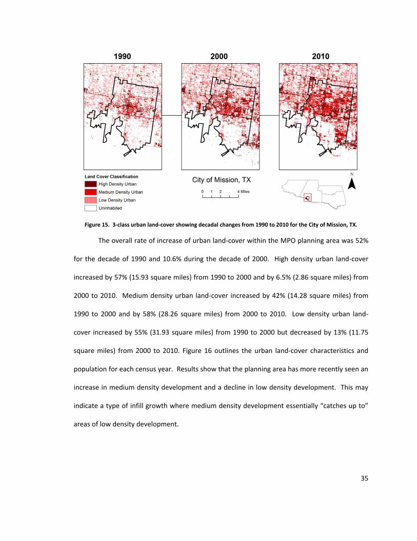
Figure 15. 3-class urban land-cover showing decadal changes from 1990 to 2010 for the City of Mission, TX.
The overall rate of increase of urban land-cover within the MPO planning area was 52%
for the decade of 1990 and 10.6% during the decade of 2000. High density urban land-cover
increased by 57% (15.93 square miles) from 1990 to 2000 and by 6.5% (2.86 square miles) from
2000 to 2010. Medium density urban land-cover increased by 42% (14.28 square miles) from
1990 to 2000 and by 58% (28.26 square miles) from 2000 to 2010. Low density urban land-
cover increased by 55% (31.93 square miles) from 1990 to 2000 but decreased by 13% (11.75
square miles) from 2000 to 2010. Figure 16 outlines the urban land-cover characteristics and
population for each census year. Results show that the planning area has more recently seen an
increase in medium density development and a decline in low density development. This may
indicate a type of infill growth where medium density development essentially “catches up to”
areas of low density development.
36
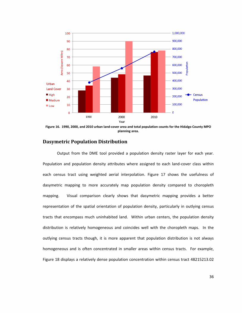
Figure 16. 1990, 2000, and 2010 urban land-cover area and total population counts for the Hidalgo County MPO
planning area.
Dasymetric Population Distribution
Output from the DME tool provided a population density raster layer for each year.
Population and population density attributes where assigned to each land-cover class within
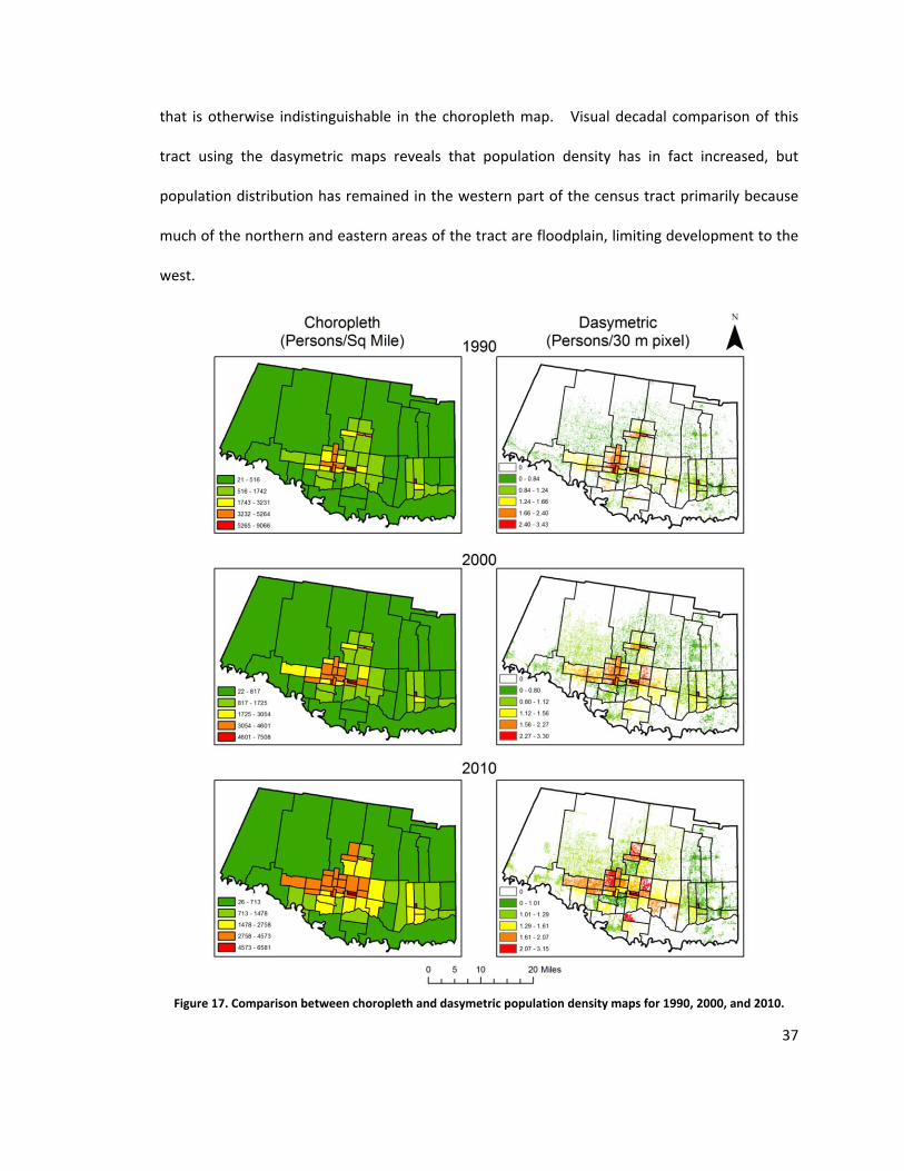
each census tract using weighted aerial interpolation. Figure 17 shows the usefulness of
dasymetric mapping to more accurately map population density compared to choropleth
mapping. Visual comparison clearly shows that dasymetric mapping provides a better
representation of the spatial orientation of population density, particularly in outlying census
tracts that encompass much uninhabited land. Within urban centers, the population density
distribution is relatively homogeneous and coincides well with the choropleth maps. In the
outlying census tracts though, it is more apparent that population distribution is not always
homogeneous and is often concentrated in smaller areas within census tracts. For example,
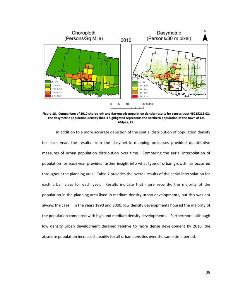
Figure 18 displays a relatively dense population concentration within census tract 48215213.02
37
that is otherwise indistinguishable in the choropleth map. Visual decadal comparison of this
tract using the dasymetric maps reveals that population density has in fact increased, but
population distribution has remained in the western part of the census tract primarily because
much of the northern and eastern areas of the tract are floodplain, limiting development to the
west.
Figure 17. Comparison between choropleth and dasymetric population density maps for 1990, 2000, and 2010.
38
Figure 18. Comparison of 2010 choropleth and dasymetric population density results for census tract 48215213.02.
The dasymetric population density that is highlighted represents the northern population of the town of Las Milpas, TX.
In addition to a more accurate depiction of the spatial distribution of population density
for each year, the results from the dasymetric mapping processes provided quantitative
measures of urban population distribution over time. Comparing the aerial interpolation of
population for each year provides further insight into what type of urban growth has occurred
throughout the planning area. Table 7 provides the overall results of the aerial interpolation for
each urban class for each year. Results indicate that more recently, the majority of the
population in the planning area lived in medium density urban developments, but this was not
always the case. In the years 1990 and 2000, low density developments housed the majority of
the population compared with high and medium density developments. Furthermore, although
low density urban development declined relative to more dense development by 2010, the
absolute population increased steadily for all urban densities over the same time period.
39
Table 7. Dasymetic population distribution totals for each urban land-cover type for 1990, 2000, and 2010.
Year High Density Medium Density Low Density Total
1990 102,027 (26.9%) 126,100 (33.2%) 151,183 (39.9%) 379,310
2000 155,622 (27.4%) 182,383 (32.1%) 229,852 (40.5%) 567,857
2010 197,735(25.6%) 303,921 (39.3%) 271,518 (35.1%) 773,174
Additionally, dasymetric results were evaluated for the four census tracts in central
Hidalgo County that contributed to nearly one fourth (23.56%) of the growth of the entire LRGV
region. Within the Hidalgo County MPO planning area, census tracts 48215202, 48215235.01,
48215235.02, and 48215241 accounted for 33.9% of the total population growth over the last
20 years. Comparing dasymetric results for each census tract, at each census year, revealed the
urban growth and population change that has occurred within each of these census tracts.
Figures 19 through 22 show the urban population growth characteristics for each of the
aforementioned census tracts. Results indicate that census tracts 48215202 and 48215235.01
have seen a marked increase in medium density population over the last 10 years. Census tracts
48215235.01, 48215235.02, and 48215241 have seen a constant rise in low density population
growth over the last 20 years. Census tract 48215202, which is smallest in area and closest to
the urban core, has seen a drop in low density urban development and a marked increase in
medium density development over the last 10 years. Overall, results indicate that although the
majority of the population now resides in medium density developments (Table 7), those areas
that are contributing most to population growth are still composed largely of low density urban
development.
40
Figure 19. Census tract 48215202 urban population distribution by year. Population growth rates were 68.9% and
27.9% from 1990 to 2000 and 2000 to 2010 respectively.
Figure 20. Census tract 48215235.01 urban population distribution by year. Population growth rates were 142.3%
and 56.4% from 1990 to 2000 and 2000 to 2010 respectively.
Figure 21. Census tract 48215235.02 urban population distribution by year. Population growth rates were 153.8%
and 60.2% from 1990 to 2000 and 2000 to 2010 respectively.

41
Figure 22. Census tract 48215241 urban population distribution by year. Population growth rates were 143.2% and
45.8% from 1990 to 2000 and 2000 to 2010 respectively.
Discussion and Conclusions
Summary of the Work
This study has demonstrated the utility of census data, satellite remote sensing data,
and dasymetric mapping techniques for measuring urban growth. Decennial censuses provide
aggregated population counts within enumeration units that can be spatially related across
census years. Population statistics can easily be calculated and mapped using attribute table
calculations and thematic mapping functions found in most GIS software packages. Satellite
platforms such as Landsat provide a wealth of imagery archives dating back more than 30 years.
Urban land-cover classifications that coincide with censuses can be used to provide quantitative
measures of change in the built environment. Furthermore, changes in multi-class urban land-
cover classifications provide insight into what type of urban growth has occurred. Dasymetric
mapping provides a method of combining census data and urban land-cover data to more
accurately map population density through aerial interpolation. Comparison of dasymetric
population density maps across census years provides a more accurate view than choropleth
maps of population density change. In addition, population distributions per enumeration unit
42
can be viewed to understand urban growth in those areas that have experienced the highest
population growth rates and contributed most to the region’s growth.
Future Work
This study only looked at a subset of the population and urban land-cover within the
study area. Future work should expand to the entire study area, looking at regional population,
urban land-cover changes, and individual census tract population distributions over time. The
methodology outlined in this study may also be used measure urban growth within specific city
boundaries and extraterritorial jurisdictions (ETJ) which may aid in local planning initiatives.
Additional measures that may indicate sprawl should also be explored. This may include
identifying tracts where low density land-cover has outpaced population growth, or where a
decline in high and medium density population coincides with a rise in low density population.
Further research is needed to understand how dasymetric results may be used to indicate urban
sprawl.
Population and land-cover projections may also be used as dasymetric inputs to project
population density and population distributions for future dates. Population projections can be
calculated using methods ranging from simple extrapolation to the cohort component technique
used by the U.S. Census Bureau. Results from land-use/land-cover change models may be used
in conjunction with these population projections to predict future population density and urban
population distribution. This would arguably be the most useful information for planners by
providing simulations of future urban growth that would influence present day planning
initiatives.
43
Bibliography
Bhatta, B. (2010). Advances in Geographic Information Science: Analysis of Urban Growth and
Sprawl from Remote Sensing Data. New York, NY: Springer.
Burchell, R. W., Downs, A., McCann, B., & Mukherji, S. (2005). Sprawl Costs: Economic Impacts of
Unchecked Development. Washington, DC: Island Press.
Campbell, J. B. (2007). Introduction to Remote Sensing (Fourth ed.). New York: The Guilford
Press.
de Paul, O. V. (2007). Remote Sensing: New Applications for Urban Areas. Proceedings of the
IEEE, 95(12), 2267-2268.
Hammann, G. M. (2012). Urban Growth Analysis Via Landsat. SatMagazine, 4(11), 44-53.
Hardin, P. J., Jackson, M. W., & Otterstrom, S. M. (2007). Mapping, Measuring, and Modeling
Urban Growth. In R. R. Jensen, J. D. Gatrell, & D. McLean, Geo-Spatial Technologies in
Urban Environments: Policy, Practice, and Pixels (pp. 141-176). Berlin: Springer.
Holt, J. B., Lo, C., & Hodler, T. W. (2004). Dasymetric Estimation of Population Density and Areal
Interpolation of Census Data. Cartography and Geographic Information Science, 31(2),
103-121.
Jensen, J. R., & Im, J. (2007). Remote Sensing Change Detection in Urban Environments. In R. R.
Jensen, J. D. Gatrell, & D. McLean, Geo-Spatial Technologies in Urban Environments:
Policy, Practice, and Pixels (pp. 7-31). Berlin: Springer.
Kimerling, J. A., Buckley, A. R., Muehrcke, P. C., & Muehrcke, J. O. (2009). Map Use: Reading and
Analysis (Sixth Edition ed.). Redlands, California: ESRI Press Academic.
44
Lu, D., & Weng, Q. (2006). Use of impervious surface in urban land-use classification. Remote
Sensing of Environment, 102(1-2), 146-160.
Mennis, J. (2003). Generating Surface Models of Population Using Dasymetric Mapping. The
Professional Geographer, 55(1), 31-42.
Ming-Dawa, S., Mei-Chun, L., Hsin-I, H., Bor-Wen, T., & Chun-Hung, L. (2010). Multi-layer multi-
class dasymetric mapping to estimate population distribution. Science of the Total
Environment, 408, 4807-4816.
NASA. (2012). An Introductory Landsat Tutorial. Retrieved September 5, 2012, from NASA -
Stennis Space Center: http://zulu.ssc.nasa.gov/mrsid/tutorial/Landsat%20Tutorial-
V1.html
Office of Management and Budget. (2010). 2010 Standards for Delineating Metropolitan and
Micropolitan Statistical Areas. Federal Register, 75(123), 37245-37252.
Parker, B. (2002, September 30). Calculating Growth Rates. Retrieved September 5, 2012, from
PPPM 613: Planning Analysis: http://pages.uoregon.edu/rgp/PPPM613/class8a.htm
Sleeter, R., & Gould, M. (2007). Geographic Information System Software to Remodel Population
Data Using Dasymetric Mapping Methods. Reston, Virginia: U.S. Geological Survey.
Smith, S. K., & Shahidullah, M. (1995). An Evaluation of Population Projection Errors for Census
Tracts. Journal of the American Statistical Association, 90(429), 64-71.
Texas State Data Center. (2012). Population Projections. Retrieved April 3, 2012, from Texas
State Data Center: http://idserportal.utsa.edu/sdc/projections/
Tobler, W. R. (1979). Smooth Pycnophylactic Interpolation for Geographical Regions. Journal of
the American Statistical Association, 74(367), 519-530.
45
U.S. Census Bureau. (2001). Census 2000 Summary File 1 Technical Documentation. United
States: U.S. Census Bureau.
U.S. Census Bureau. (2011, September 2). 2010 Census Urban and Rural Classification and Urban
Area Criteria. Retrieved December 8, 2011, from U.S. Census Bureau:
http://www.census.gov/geo/www/ua/2010urbanruralclass.html
U.S. Census Bureau. (2011). American FactFinder. Retrieved March 23, 2012, from U.S. Census
Bureau: http://census.factfinder2.gov
U.S. Geological Survey. (2010). Landsat 5 History. Retrieved September 2, 2012, from USGS
Landsat Missions: http://landsat.usgs.gov/about_landsat5.php
U.S. Geological Survey. (2012). Landsat Product Definitions. Retrieved April 3, 2012, from USGS
Global Visualization Viewer:
edcsns17.cr.usgs.gov/helpdocs/landsat/product_descriptions.html
Vigness, D. M., & Odintz, M. (2011, November 01). RIO GRANDE VALLEY. Retrieved November
01, 2011, from Handbook of Texas Online:
http://www.tshaonline.org/handbook/online/articles/ryr01
Weeks, J. R., Larson, D., & Fugate, D. (2005). Patterns of Urban Land Use as Assessed by Satellite
Imagery: An Application to Cairo, Egypt. In B. Entwisle, & R. S. Rindfuss, Population, Land
Use, Environment: Research Directions (pp. 265-286). Washington DC: National Academy
Press.
Wilson, E. H., Hurd, J. D., Civco, D. L., Prisloe, M. P., & Arnold, C. (2003). Development of a
geospatial model to quantify, describe and map urban growth. Remote Sensing of
Environment, 86(3), 275-285.

46
Xian, G., & Crane, M. (2005). Assessments of urban growth in the Tampa Bay watershed using
remote sensing data. Remote Sensing of Environment, 97(2), 203-215.