1

Using column generation to solve parallelmachine scheduling and RCPS problems with

minimax objective functions

Han Hoogeveen

Joint work withMarjan van den Akker, Guido Diepen, and Jules van Kempen

June 4, 2008

2

Problem description (1)

We have m identical machines M1, . . . ,Mm:

I Each machine is continuously available from time zeroonwards

I Each machine can handle one job at a time

All machines together must process n jobs/tasks J1, . . . , Jn.Processing job Jj requires an uninterrupted period of length pj

(independent of the machine).

A schedule specifies for each job during which period it isexecuted.

We want to find a feasible schedule that minimizes some objectivefunction of minimax type.

3

Problem description (2)

There are n jobs J1, . . . , Jn with

I processing time pj (≥ 0);

I due date dj (can be negative);

I release date rj (≥ 0);

I deadline d̄j .

All data are assumed to be integral.

There can be precedence constraints of the form:

I Jj must start at least X time units after Ji;

I Jj must start exactly X time units after Ji;

I Jj must start at most X time units after Ji.

4

Representation

A given schedule σ is specified through a set of completion timesC1, . . . , Cn.

A schedule is feasible if and only if

I rj ≤ Cj − pj (there is no work done before the release date)

I Cj ≤ d̄j (there is no work done after the deadline)

I all precedence constraints are satisfied

I at most m jobs are processed at the same time.

Given the execution intervals a schedule is constructed by assigningthe jobs in order of starting time Cj − pj to any free machine.

Objective function: minimize maximum lateness Lmax

Lmax = maxj{Cj − dj}.

5

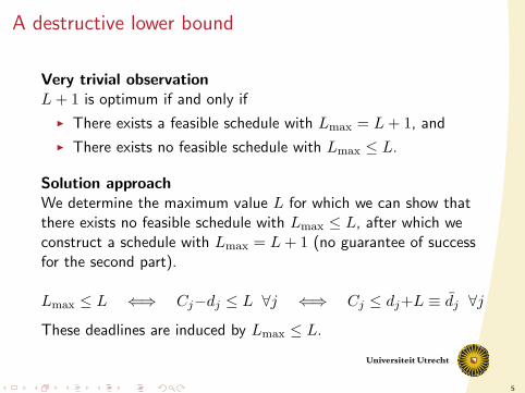
A destructive lower bound

Very trivial observationL + 1 is optimum if and only if

I There exists a feasible schedule with Lmax = L + 1, and

I There exists no feasible schedule with Lmax ≤ L.

Solution approachWe determine the maximum value L for which we can show thatthere exists no feasible schedule with Lmax ≤ L, after which weconstruct a schedule with Lmax = L + 1 (no guarantee of successfor the second part).

Lmax ≤ L ⇐⇒ Cj−dj ≤ L ∀j ⇐⇒ Cj ≤ dj+L ≡ d̄j ∀j

These deadlines are induced by Lmax ≤ L.

6

Useful observations

Any feasible schedule consists of m single-machine schedules thatall respect the induced deadlines, such that each job is part ofexactly one single-machine schedule.

The feasibility problem ‘does there exist a schedule withLmax ≤ L?’ is equivalent to the feasibility problem ‘Can you findm feasible, disjoint machine schedules that contain all jobs?’

Optimization variant: ‘minimize the number of feasible, disjointmachine schedules that you need to cover all jobs’.

The answer to the feasibility problem is ‘yes’ if and only if theoutcome value of the optimization problem is ≤ m.

7

Useful observations (2)

Instead of computing a ‘length-wise’ lower bound we compute alower bound on the number of single-machine schedules that areneeded =⇒ based on the width of the schedule.

Distinguishing between ≥ m + 1 and ≤ m gives a better gap withrespect to the percentage that the lower bound can be off.

8

P ||Lmax

Suppose the set S containing all feasible single-machine schedulesis known. Then the optimization problem is modelled as an ILP asfollows

I ajs = 1 if machine schedule s contains Jj and ajs = 0,otherwise

I Introduce a binary decision variable xs for each machineschedule s that gets the value 1 if s is selected

I We then get the following ILP-formulation:

minimize∑s∈S

xs

subject to ∑s∈S

ajsxs = 1, for each j = 1, . . . , n,

xs ∈ {0, 1}, for each s ∈ S.

9

Lower bound

Solve the LP-relaxation; if the outcome value is > m, then nofeasible schedule with Lmax ≤ L does exist.

Use column generation to solve the LP-relaxation to optimality.You then do not need to know all feasible single-machineschedules; you will generate only a subset of the single-machineschedules, containing all the ones you need.

10

LP-relaxation

minimize∑s∈S

xs

subject to ∑s∈S

ajsxs = 1, for each j = 1, . . . , n,

xs ≥ 0 for each s ∈ S.

Recall that

ajs ={

1 if Jj occurs in s0 otherwise

11

LP-theory

I The reduced cost of a feasible single-machine schedule s isequal to

c′s = cs −n∑

j=1

λjajs = 1−n∑

j=1

λjajs;

here λj is the known dual multiplier corresponding toconstraint j.

I The current subset of variables solves the original LP ifc′s ≥ 0 for all feasible single-machine schedules s ∈ S.

I Check optimality by solving the pricing problem: find thefeasible single-machine schedule s ∈ S with minimumreduced cost. If this is ≥ 0, then optimal; if < 0, then addthis variable and continue.

12

Elaboration for P ||Lmax

The pricing problem is equivalent to: find the feasiblesingle-machine schedule that maximizes

n∑j=1

λjajs.

Core problem: Include Jj in the single-machine schedule or not.Including Jj implies that it must be executed and completed bytime d̄j ; the reward is then λj =⇒ 1||

∑λjUj .

13

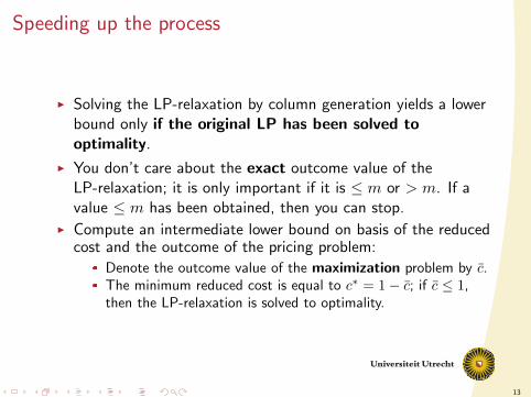
Speeding up the process

I Solving the LP-relaxation by column generation yields a lowerbound only if the original LP has been solved tooptimality.

I You don’t care about the exact outcome value of theLP-relaxation; it is only important if it is ≤ m or > m. If avalue ≤ m has been obtained, then you can stop.

I Compute an intermediate lower bound on basis of the reducedcost and the outcome of the pricing problem:

� Denote the outcome value of the maximization problem by c̄.� The minimum reduced cost is equal to c∗ = 1− c̄; if c̄ ≤ 1,

then the LP-relaxation is solved to optimality.

14

Intermediate lower bound (1)Since c∗ is the minimum reduced cost and cs = 1, we find

1 = cs = c′s +n∑

j=1

λjajs ≥ c∗ +n∑

j=1

λjajs

∑s∈S

xs ≥∑s∈S

(c∗ +n∑

j=1

λjajs)xs =

c∗∑s∈S

xs +∑s∈S

n∑j=1

λjajsxs =

c∗∑s∈S

xs +n∑

j=1

λj

[∑s∈S

ajsxs

]=

c∗∑s∈S

xs +n∑

j=1

λj

15

Intermediate lower bound (2)

Therefore, we find that

(1− c∗)∑s∈S

xs ≥n∑

j=1

λj

Since 1− c∗ = c̄ > 0, we find

∑s∈S

xs ≥n∑

j=1

λj/c̄

16

Optimal solution

Suppose that we have shown that Lmax ≤ L is impossible, but theoutcome value of the LP-relaxation for Lmax ≤ L + 1 is ≤ m.

We can solve the ILP by applying branch-and-bound using thebranching strategy by Van den Akker, Hoogeveen, Van de Veldefor P ||

∑wjCj (this is compatible with column generation).

17

Now P |rj|Lmax

I Same approach: translate the feasibility problem into anoptimization problem, formulate the ILP, and solve theLP-relaxation (a feasible machine schedule must obey therelease dates and induced deadlines).

I Complication: the maximization problem then becomes1|rj |

∑λjUj .

I Solution approach: do not solve the pricing problem tooptimality, but use local search to compute a near-optimalsolution.

I We can use the same intermediate lower bound as before. Wecompute the value of c̄ necessary to make the intermediatelower bound equal to m. Once-in-a-while, we check whetherthere exists a solution to the maximization problem with thisvalue or less. If it does not exist, then we know thatLmax ≤ L is not possible.

18

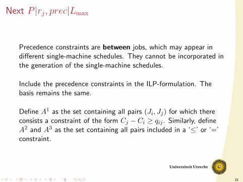
Next P |rj, prec|Lmax

Precedence constraints are between jobs, which may appear indifferent single-machine schedules. They cannot be incorporated inthe generation of the single-machine schedules.

Include the precedence constraints in the ILP-formulation. Thebasis remains the same.

Define A1 as the set containing all pairs (Ji, Jj) for which thereconsists a constraint of the form Cj − Ci ≥ qij . Similarly, defineA2 and A3 as the set containing all pairs included in a ‘≤’ or ‘=’constraint.

19

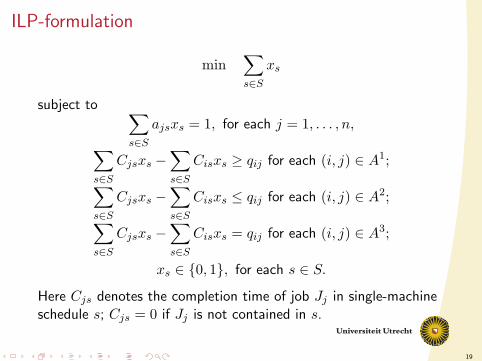
ILP-formulation

min∑s∈S

xs

subject to ∑s∈S

ajsxs = 1, for each j = 1, . . . , n,∑s∈S

Cjsxs −∑s∈S

Cisxs ≥ qij for each (i, j) ∈ A1;∑s∈S

Cjsxs −∑s∈S

Cisxs ≤ qij for each (i, j) ∈ A2;∑s∈S

Cjsxs −∑s∈S

Cisxs = qij for each (i, j) ∈ A3;

xs ∈ {0, 1}, for each s ∈ S.

Here Cjs denotes the completion time of job Jj in single-machineschedule s; Cjs = 0 if Jj is not contained in s.

20

Column generation (1)

Again solve the LP-relaxation using column generation. Thereduced cost of a single-machine schedule s is equal to

c′s = 1−n∑

j=1

λjajs +n∑

j=1

QjCjs.

Here the value Qj is known; it can be positive or negative.

21

Column generation (2)

We have to maximizen∑

j=1

λjajs +n∑

j=1

QjCjs

subject to the release dates and deadlines.

I Use local search to find a good solution.

I Decide on the jobs that are included in the machine scheduleand the order in which they appear.

I Use a shifting argument to find the optimal set of completiontimes (if Qj > 0, then it pays off to insert idle time).

I Compute a new solution by changing the jobs and/or theorder in which they appear.

22

Intermediate lower bound

We compute the intermediate lower bound on the necessarynumber of feasible single-machine schedules n∑

j=1

λj +∑

(j,k)∈A

δjkqjk

/c̄,

where c̄ is the outcome of the maximization problem.

Compute the value of c̄ that we need to make this lower bound= m. Again, check whether a solution with this value can exist forthe maximization problem.

For this, we use a time-indexed formulation of the pricing problem;here we use binary variables xjt that assume the value 1 if job Jj isstarted at time t (and 0 otherwise).

23

Finding an optimal schedule

Situation:

I Lmax ≤ L is infeasible;

I When checking Lmax ≤ L + 1, we found a lower bound ≤ mon the number of necessary single-machine schedules. If thesolution to the LP-relaxation happens to be integral, then weare done.

I There is a known branch-and-bound method to solve theILP-formulation if there are no release dates and precedenceconstraints.

Now the case with release dates and/or precedence constraints.

24

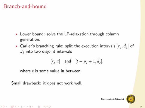
Branch-and-bound

I Lower bound: solve the LP-relaxation through columngeneration.

I Carlier’s branching rule: split the execution intervals [rj , d̄j ] ofJj into two disjoint intervals

[rj , t] and [t− pj + 1, d̄j ],

where t is some value in between.

Small drawback: it does not work well.

25

Successful: Time indexed ILP with lower bound

Use binary variables xjt to indicate whether job J = j starts attime t. Then solve the ILP

min Lmax

subject to

‘Do not use more than m machines’‘Start each job exactly once’

‘Obey release dates, deadlines, and precedence constraints’‘Lateness job Jj ≤ Lmax’

‘All xjt are binary’

Crucial additional inequality: Lmax ≥ L + 1.

26

Great combination

I The column generation algorithm can easily prove infeasibility,but has problems finding m feasible single-machine schedulesthat cover all jobs exactly once.

I CPLEX can find the required m feasible single-machineschedules, but it has difficulty proving the lower bound.

I Hence, the combination of the two has it all.

27

Computational results

Up to 180 jobs with 9 machines. Processing times from U [1, 20].Precedence constraints of the ≥ type only.

I The lower bound is always tight (in our experiments).

I Problems with more than 20 jobs per machine get hard (areat the limit of 30 minutes).

I Using local search for the pricing problem speeds up thealgorithm a lot.

I Doubling the processing times does not increase the runningtimes too much on average, but some instances take a lotmore time.

28

Enhancements (1)

The time indexed formulation is quite big. Cut down the executioninterval for each job heuristically:

Use the knowledge obtained from the lower bound procedure: lookat the solution that solves the LP-relaxation for the problem withLmax ≤ L + 1 using no more than m machines.

Increase the release date of job Jj to the smallest start timeoccurring in that solution. Similarly, reduce the deadline of job Jj

to the largest completion time in that solution.

Optimality is only guaranteed if a solution with value L + 1 isdetermined. For ≥ precedence constraints this is always the case.It reduces the running times by a factor 8 (on average).

29

Enhancements (2)

Equality (no-wait) precedence constraints make the problem hardto solve (but they are needed in for the RCPS problem).

Compute the difference in starting time between jobs Ji and Jj

required to satisfy the no-wait constraint. For each pair t and t′

satisfying this difference add the valid inequality

xi,t = xj,t′ .

Now several instances can be solved that could not be solved withinthe 30 minute time limit before; it reduces the running times by alarge factor. Specifying the lower bound on Lmax is still crucial.

30

Resource constrained project scheduling (RCPS)

Strongly related to the parallel machine scheduling problem.Equal in RCPS and parallel machine scheduling:

There are n jobs J1, . . . , Jn with

I processing time pj (≥ 0);

I due date dj (can be negative);

I release date rj (≥ 0);

I deadline d̄j .

There can be precedence constraints of the form:

I Jj must start at least X time units after Ji;

I Jj must start exactly X time units after Ji;

I Jj must start at most X time units after Ji.

31

RCPS (2)

Differences between RCPS and parallel machine scheduling:

Instead of machines there are resources.

I To execute a job, you need a given amount of each one of theresources during each time unit (resource consumptionpattern).

I The availability of resources can vary over time.

In fact: parallel machine scheduling is a special case of RCPS

I only one kind of resource needed for processing a job.

I the available amount of resource amounts to m at all times.

I each job constantly needs 1 unit of resource during itsexecution.

The standard objective function in RCPS is Cmax.

32

Varying resource availability

The problem setting is the same as the parallel machine schedulingproblem, but the number of available resources (machines) variesover time.

m

r1 d̄1r2 d̄2 r3 d̄3 Time

Dummy jobs: completion times get fixed such that they block themachine for the ordinary jobs.

33

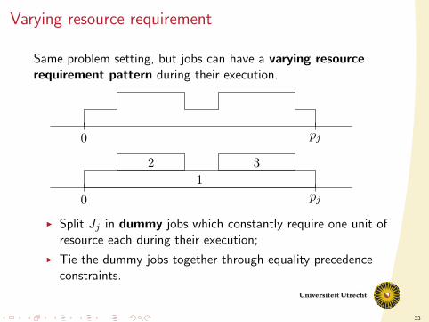
Varying resource requirement

Same problem setting, but jobs can have a varying resourcerequirement pattern during their execution.

0 pj

12 3

0 pj

I Split Jj in dummy jobs which constantly require one unit ofresource each during their execution;

I Tie the dummy jobs together through equality precedenceconstraints.

34

Multiple resource types

Assumptions (for simplicity of presentation)

I 2 types of resources: available quantities m1 and m2;I each job constantly requires either

� 1 unit of resource type 1 (set R1)� 1 unit of resource type 2 (set R2)� 1 unit of both resource types (set R1,2)

I There are no precedence constraints.

Jobs in R1,2 are split into two single-resource jobs, which areconnected by an equality precedence constraint.

The resulting single-resource jobs are independent, except for theequality precedence constraints. We must find ≤ m1 and ≤ m2

feasible machine schedules for the jobs requiring resources 1 and 2,such that the precedence constraints are met.

35

ILP-model

Use S and V to denote the feasible machine schedules forresources types 1 and 2. Use ajs and bjv tot indicate whether Jj isincluded in s and v.

min∑s∈S

xs +∑v∈V

yv subject to

∑s∈S

ajsxs = 1, for each j ∈ R1 ∪R1,2∑v∈V

bjvyv = 1, for each j ∈ R2 ∪R1,2∑s∈S

Sjsxs −∑v∈V

Sjvyv = 0, for each j ∈ R1,2∑s∈S

xs ≥ m1

∑v∈V

yv ≥ m2

xs, yv ∈ {0, 1} ∀s ∈ S, v ∈ V.

36

Necessary adjustments

Solve the LP-relaxation using column generation: is there asolution with value m1 + m2?

I we must solve two separate pricing problems (but they are justlike before)

I we can still use the time-indexed ILP

I the intermediate lower bound becomes a bit more complicated

Intermediate lower bound:

((c∗2 − c∗1 + µ0 − λ0)m2 +∑

j∈R1∪R1,2λj +

∑j∈R2∪R1,2

µj

(1− c∗1 − λ0)

if c∗1 + λ0 < c∗2 + µ0 (similar expression otherwise).

37

Other extensions

Operator scheduling:A job needs an operator to start it up, which takes 1 time unit.The same analysis can be used.

Set-up times and change-over times.The same analysis applies, but in case of sequence-dependentchange-over times, the time-indexed formulations cannot be usedanymore.

Unavailability and planned maintenance on specific machines.Use set Di of dummy jobs to mimic the unavailability of a machineMi. The problem is to get Di on one machine completely. Pricingproblem etc. goes unchanged, but the time-indexed formulationcannot be applied anymore.

38

Conclusions and future research

I Column generation gives strong bound.

I The strenght of CPLEX, when knowing the ‘optimum’, isprobably due to its preprocessing engine, which usesConstraint Satisfaction techniques.

Explore the combination of ILP-techniques and ConstraintSatisfaction.