using an activity-based model to explore possible impacts...

USING AN ACTIVITY-BASED MODEL TO EXPLORE

POSSIBLE IMPACTS OF AUTOMATED VEHICLES

Suzanne Childress

(Corresponding Author)

Senior Modeler

Puget Sound Regional Council

1011 Western Ave., Suite #500

206-464-7090

[email protected]

Brice Nichols

Associate Modeler



206-464-7090

[email protected]

Billy Charlton

Program Manager



206-464-7090

[email protected]

Stefan Coe

Senior GIS Analyst



206-464-7090

[email protected]

August 1, 2014

Submitted for presentation at the Transportation Research Board 2015

Annual Meeting, Washington, D.C.

mailto:[email protected]




Childress, Nichols, Charlton, Coe 1

ABSTRACT 1

Automated vehicles (AV) may enter the consumer market with various stages of automation in 2 ten years or even sooner. Meanwhile, regional planning agencies are envisioning plans for time 3

horizons out to 2040 and beyond. To help decision-makers understand the impact of this 4 technology on regional plans, modeling tools should anticipate automated vehicles’ effect on 5 transportation networks and traveler choices. This research uses the Seattle region’s activity-6 based travel model to test a range of travel behavior impacts from AV technology development. 7 The existing model was not originally designed with automated vehicles in mind, so some 8

modifications to the model assumptions are described in areas of roadway capacity, user values 9 of time, and parking costs. Larger structural model changes are not yet considered. Results of 10 four scenario tests show that improvements in roadway capacity and in the quality of the driving 11 trip may lead to large increases in vehicle-miles traveled, while a shift to per-mile usage charges 12

may counteract that trend. Travel models will need to have major improvements in the coming 13 years, especially with regard to shared-ride, taxi modes, and the effect of multitasking 14

opportunities, to better anticipate the arrival of this technology. 15


INTRODUCTION 16

Automated vehicles (AVs) are under development by major car manufacturers and technology 17 firms, and may enter the consumer market with various stages of automation in ten years or even 18

sooner (KPMG and CAR 2014). Meanwhile, regional planning agencies are envisioning plans 19 for time horizons out to 2040 and beyond. Within the time horizon of the plans, AVs may 20 significantly alter transportation choices, impacting regions’ planning goals. To understand 21 future travel patterns, modeling tools should anticipate automated vehicles’ impact on 22 transportation networks and traveler choices. 23

24 In the latest long-range regional plan, the Puget Sound Regional Council (PSRC) (2010) 25 established goals to guide the region toward healthy growth, including: 26 27

improving safety and mobility, 28 reducing greenhouse gas emissions and congestion, 29

focusing growth in already urbanized areas to create walkable, transit oriented 30 communities, 31

preventing urbanization of rural and resource lands, and 32

helping people live happier and more active lives. 33 34

These goals reflect statewide legislation from Washington State’s Growth Management Act as 35 well as federal aims outlined in Moving Ahead for Progress in the 21st Century Act (MAP-21). 36 Self-driving cars could impact all these focus areas, so anticipating their adoption is imperative 37

to maintaining timely and informed regional plans. 38 39

This paper considers modeling techniques to measure the impacts of self-driving cars using an 40

activity-based model, and explores how modeling capabilities must be improved to better answer 41

questions related to this new technology. Since there is so much uncertainty around the future of 42 AVs, several model scenarios are created to consider broad impacts of self-driving vehicle 43

adoption in the Puget Sound region of Washington State. These scenarios clearly stretch current 44 model capabilities, and depend on highly uncertain inputs. However, it is still useful to test the 45 existing models in order to start a conversation with planners and decision-makers, as well as to 46 highlight shortcomings in our existing methods to modelers. The aim of this paper is not to 47

accurately predict the future impacts of automated vehicles, but rather to develop appropriate 48 ways of evaluating a range of potential impacts on regional transportation. 49 50

BACKGROUND 51

Automated vehicles could drastically change traffic flow, up-ending long-held assumptions 52 about maximum roadway capacity and volume-delay functions. Vehicle-to-vehicle coordination 53

systems allow cars to travel with much shorter headways, enabling higher volumes at high 54 speeds. If AVs also reduce collision rates, non-recurrent congestion would decrease as well. 55 FHWA (2013) estimates that 60% of all congestion is attributed to non-recurring sources such as 56 crashes and other vehicle-roadway mishaps, suggesting that a safer, more coordinated fleet could 57 reduce delay and support more consistent travel times. Even partially-autonomous vehicle 58 capabilities may increase roadway capacity. Tientrakool et al.(2011) estimate that highway 59


capacity could be increased by 43% using vehicle sensors and up to 273% with vehicle-to-60

vehicle communications. Shladover et al. (2013) estimate that vehicle-to-vehicle coordination of 61 adaptive cruise control could increase capacity by 21% with 50% of all vehicles using the 62 technology, or up to 80% capacity increase with a 100% coordinated vehicle fleet, based on 63

empirical testing. Fernandes and Nunes (2012) estimate that capacity could increase as much as 64 five-fold for platoons traveling around 45 miles per hour. More efficient fleets could be 65 represented as additional roadway capacity, which can be represented very easily in existing 66 travel models. 67 68

To date, few regional-scale modeling efforts have addressed potential impacts of AVs. Gucwa 69 (2014) tested some capacity-altering assumptions on regional VMT in the San Francisco Bay 70 Area using the Metropolitan Transportation Commission’s activity-based travel model. Gucwa’s 71 results suggest that doubling capacity only increases region-wide VMT by around 1%, but does 72

significantly reduce peak congestion. Gucwa found that changing users’ values of time had much 73 more impact on VMT than capacity changes, and estimated the Bay Area’s VMT would increase 74

between 8% and 24%, depending on how automated vehicles users’ time values changed. 75 76

Gucwa’s findings suggest that changes in user behavior may have large effects on regional travel 77 as vehicle fleets become more automated. Gucwa, and many others, assume that being driven by 78 a robotic vehicle will eventually be less stressful than piloting one’s self through concentration-79

demanding and chaotic congestion, thus making travelers less averse to in-vehicle time. Rather 80 than focusing on complicated navigation skills, travelers could spend time relaxing or working, 81

perhaps reducing the disutility placed on travel time. Since AVs are a new technology, the exact 82 influence of such attributes relative to travel time in these vehicles is unknown. However, these 83 factors are similar in nature to non-traditional transit attributes that often contribute to both mode 84

choice and route choice (Outwater et al. 2013). These attributes, such as comfort, reliability and 85

amenities like Wi-Fi, have proven difficult to explicitly represent in travel models. Instead, 86 through empirical methods, travel models can represent the utility associated with these 87 attributes through adjustments in travel time. Similarly, we can attempt to model the behavioral 88

changes that may arise from AVs by making assumptions about the equivalent perceived travel 89 time reductions that may result from ancillary factors. 90

91 Many other aspects of AV technology may affect traveler behavior as well, including costs, 92

vehicle availability and ownership, and parking price and location. Since more technical 93 infrastructure will be required to operate and manage self-driving cars, usage could more easily 94 be tracked per mile, making VMT-based taxes and pay-as-you-drive insurance policies more 95 realistic policy tools for personal vehicles. This pricing strategy could reduce overall VMT, as 96 frequently-forgotten fixed costs such as insurance, licensing, and registration fees are replaced 97

with more transparent marginal costs for every trip (Parry and Small 2005, Nichols and 98 Kockelman 2014). Shared autonomous vehicles would likely offer per-mile rates as well, 99

echoing existing business models from hired rideshare services like Uber and Lyft. Shared AVs 100 may become a popular service, since on-demand automated pickups would reduce the need to 101 own and thus store a personal vehicle. Depending on the technology’s development, many could 102 find owning a personal driverless vehicle too costly, relying on occasional pickups by shared 103 automated vehicles. 104 105


AVs may reduce the need for close-by parking as vehicles could conceivably self-park in 106

cheaper, more distance parking locations (Fagnant and Kockelman 2013). This behavior could 107 alter fixed costs at trip ends, reducing driving costs that lead to mode shifts or more automobile 108 travel to areas with high parking cost. Aside from altering destination choices and mode choice, 109

this behavior may also increase VMT as empty vehicles are sent for pickup and parking by 110 owners or users in a shared system. Some of these impacts can be easily modeled by simply 111 reducing parking costs in all zones, but accounting for increased VMT requires more knowledge 112 on parking cost, location, and trip tour timing. 113 114

VMT will likely increase as new users and more (perhaps longer) trips are induced from more 115 efficiently-operated roadways. Baseline demand consistently increases after congestion is 116 reduced with capacity expansion or operational improvements (see Cervero 2001 and Litman 117 2014b for meta-analyses of induced travel studies). Additionally, as in-vehicle time is less 118

stressful, travelers may be willing to tolerate slower travel times and longer travel distances, 119 adding more congestion still. 120

121 Fully autonomous vehicles may provide new mobility opportunities to those unable or unwilling 122

to drive a vehicle themselves, especially unlicensed young people, the physically impaired, and 123 some senior citizens. These user groups may be able to make more trips, access more 124 destinations, and rely on modes other than shared rides, public transit, and taxi. The amount of 125

additional mobility provided by AVs depends on mode shifts for non-drivers. Affordable, 126 competitive trips provided by a personal or shared AV would likely improve the opportunities a 127

non-driver could access, especially in more suburban, automobile-oriented contexts. Recognizing 128 how different groups are affected by AV developments is important to understanding regional 129 mobility and accessibility to jobs and resources. 130

131

Altogether, impacts of autonomous vehicles are highly speculative. Future impacts depend on 132 technological development, market reactions, and regulatory actions, making it challenging to 133 confidently predict impacts to regional transportation systems. With so many unknown and 134

potential effects of AVs, it is challenging to anticipate long-term effects with certainty. However, 135 some of these impacts should be considered early on, to understand model sensitivity and 136

develop feasible analysis boundaries. With these analyses, agencies can prepare more dynamic 137 long-range plans, by defining and evaluating some rational futures and exploring most likely 138

scenarios as technologies appear and mature. 139 140

MODEL SCENARIOS 141

To model potential impacts from automated vehicles in the Puget Sound region, four scenarios 142

are considered. The following sections explore ways to model some of the impacts mentioned 143

above and to provide guidance for other regions interested in planning for automated vehicle 144 futures. 145 146 PSRC’s activity-based travel model, called SoundCast, was applied to test the possible impacts 147 of automated vehicles. SoundCast includes a travel demand component written in the Daysim 148 software. SoundCast simulates individual travel choices across a typical day (PSRC 2014). These 149


choices include long-term choices like work location and auto-ownership, as well as shorter-term 150

choices like mode choice and route choice. Inputs to the model include parcel-based locations of 151 households and jobs, and highway and transit networks. 152 153

The scenarios have all been modeled using the base year of 2010, to avoid forecasting market 154 penetration scenarios or speculation on business models or technology development over time. 155 Using the most recent base year also helps focus the analysis directly on AVs, and avoids 156 uncertainties in future growth and changes to the transportation system. This isolation is useful to 157 understand some model behaviors and helps develop basic guidelines for evaluating automated 158

vehicles. As these analyses mature, future years should be evaluated for more comprehensive 159 case studies. 160 161 These scenarios explore how driverless cars can influence demand through changes in capacity, 162

perceived travel time, parking cost, and operating cost. They are described separately below. 163 164

Scenario 1: Increased Capacity 165

166 “AVs use existing facilities more efficiently.” 167

168 The first scenario reflects operational improvements from full or partial vehicle automation. This 169

scenario is modeled by increasing the hourly capacity coded on roadway network links and 170 captures one major impact of AVs on a roadway network. While it’s currently unclear what 171 magnitude of capacity increase is likely, based on cited research a 30% increase represents a 172

modest result from AV adoption. All freeway and major arterial capacities are increased by 30%. 173

174

Scenario 2: Increased Capacity and Value of Time Changes 175

176 “Important trips are in AVs.” 177

178 Scenario 2 builds upon the first scenario by assuming that, along with capacity improvements 179 from AV use, individuals using the AVs will perceive the time in them less negatively than time 180 spent driving in regular vehicles. The scenario envisions the point in time that AVs have only 181 been partially adopted, and only by higher income households. As with many new technologies, 182

the initial price will most likely only be attractive to higher income households. Considering that 183 the current cost of self-driving GPS technology alone is around $70,000, (KPMG and CAR 184 2012) adoption may be among high-income households for some time to come. This assumption 185

follows existing adoption patterns of more expensive cutting-edge vehicles such as hybrid and 186 electric vehicles. For example, Hjorthal, (2013) showed that early adopters of electric vehicles 187 were households with high income, owning more than one car, and used mainly to complement a 188 conventional car for commutes. Petersen and Vovsha (2005) found that higher income house-189

holds tend to utilize newer vehicles, and among household members, the new vehicles are 190 allocated to workers at a higher rate than retirees and school children of driving age. A similar 191 trend might initially occur with AVs adoption. High income households might purchase one of 192


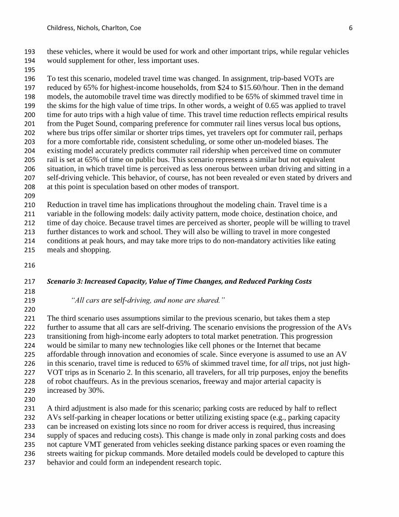
these vehicles, where it would be used for work and other important trips, while regular vehicles 193

would supplement for other, less important uses. 194 195 To test this scenario, modeled travel time was changed. In assignment, trip-based VOTs are 196

reduced by 65% for highest-income households, from $24 to $15.60/hour. Then in the demand 197 models, the automobile travel time was directly modified to be 65% of skimmed travel time in 198 the skims for the high value of time trips. In other words, a weight of 0.65 was applied to travel 199 time for auto trips with a high value of time. This travel time reduction reflects empirical results 200 from the Puget Sound, comparing preference for commuter rail lines versus local bus options, 201

where bus trips offer similar or shorter trips times, yet travelers opt for commuter rail, perhaps 202 for a more comfortable ride, consistent scheduling, or some other un-modeled biases. The 203 existing model accurately predicts commuter rail ridership when perceived time on commuter 204 rail is set at 65% of time on public bus. This scenario represents a similar but not equivalent 205

situation, in which travel time is perceived as less onerous between urban driving and sitting in a 206 self-driving vehicle. This behavior, of course, has not been revealed or even stated by drivers and 207

at this point is speculation based on other modes of transport. 208 209

Reduction in travel time has implications throughout the modeling chain. Travel time is a 210 variable in the following models: daily activity pattern, mode choice, destination choice, and 211 time of day choice. Because travel times are perceived as shorter, people will be willing to travel 212

further distances to work and school. They will also be willing to travel in more congested 213 conditions at peak hours, and may take more trips to do non-mandatory activities like eating 214

meals and shopping. 215

216

Scenario 3: Increased Capacity, Value of Time Changes, and Reduced Parking Costs 217

218 “All cars are self-driving, and none are shared.” 219

220

The third scenario uses assumptions similar to the previous scenario, but takes them a step 221 further to assume that all cars are self-driving. The scenario envisions the progression of the AVs 222

transitioning from high-income early adopters to total market penetration. This progression 223 would be similar to many new technologies like cell phones or the Internet that became 224 affordable through innovation and economies of scale. Since everyone is assumed to use an AV 225 in this scenario, travel time is reduced to 65% of skimmed travel time, for all trips, not just high-226

VOT trips as in Scenario 2. In this scenario, all travelers, for all trip purposes, enjoy the benefits 227 of robot chauffeurs. As in the previous scenarios, freeway and major arterial capacity is 228 increased by 30%. 229 230 A third adjustment is also made for this scenario; parking costs are reduced by half to reflect 231 AVs self-parking in cheaper locations or better utilizing existing space (e.g., parking capacity 232 can be increased on existing lots since no room for driver access is required, thus increasing 233

supply of spaces and reducing costs). This change is made only in zonal parking costs and does 234 not capture VMT generated from vehicles seeking distance parking spaces or even roaming the 235 streets waiting for pickup commands. More detailed models could be developed to capture this 236

behavior and could form an independent research topic. 237


Scenario 4: Per-mile Auto Costs Increased 238

239 “"All autos are automated, with all costs of auto use passed onto the user.” 240 241 The final scenario considers a counterpoint situation in which AVs have become so common, 242

and shared AVs systems so effective, that personal AV ownership is no longer necessary. 243 Mobility is perhaps treated as a public utility, where all trips are provided by a taxi-like system at 244 a set rate. In this scenario, vehicles and road use are priced by a combination of industry and 245 government to cover infrastructure operation and maintenance costs. The scenario assumes that 246 all costs of driving are passed on to the user. The cost components that would be included under 247 such a scenario are: vehicle parking, vehicle and infrastructure maintenance, accidents, road 248 construction, vehicle cost, and negative externalities like congestion, air pollution, and global 249 warming. It is assumed that the system provides the same service as a personal automobile, but 250

comes at a higher per-mile rate. A rate of $1.65/mile was chosen to reflect total user and system 251 auto per mile costs and current ride-sharing taxi services. Litman (2007) estimated that the cost 252 per auto mile in urban area during the peak period was about $1.51 per mi. Furthermore 2014 253 per-mile price from Uber (2014) in Seattle was $1.65. The per-mile costs are a large increase 254

from current total costs of around 60 cents/mile (AAA 2013) and much larger than marginal 255 driving costs of 15 cents in PSRC’s model. 256

257 No capacity increase is assumed in this scenario, to reflect a worst-case scenario in which the 258 AVs provide no additional capacity (perhaps due to regulations preventing close car following, 259

for example). Table 1 summarizes these four scenarios for quick reference. 260 261

Table 1. Scenario Definitions. 262 263

264

265 266

Scenario 1 Scenario 2 Scenario 3 Scenario 4

"AVs increase network

capacity."

"Important trips are in

AVs"

"Everyone who owns a car

owns an AV."

“"All autos are automated,

with all costs of auto use

passed onto the user.”

30% capacity increase on

freeways, major arterials





Travel time is perceived at

65% of actual travel time

for high value of time

household trips (>$24/hr.)

Travel time is perceived at

65% of actual travel time

for all trips

50% parking cost reduction

Cost per mile is $1.65


RESULTS 267

The model outputs from Scenarios 1-4 are compared to the 2010 baseline to investigate the 268

potential impacts of the new technology. Table 2 shows the scenario results for typical measures 269

output by travel models. All the scenarios with a capacity increase indicate increased vehicle 270

miles travelled (VMT), ranging from around 4 % to 20%. However, only one of the three 271

capacity-increase scenarios showed an increase in vehicle hours traveled (VHT). In the first two 272

scenarios, the additional network capacity offsets the additional vehicle miles by allowing 273

vehicles to travel at a faster speed. In the third scenario, however, the reduction in perceived 274

travel time on all trips to 65% of the actual time, along with reduced parking costs induced so 275

much additional demand that the benefits from increase in capacity was offset. 276

Table 2. Scenario Results, Base Year 2010, Summaries by Average Travel Day. 277

278 279 280 Note that in all three of the capacity-increase scenarios the average network speed is higher than 281 the base scenario by about one or two miles per hour. The vehicle-hours of delay are reduced by 282

Measure Value Base 1 2 3 4

VMT Total Daily 78.7 M 81.5 M 82.6 M 94.1 M 50.8 M

% Change --- 3.6% 5.0% 19.6% -35.4%

(Versus Base)

VHT Total Daily 2.82 M 2.72 M 2.76 M 3.31 M 1.67 M

% Change --- -3.9% -2.1% 17.3% -40.9%

Trips Trips/Person 4.1 4.2 4.2 4.3 4.1

Distance Average Trip Length 6.9 7 7.2 7.9 5.8

(miles) Work Trips 12.4 12.9 12.9 20 11.5

School Trips 5.8 5.8 5.8 6.7 4.7

Delay Daily Average 846.0 700.0 727.2 996.1 350.2

(1000 hours) Freeways 288.1 201.2 218.3 338.7 56.4

Arterials 557.9 498.8 508.9 657.5 293.8

Speed Daily Average 27.9 30 29.9 28.4 30.4

(mph) Freeways 40 44.7 44.2 40.8 49.2

Arterials 22.5 23.2 23.1 22.3 24.3

Mode SOV Share 43.7 43.7 42.7 44.8 28.7

(%) Transit Share 2.6 2.7 2.7 2.4 6.2

Walk Share 8.6 8.6 8.4 6.8 13.1


about 150,000 vehicle hours in the first scenario and 100,000 vehicle hours in the second 283

scenario, but VHT and delay are both increased in Scenario 3 as VMT increases nearly 20%. 284 This surge in VMT corresponds to about 150,000 hours extra delay and about 17% more vehicle 285 hours. The increase in delay reflects the system-wide assumption of reduced perceived travel 286

time, where people are less averse to delay and thus more willing to tolerate congestion. 287 288 The additional vehicle miles result mostly from an increase in the number of trips and an 289 increase in the length of the trips. SoundCast includes sensitivity to travel time in the daily 290 activity pattern, exact number of tours, and intermediate stop models that predict the number of 291

trips people take. As perceived and actual travel time is reduced, the number of trips people will 292 take will increase because of a negative coefficient on travel time. For trip lengths, the 293 destination choice models have a negative coefficient on travel time, so users will travel farther if 294 the perceived travel time is reduced. In Scenario 3, average distance to work increases 295

dramatically to 20.0 miles, from a base of 12.4 miles. Much of this increase may be due to some 296 curious geographical quirks of our region: with less onerous drive time, some drivers may be 297

choosing to follow a circuitous path around Puget Sound instead of utilizing the shorter car-ferry 298 option across the Sound into downtown Seattle. In this scenario, total vehicle miles also increase 299

as travelers switch modes from transit and walking to single occupancy vehicles; transit shares 300 decrease around 9% and walk shares decline 21%. 301 302

Scenario 4 serves as counterpoint to Scenarios 1-3, to explore other ways in which AV could 303 affect regional transportation. This scenario is optimistic towards AV adoption and use; shared 304

AVs make owning a vehicle unnecessary, but travel is priced rather high (up to $1.65 per mile 305 versus 15 cents in the base), such that many trips are suppressed or trip lengths shortened. 306 Pessimism is assumed for operational benefits; AVs are thought to be used so widely in this 307

scenario that operational benefits are saturated, and no capacity increases are realized. If 308

increased per-mile costs were applied to all trips, model results suggest VMT may be reduced as 309 much as 35% versus the base. Vehicle-hours are similarly reduced by over 40%. Though 310 numbers of trips per person are very similar across all scenarios, Scenario 4 indicates travelers 311

will generally opt for shorter trips – average trip lengths are down 15% versus the base and over 312 25% less than Scenario 3, where average trip lengths are the longest of all scenarios. Scenario 4 313

results also suggest taxi-like pricing would cut drive-alone mode shares by a third, while transit 314 and walk modes might increase by 140% and 50%, respectively. Though some travel could be 315

suppressed in this scenario, the overall network performs better than the base or any other 316 scenario. Delay is less than half that in the baseline, and freeway speeds are nearly 10 mph faster 317 than the base. 318 319 Further analysis of tour lengths was performed. Table 3 shows the percent difference in tour 320

lengths by purpose when comparing Scenario 1 to Scenarios 3 and 4. Escort tours had the 321 greatest sensitivity to the modeled time and cost changes among the scenarios. When comparing 322

average escort tour lengths from the base scenario, Scenario 3 showed a 24% increase and 323 Scenario 4 had a 51% decrease. Because escort tours involve more travelers in the same vehicle, 324 they have a higher value of time than other tours. This higher value of time translates to a 325 greater sensitivity to travel time changes, and thus shorter tour lengths in Scenario 3. Scenario 326 4’s decrease comes from sensitivity to cost per mile of these tours. 327 328


Figure 1. Percent Difference in Tour Lengths: Scenario 1 Compared to Scenarios 3 and 4 329

330

331 332

Geographic Distribution of Results 333

Aside from aggregate system performance, model results were used to provide insight into the 334 spatial distribution of possible effects from AV. Figure 2 visualizes geographic distribution 335

results of the most “aggressive” automated car future, Scenario 3. In this analysis, an 336 accessibility metric called “aggregate tour mode-destination logsums,” or simply “aggregate 337 logsums,” is used. Aggregate logsums are household-based measures of accessibility, calculated 338

as the sum of the expectation across all possible locations, across all modes (Bowman and 339

Bradley, 2006). The aggregate logsums are calculated separately for households grouped by 340 income, vehicle availability, and transit accessibility, and separately by purpose. A fairly typical 341 household type was selected for analyses in Figures 2: a medium-income household located 342

within ¼ - ½ mile of transit, owning some vehicles, but fewer vehicles than adults. Aggregate 343 logsums are an index measure, and do not have much meaning by themselves, but can be used to 344

compare the differences between two scenarios. 345 346

Figure 2 shows that with capacity increases and a reduction in the perception of travel time as in 347 Scenario 3, perceived accessibility would be higher for most households, but especially higher 348 for more remote, rural households. Note that perceived accessibility increases for all households, 349 but especially for households in less urban areas. Two groups were selected to analyze how 350 different income groups would be impacted: one low income group and one high income group. 351

For the low income group, the percent change in aggregate logsums was 8.5% between the base 352 scenario and Scenario 3. For the high income group, the percent change in aggregate logsums 353

was about the same at 8.9% between the base scenario and scenario 3. The modest difference 354 between the low and high income groups difference in logsums indicates that with the scenario 355 as designed, low income populations experience nearly the same increase in accessibility as 356 higher income groups. 357

358


Figure 2. Accessibility Increase: Scenario 3 minus Base. 359

360

361

This result suggests that AVs, as modeled with assumptions in Scenario 3, would not reduce 362 access for any specific group and would actively increase accessibility in regions away from the 363 typically highly-accessible urban core. Scenario 3 assumes that driving is easier (increased 364 capacity), cheaper (lower parking costs), and more enjoyable (perceived travel time decreases) 365

for all users, leading to a jump in accessibility benefits directly through personal vehicle trips. 366 Though many Puget Sound residents would enjoy higher accessibility in this scenario, total VMT 367

climbs nearly 20%, possibly compromising the region’s goals of reducing greenhouse gas 368 emissions and containing growth into existing urban areas. Figure 3 shows how these VMT 369

increases are dispersed across the region. 370

371


372

Figure 3. Scenario 3, Estimated Changes in Average Daily VMT per Person over base 373

374

375

This result indicates that average VMT per person in nearly all zones would increase, with the 376

most extreme increases occurring in outlying areas, and even in some core zones of central 377 Seattle and Bellevue. Zones decreasing in VMT are generally sparsely-populated with few 378 samples to properly estimate. Improving regional mobility is one of PSRC’s goals, but such 379 improvements made through increased personal vehicle trips may be conflicting with 380

environmental and land-use targets. 381

DISCUSSION and RECOMMENDATIONS 382

Planning Implications 383

These results imply that AVs could both help and hinder PSRC’s policy goals. Speed and 384 capacity increases may improve regional mobility, but they also could induce additional demand, 385 leading to more VMT, and hence greater greenhouse gas emissions. If, on the other hand, a 386

greater share of AVs are electric than would have been otherwise, greenhouse gas emissions 387 could possibly fall. Reducing perceived travel time may provide a more enjoyable traveling 388 experience, but could facilitate longer trips and more VMT. The model runs show that 389


improvements in vehicle hours of delay from capacity expansion can easily be offset by the 390

reduction in perceived time. The amount of additional network capacity this technology can 391 provide is unknown, as are behavioral reactions of travelers. These analyses simply show that a 392 range of reasonable assumptions about AV adoption could have quite different impacts on 393

regional transportation. For example, if self-driving cars are priced per mile, both vehicle miles 394 travelled and vehicle hours travelled could be greatly reduced, by as much as 20 and 30%, 395 respectively, with SOV shares declining 40% and transit shares almost doubling. Conversely, 396 model assumptions in the first three scenarios indicate potential for much more VMT and delay, 397 with more people carried in SOVs, generally worse or equivalent network performance, but 398

higher mobility overall. 399 400 Self-driving vehicle adoption impacts are addressed in this paper from the perspective of PSRC’s 401 long-range plan goals of mobility, accessibility, and congestion impacts, but future research 402

should explore potential safety, emissions, and land use changes. Many simplifying assumptions 403 were used to isolate and test network and behavioral changes potentially associated with 404

automated technology development. However, if AV use does dramatically change regional 405 VMT, trip lengths, and mode shifts, it follows that land uses may shift dramatically as well. 406

Understanding these built environment changes will be very important in planning for future 407 impacts of AV technology. 408 409

Modeling Implications 410

Some improvements to this study’s methodology are achievable now, such as testing future-year 411

settings and linking the travel and land use models. These are perhaps the next logical next steps 412 in more detailed AV analyses, since changes in accessibility may be quite large and those 413 accessibility changes would impact land use development patterns. 414

415

More importantly, existing tools are demonstrably not sufficient for expressing the full range of 416 possibilities that automated vehicles may present. This study makes oversimplifications, such as 417 using a present-year land use assumptions and assuming broad AV costs and user values of time. 418

The model was estimated and calibrated against data that represents today’s network reality, 419 which is far outside of the reality that may exist with wide AV adoption. The challenges faced in 420

modeling AV scenarios highlight limitations of today’s tools in addressing this technology. 421 Many modeling improvements are considered below. 422

423 424 The future business model for shared AVs is entirely opaque. At a minimum, this could be 425 represented more directly with a top-tier taxi mode, which SoundCast currently lacks. Most 426 recent travel surveys indicate growing shares for taxi and taxi-like trips from ridesharing 427

services. Including a taxi mode would allow modelers to tweak performance and prices specific 428 to shared AVs. This would go a long way toward preparing our model for outcomes where many 429

of us may have robotic chauffeurs. 430 431 In activity-based models, household-owned AVs could be represented as a separate mode from 432 non-automated vehicles with their own modal constants and variables. Representing AVs as a 433 separate mode may be necessary if policy makers would like to consider separated lanes for 434


AVs. As with high-occupancy vehicles and toll links, AVs may need to be modeled using a 435

separate set of user classes with unique values of time and network link attributes. 436 437 The reduction in perceived travel time in AVs would be better modeled by attributing the 438

improvement in experience of travel time to actual measurable variables, as has been researched 439 with transit (Outwater, 2013). In mode and destination choice models, the stages of automation 440 could be a set of zero-one variables for the AV mode; assuming that the AV mode would 441 become more attractive with more automation and that with more automation, travel impedance 442 variables would have lower coefficients. 443

444 Currently, modelers lack the evidence to add AV-related alternatives and variables into travel 445 demand models. Because these vehicles do not yet exist but modelers need to incorporate their 446 possible impacts on travel demand, the most straightforward way to understand behavior would 447

be to conduct a stated preference survey. 448 449

A stated preference survey about travel behavior using AVs should try to answer some of the 450 following questions: 451

452

How much would different types of people be willing to purchase different levels of 453 automation and for what price? 454

Who would prefer to use the AVs as a shared service, and forgo car ownership? 455

How will people perceive and value their time differently in AVs? 456

Would people anticipate moving farther away from work? 457

Would businesses choose to locate farther from the city center? 458

What aspects of the AVs would cause people change their behavior most such as ability 459 to work, avoiding congestion, or safety? 460

461

Stepping further back and thinking about more than just variables and their coefficients, there are 462 some real shifts in how people perceive travel even today that our models simply don’t capture. 463

Multitasking (e.g. reading/emailing on a smartphone while on the bus), the effect of ingrained 464 habits and “lifestyle choices” (e.g., a person who really loves driving their luxury car, or another 465 person who would never consider driving to work even if it had free parking) need to be 466

incorporated in the next generation of models. Those types of high-level differences will be 467 amplified when a disruptive technology like AVs are introduced. 468 469

Closing Remarks 470

For modelers and policymakers alike it’s important to remember that, when presented with 471 automated vehicle technology, people are still going to behave based on the options available to 472

them and on the constraints they face in their daily lives. We have tried to lay out reasonable (or 473 at least conceivable) scenarios in this study, but the future may be more different than we’ve 474 envisioned. That possibility makes it even more critical that we improve our tools now to support 475 the policymakers and planners who will have to grapple with this new technology. 476

477 This research is just a starting point. We hope to continue the discussion as we sharpen our 478 predictive tools in the coming years. 479


REFERENCES 480

AAA (2013) Your Driving Costs. https://exchange.aaa.com/wp-content/uploads/2013/04/Your-481 Driving-Costs-2013.pdf 482 483 Anderson, J., N. Kalra, K. Stanley, P. Sorensen, C. Samaras, O. Oluwatola (2014) Autonomous 484 Vehicle Technology: A Guide for Policymakers. RAND Institute. 485

http://www.rand.org/content/dam/rand/pubs/research_reports/RR400/RR443-1/RAND_RR443-486 1.pdf. 487 488 Bowman, John L. and Mark Bradley (2008), Activity-based models: approaches used to acheive 489 integration among trips and tours throughout the day. European Transport Conference, 490

Leeuwenhorst, The Netherlands, October, 2008. 491 http://www.jbowman.net/papers/2008.Bowman_Bradley.Approaches_to_integration_ETC.pdf 492

493

Burns, L., W. Jordan, B. Scarborough (2013) Transforming Personal Mobility. The Earth 494

Institute, Columbia University. 495 http://sustainablemobility.ei.columbia.edu/files/2012/12/Transforming-Personal-Mobility-Jan-496

27-20132.pdf. 497 498 Cervero, R. (2001) Induced Demand: An Urban and Metropolitan Perspective. University of 499

California, Berkeley. http://www.uctc.net/papers/648.pdf. 500 501

Fagnant, D., K. Kockelman (2013) Preparing a Nation for Autonomous Vehicles: Opportunities, 502 Barriers, and Policy Recommendations for Capitalizing on Self-Driven Vehicles. Eno Center for 503 Transportation. http://www.enotrans.org/wp-content/uploads/wpsc/downloadables/AV-504

paper.pdf. 505

506 Fernandes, P., U. Nunes (2012) Platooning with IVC-Enabled Autonomous Vehicles: Strategies 507 to Mitigate Communication Delays, Improve Safety and Traffic Flow. IEEE Transactions on 508

Intelligent Transportation Systems 13(1): 91-106. 509 510

FHWA (2013) Traffic Incident Management. U.S. Department of Transportation, Federal 511 Highway Administration. http://ops.fhwa.dot.gov/aboutus/one_pagers/tim.htm. 512 513 Gucwa, M. (2014) The Mobility and Energy Impacts of Automated Cars. Dissertation, Stanford 514 University. 515

516 Hjorthal, R. (2013) Attitudes, ownership and use of Electric Vehicles - a review of literature. 517

Institute of Transport Economics. Report 1261/2013. 4/2013. 518 https://www.toi.no/getfile.php/Publikasjoner/T%C3%98I%20rapporter/2013/1261-2013/1261-519 hele%20rapporten%20nett.pdf 520

521

Litman, T. (2007) Transportation Cost and Benefit Analysis II Cost Summary and Analysis. 522

Victoria Transport Policy Institute. http://www.vtpi.org/tca/tca06.pdf 523

524

https://www.toi.no/getfile.php/Publikasjoner/T%C3%98I%20rapporter/2013/1261-2013/1261-hele%20rapporten%20nett.pdf

https://www.toi.no/getfile.php/Publikasjoner/T%C3%98I%20rapporter/2013/1261-2013/1261-hele%20rapporten%20nett.pdf


Litman, T. (2014) Autonomous Vehicle Implementation Predictions: Implications for Transport 525

Planning. Victoria Transport Policy Institute. http://www.vtpi.org/avip.pdf. 526 527 Litman, T. (2014b) Generated Traffic and Induced Travel. Victoria Policy Institute. 528

http://www.vtpi.org/gentraf.pdf. 529 530 Lyons, G., J. Jain, D. Holley (2007) The use of travel time by rail passengers in Great Britain. 531 Transportation Research Part A: Policy and Practice 41(1): 107-120. 532 533

Nichols, B. and K. Kockelman (2014) Pay-As-You-Drive Insurance: It’s Impact on Household 534 Driving and Welfare. Transportation Research Record. 535 536 Outwater, M., B. Sana, N. Ferdous, W. Woodford, C. Bhat, R. Sidharthan, R. Pendyala, S. Hess 537

(2013) Characteristics of Premium Transit Services That Affect Mode Choice: Key Findings and 538 Results. TCRP H-37. Resources Systems Group, University of Texas at Austin, Arizona State 539

University, and University of Leeds. 540 541

Parry, I. and K. Small (2005) Does Britain or the United States Have the Right Gasoline Tax? 542 American Economic Review 94(4): 1276-1289. 543 http://www.econ.wisc.edu/~scholz/Teaching_742/Parry-Small.pdf. 544

545 Pinjari, A., B. Augustin, N. Menon (2013) Highway Capacity Impacts of Autonomous Vehicles: 546

An Assessment. Center for Urban Transportation Research. University of South Florida. 547 http://www.usfav.com/publications/TAVI_8-CapacityPinjari.pdf. 548 549

Puget Sound Regional Council (2010) Transportation 2040. 550

http://www.psrc.org/assets/4847/T2040FinalPlan.pdf. 551 552 Puget Sound Regional Council (2014) Activity-Based Travel Model. 553

http://www.psrc.org/data/models/abmodel/. 554 555

Shladover, S. E. (2009) Cooperative (Rather than Autonomous) Vehicle-Highway 556 Automation Systems (pp. 10–19). Berkeley. 557

558 Shladover, S., D. Su, X. Lu (2013) Impacts of Cooperative Adaptive Cruise Control on Freeway 559 Traffic Flow. Transportation Research Record 2324 (pp. 63-70). 560 http://trb.metapress.com/content/c7x847k3647888n1/. 561 562

Tientrakool, P., Y. Ho, N. F. Maxemchuk (2011) Highway Capacity Benefits from Using 563 Vehicle-to-Vehicle Communication and Sensors for Collision Avoidance. Vehicular Technology 564

Conference , 2011 IEEE. 10.1109/VETECF.2011.6093130. 565 566 Van Arem, B., C. van Driel, R.Visser (2006) The Impact of Cooperative Adaptive Cruise 567 Control on Traffic-Flow Characteristics. IEEE Transactions on Intelligent Transportation 568 Systems 7(4), December 2006. http://doc.utwente.nl/58157/1/Arem06impact.pdf. 569 570

http://www.vtpi.org/avip.pdf

http://www.vtpi.org/gentraf.pdf

http://dx.doi.org/10.1109/VETECF.2011.6093130

http://doc.utwente.nl/58157/1/Arem06impact.pdf


Petersen, E, P. Vovsha (2005) Intra-Household Car Type Choice for Different Travel 571

Needs. Association for European Transport and contributors. 572 http://abstracts.aetransport.org/paper/download/id/2119. 573 574

Uber (2014) UberX Rates. https://www.uber.com/cities/seattle. 575 576 Wood, S., J. Chang, T. Healy, J. Wood (2012) The Potential Regulatory Challenges of 577 Increasingly Autonomous Motor Vehicles. Santa Clara Law Review 52(4): 9. 578 http://digitalcommons.law.scu.edu/cgi/viewcontent.cgi?article=2734&context=lawreview. 579

http://abstracts.aetransport.org/paper/download/id/2119

using an activity-based model to explore possible impacts...

Documents