using a molecular marker to study genetic equilibrium in ... · laboratory manual (2001) morton...

Association for Biology Laboratory Education (ABLE) ~ http://www.zoo.utoronto.ca/able 19

Chapter 2 Using A Molecular Marker to Study Genetic Equilibrium in

Drosophila Melanogaster

Rodney J. Scott

Biology Department Wheaton College

Wheaton, IL 60187 Phone: 630-752-5304

Email: [email protected]

Rodney Scott is an Associate Professor of Biology at Wheaton College (IL) where he has taught for 11 years. He received his PhD degree in 1989 from the Botany Department of the University of Tennessee. His research involves genetic studies of the model plant, Ceratopteris (also know in teaching circles as the “C-Fern”). He has recently developed a sophomore-level, research course to introduce students to the practices of science. In this class, students read primary scientific literature, learn to write according to accepted standards, and collaborate on research projects using Ceratopteris. He also teaches General Genetics and several other courses. Rodney has written the book: Contemporary Genetics Laboratory Manual (2001) Morton Publishing Company.

©2001 Rodney J. Scott

Reprinted From: Scott, R. J. 2000. Using a molecular marker to study genetic equilibrium in Drosophiliamelanogaster. Pages 19-42, in Tested studies for laboratory teaching, Volume 22 (S. J. Karcher, Editor).Proceedings of the 22nd Workshop/Conference of the Association for Biology Laboratory Education(ABLE), 489 pages.

- Copyright policy: http://www.zoo.utoronto.ca/able/volumes/copyright.htm

Although the laboratory exercises in ABLE proceedings volumes have been tested and due consideration has been given to safety, individuals performing these exercises must assume all responsibility for risk. The Association for Biology Laboratory Education (ABLE) disclaims any liability with regards to safety in connection with the use of the exercises in its proceedings volumes.

Genetic Equilibrium in Drosophila

20

Contents Introduction.............................................................................................20 Materials .................................................................................................21 Student Outline .......................................................................................22 Introduction ...............................................................................22 Procedure ...................................................................................26 Required Analysis .....................................................................28 References Cited........................................................................29

Appendix - Analyzing Populations for Hardy-Weinberg Equilibrium .....................................................29

Notes for the Instructor ...........................................................................33 Timing .......................................................................................33 Fruit Fly strains ...........................................................................33 Fruit Fly cultures .......................................................................34 Sampling the population............................................................35 Homogenizing flies and extracting DNA ...................................35 Preparing PCR Reactions .........................................................35 Information for Synthesis and Handling of PCR Primers .........36 PCR Conditions .........................................................................37 Preparing and Running Gels......................................................38 Characterization of the Gels ......................................................39 Acknowledgments...................................................................................40 Literature Cited .......................................................................................40 Appendix.................................................................................................41

Introduction Many students fail to comprehend fully the fundamental principles associated with Population Genetics. They are often confused by the concept of Genetic Equilibrium, and seem to think that the calculations associated with it involve circular logic. Specifically the procedure of estimating allele frequencies in order to predict and compare genotype frequencies often seems quite abstract to them. It is the objective of this laboratory activity to provide a “real life” opportunity for students to study genetic variation in a population. It uses a molecular marker which exhibits two variants (“alleles”) within a population of fruit flies. Using the Polymerase Chain Reaction (PCR) to amplify these markers, students are able to observe genetic variation among flies directly. Then data from these observations are converted directly into allele frequencies which are used to predict genotype frequencies. Comparison of predicted and observed genotype frequencies allow students to assess whether the population exhibits genetic equilibrium.

The concepts and procedures associated with this activity make it suitable for upper-level Biology students. Some familiarity with the concepts of Hardy-Weinberg equilibrium is assumed, but the topic is thoroughly reviewed (with examples in the Appendix of the Student Outline). The mechanism by which PCR amplifies DNA is described, however to understand this


21

description fully, students should have a working knowledge of DNA replication. The molecular techniques utilized are fairly sophisticated, but the actual procedures are relatively simple. The lab activity requires two sessions, one for grinding flies and preparing PCR reactions, and one for conducting and interpreting gel electrophoresis. The instructor (or the class) should set up a Drosophila population at least five or six weeks ahead of time. PCR can be conducted with a standard thermal cycler, or using “hand cycling” with two water baths. Instructions for both methods are given in the Student Outline.

Materials Materials needed for each DNA extraction, PCR reaction, and Electrophoresis sample One randomly selected fly from a population (or one control fly from either the black or Bar eyed culture) One microcentrifuge tube and a matched plastic pestle for grinding each fly 55 µL of Extraction Buffer (see Notes for the Instructor section for details) One PCR tube 26 µL of PCR “Master Mix” 6 µL of Loading Dye for electrophoresis (see Notes for the Instructor section for details)

Note: Each student or each student group may prepare PCR reactions for one or several flies. For each solution indicated above, a shared supply may be made available to several students or groups. The volumes listed are approximately 10% more than each reaction will actually require. The additional volume is recommended because some solution will inevitably be lost during transfer. Shared Materials Fine-tipped permanent marking pens for labeling microfuge tubes and PCR tubes Micropipettes and tips for dispensing volumes ranging from 2 µL to 50 µL A 30°C water bath A 95°C water bath An additional 70°C water bath if you wish to “hand cycle” PCR reactions rather than using a

PCR thermal cycler (See Notes for the Instructor section for details). A Microcentrifuge with extra 1.5 mL tubes to use as adaptors for PCR tubes PCR thermal cycler (or a pair of water baths for “hand cycling”). Mineral Oil (if needed for your PCR thermal cycler or if you will “hand cycle” your reactions) Marker DNA (to compare sizes of known bands to PCR products on gel) Several electrophoresis tanks, power sources, and a sufficient number of pre-poured agarose gels

(containing ethidium bromide) to accommodate all the PCR samples and DNA reference markers (See Notes for the Instructor section for details)

Gloves for several students for handling the gels Ultravioletlight box for viewing stained gels Protective eye wear (or protective face masks) and protective clothing to shield students and


22

instructor from ultraviolet light Student Outline

Using A Molecular Marker to Study Genetic Equilibrium in Drosophila Melanogaster Introduction In this lab exercise you will study the phenomenon of Genetic Equilibrium in an artificial population of fruit flies, using a technique of modern biology called the Polymerase Chain Reaction (PCR). The concept of genetic equilibrium is central to a sub-discipline of genetics known as Population Genetics. The fruit fly, Drosophila melanogaster has long been a favorite model organism for studying population genetics, and recent developments in molecular biology have made such studies even more meaningful. Population Genetics and Genetic Equilibrium In the simplest terms, population genetics is the sub discipline of genetics concerned with changes in allele frequencies in populations of organisms. If allele frequencies for a particular gene do not vary from generation to generation, the population is said to be in a state of genetic equilibrium for that particular gene. If allele frequencies do change, this is considered to be evidence for the process of microevolution.

The allele frequencies for many genes have been studied in various organisms. Some allele frequencies remain stable in some populations, while others change. Population geneticists are interested in understanding why such variability exists. When allele frequencies do change, one possible reason is that selective forces are causing the change to occur and thus causing microevolution.

A fundamental insight regarding how and why allele frequencies change was established in 1908 by two separate individuals, Godfrey Hardy and Wilhelm Weinberg. Hardy and Weinberg theorized that under certain conditions, allele frequencies (as well as genotypic and phenotypic frequencies) would not be expected to change from generation to generation. This state of genetic equilibrium is predicted to occur when: 1) the population is very large, 2) mating within the population occurs at random, 3) no genotype has a selective advantage over the others, and 4) there are no conditions such as new mutations, migration events, or random genetic drift affecting the allele frequency. Under these theoretical conditions, there is assumed to be no opportunity for microevolution to occur.

If these conditions are met (or at least nearly met), Hardy and Weinberg proposed that genetic equilibrium could be modeled by a simple algebraic formula. In their model, the allele frequencies are symbolized as “p” and “q”, such that p equals the frequency of one allele (i.e., allele “A”) and q equals the frequency of the other allele (i.e., allele “a”). The model then predicts that in a state of genetic equilibrium the frequency of the three possible genotypes (AA, Aa, and aa) can be predicted using the simple formula: p2 + 2pq + q2 (where p2 = the frequency of AA types, 2pq = the frequency of Aa types, and q2 = the frequency of aa types).


23

In this experiment, you will determine “allele” frequencies for a particular molecular marker in Drosophila visualized via PCR. The “alleles” for this marker can be designated as “long” and “short” (because the sizes of the PCR products are different; see below), rather than dominant and recessive. The observed allele frequencies will then be compared to the frequencies predicted by the Hardy-Weinberg theory of genetic equilibrium. Together with the rest of your class, you will use PCR to assess the “genotypes” of a large number of flies from an artificial population (see procedures below). Then you will carry out the analysis described above. Your instructor may give you an additional hand-out (See Appendix) to help you decide how to carry out this analysis. Microsatellite Sequences and PCR Analysis In this lab, you will be measuring “allele” frequencies for a microsatellite locus in an artificial population of Drosophila melanogaster. Microsatellite loci represent small portions of an organism’s genome which can vary in length in natural populations. When length variations exist in nature, the microsatellite locus is said to be “polymorphic”. The length variations are due to the presence of small nucleotide sequences which are repeated several to many times. These length variations may be within a protein coding region, or a non-coding region of the DNA. Although the significance of most microsatellite variations are unknown, some which occur in humans are associated with genetic diseases. For example, the neuro-degenerative disease, Huntington’s Disease is now known to be caused by the presence of a large number of CAG repeats in a particular gene. The frequency of these trinucleotide repeats varies in both individuals with and without Huntington’s Disease, however, as the number of repeats becomes greater, the disease occurs, and the symptoms become more pronounced. Many other microsatellites, in humans and other organisms, appear to have no effect on general health or viability. This is the case for the microsatellite locus that you will be studying in this experiment. This locus is within the coding sequence of a gene called big-brain (bib). Six size variants of this molecular marker were identified by investigators studying natural populations of Drosophila (Michalakis and Veuille, 1996). The variations in frequency of these six microsatellite “alleles” were used to characterize the genetic structure of these populations. To characterize size variations in microsatellite loci, investigators use PCR to amplify the variable segment of the DNA. Variations in size at polymorphic microsatellite loci can be studied by amplifying the DNA which contains the variation using PCR. In PCR, short, synthetic, oligonucleotide primers are used to initiate the synthesis of new DNA. These primers are complimentary to DNA sequences which flank the region to be amplified. When microsatellite variations are studied, the primers flank the region where the repeats occur. Amplification of DNA by PCR is accomplished by a process known as “thermal cylcling”. The DNA to be amplified (template DNA) and all the components needed to


24

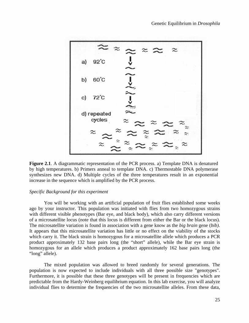
synthesize new DNA are added together in a tube to create a reaction mixture (primers, dNTPs, thermostable DNA polymerase, etc.). The tube is placed in a DNA thermal cycler which rapidly heats up and cools down, taking the reaction mixture through a series of temperature changes which occur as cycles. These cycles consist of three temperature stages which each accomplish different aspects of DNA amplification (See Figure 2.1; also, a helpful web site with a PCR animation can be found at: http://vector.cshl.org/Shockwave/pcranwhole.html). The first stage uses a high temperature (usually 92 or 94°C) which denatures the double stranded DNA into single strands. This step is necessary before new DNA can be synthesized on the single strands. The second stage uses a lower temperature at which the synthetic primers recognize, and form hydrogen bonds with their complementary sequence in the single stranded DNA (this is called annealing). The specific temperature of this stage depends on the base composition of the two primers. Specific annealing temperatures can be calculated for any given PCR primer. The third stage uses a temperature which is optimum for the function of the DNA polymerase which synthesizes the new DNA (usually 72°C). The thermal cycler takes the reaction mixture through many cycles (often as many as 35) of these three temperature stages, essentially doubling the sequence flanked by the primers with each cycle. This process results in an exponential increase in the number of copies of the sequence, so that millions of copies of the PCR product are present at the end of the process. This amplified DNA is so concentrated that it can be seen as a discrete band when the DNA is visualized on an electrophoresis gel. It is interesting to note that practical PCR was not possible until a thermostable DNA polymerase was isolated (one that would not be denatured by the 92-94°C DNA denaturation step). Such an enzyme (now called Taq polymerase) was first isolated from the bacterium Thermus aquaticus (= Taq) which thrives in hot springs where most living things cannot survive.


25

Figure 2.1. A diagrammatic representation of the PCR process. a) Template DNA is denatured by high temperatures. b) Primers anneal to template DNA. c) Thermostable DNA polymerase synthesizes new DNA. d) Multiple cycles of the three temperatures result in an exponential increase in the sequence which is amplified by the PCR process. Specific Background for this experiment You will be working with an artificial population of fruit flies established some weeks ago by your instructor. This population was initiated with flies from two homozygous strains with different visible phenotypes (Bar eye, and black body), which also carry different versions of a microsatellite locus (note that this locus is different from either the Bar or the black locus). The microsatellite variation is found in association with a gene know as the big brain gene (bib). It appears that this microsatellite variation has little or no effect on the viability of the stocks which carry it. The black strain is homozygous for a microsatellite allele which produces a PCR product approximately 132 base pairs long (the “short” allele), while the Bar eye strain is homozygous for an allele which produces a product approximately 162 base pairs long (the “long” allele). The mixed population was allowed to breed randomly for several generations. The population is now expected to include individuals with all three possible size "genotypes". Furthermore, it is possible that these three genotypes will be present in frequencies which are predictable from the Hardy-Weinberg equilibrium equation. In this lab exercise, you will analyze individual flies to determine the frequencies of the two microsatellite alleles. From these data,


26

you will then be able to determine if the genotype frequencies of this population are in Hardy-Weinberg equilibrium. Procedure This lab exercise will be conducted in four steps which include the following: 1) Grinding individual flies in a buffer solution, 2) Preparing and amplifying an individual PCR reaction for each fly to be tested, 3) Electrophoresis of PCR samples, and 4) Characterizing the bands present on the gels to determine the sizes and frequencies of the different bands. Steps 1 and 2 will be conducted during one lab period, and steps 3 and 4 will be conducted during the subsequent lab period. Instructions for each step of the experiment follow below. Step 1) Ginding individual flies in a buffer solution: a) Each student should isolate DNA and carry out PCR and electrophoresis for one or more

flies as instructed. Label one microcentrifuge tube for each fly with a code number as instructed. Place one anesthetized fly in each labeled tube. Several students should also process either a black or a Bar-eyed fly as a known “control” for later electrophoresis. Note the code number of the fly (flies) you are working with.

b) Add 50 µL of homogenization buffer to each tube and grind the fly with a plastic pestle.

Grind the fly as completely as possible. Use care when grinding. When removing the pestle, leave as much fly homogenate in the bottom of the tube as possible.

c) Incubate the tubes for 25 minutes at approximately 30°C. This can be accomplished by

placing the tubes in a floating tube “rack” in a 30°C water bath. d) Incubate the tubes for 1-2 minutes at about 95°C using a similar procedure. Use care when

removing the tubes from the hot water. e) If a microcentrifuge is available, briefly spin the homogenized flies so that remaining

tissues form a pellet at the bottom of the tube. Step 2) Preparing and amplifying an individual PCR reactions for each fly: a) Label a PCR tube for each homogenized fly using corresponding numbers. Transfer 2 µL

of Fly DNA solution into each labeled PCR tube. b) Add 23 µL of PCR “Master Mix”. The master mix contains all the components needed for

a PCR reaction except the Fly DNA (added in step a). The final PCR reaction contains the following: 10 mM Tris-HCl (pH 8.3), 0.75 Units of Taq polymerase, 50 mM KCl, 1.5 mM MgCl2, 0.2 mM dNTP mix, and 50 pmoles of each primer.

c) If your thermal cycler requires oil (your instructor will advise you of this), add 1-2 drops of

Rodney J. Scott, Genetic Equilibrium in Drosophila

27

mineral oil to the side of the PCR tube. It will form a layer over the aqueous PCR mixture. d) If you added oil, “pulse” spin PCR tubes in a microcentrifuge to separate completely the

aqueous PCR mix from the oil (CAUTION: Place PCR tubes within “larger” microcentrifuge tube WITH THE MICROCENTRIFUGE TUBE CAPS CUT OFF within the microcentrifuge - otherwise the PCR tubes will not remain in the rotor). Spin the tubes for several seconds.

e) Your instructor will set up the thermal cycler to conduct PCR, using the following cycling

conditions: Pre-amplification denaturing: one cycle of 2 minutes at 92°C. Amplification: 35 cycles of:

• 1 minute at 92°C. • 1 minute at 60°C. • 30 seconds at 72°C.

Note: For faster PCR or to allow for “hand cycling” (using two water baths for PCR instead of

a thermal cycler) the following two temperature/times may be substituted for the three temperature/times listed above: 94°C (or boiling) for 20 seconds, 70°C for 1 minute (repeat 29 times). The temperatures listed above (92, 60, and 72°C) were based on the original research report (Michalakis and Veuille, 1996), however, continued experimentation has shown that both the primer annealing step and the DNA synthesis step can be accomplished during one 70°C incubation time.

Post-amplification extension - 3 minutes at 72°C. Step 3) Electrophoresis of PCR samples: a) Add 5 µL of loading dye to the aqueous portion of each PCR sample. Burst spin as done in

step 2 to separate the oil from the dyed aqueous solution. b) Set your micropipette for the volume indicated by your instructor. Carefully submerge the

tip of your micropipette below the oil layer (if present) and slowly depress the plunger, expelling small air bubbles into the dyed aqueous solution. Then slowly release the plunger, aspirating the measured amount of the dyed PCR solution. Raise the tip above the oil layer and move the tip around the upper wall of the tube to remove excess oil adhering to the outside of the tip.

c) Add your sample to one well in the gel. Note which well(s) you load by submerging the tip

below the buffer solution directly into the opening of a well. Do not expel the solution until you are sure that the tip is inserted into a well, and do not insert the tip too far into the well


28

(be careful to avoid puncturing the bottom of the gel with your pipette tip). When you expel the sample into the well you should be able to see the colored solution settling into the well and filling it. One student should also load one lane on each gel with a molecular marker for size determination and another student should load a black or Bar-eyed control PCR product.

d) After the gel is loaded, your instructor will set the voltage. e) Allow the gel to run for approximately 1 hour. The gel should be viewed immediately

following electrophoresis. Step 4) Characterizing the bands present on the gels: View the gel(s) on an ultraviolet light box or use a gel documentation system to photograph the gel. If the gel is viewed directly (rather that viewing an image of the gel) wear appropriate plastic eye protection. Since prolonged exposure to UV light may also harm the skin, students may wish to wear a plastic face shield and appropriate clothing to cover exposed skin. The pattern in each sample lane should represent either a “long/long” homozygote (one band closer to the top of the gel), a “long/short” heterozygote (two bands), or a “short/short” homozygote (one band closer to the bottom of the gel). To verify that appropriate size bands were produced by PCR, you should compare the sample bands to the DNA in the molecular marker lane and also to the sample in the known control lane (from either a black, short/short fly, or a Bar-eyed, long/long fly). Depending on the efficiency of your DNA isolation technique, there may be one or more lighter bands in addition to the band(s) of expected size, however, in most cases, one or two bright bands should be obvious. To accomplish the analysis of the data from this experiment, the genotype (long/long, long/short, or short/short) of each sample must be determined and tabulated. You should do this in a large group with the assistance of your instructor. Each student will then analyze the entire data set according to the instructions below. Required Analysis

Answer the following questions and show your calculations as indicated. Question 1. How many flies of each genotype were present? long/long: long/short: short/short:


29

Question 2. What are the allele frequencies for each allele (long and short)? Show your calculations.

Question 3. Based on the Hardy-Weinberg theory, what are the expected frequencies of each

genotype? Show your calculations. Question 4. Do the observed genotypic frequencies fit the expected frequencies? Use a chi

square analysis to answer this question. Show your calculations and justify your answer by referring to the p value associated with the chi square value you estimate.

Note: The number of degrees of freedom for the analysis described above will not be 2 as you may expect, but rather, the d.f. in this case will equal 1. A different formula is used when comparing data to expected Hardy-Weinberg values than is the case when data are compared to expected Mendelian values. The general rule of thumb for Hardy-Weinberg analysis is that the number of degrees of freedom should equal the number of categories minus the number of alleles (in this case, d.f. = 3 - 2 = 1). This is true because the degrees of freedom should equal the number of classes minus the number of independent values obtained from the data that are used to determine the expected numbers. In the case of the Hardy-Weinberg analysis, two values must be estimated from the data - the number of individuals in each category, and the frequency of one of the alleles (Once the frequency for one allele has been calculated, the other can be determined by subtraction; i.e., if p is known, q = 1 - p). To assist you in analyzing your data based on Hardy-Weinberg equilibrium expectations, several example problems are given in the appendix of this exercise. Reference cited Michalakis, Y. and M. Veuille. 1996. Length variation of CAG/CAA trinucleotide repeats in

natural populations of Drosophila melanogaster and its relation to the recombinational rate. Genetics 143:1713-1725.

Appendix - Analyzing Populations for Hardy-Weinberg Equilibrium

The concepts associated with the Hardy-Weinberg theory can be very useful for making predictions about allele frequencies in a population. However, it is very important that you realize that some types of analyses are possible in some situations, but not possible in other situations. To complete the analysis of the data gained from the accompanying experiment, you will have to understand what type of calculations can be made from your data set. This appendix will present two different ways of analyzing population data. You should determine which example is most similar to your application and apply the corresponding analytical approach.


30

Estimating Genotype frequencies for Populations known to be in Equilibrium If a population is already known to be in Hardy-Weinberg Equilibrium, then it is possible to use the formula p2 + 2pq + q2 to estimate unknown genotype frequencies from known ones. For most genes, there are only two phenotypes (a dominant phenotype and a recessive one) but there are three genotypes. This means that in most cases the frequencies of two genotypes are unknown (i.e., AA and Aa), while the frequency of the third is known (i.e., aa; the frequency of this genotype will be the same as the frequency of the recessive phenotype). In such cases, the Hardy-Weinberg equation can be used to determine the frequency of the unknown genotypes if (and only if) one assumes that the population is in Hardy-Weinberg Equilibrium (under certain circumstances, this assumption can be justified, but not always). In the following example, this approach is used. Assume that a gene for a rare autosomal recessive phenotype is in Hardy-Weinberg Equilibrium. If 9 out of 10,000 individuals exhibit the recessive phenotype, how many may be expected to be heterozygous for this gene? If the population is in equilibrium (as the problem states), 9/10,000 should be equal to

q2 (the frequency of the recessive genotype). This means that q2 = 0.0009. From this, one may calculate q (the frequency of the recessive allele) as the square root of 0.0009, which equals 0.03.

If q = 0.03, p must be equal to 1 - q, or 1 - 0.03, which equals 0.97. If p = 0.97 and q = 0.03, the frequency of either of the unknown genotypes can be easily

calculated as follows: The frequency of the dominant homozygote equals p2 (which is 0.972), which equals 0.9409, or 94.09%.

The frequency of the heterozygote equals 2pq (which is 2(0.97)(0.03)), which equals 0.0582, or 5.82%.

Estimating Whether a Population is in Hardy-Weinberg Equilibrium based on Allele Frequencies If one knows allele frequencies for a population, but does not know whether that population is in equilibrium, the answer can be determined by a different strategy. In such cases, a four step strategy is used: 1) Determine the allele frequencies, 2) Predict the expected Hardy-Weinberg equilibrium genotype frequencies, 3) Compare the expected genotype frequencies to the observed ones, and 4) Interpret the analysis. Such an analysis is only useful when some way exists to determine actual genotype frequencies. In other words, this approach cannot be applied when it is only possible to tell the difference between organisms which exhibit one of two phenotypes (i.e., dominant or recessive).


31

For this reason, problems based on the MN blood group (a genetic system which exhibits codominance) are often used to demonstrate this approach. Students often think that this approach seems circular (using genotype frequencies to predict genotype frequencies and then comparing them), and they sometimes think that a “wrong answer” (“no equilibrium exists”) could not be generated by this approach. To demonstrate that this is not the case, two sets of population data will be analyzed below, one which fits Hardy-Weinberg equilibrium expectations (example A), and one which doesn’t (example B). Example A: 1,000 individuals from a human population are sampled for their MN blood group phenotypes/genotypes and the following data are reported: number of MM types: 642; number of MN types: 318; number of NN types: 40 Step 1) Determine the allele frequencies. There are several ways that this can be done, but the

following is perhaps the most obvious (and easy to remember).

There are 1,000 total individuals, therefore, there are 2,000 total M/N blood group alleles. Since homozygotes have two copies of their allele, these numbers must be doubled when considering allele frequencies. Since heterozygotes have only one copy of each allels, numbers of heterozygotes are used without doubling. The variables “p” and “q” can be assigned arbitrarily, since there is no dominant or recessive allele. In this example, p will equal the frequency of allele M. Allele frequencies are calculated as follows:

p = (2 x 642) + 318 = 0.801 q = (2 x 40) + 318 = 0.199 2000 2000 To double check your work, make sure that p + q = 1 (i.e., 0.801 + 0.199 = 1). Step 2) Predict the expected Hardy-Weinberg equilibrium genotype frequencies. This is done

simply by using the p and q values calculated above and the terms from the Hardy-Weinberg equation as follows:

Predicted frequency of MM = p2 = (0.801)2 = 0.6416 Predicted frequency of MN = 2pq = 2(0.801)(0.199) = 0.3188 Predicted frequency of NN = q2 = (0.199)2 = 0.0396 Step 3) Compare the expected genotype frequencies to the observed ones. This is done by

converting the predicted genotype frequencies into actual numbers and then comparing these to the observed numbers using a chi square analysis as follows:

Predicted number of MM = 0.6416 x 1000 = 641.6 Predicted number of MM = 0.3188 x 1000 = 318.8 Predicted number of MM = 0.0396 x 1000 = 39.6


32

(o-e)2 observed expected o-e expected 642 641.6 0.4 0.0002 318 318.8 -0.8 0.0020 40 39.6 0.4 0.0040 chi square = 0.0062 Step 4) Interpret the analysis. In this example, the interpretation is fairly obvious, the expected

numbers are obviously very close to the observed numbers. However, whether the comparison is obvious or not, the chi square value should be interpreted to support the conclusions (or to draw conclusions). This is done by consulting a chi square probability table and finding the associated p value. In this case, since there is one degrees of freedom (see the note following question 4 in the main section of the text for a discussion regarding determination of the degrees of freedom), when one consults the table, one finds that the p value is greater than 0.9. This is well beyond the generally accepted p value of 0.05, giving overwhelming support to our conclusion that the observed numbers do fit the expectations.

Example B: This is a similar example in which the numbers do not fit with Hardy-Weinberg expectations. The steps will be shown without the accompanying explanations given in Example A: 1,000 individuals from a human population are sampled for their MN blood group phenotypes/genotypes and the following data are reported: number of MM types: 500; number of MN types: 100; number of NN types: 400 Step 1) Determine the allele frequencies. p = (2 x 500) + 100 = 0.55 q = (2 x 400) + 100 = 0.45 2000 2000 p + q should still equal 1 (0.55 + 0.45 = 1) Step 2) Predict the expected Hardy-Weinberg equilibrium genotype frequencies. Predicted frequency of MM = p2 = (0.55)2 = 0.3025 Predicted frequency of MN = 2pq = 2(0.55)(0.45) = 0.495 Predicted frequency of NN = q2 = (0.45)2 = 0.2025


33

Step 3) Compare the expected genotype frequencies to the observed ones. Predicted number of MM = 0.3025 x 1000 = 302.5 Predicted number of MM = 0.495 x 1000 = 495 Predicted number of MM = 0.2025 x 1000 = 202.5 (o-e)2 observed expected o-e expected 500 302.5 197.5 128.9 100 495 -395 315.2 400 202.5 197.5 192.6 chi square = 636.7 Step 4) Interpret the analysis. Again, the numbers used in this example make the conclusion

fairly obvious - the predicted numbers don’t even come close to the observed numbers. However, again, this should be verified by using a p value table. When this is done, the chi square value calculated above is found to be vastly larger than the largest value considered to be acceptable (i.e., the largest acceptable value is 5.99 at the p = 0.05 level). Therefore, we can easily conclude that the observed genotypic frequencies are not in Hardy-Weinberg equilibrium (i.e., they do not match the expected frequencies closely enough).

Notes For the Instructor

Timing This lab activity requires several lab periods. The instructor may prepare the fly population ahead of time, or it is possible to have students do this (in either case, it is wise to prepare several populations in case one or more fail to thrive). There are four steps that students perform as described in the Student Outline. These steps include: 1) Grinding individual flies in a buffer solution to extract DNA, 2) Preparing PCR reactions for each fly to be tested, 3) Electrophoresis of PCR samples, and 4) Characterizing the bands present on the gels to determine the sizes and frequencies of the different bands. It is convenient to have students complete steps 1 and 2 in one lab period, run the PCR thermal cycler between labs, and then have students complete steps 3 and 4 in a final lab period. The work could be separated into three or four lab periods if necessary (each step could be done on a separate day). Also, if “hand cycling” is used to conduct PCR (using two water baths; see below), this will probably require an additional lab period. Fruit Fly Strains It is important to use flies which are known to carry the specific molecular markers described in this experiment. The experiment was developed using flies obtained from Carolina Biological Supply Company. The order numbers for these flies are as follows: Bar: BA-17-2110;


34

black: BA-17-2330. The Bar eye and black body flies were chosen after conducting analyses of many different strains. Bar and black were chosen not because of their physical phenotypes, but rather because of the fact that the PCR products (used as molecular markers in this experiment) were different enough in these strains to be distinguishable on agarose gels (instead of polyacrylamide gels, which are more difficult to use). Since highly inbred strains are used, the PCR products produced by flies of a given strain are all of equal (or nearly equal) length. DNA from different inbred strains of flies will produce PCR products of different sizes, and DNA from flies from natural populations will produce a variety of different sized PCR products. Such variations could be studied in other experiments, however, to obtain meaningful results in this experiment the fly strains listed above should be used.

Fruit Fly Cultures Flies may be grown under a variety of different conditions. It is convenient to use a commercial food mix such as Carolina’s “Formula 4-24". Adding yeast, as recommended by the makers of this mix seems to be unnecessary (and possibly even detrimental to the health of the culture), the flies seem to bring plenty of their own yeast into the cultures on their feet. It is convenient to grow the population cultures in large glass vessels (approximately 250 mL volume). The population culture must be initiated with a large number of healthy flies (see next paragraph). The population culture can be established with any proportion of Bar and black flies, however, it is wise not to use an extremely large number of one type and a small number of the other. If the numbers of flies in the initial population are too dissimilar, random chance (i.e., genetic drift) may result in the complete disappearance of one type (and possibly, the disappearance of one of the two molecular markers). Because fruit fly cultures can become infested with fungus (even if a fungal inhibitor is included in the medium), it is wise to take several precautions to ensure that a healthy population will be available to use for this experiment. Sometimes, cultures seem to become more easily infected if too few fruit flies are present initially (this may result because yeast grows more quickly than a small number of flies can consume it). Therefore, it is important to use a large number of flies to initiate the population. It is wise to set up several large bottles, each containing a large total number of flies (around 150 or more), and then use the most healthy culture as the population culture. The female flies do not need to be virgin flies (as in Mendelian crosses), since mating will be random in subsequent generations. In order for Hardy-Weinberg equilibrium to become established in a population culture, the flies should be allowed to interbreed for approximately 6-8 weeks prior to sampling. Since the establishment of Hardy-Weinberg equilibrium requires very large numbers of individuals, it is unlikely that samples taken prior to 6-8 weeks will exhibit equilibrium. The requirement for large numbers of randomly interbreeding individuals also means that one should not expect the allele frequencies of the sample taken at 6-8 weeks to be based on the initial allele frequencies in the founder population. Because the founding population will be small (relative to Hardy-


35

Weinberg conditions), the first several generations will be expected to vary somewhat randomly with regard to allele frequencies. Of course, if one is interested in having a class study the population over time (instead of just taking one sample), it would be very interesting to take several samples and see how long it actually takes for equilibrium to be established. Sampling the Population After a fly population has grown for 6-8 weeks or more, it is difficult to remove living flies directly from the container because so many dead flies are present. To get around this problem, it is helpful to attach a smaller “sampling vial” (with food mix at the bottom) to the mouth of the larger population bottle and allow the population flies to lay eggs in this smaller vial. It is good to use a small bottle with a neck that can be inserted into the mouth of the larger bottle and then wrap tape around the juncture of the two bottles (to prevent emigration). The smaller bottle can be left in place until larvae are visible to ensure that a good sample can be obtained. Homogenizing Flies and Extracting DNA The flies are ground in 50 µL of Extraction Buffer (See recipe in the Appendix) in a microcentrifuge tube. This buffer and the extraction protocol given in the Student Outline, are based on the protocol given by Gloor et al., (1993). There are many possible ways that flies can be homogenized, two methods have been used successfully by the author. Small plastic pestles with matched tubes which can be obtained from Bioworld (catalogue number: 008-705; www.bio-world.com) work quite nicely. It is also possible to buy the pestles separately, however, one must ensure that they fit one’s microcentrifuge tubes snugly (some tubes are too narrow at the bottom). It is also possible to use the disposable plastic tip of a micropipette to homogenize a fly adequately. If this technique is used, students should dispense a “drop” of the extraction buffer, homogenize the fly, and then add the remaining volume of extraction buffer.

Either technique produces a mixture of solution and fly parts. Students should continue grinding their flies until there are no recognizable body parts visible. It is very important to emphasize to students that they need to grind carefully, so that their homogenate doesn’t “disappear” (i.e., it may dry up on the sides of the tube). After grinding, there are several additional steps which release the DNA, and destroy DNA-degrading compounds (see Student Outline). There is some flexibility regarding the times and temperatures listed in the outline. The incubation which is described as being “25 minutes at about 30°C” can be anywhere from 20 to 30 minutes long, and the temperature can range from about 25 - 37°C. Also, the incubation which is described as being “1-2 minutes at about 95°C” can be accomplished in much warmer water (possibly even boiling). The final “extract” will appear very impure, but as long as the students add mostly solution to their PCR reactions (rather than fly parts), this generally works as a DNA source.


36

Preparing PCR Reactions It is convenient to use a PCR mix sold by Sigma chemical company called “ReadyMix Taq PCR Reaction Mix” (catalogue number: P 4600). It comes in a 2X concentrated form, and the instructions recommend using 25 µL to prepare 50 µL reactions. It is possible to use 12.5 µL per reaction to make 25 µL reactions, and it is such reactions which are used in this exercise. The “Readymix” solution can be stored for long periods of time if stored according to accompanying instructions. Other types of PCR mixtures may work equally well, however they should be pre-tested to ensure that similar results will be obtained (significant variations do exist). The Student Outline refers to the use of a “Master Mix” (which contains everything but DNA). This mixture is prepared as follows. For each 25 µL reaction, prepare 23 µL worth of “Master Mix”. For each reaction, use 12.5 µL of ReadyMix, 9.5 µL of high grade dH2O, and 0.5 µL of each primer (2 primers x 0.5 µL = 1.0 µL). Students then add 2.0 µL of DNA solution and 23 µL of master mix to each PCR tube as described in the Student Outline. This solution should be mixed by aspiration with a micropipettor. If one uses a PCR thermal cycler which has a heated lid, it will be unnecessary to add oil. Otherwise, students should add a drop of mineral oil as described in the student outline. Mineral oil should also be added if the PCR reactions will be “hand cycled” (See notes under the heading PCR conditions).

The final concentration of the various components in the 25 µL reactions is as follows: 10 mM Tris-HCl (pH 8.3), 0.75 Units of Taq polymerase, 50 mM KCl, 1.5 mM MgCl2, 0.2 mM dNTP mix, and 0.5 µL of each primer (100 pmoles/µL for each primer). Information for Synthesis and Handling of PCR Primers The sequences for the primers were described by Michalakis and Veuille (1996) . The PCR primers have the following sequences: GREG-5-P: (5'-3') TCGCAAGGATCAGCGGTGAC GREG-5-M: (5'-3') TTGGGCCTCAGCGGCAGCAT PCR primers can be ordered from many companies for approximately $1.00 per base (or less). The amounts that are provided will be enough for many experiments and can last when stored at -20 for many months (years?). The author orders primers from “Alpha DNA” (http://www.alphadna.com/) . At the time these notes were written, their price for primers was $0.48 per base, with no additional set up cost. This company sends the primers as lyophilized samples in small, plastic tubes. Each sample comes with a print-out containing details regarding the synthesis of the sample. Included in these details is an estimate of the amount of sample provided, given in Picomoles. It is convenient to


37

use this information to calculate how much TE buffer (See recipe in the Appendix) to add in order to prepare the primers at a concentration of 100 pmole per primer. One may simply divide the number of pmoles indicated by 100 and add that amount of TE buffer. After adding TE buffer the mixture should be repeatedly aspirated with a micropipettor to dissolve the lyophilized primer completely. PCR Conditions: The PCR reaction described in the Student Outline has been routinely run using the following PCR cycle conditions: Pre-amplification denaturing - one cycle of 2 minutes at 92°C. Amplification: 35 cycles of:

• 1 minute at 92°C (Denaturation) • 1 minute at 60°C (Annealing) • 30 sec. at 72°C (Extension)

Post-amplification extension: 3 minutes at 72°C. However, recent, continued experimentation has shown that is possible to replace the 60 degree annealing temperature with a 70 degree temperature. This modification makes it possible to combine the annealing step (60°C above) and the extension step (72°C above) into one step at 70°C. This change can be used to reduce the overall time necessary to conduct PCR with a thermal cycler, and also makes it possible to conduct “hand cycling”, using two water baths instead of a PCR thermal cycler. If this modification is used, the following PCR protocol can be employed (with a thermal cycler or with two water baths):

Pre-amplification denaturing - omit this step (if boiling water is used, periods of longer than 20 seconds may denature the polymerase) .

Amplification: 30 cycles of:

• 20 seconds at 94°C (or use boiling water) (Denaturation) Note: Do not incubate for longer than 20 seconds.

• 1 minute at 70°C (Annealing and Extension)

Post-amplification extension. This step may be omitted. Note: The rationale for using the modified PCR protocol should be clearly explained to students. This is why the original, three step protocol has been left in the Student Outline. It should be emphasized to students that although the annealing step and the extension step are being


38

combined together in one temperature-step, both molecular events are still occurring at this one temperature. PCR products can be stored at 4°C for several weeks or more. It should also be possible to store them for prolonged periods at - 20 (in a non-defrosting freezer). Preparing and Running Gels Gels are made with a 0.5X TBE buffer (See recipe in the Appendix), with 3% “Super Fine Resolution” agarose (cat. number J234-100G, made by Amresco. This can be ordered from Midwest Scientific, http://www.midsci.com/). The agarose mixture is prepared in a microwave oven. It is allowed to cool slightly, and then ethidium bromide (EtBr) (to stain the DNA) is added directly to the agarose mixture. 2.86 µL of a 10 mg/mL EtBr solution should be added per 100 mL of agarose mixture. It is also possible to run gels without EtBr in the gel and then later soak them in an EtBr solution, but this is less convenient and more dangerous (EtBr is a potent mutagen). The amount of agarose mixture needed will vary depending on the size of the gel trays being used. Note: Since EtBr is a potent mutagen it should be handled with care. Use gloves whenever working with EtBr and ensure that any items containing EtBr are properly disposed of according to your institution’s guidelines. The tank buffer is exactly the same 0.5X TBE buffer as that used for the gel. The PCR samples are loaded in the gel by mixing them with a 6X loading buffer (See recipe in the Appendix). This gives the samples a blue color and also makes them denser than the tank buffer so they can be loaded while the gel is submerged. Samples are prepared using 5 parts PCR product to 1 part 6X loading buffer. The amount of sample you will need to add to each well will be determined by the size of gel comb you use (to form the wells) and the thickness of the gels you pour (wells typically hold volumes in the range of 10-20 µL) . A DNA size marker should be added to at least one well on each gel. One such marker which works well for this experiment is called “PCR DNA marker” (cat. number: E854, made by Amresco, and available from Midwest Scientific, http://www.midsci.com/). Use a mixture of 5 parts “PCR DNA marker” to 5 parts dH2O to 2 parts 6X loading buffer (See recipe in the Appendix) to prepare the size marker for electrophoresis. Run the gel at about 120-130 volts for about 1.5 to 2 hours. If a lower voltage is used it will take longer to run the gel. A higher voltage will produce aberrations in the bands on the gel.


39

Characterization of the Gels: Gels are placed on a ultraviolet transilluminator which causes the EtBr-stained DNA to fluoresce. Neither the illuminated gel, nor the UV light source should be directly viewed with the naked eye. The illuminated gel can be photographed, or viewed through a protective plastic shield. Note: Since UV light is mutagenic, students should be warned about this danger if gels are to be viewed directly (versus using a camera). Damage to the eye is probably the greatest danger. However, UV light may also cause damage to the skin. Therefore students should be given the option of wearing a full face protective shield and a lab coat if gels are to be viewed directly. The two main PCR products are approximately 132 and 162 base pairs long. These products will be located in the gel near the second smallest DNA fragment in the size marker lane if “PCR DNA marker” is used (the three smallest fragments in this marker are 50, 150, and 300 base pairs long). Three different PCR “genotypes” should be evident among the flies from the population (162/162, 162/132, and 132/132). These should be present in frequencies which fit the Hardy-Weinberg ratio (See the Appendix of the Student Outline for details). As with any other kind of data set, the more individuals that are sampled, the better the fit which is likely to occur between observed and expected numbers. However, a meaningful chi square analysis can be conducted on a relatively small sample. In this case, the expected numbers in each class should be at least 5. If the expected number in one class is less than 5, Yates’s correction should be applied. A complete description of these considerations can be found in Modern Genetics, by F.J. Ayala and J.A. Kiger, Jr. (Benjamin/Cummings Publishing, 1980) in that text’s Appendix II. Note that the number of degrees of freedom for a chi square analysis of these data will not be 2 (as one might expect, based on the familiar d.f. = n - 1) but rather, the d.f. in this case will equal 1. A different formula is used when comparing data to expected Hardy-Weinberg values than is the case when data are compared to expected Mendelian values. The general rule of thumb for Hardy-Weinberg analysis is that the number of degrees of freedom should equal the number of categories minus the number of alleles (in this case, d.f. = 3 - 2 = 1). This is true because the degrees of freedom should equal the number of classes minus the number of independent values obtained from the data that are used to determine the expected numbers. In the case of the Hardy-Weinberg analysis, two values must be estimated from the data - the number of individuals in each category, and the frequency of one of the alleles (once the frequency for one allele has been calculated, the other can be determined by subtraction; i.e., if p is known, q = 1 - p). This topic is also comprehensively covered in the text by Ayala and Kiger (1980)


40

Acknowledgments

I thank the administrators of Wheaton College for providing me with the time and resources to pursue the research which enabled me to develop this laboratory exercise. I also thank my colleagues in the Biology Department for their support and encouragement. I thank student John C. Reece, who dedicated much time and effort to helping me work out the details of this laboratory activity. And finally, I thank the students in my classes whose enthusiasm inspires my work.

Literature Cited Ayala, F. J., and J. A. Kiger Jr., 1980. Appendix II. Pages 788-790, in Modern Genetics. The

Benjamin/Cummings Publishing Company, Inc., 844 pages. [ISBN 0-8053-0312-X] Gloor, G. B., C. R. Preston, D. M. Johnson-Schlitz, N. A. Nassif, R. W. Phillis, W. K. Benz, H.

M. Robertson and W. R. Engels. 1993. Type I repressors of P element mobility. Genetics 135:81-95.

Michalakis, Y. and M. Veuille. 1996. Length variation of CAG/CAA trinucleotide repeats in

natural populations of Drosophila melanogaster and its relation to the recombinational rate. Genetics 143:1713-1725.


41

Appendix Recipes for Solutions “Homogenization Buffer”: 10 mM Tris-HCl (pH 8.2) 1 mM EDTA (Use EDTA disodium salt, dihydrate and adjust pH with NaOH.) 25 mM NaCl 200 µg/mL Proteinase K This Homogenization Buffer may be stored for one year or longer at - 20°C (in a non-defrosting freezer). TE (Tris-EDTA) Buffer (pH = 7.0): For a 500 mL solution: 5 mL 1 M Tris (pH = 7.0; Use Tris base and adjust pH with concentrated HCl) 1 mL 0.5 M EDTA (pH = 7.0) (Use EDTA disodium salt, dihydrate and adjust pH with NaOH.) Bring the solution to a final volume of 500 mL with dH2O. Autoclave. If TE is kept sterile, it may be stored at room temperature. 5X TBE buffer stock (this is 10X the concentration used for gels and tank buffer): 54.0 g Tris Base 27.5 g Boric Acid 3.72 g Na2EDTA.2H2O Bring to a final volume of 1 liter with dH20. Mix to dissolve. TBE buffer can be stored at room temperature. If a precipitate forms after long term storage of the 5X stock, it should be remade. 6X Gel loading buffer: 4 g Sucrose 25 mg Bromophenol Blue Dye 2.4 mL 0.5 M EDTA, pH 8.0 (Use EDTA disodium salt, dihydrate and adjust pH with NaOH.) Bring to a final volume of 10 mL with dH2O 6X loading buffer can be stored for short periods at 4°C and for longer periods at - 20°C. Information about Suppliers Carolina Biological Supply Company Fruit Flies: Bar - catalogue number BA-17-2110; black - catalogue number BA-17-2330. Formula 4-24: catalogue number BA-17-3200. Several kits containing components necessary for conducting this experiment can now be


42

obtained from Carolina Biological Supply Company as follows: Drosophila PCR amplification kit: catalogue number 21-1240; Drosophila PCR amplification and electrophoresis kit (with ethidium bromide): catalogue number 21-1242; Drosophila PCR amplification and electrophoresis kit (with CarolinaBLU stain): catalogue number 21-1244; Drosophila PCR amplification replacement kit: catalogue number 21-1246. Phone: 1-800-334-5551 Web Site: http://www.carolina.com/ Bioworld Pestels and matched centrifuge tubes: catalogue number 008-705. Phone: 1-800-860-9729 Web Site: www.bio-world.com Sigma Chemical Company ReadyMix Taq PCR Reaction Mix: catalogue number P 4600. Phone: 1-800-325-3010 Web Site: http://www.sigma-aldrich.com/ Alpha DNA Primers can be custom ordered from their web site Phone: 1-800-511-3654 Web Site: http://www.alphadna.com/ Midwest Scientific Super Fine Resolution Agar: catalogue number J234-100G. PCR DNA marker: catalogue number E854. Phone: 1-800-227-9997 Web Site: http://www.midsci.com/

using a molecular marker to study genetic equilibrium in ... · laboratory manual (2001) morton...

Documents