u.s.fish&wildlifeservice adaptiveharvest management
TRANSCRIPT

U.S. Fish & Wildlife Service
Adaptive HarvestManagement2021 Hunting Season

Adaptive Harvest Management2021 Hunting Season
PREFACE
The process of setting waterfowl hunting regulations is conducted annually in the United States (U.S.; Blohm1989) and involves a number of meetings where the status of waterfowl is reviewed by the agencies responsiblefor setting hunting regulations. In addition, the U.S. Fish and Wildlife Service (USFWS) publishes proposedregulations in the Federal Register to allow public comment. This document is part of a series of reportsintended to support development of harvest regulations for the 2021 hunting season. Specifically, this reportis intended to provide waterfowl managers and the public with information about the use of adaptive harvestmanagement (AHM) for setting waterfowl hunting regulations in the U.S. This report provides the mostcurrent data, analyses, and decision-making protocols. However, adaptive management is a dynamic processand some information presented in this report will differ from that in previous reports.
Citation: U.S. Fish and Wildlife Service. 2020. Adaptive Harvest Management: 2021 Hunting Season.U.S. Department of Interior, Washington, D.C. 109 pp. Available online at http://www.fws.gov/birds/
management/adaptive-harvest-management/publications-and-reports.php
ACKNOWLEDGMENTS
A Harvest Management Working Group (HMWG) comprised of representatives from the USFWS, the U.S.Geological Survey (USGS), the Canadian Wildlife Service (CWS), and the four Flyway Councils (Appendix A)was established in 1992 to review the scientific basis for managing waterfowl harvests. The working group,supported by technical experts from the waterfowl management and research communities, subsequentlyproposed a framework for adaptive harvest management, which was first implemented in 1995. The USFWSexpresses its gratitude to the HMWG and to the many other individuals, organizations, and agencies thathave contributed to the development and implementation of AHM.
We are grateful for the continuing technical support from our USGS colleagues: F. A. Johnson (Retired),M. C. Runge, and J. A. Royle. We are also grateful to K. Pardieck, J. Sauer, K. Brantley, J. Byun, N.Hanke, M. Lutmerding, D. Murry, and D. Ziolkowski of the USGS Patuxent Wildlife Research Center, andthe thousands of USGS Breeding Bird Survey participants for providing wood duck data in a timely manner.We acknowledge that information provided by USGS in this report has not received the Director’s approvaland, as such, is provisional and subject to revision. In addition, we acknowledge that the use of trade, firm,or product names does not imply endorsement by these agencies.
This report was prepared by the USFWS Division of Migratory Bird Management. G. S. Boomer and G.S. Zimmerman were the principal authors. Individuals that provided essential information or otherwiseassisted with report preparation included: J. Hostetler, P. Devers, N. Zimpfer, K. Fleming, and R. Raftovich(USFWS). Comments regarding this document should be sent to the Chief, Division of Migratory BirdManagement, U.S. Fish & Wildlife Service Headquarters, MS: MB, 5275 Leesburg Pike, Falls Church, VA22041-3803.
Cover art: The 2020–2021 Federal Duck Stamp featuring black-bellied whistling-ducks (Dendrocygna au-tumnalis) painted by Eddie LeRoy.
2

TABLE OF CONTENTS1 EXECUTIVE SUMMARY 7
2 BACKGROUND 9
3 ADJUSTMENTS TO THE 2020 REGULATORY PROCESS 10
4 WATERFOWL STOCKS AND FLYWAY MANAGEMENT 10
5 WATERFOWL POPULATION DYNAMICS 125.1 Mid-Continent Mallard Stock . . . . . . . . . . . . . . . . . . . . . . . . . . . . . . . . . . . . 125.2 Western Mallard Stock . . . . . . . . . . . . . . . . . . . . . . . . . . . . . . . . . . . . . . . . 135.3 Atlantic Flyway Multi-Stock . . . . . . . . . . . . . . . . . . . . . . . . . . . . . . . . . . . . . 14
6 HARVEST-MANAGEMENT OBJECTIVES 16
7 REGULATORY ALTERNATIVES 167.1 Evolution of Alternatives . . . . . . . . . . . . . . . . . . . . . . . . . . . . . . . . . . . . . . 167.2 Regulation-Specific Harvest Rates . . . . . . . . . . . . . . . . . . . . . . . . . . . . . . . . . 17
8 OPTIMAL REGULATORY STRATEGIES 20
9 APPLICATION OF ADAPTIVE HARVEST MANAGEMENT CONCEPTS TO OTHERSTOCKS 259.1 American Black Duck . . . . . . . . . . . . . . . . . . . . . . . . . . . . . . . . . . . . . . . . 259.2 Northern Pintails . . . . . . . . . . . . . . . . . . . . . . . . . . . . . . . . . . . . . . . . . . . 299.3 Scaup . . . . . . . . . . . . . . . . . . . . . . . . . . . . . . . . . . . . . . . . . . . . . . . . . 33
10 EMERGING ISSUES IN ADAPTIVE HARVEST MANAGEMENT 34
LITERATURE CITED 36
Appendix A Harvest Management Working Group Members 40
Appendix B 2021-2022 Regulatory Schedule 43
Appendix C Proposed Fiscal Year 2021 Harvest Management Working Group Priorities 44
Appendix D 2020 Canadian Pond Forecast 45
Appendix E 2020 Great Lakes Mallard Population Forecast 56
Appendix F 2020 Eastern Mallard Population Forecast 65
Appendix G 2020 Pintail Breeding Population Distribution (Latitude) Forecast 72
Appendix H Mid-Continent Mallard Models 81
Appendix I Western Mallard Models 85
Appendix J Atlantic Flyway Multi-stock Models 91
Appendix K Modeling Waterfowl Harvest Rates 95
Appendix L Northern Pintail Models 101
Appendix M Scaup Model 106
3

LIST OF FIGURES1 Waterfowl Breeding Population and Habitat Survey (WBPHS) strata and state, provincial, and
territorial survey areas currently assigned to the mid-continent and western stocks of mallardsand eastern waterfowl stocks for the purposes of adaptive harvest management. . . . . . . . . 11
2 Population estimates of mid-continent mallards observed in the WBPHS (strata: 13–18, 20–50,and 75–77) and the Great Lakes region (Michigan, Minnesota, and Wisconsin) from 1992 to2019. . . . . . . . . . . . . . . . . . . . . . . . . . . . . . . . . . . . . . . . . . . . . . . . . . . 12
3 Top panel: population estimates of mid-continent mallards observed in the WBPHS comparedto mid-continent mallard model set predictions (weighted average based on 2019 model weightupdates) from 1996 to 2019. Bottom panel: mid-continent mallard model weights. . . . . . . 13
4 Population estimates of western mallards observed in Alaska (WBPHS strata 1–12) and thesouthern Pacific Flyway (California, Oregon, Washington, and British Columbia combined)from 1990 to 2019. . . . . . . . . . . . . . . . . . . . . . . . . . . . . . . . . . . . . . . . . . . 14
5 Population estimates of American green-winged teal (AGWT), wood ducks (WODU), ring-necked ducks (RNDU), and goldeneyes (GOLD) observed in eastern Canada (WBPHS strata51–53, 56, 62–72) and U.S. (Atlantic Flyway states) from 1998 to 2019. . . . . . . . . . . . . 15
6 Mid-continent mallard pre-survey harvest policies derived with updated optimization methodsthat account for changes in decision timing associated with adaptive harvest managementprotocols specified in the SEIS 2013. . . . . . . . . . . . . . . . . . . . . . . . . . . . . . . . . 22
7 Western mallard pre-survey harvest policies derived with updated optimization methods thataccount for changes in decision timing associated with adaptive harvest management protocolsspecified under the SEIS 2013. . . . . . . . . . . . . . . . . . . . . . . . . . . . . . . . . . . . 22
8 Atlantic Flyway multi-stock pre-survey harvest policies derived with updated optimizationmethods that account for changes in decision timing associated with adaptive harvest man-agement protocols specified under the SEIS 2013. . . . . . . . . . . . . . . . . . . . . . . . . . 25
9 Functional form of the harvest parity constraint designed to allocate allowable black duckharvest equally between the U.S. and Canada. . . . . . . . . . . . . . . . . . . . . . . . . . . 27
10 Predictive harvest rate distributions for adult male black ducks expected under the applicationof the current regulatory alternatives in Canada (left) and the U.S. (right). . . . . . . . . . . 28
11 Updated median estimates of black duck harvest additivity (a1 ; top panel) and mallard com-petition (c2 ; bottom panel) parameters over time. . . . . . . . . . . . . . . . . . . . . . . . . 29
12 Northern pintail pre-survey harvest policies derived with updated optimization methods thataccount for changes in decision timing associated with adaptive harvest management protocolsspecified in the SEIS 2013. . . . . . . . . . . . . . . . . . . . . . . . . . . . . . . . . . . . . . . 32
B.1 Schedule of biological information availability, regulation meetings, and Federal Register pub-lications for the 2021–2022 hunting season. . . . . . . . . . . . . . . . . . . . . . . . . . . . . 43
L.1 Harvest yield curves resulting from an equilibrium analysis of the northern pintail model setbased on 2019 model weights. . . . . . . . . . . . . . . . . . . . . . . . . . . . . . . . . . . . . 105
4

LIST OF TABLES1 Current regulatory alternatives for the duck-hunting season. . . . . . . . . . . . . . . . . . . . 182 Predictions of harvest rates of adult male, mid-continent and western mallards expected with
application of the current regulatory alternatives in the Mississippi, Central and Pacific Flyways. 193 Predictions of harvest rates of American green-winged teal (AGWT), wood ducks (WODU),
ring-necked ducks (RNDU), and goldeneyes (GOLD) expected under closed, restrictive, mod-erate, and liberal regulations in the Atlantic Flyway. . . . . . . . . . . . . . . . . . . . . . . . 20
4 Optimal regulatory strategy for the Mississippi and Central Flyways for the 2021 hunting season. 235 Optimal regulatory strategy for the Pacific Flyway for the 2021 hunting season. . . . . . . . . 246 Optimal regulatory strategy for the Atlantic Flyway for the 2021 hunting season. . . . . . . . 267 Black duck optimal regulatory strategies for Canada and the United States for the 2021 hunting
season. . . . . . . . . . . . . . . . . . . . . . . . . . . . . . . . . . . . . . . . . . . . . . . . . . 308 Substitution rules in the Central and Mississippi Flyways for joint implementation of northern
pintail and mallard harvest strategies. . . . . . . . . . . . . . . . . . . . . . . . . . . . . . . . 319 Northern pintail optimal regulatory strategy for the 2021 hunting season. . . . . . . . . . . . 3210 Regulatory alternatives and total expected harvest levels corresponding to the closed, restric-
tive, moderate, and liberal packages considered in the scaup adaptive harvest managementdecision framework. . . . . . . . . . . . . . . . . . . . . . . . . . . . . . . . . . . . . . . . . . 33
11 Scaup optimal regulatory strategy for the 2021 hunting season. . . . . . . . . . . . . . . . . . 35C.1 Priority rankings and project leads identified for the technical work proposed at the 2019
Harvest Management Working Group meeting and updated during the summer of 2020. . . . 44H.1 Estimates (N) and associated standard errors (SE) of mid-continent mallards (in millions) ob-
served in the WBPHS (strata 13–18, 20–50, and 75–77) and the Great Lakes region (Michigan,Minnesota, and Wisconsin) from 1992 to 2019. . . . . . . . . . . . . . . . . . . . . . . . . . . 81
I.1 Estimates (N) and associated standard errors (SE) of western mallards (in millions) observedin Alaska ( WBPHS strata 1–12) and the southern Pacific Flyway (California, Oregon, Wash-ington, and British Columbia combined) from 1990 to 2019. . . . . . . . . . . . . . . . . . . . 85
I.2 Estimates of model parameters resulting from fitting a discrete logistic model to a time seriesof estimated population sizes and harvest rates of mallards breeding in Alaska from 1990 to2019. . . . . . . . . . . . . . . . . . . . . . . . . . . . . . . . . . . . . . . . . . . . . . . . . . . 89
I.3 Estimates of model parameters resulting from fitting a discrete logistic model to a time seriesof estimated population sizes and harvest rates of mallards breeding in the southern PacificFlyway (California, Oregon, Washington, and British Columbia combined) from 1992 to 2019. 90
J.1 Estimates (N) and associated standard errors (SE) of American green-winged teal (AGWT),wood ducks (WODU), ring-necked ducks (RNDU), and goldeneyes (GOLD) (in millions) ob-served in eastern Canada (WBPHS strata 51–53, 56, 62–72) and U.S. (Atlantic Flyway states)from 1998 to 2019. . . . . . . . . . . . . . . . . . . . . . . . . . . . . . . . . . . . . . . . . . . 91
J.2 Estimates of model parameters resulting from fitting a discrete logistic model to a time seriesof estimated population sizes and harvest rates of American green-winged teal (AGWT), woodducks (WODU), ring-necked ducks (RNDU), and goldeneyes (GOLD) breeding in easternCanada and U.S. from 1998 to 2019. . . . . . . . . . . . . . . . . . . . . . . . . . . . . . . . . 93
J.3 Lognormal mean and standard deviations (SD) used to describe the prior distributions formaximum intrinsic growth rate (r) for American green-winged teal (AGWT), wood ducks(WODU), ring-necked ducks (RNDU), and goldeneyes (GOLD) in eastern Canada and U.S. . 94
K.1 Parameter estimates for predicting mid-continent mallard harvest rates resulting from a hier-archical, Bayesian analysis of mid-continent mallard band-recovery information from 1998 to2019. . . . . . . . . . . . . . . . . . . . . . . . . . . . . . . . . . . . . . . . . . . . . . . . . . . 97
K.2 Parameter estimates for predicting western mallard harvest rates resulting from a hierarchical,Bayesian analysis of western mallard band-recovery information from 2008 to 2019. . . . . . . 98
K.3 Annual harvest rate estimates (h) and associated standard errors (SE) for American green-winged teal (AGWT), wood ducks (WODU), ring-necked ducks (RNDU), and goldeneyes(GOLD) in eastern Canada (WBPHS strata 51–53, 56, 62–72) and U.S. (Atlantic Flywaystates) from 1998 to 2019. . . . . . . . . . . . . . . . . . . . . . . . . . . . . . . . . . . . . . . 99
5
K.4 Parameter estimates for predicting American green-winged teal (AGWT), wood duck (WODU),ring-necked duck (RNDU), and goldeneye (GOLD) expected harvest rates for season lengths< 60 days and bag limits < 6 birds. . . . . . . . . . . . . . . . . . . . . . . . . . . . . . . . . . 100
L.1 Total pintail harvest expected from the set of regulatory alternatives specified for each Flywayunder the northern pintail adaptive harvest management protocol. . . . . . . . . . . . . . . . 103
M.1 Model parameter estimates resulting from a Bayesian analysis of scaup breeding population,harvest, and banding information from 1974 to 2019. . . . . . . . . . . . . . . . . . . . . . . . 109
6
1 EXECUTIVE SUMMARY
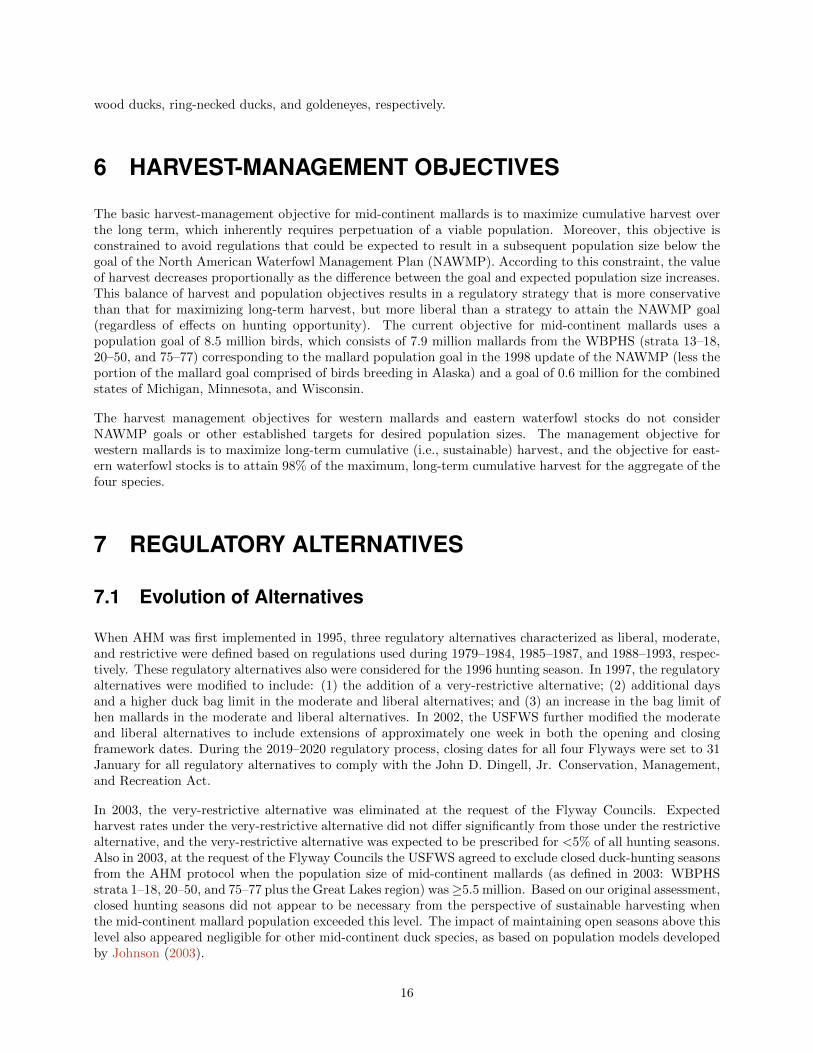
In 1995 the U.S. Fish and Wildlife Service (USFWS) implemented the adaptive harvest management (AHM)program for setting duck hunting regulations in the United States (U.S.). The AHM approach provides aframework for making objective decisions in the face of incomplete knowledge concerning waterfowl populationdynamics and regulatory impacts.
The coronavirus disease 2019 (COVID-19) pandemic prevented the USFWS and their partners from perform-ing the Waterfowl Breeding Population and Habitat Survey (WBPHS) and estimating waterfowl breedingpopulations and habitat conditions in the spring of 2020. As a result, AHM protocols have been adjustedto inform duck hunting regulations based on model predictions of breeding populations and habitat condi-tions. In most cases, system models specific to each AHM decision framework have been used to predictbreeding population sizes from the available information (e.g., 2019 observations). However, for some systemstate variables we have used updated time series models to forecast 2020 values based on the most recentinformation.
The AHM protocol is based on the population dynamics and status of two mallard (Anas platyrhynchos)stocks and a suite of waterfowl stocks in the Atlantic Flyway. Mid-continent mallards are defined as thosebreeding in the WBPHS strata 13–18, 20–50, and 75–77 plus mallards breeding in the states of Michigan,Minnesota, and Wisconsin (state surveys). The prescribed regulatory alternative for the Mississippi andCentral Flyways depends exclusively on the status of these mallards. Western mallards are defined as thosebreeding in WBPHS strata 1–12 (hereafter Alaska) and in the states of California, Oregon, Washington, andthe Canadian province of British Columbia (hereafter southern Pacific Flyway). The prescribed regulatoryalternative for the Pacific Flyway depends exclusively on the status of these mallards. In 2018, the AtlanticFlyway and the USFWS adopted a multi-stock AHM protocol based on 4 populations of eastern waterfowl[American green-winged teal (Anas crecca), wood ducks (Aix sponsa), ring-necked ducks (Aythya collaris),and goldeneyes (both Bucephala clangula and B. islandica combined)]. The regulatory choice for the AtlanticFlyway depends exclusively on the status of these waterfowl populations.
Mallard population models are based on the best available information and account for uncertainty in popula-tion dynamics and the impact of harvest. Model-specific weights reflect the relative confidence in alternativehypotheses and are updated annually using comparisons of predicted to observed population sizes. Formid-continent mallards, current model weights favor the weakly density-dependent reproductive hypothesis(>99%) and the additive-mortality hypothesis (72%). Unlike mid-continent mallards, we consider a singlefunctional form to predict western mallard and eastern waterfowl population dynamics but consider a widerange of parameter values each weighted relative to the support from the data.
For the 2021 hunting season, the USFWS is considering similar regulatory alternatives as 2020. The nature ofthe restrictive, moderate, and liberal alternatives has remained essentially unchanged since 1997, except thatextended framework dates have been offered in the moderate and liberal alternatives since 2002. Harvestrates associated with each of the regulatory alternatives have been updated based on band-recovery datafrom pre-season banded birds. The expected harvest rates of adult males under liberal hunting seasons are0.11, and 0.13 for mid-continent and western mallards, respectively. In the Atlantic Flyway, expected harvestrates under the liberal alternative are 0.12, 0.12, 0.13, and 0.03 for American green-winged teal, wood ducks,ring-necked ducks, and goldeneyes, respectively.
Optimal regulatory strategies for the 2021 hunting season were calculated using: (1) harvest-managementobjectives specific to each stock; (2) current regulatory alternatives; and (3) current population modelsand their relative weights. Based on liberal regulatory alternatives selected for the 2020 hunting season, a2020 prediction of 9.07 million mid-continent mallards, 3.40 million ponds in Prairie Canada, 0.94 millionwestern mallards predicted for Alaska (0.41 million) and the southern Pacific Flyway (0.53 million), and 0.35million American green-winged teal, 0.94 million wood ducks, 0.70 million ring-necked ducks and 0.58 milliongoldeneyes predicted for the eastern survey area and Atlantic Flyway, the optimal choice for the 2021 huntingseason in all four Flyways is the liberal regulatory alternative.
7

AHM concepts and tools have been successfully applied toward the development of formal adaptive harvestmanagement protocols that inform American black duck (Anas rubripes), northern pintail (Anas acuta), andscaup (Aythya affinis, A. marila combined) harvest decisions.
For black ducks, the optimal country-specific regulatory strategies for the 2021 hunting season were calculatedusing: (1) an objective to achieve 98% of the maximum, long-term cumulative harvest; (2) current country-specific black duck regulatory alternatives; and (3) updated model parameters and weights. Based on a liberalregulatory alternative selected by Canada and a moderate regulatory alternative selected by the U.S. for the2020 hunting season and the 2020 model prediction of 0.50 million breeding black ducks and 0.39 millionbreeding mallards predicted for the core survey area, the optimal regulatory choices for the 2021 huntingseason are the liberal regulatory alternative in Canada and the moderate regulatory alternative in the UnitedStates.
For pintails, the optimal regulatory strategy for the 2021 hunting season was calculated using: (1) an objectiveof maximizing long-term cumulative harvest; (2) current pintail regulatory alternatives; and (3) currentpopulation models and their relative weights. Based on a liberal regulatory alternative with a 1-bird dailybag limit selected for the 2020 hunting season and the 2020 model prediction of 2.446 million pintails predictedto settle at a mean latitude of 55.16 degrees, the optimal regulatory choice for the 2021 hunting season forall four Flyways is the liberal regulatory alternative with a 1-bird daily bag limit.
For scaup, the optimal regulatory strategy for the 2021 hunting season was calculated using: (1) an objectiveto achieve 95% of the maximum, long-term cumulative harvest; (2) current scaup regulatory alternatives;and (3) updated model parameters and weights. Based on a restrictive regulatory alternative selected for the2020 hunting season and a 2020 model prediction of 3.53 million scaup, the optimal regulatory choice for the2021 hunting season for all four Flyways is the restrictive regulatory alternative.
8

2 BACKGROUND
The annual process of setting duck-hunting regulations in the U.S. is based on a system of resource monitor-ing, data analyses, and rule-making (Blohm 1989). Each year, monitoring activities such as aerial surveys,preseason banding, and hunter questionnaires provide information on population size, habitat conditions,and harvest levels. Data collected from these monitoring programs are analyzed each year, and proposals forduck-hunting regulations are developed by the Flyway Councils, States, and USFWS. After extensive publicreview, the USFWS announces regulatory guidelines within which States can set their hunting seasons.
In 1995, the USFWS adopted the concept of adaptive resource management (Walters 1986) for regulatingduck harvests in the U.S. This approach explicitly recognizes that the consequences of hunting regulationscannot be predicted with certainty and provides a framework for making objective decisions in the face ofthat uncertainty (Williams and Johnson 1995). Inherent in the adaptive approach is an awareness thatmanagement performance can be maximized only if regulatory effects can be predicted reliably. Thus, adap-tive management relies on an iterative cycle of monitoring, assessment, and decision-making to clarify therelationships among hunting regulations, harvests, and waterfowl abundance (Johnson et al. 2016).
In regulating waterfowl harvests, managers face four fundamental sources of uncertainty (Nichols et al. 1995a,Johnson et al. 1996, Williams et al. 1996):
(1) environmental variation – the temporal and spatial variation in weather conditions and other keyfeatures of waterfowl habitat; an example is the annual change in the number of ponds in the PrairiePothole Region, where water conditions influence duck reproductive success;
(2) partial controllability – the ability of managers to control harvest only within limits; the harvest resultingfrom a particular set of hunting regulations cannot be predicted with certainty because of variation inweather conditions, timing of migration, hunter effort, and other factors;
(3) partial observability – the ability to estimate key population attributes (e.g., population size, reproduc-tive rate, harvest) only within the precision afforded by extant monitoring programs; and
(4) structural uncertainty – an incomplete understanding of biological processes; a familiar example isthe long-standing debate about whether harvest is additive to other sources of mortality or whetherpopulations compensate for hunting losses through reduced natural mortality. Structural uncertaintyincreases contentiousness in the decision-making process and decreases the extent to which managerscan meet long-term conservation goals.
AHM was developed as a systematic process for dealing objectively with these uncertainties. The key com-ponents of AHM include (Johnson et al. 1993, Williams and Johnson 1995):
(1) a limited number of regulatory alternatives, which describe Flyway-specific season lengths, bag limits,and framework dates;
(2) a set of population models describing various hypotheses about the effects of harvest and environmentalfactors on waterfowl abundance;
(3) a measure of reliability (probability or “weight”) for each population model; and
(4) a mathematical description of the objective(s) of harvest management (i.e., an “objective function”),by which alternative regulatory strategies can be compared.
These components are used in a stochastic optimization procedure to derive a regulatory strategy. A regula-tory strategy specifies the optimal regulatory choice, with respect to the stated management objectives, foreach possible combination of breeding population size, environmental conditions, and model weights (Johnsonet al. 1997). The setting of annual hunting regulations then involves an iterative process:
9

(1) each year, an optimal regulatory choice is identified based on resource and environmental conditions,and on current model weights;
(2) after the regulatory decision is made, model-specific predictions for subsequent breeding population sizeare determined;
(3) when monitoring data become available, model weights are increased to the extent that observations ofpopulation size agree with predictions, and decreased to the extent that they disagree; and
(4) the new model weights are used to start another iteration of the process.
By iteratively updating model weights and optimizing regulatory choices, the process should eventuallyidentify which model is the best overall predictor of changes in population abundance. The process is optimalin the sense that it provides the regulatory choice each year necessary to maximize management performance.It is adaptive in the sense that the harvest strategy “evolves” to account for new knowledge generated by acomparison of predicted and observed population sizes.
3 ADJUSTMENTS TO THE 2020 REGULATORY PROCESS
Due to the coronavirus disease 2019 (COVID-19) pandemic, the USFWS and their partners were unableto perform the WBPHS and estimate waterfowl breeding populations as well as evaluate breeding habitatconditions in the spring of 2020. As a result, the information requirements, assessment methodologies,and decision protocols that typically define the annual regulatory process have required some modifications.The lack of an observable population size has immediate implications for learning through AHM. Modelpredictions for 2020 population responses cannot be compared to WBPHS estimates to update model weights.Because of this lack of updating, the USFWS and the Flyway councils have agreed to use optimal harvestpolicies calculated with model weights and model parameters based on the most recent information availableto inform waterfowl harvest decisions for the 2020 regulations process. These policies represent optimaldecisions based on our most recent observations and understanding of system dynamics. In the absence of2020 breeding population information, the USFWS and Flyway councils have agreed to use predictions ofbreeding population sizes and habitat conditions to determine regulatory decisions for the 2021-22 huntingseason. Current system models for which we have AHM decision frameworks were used to predict 2020population sizes as a function of breeding population sizes, habitat conditions, harvest, and harvest ratesobserved during the 2019–20 hunting seasons. For some state variables (e.g., Canadian ponds) or 2019unobservable information (e.g., Canadian harvest), we used formal time series analyses methods (Hyndmanand Athanasopoulos 2018) to forecast these values. We provide the results of these forecasts in the body ofthis report and include the analytical details in the attached appendices.
4 WATERFOWL STOCKS AND FLYWAY MANAGEMENT
Since its inception AHM has focused on the population dynamics and harvest potential of mallards, especiallythose breeding in mid-continent North America. Mallards constitute a large portion of the total U.S. duckharvest, and traditionally have been a reliable indicator of the status of many other species. Geographicdifferences in the reproduction, mortality, and migrations of waterfowl stocks suggest that there may becorresponding differences in optimal levels of sport harvest. The ability to regulate harvests of mallardsoriginating from various breeding areas is complicated, however, by the fact that a large degree of mixingoccurs during the hunting season. The challenge for managers, then, is to vary hunting regulations amongFlyways in a manner that recognizes each Flyway’s unique breeding-ground derivation of waterfowl stocks.Of course, no Flyway receives waterfowl exclusively from one breeding area; therefore, Flyway-specific harveststrategies ideally should account for multiple breeding stocks that are exposed to a common harvest.
10

Figure 1 – Waterfowl Breeding Population and Habitat Survey (WBPHS) strata and state, provincial, andterritorial survey areas currently assigned to the mid-continent and western stocks of mallards and easternwaterfowl stocks for the purposes of adaptive harvest management.
The optimization procedures used in AHM can account for breeding populations of waterfowl beyond themid-continent region, and for the manner in which these ducks distribute themselves among the Flywaysduring the hunting season. An optimal approach would allow for Flyway-specific regulatory strategies, whichrepresent an average of the optimal harvest strategies for each contributing breeding stock weighted by therelative size of each stock in the fall flight. This joint optimization of multiple stocks requires: (1) models ofpopulation dynamics for all recognized stocks; (2) an objective function that accounts for harvest-managementgoals for all stocks in the aggregate; and (3) decision rules allowing Flyway-specific regulatory choices. Atpresent, however, a joint optimization of western, mid-continent, and eastern stocks is not feasible due tocomputational hurdles. However, our preliminary analyses suggest that the lack of a joint optimization doesnot result in a significant decrease in management performance.
Currently, two stocks of mallards (mid-continent and western) and stocks of four different species of easternwaterfowl populations (Atlantic Flyway multi-stock; hereafter ’multi-stock’) are recognized for the purposesof AHM (Figure 1). We use a constrained approach to the optimization of these stocks’ harvest, in whichthe regulatory strategy for the Mississippi and Central Flyways is based exclusively on the status of mid-continent mallards and the Pacific Flyway regulatory strategy is based exclusively on the status of westernmallards. Historically, the Atlantic Flyway regulatory strategy was based exclusively on the status of easternmallards. In 2018, the Atlantic Flyway and the USFWS adopted a multi-stock AHM framework. As a result,the Atlantic Flyway regulatory strategy is based exclusively on the status of American green-winged teal,wood ducks, ring-necked ducks, and goldeneyes breeding in the Atlantic Flyway states and eastern Canada.
11

46
810
12
Year
TotalWBPHS
Pop
ulat
ion
Siz
e (m
illio
ns)
1995 2000 2005 2010 2015 2020
0.6
0.8
1.0
1.2
YearYear
Great Lakes
Figure 2 – Population estimates of mid-continent mallards observed in the WBPHS (strata: 13–18, 20–50,and 75–77) and the Great Lakes region (Michigan, Minnesota, and Wisconsin) from 1992 to 2019. Error barsrepresent one standard error. The 2020 values are based on model predictions.
5 WATERFOWL POPULATION DYNAMICS
5.1 Mid-Continent Mallard Stock
Mid-continent mallards are defined as those breeding in WBPHS strata 13–18, 20–50, and 75–77, and inthe Great Lakes region (Michigan, Minnesota, and Wisconsin; see Figure 1). Estimates of this populationhave varied from 6.3 to 11.9 million since 1992 (Table H.1, Figure 2). For 2020, we used each model in themid-continent mallard model set to predict the 2020 breeding population size and used the updated 2019model weights to calculate a weighted average breeding population size of 8.34 million (SE = 1.43 million).In addition, we used a formal time series analysis to forecast a 2020 breeding population of Great Lakesregion mallards equal to 0.73 million (SE = 0.12 million), see Appendix (D) for details. The total 2020mid-continent mallard breeding population is predicted to be 9.07 million (SE = 1.43 million).
Details describing the set of population models for mid-continent mallards are provided in Appendix H. Theset consists of four alternatives, formed by the combination of two survival hypotheses (additive vs. compen-satory hunting mortality) and two reproductive hypotheses (strongly vs. weakly density dependent). Relativeweights for the alternative models of mid-continent mallards changed little until all models under-predictedthe change in population size from 1998 to 1999, perhaps indicating there is a significant factor affectingpopulation dynamics that is absent from all four models (Figure 3). Updated model weights suggest greaterevidence for the additive-mortality models (72%) over those describing hunting mortality as compensatory(28%). For most of the time frame, model weights have strongly favored the weakly density-dependent re-productive models over the strongly density-dependent ones, with current model weights greater than 99%and less than 1%, respectively. The reader is cautioned, however, that models can sometimes make reliablepredictions of population size for reasons having little to do with the biological hypotheses expressed therein(Johnson et al. 2002).
12

67
89
1012
Year
Pop
ulat
ion
Siz
e (m
illio
ns)
ObservedPredicted
1995 2000 2005 2010 2015 2020
0.0
0.2
0.4
0.6
Year
Mod
el W
eigh
ts
SaRwScRwSaRsScRs
Year
Figure 3 – Top panel: population estimates of mid-continent mallards observed in the WBPHS compared tomid-continent mallard model set predictions (weighted average based on 2019 model weight updates) from 1996to 2019. Error bars represent 95% confidence intervals. Bottom panel: mid-continent mallard model weights(SaRw = additive mortality and weakly density-dependent reproduction, ScRw = compensatory mortality andweakly density-dependent reproduction, SaRs = additive mortality and strongly density-dependent reproduction,ScRs = compensatory mortality and strongly density-dependent reproduction). Model weights were assumed tobe equal in 1995 and model weight updates were not calculated for 2020.
5.2 Western Mallard Stock
Western mallards consist of 2 substocks and are defined as those birds breeding in Alaska (WBPHS strata1–12) and those birds breeding in the southern Pacific Flyway (California, Oregon, Washington, and BritishColumbia combined; see Figure 1). Estimates of these subpopulations have varied from 0.28 to 0.84 millionin Alaska since 1990 and 0.43 to 0.64 million in the southern Pacific Flyway since 2010 (Table I.1, Figure 4).For 2020, we used the western mallard models and Bayesian estimation frameworks to predict a medianbreeding-population size of 0.94 million (SE = 0.09 million), including 0.41 million (SE = 0.07 million) fromAlaska and 0.53 million (SE = 0.06 million) from the southern Pacific Flyway.
Details concerning the set of population models for western mallards are provided in Appendix I. To predictchanges in abundance we used a discrete logistic model, which combines reproduction and natural mortalityinto a single parameter, r, the intrinsic rate of growth. This model assumes density-dependent growth,which is regulated by the ratio of population size, N, to the carrying capacity of the environment, K (i.e.,equilibrium population size in the absence of harvest). In the traditional formulation of the logistic model,harvest mortality is completely additive and any compensation for hunting losses occurs as a result of density-dependent responses beginning in the subsequent breeding season. To increase the model’s generality weincluded a scaling parameter for harvest that allows for the possibility of compensation prior to the breedingseason. It is important to note, however, that this parameterization does not incorporate any hypothesizedmechanism for harvest compensation and, therefore, must be interpreted cautiously. We modeled Alaskamallards independently of those in the southern Pacific Flyway because of differing population trajectories(see Figure 4) and substantial differences in the distribution of band recoveries.
We used Bayesian estimation methods in combination with a state-space model that accounts explicitly forboth process and observation error in breeding population size (Meyer and Millar 1999). Breeding populationestimates of mallards in Alaska are available since 1955, but we had to limit the time series to 1990–2019because of changes in survey methodology and insufficient band-recovery data. The logistic model and
13

0.0
0.5
1.0
1.5
Year
Western Mallard TotalAlaska
1990 1995 2000 2005 2010 2015 2020
0.0
0.2
0.4
0.6
0.8
1.0
Year
Southern PF TotalCA−ORWA−BC
Pop
ulat
ion
Siz
e (m
illio
ns)
Figure 4 – Population estimates of western mallards observed in Alaska (WBPHS strata 1–12) and the southernPacific Flyway (California, Oregon, Washington, and British Columbia combined) from 1990 to 2019. Error barsrepresent one standard error. The 2020 values are based on model predictions.
associated posterior parameter estimates provided a reasonable fit to the observed time series of Alaskapopulation estimates. The estimated median carrying capacity was 1.02 million and the intrinsic rate ofgrowth was 0.28. The posterior median estimate of the scaling parameter was 1.35. Breeding populationand harvest-rate data were available for California-Oregon mallards for the period 1992–2019. Because theBritish Columbia survey did not begin until 2006 and the Washington survey was redesigned in 2010, weimputed data in a Markov chain Monte Carlo (MCMC) framework from the beginning of the British Columbiaand Washington surveys back to 1992 (see details in Appendix I) to make the time series consistent for thesouthern Pacific Flyway. The logistic model also provided a reasonable fit to these data. The estimatedmedian carrying capacity was 0.79 million, and the intrinsic rate of growth was 0.25. The posterior medianestimate of the scaling parameter was 0.46.
The AHM protocol for western mallards is structured similarly to that used for mid-continent mallards, inwhich an optimal harvest strategy is based on the status of a single breeding stock (Alaska and southernPacific Flyway substocks) and harvest regulations in a single Flyway. Although the contribution of mid-continent mallards to the Pacific Flyway harvest is significant, we believe an independent harvest strategyfor western mallards poses little risk to the mid-continent stock. Further analyses will be needed to confirmthis conclusion, and to better understand the potential effect of mid-continent mallard status on sustainablehunting opportunities in the Pacific Flyway.
5.3 Atlantic Flyway Multi-Stock
For the purposes of the Atlantic Flyway multi-stock AHM framework, eastern waterfowl stocks are definedas those breeding in eastern Canada and Maine (USFWS fixed-wing surveys in WBPHS strata 51-53, 56,and 62-70; CWS helicopter plot surveys in WBPHS strata 51-52, 63-64, 66-68, and 70-72) and AtlanticFlyway states from New Hampshire south to Virginia (AFBWS; Heusmann and Sauer 2000). These areas
14

0.5
1.0
1.5
Year
WODURNDU
2000 2005 2010 2015 2020
0.2
0.4
0.6
0.8
1.0
1.2
1998:endyr
e.bp
op$A
GW
T.N
AGWTGOLD
Pop
ulat
ion
Siz
e (m
illio
ns)
Figure 5 – Population estimates of American green-winged teal (AGWT), wood ducks (WODU), ring-neckedducks (RNDU), and goldeneyes (GOLD) observed in eastern Canada (WBPHS strata 51–53, 56, 62–72) and U.S.(Atlantic Flyway states) from 1998 to 2019. Error bars represent one standard error. The SE of the goldeneyesestimate for 2013 is not reported due to insufficient counts. The 2020 values are based on model predictions.
have been consistently surveyed since 1998. Breeding population size estimates for American green-wingedteal, ring-necked ducks, and goldeneyes are derived annually by integrating USFWS and CWS survey datafrom eastern Canada and Maine (WBPHS strata 51-53, 56, and 62-72; (Zimmerman et al. 2012, U.S. Fishand Wildlife Service 2019b). Insufficient counts of American green-winged teal, ring-necked ducks, andgoldeneyes in the AFBWS preclude the inclusion of those areas in the population estimates for those species.Breeding population size estimates for wood ducks in the Atlantic Flyway (Maine south to Florida) areestimated by integrating data from the AFBWS and the Breeding Bird Survey (BBS; Zimmerman et al.2015). Insufficient counts of wood ducks from the USFWS and CWS surveys in Maine and Canada precludeincorporating those survey results into breeding population estimates. Estimates of the breeding populationsize for American green-winged teal have varied from 0.30 to 0.46 million, wood ducks varied from 0.92 to1.04 million, ring-necked ducks varied from 0.59 to 0.92 million, and goldeneyes varied from 0.44 to 0.85million since 1998 (Table J.1, Figure 5). For 2020, we used the multi-stock population models and Bayesianestimation frameworks to predict a median breeding population size of 0.35 million (SE = 0.04 million) forAmerican green-winged teal, 0.94 million (SE = 0.07 million) for wood ducks, 0.70 million (SE = 0.07 million)for ring-necked ducks, and 0.58 million (SE = 0.10 million) for goldeneyes.
Details concerning the set of models used in Atlantic Flyway multi-stock AHM are provided in Appendix J.Similar to the methods used in western mallard AHM, we used a discrete logistic model to represent easternwaterfowl population and harvest dynamics and a state-space, Bayesian estimation framework to estimatethe population parameters and process variation. We modeled each stock independently and found that thelogistic model and associated posterior parameter estimates provided a reasonable fit to the observed timeseries of eastern waterfowl stocks. The estimated median carrying capacities were 0.53, 1.56, 0.87, and 0.71for American green-winged teal, wood ducks, ring-necked ducks, and goldeneyes, respectively. The posteriormedian estimates of intrinsic rate of growth were 0.43, 0.39, 0.40, and 0.23 for American green-winged teal,
15
wood ducks, ring-necked ducks, and goldeneyes, respectively.
6 HARVEST-MANAGEMENT OBJECTIVES
The basic harvest-management objective for mid-continent mallards is to maximize cumulative harvest overthe long term, which inherently requires perpetuation of a viable population. Moreover, this objective isconstrained to avoid regulations that could be expected to result in a subsequent population size below thegoal of the North American Waterfowl Management Plan (NAWMP). According to this constraint, the valueof harvest decreases proportionally as the difference between the goal and expected population size increases.This balance of harvest and population objectives results in a regulatory strategy that is more conservativethan that for maximizing long-term harvest, but more liberal than a strategy to attain the NAWMP goal(regardless of effects on hunting opportunity). The current objective for mid-continent mallards uses apopulation goal of 8.5 million birds, which consists of 7.9 million mallards from the WBPHS (strata 13–18,20–50, and 75–77) corresponding to the mallard population goal in the 1998 update of the NAWMP (less theportion of the mallard goal comprised of birds breeding in Alaska) and a goal of 0.6 million for the combinedstates of Michigan, Minnesota, and Wisconsin.
The harvest management objectives for western mallards and eastern waterfowl stocks do not considerNAWMP goals or other established targets for desired population sizes. The management objective forwestern mallards is to maximize long-term cumulative (i.e., sustainable) harvest, and the objective for east-ern waterfowl stocks is to attain 98% of the maximum, long-term cumulative harvest for the aggregate of thefour species.
7 REGULATORY ALTERNATIVES
7.1 Evolution of Alternatives
When AHM was first implemented in 1995, three regulatory alternatives characterized as liberal, moderate,and restrictive were defined based on regulations used during 1979–1984, 1985–1987, and 1988–1993, respec-tively. These regulatory alternatives also were considered for the 1996 hunting season. In 1997, the regulatoryalternatives were modified to include: (1) the addition of a very-restrictive alternative; (2) additional daysand a higher duck bag limit in the moderate and liberal alternatives; and (3) an increase in the bag limit ofhen mallards in the moderate and liberal alternatives. In 2002, the USFWS further modified the moderateand liberal alternatives to include extensions of approximately one week in both the opening and closingframework dates. During the 2019–2020 regulatory process, closing dates for all four Flyways were set to 31January for all regulatory alternatives to comply with the John D. Dingell, Jr. Conservation, Management,and Recreation Act.
In 2003, the very-restrictive alternative was eliminated at the request of the Flyway Councils. Expectedharvest rates under the very-restrictive alternative did not differ significantly from those under the restrictivealternative, and the very-restrictive alternative was expected to be prescribed for <5% of all hunting seasons.Also in 2003, at the request of the Flyway Councils the USFWS agreed to exclude closed duck-hunting seasonsfrom the AHM protocol when the population size of mid-continent mallards (as defined in 2003: WBPHSstrata 1–18, 20–50, and 75–77 plus the Great Lakes region) was≥5.5 million. Based on our original assessment,closed hunting seasons did not appear to be necessary from the perspective of sustainable harvesting whenthe mid-continent mallard population exceeded this level. The impact of maintaining open seasons above thislevel also appeared negligible for other mid-continent duck species, as based on population models developedby Johnson (2003).
16

In 2008, the mid-continent mallard stock was redefined to exclude mallards breeding in Alaska, necessitatinga re-scaling of the closed-season constraint. Initially, we attempted to adjust the original 5.5 million closurethreshold by subtracting out the 1985 Alaska breeding population estimate, which was the year upon whichthe original closed season constraint was based. Our initial re-scaling resulted in a new threshold equal to5.25 million. Simulations based on optimal policies using this revised closed season constraint suggested thatthe Mississippi and Central Flyways would experience a 70% increase in the frequency of closed seasons. Atthat time, we agreed to consider alternative re-scalings in order to minimize the effects on the mid-continentmallard strategy and account for the increase in mean breeding population sizes in Alaska over the pastseveral decades. Based on this assessment, we recommended a revised closed season constraint of 4.75 millionwhich resulted in a strategy performance equivalent to the performance expected prior to the re-definition ofthe mid-continent mallard stock. Because the performance of the revised strategy is essentially unchangedfrom the original strategy, we believe it will have no greater impact on other duck stocks in the Mississippiand Central Flyways. However, complete- or partial-season closures for particular species or populationscould still be deemed necessary in some situations regardless of the status of mid-continent mallards.
For the development of the multi-stock AHM framework in the Atlantic Flyway, the USFWS and Atlantic Fly-way decided to keep the same overall bag limits and season lengths that were used for eastern mallard AHM.Species-specific regulations are then based on harvest strategies informed by existing decision frameworks(e.g., black duck AHM).
At the time this report was prepared, the regulatory packages for the 2021-22 seasons had not been finalizedby the U.S. Fish and Wildlife Service. However, we do not expect any changes from the 2020-21 packages.Therefore, optimal strategies were formulated using the 2020-21 packages and are referred to as “current”packages in subsequent text. Details of the regulatory alternatives for each Flyway are provided in Table 1.
7.2 Regulation-Specific Harvest Rates
Harvest rates of mallards associated with each of the open-season regulatory alternatives were initially pre-dicted using harvest-rate estimates from 1979–1984, which were adjusted to reflect current hunter numbersand contemporary specifications of season lengths and bag limits. In the case of closed seasons in the UnitedStates, we assumed rates of harvest would be similar to those observed in Canada during 1988–1993, whichwas a period of restrictive regulations both in Canada and the United States. All harvest-rate predictionswere based only in part on band-recovery data, and relied heavily on models of hunting effort and successderived from hunter surveys (Appendix C in U.S. Fish and Wildlife Service 2002). As such, these predictionshad large sampling variances and their accuracy was uncertain.
In 2002, we began using Bayesian statistical methods for improving regulation-specific predictions of harvestrates, including predictions of the effects of framework-date extensions. Essentially, the idea is to use existing(prior) information to develop initial harvest-rate predictions (as above), to make regulatory decisions basedon those predictions, and then to observe realized harvest rates. Those observed harvest rates, in turn, aretreated as new sources of information for calculating updated (posterior) predictions. Bayesian methods areattractive because they provide a quantitative, formal, and an intuitive approach to adaptive management.
Annual harvest rate estimates for mid-continent and western mallards and eastern stocks of American green-winged teal and wood ducks are updated with band-recovery information from a cooperative banding programbetween the USFWS and CWS, along with state, provincial, and other participating partners. Recovery rateestimates from these data are adjusted with reporting rate probabilities resulting from recent reward bandstudies (Boomer et al. 2013, Garrettson et al. 2013). For mid-continent mallards, we have empirical estimatesof harvest rate from the recent period of liberal hunting regulations (1998–2019). Bayesian methods allow usto combine these estimates with our prior predictions to provide updated estimates of harvest rates expectedunder the liberal regulatory alternative. Moreover, in the absence of experience (so far) with the restrictiveand moderate regulatory alternatives, we reasoned that our initial predictions of harvest rates associated withthose alternatives should be re-scaled based on a comparison of predicted and observed harvest rates underthe liberal regulatory alternative. In other words, if observed harvest rates under the liberal alternative were
17
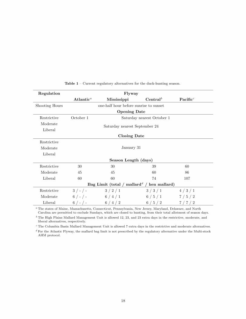
Table 1 – Current regulatory alternatives for the duck-hunting season.
Regulation Flyway
Atlantica Mississippi Centralb Pacificc
Shooting Hours one-half hour before sunrise to sunset
Opening Date
Restrictive October 1 Saturday nearest October 1
ModerateSaturday nearest September 24
Liberal
Closing Date
Restrictive
Moderate January 31
Liberal
Season Length (days)
Restrictive 30 30 39 60
Moderate 45 45 60 86
Liberal 60 60 74 107
Bag Limit (total / mallardd / hen mallard)
Restrictive 3 / - / - 3 / 2 / 1 3 / 3 / 1 4 / 3 / 1
Moderate 6 / - / - 6 / 4 / 1 6 / 5 / 1 7 / 5 / 2
Liberal 6 / - / - 6 / 4 / 2 6 / 5 / 2 7 / 7 / 2a The states of Maine, Massachusetts, Connecticut, Pennsylvania, New Jersey, Maryland, Delaware, and NorthCarolina are permitted to exclude Sundays, which are closed to hunting, from their total allotment of season days.
b The High Plains Mallard Management Unit is allowed 12, 23, and 23 extra days in the restrictive, moderate, andliberal alternatives, respectively.
c The Columbia Basin Mallard Management Unit is allowed 7 extra days in the restrictive and moderate alternatives.d For the Atlantic Flyway, the mallard bag limit is not prescribed by the regulatory alternative under the Multi-stockAHM protocol.
18

10% less than predicted, then we might also expect that the mean harvest rate under the moderate alternativewould be 10% less than predicted. The appropriate scaling factors currently are based exclusively on priorbeliefs about differences in mean harvest rate among regulatory alternatives, but they will be updated oncewe have experience with something other than the liberal alternative. A detailed description of the analyticalframework for modeling mallard harvest rates is provided in Appendix K.
Our models of regulation-specific harvest rates also allow for the marginal effect of framework-date extensionsin the moderate and liberal alternatives. A previous analysis by the U.S. Fish and Wildlife Service (2001)suggested that implementation of framework-date extensions might be expected to increase the harvest rate ofmid-continent mallards by about 15%, or in absolute terms by about 0.02 (SD = 0.01). Based on the observedharvest rates during the 2002–2019 hunting seasons, the updated (posterior) estimate of the marginal changein harvest rate attributable to the framework-date extension is 0.004 (SD = 0.006). The estimated effect ofthe framework-date extension has been to increase harvest rate of mid-continent mallards by about 3% overwhat would otherwise be expected in the liberal alternative. However, the reader is strongly cautioned thatreliable inference about the marginal effect of framework-date extensions ultimately depends on a rigorousexperimental design (including controls and random application of treatments).
Current predictions of harvest rates of adult-male mid-continent mallards associated with each of the regu-latory alternatives are provided in Table 2. Predictions of harvest rates for the other age and sex cohorts arebased on the historical ratios of cohort-specific harvest rates to adult-male rates (Runge et al. 2002). Theseratios are considered fixed at their long-term averages and are 1.5407, 0.7191, and 1.1175 for young males,adult females, and young females, respectively. We make the simplifying assumption that the harvest ratesof mid-continent mallards depend solely on the regulatory choice in the Mississippi and Central Flyways.
Based on available estimates of harvest rates of mallards banded in California and Oregon during 1990–1995and 2002–2007, there was no apparent relationship between harvest rate and regulatory changes in the PacificFlyway. This is unusual given our ability to document such a relationship in other mallard stocks and in otherspecies. We note, however, that the period 2002–2007 was comprised of both stable and liberal regulationsand harvest rate estimates were based solely on reward bands. Regulations were relatively restrictive duringmost of the earlier period and harvest rates were estimated based on standard bands using reporting ratesestimated from reward banding during 1987–1988. Additionally, 1993–1995 were transition years in whichfull-address and toll-free bands were being introduced and information to assess their reporting rates (andtheir effects on reporting rates of standard bands) is limited. Thus, the two periods in which we wish tocompare harvest rates are characterized not only by changes in regulations, but also in estimation methods.
Consequently, we lack a sound empirical basis for predicting harvest rates of western mallards associatedwith current regulatory alternatives other than liberal in the Pacific Flyway. In 2009, we began usingBayesian statistical methods for improving regulation-specific predictions of harvest rates (see Appendix K).The methodology is analogous to that currently in use for mid-continent mallards except that the marginaleffect of framework date extensions in moderate and liberal alternatives is inestimable because there are nodata prior to implementation of extensions. In 2008, we specified prior regulation-specific harvest rates of0.01, 0.06, 0.09, and 0.11 with associated standard deviations of 0.003, 0.02, 0.03, and 0.03 for the closed,
Table 2 – Predictions of harvest rates of adult male, mid-continent and western mallards expected with appli-cation of the current regulatory alternatives in the Mississippi, Central and Pacific Flyways.
Mid-continent Western
Regulatory Alternative Mean SD Mean SD
Closed (U.S.) 0.009 0.002 0.009 0.018
Restrictive 0.054 0.013 0.069 0.017
Moderate 0.094 0.021 0.115 0.029
Liberal 0.111 0.017 0.135 0.027
19

restrictive, moderate, and liberal alternatives, respectively. The prior for the liberal regulation was thenupdated in 2011 with a harvest rate of 0.12 and standard deviation of 0.04. The harvest rates for the liberalalternative were based on empirical estimates realized under the current liberal alternative during 2002–2007 and determined from adult male mallards banded with reward and standard bands adjusted for bandreporting rates in the southern Pacific Flyway. The development of priors was based on banding informationfrom California and Oregon data only. Recently, we assessed the band-recovery data from Washington, Idaho,and British Columbia and found that the addition of these bands had a negligible influence on harvest rateestimates of western mallards. As a result, we have included Washington, Idaho, and British Columbia band-recovery information in our annual updates to western mallard harvest rate distributions. Harvest rates forthe moderate and restrictive alternatives were based on the proportional (0.85 and 0.51) difference in harvestrates expected for mid-continent mallards under the respective alternatives. Finally, harvest rate for theclosed alternative was based on what we might realize with a closed season in the United States (includingAlaska) and a very restrictive season in Canada, similar to that for mid-continent mallards. A relativelylarge standard deviation (CV = 0.3) was chosen to reflect greater uncertainty about the means than thatfor mid-continent mallards (CV = 0.2). Current predictions of harvest rates of adult male western mallardsassociated with each regulatory alternative are provided in Table 2.
The harvest rates expected under the liberal season for the four populations associated with the AtlanticFlyway’s multi-stock AHM were based on the average observed harvest rate from 1998–2014 for each species.The harvest rates for American green-winged teal and wood ducks were based on preseason banding anddead recovery data adjusted for reporting rates similar to mid-continent and western mallards. Because thediscrete logistic model used for these species does not include age or sex structure, banding data for all cohortswere pooled to estimate an overall harvest rate. Insufficient banding data precluded the estimation of harvestrates for ring-necked ducks and goldeneyes in the Atlantic Flyway based on band recovery information, soharvest estimates from the Harvest Information Program were used to monitor harvest levels for these speciesin the multi-stock framework. Specifically, we estimated a fall population size from the discrete logistic modeland calculated a harvest rate as the total harvest divided by the fall population size for ring-necked ducksand goldeneyes. The estimated harvest rates for each species under each regulation are listed in Table 3.
8 OPTIMAL REGULATORY STRATEGIES
The adoption of the preferred alternative specified in SEIS 2013 (U.S. Department of the Interior 2013) re-sulted in a new decision process based on a single regulatory meeting in the fall of year t to inform regulationsfor the next year’s hunting season in year t + 1 (Appendix B). As a result, regulatory decisions are made inadvance of observing the status of waterfowl breeding populations (BPOP) and habitat conditions during thespring prior to the upcoming hunting season. With the implementation of the SEIS, pre-survey regulatorydecisions introduce a lag in the AHM process where model weight updating and state-dependent decisionmaking are now governed by the previous year’s monitoring information. Given that the original AHM pro-tocols and decision frameworks were structured to inform decisions based on current monitoring information
Table 3 – Predictions of harvest rates of American green-winged teal (AGWT), wood ducks (WODU), ring-neckedducks (RNDU), and goldeneyes (GOLD) expected under closed, restrictive, moderate, and liberal regulations inthe Atlantic Flyway.
Regulatory Alternative AGWT WODU RNDU GOLD
Closed (U.S.) 0.017 0.006 0.025 0.005
Restrictive 0.057 0.075 0.058 0.008
Moderate 0.089 0.091 0.097 0.015
Liberal 0.117 0.124 0.131 0.029
20

(i.e., post-survey), several technical adjustments and a new optimization framework were developed to sup-port a pre-survey decision process. We revised the optimization procedures used to derive harvest policiesby structuring the decision process based on the information that is available at the time of the decision,which includes the previous year’s observation of the system, the previous year’s regulation, and the latestupdate of model weights. Based on this new formulation, the prediction of future system states and harvestvalues now account for all possible outcomes from previous decisions, and as a result, the optimal policy isnow conditional on the previous year’s regulation. We modified the optimization code used for each AHMdecision framework in order to continue to use stochastic dynamic programming (Williams et al. 2002) toderive optimal harvest policies while accounting for the pre-survey decision process (Johnson et al. 2016).Adjustments to these optimization procedures necessitated considerations of how closed season constraintsand different objective functions were represented. Currently, we have implemented the closed season con-straints and utility devaluation for mid-continent mallards conditional on the last observed state. With thecooperation of the Harvest Management Working Group, we are exploring alternative ways to implementthese constraints that would be more consistent with the intent of the original specification (i.e., post-surveydecision framework). A comparison of optimization and simulation results from pre- and post-survey AHMprotocols suggested that the adjustments to the optimization procedures to account for changes in decisiontiming were not expected to result in major changes in expected management performance (Boomer et al.2015). Updated optimization code was developed with the MDPSOLVE© (Fackler 2011) software toolsimplemented in MATLAB (2016).
Using stochastic dynamic programming (Williams et al. 2002) to evaluate a pre-survey decision process,we calculated the optimal regulatory strategy for the Mississippi and Central Flyways based on: (1) thedual objectives of maximizing long-term cumulative harvest and achieving a population goal of 8.5 millionmid-continent mallards; (2) current regulatory alternatives and the closed-season constraint; and (3) currentmid-continent mallard population models and associated weights. The resulting regulatory strategy includesoptions conditional on the regulatory alternative selected the previous hunting season (Figure 6). Note thatprescriptions for closed seasons in this strategy represent resource conditions that are insufficient to supportone of the current regulatory alternatives, given current harvest-management objectives and constraints.However, closed seasons under all of these conditions are not necessarily required for long-term resource pro-tection, and simply reflect the NAWMP population goal and the nature of the current regulatory alternatives.Assuming that harvest management adhered to this strategy (and that current model weights accurately re-flect population dynamics), breeding-population size would be expected to average 7.15 million (SD = 1.59million). Based on a liberal regulatory alternative selected for the 2020 hunting season, the predicted 2020breeding population size of 9.07 million mid-continent mallards and 3.40 million ponds predicted in PrairieCanada, the optimal choice for the 2021 hunting season in the Mississippi and Central Flyways is the liberalregulatory alternative (Table 4).
We calculated the optimal regulatory strategy for the Pacific Flyway based on: (1) an objective to maximizelong-term cumulative harvest; (2) current regulatory alternatives; and (3) current population models andparameter estimates. The resulting regulatory strategy includes options conditional on the regulatory alter-native selected the previous hunting season (Figure 7). We simulated the use of this regulatory strategy todetermine expected performance characteristics. Assuming that harvest management adhered to this strategy(and that current model parameters accurately reflect population dynamics), breeding-population size wouldbe expected to average 0.54 million (SD = 0.07 million) in Alaska and 0.57 million (SD = 0.05 million) inthe southern Pacific Flyway. Based on a liberal regulatory alternative selected for the 2020 hunting season, apredicted 2020 breeding population size of 0.41 million mallards for Alaska, and 0.53 million for the southernPacific Flyway, the optimal choice for the 2021 hunting season in the Pacific Flyway is the liberal regulatoryalternative (Table 5).
We calculated the optimal regulatory strategy for the Atlantic Flyway based on: (1) an objective to achieve98% of the maximum, long-term cumulative harvest for the aggregate of the four species; (2) current reg-ulatory alternatives; and (3) current population models and parameter estimates. The resulting regulatorystrategy includes options conditional on the regulatory alternative selected the previous hunting season (Fig-ure 8). We simulated the use of this regulatory strategy to determine expected performance characteristics.Assuming that harvest management adhered to this strategy (and that the population models accurately
21

Canadian ponds in millions
Mal
lard
BP
OP
in m
illio
ns
1
2
3
4
5
6
7
8
9
10
11
12
13
14
15
1 2 3 4 5 6 7
Previous: Closed
1 2 3 4 5 6 7
Previous: Restrictive
1 2 3 4 5 6 7
Previous: Moderate
1 2 3 4 5 6 7
Previous: Liberal
Reg
C
R
M
L
Figure 6 – Mid-continent mallard pre-survey harvest policies derived with updated optimization methods thataccount for changes in decision timing associated with adaptive harvest management protocols specified in theSEIS 2013. Harvest policies were calculated with current regulatory alternatives (including the closed-season con-straint), mid-continent mallard models and weights, and the dual objectives of maximizing long-term cumulativeharvest and achieving a population goal of 8.5 million mallards.
Alaska BPOP in Millions
Sou
ther
n P
acifi
c F
lyw
ay B
PO
P in
Mill
ions
0.2
0.4
0.6
0.8
1.0
0.5 1.0 1.5
Previous: Closed
0.5 1.0 1.5
Previous: Restrictive
0.5 1.0 1.5
Previous: Moderate
0.5 1.0 1.5
Previous: Liberal
Reg
C
R
M
L
Figure 7 – Western mallard pre-survey harvest policies derived with updated optimization methods that accountfor changes in decision timing associated with adaptive harvest management protocols specified under the SEIS2013. This strategy is based on current regulatory alternatives, updated (1990–2019) western mallard populationmodels and parameter estimates, and an objective to maximize long-term cumulative harvest.
22

Table 4 – Optimal regulatory strategya for the Mississippi and Central Flyways for the 2021 hunting seasonpredicated on a liberal alternative selected the previous year (2020). This strategy is based on the currentregulatory alternatives (including the closed-season constraint), mid-continent mallard models and weights, andthe dual objectives of maximizing long-term cumulative harvest and achieving a population goal of 8.5 millionmallards. The shaded cell indicates the regulatory prescription for the 2021 hunting season.
Pondsc
BPOPb 1.50 1.75 2.00 2.25 2.50 2.75 3.00 3.25 3.50 3.75 4.00 4.25 4.50 4.75 5.00 5.25 5.50 5.75 6.00
≤4.50 C C C C C C C C C C C C C C C C C C C
4.75 R R R R R R R R R R R R R R R R R R R
5.00 R R R R R R R R R R R R R R R R R R R
5.25 R R R R R R R R R R R R R R R R R R R
5.50 R R R R R R R R R R R R R R R R R R R
5.75 R R R R R R R R R R R R R R R R R R R
6.00 R R R R R R R R R R R R R R R R R R R
6.25 R R R R R R R R R R R R R R R R R R R
6.50 R R R R R R R R R R R R R R R R M L L
6.75 R R R R R R R R R R R R R M L L L L L
7.00 R R R R R R R R R R M L L L L L L L L
7.25 R R R R R R R R M L L L L L L L L L L
7.50 R R R R R R L L L L L L L L L L L L L
7.75 R R R R L L L L L L L L L L L L L L L
8.00 R R L L L L L L L L L L L L L L L L L
8.25 M L L L L L L L L L L L L L L L L L L
≥8.50 L L L L L L L L L L L L L L L L L L L
a C = closed season, R = restrictive, M = moderate, L = liberal.b Mallard breeding population size (in millions) observed in the WBPHS (strata 13–18, 20–50, 75–77) and Michigan,Minnesota, and Wisconsin.
c Ponds (in millions) observed in Prairie Canada in May.
23

Table 5 – Optimal regulatory strategya for the Pacific Flyway for the 2021 hunting season predicated on aliberal alternative selected the previous year (2020). This strategy is based on current regulatory alternatives,updated (1990–2019) western mallard population models and parameter estimates, and an objective to maximizelong-term cumulative harvest. The shaded cell indicates the regulatory prescription for 2021.
SouthernPacific FlywayBPOPc
Alaska BPOPb
0.05 0.10 0.15 0.20 0.25 0.30 0.35 0.40 0.45 0.50 0.55 0.60 0.65 0.70 ≥0.75
0.05 C C C C C C C C C C C R R M L
0.10 C C C C C C C C C C R R L L L
0.15 C C C C C C C C R R L L L L L
0.20 C C C C C C R R L L L L L L L
0.25 C C C C C R L L L L L L L L L
0.30 C C C R R L L L L L L L L L L
0.35 C C R R L L L L L L L L L L L
0.40 C R M L L L L L L L L L L L L
0.45 R R L L L L L L L L L L L L L
0.50 M L L L L L L L L L L L L L L
0.55 L L L L L L L L L L L L L L L
0.60 L L L L L L L L L L L L L L L
0.65 L L L L L L L L L L L L L L L
0.70 L L L L L L L L L L L L L L L
≥0.75 L L L L L L L L L L L L L L L
a C = closed season, R = restrictive, M = moderate, L = liberal.b Estimated number of mallards (in millions) observed in Alaska (WBPHS strata 1–12).c Estimated number of mallards (in millions) observed in the southern Pacific Flyway (California, Oregon, Washington, andBritish Columbia combined).
24

Previous: Closed
RNDU >= 0.32
WODU >= 0.75
WODU < 0.23
RNDU < 0.61
AGWT < 0.23
RNDU >= 0.47
WODU >= 0.49
RNDU >= 0.76
AGWT >= 0.23
AGWT >= 0.32
WODU < 0.23
WODU >= 1.3
RNDU >= 0.17
AGWT >= 0.23
L
C
C M
L M
M
M M R
C
L R
R
R
Previous: Moderate
RNDU >= 0.47
WODU >= 0.75
WODU < 0.23
AGWT >= 0.23
RNDU >= 0.61
WODU < 0.23
RNDU >= 0.32
WODU >= 1
AGWT >= 0.23
L
C
M
M R
C
L R
R
R
Previous: Restrictive
WODU < 0.23
RNDU < 0.61
AGWT < 0.32
RNDU >= 0.32
WODU >= 0.75
RNDU >= 0.47
WODU >= 1
AGWT >= 0.32
RNDU >= 0.47
AGWT >= 0.14
RNDU >= 0.61
AGWT >= 0.41
C
C M
L
L
M R
M
M R
M R
R
Previous: Liberal
WODU < 0.23
RNDU >= 0.47
WODU >= 0.75
WODU >= 1
RNDU >= 0.61
AGWT >= 0.23
RNDU >= 0.76
AGWT >= 0.14
AGWT >= 0.23
RNDU >= 0.61
RNDU >= 0.32
WODU >= 1
AGWT >= 0.23
C
L
L
L M
M R
M
M R L R
R
R
Figure 8 – A graphical representation of the Atlantic Flyway multi-stock pre-survey harvest policies derivedwith updated optimization methods that account for changes in decision timing associated with adaptive harvestmanagement protocols specified under the SEIS 2013. This strategy is based on current regulatory alterna-tives, updated (1998–2019) population models and parameter estimates, and an objective to achieve 98% of themaximum, long-term cumulative harvest of the aggregate stocks. The classification trees are a statistical repre-sentation of the policies and do not depict all possible combinations of breeding population states and regulatoryalternatives.
reflect population dynamics), breeding-population sizes would be expected to average 0.37 (SD = 0.03), 1.02(SD = 0.07), 0.56 (SD = 0.04), and 0.62 (SD = 0.10) million for American green-winged teal, wood ducks,ring-necked ducks, and goldeneyes, respectively. Based on a liberal regulatory alternative selected for the2020 hunting season and predicted 2020 breeding population sizes of 0.35 million American green-wingedteal, 0.94 million wood ducks, 0.70 million ring-necked ducks, and 0.58 million goldeneyes, the optimal choicefor 2021 hunting season in the Atlantic Flyway is the liberal regulatory alternative (see Table 6).
9 APPLICATION OF ADAPTIVE HARVEST MANAGEMENTCONCEPTS TO OTHER STOCKS
The USFWS is working to apply the principles and tools of AHM to improve decision-making for severalother stocks of waterfowl. Below, we provide AHM updates for the 2021 hunting season that are currentlyinforming American black duck, northern pintail, and scaup harvest management decisions.
9.1 American Black Duck
Federal, state, and provincial agencies in the U.S. and Canada agreed that an international harvest strategyfor black ducks is needed because the resource is valued by both countries and both countries have theability to influence the resource through harvest. The partners also agreed a harvest strategy should bedeveloped with an AHM approach based on the integrated breeding-ground survey data (Zimmerman et al.
25

Table 6 – Optimal regulatory strategya for the Atlantic Flyway for the 2021 hunting season. This strategyis based on current regulatory alternatives, species-specific population models and parameter estimates, and anobjective to achieve 98% of the maximum, long-term cumulative harvest of the aggregate stocks. Predicated ona liberal alternative selected the previous year (2020), the shaded cells indicate current breeding population sizesand the regulatory prescription for 2021.
Speciesb Population (in millions)
AGWT WODU RNDU GOLD Regulation
0.364 0.622 0.684 0.69 M
0.364 0.622 0.83 0.454 M
0.364 0.622 0.83 0.572 M
0.364 0.622 0.83 0.69 M
0.364 0.883 0.538 0.454 M
0.364 0.883 0.538 0.572 M
0.364 0.883 0.538 0.69 L
0.364 0.883 0.684 0.454 L
0.364 0.883 0.684 0.572 L
0.364 0.883 0.684 0.69 L
0.364 0.883 0.83 0.454 L
0.364 0.883 0.83 0.572 L
0.364 0.883 0.83 0.69 L
0.364 1.144 0.538 0.454 L
0.364 1.144 0.538 0.572 L
0.364 1.144 0.538 0.69 L
0.364 1.144 0.684 0.454 L
a C = closed season, M = moderate, R = restrictive, L = liberal.b AGWT = American green-winged teal, WODU = wood duck, RNDU = ring-necked duck, GOLD = goldeneyes.
26

2012, U.S. Fish and Wildlife Service 2019b). Finally, the strategy should also provide a formal approach todetermining appropriate harvest levels and fair allocation of the harvest between countries (Conroy 2010).
The overall goals of the Black Duck International Harvest strategy include:
(1) maintain a black duck population that meets legal mandates and provides consumptive and non-consumptive use commensurate with habitat carrying capacity;
(2) maintain societal values associated with the hunting tradition; and
(3) maintain equitable access to the black duck resource in Canada and the U.S.
The objectives of the harvest strategy are to achieve 98% of the long-term cumulative harvest and to sharethe allocated harvest (i.e., parity) equitably between countries. Historically, the realized allocation of harvestbetween Canada and the U.S. has ranged from 40% to 60% in either country. Recognizing the historicalallocation and acknowledging incomplete control over harvest, parity is achieved through a constraint whichdiscounts combinations of country-specific harvest rates that are expected to result in allocation of harvestthat is >50% in one country. The constraint applies a mild penalty on country-specific harvest optionsthat result in one country receiving >50% but <60% of the harvest allocation and a stronger discount oncombinations resulting in one country receiving >60% of the harvest allocation (Figure 9). The goals andobjectives of the black duck AHM framework were developed through a formal consultation process withrepresentatives from the CWS, USFWS, Atlantic Flyway Council and Mississippi Flyway Council.
Country-specific harvest opportunities were determined from a set of expected harvest rate distributionsdefined as regulatory alternatives. Canada has developed 4 regulatory alternatives (liberal, moderate, re-strictive and closed); and the U.S. has developed 3 (moderate, restrictive, closed; Figure 10). Expectedharvest rates under each regulatory alternative are updated annually using Bayesian methods and modelingthe mean harvest rate and variance using a beta-binomial distribution. The beta-binomial distribution isupdated annually conditional on the country specific regulatory alternative implemented the previous year.
Figure 9 – Functional form of the harvest parity constraint designed to allocate allowable black duck harvestequally between the U.S. and Canada. The value of p is the proportion of harvest allocated to one country, andU is the utility of a specific combination of country-specific harvest options in achieving the objective of blackduck adaptive harvest management.
27
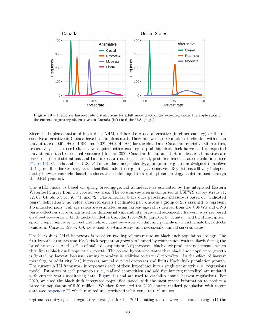
0
100
200
300
400
0.00 0.05 0.10Harvest rate
Fre
quen
cy
Alternative
Closed
Restrictive
Moderate
Liberal
Canada
0
100
200
300
400
0.00 0.05 0.10Harvest rate
Fre
quen
cy
Alternative
Closed
Restrictive
Moderate
United States
Figure 10 – Predictive harvest rate distributions for adult male black ducks expected under the application ofthe current regulatory alternatives in Canada (left) and the U.S. (right).
Since the implementation of black duck AHM, neither the closed alternative (in either country) or the re-strictive alternative in Canada have been implemented. Therefore, we assume a prior distribution with meanharvest rate of 0.01 (±0.001 SE) and 0.021 (±0.0014 SE) for the closed and Canadian restrictive alternatives,respectively. The closed alternative requires either country to prohibit black duck harvest. The expectedharvest rates (and associated variances) for the 2021 Canadian liberal and U.S. moderate alternatives arebased on prior distributions and banding data resulting in broad, posterior harvest rate distributions (seeFigure 10). Canada and the U.S. will determine, independently, appropriate regulations designed to achievetheir prescribed harvest targets as identified under the regulatory alternatives. Regulations will vary indepen-dently between countries based on the status of the population and optimal strategy as determined throughthe AHM protocol.
The AHM model is based on spring breeding-ground abundance as estimated by the integrated EasternWaterfowl Survey from the core survey area. The core survey area is comprised of USFWS survey strata 51,52, 63, 64, 66, 67, 68, 70, 71, and 72. The American black duck population measure is based on “indicatedpairs”, defined as 1 individual observed equals 1 indicated pair whereas a group of 2 is assumed to represent1.5 indicated pairs. Fall age ratios are estimated using harvest age ratios derived from the USFWS and CWSparts collection surveys, adjusted for differential vulnerability. Age- and sex-specific harvest rates are basedon direct recoveries of black ducks banded in Canada, 1990–2019, adjusted by country- and band inscription-specific reporting rates. Direct and indirect band recoveries of adult and juvenile male and female black ducksbanded in Canada, 1990–2019, were used to estimate age- and sex-specific annual survival rates.
The black duck AHM framework is based on two hypotheses regarding black duck population ecology. Thefirst hypothesis states that black duck population growth is limited by competition with mallards during thebreeding season. As the effect of mallard competition (c2 ) increases, black duck productivity decreases whichthen limits black duck population growth. The second hypothesis states that black duck population growthis limited by harvest because hunting mortality is additive to natural mortality. As the effect of harvestmortality, or additivity (a1 ) increases, annual survival decreases and limits black duck population growth.The current AHM framework incorporates each of these hypotheses into a single parametric (i.e., regression)model. Estimates of each parameter (i.e., mallard competition and additive hunting mortality) are updatedwith current year’s monitoring data (Figure 11) and are used to establish annual harvest regulations. For2020, we used the black duck integrated population model with the most recent information to predict abreeding population of 0.50 million. We then forecasted the 2020 eastern mallard population with recentdata (see Appendix E) which resulted in a predicted value equal to 0.39 million.
Optimal country-specific regulatory strategies for the 2021 hunting season were calculated using: (1) the
28

black duck harvest objective (98% of long-term cumulative harvest); (2) current, country-specific regulatoryalternatives (see Figure 10); (3) current parameter estimates for mallard competition and additive mortality(see Figure 11); (4) 2020 median predictions of 0.50 million breeding black ducks and 0.39 million breedingmallards in the core survey area; and (5) the country-specific 2020 regulations (liberal in Canada and moderatein the U.S). The optimal regulatory choices are the liberal alternative in Canada and moderate alternativein the U.S. (Table 7).
9.2 Northern Pintails
In 2010, the Flyway Councils and the USFWS established an adaptive management framework to informnorthern pintail harvest decisions. The current protocol is based on: (1) an explicit harvest managementobjective; (2) regulatory alternatives that do not permit partial seasons (i.e., shorter pintail season within thegeneral duck season) or 3-bird daily bag limits; (3) a formal optimization process using stochastic dynamicprogramming (Williams et al. 2002); (4) harvest allocation on a national rather than Flyway-by-Flyway basis,with no explicit attempt to achieve a particular allocation of harvest among Flyways; and (5) current systemmodels. Details describing the historical development of the technical and policy elements of the northernpintail adaptive management framework can be found in the northern pintail harvest strategy document(U.S. Fish and Wildlife Service 2010).
The harvest-management objective for the northern pintail population is to maximize long-term cumulativeharvest, which inherently requires perpetuation of a viable population. This objective is specified undera constraint that provides for an open hunting season when the observed breeding population is ≥1.75million birds (based on the lowest observed breeding population size since 1985 of 1.79 million birds in 2002).The single objective and constraint, in conjunction with the regulatory alternatives were determined afteran intensive consultation process with the waterfowl management community. The resulting managementobjective serves to integrate and balance multiple competing objectives for pintail harvest management,including minimizing closed seasons, eliminating partial seasons, maximizing seasons with liberal seasonlength and greater than 1-bird daily bag limit, and minimizing large changes in regulations.
The adaptive management protocol considers a range of regulatory alternatives for pintail harvest manage-ment that includes a closed season, 1-bird daily bag limit, or 2-bird daily bag limit. The maximum pintailseason length depends on the general duck season framework (characterized as liberal, moderate, or restrictiveand varying by Flyway) specified by mallard or multi-stock AHM. An optimal pintail regulation is calculatedunder the assumption of a liberal mallard or multi-stock season length in all Flyways. However, if the season
● ● ●
●
●
●
●
●
●●
●●
●● ●
●
●
●
●
●
●●
●● ● ●
●●
● ●
● ●●
●
●
●
●
●
0
2
4
6
0.00025
0.00050
0.00075
0.00100
0.00125
2005 2010 2015
Last year of time series
Add
itivi
ty (
a1)
Mal
lard
com
petit
ion
(c2
)
Figure 11 – Updated median estimates of black duck harvest additivity (a1 ; top panel) and mallard competition(c2 ; bottom panel) parameters over time. Error bars represent 95% credibility intervals.
29

Table 7 – Black duck optimal regulatory strategiesa for Canada and the United States for the 2021 huntingseason predicated on a liberal alternative selected by Canada and a moderate alternative selected by the UnitedStates the previous year (2020). This strategy is based on current regulatory alternatives, black duck model, andthe objective of achieving 98% of the maximum, long-term cumulative harvest and to share the allocated harvest(i.e., parity) equitably between countries. The shaded cell indicates the regulatory prescription for each countryin 2021.
Canada MALLb
ABDUb 0.05 0.10 0.15 0.20 0.25 0.30 0.35 0.40 0.45 0.50 0.55 0.60 0.65 0.70 0.75 0.80 0.85 0.90
0.05 C C C C C C C C C C C C C C C C C C
0.10 M M C C C C C C C C C C C C C C C C
0.15 L M M M M M M M M M M M M M M M M M
0.20 L L L L L L L M M M M M M M M M M M
0.25 L L L L L L L L L L L L L L L L L L
0.30 L L L L L L L L L L L L L L L L L L
0.35 L L L L L L L L L L L L L L L L L L
0.40 L L L L L L L L L L L L L L L L L L
0.45 L L L L L L L L L L L L L L L L L L
0.50 L L L L L L L L L L L L L L L L L L
0.55 L L L L L L L L L L L L L L L L L L
0.60 L L L L L L L L L L L L L L L L L L
0.65 L L L L L L L L L L L L L L L L L L
0.70 L L L L L L L L L L L L L L L L L L
0.75 L L L L L L L L L L L L L L L L L L
0.80 L L L L L L L L L L L L L L L L L L
United States MALLb
ABDUb 0.05 0.10 0.15 0.20 0.25 0.30 0.35 0.40 0.45 0.50 0.55 0.60 0.65 0.70 0.75 0.80 0.85 0.90
0.05 C C C C C C C C C C C C C C C C C C
0.10 R R C C C C C C C C C C C C C C C C
0.15 R R R R R R R R R R R R R R R R R R
0.20 M M M M R R R R R R R R R R R R R R
0.25 M M M M M M M M M M M M R R R R R M
0.30 M M M M M M M M M M M M M M M M M M
0.35 M M M M M M M M M M M M M M M M M M
0.40 M M M M M M M M M M M M M M M M M M
0.45 M M M M M M M M M M M M M M M M M M
0.50 M M M M M M M M M M M M M M M M M M
0.55 M M M M M M M M M M M M M M M M M M
0.60 M M M M M M M M M M M M M M M M M M
0.65 M M M M M M M M M M M M M M M M M M
0.70 M M M M M M M M M M M M M M M M M M
0.75 M M M M M M M M M M M M M M M M M M
0.80 M M M M M M M M M M M M M M M M M M
a C = closed season, R = restrictive, M = moderate, L = liberal.b Mallard and black duck breeding population sizes (in millions).
30

Table 8 – Substitution rules in the Central and Mississippi Flyways for joint implementation of northern pintailand mallard harvest strategies. The mid-continent mallard AHM strategy stipulates the maximum season lengthfor pintails in the Central and Mississippi Flyways. The substitutions are used when the mid-continent mallardseason length is less than liberal. For example, if the pintail strategy calls for a liberal season length with a 2-birddaily bag limit, but the mid-continent mallard strategy calls for a restrictive season length, the recommendedpintail regulation for the Central and Mississippi Flyways would be restrictive in length with a 3-bird daily baglimit.
Pintail Mid-continent mallard adaptive harvest management season length
Regulation Closed Restrictive Moderate Liberal
Closed Closed Closed Closed Closed
Liberal 1 Closed Restrictive 3 Moderate 3 Liberal 1
Liberal 2 Closed Restrictive 3 Moderate 3 Liberal 2
length of the general duck season determined by mallard or multi-stock AHM is less than liberal in anyof the Flyways, then an appropriate pintail daily bag limit would be substituted for that Flyway. Thus, ashorter season length dictated by mallard or multi-stock AHM would result in an equivalent season lengthfor pintails, but with increased bag limit if the expected harvest remained within allowable limits.
Regulatory substitution rules have been developed for the Central and Mississippi Flyways, where the generalduck season length is driven by the mid-continent mallard AHM protocol (Table 8). These substitutions weredetermined by finding a pintail daily bag limit whose expected harvest was less than or equal to that called forunder the national recommendation. Thus, if the national pintail harvest strategy called for a liberal 2-birdbag limit, but the mid-continent mallard season length was moderate, the recommended pintail regulationfor the Central and Mississippi Flyways would be moderate in length with a 3-bird bag limit. Becauseseason lengths more restrictive than liberal are expected infrequently in the Atlantic and Pacific Flywaysunder current eastern multi-stock and western mallard AHM strategies, substitution rules have not yet beendeveloped for these Flyways. If shorter season lengths were called for in the Pacific or Atlantic Flyway, thensimilar rules would be specified for these Flyways and used to identify the appropriate substitution. In allcases, a substitution produces a lower expected harvest than the harvest allowed under the pintail strategy.
The current AHM protocol for pintails considers two population models. Each model represents an alternativehypothesis about the effect of harvest on population dynamics: one in which harvest is additive to naturalmortality, and another in which harvest is compensatory to natural mortality. The compensatory modelassumes that the mechanism for compensation is density-dependent post-harvest (winter) survival. Themodels differ only in how they incorporate the winter survival rate. In the additive model, winter survivalrate is a constant, whereas winter survival is density-dependent in the compensatory model. A completedescription of the model set used to predict pintail population change can be found in Appendix L. Modelweights for the pintail model set have been updated annually since 2007 by comparing model predictions withobserved survey results. As of 2019, model weights favor the hypothesis that harvest mortality is additive(57%). For 2020, we used the pintail model set to calculate a weighted average of 2.446 million (SE = 0.489million) on the observed scale. We updated the latitude model with recent data (see Appendix F) to forecastthe 2020 pintail breeding distribution (latitude) which resulted in a predicted value equal to 55.16 (SE = 1.73)degrees.
An optimal regulatory strategy for the 2021 hunting season was calculated for northern pintails using: (1) anobjective to maximize long-term cumulative harvest; (2) current regulatory alternatives and the closed-seasonconstraint; and (3) current population models and model weights. The resulting regulatory strategy includesoptions conditional on the regulatory alternative selected the previous hunting season (Figure 12). Based ona liberal, 1-bird daily bag limit, regulatory alternative selected for the 2020 hunting season and a predicted2020 breeding population size of 2.446 million pintails observed at a mean latitude of 55.16 degrees, theoptimal regulatory choice for the 2021 hunting season for all four Flyways is the liberal regulatory alternativewith a 1-bird daily bag limit (Table 9).
31

Latitude
BP
OP
in M
illio
ns
0
1
2
3
4
5
6
7
8
9
10
11
12
13
14
15
52 54 56 58
Previous: Closed
52 54 56 58
Previous: Liberal 1
52 54 56 58
Previous: Liberal 2
Reg
C
L1
L2
Figure 12 – Northern pintail pre-survey harvest policies derived with updated optimization methods that accountfor changes in decision timing associated with adaptive harvest management protocols specified in the SEIS 2013.This strategy is based on current regulatory alternatives, current population models and their weights, and anobjective to maximize long-term cumulative harvest.
Table 9 – Northern pintail optimal regulatory strategya for the 2021 hunting season predicated on a liberalseason and a 1-bird daily bag limit selected the previous year (2020). This strategy is based on current regulatoryalternatives, northern pintail models and weights, and the objective of maximizing long-term cumulative harvestconstrained to provide for an open hunting season when the observed breeding population is ≥1.75 million birds.The shaded cell indicates the regulatory prescription for 2021.
Mean latitudec
BPOPb 53 53.2 53.4 53.6 53.8 54 54.2 54.4 54.6 54.8 55 55.2 55.4 55.6 55.8 56 56.2 56.4 56.6 56.8 57
≤ 1.7 C C C C C C C C C C C C C C C C C C C C C
1.8 L1 L1 L1 L1 L1 L1 L1 L1 L1 L1 L1 L1 L1 L1 L1 L1 L1 L1 L1 L1 L1
1.9 L1 L1 L1 L1 L1 L1 L1 L1 L1 L1 L1 L1 L1 L1 L1 L1 L1 L1 L1 L1 L1
2 L1 L1 L1 L1 L1 L1 L1 L1 L1 L1 L1 L1 L1 L1 L1 L1 L1 L1 L1 L1 L1
2.1 L1 L1 L1 L1 L1 L1 L1 L1 L1 L1 L1 L1 L1 L1 L1 L1 L1 L1 L1 L1 L1
2.2 L1 L1 L1 L1 L1 L1 L1 L1 L1 L1 L1 L1 L1 L1 L1 L1 L1 L1 L1 L1 L1
2.3 L1 L1 L1 L1 L1 L1 L1 L1 L1 L1 L1 L1 L1 L1 L1 L1 L1 L1 L1 L1 L1
2.4 L1 L1 L1 L1 L1 L1 L1 L1 L1 L1 L1 L1 L1 L1 L1 L1 L1 L1 L1 L1 L1
2.5 L2 L2 L2 L2 L2 L1 L1 L1 L1 L1 L1 L1 L1 L1 L1 L1 L1 L1 L1 L1 L1
2.6 L2 L2 L2 L2 L2 L2 L2 L2 L2 L2 L2 L2 L2 L2 L2 L2 L2 L2 L2 L2 L1
2.7 L2 L2 L2 L2 L2 L2 L2 L2 L2 L2 L2 L2 L2 L2 L2 L2 L2 L2 L2 L2 L2
2.8 L2 L2 L2 L2 L2 L2 L2 L2 L2 L2 L2 L2 L2 L2 L2 L2 L2 L2 L2 L2 L2
2.9 L2 L2 L2 L2 L2 L2 L2 L2 L2 L2 L2 L2 L2 L2 L2 L2 L2 L2 L2 L2 L2
≥3 L2 L2 L2 L2 L2 L2 L2 L2 L2 L2 L2 L2 L2 L2 L2 L2 L2 L2 L2 L2 L2
a C = closed season, L1 = liberal season with 1-bird daily bag limit, L2 = liberal season with 2-bird daily bag limit.b Observed northern pintail breeding population size (in millions) from the WBPHS (strata 1–18, 20–50, 75–77).c Mean latitude (in degrees) is the average latitude of the WBPHS strata weighted by population size.
32

Table 10 – Regulatory alternativesa and total expected harvest levels corresponding to the closed, restrictive,moderate, and liberal packages considered in the scaup adaptive harvest management decision framework.
Package Atlantic Mississippi Central Pacific Expected Harvestc
Closed 0.04
Restrictive 20(2)/40(1)b 45(2)/15(1)b 39(2)/35(1)b 86(2) 0.20
Moderate 60(2) 60(3) 74(3) 86(3) 0.35
Liberal 60(4) 60(4) 74(6) 107(7) 0.60
a Season length in days (daily bag limit); these alternatives assume an overall liberal adaptive harvest managementframework as determined by the status of mallards or multiple stocks in the Atlantic Flyway.
b Multiple day and daily bag limit combinations refer to hybrid seasons which allow for different daily bag limits over acontinuous season length.
c Total harvest in millions (Canada and United States combined).
9.3 Scaup
The USFWS implemented an AHM decision-making framework to inform scaup harvest regulations in 2008(Boomer and Johnson 2007). Prior to the implementation of the SEIS 2013, the scaup AHM protocol firstderived optimal harvest levels which were then used to determine the recommended regulatory package. Eachyear, an optimization was performed to identify the optimal harvest level based on updated scaup populationparameters. The harvest regulation was then determined by comparing the optimal harvest level to theharvest thresholds corresponding to restrictive, moderate, and liberal packages (see Boomer et al. 2007). Dueto the changes in decision timing associated with the SEIS, these procedures are not possible because decisionmakers would have to condition their regulatory decision on the harvest levels observed during the previoushunting season and this information would not be available. As a result, the decision variable (harvest) inthe scaup optimization was changed from harvest levels to a set of packages with associated expected harvestlevels in the updated optimization methods. We used the thresholds identified in Boomer et al. (2007) tospecify expected harvest levels for each package (Table 10). To account for partial controllability of the scaupharvest, we assumed that the harvest under each package could be represented with a normal distributionwith the mean set to the expected harvest level, assuming a coefficient of variation equal to 20%.
Initial scaup regulatory alternatives associated with restrictive, moderate, and liberal packages were developedbased on a simulation of an optimal policy derived under an objective to achieve 95% of the maximum,long-term cumulative harvest (Boomer et al. 2007). This objective resulted in a strategy less sensitive tosmall changes in population size compared to a strategy derived under an objective to achieve 100% ofthe maximum, long-term cumulative harvest and allowed for some harvest opportunity at relatively lowpopulation sizes. The USFWS worked with the Flyways to specify Flyway-specific regulatory alternativesto achieve the allowable harvest thresholds corresponding to each package. At this time, the USFWS alsoagreed to consider “hybrid season” options that would be available to all Flyways for the restrictive andmoderate packages. Hybrid seasons allow daily bag limits to vary for certain continuous portions of the scaupseason length. In 2008, restrictive, moderate, and liberal scaup regulatory alternatives were defined andimplemented in all four Flyways. Subsequent feedback from the Flyways led the USFWS to further clarifycriteria associated with the establishment of “hybrid seasons” and to allow additional modifications of thealternatives for each Flyway resulting in updated regulatory alternatives that were adopted in 2009. Becauseof the considerable uncertainty involved with predicting scaup harvest, the USFWS and the Flyways agreedto keep these packages in place for at least 3 years. In 2013, the moderate packages for the Mississippi andCentral Flyways were modified to include a 3-bird daily bag limit.
The lack of scaup demographic information over a sufficient time frame and at a continental scale precludesthe use of a traditional balance equation to represent scaup population and harvest dynamics. As a result, weused a discrete-time, stochastic, logistic-growth population model to represent changes in scaup abundance,while explicitly accounting for scaling issues associated with the monitoring data. Details describing themodeling and assessment framework that has been developed for scaup can be found in Appendix M and in
33

Boomer and Johnson (2007).
We updated the scaup assessment based on the current model formulation and data extending from 1974through 2019 and predicted the 2020 breeding population size equal to a median 3.53 million (SE = 0.37 ).As in past analyses, the state-space formulation and Bayesian analysis framework provided reasonable fitsto the observed breeding population and total harvest estimates with realistic measures of variation. Theposterior mean estimate of the intrinsic rate of increase (r) is 0.13 while the posterior mean estimate of thecarrying capacity (K ) is 8.76 million birds. The posterior mean estimate of the scaling parameter (q) is 0.76,ranging between 0.68 and 0.84 with 95% probability.
An optimal regulatory strategy for the 2021 hunting season was calculated for scaup using: (1) an objective toachieve 95% of the maximum, long-term cumulative harvest; (2) current regulatory alternatives; and (3) thecurrent population model and updated parameter estimates. The resulting regulatory strategy includes op-tions conditional on the regulatory alternative selected the previous hunting season (Table 11). We simulatedthe use of this regulatory strategy to determine expected performance characteristics. Assuming that har-vest management adhered to this strategy (and that current model parameters accurately reflect populationdynamics), breeding-population size would be expected to average 4.95 million (SD = 0.87 million). Basedon a restrictive regulatory alternative selected for the 2020 hunting season and a predicted 2020 breedingpopulation size of 3.53 million scaup, the optimal regulatory choice for the 2021 hunting season for all fourFlyways is the restrictive regulatory alternative (see Table 11).
10 EMERGING ISSUES IN ADAPTIVE HARVEST MANAGE-MENT
Learning occurs passively with current AHM protocols as annual comparisons of model predictions to ob-servations from monitoring programs are used to update model weights and relative beliefs about systemresponses to management (Johnson et al. 2002) or as model parameters are updated based on an assessmentof the most recent monitoring data (Boomer and Johnson 2007, Johnson et al. 2007). However, learning canalso occur as decision-making frameworks are evaluated to determine if objectives are being achieved, havechanged, or if other aspects of the decision problem are adequately being addressed. Often the feedback re-sulting from this process results in a form of “double-loop” learning (Lee 1993) that offers the opportunity toadapt decision-making frameworks in response to a shifting decision context, novel or emerging managementalternatives, or a need to revise assumptions and models that may perform poorly or need to account for newinformation. Adaptive management depends on this iterative process to ensure that decision-making proto-cols remain relevant in evolving biological and social systems. Throughout the waterfowl harvest managementcommunity, substantial progress has been made to outline the important issues that must be considered inthe revision of each AHM protocol (Johnson et al. 2015). In response to these large-scale issues, the HMWGhas been focusing efforts on the evolving needs of AHM and the role of the working group in planning forand executing the double-loop learning phase of AHM in relation to various decision-making frameworks.
In addition, the HMWG has been discussing the technical challenges involved with dealing with large-scalehabitat and environmental change on the decision-making frameworks used to inform waterfowl harvestmanagement. We anticipate that large-scale system change will exacerbate most forms of uncertainty thataffect waterfowl AHM, but we believe that the elements of the current AHM framework provide the necessarystructure for coping with these changing systems (Nichols et al. 2011).
The 2019 HMWGmeeting focused on the evaluation of the Central Flyway’s proposal for a two-tier regulationssystem along with revisions to northern pintail AHM (U.S. Fish and Wildlife Service 2019a). The HMWGproposed changes to the timing of how HMWG priorities are evaluated and established, by including a mid-summer conference call among working group members to discuss progress and current HMWG priorities.After this year’s July conference call, the HMWG proposed an updated set of fiscal year (FY2021) prioritiesfor 2021 (Appendix C).
34

Table 11 – Scaup optimal regulatory strategya for the 2021 hunting season. This strategy is based on thecurrent scaup population model and an objective to achieve 95% of the maximum, long-term cumulative harvest.Predicated on a restrictive regulatory alternative selected the previous year (2020), the shaded cell indicates theregulatory prescription for the 2021 hunting season.
Previous Regulation
BPOPb Closed Restrictive Moderate Liberal
≤2.7 C C C C
2.8 C C C C
2.9 R C C C
3.0 R R C C
3.1 R R R C
3.2 R R R C
3.3 R R R R
3.4 R R R R
3.5 R R R R
3.6 R R R R
3.7 R R R R
3.8 R R R R
3.9 R R R R
4.0 R R R R
4.1 M R R R
4.2 M R R R
4.3 M M R R
4.4 M M M R
4.5 M M M R
4.6 M M M M
4.7 M M M M
4.8 M M M M
4.9 M M M M
5.0 M M M M
5.1 M M M M
5.2 M M M M
5.3 M M M M
5.4 M M M M
5.5 L M M M
5.6 L M M M
5.7 L L M M
5.8 L L L M
5.9 L L L M
≥6 L L L L
a C = closed season, R = restrictive, M = moderate, L = liberal.b Estimated scaup breeding population (in millions) observed in the WBPHS (strata 1–18, 20–50, 75–77).
35

LITERATURE CITEDAnderson, D. R., and K. P. Burnham. 1976. Population ecology of the mallard. VI. The effect of exploitationon survival. U.S. Fish and Wildlife Service Resource Publication. 128. 66pp.
Balkcom, G. D., P. R. Garrettson, and P. I. Padding. 2010. Predicting wood duck harvest rates in EasternNorth America. Journal of Wildlife Management 74:1575–1579.
Blohm, R. J. 1989. Introduction to harvest – understanding surveys and season setting. Proceedings of theInternational Waterfowl Symposium 6:118–133.
Blohm, R. J., R. E. Reynolds, J. P. Bladen, J. D. Nichols, J. E. Hines, K. P. Pollock, and R. T. Eberhardt.1987. Mallard mortality rates on key breeding and wintering areas. Transactions of the North AmericanWildilfe and Resources Conference 52:246–263.
Boomer, G. S., and F. A. Johnson. 2007. A proposed assessment and decision-making frameworkto inform scaup harvest management. Unpublished Report. U.S. Fish and Wildlife Service, Laurel,MD. 26pp. URL http://www.fws.gov/migratorybirds/NewReportsPublications/SpecialTopics/BySpecies/
SCAUP2007Report.pdf.
Boomer, G. S., F. A. Johnson, M. D. Koneff, T. A. Sanders, and R. E. Trost. 2007. A process to determinescaup regulatory alternatives. Unpublished Scoping Document. U.S. Fish and Wildlife Service, Laurel,MD. 20pp. URL http://www.fws.gov/migratorybirds/NewReportsPublications/SpecialTopics/BySpecies/
scaup_regs_scoping_draftVI.pdf.
Boomer, G. S., F. A. Johnson, and G. S. Zimmerman. 2015. Adaptive harvest management: adjust-ments for SEIS 2013. U. S. Department of Interior, Washington, D. C. 21pp. URL http://www.fws.gov/
migratorybirds/pdf/management/AHM/SEIS&AHMReportFinal.pdf.
Boomer, G. S., G. S. Zimmerman, P. R. Garrettson, M. D. Koneff, T. A. Sanders, K. D. Magruder, andJ. A. Royle. 2013. Band reporting probabilities for mallards recovered in the United States and Canada.Journal of Wildlife Management 77:1059–1066.
Brooks, S. P., and A. Gelman. 1998. Alternative methods for monitoring convergence of iterative simulations.Journal of Computational and Graphical Statistics 7:434–455.
Burnham, K. P., G. C. White, and D. R. Anderson. 1984. Estimating the effect of hunting on annual survivalrates of adult mallards. Journal of Wildlife Management 48:350–361.
Conroy, M. J. 2010. Technical support for adaptive harvest management for American black ducks. Unpub-lished Final Report. Cooperative Fish and Wildlife Research Unit, U.S. Geological Survey, Warnell Schoolof Forestry and Natural Resources, University of Georgia, Athens, GA.
Fackler, P. 2011. User’s Guide, MDPSOLVE: A MATLAB Toolbox for Solving Markov Decision Problemswith Dynamic Programming.
Garrettson, P. R., R. V. Raftovich, J. E. Hines, and G. S. Zimmerman. 2013. Band reporting probabili-ties of mallards, American black ducks, and wood ducks in eastern North America. Journal of WildlifeManagement 78:50–57.
Henny, C. J., and K. P. Burnham. 1976. A reward band study of mallards to estimate reporting rates.Journal of Wildlife Management 40:1–14.
Heusmann, H. W., and J. R. Sauer. 2000. The northeastern states’ waterfowl breeding population survey.Wildlife Society Bulletin 28:355–364.
Hodges, J. L., J. G. King, B. Conant, and H. A. Hanson. 1996. Aerial surveys of waterbirds in Alaska1975–94: population trends and observer variability. National Biological Service, U.S. Department of theInterior Information and Technology Report 4, Washington, D.C.
36

Hyndman, R. J., and G. Athanasopoulos. 2018. Forecasting: principles and practice, 2nd edition. OTexts:Melbourne, Australia, OTexts.com/fpp2. Accessed on 14 July 2020.
Johnson, F. A. 2003. Population dynamics of ducks other than mallards in mid-continent North America.Draft. U.S. Fish and Wildlife Service, U.S. Department of the Interior, Washington, D.C. 15pp.
Johnson, F. A., G. S. Boomer, and T. A. Sanders. 2007. A proposed protocol for the adaptive harvestmanagement of mallards breeding in Western North America. Unpublished Report. U.S. Fish and WildlifeService, Laurel, MD. 33pp.
Johnson, F. A., G. S. Boomer, B. K. Williams, J. D. Nichols, and D. J. Case. 2015. Multilevel Learningin the Adaptive Management of Waterfowl Harvests: 20 Years and Counting. Wildlife Society Bulletin39:9–19. URL http://dx.doi.org/10.1002/wsb.518.
Johnson, F. A., P. L. Fackler, G. S. Boomer, G. S. Zimmerman, B. K. Williams, J. D. Nichols, and R. M.Dorazio. 2016. State-dependent resource harvesting with lagged information about system states. PLoSONE 11:1–21. URL http://dx.doi.org/10.1371%2Fjournal.pone.0157373.
Johnson, F. A., W. L. Kendall, and J. A. Dubovsky. 2002. Conditions and limitations on learning in theadaptive management of mallard harvests. Wildlife Society Bulletin 30:176–185.
Johnson, F. A., C. T. Moore, W. L. Kendall, J. A. Dubovsky, D. F. Caithamer, J. Kelley, J. R., and B. K.Williams. 1997. Uncertainty and the management of mallard harvests. Journal of Wildlife Management61:202–216.
Johnson, F. A., M. A. Walters, and G. S. Boomer. 2012. Allowable levels of take for the trade in Nearcticsongbirds. Ecological Applications 22:1114–1130. URL https://esajournals.onlinelibrary.wiley.com/
doi/abs/10.1890/11-1164.1.
Johnson, F. A., B. K. Williams, J. D. Nichols, J. E. Hines, W. L. Kendall, G. W. Smith, and D. F. Caithamer.1993. Developing an adaptive management strategy for harvesting waterfowl in North America. Transac-tions of the North American Wildlife and Natural Resources Conference 58:565–583.
Johnson, F. A., B. K. Williams, and P. R. Schmidt. 1996. Adaptive decision-making in waterfowl harvestand habitat management. Proceedings of the International Waterfowl Symposium 7:26–33.
Lee, K. N. 1993. Compass and Gyroscope: Integrating Science and Politics for the Environment. IslandPress, Washington, D.C.
Martin, E. M., and S. M. Carney. 1977. Population ecology of the mallard. IV. A review of duck huntingregulations, activity, and success, with special reference to the mallard. U.S. Fish and Wildlife Service,Washington D.C.
MATLAB. 2016. Version 9.0.0.341360 (R2016a). The MathWorks Inc., Natick, Massachusetts.
Meyer, R., and R. B. Millar. 1999. BUGS in Bayesian stock assessments. Canadian Journal of Fisheries andAquatic Sciences 56:10078–1086.
Millar, R. B., and R. Meyer. 2000. Non-linear state space modeling of fisheries biomass dynamics by usingMetropolis-Hastings within Gibbs sampling. Applied Statistics 49:327–342.
Nichols, J. D., F. A. Johnson, and B. K. Williams. 1995a. Managing North American waterfowl in the faceof uncertainty. Annual Review of Ecology and Systematics 26:177–199.
Nichols, J. D., M. D. Koneff, P. J. Heglund, M. G. Knutson, M. E. Seamans, J. E. Lyons, J. M. Morton,M. T. Jones, G. S. Boomer, and B. K. Williams. 2011. Climate change, uncertainty, and natural resourcemanagement. Journal of Wildlife Management 75:6–18.
Nichols, J. D., R. E. Reynolds, R. J. Blohm, R. E. Trost, J. E. Hines, and J. P. Bladen. 1995b. Geographicvariation in band reporting rates for mallards based on reward banding. Journal of Wildlife Management59:697–708.
37

Niel, C., and J.-D. Lebreton. 2005. Using demographic invariants to detect overharvested bird populationsfrom incomplete data. Conservation Biology 19:826–835. URL http://www.jstor.org/stable/3591072.
Padding, P. I., G. S. Zimmerman, M. T. Huang, G. D. Balkcom, and P. K. Devers. 2018. A multi-stockadaptive harvest management protocol for informing annual harvest regulations in the Atlantic Flyway.Unpublished Final Report. U.S. Fish and Wildlife Service Division of Migratory Bird Management and theAtlantic Flyway.
Plummer, M., 2003. JAGS: A program for analysis of Bayesian graphical models using Gibbs sampling. Pages1–10 in K. Hornik, F. Leisch, and A. Zeileis, editors. Proceedings of the 3rd international workshop ondistributed statistical computing (DSC 2003). Vienna, Austria.
Runge, M. C. 2007. Northern pintail harvest strategy: development of a compensatory model. UnpublishedReport. U.S. Geological Survey, Patuxent Wildlife Research Center, Laurel, MD.
Runge, M. C., and G. S. Boomer. 2005. Population dynamics and harvest management of the continentalnorthern pintail population. Unpublished Report. U.S. Geological Survey, Patuxent Wildlife ResearchCenter, Laurel, MD. 42pp.
Runge, M. C., F. A. Johnson, J. A. Dubovsky, W. L. Kendall, J. Lawrence, and J. Gammonley. 2002. Arevised protocol for the adaptive harvest management of mid-continent mallards. U.S. Fish and WildlifeService, U.S. Department of the Interior Technical report, Washington, D.C. URL http://www.fws.gov/
migratorybirds/NewReportsPublications/AHM/Year2002/MCMrevise2002.pdf.
Runge, M. C., W. L. Kendall, and J. D. Nichols, 2004. Exploitation. in W. J. Sutherland and R. Green,editors. Bird Ecology and Conservation: A Handbook of Techniques. Oxford University Press, Inc., Oxford,UK.
Schaefer, M. B. 1954. Some aspects of the dynamics of populations important to the management ofcommercial marine fisheries. Bulletin of the Inter-American Tropical Tuna Commission 1:25–56.
Smith, G. W. 1995. A critical review of the aerial and ground surveys of breeding waterfowl in North America.National Biological Service, U.S. Department of the Interior Biological Science Report 5, Washington, D.C.
Spiegelhalter, D. J., A. Thomas, N. Best, and D. Lunn. 2003. WinBUGS 1.4 User manual. MRC BiostatisticsUnit, Institues of Public Health, Cambridge, UK.
U.S. Department of the Interior. 2013. Final Supplemental Environmental Impact Statement: Issuance ofAnnual Regulations Permitting the Hunting of Migratory Birds. U.S. Fish and Wildlife Service, Wash-ington, D.C. 418pp. URL http://www.fws.gov/migratorybirds/pdfs/FSEIS%20Issuance%20of%20Annual%
20Regulations%20Permitting%20the%20Hunting%20of%20Migratory%20Birds.pdf.
U.S. Fish and Wildlife Service. 2000. Adaptive harvest management: 2000 duck hunting sea-son. U.S. Department of Interior, Washington, D.C. 43pp. URL http://www.fws.gov/migratorybirds/
NewReportsPublications/AHM/Year2000/ahm2000.pdf.
U.S. Fish and Wildlife Service. 2001. Framework-date extensions for duck hunting in the United States:projected impacts & coping with uncertainty. U.S. Department of Interior, Washington, D.C. 8pp. URLhttp://www.fws.gov/migratorybirds/NewReportsPublications/AHM/Year2001/fwassess.PDF.
U.S. Fish and Wildlife Service. 2002. Adaptive harvest management: 2002 duck hunting sea-son. U.S. Department of Interior, Washington, D.C. 34pp. URL http://www.fws.gov/migratorybirds/
NewReportsPublications/AHM/Year2002/2002-AHM-report.pdf.
U.S. Fish and Wildlife Service. 2010. Northern Pintail Harvest Strategy. U.S. Department of Interior, Wash-ington, D.C. 20pp. URL http://www.fws.gov/migratorybirds/NewReportsPublications/SpecialTopics/
BySpecies/Nopi%20Harvest%20Strategy%202010%20Final.pdf.
38
U.S. Fish and Wildlife Service. 2017. Adaptive harvest management: 2018 hunting season. U.S. Depart-ment of Interior, Washington, D.C. 58pp. URL https://www.fws.gov/migratorybirds/pdf/management/AHM/
AHMReport2018.pdf.
U.S. Fish and Wildlife Service. 2019a. Harvest Management Working Group: 2019 Annual Meeting Report.U.S. Department of Interior, Washington, D.C. 41pp. URL https://www.fws.gov/migratorybirds/pdf/
management/AHM/HMWGReport2019.pdf.
U.S. Fish and Wildlife Service. 2019b. Waterfowl population status, 2019. U.S. Department of Interior,Washington, D.C. URL https://www.fws.gov/migratorybirds/pdf/surveys-and-data/Population-status/
Waterfowl/WaterfowlPopulationStatusReport19.pdf.
Walters, C. 1986. Adaptive Management of Renewable Resources. Macmillian, New York.
Williams, B. K., and F. A. Johnson. 1995. Adaptive management and the regulation of waterfowl harvests.Wildlife Society Bulletin 23:430–436.
Williams, B. K., F. A. Johnson, and K. Wilkins. 1996. Uncertainty and the adaptive management of waterfowlharvests. Journal of Wildlife Management 60:223–232.
Williams, B. K., J. D. Nichols, and M. J. Conroy. 2002. Analysis and Management of Animal Populations.Academic Press, San Diego, CA.
Zimmerman, G. S., J. R. Sauer, K. Fleming, W. A. Link, and P. R. Garrettson. 2015. Combining waterfowland breeding bird survey data to estimate wood duck breeding population size in the Atlantic Flyway.Journal of Wildlife Management 79:1051–1061.
Zimmerman, G. S., J. R. Sauer, W. A. Link, and M. Otto. 2012. Composite analysis of black duck breedingpopulation surveys in eastern North America. Journal of Wildlife Management 76:1165–1176.
39
Appendix A Harvest Management Working Group Members
This list includes only permanent members of the Harvest Management Working Group. Not listed here arenumerous persons from federal and state agencies that assist the Working Group on an ad-hoc basis.
Coordinator:
Scott Boomer
U.S. Fish & Wildlife Service
11510 American Holly Drive
Laurel, Maryland 20708-4017
phone: 301-497-5684; fax: 301-497-5871
e-mail: scott [email protected]
USFWS Representatives:
Nanette Seto (Region 1) Scott Carleton (Region 2)
U.S. Fish & Wildlife Service U.S. Fish & Wildlife Service
911 NE 11TH Avenue 500 Gold SW - 8th Floor
Portland, OR 97232-4181 Albuquerque, NM 87103
phone: 503 231-6159 phone: 505-248-6639
fax: 503 231-2019 fax: 505-248-7885
e-mail: nanette [email protected] e-mail: scott [email protected]
Tom Cooper (Region 3) Bill Uihlein (Region 4)
U.S. Fish & Wildlife Service U.S. Fish & Wildlife Service
5600 American Blvd West 1875 Century Blvd.
Bloomington, MN 55437-1458 Atlanta, GA 30345
phone: 612-713-5101 phone: 404-679-7288
fax: 612-713-5393 fax: 404 679-4180
e-mail: tom [email protected] e-mail:bill [email protected]
Pam Toschik (Region 5) Brian Smith (Region 6)
U.S. Fish & Wildlife Service U.S. Fish & Wildlife Service
300 Westgate Center Drive P.O. Box 25486-DFC
Hadley, MA 01035-9589 Denver, CO 80225-0486
phone: 413-253-8610 phone: 303-236-4403
fax: 413-253-8293 fax: 303-236-8680
e-mail:pamela [email protected] e-mail:brian w [email protected]
Eric Taylor (Region 7) Amedee Brickey (Region 8)
U.S. Fish & Wildlife Service U.S. Fish & Wildlife Service
1011 East Tudor Road 2800 Cottage Way, W-2606
Anchorage, AK 99503-6119 Sacramento, CA 95825
phone: 907-786-3446 phone: 916-414-6480
40

fax: 907-786-3641 fax: 916-414-6486
e-mail: eric [email protected] e-mail: amedee [email protected]
Kathy Fleming (Headquarters) Pat Devers (Headquarters)
Chief, Branch of Monitoring and Data Management Chief, Branch of Assessment and Decision Support
U.S. Fish & Wildlife Service U.S. Fish & Wildlife Service
11510 American Holly Drive 11510 American Holly Drive
Laurel, Maryland 20708-4017 Laurel, Maryland 20708-4017
phone: phone:
fax: 301-497-5871 fax: 301-497-5871
e-mail: kathy [email protected] e-mail: pat [email protected]
Atlantic Flyway Representative (Headquarters) Mississippi Flyway Representative (Headquarters)
U.S. Fish & Wildlife Service U.S. Fish & Wildlife Service
Vacant Vacant
Jim Dubovsky (Headquarters) Todd Sanders (Headquarters)
Central Flyway Representative Pacific Flyway Representative
U.S. Fish & Wildlife Service U.S. Fish & Wildlife Service
134 Union Blvd., Suite 540 1211 SE Cardinal Court, Suite 100
Lakewood, CO 80228 Vancouver, WA 98683
phone: 303-275-2386 phone: 360-604-2562
fax: 303-275-2384 fax: 360-604-2505
e-mail: james [email protected] e-mail: todd [email protected]
Canadian Wildlife Service Representatives:
Christian Roy Vacant
Canadian Wildlife Service Canadian Wildlife Service
351 Saint-Joseph Blvd, Suite 150, 123 Main Street
Gatineau, Que, K1A 0H3 Winnipeg, MB R3C 4W2
phone: 819-938-5418 phone:
fax: fax:
e-mail:[email protected] e-mail:
Flyway Council Representatives:
Min Huang (Atlantic Flyway) Greg Balkcom (Atlantic Flyway)
CT Dept. of Environmental Protection GA Dept. of Natural Resources
Franklin Wildlife Mgmt. Area 1014 Martin Luther King Blvd.
391 Route 32 North Franklin, CT 06254 Fort Valley, GA 31030
phone: 860-642-6528 phone: 478-825-6354
fax: 860-642-7964 fax: 478-825-6421
e-mail: [email protected] e-mail:[email protected]
41

John Brunjes (Mississippi Flyway) Adam Phelps (Mississippi Flyway)
Kentucky Dept. Of Fish and Wildlife Resources Indiana Division of Fish and Wildlife
# 1 Sportsman’s Lane 5596 E State Road 46
Frankfort, KY 40601 Bloomington, IN 47401
phone: 502-892-4500 phone: 812-334-1137
fax: fax: 812-339-4807
e-mail: [email protected] e-mail: [email protected]
Mike Szymanski (Central Flyway) Kevin Kraai (Central Flyway)
North Dakota Game and Fish Department Texas Parks and Wildlife Department
100 North Bismarck Expressway P.O. Box 659
Bismarck, ND 58501-5095 Canyon, TX 79015
phone: 701-328-6360 phone: 806-651-3011
fax: 701-328-6352 fax:
e-mail: [email protected] email: [email protected]
Brandon Reishus (Pacific Flyway) Jason Schamber (Pacific Flyway)
Oregon Dept of Fish and Wildlife Alaska Dept. Fish & Game
4034 Fairview Industrial Dr. SE 525 W. 67th Ave
Salem, OR 97302 Anchorage, AK 99518
phone: 503-947-6324 phone: 907-267-2206
fax: 503-947-6330 fax: 907-267-2859
e-mail: [email protected] e-mail: [email protected]
USGS Scientist:
Mike Runge (USGS)
Patuxent Wildlife Research Center
U.S. Geological Survey
12100 Beech Forest Rd. Laurel, MD 20708
phone: 301-497-5748
fax: 301-497-5545
e-mail: [email protected]
42

Appendix B 2021-2022 Regulatory Schedule
SCHEDULE OF BIOLOGICAL INFORMATION AVAILABILITY, REGULATIONS MEETINGS AND FEDERAL REGISTER PUBLICATIONS FOR THE 2021–22 HUNTING SEASON
April 28, 2020 - Video-teleconference PROPOSED RULEMAKING (PRELIMINARY)SRC Meeting WITH STATUS INFORMATION
and ISSUES
August 15 - September 30, 2020Flyway Tech And Council Meetings
HUNTER ACTIVITY and HARVEST REPORT
February 25, 2021FINAL SEASON FRAMEWORKS
March 2021 (at North American Conference)
June 1, 2021ALL HUNTING SEASONS SELECTIONS
(Season Selections Due April 30)
Flyway Council Meetings
July 10, 2020
INFORMATION for CRANES
SRC Regulatory Meeting
and WATERFOWL
SPRING POPULATION SURVEYSMarch–June, 2020
August 15, 2020WATERFOWL STATUS REPORT
WEBLESS and CRANE STATUSINFORMATION, DOVE and WOODCOCK
SUPPLEMENTAL PROPOSALS
August 20, 2020AHM REPORT w/OPTIMAL ALTERNATIVES,
PROPOSED SEASON FRAMEWORKS
September 1, 2021 and laterALL HUNTING SEASONS
October 20-21, 2020 - Virtual
December 15, 2020–January 31, 2021
REGULATORY ALTERNATIVES, and
September 15, 2020
MEETING SCHEDULE FEDERAL REGISTER SCHEDULE
December 10, 2020
(30 Day Comment Period)
FALL and WINTER SURVEY
SURVEY & ASSESSMENT SCHEDULE
Figure B.1 – Schedule of biological information availability, regulation meetings, and Federal Register publica-tions for the 2021–2022 hunting season.
43

Appendix C
Proposed FY2021 Harvest Management Working Group Priorities
Table C.1 – Priority rankings and project leads identified for the technical work proposed at the 2019 HarvestManagement Working Group meeting and updated during the summer of 2020.
Priority Level Status Participants
Highest Priorities (Urgent and Important)
Evaluation of Experimental two-tier license system On-going Central Flyway, DMBM
Northern Pintail AHM revision On-going DMBM, Flyway Councils,USGS
Reconsideration of North American Duck Harvest Management On-going DMBM, Flyway Councils
Development of an Eastern mallard harvest strategy On-going Atlantic Flyway Council,DMBM
Re-invigorating institutional support for AHM On-going DMBM, HMWG commu-nications team
Long-range Priorities (Non-urgent, but Very Important)
Time-dependent optimal solutions to address system change (e.g.,habitat change; hunter dynamics; climate change).
On-going USGS, BADS
Western mallard AHM revision On-going Pacific Flyway, BADS
Additional Priorities
Waterfowl Banding Needs Assessment On-going BADS, USGS, FlywayCouncils
Waterfowl harvest potential assessment methods case study de-velopment
On-going Atlantic Flyway Office,DMBM
44
Forecasting Canadian Ponds:Spring 2020
G. Scott Boomer
Branch of Assessment and Decision SupportDivision of Migratory Bird Management
U.S. Fish and Wildlife [email protected]
20 August 2020
Abstract
Due to the COVID-19 pandemic, waterfowl habitat conditions (ponds) were not directly observedin the spring of 2020. As a result, waterfowl harvest regulations will have to be informedwith information based on predictions of breeding population sizes and habitat conditions. Wedeveloped an estimation and forecasting framework to predict the number of Canadian ponds inthe spring of 2020 based on information that is available to decision makers during the 2020–2021regulations process. We summarized annual, total precipitation for prairie Canada and usedthis variable as a predictor in an autoregressive integrated moving average (ARIMA) estimationframework to develop a model to forecast the number of Canadian ponds in 2020. The top rankedmodel that was best supported by the data included a 1st order moving average term [ARIMA(0,0,1)]. Based on our selected model, the 2020 forecast of the number of Canadian ponds is 3.40million (95% PI = 1.75 – 5.06).
ContentsBackground . . . . . . . . . . . . . . . . . . . . . . . . . . . . . . . . . . . . . . . . . . . . .
Data . . . . . . . . . . . . . . . . . . . . . . . . . . . . . . . . . . . . . . . . . . . . . . . . . .
Time Series Analysis . . . . . . . . . . . . . . . . . . . . . . . . . . . . . . . . . . . . . . .
2020 Forecast . . . . . . . . . . . . . . . . . . . . . . . . . . . . . . . . . . . . . . . . . . . .
References . . . . . . . . . . . . . . . . . . . . . . . . . . . . . . . . . . . . . . . . . . . . . .
45

List of Tables1 Weather stations used to summarize total annual precipitation observed in prairie
Canada from 1961–2020 . . . . . . . . . . . . . . . . . . . . . . . . . . . . . . . . . .
List of Figures1 The number of ponds (millions) and total annual precipitation (mm) observed in
prairie Canada from 1961–2020. . . . . . . . . . . . . . . . . . . . . . . . . . . . . .2 Autocorrelation plots of Canadian ponds (millions) observed in prairie Canada from
1961–2019. . . . . . . . . . . . . . . . . . . . . . . . . . . . . . . . . . . . . . . . . .3 Regression and ARIMA residuals from the selected model [ARIMA(0,0,1)]. . . . . .4 Residual diagnostics from the selected model [ARIMA(0,0,1)]. . . . . . . . . . . . . .5 The 2020 forecast of Canadian ponds from an ARIMA(0,0,1) regression model. . . .
46

BackgroundDue to the COVID-19 pandemic, the United States Fish and Wildlife Service (USFWS) and its partnerswere unable to participate in the Waterfowl Breeding Population and Habitat Survey (WBPHS) toestimate the 2020 waterfowl breeding populations as well as evaluate breeding habitat conditions. Asa result, the promulgation of waterfowl harvest regulations in 2020 will require some modi�cationsto the adaptive harvest management (AHM) decision protocols that typically govern the regulatoryprocess. For example, observed breeding population estimates are used to determine optimal levelsof harvest. In the absence of this information, the USFWS proposes to base 2020 regulatory decisionson predictions of breeding population sizes and habitat conditions. Current system models forwhich we have AHM decision frameworks will be used to predict 2020 population sizes based on thebreeding population sizes, habitat conditions, harvest, and harvest rates observed in 2019. Underthe mid-continent mallard AHM decision framework, we use a 1st order autoregressive time seriesmodel to predict the number of Canadian ponds as a function of the number of ponds observed theprevious year. However, this model is based on data from 1961 – 2001 and there is interest in updatingthe original pond model that was developed for mid-continent mallard AHM with the availableinformation, including an additional predictor (total precipitation) that is available at the time decisionmakers will be considering regulatory decisions. As a result, we developed an estimation frameworkthat will predict the number of Canadian ponds as a function of the number of ponds observed in2019 and the total annual precipitation observed since the last WBPHS.
DataWe are interested in predicting the number of Canadian ponds for the 2020 breeding season from theavailable information for ponds observed in 2019 and the total amount of recorded precipitation fromprairie weather stations from 1 June 2019 through 31 May 2020. Based on earlier work (Pospahala et al.1974, Johnson et al. 1997), we selected weather stations from the Canadian prairies with continualobservations of daily precipitation totals from 1961–2020 (Table 1). We then summarized the numberof Canadian ponds observed in the traditional survey area of the Waterfowl Breeding Populationand Habitat Survey (U.S. Fish and Wildlife Service 2019). We then summed the total precipitationrecorded at the prairie weather stations from the 365 day period extending from 1 June to 31 May onthe year of the WBPHS (i.e., the 2019 total precipitation value would be the sum of daily precipitationvalues observed from 1 June 2018 through 31 May 2019).
From 1961–2020, total precipitation in the Canadian prairies varied from a low of 271 mm in 2018and a high of 563 mm in 1974 (Figure 1). The observed precipitation in 2020 was 394 mm.
47

Table 1: Weather stations used to summarize total annual precipitation observed in prairie Canadafrom 1961–2020
Province Station_Name Station_ID Start_year End_yearAlberta EDMONTON INT’L A 1865 1959 2012Alberta EDMONTON INT’L A 50149 2012 2020Alberta MEDICINE HAT A 2273 1883 2008Alberta MEDICINE HAT RCS 30347 2000 2020Manitoba BRANDON A 3471 1941 2012Manitoba BRANDON RCS 49909 2012 2020Manitoba WINNIPEG RICHARDSON INT’L A 3698 1938 2008Manitoba WINNIPEG A CS 27174 1996 2020Saskatchewan REGINA INT’L A 3002 1959 2013Saskatchewan REGINA RCS 28011 2012 2020Saskatchewan SASKATOON DIEFENBAKER INT’L A 3328 1883 2012Saskatchewan SASKATOON RCS 47707 2000 2020
pondsprecipitation
1960 1980 2000 2020
2
3
4
5
6
300
400
500
Year
Figure 1: The number of ponds (millions) and total annual precipitation (mm) observed in prairieCanada from 1961–2020.
We �rst examined autocorrelation plots to evaluate the information in the Canadian pond timeseries (Figure 2) and used an augmented Dickey-Fuller test from the tseries R package (Trapletti andHornik 2019) to analyze the time series for stationarity. The results from this test suggest there isevidence to reject the null hypothesis so we conclude that the data are stationary.
48

ggtsdisplay(window(cp_ts,end=2019)[,"ponds"],ylab="Canadian ponds")
2
3
4
5
6
1960 1970 1980 1990 2000 2010 2020
Can
adia
n po
nds
−0.2
−0.1
0.0
0.1
0.2
0.3
5 10 15Lag
AC
F
−0.2
−0.1
0.0
0.1
0.2
0.3
5 10 15Lag
PAC
F
Figure 2: Autocorrelation plots of Canadian ponds (millions) observed in prairie Canada from1961–2019.
#ggPacf(bwt_ts)
adf.test(window(cp_ts,end=2019)[,"ponds"],alternative="stationary",k=0)
## Warning in adf.test(window(cp_ts, end = 2019)[, "ponds"], alternative =
## "stationary", : p-value smaller than printed p-value
##
## Augmented Dickey-Fuller Test
##
## data: window(cp_ts, end = 2019)[, "ponds"]
## Dickey-Fuller = -5.3609, Lag order = 0, p-value = 0.01
## alternative hypothesis: stationary
To con�rm this result, we used a KPSS test that can account for a trend.
kpss.test(window(cp_ts,end=2019)[,"ponds"],null="Trend")
## Warning in kpss.test(window(cp_ts, end = 2019)[, "ponds"], null = "Trend"): p-
## value greater than printed p-value49

##
## KPSS Test for Trend Stationarity
##
## data: window(cp_ts, end = 2019)[, "ponds"]
## KPSS Trend = 0.10376, Truncation lag parameter = 3, p-value = 0.1
For the KPSS test, the null hypothesis is that the time series is stationary. Our test results provideslittle evidence to reject the null hypothesis that the pond time series is stationary, suggesting that wewill not have to consider di�erencing in our analysis.
Time Series AnalysisWe are interested in predicting the number of Canadian ponds for the 2020 breeding season as afunction of the number of ponds observed in 2019 and the total amount of recorded precipitation fromprairie weather stations from 1 June 2019 through 31 May 2020. We revisited the original formulationof the Canadian pond model developed for the mid-continent mallard AHM program (Johnson et al.1997). The predictive equation used to project the number of Canadian ponds (P) included
%C = V0 + U%C−1 + V1%A428?C + nCwhere, V0 is the intercept, U is the autoregressive term, V1 is the slope term for the precipitationcovariate and error term n is the assumed to be white noise.
We analyzed the updated information with an autoregressive integrated moving average (ARIMA)estimation framework, using the R function auto.arima from the forecast R package (Hyndman et al.2020, Hyndman and Khandakar 2008) to determine the appropriate number of lags and levels ofdi�erencing (Hyndman and Athanasopoulos 2018) for the �nal speci�cation of our ARIMA regressionmodel.
fit<-auto.arima(window(cp_ts,end=2019)[,"ponds"],xreg=window(cp_ts,end=2019)[,"precipitation"],stepwise=FALSE,
approximation=FALSE,
seasonal=FALSE,
trace=TRUE)
##
## ARIMA(0,0,0) with zero mean : 161.5068
## ARIMA(0,0,0) with non-zero mean : 163.3993
## ARIMA(0,0,1) with zero mean : 152.119
## ARIMA(0,0,1) with non-zero mean : 153.6019
## ARIMA(0,0,2) with zero mean : 153.751
## ARIMA(0,0,2) with non-zero mean : 155.6254
## ARIMA(0,0,3) with zero mean : 155.8635
## ARIMA(0,0,3) with non-zero mean : 157.9997
## ARIMA(0,0,4) with zero mean : 157.1322
## ARIMA(0,0,4) with non-zero mean : 159.6507
## ARIMA(0,0,5) with zero mean : 159.1683
## ARIMA(0,0,5) with non-zero mean : 161.6738
## ARIMA(1,0,0) with zero mean : 152.4232
## ARIMA(1,0,0) with non-zero mean : 154.4094
50

## ARIMA(1,0,1) with zero mean : 153.8641
## ARIMA(1,0,1) with non-zero mean : 155.6688
## ARIMA(1,0,2) with zero mean : 155.8828
## ARIMA(1,0,2) with non-zero mean : 157.6111
## ARIMA(1,0,3) with zero mean : 158.0459
## ARIMA(1,0,3) with non-zero mean : 160.3997
## ARIMA(1,0,4) with zero mean : 159.407
## ARIMA(1,0,4) with non-zero mean : 161.965
## ARIMA(2,0,0) with zero mean : 154.0319
## ARIMA(2,0,0) with non-zero mean : 155.9521
## ARIMA(2,0,1) with zero mean : 156.247
## ARIMA(2,0,1) with non-zero mean : 158.1479
## ARIMA(2,0,2) with zero mean : 158.3529
## ARIMA(2,0,2) with non-zero mean : 160.1859
## ARIMA(2,0,3) with zero mean : 160.304
## ARIMA(2,0,3) with non-zero mean : Inf
## ARIMA(3,0,0) with zero mean : 155.6994
## ARIMA(3,0,0) with non-zero mean : 157.4428
## ARIMA(3,0,1) with zero mean : 157.6636
## ARIMA(3,0,1) with non-zero mean : 159.3361
## ARIMA(3,0,2) with zero mean : 158.8419
## ARIMA(3,0,2) with non-zero mean : Inf
## ARIMA(4,0,0) with zero mean : 156.8177
## ARIMA(4,0,0) with non-zero mean : 158.8691
## ARIMA(4,0,1) with zero mean : 159.152
## ARIMA(4,0,1) with non-zero mean : 161.5277
## ARIMA(5,0,0) with zero mean : 159.0008
## ARIMA(5,0,0) with non-zero mean : 161.4971
##
##
##
## Best model: Regression with ARIMA(0,0,1) errors
print(fit)
## Series: window(cp_ts, end = 2019)[, "ponds"]
## Regression with ARIMA(0,0,1) errors
##
## Coefficients:
## ma1 xreg
## 0.4205 0.0087
## s.e. 0.1038 0.0004
##
## sigma^2 estimated as 0.7136: log likelihood=-72.84
## AIC=151.68 AICc=152.12 BIC=157.92
The results from the testing in the auto.arima function suggest that the ARIMA estimation doesnot require di�erencing or the consideration of lags in predictors (i.e., autoregressive terms). Incontrast to the previous autoregressive model developed for mid-continent mallard AHM, we cannow use a 1st order moving average model [ARIMA (0,0,1)] to forecast changes in the number of
51

Canadian ponds as function of observed total precipitation. The residuals from the selected modelsuggest that the ARIMA errors do not deviate from white noise (Figure 3) and (Figure 4).
Regression E
rrorsA
RIM
A errors
1960 1980 2000 2020
−2
−1
0
1
2
−1
0
1
Time
.
Figure 3: Regression and ARIMA residuals from the selected model [ARIMA(0,0,1)].
52

−1
0
1
1960 1970 1980 1990 2000 2010 2020
Residuals from Regression with ARIMA(0,0,1) errors
−0.2
−0.1
0.0
0.1
0.2
5 10 15Lag
AC
F
0
5
10
−2 0 2residuals
coun
t
Figure 4: Residual diagnostics from the selected model [ARIMA(0,0,1)].
##
## Ljung-Box test
##
## data: Residuals from Regression with ARIMA(0,0,1) errors
## Q* = 4.5471, df = 8, p-value = 0.8047
##
## Model df: 2. Total lags used: 10
2020 ForecastThe selected regression model predicts ponds in the next time step as a function of the observedprecipitation and residuals from previous predictions based on a 1st order moving average model[ARIMA (0,0,1)] (Hyndman and Athanasopoulos 2018). We can use this model to forecast the numberof Canadian ponds with the available precipitation information for 2020 (1 June 2019–May 2020)which is currently 394 millimeters of precipitation.
cp_2020 <- forecast(fit, xreg=window(cp_ts,start=2020)[,"precipitation"],h=1)summary(cp_2020)
##
## Forecast method: Regression with ARIMA(0,0,1) errors
##
## Model Information:53

## Series: window(cp_ts, end = 2019)[, "ponds"]
## Regression with ARIMA(0,0,1) errors
##
## Coefficients:
## ma1 xreg
## 0.4205 0.0087
## s.e. 0.1038 0.0004
##
## sigma^2 estimated as 0.7136: log likelihood=-72.84
## AIC=151.68 AICc=152.12 BIC=157.92
##
## Error measures:
## ME RMSE MAE MPE MAPE MASE
## Training set -0.01886045 0.8302826 0.6745656 -8.634856 22.91599 0.6661257
## ACF1
## Training set 0.05283315
##
## Forecasts:
## Point Forecast Lo 80 Hi 80 Lo 95 Hi 95
## 2020 3.402836 2.32028 4.485393 1.747209 5.058464
autoplot(cp_2020) + xlab("Year") + ylab("Canadian Ponds") +ggtitle("")
2
3
4
5
6
1960 1980 2000 2020Year
Can
adia
n P
onds
Figure 5: The 2020 forecast of Canadian ponds from an ARIMA(0,0,1) regression model.
54

mean_abs <- format(round(as.numeric(cp_2020$mean),2),nsmall=2)upper_abs<-round(cp_2020$upper[2],2)lower_abs<-round(cp_2020$lower[2],2)#print(mean_abs)
Based on these numbers, the forecast for the number of Canadian ponds in the spring of 2020 is3.40 million with a 95% prediction interval ranging from 1.75 to 5.06 million (Figure 5).
ReferencesHyndman, R., G. Athanasopoulos, C. Bergmeir, G. Caceres, L. Chhay, M. O’Hara-Wild, F. Petropoulos,
S. Razbash, E. Wang, and F. Yasmeen. 2020. forecast: Forecasting functions for time series andlinear models. R package version 8.12. URL http://pkg.robjhyndman.com/forecast.
Hyndman, R. J., and G. Athanasopoulos. 2018. Forecasting: principles and practice, 2nd edition.OTexts: Melbourne, Australia, OTexts.com/fpp2. Accessed on 14 July 2020.
Hyndman, R. J., and Y. Khandakar. 2008. Automatic time series forecasting: the forecast package for R.Journal of Statistical Software 26:1–22. URL http://www.jstatsoft.org/article/view/v027i03.
Johnson, F. A., C. T. Moore, W. L. Kendall, J. A. Dubovsky, D. F. Caithamer, J. Kelley, J. R., andB. K. Williams. 1997. Uncertainty and the management of mallard harvests. Journal of WildlifeManagement 61:202–216.
Pospahala, R. S., D. R. Anderson, and C. J. Henny, 1974. Population ecology of the mallard. II. Breedinghabitat conditions, size of breeding populations, and production indices. U.S. Fish and WildlifeService Resource Publication. 115. 73pp.
Trapletti, A., and K. Hornik. 2019. tseries: Time Series Analysis and Computational Finance. Rpackage version 0.10-47. URL https://CRAN.R-project.org/package=tseries.
U.S. Fish and Wildlife Service, 2019. Waterfowl population status, 2019. U.S. Department of In-terior, Washington, D.C., URL https://www.fws.gov/migratorybirds/pdf/surveys-and-data/
Population-status/Waterfowl/WaterfowlPopulationStatusReport19.pdf.
55

Great Lakes mallard population forecast:Spring 2020
G. Scott Boomer
Branch of Assessment and Decision SupportDivision of Migratory Bird Management
U.S. Fish and Wildlife [email protected]
20 August 2020
Abstract
Due to the COVID-19 pandemic, waterfowl breeding populations were not directly observed inthe spring of 2020. As a result, waterfowl harvest regulations will have to be informed with in-formation based on predictions of breeding population sizes and habitat conditions. We developedan estimation and forecasting framework to predict the 2020 Great Lakes region (Minnesota,Michigan, and Wisconsin combined) mallard (Anas platyrhnchous) breeding population based onhistorical breeding population estimates from 1991–2019. We used an autoregressive integratedmoving average (ARIMA) estimation framework to develop a model to forecast the abundance ofGreat Lakes region mallards in 2020. The top ranked model that was best supported by the dataincluded a 1st order autoregressive term with 1st order di�erencing of the data [ARIMA (1,1,0)].Based on our selected model, the 2020 forecast of the number of Great Lakes mallards is 0.73million (95% PI = 0.50 – 0.96).
ContentsBackground . . . . . . . . . . . . . . . . . . . . . . . . . . . . . . . . . . . . . . . . . . . . .
Data . . . . . . . . . . . . . . . . . . . . . . . . . . . . . . . . . . . . . . . . . . . . . . . . . .
Time Series Analysis . . . . . . . . . . . . . . . . . . . . . . . . . . . . . . . . . . . . . . .
2020 Forecast . . . . . . . . . . . . . . . . . . . . . . . . . . . . . . . . . . . . . . . . . . . .
References . . . . . . . . . . . . . . . . . . . . . . . . . . . . . . . . . . . . . . . . . . . . . .
56

List of Tables
List of Figures1 Great Lakes region mallard population estimates (millions) from 1991–2019. . . . .2 Autocorrelation plots of Great Lakes region mallard population estimates. . . . . . .3 Residual diagnostics from the selected model [ARIMA (1,1,0)]. . . . . . . . . . . . .4 The forecast of the Great Lakes mallard population for 2020. . . . . . . . . . . . . .
57

BackgroundDue to the COVID-19 pandemic, the United States Fish and Wildlife Service (USFWS) and its partnerswere unable to participate in the Waterfowl Breeding Population and Habitat Survey (WBPHS) toestimate the 2020 waterfowl breeding populations as well as evaluate breeding habitat conditions. Asa result, the promulgation of waterfowl harvest regulations in 2020 will require some modi�cations tothe decision protocols that typically govern the regulatory process. For example, observed breedingpopulation estimates are used to determine waterfowl harvest regulations. In the absence of thisinformation, the USFWS proposes to base 2020 regulatory decisions on predictions of breedingpopulation sizes and habitat conditions. Current system models for which we have AHM decisionframeworks will be used to predict 2020 population sizes based on the breeding population sizes,habitat conditions, harvest, and harvest rates observed in 2019. However, several populations ofinterest do not have predictive modeling frameworks that can be used to develop population estimatesfor the 2020 breeding population. As a result, we developed an estimation framework to predict the2020 breeding population of Great Lakes (GL) region mallards as a function of historical data.
DataWe summarized historical breeding population information for GL mallards from 1991–2019 andused this information as the basis of our time series analysis.
getwd()
## [1] "C:/workspace/2020/MCMallard20/lake_states/code"
mall_dat <- read.csv("C:/workspace/2020/MCMallard20/lake_states/data/lakestatesmallardbpop.csv",
header=TRUE)
# bind data into a time series object for convenience
mall_ts<-ts(mall_dat[,5],frequency=1,start=1991,end=2019)
We are interested in predicting the 2020 GL mallard population from the historical time seriesof breeding population estimates from 1991–2019. The population appears to undergo a shift indynamics from relatively high population levels throughout the 1990’s to a consistent declining trendsince 2000 (Figure 1).
58

0.6
0.8
1.0
1.2
1990 1995 2000 2005 2010 2015 2020Time
Pop
ulat
ion
(mill
ions
)
Figure 1: Great Lakes region mallard population estimates (millions) from 1991–2019.
We �rst examined autocorrelation plots to evaluate the information in the GL mallard time series(Figure 2). We then tested for non-stationary patterns in the data with an augmented Dicky-Fullertest from the tseries R package (Trapletti and Hornik 2019).
−0.25
0.00
0.25
0.50
1 2 3 4 5 6 7 8 9 10 11 12 13 14Lag
AC
F
Series: mall_ts
−0.4
−0.2
0.0
0.2
0.4
0.6
1 2 3 4 5 6 7 8 9 10 11 12 13 14Lag
PAC
F
Series: mall_ts
Figure 2: Autocorrelation plots of Great Lakes region mallard population estimates.
## Warning in adf.test(mall_ts, alternative = "stationary", k = 0): p-value smaller
## than printed p-value
##
## Augmented Dickey-Fuller Test
59

##
## data: mall_ts
## Dickey-Fuller = -5.3795, Lag order = 0, p-value = 0.01
## alternative hypothesis: stationary
The results from this test suggest there is evidence to reject the null hypothesis so we concludethat the data are stationary, but because there is a suggestion of a trend, we can further test forstationarity around the trend with a KPSS test. The null hypothesis for the KPSS test is that thetime series is stationary around a trend. Our test results provides little evidence to reject the nullhypothesis that the GL mallard time series is stationary, suggesting that we will not have to considerdi�erencing in our analysis. However, when performing the KPSS test assuming no trend, we do �ndsome evidence to reject the null hypothesis that the data are not level stationary (assuming no trend).
kpss.test(mall_ts,null="Trend")
## Warning in kpss.test(mall_ts, null = "Trend"): p-value greater than printed p-
## value
##
## KPSS Test for Trend Stationarity
##
## data: mall_ts
## KPSS Trend = 0.10891, Truncation lag parameter = 2, p-value = 0.1
kpss.test(mall_ts,null="Level")
##
## KPSS Test for Level Stationarity
##
## data: mall_ts
## KPSS Level = 0.73533, Truncation lag parameter = 2, p-value = 0.01033
Time Series AnalysisWe are interested in forecasting the change in GL mallard population from 2019 to 2020. We analysedthe GL mallard information with an autoregressive integrated moving average (ARIMA) estimationframework, using the R function auto.arima from the Forecast R package (Hyndman et al. 2020,Hyndman and Khandakar 2008) to determine the appropriate number of lags and levels of di�erencing(Hyndman and Athanasopoulos 2018) for the �nal speci�cation of our ARIMA model. All of the topmodels from the auto.arima procedure suggest that a 1st order di�erencing should be used when�tting this time series information. Model selection results suggest that a 1st order autoregressivemodel with a 1st order di�erence is best supported by the data.
fit<-auto.arima(mall_ts,seasonal=FALSE,
approximation=FALSE,
trace=TRUE)
60

##
## ARIMA(2,1,2) with drift : -33.23978
## ARIMA(0,1,0) with drift : -23.16837
## ARIMA(1,1,0) with drift : -33.86648
## ARIMA(0,1,1) with drift : -29.62652
## ARIMA(0,1,0) : -25.49406
## ARIMA(2,1,0) with drift : -31.13157
## ARIMA(1,1,1) with drift : -31.12988
## ARIMA(2,1,1) with drift : -28.17964
## ARIMA(1,1,0) : -36.30742
## ARIMA(2,1,0) : -33.7882
## ARIMA(1,1,1) : -33.78788
## ARIMA(0,1,1) : -31.89385
## ARIMA(2,1,1) : -31.12815
##
## Best model: ARIMA(1,1,0)
print(fit)
## Series: mall_ts
## ARIMA(1,1,0)
##
## Coefficients:
## ar1
## -0.6538
## s.e. 0.1542
##
## sigma^2 estimated as 0.01387: log likelihood=20.39
## AIC=-36.79 AICc=-36.31 BIC=-34.12
Diagnostics of the selected model provide strong evidence that the residuals are well behaved(low autocorrelation) and little evidence to suggest that they are not consistent with white noise.
61

−0.3
−0.2
−0.1
0.0
0.1
0.2
1990 1995 2000 2005 2010 2015 2020
Residuals from ARIMA(1,1,0)
−0.4
−0.2
0.0
0.2
0.4
1 2 3 4 5 6 7 8 9 10Lag
AC
F
0.0
2.5
5.0
7.5
−0.4 −0.2 0.0 0.2 0.4residuals
coun
t
Figure 3: Residual diagnostics from the selected model [ARIMA (1,1,0)].
##
## Ljung-Box test
##
## data: Residuals from ARIMA(1,1,0)
## Q* = 6.7928, df = 5, p-value = 0.2365
##
## Model df: 1. Total lags used: 6
2020 ForecastThe selected model is equivalent to a 1st order autoregressive model of the di�erenced (1 year) data(Hyndman and Athanasopoulos 2018). Under this speci�cation, we can use this parameterization toforecast the Great Lakes mallard population for 2020.
mall_2020 <- forecast(fit,h=1)autoplot(mall_2020) + xlab("Year") +
ylab("Great Lakes mallard population (millions)") +ggtitle("")
62

0.6
0.8
1.0
1.2
1990 2000 2010 2020Year
Gre
at L
akes
mal
lard
pop
ulat
ion
(mill
ions
)
Figure 4: The forecast of the Great Lakes mallard population for 2020.
summary(mall_2020)
##
## Forecast method: ARIMA(1,1,0)
##
## Model Information:
## Series: mall_ts
## ARIMA(1,1,0)
##
## Coefficients:
## ar1
## -0.6538
## s.e. 0.1542
##
## sigma^2 estimated as 0.01387: log likelihood=20.39
## AIC=-36.79 AICc=-36.31 BIC=-34.12
##
## Error measures:
## ME RMSE MAE MPE MAPE MASE
## Training set -0.001426459 0.1136323 0.08634756 -1.452362 10.51424 0.7330502
## ACF1
## Training set 0.08860074
##
63

## Forecasts:
## Point Forecast Lo 80 Hi 80 Lo 95 Hi 95
## 2020 0.7309913 0.5800685 0.8819141 0.5001748 0.9618078
mall_2020_sd<-(mall_2020$upper[,1] - mall_2020$lower[,1]) /(2 * qnorm(.5 + mall_2020$level[1] / 200))
print(paste("SD = ",round(mall_2020_sd,3),sep=""))
## [1] "SD = 0.118"
mean_abs <- format(round(as.numeric(mall_2020$mean),2),nsmall=2)upper_abs<- format(round(mall_2020$upper[2],2),nsmall=2)lower_abs<- format(round(mall_2020$lower[2],2),nsmall=2)
Based on these results, the forecast for the GL mallard population in the spring of 2020 is a meanestimate of 0.73 with a 95% prediction interval ranging from 0.50 to 0.96 (Figure 4).
ReferencesHyndman, R., G. Athanasopoulos, C. Bergmeir, G. Caceres, L. Chhay, M. O’Hara-Wild, F. Petropoulos,
S. Razbash, E. Wang, and F. Yasmeen. 2020. forecast: Forecasting functions for time series andlinear models. R package version 8.12. URL http://pkg.robjhyndman.com/forecast.
Hyndman, R. J., and G. Athanasopoulos. 2018. Forecasting: principles and practice, 2nd edition.OTexts: Melbourne, Australia, OTexts.com/fpp2. Accessed on 14 July 2020.
Hyndman, R. J., and Y. Khandakar. 2008. Automatic time series forecasting: the forecast package for R.Journal of Statistical Software 26:1–22. URL http://www.jstatsoft.org/article/view/v027i03.
Trapletti, A., and K. Hornik. 2019. tseries: Time Series Analysis and Computational Finance. Rpackage version 0.10-47. URL https://CRAN.R-project.org/package=tseries.
64
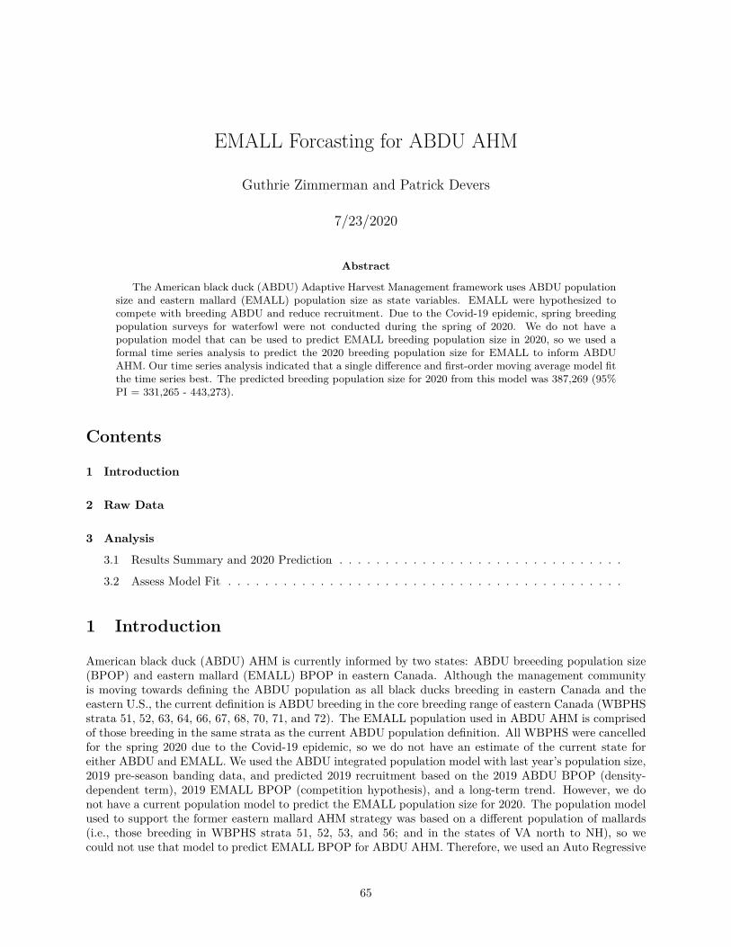
EMALL Forcasting for ABDU AHM
Guthrie Zimmerman and Patrick Devers
7/23/2020
Abstract
The American black duck (ABDU) Adaptive Harvest Management framework uses ABDU populationsize and eastern mallard (EMALL) population size as state variables. EMALL were hypothesized tocompete with breeding ABDU and reduce recruitment. Due to the Covid-19 epidemic, spring breedingpopulation surveys for waterfowl were not conducted during the spring of 2020. We do not have apopulation model that can be used to predict EMALL breeding population size in 2020, so we used aformal time series analysis to predict the 2020 breeding population size for EMALL to inform ABDUAHM. Our time series analysis indicated that a single difference and first-order moving average model fitthe time series best. The predicted breeding population size for 2020 from this model was 387,269 (95%PI = 331,265 - 443,273).
Contents
1 Introduction
2 Raw Data
3 Analysis
3.1 Results Summary and 2020 Prediction . . . . . . . . . . . . . . . . . . . . . . . . . . . . . . .
3.2 Assess Model Fit . . . . . . . . . . . . . . . . . . . . . . . . . . . . . . . . . . . . . . . . . . .
1 Introduction
American black duck (ABDU) AHM is currently informed by two states: ABDU breeeding population size(BPOP) and eastern mallard (EMALL) BPOP in eastern Canada. Although the management communityis moving towards defining the ABDU population as all black ducks breeding in eastern Canada and theeastern U.S., the current definition is ABDU breeding in the core breeding range of eastern Canada (WBPHSstrata 51, 52, 63, 64, 66, 67, 68, 70, 71, and 72). The EMALL population used in ABDU AHM is comprisedof those breeding in the same strata as the current ABDU population definition. All WBPHS were cancelledfor the spring 2020 due to the Covid-19 epidemic, so we do not have an estimate of the current state foreither ABDU and EMALL. We used the ABDU integrated population model with last year’s population size,2019 pre-season banding data, and predicted 2019 recruitment based on the 2019 ABDU BPOP (density-dependent term), 2019 EMALL BPOP (competition hypothesis), and a long-term trend. However, we donot have a current population model to predict the EMALL population size for 2020. The population modelused to support the former eastern mallard AHM strategy was based on a different population of mallards(i.e., those breeding in WBPHS strata 51, 52, 53, and 56; and in the states of VA north to NH), so wecould not use that model to predict EMALL BPOP for ABDU AHM. Therefore, we used an Auto Regressive
65

Integrated Moving Average (ARIMA) approach to predict a 2020 BPOP for EMALL based on the historictime series.
We used the ‘forecast’ package with the ARIMA function in program R as recommended by Hyndman andAthanasopoulos (2018) to identify the best approach for forecasting the 2020 EMALL population:
1. Inspect the raw data for stationarity - a stationary population is one with random fluctuations wherea count is not influenced by the time at which its observed (i.e., no trends or seasonality).
2. Use model selection (AICc) and a stepwise selection to identify the best autoregressive, differencing,or moving average (and order for each) is best for forecasting the time series based on the nature ofthe historic data.
3. Present fit tests to assess how well the selected model fits.
2 Raw Data
We explored the raw data for stationarity using:
1. Plot pf the raw data through time and simple regression of year and time to see if there is evidence ofa trend
2. Produced an Autocorrelation plot of the coefficients of correlation between a time series and lags ofthat time series. Stationary data have autocorrelation go to zero rapidly within very few time lags.
3. Conducted a Box-Ljung test, which assess the overall randomness of the data rather than autocorre-lation at specific time lags. The null hypothesis for this test is that the data represent randomness orwhite noise
4. Conducted a KPSS unit root test to assess whether differencing (i.e., use the difference between sub-sequent observations in the analysis) is likely needed to achieve stationarity. The null hypothesis isthat the data are random, so rejecting the null suggests that differencing is needed. As implementedin ARIMA, the test statistic is compared to the critical values at different levels in the output.
raw.dat <- read.csv(paste(root,’integrated.csv’,sep=’’))mall <- raw.dat[,c(’Year’,’mall_med’,’mall_se’,’mall_LCI95’,’mall_UCI95’)]# Assess stationarity
# Visualize data and run simple regression to look for trends and extreme observationsplot(mall$Year,mall$mall_med/100,type=’l’,lwd=3,xlab = ’Year’,ylab = ’EMALL BPOP (in 100,000s)’,ylim=c(0,8))
lines(mall$Year,mall$mall_LCI95/100000,lty=3,lwd=3)lines(mall$Year,mall$mall_UCI95/100000,lty=3,lwd=3)
66

1990 1995 2000 2005 2010 2015 2020
02
46
8
Year
EM
ALL
BP
OP
(in
100
,000
s)
glm.trend <- glm(mall_med ~ Year, data = mall)summary(glm.trend)
#### Call:## glm(formula = mall_med ~ Year, data = mall)#### Deviance Residuals:## Min 1Q Median 3Q Max## -58.017 -14.518 1.383 14.159 62.640#### Coefficients:## Estimate Std. Error t value Pr(>|t|)## (Intercept) -5180.5994 1164.2915 -4.450 0.000125 ***## Year 2.7752 0.5808 4.778 0.0000509 ***## ---## Signif. codes: 0 ’***’ 0.001 ’**’ 0.01 ’*’ 0.05 ’.’ 0.1 ’ ’ 1#### (Dispersion parameter for gaussian family taken to be 758.2334)#### Null deviance: 38540 on 29 degrees of freedom## Residual deviance: 21231 on 28 degrees of freedom## AIC: 288#### Number of Fisher Scoring iterations: 2
67
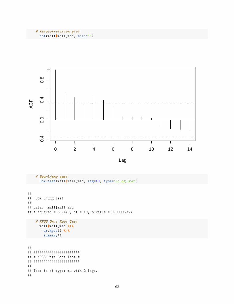
# Autocorrelation plotacf(mall$mall_med, main="")
0 2 4 6 8 10 12 14
−0.
40.
00.
40.
8
Lag
AC
F
# Box-Ljung testBox.test(mall$mall_med, lag=10, type="Ljung-Box")
#### Box-Ljung test#### data: mall$mall_med## X-squared = 36.479, df = 10, p-value = 0.00006963
# KPSS Unit Root Testmall$mall_med %>%
ur.kpss() %>%summary()
#### ######################### # KPSS Unit Root Test ### ########################### Test is of type: mu with 2 lags.##
68

## Value of test-statistic is: 0.7761#### Critical value for a significance level of:## 10pct 5pct 2.5pct 1pct## critical values 0.347 0.463 0.574 0.739
Inspection of the raw data indicated that the EMALL time series is not stationary, and that differencing islikely needed and a basic autocorrelation or random walk model might not be appropriate. The 4 checksindicated:
1. The raw data plot indicated an increasing trend over time and the simple linear regression indicated asignificant positive slope
2. The autocorrelation did not approach zero until several lags; and even went slightly negative towardsthe longest lags
3. The Box-Ljung test had a small p-value, which rejects the null hypothesis of randomness in the data4. The unit root test test-statistic was slightly greater than the significance level at 1 percent (i.e., out in
the tail), so it rejects the hypothesis of overall stationarity in the data.
3 Analysis
We used the auto.arima function to estimate the best approach and ordering for forecasting EMALL BPOPbased on the historic time series. The auto.arima function returns a vector with three elements to summarizethe results of model selection (i.e., ARIMA(x,y,z)):
1. Element x represents autoregressive models (0 = autoregressive model not appropriate, >0 = order forautoregressive model AR(1), AR(2), etc)
2. Element y represents differencing (0 = differencing not needed, >0 = order for differencing)3. Element z represents whether a moving average model is appropriate (0 = moving average model not
needed, >0 = order for moving average model)
3.1 Results Summary and 2020 Prediction
Model selection indicated ARIMA(0,1,1) indicating that differencing of 1 time step and MA(1) fit the databest. The regression was conducted on differences among years (N=29) rather than the actual annualestimates (N=30) and the values were the current and single time lag regression errors rather than thepopulation sizes. The resulting regression equation is: yt = εt − 0.6110εt−1. The εt terms in this modelare not directly observed, so this is not a standard regression and the values in the model are estimatedfrom recursive estimation. The population sizes are considered weighted moving averages of the past year’sforecast error. This model was selected at best due to the inherent trend in the time series.
## Series: dat## ARIMA(0,1,1)#### Coefficients:## ma1## -0.6110## s.e. 0.1402#### sigma^2 estimated as 816.5: log likelihood=-138.1## AIC=280.19 AICc=280.65 BIC=282.93
69

Table 1: Predicted BPOP for EMALL (and prediction intervals) for 2020
Point Forecast Lo 80 Hi 80 Lo 95 Hi 952020 387.2688 350.6497 423.8879 331.2647 443.2729
0
100
200
300
400
500
1990 2000 2010 2020Year: 1990−2020
EM
ALL
BP
OP
(in
1,0
00s)
Observed (black) and predicted (blue) EMALL BPOP
3.2 Assess Model Fit
Inspection of model fit indicated that ARIMA(0,1,1) model adequately fit the time series. The Ljung-Box testhad a p-value of 0.328, so we do not reject the null hypothesis of random variation and the autocorrelationplot centered around zero within acceptable limits (dotted blue lines in the ACF plot below). Althoughoverall, the model appeared to fit well, the residual plots indicated some lack of fit. The time series ofresidual plot indicated a slight declining trend and the residual histogram was slightly left-skewed. Themean of the residuals should ideally be zero (equally under and over fit), but the mean of the residuals wasabout 6. This pattern indicated that early in the time series the model slightly over-predicted, whereas laterin the time series, the model slightly under-predicted. This is likely due to the trend in the raw data wherethe population was increasing until a certain point where it appears to stabilize or slightly decrease.
70

−40
0
40
1990 1995 2000 2005 2010 2015 2020
Residuals from ARIMA(0,1,1)
−0.2
0.0
0.2
1 2 3 4 5 6 7 8 9 10Lag
AC
F
0
3
6
9
−100 −50 0 50 100residuals
coun
t
#### Ljung-Box test#### data: Residuals from ARIMA(0,1,1)## Q* = 5.7823, df = 5, p-value = 0.328#### Model df: 1. Total lags used: 6
71

Northern Pintail AHM - Latitude Forecast:Spring 2020
G. Scott Boomer
Branch of Assessment and Decision SupportDivision of Migratory Bird Management
U.S. Fish and Wildlife [email protected]
20 August 2020
Abstract
Due to the COVID-19 pandemic, waterfowl breeding populations were not directly observedin the spring of 2020. As a result, waterfowl harvest regulations will have to be informedwith information based on predictions of breeding population sizes and habitat conditions. Wedeveloped an estimation and forecasting framework to predict the distribution (weighted latitude)of the pintail (Anas acuta) breeding population in the spring of 2020 based on historical breedingdistribution information from 1980–2019. We used an autoregressive integrated moving average(ARIMA) estimation framework to develop a model to forecast the breeding distribution of pintailsin 2020. A 1st order autoregressive model [ARIMA (1,0,0)] was best supported by the data. Basedon our selected model, the forecast of the latitude of the 2020 pintail breeding population is 55.16degrees (95% PI = 51.78 – 58.55).
ContentsBackground . . . . . . . . . . . . . . . . . . . . . . . . . . . . . . . . . . . . . . . . . . . . .
Latitude Time Series Analysis . . . . . . . . . . . . . . . . . . . . . . . . . . . . . . . . . .
Data . . . . . . . . . . . . . . . . . . . . . . . . . . . . . . . . . . . . . . . . . . . . . . . . . .
2020 Pintail Latitude Forecast . . . . . . . . . . . . . . . . . . . . . . . . . . . . . . . . . .
References . . . . . . . . . . . . . . . . . . . . . . . . . . . . . . . . . . . . . . . . . . . . . .
72

List of Tables
List of Figures1 The observed latitude of the pintail breeding population distribution from 1980–2019.2 Residual diagnostics from the selected model [ARIMA (1,0,0)]. . . . . . . . . . . . .3 The 2020 forecast of the latitude of the pintail breeding population distribution. . .
73

BackgroundDue to the COVID-19 pandemic, the United States Fish and Wildlife Service (USFWS) and its partnerswere unable to conduct the Waterfowl Breeding Population and Habitat Survey (WBPHS) to estimatethe 2020 waterfowl breeding populations as well as evaluate breeding habitat conditions. As a result,the promulgation of waterfowl harvest regulations in 2020 will require some modi�cations to thedecision protocols that typically govern the regulatory process. In the absence of this information,the USFWS proposes to base 2020 regulatory decisions on predictions of breeding population sizesand habitat conditions. Current system models for which we have AHM decision frameworks willbe used to predict 2020 population sizes based on the breeding population sizes, habitat conditions,harvest, and harvest rates observed in 2019. However, several harvest strategies such as pintail AHMrely on other forms of information (e.g., breeding distribution) to establish decision thresholds. As aresult, we developed an estimation framework to forecast the latitude of the 2020 pintail breedingpopulation distribution.
Latitude Time Series Analysis
Data
nopi_dat<-getBPOP.fn(1430,"MAS",1980:2019,1e6)# bind data into a time series object for convenience
lat_ts<-ts(nopi_dat$lat,frequency=1,start=1980,end=2019)
We are interested in predicting the 2020 pintail breeding distribution (weighted latitude) from thehistorical time series of breeding population estimates. We summarized breeding ground distributioninformation in the form of a BPOP weighted average of the latitude of the centroid of each strata inthe traditional survey area of the Waterfowl Breeding Population and Habitat Survey (U.S. Fish andWildlife Service 2019). Based on previous analyses that documented a temporal shift in the distributionof breeding pintails (Runge and Boomer 2005, M. C. Runge USGS, personal communication), werestricted our analyses to information from 1980–2019 (Figure 1).
74
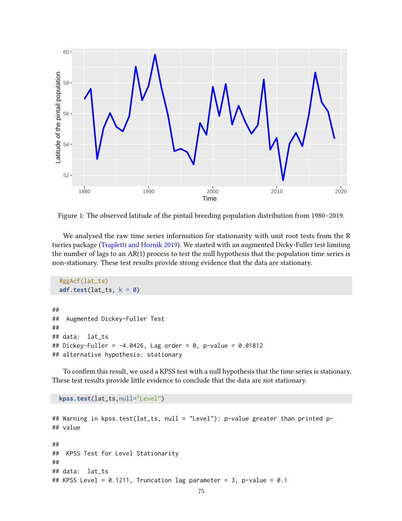
52
54
56
58
60
1980 1990 2000 2010 2020Time
Latit
ude
of th
e pi
ntai
l pop
ulat
ion
Figure 1: The observed latitude of the pintail breeding population distribution from 1980–2019.
We analysed the raw time series information for stationarity with unit root tests from the Rtseries package (Trapletti and Hornik 2019). We started with an augmented Dicky-Fuller test limitingthe number of lags to an AR(1) process to test the null hypothesis that the population time series isnon-stationary. These test results provide strong evidence that the data are stationary.
#ggAcf(lat_ts)
adf.test(lat_ts, k = 0)
##
## Augmented Dickey-Fuller Test
##
## data: lat_ts
## Dickey-Fuller = -4.0426, Lag order = 0, p-value = 0.01812
## alternative hypothesis: stationary
To con�rm this result, we used a KPSS test with a null hypothesis that the time series is stationary.These test results provide little evidence to conclude that the data are not stationary.
kpss.test(lat_ts,null="Level")
## Warning in kpss.test(lat_ts, null = "Level"): p-value greater than printed p-
## value
##
## KPSS Test for Level Stationarity
##
## data: lat_ts
## KPSS Level = 0.1211, Truncation lag parameter = 3, p-value = 0.1
75

We analysed the historical information with an autoregressive integrated moving average (ARIMA)estimation framework, using the auto.arima function from the Forecast R package (Hyndman et al.2020, Hyndman and Khandakar 2008) to determine the appropriate number of lags and di�erencing(Hyndman and Athanasopoulos 2018) for the �nal speci�cation of our ARIMA model.
fit_lat<-auto.arima(lat_ts,stepwise=FALSE,approximation=FALSE,trace=TRUE)
##
## ARIMA(0,0,0) with zero mean : 437.1984
## ARIMA(0,0,0) with non-zero mean : 165.9492
## ARIMA(0,0,1) with zero mean : Inf
## ARIMA(0,0,1) with non-zero mean : 163.692
## ARIMA(0,0,2) with zero mean : Inf
## ARIMA(0,0,2) with non-zero mean : 163.2817
## ARIMA(0,0,3) with zero mean : Inf
## ARIMA(0,0,3) with non-zero mean : 165.7076
## ARIMA(0,0,4) with zero mean : Inf
## ARIMA(0,0,4) with non-zero mean : 165.9126
## ARIMA(0,0,5) with zero mean : Inf
## ARIMA(0,0,5) with non-zero mean : 168.7623
## ARIMA(1,0,0) with zero mean : Inf
## ARIMA(1,0,0) with non-zero mean : 161.9086
## ARIMA(1,0,1) with zero mean : Inf
## ARIMA(1,0,1) with non-zero mean : 164.2008
## ARIMA(1,0,2) with zero mean : Inf
## ARIMA(1,0,2) with non-zero mean : 165.6069
## ARIMA(1,0,3) with zero mean : Inf
## ARIMA(1,0,3) with non-zero mean : 169.0239
## ARIMA(1,0,4) with zero mean : Inf
## ARIMA(1,0,4) with non-zero mean : 168.8571
## ARIMA(2,0,0) with zero mean : Inf
## ARIMA(2,0,0) with non-zero mean : 164.0091
## ARIMA(2,0,1) with zero mean : Inf
## ARIMA(2,0,1) with non-zero mean : 165.1546
## ARIMA(2,0,2) with zero mean : Inf
## ARIMA(2,0,2) with non-zero mean : 167.9224
## ARIMA(2,0,3) with zero mean : Inf
## ARIMA(2,0,3) with non-zero mean : Inf
## ARIMA(3,0,0) with zero mean : Inf
## ARIMA(3,0,0) with non-zero mean : 165.1493
## ARIMA(3,0,1) with zero mean : Inf
## ARIMA(3,0,1) with non-zero mean : 165.0755
## ARIMA(3,0,2) with zero mean : Inf
## ARIMA(3,0,2) with non-zero mean : Inf
## ARIMA(4,0,0) with zero mean : Inf
## ARIMA(4,0,0) with non-zero mean : 167.4134
## ARIMA(4,0,1) with zero mean : Inf
## ARIMA(4,0,1) with non-zero mean : 167.8004
## ARIMA(5,0,0) with zero mean : Inf
## ARIMA(5,0,0) with non-zero mean : 166.1395
76

##
##
##
## Best model: ARIMA(1,0,0) with non-zero mean
summary(fit_lat)
## Series: lat_ts
## ARIMA(1,0,0) with non-zero mean
##
## Coefficients:
## ar1 mean
## 0.3836 55.6559
## s.e. 0.1450 0.4248
##
## sigma^2 estimated as 2.976: log likelihood=-77.62
## AIC=161.24 AICc=161.91 BIC=166.31
##
## Training set error measures:
## ME RMSE MAE MPE MAPE MASE
## Training set -0.01472947 1.681347 1.312912 -0.1177028 2.357408 0.7654633
## ACF1
## Training set -0.03108714
print(fit_lat)
## Series: lat_ts
## ARIMA(1,0,0) with non-zero mean
##
## Coefficients:
## ar1 mean
## 0.3836 55.6559
## s.e. 0.1450 0.4248
##
## sigma^2 estimated as 2.976: log likelihood=-77.62
## AIC=161.24 AICc=161.91 BIC=166.31
#checkresiduals(fit_lat)
77

−2
0
2
1980 1990 2000 2010 2020
Residuals from ARIMA(1,0,0) with non−zero mean
−0.2
0.0
0.2
1 2 3 4 5 6 7 8 9 10 11 12 13Lag
AC
F
0
5
10
−6 −3 0 3 6residuals
coun
t
Figure 2: Residual diagnostics from the selected model [ARIMA (1,0,0)].
##
## Ljung-Box test
##
## data: Residuals from ARIMA(1,0,0) with non-zero mean
## Q* = 10.665, df = 6, p-value = 0.09931
##
## Model df: 2. Total lags used: 8
2020 Pintail Latitude ForecastThe model selection results suggest that a 1st order autoregressive model [ARIMA (1,0,0)] is bestsupported by the data. Model diagnostics indicate that the residuals are uncorrelated and the selectedmodel does not show a lack of �t (Figure 2). We can use these model results to forecast the distributionof the pintail breeding population in 2020.
lat_2020 <- forecast(fit_lat,h=1)summary(lat_2020)
##
## Forecast method: ARIMA(1,0,0) with non-zero mean
##
## Model Information:
## Series: lat_ts78
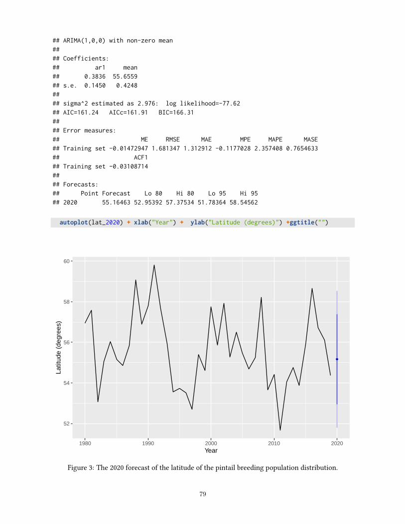
## ARIMA(1,0,0) with non-zero mean
##
## Coefficients:
## ar1 mean
## 0.3836 55.6559
## s.e. 0.1450 0.4248
##
## sigma^2 estimated as 2.976: log likelihood=-77.62
## AIC=161.24 AICc=161.91 BIC=166.31
##
## Error measures:
## ME RMSE MAE MPE MAPE MASE
## Training set -0.01472947 1.681347 1.312912 -0.1177028 2.357408 0.7654633
## ACF1
## Training set -0.03108714
##
## Forecasts:
## Point Forecast Lo 80 Hi 80 Lo 95 Hi 95
## 2020 55.16463 52.95392 57.37534 51.78364 58.54562
autoplot(lat_2020) + xlab("Year") + ylab("Latitude (degrees)") +ggtitle("")
52
54
56
58
60
1980 1990 2000 2010 2020Year
Latit
ude
(deg
rees
)
Figure 3: The 2020 forecast of the latitude of the pintail breeding population distribution.
79

lat_2020_sd<-(lat_2020$upper[,1] - lat_2020$lower[,1]) /(2 * qnorm(.5 + lat_2020$level[1] / 200))
mean_abs <- format(round(as.numeric(lat_2020$mean),2),nsmall=2)upper_abs<-format(round(lat_2020$upper[2],2),nsmall=2)lower_abs<-format(round(lat_2020$lower[2],2),nsmall=2)print(paste("SD =",round(lat_2020_sd,3),sep=""))
## [1] "SD =1.725"
Based on the selected model, the forecast for the latitude of the 2020 pintail breeding populationis 55.16 degrees with a 95% prediction interval ranging from 51.78 to 58.55 (Figure 3).
ReferencesHyndman, R., and G. Athanasopoulos. 2018. Forecasting: principles and practice, 2nd edition. OTexts:
Melbourne, Melbourne, Australia.
Hyndman, R., G. Athanasopoulos, C. Bergmeir, G. Caceres, L. Chhay, M. O’Hara-Wild, F. Petropoulos,S. Razbash, E. Wang, and F. Yasmeen. 2020. forecast: Forecasting functions for time series andlinear models. R package version 8.12. URL http://pkg.robjhyndman.com/forecast.
Hyndman, R. J., and Y. Khandakar. 2008. Automatic time series forecasting: the forecast package for R.Journal of Statistical Software 26:1–22. URL http://www.jstatsoft.org/article/view/v027i03.
Runge, M. C., and G. S. Boomer, 2005. Population dynamics and harvest management of the continentalnorthern pintail population. Unpublished Report. U.S. Geological Survey, Patuxent WildlifeResearch Center, Laurel, MD. 42pp.
Trapletti, A., and K. Hornik. 2019. tseries: Time Series Analysis and Computational Finance. Rpackage version 0.10-47. URL https://CRAN.R-project.org/package=tseries.
U.S. Fish and Wildlife Service, 2019. Waterfowl population status, 2019. U.S. Department of In-terior, Washington, D.C., URL https://www.fws.gov/migratorybirds/pdf/surveys-and-data/
Population-status/Waterfowl/WaterfowlPopulationStatusReport19.pdf.
80

Appendix H Mid-Continent Mallard Models
In 1995, we developed population models to predict changes in mid-continent mallards based on the traditionalsurvey area which includes individuals from Alaska (Johnson et al. 1997). In 1997, we added mallards fromthe Great Lakes region (Michigan, Minnesota, and Wisconsin) to the mid-continent mallard stock, assumingtheir population dynamics were equivalent. In 2002, we made extensive revisions to the set of alternativemodels describing the population dynamics of mid-continent mallards (Runge et al. 2002, U.S. Fish andWildlife Service 2002). In 2008, we redefined the population of mid-continent mallards Table H.1 to accountfor the removal of Alaskan birds (WBPHS strata 1–12) that are now considered to be in the western mallardstock and have subsequently rescaled the model set accordingly.
Table H.1 – Estimates (N) and associated standard errors (SE) of mid-continent mallards (in millions) observedin the WBPHS (strata 13–18, 20–50, and 75–77) and the Great Lakes region (Michigan, Minnesota, and Wis-consin) from 1992 to 2019. The waterfowl breeding population surveys were not conducted in 2020 due to theCOVID-19 pandemic; 2020 numbers are based on model predictions.
WBPHS area Great Lakes region Total
Year N SE N SE N SE
1992 5.6304 0.2379 0.9964 0.1178 6.6267 0.2654
1993 5.4253 0.2068 0.9176 0.0827 6.3429 0.2227
1994 6.6292 0.2803 1.1304 0.1153 7.7596 0.3031
1995 7.7452 0.2793 1.0857 0.1323 8.8309 0.3090
1996 7.4193 0.2593 1.0074 0.0991 8.4267 0.2776
1997 9.3554 0.3041 1.0777 0.1140 10.4332 0.3248
1998 8.8041 0.2940 1.0783 0.1172 9.8825 0.3165
1999 10.0926 0.3374 1.0309 0.1282 11.1236 0.3610
2000 8.6999 0.2855 1.1993 0.1221 9.8992 0.3105
2001 7.1857 0.2204 0.8282 0.0718 8.0139 0.2318
2002 6.8364 0.2412 1.0684 0.0883 7.9047 0.2569
2003 7.1062 0.2589 0.8407 0.0647 7.9470 0.2668
2004 6.6142 0.2746 0.9465 0.0915 7.5607 0.2895
2005 6.0521 0.2754 0.8138 0.0677 6.8660 0.2836
2006 6.7607 0.2187 0.6249 0.0577 7.3856 0.2262
2007 7.7258 0.2805 0.7904 0.0752 8.5162 0.2904
2008 7.1914 0.2525 0.6865 0.0550 7.8779 0.2584
2009 8.0094 0.2442 0.6958 0.0625 8.7052 0.2521
2010 7.8246 0.2799 0.7793 0.0714 8.6039 0.2889
2011 8.7668 0.2650 0.7298 0.0720 9.4965 0.2746
2012 10.0959 0.3199 0.8612 0.1769 10.9571 0.3655
2013 10.0335 0.3586 0.7628 0.0744 10.7963 0.3662
2014 10.3989 0.3429 0.6459 0.0681 11.0448 0.3496
2015 11.1724 0.3582 0.6202 0.0514 11.7926 0.3619
2016 11.2083 0.3615 0.6925 0.0707 11.9008 0.3684
2017 9.9500 0.3298 0.6927 0.0523 10.6427 0.3339
2018 8.8044 0.2955 0.7634 0.0702 9.5678 0.3037
2019 9.0624 0.2823 0.6698 0.0679 9.7322 0.2903
2020 8.3372 1.4270 0.7310 0.1178 9.0681 1.4318
81

Model Structure
Collectively, the models express uncertainty (or disagreement) about whether harvest is an additive or com-pensatory form of mortality (Burnham et al. 1984), and whether the reproductive process is weakly or stronglydensity-dependent (i.e., the degree to which reproductive rates decline with increasing population size).
All population models for mid-continent mallards share a common “balance equation” to predict changes inbreeding-population size as a function of annual survival and reproductive rates:
𝑁𝑡+1 = 𝑁𝑡 (𝑚𝑆𝑡,𝐴𝑀 + (1−𝑚)(𝑆𝑡,𝐴𝐹 +𝑅𝑡(𝑆𝑡,𝐽𝐹 + 𝑆𝑡,𝐽𝑀𝜑𝑠𝑢𝑚𝐹 /𝜑𝑠𝑢𝑚
𝑀 )))
where:
N=breeding population size,
m = proportion of males in the breeding population,
𝑆𝐴𝑀 , 𝑆𝐴𝐹 , 𝑆𝐽𝐹 , and 𝑆𝐽𝑀 = survival rates of adult males, adult females, young females, and youngmales, respectively,
R = reproductive rate, defined as the fall age ratio of females,
𝜑𝑠𝑢𝑚𝐹 /𝜑𝑠𝑢𝑚
𝑀 = the ratio of female (F ) to male (M ) summer survival, and t = year.
We assumed that m and 𝜑𝑠𝑢𝑚𝐹 /𝜑𝑠𝑢𝑚
𝑀 are fixed and known. We also assumed, based in part on informationprovided by Blohm et al. (1987), the ratio of female to male summer survival was equivalent to the ratio ofannual survival rates in the absence of harvest. Based on this assumption, we estimated 𝜑𝑠𝑢𝑚
𝐹 /𝜑𝑠𝑢𝑚𝑀 = 0.897.
To estimate m we expressed the balance equation in matrix form:
[𝑁𝑡+1,𝐴𝑀
𝑁𝑡+1,𝐴𝐹
]=
[𝑆𝐴𝑀 𝑅𝑆𝐽𝑀𝜑𝑠𝑢𝑚
𝐹 /𝜑𝑠𝑢𝑚𝑀
0 𝑆𝐴𝐹 +𝑅𝑆𝐽𝐹
] [𝑁𝑡,𝐴𝑀
𝑁𝑡,𝐴𝐹
]
and substituted the constant ratio of summer survival and means of estimated survival and reproductiverates. The right eigenvector of the transition matrix is the stable sex structure that the breeding populationeventually would attain with these constant demographic rates. This eigenvector yielded an estimate ofm = 0.5246.
Using estimates of annual survival and reproductive rates, the balance equation for mid-continent mallardsover-predicted observed population sizes by 11.0% on average. The source of the bias is unknown, so wemodified the balance equation to eliminate the bias by adjusting both survival and reproductive rates:
𝑁𝑡+1 = 𝛾𝑆𝑁𝑡 (𝑚𝑆𝑡,𝑎𝑚 + (1−𝑚) (𝑆𝑡,𝐴𝐹 + 𝛾𝑅𝑅𝑡 (𝑆𝑡,𝐽𝐹 + 𝑆𝑡,𝐽𝑀𝜑𝑠𝑢𝑚𝐹 /𝜑𝑠𝑢𝑚
𝑀 )))
where 𝛾 denotes the bias-correction factors for survival (S), and reproduction (R). We used a least squaresapproach to estimate 𝛾𝑆 = 0.9407 and 𝛾𝑅 = 0.8647.
Survival Process
We considered two alternative hypotheses for the relationship between annual survival and harvest rates. Forboth models, we assumed that survival in the absence of harvest was the same for adults and young of thesame sex. In the model where harvest mortality is additive to natural mortality:
𝑆𝑡,𝑠𝑒𝑥,𝑎𝑔𝑒 = 𝑆𝐴0,𝑠𝑒𝑥(1−𝐾𝑡,𝑠𝑒𝑥,𝑎𝑔𝑒)
82

and in the model where changes in natural mortality compensate for harvest losses (up to some threshold):
𝑆𝑡,𝑠𝑒𝑥,𝑎𝑔𝑒 =
{𝑠𝐶0,𝑠𝑒𝑥 𝑖𝑓 𝐾𝑡,𝑠𝑒𝑥,𝑎𝑔𝑒 ≤ 1− 𝑠𝐶0,𝑠𝑒𝑥
1−𝐾𝑡,𝑠𝑒𝑥,𝑎𝑔𝑒 𝑖𝑓 𝐾𝑡,𝑠𝑒𝑥,𝑎𝑔𝑒 > 1− 𝑠𝐶0,𝑠𝑒𝑥
where 𝑠0 = survival in the absence of harvest under the additive (A) or compensatory (C ) model, and K =harvest rate adjusted for crippling loss (20%, Anderson and Burnham 1976). We averaged estimates of 𝑠0across banding reference areas by weighting by breeding-population size. For the additive model, 𝑠0 = 0.7896and 0.6886 for males and females, respectively. For the compensatory model, 𝑠0 = 0.6467 and 0.5965 formales and females, respectively. These estimates may seem counterintuitive because survival in the absenceof harvest should be the same for both models. However, estimating a common (but still sex-specific) 𝑠0for both models leads to alternative models that do not fit available band-recovery data equally well. Moreimportantly, it suggests that the greatest uncertainty about survival rates is when harvest rate is within therealm of experience. By allowing 𝑠0 to differ between additive and compensatory models, we acknowledgethat the greatest uncertainty about survival rate is its value in the absence of harvest (i.e., where we have noexperience).
Reproductive Process
Annual reproductive rates were estimated from age ratios in the harvest of females, corrected using a constantestimate of differential vulnerability. Predictor variables were the number of ponds in May in Prairie Canada(P, in millions) and the size of the breeding population (N, in millions). We estimated the best-fitting linearmodel, and then calculated the 80% confidence ellipsoid for all model parameters. We chose the two pointson this ellipsoid with the largest and smallest values for the effect of breeding-population size, and generateda weakly density-dependent model:
𝑅𝑡 = 0.7166 + 0.1083𝑃𝑡 − 0.0373𝑁𝑡
and a strongly density-dependent model:
𝑅𝑡 = 1.1390 + 0.1376𝑃𝑡 − 0.1131𝑁𝑡
Predicted recruitment was then rescaled to reflect the current definition of mid-continent mallards which nowexcludes birds from Alaska but includes mallards observed in the Great Lakes region.
Pond Dynamics
Wemodeled annual variation in Canadian pond numbers as a first-order autoregressive process. The estimatedmodel was:
𝑃𝑡+1 = 2.2127 + 0.3420𝑃𝑡 + 𝜀𝑡
where ponds are in millions and 𝜀𝑡 is normally distributed with mean = 0 and variance = 1.2567.
83

Variance of Prediction Errors
Using the balance equation and sub-models described above, predictions of breeding-population size in yeart+1 depend only on specification of population size, pond numbers, and harvest rate in year t. For the periodin which comparisons were possible, we compared these predictions with observed population sizes.
We estimated the prediction-error variance by setting:
𝑒𝑡 = ln(𝑁𝑜𝑏𝑠
𝑡
)− ln (𝑁𝑝𝑟𝑒
𝑡 )
𝑒𝑡 ∼ 𝑁(0, 𝜎2
)𝜎2 =
∑𝑡
[ln(𝑁𝑜𝑏𝑠
𝑡
)− ln (𝑁𝑝𝑟𝑒
𝑡 )]2
/(𝑛− 1)
where 𝑁𝑜𝑏𝑠 and 𝑁𝑝𝑟𝑒 are observed and predicted population sizes (in millions), respectively, and n = thenumber of years being compared. We were concerned about a variance estimate that was too small, eitherby chance or because the number of years in which comparisons were possible was small. Therefore, wecalculated the upper 80% confidence limit for 𝜎2 based on a Chi-squared distribution for each combinationof the alternative survival and reproductive sub-models, and then averaged them. The final estimate of 𝜎2
was 0.0280, equivalent to a coefficient of variation of about 16.85%.
Model Implications
The population model with additive hunting mortality and weakly density-dependent recruitment (SaRw)leads to the most conservative harvest strategy, whereas the model with compensatory hunting mortalityand strongly density-dependent recruitment (ScRs) leads to the most liberal strategy. The other two models(SaRs and ScRw) lead to strategies that are intermediate between these extremes. Under the models withcompensatory hunting mortality (ScRs and ScRw), the optimal strategy is to have a liberal regulation re-gardless of population size or number of ponds because at harvest rates achieved under the liberal alternative,harvest has no effect on population size. Under the strongly density-dependent model (ScRs), the densitydependence regulates the population and keeps it within narrow bounds. Under the weakly density dependentmodel (ScRw), the density-dependence does not exert as strong a regulatory effect, and the population sizefluctuates more.
Model Weights
Model weights are calculated as Bayesian probabilities, reflecting the relative ability of the individual alter-native models to predict observed changes in population size. The Bayesian probability for each model is afunction of the model’s previous (or prior) weight and the likelihood of the observed population size underthat model. We used Bayes’ theorem to calculate model weights from a comparison of predicted and observedpopulation sizes for the years 1996–2019, starting with equal model weights in 1995.
84
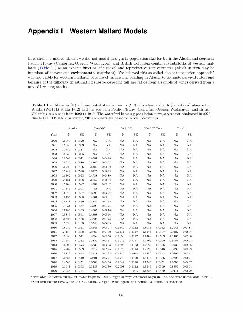
Appendix I Western Mallard Models
In contrast to mid-continent, we did not model changes in population size for both the Alaska and southernPacific Flyway (California, Oregon, Washington, and British Columbia combined) substocks of western mal-lards (Table I.1) as an explicit function of survival and reproductive rate estimates (which in turn may befunctions of harvest and environmental covariates). We believed this so-called “balance-equation approach”was not viable for western mallards because of insufficient banding in Alaska to estimate survival rates, andbecause of the difficulty in estimating substock-specific fall age ratios from a sample of wings derived from amix of breeding stocks.
Table I.1 – Estimates (N) and associated standard errors (SE) of western mallards (in millions) observed inAlaska (WBPHS strata 1–12) and the southern Pacific Flyway (California, Oregon, Washington, and BritishColumbia combined) from 1990 to 2019. The waterfowl breeding population surveys were not conducted in 2020due to the COVID-19 pandemic; 2020 numbers are based on model predictions.
Alaska CA-ORa WA-BC SO–PFb Total Total
Year N SE N SE N SE N SE N SE
1990 0.3669 0.0370 NA NA NA NA NA NA NA NA
1991 0.3853 0.0363 NA NA NA NA NA NA NA NA
1992 0.3457 0.0387 NA NA NA NA NA NA NA NA
1993 0.2830 0.0295 NA NA NA NA NA NA NA NA
1994 0.3509 0.0371 0.4281 0.0425 NA NA NA NA NA NA
1995 0.5242 0.0680 0.4460 0.0427 NA NA NA NA NA NA
1996 0.5220 0.0436 0.6389 0.0802 NA NA NA NA NA NA
1997 0.5842 0.0520 0.6325 0.1043 NA NA NA NA NA NA
1998 0.8362 0.0673 0.4788 0.0489 NA NA NA NA NA NA
1999 0.7131 0.0696 0.6857 0.1066 NA NA NA NA NA NA
2000 0.7703 0.0522 0.4584 0.0532 NA NA NA NA NA NA
2001 0.7183 0.0541 NA NA NA NA NA NA NA NA
2002 0.6673 0.0507 0.3698 0.0327 NA NA NA NA NA NA
2003 0.8435 0.0668 0.4261 0.0501 NA NA NA NA NA NA
2004 0.8111 0.0639 0.3449 0.0352 NA NA NA NA NA NA
2005 0.7031 0.0547 0.3920 0.0474 NA NA NA NA NA NA
2006 0.5158 0.0469 0.4805 0.0576 NA NA NA NA NA NA
2007 0.5815 0.0551 0.4808 0.0546 NA NA NA NA NA NA
2008 0.5324 0.0468 0.3725 0.0478 NA NA NA NA NA NA
2009 0.5030 0.0449 0.3746 0.0639 NA NA NA NA NA NA
2010 0.6056 0.0531 0.4347 0.0557 0.1740 0.0132 0.6087 0.0572 1.2143 0.0781
2011 0.4158 0.0388 0.3763 0.0452 0.1411 0.0117 0.5174 0.0467 0.9332 0.0607
2012 0.5056 0.0511 0.4759 0.0550 0.1650 0.0117 0.6409 0.0563 1.1465 0.0760
2013 0.3384 0.0382 0.3830 0.0527 0.1573 0.0117 0.5403 0.0540 0.8787 0.0661
2014 0.5009 0.0574 0.3239 0.0553 0.1690 0.0123 0.4929 0.0566 0.9938 0.0806
2015 0.4709 0.0509 0.2612 0.0295 0.1678 0.0114 0.4290 0.0316 0.8999 0.0599
2016 0.5842 0.0654 0.3511 0.0365 0.1339 0.0078 0.4850 0.0373 1.0692 0.0753
2017 0.5385 0.0519 0.2701 0.0324 0.1743 0.0120 0.4444 0.0346 0.9828 0.0624
2018 0.4508 0.0451 0.3700 0.0436 0.2042 0.0115 0.5743 0.0451 1.0250 0.0637
2019 0.3611 0.0353 0.3237 0.0330 0.2008 0.0142 0.5245 0.0359 0.8855 0.0504
2020 0.4086 0.0731 NA NA NA NA 0.5325 0.0559 0.9411 0.0920
a Available California survey estimates begin in 1992; Oregon surveys estimates begin in 1994 and were unavailable in 2001.b Southern Pacific Flyway includes California, Oregon, Washington, and British Columbia observations.
85

Model Structure
To evaluate western mallard population dynamics, we used a discrete logistic model (Schaefer 1954), whichcombines reproduction and natural mortality into a single parameter r, the intrinsic rate of growth. Themodel assumes density-dependent growth, which is regulated by the ratio of population size, N, to thecarrying capacity of the environment, K (i.e., equilibrium population size in the absence of harvest). Inthe traditional formulation, harvest mortality is additive to other sources of mortality, but compensation forhunting losses can occur through subsequent increases in production. However, we parameterized the modelin a way that also allows for compensation of harvest mortality between the hunting and breeding seasons.It is important to note that compensation modeled in this way is purely phenomenological, in the sensethat there is no explicit ecological mechanism for compensation (e.g., density-dependent mortality after thehunting season). The basic model for both the Alaska and southern Pacific Flyway substocks has the form:
𝑁𝑡+1 =
[𝑁𝑡 +𝑁𝑡𝑟
(1− 𝑁𝑡
𝐾
)](1− 𝛼𝑡)
where,
𝛼𝑡 = 𝑑ℎ𝐴𝑀𝑡
and where t = year, ℎ𝐴𝑀 = the harvest rate of adult males, and d = a scaling factor. The scaling factor isused to account for a combination of unobservable effects, including un-retrieved harvest (i.e., crippling loss),differential harvest mortality of cohorts other than adult males, and for the possibility that some harvestmortality may not affect subsequent breeding-population size (i.e., the compensatory mortality hypothesis).
Estimation Framework
We used Bayesian estimation methods in combination with a state-space model that accounts explicitly forboth process and observation error in breeding population size. This combination of methods is becomingwidely used in natural resource modeling, in part because it facilitates the fitting of non-linear models thatmay have non-normal errors (Meyer and Millar 1999). The Bayesian approach also provides a natural andintuitive way to portray uncertainty, allows one to incorporate prior information about model parameters, andpermits the updating of parameter estimates as further information becomes available. Breeding populationdata are available for California and Oregon from 1994–2019 (except for 2001), British Columbia from 2006–2019, and Washington from 2010–2019 (see Table I.1). We attempted to use correlations with adjacent statesto impute data back to 1992 for WA and BC, but could not find a reasonable correlation between those surveysand other regions (potentially due to a short time series). Therefore, we imputed population estimates forBC and WA by sampling values from the mean and variance within the MCMC framework. Specifically, wecalculated the total mean and variance of breeding population sizes based on observed data (2006–2019 forBritish Columbia, and 2010–2019 for Washington), and then used those means and variances to sample apopulation size for the missing years (1992–2005 for British Columbia; and 1992–2009 for Washington) duringeach iteration of MCMC sampling. Although this approach imputes values based on a random draw, it doesacknowledge added uncertainty in those estimates compared to the years with observed data. Further, giventhe low annual variability and lack of trend, we have no evidence that the recent survey estimates used togenerate the mean and variance are not a reasonable approximation of historical breeding population sizes.
We first scaled N by K as recommended by Meyer and Millar (1999), and assumed that process errors werelognormally distributed with mean 0 and variance 𝜎2. Thus, the process model had the form:
𝑃𝑡 = 𝑁𝑡/𝐾
log(𝑃𝑡) = log([𝑃𝑡−1 + 𝑃𝑡−1𝑟 (1− 𝑃𝑡−1)]
(1− 𝑑ℎ𝐴𝑀
𝑡−1
))+ 𝑒𝑡
86

where,
𝑒𝑡 ∼ 𝑁(0, 𝜎2)
The observation model related the unknown population sizes (𝑃𝑡𝐾) to the population sizes (𝑁𝑡) estimatedfrom the breeding-population surveys in Alaska and southern Pacific Flyway. We assumed that the observa-tion process yielded additive, normally distributed errors, which were represented by:
𝑁𝑡 = 𝑃𝑡𝐾 + 𝜀𝐵𝑃𝑂𝑃𝑡 ,
where,
𝜀𝐵𝑃𝑂𝑃𝑡 ∼ 𝑁(0, 𝜎2
𝐵𝑃𝑂𝑃 ).
permitting us to estimate the process error, which reflects the inability of the model to completely describechanges in population size. The process error reflects the combined effect of misspecification of an appropriatemodel form, as well as any un-modeled environmental drivers. We initially examined a number of possibleenvironmental covariates, including the Palmer Drought Index in California and Oregon, spring temperaturein Alaska, and the El Nino Southern Oscillation Index (http://www.cdc.noaa.gov/people/klaus.wolter/MEI/mei.html). While the estimated effects of these covariates on r or K were generally what one would expect,they were never of sufficient magnitude to have a meaningful effect on optimal harvest strategies. We thereforechose not to further pursue an investigation of environmental covariates, and posited that the process errorwas a sufficient surrogate for these un-modeled effects. Parameterization of the models also required measuresof harvest rate. Beginning in 2002, harvest rates of adult males were estimated directly from the recovery ofreward bands. Prior to 1993, we used direct recoveries of standard bands, corrected for band-reporting ratesprovided by Nichols et al. (1995b). We also used the band-reporting rates provided by Nichols et al. (1995b)for estimating harvest rates in 1994 and 1995, except that we inflated the reporting rates of full-addressand toll-free bands based on an unpublished analysis by Clint Moore and Jim Nichols (Patuxent WildlifeResearch Center). We were unwilling to estimate harvest rates for the years 1996–2001 because of suspected,but unknown, increases in the reporting rates of all bands. For simplicity, harvest rate estimates were treatedas known values in our analysis, although future analyses might benefit from an appropriate observationmodel for these data.
In a Bayesian analysis, one is interested in making probabilistic statements about the model parameters(𝜃), conditioned on the observed data. Thus, we are interested in evaluating 𝑃 (𝜃|𝑑𝑎𝑡𝑎), which requiresthe specification of prior distributions for all model parameters and unobserved system states (𝜃) and thesampling distribution (likelihood) of the observed data 𝑃 (𝑑𝑎𝑡𝑎|𝜃). Using Bayes theorem, we can representthe posterior probability distribution of model parameters, conditioned on the data, as:
𝑃 (𝜃|𝑑𝑎𝑡𝑎) ∝ 𝑃 (𝜃)× 𝑃 (𝑑𝑎𝑡𝑎|𝜃)
Accordingly, we specified prior distributions for model parameters r, K, d, and 𝑃0, which is the initialpopulation size relative to carrying capacity. For both substocks, we specified the following prior distributionsfor r, d, and 𝜎2:
𝑟 ∼ 𝐿𝑜𝑔𝑛𝑜𝑟𝑚𝑎𝑙(−1.0397, 0.69315)
𝑑 ∼ 𝑈𝑛𝑖𝑓𝑜𝑟𝑚(0, 2)
𝜎2 ∼ 𝐼𝑛𝑣𝑒𝑟𝑠𝑒− 𝑔𝑎𝑚𝑚𝑎(0.001, 0.001)
87

The prior distribution for r is centered at 0.35, which we believe to be a reasonable value for mallards based onlife-history characteristics and estimates for other avian species. Yet the distribution also admits considerableuncertainty as to the value of r within what we believe to be realistic biological bounds. As for the harvest-ratescalar, we would expect 𝑑 ≥ 1 under the additive hypothesis and 𝑑 < 1 under the compensatory hypothesis.As we had no data to specify an informative prior distribution, we specified a vague prior in which d couldtake on a wide range of values with equal probability. We used a traditional, uninformative prior distributionfor 𝜎2. Prior distributions for K and 𝑃0 were substock-specific and are described in the following sections.
We used the public-domain software JAGS (Plummer (2003); https://sourceforge.net/projects/mcmc-jags)to derive samples from the joint posterior distribution of model parameters via MCMC simulations. Weobtained 800,000 samples from the joint posterior distribution, discarded the first 700,000, and then thinnedthe remainder by 50, resulting in a sample of 2,000 for each of 5 chains, or 10,000 total samples.
Alaska mallards
Data selection—Breeding population estimates of mallards in Alaska (and the Old Crow Flats in Yukon)are available since 1955 in WBPHS strata 1–12 (Smith 1995). However, a change in survey aircraft in 1977instantaneously increased the detectability of waterfowl, and thus population estimates (Hodges et al. 1996).Moreover, there was a rapid increase in average annual temperature in Alaska at the same time, apparentlytied to changes in the frequency and intensity of El Nino events (http://www.cdc.noaa.gov/people/klaus.wolter/MEI/mei.html). This confounding of changes in climate and survey methods led us to truncate theyears 1955–1977 from the time series of population estimates.
Modeling of the Alaska substock also depended on the availability of harvest-rate estimates derived fromband-recovery data. Unfortunately, sufficient numbers of mallards were not banded in Alaska prior to 1990.A search for covariates that would have allowed us to make harvest-rate predictions for years in which band-recovery data were not available was not fruitful, and we were thus forced to further restrict the time seriesto 1990 and later. Even so, harvest rate estimates were not available for the years 1996–2001, and 2014because of unknown changes in band-reporting rates or lack of banding data. Because available estimates ofharvest rate showed no apparent variation over time, we simply used the mean and standard deviation of theavailable estimates and generated independent samples of predictions for the missing years based on a logittransformation and an assumption of normality:
𝑙𝑛
(ℎ𝑡
1− ℎ𝑡
)∼ 𝑁𝑜𝑟𝑚𝑎𝑙(−2.4209, 0.0659) for t = 1996–2001, and 2014.
Prior distributions for K and 𝑃0—We believed that sufficient information was available to use mildly informa-tive priors for K and 𝑃0. During the development of this framework, the Alaska substock had approximately0.8 million mallards. If harvest rates have been comparable to that necessary to achieve maximum sustainedyield (MSY) under the logistic model (i.e., r/2), then we would expect 𝐾 ≈ 1.6 million. On the other hand, ifharvest rates have been less than those associated with MSY, then we would expect 𝐾 < 1.6 million. Becausewe believed it was not likely that harvest rates were > 𝑟/2, we believed the likely range of K to be 0.8–1.6million. We therefore specified a prior distribution that had a mean of 1.4 million, but had a sufficiently largevariance to admit a wide range of possible values:
𝐾 ∼ 𝐿𝑜𝑔𝑛𝑜𝑟𝑚𝑎𝑙(0.13035, 0.41224)
Extending this line of reasoning, we specified a prior distribution that assumed the estimated population sizeof approximately 0.4 million at the start of the time series (i.e., 1990) was 20–60% of K. Thus on a log scale:
𝑃𝑜 ∼ 𝑈𝑛𝑖𝑓𝑜𝑟𝑚(−1.6094,−0.5108)
88

Parameter estimates—The logistic model and associated posterior parameter estimates provided a reasonablefit to the observed time series of population estimates. The posterior means of K and r were similar to theirpriors, although their variances were considerably smaller (Table I.2). However, the posterior distribution ofd was essentially the same as its prior, reflecting the absence of information in the data necessary to reliablyestimate this parameter.
Table I.2 – Estimates of model parameters resulting from fitting a discrete logistic model to a time series ofestimated population sizes and harvest rates of mallards breeding in Alaska from 1990 to 2019.
Parameter Mean SD 2.5% CIa Median 97.5% CI
K 1.090 0.321 0.658 1.019 1.878
d 1.286 0.484 0.240 1.354 1.969
r 0.283 0.113 0.089 0.275 0.527
𝜎2 0.024 0.010 0.010 0.022 0.050
a CI = credible interval.
Southern Pacific Flyway (CA-OR-WA-BC) mallards
Data selection—Breeding-population estimates of mallards in California are available starting in 1992, butnot until 1994 in Oregon. Also, Oregon did not conduct a survey in 2001. To avoid truncating the timeseries, we used the admittedly weak relationship (P = 0.02) between California-Oregon population estimatesto predict population sizes in Oregon in 1992, 1993, and 2001. The fitted linear model was:
𝑁𝑂𝑅𝑡 = 60196 + 0.0911(𝑁𝐶𝐴
𝑡 )
To derive realistic standard errors, we assumed that the predictions had the same mean coefficient of variationas the years when surveys were conducted (n = 24, CV = 0.089). The estimated sizes and variances of thesouthern Pacific Flyway substock were calculated by simply summing the state-specific estimates.
We pooled band-recovery data for the southern Pacific Flyway substock and estimated harvest rates in thesame manner as that for Alaska mallards. Although banded sample sizes were sufficient in all years, harvestrates could not be estimated for the years 1996–2001 because of unknown changes in band-reporting rates.As with Alaska, available estimates of harvest rate showed no apparent trend over time, and we simply usedthe mean and standard deviation of the available estimates and generated independent samples of predictionsfor the missing years based on a logit transformation and an assumption of normality:
𝑙𝑛
(ℎ𝑡
1− ℎ𝑡
)∼ 𝑁𝑜𝑟𝑚𝑎𝑙(−1.8615, 0.0267) for t = 1996–2001
Prior distributions for K and 𝑃0—Unlike the Alaska substock, the California-Oregon population had beenrelatively stable with a mean of 0.48 million mallards while developing western mallard AHM. We believedK should be in the range 0.48–0.96 million, assuming the logistic model and that harvest rates were ≤ 𝑟/2.The addition of Washington and British Columbia mallards to the southern Pacific Flyway substock did notresult in substantive changes to historically stable population dynamics, but increased the overall size of thesouthern Pacific Flyway population by approximately 30%. Therefore, we scaled the prior to increase theexpected carrying capacity by 30%. We therefore specified a prior distribution on K that had a mean of 0.8million, but with a variance sufficiently large to admit a wide range of possible values:
𝐾 ∼ 𝐿𝑜𝑔𝑛𝑜𝑟𝑚𝑎𝑙(−0.2262, 0.2638)
89

The estimated size of the California-Oregon substock was 0.47 million at the start of the time series (i.e.,California plus the imputed Oregon estimate in 1992). We used a similar line of reasoning as that for Alaskafor specifying a prior distribution 𝑃0, positing that initial population size was 40-100% of K. Thus on a logscale:
𝑃𝑜 ∼ 𝑈𝑛𝑖𝑓𝑜𝑟𝑚(−0.9163, 0.0)
Parameter estimates—The logistic model and associated posterior parameter estimates provided a reasonablefit to the observed time series of population estimates. The posterior means of K and r were similar to theirpriors, although the variances were considerably smaller (Table I.3). Interestingly, the posterior mean of dwas < 1, suggestive of a compensatory response to harvest; however the standard deviation of the estimatewas large, with the upper 95% credibility limit > 1.
Table I.3 – Estimates of model parameters resulting from fitting a discrete logistic model to a time series ofestimated population sizes and harvest rates of mallards breeding in the southern Pacific Flyway (California,Oregon, Washington, and British Columbia combined) from 1992 to 2019.
Parameter Mean SD 2.5% CIa Median 97.5% CI
K 0.843 0.194 0.598 0.795 1.345
d 0.534 0.358 0.046 0.461 1.407
r 0.285 0.167 0.066 0.250 0.703
𝜎2 0.008 0.005 0.002 0.007 0.019
a CI = credible interval.
For each western mallard substock, we further summarized the simulation results for r, K, and the scalingfactor d to admit parametric uncertainty with a formal correlation structure within the optimization procedureused to calculate the harvest strategy. We first defined a joint distribution for 3 discrete outcomes for each ofthe 3 population parameters. We used the 30 and 70 percent quantiles for each parameter as the cut pointsto define three bins for which to discretize 3 values of each posterior distribution. We then determined thefrequency of occurrence of each of the 27 possible combinations of each parameter value falling within the 3bins from the MCMC simulation results. These frequencies were then assigned parameter values based onthe midpoint of bin ranges (15, 50, 85 percent quantiles) to specify the joint distribution of the populationparameter values used in the optimization.
90

Appendix J Atlantic Flyway Multi-stock Models
Similar to western mallards we did not have adequate data to model changes in breeding population size of thespecies included in the multi-stock framework (Table J.1) to use the balance-equation approach. Therefore,we used discrete logistic models similar to those used to model western mallard population dynamics. Weinitially intended to use the same model structure for all four species in the strategy, but because of the lackof preseason banding data for ring-necked ducks and goldeneyes, we implemented two different forms of thediscrete logistic model.
Table J.1 – Estimates (N) and associated standard errors (SE) of American green-winged teal (AGWT), woodducks (WODU), ring-necked ducks (RNDU), and goldeneyes (GOLD) (in millions) observed in eastern Canada(WBPHS strata 51–53, 56, 62–72) and U.S. (Atlantic Flyway states) from 1998 to 2019. The waterfowl breedingpopulation surveys were not conducted in 2020 due to the COVID-19 pandemic; 2020 numbers are based onmodel predictions.
AGWTa WODUb RNDUa GOLDa
Year N SE N SE N SE N SE
1998 0.3003 0.0700 0.9588 0.1171 0.5858 0.1274 0.5505 0.1452
1999 0.3887 0.0769 0.9737 0.1191 0.6948 0.1539 0.6599 0.1378
2000 0.3567 0.0637 0.9342 0.1119 0.9210 0.3552 0.6425 0.1703
2001 0.2985 0.0578 0.9238 0.1106 0.6584 0.1235 0.7462 0.1836
2002 0.4056 0.0736 0.9563 0.1143 0.6697 0.1128 0.8526 0.2170
2003 0.3930 0.0843 0.9185 0.1118 0.6701 0.0987 0.6448 0.1899
2004 0.4635 0.0974 0.9383 0.1267 0.7375 0.1486 0.5925 0.1385
2005 0.3404 0.0746 0.9206 0.1112 0.6225 0.0900 0.5170 0.1070
2006 0.3332 0.0699 0.9526 0.1145 0.6542 0.1048 0.4740 0.1005
2007 0.4406 0.1338 0.9570 0.1157 0.8330 0.1195 0.6613 0.1549
2008 0.4063 0.0936 0.9235 0.1132 0.6713 0.1238 0.6268 0.1571
2009 0.4290 0.1047 0.9423 0.1143 0.6839 0.1349 0.5419 0.1265
2010 0.4171 0.1069 0.9351 0.1125 0.6759 0.1173 0.5348 0.1322
2011 0.4023 0.1057 0.9461 0.1141 0.6093 0.0961 0.5459 0.1215
2012 0.3647 0.0878 0.9786 0.1192 0.6331 0.1180 0.5747 0.1696
2013 0.4001 0.2186 0.9874 0.1250 0.7832 0.4361 0.6203 NAc
2014 0.3058 0.0719 0.9962 0.1211 0.5968 0.0999 0.5800 0.2081
2015 0.3126 0.0751 0.9870 0.1211 0.7132 0.1947 0.4390 0.1024
2016 0.3194 0.0802 1.0022 0.1242 0.7326 0.1389 0.5034 0.1404
2017 0.3447 0.0695 1.0365 0.1486 0.6119 0.1282 0.5616 0.1570
2018 0.3395 0.0749 0.9901 0.1243 0.6275 0.1289 0.4891 0.1291
2019 0.3028 0.0634 1.0189 0.1215 0.6935 0.1513 0.5159 0.1489
2020 0.3502 0.0377 0.9409 0.0727 0.7026 0.0695 0.5761 0.0996
a Breeding population size estimates from eastern survey area (WBPHS strata 51–53, 56, 62–72)b Breeding population size estimates from Atlantic Flyway states (Florida north to Maine)c The SE of the goldeneyes estimate for 2013 is not reported due to insufficient counts.
Model Structures
We had sufficient preseason bandings for American green-winged teal and wood ducks to estimate harvestrates directly from band recovery analysis, so we used a similar model to western mallards:
91

𝑁𝑡+1 =
[𝑁𝑡 +𝑁𝑡𝑟
(1− 𝑁𝑡
𝐾
)](1− ℎ𝑡),
where N = breeding population size, r = the maximum intrinsic growth rate, K = carrying capacity,and h = harvest rate estimated from banding data. The model does not have age or sex structure andbanding summaries indicated reasonable sample sizes for adults and juveniles of both sexes, so we pooled allbanding data when estimating an overall population harvest rate. This form of the discrete logistic modelassumes that density dependent growth (or declines) are instantaneous and loss to harvest occurs following theinstantaneous growth [i.e., next year’s population is based on the current year population, density dependentgrowth, and surviving the hunting season at a rate equal to (1 − ℎ)]. This model assumes that harvest isadditive and r and K provide a measure of the harvest potential for these species.
Because we did not have sufficient data to estimate harvest rates for ring-necked ducks and goldeneyes, weused a slightly modified version of the above model that includes total harvest rather than harvest rate:
𝑁𝑡+1 =
[𝑁𝑡 +𝑁𝑡𝑟
(1− 𝑁𝑡
𝐾
)]− 𝑑𝐻𝑡,
where H = total harvest in number of birds, and d = a scaling parameter to account for incomplete overlapbetween the spatial scale for which H and N are calculated (i.e., breeding population surveys are limited to adiscrete region in eastern U.S. and Canada, whereas the harvest data can be collected from birds that breedoutside of the survey region).
Estimation Framework
We used Bayesian estimation methods with a state-space model (Meyer and Millar 1999) to estimate theparameters of the discrete logistic model for all four species in the multi-stock framework. This modelingapproach allows us to explicitly model the process (i.e., the unobservable true underlying dynamics of thepopulation) and observation (sampling a portion of the population) components that generated the observeddata. As recommended by Meyer and Millar (1999), we scaled N by K to help improve convergence andassumed that the process error was lognormally distributed. Therefore, the process model for Americangreen-winged teal and wood ducks was:
log(𝑃𝑡) = log ([𝑃𝑡−1 + 𝑃𝑡−1𝑟 (1− 𝑃𝑡−1)] (1− ℎ𝑡−1)) + 𝑒𝑡,
whereas the process model for ring-necked ducks and goldeneyes was:
log(𝑃𝑡) = log([𝑃𝑡−1 + 𝑃𝑡−1𝑟 (1− 𝑃𝑡−1)]− 𝑑𝐻𝑡−1
𝐾
)+ 𝑒𝑡,
with
𝑃𝑡 = 𝑁𝑡/𝐾, 𝑎𝑛𝑑
𝑒𝑡 ∼ 𝑁(0, 𝜎2)
for both model structures. The process error (𝑒𝑡) represents the inability of the discrete logistic model toaccurately characterize population changes. We assumed that the standard errors for the breeding populationsize estimates were normally distributed and linked the process model to the observed data as:
𝑁𝑡 = 𝑃𝑡𝐾 + 𝜀𝐵𝑃𝑂𝑃𝑡 ,
92

where
𝜀𝐵𝑃𝑂𝑃𝑡 ∼ 𝑁(0, 𝜎2
𝐵𝑃𝑂𝑃 ).
The posterior estimates for the discrete logistic parameters for each species are listed in Table J.2.
Table J.2 – Estimates of model parameters resulting from fitting a discrete logistic model to a time series ofestimated population sizes and harvest rates of American green-winged teal (AGWT), wood ducks (WODU),ring-necked ducks (RNDU), and goldeneyes (GOLD) breeding in eastern Canada and U.S. from 1998 to 2019.
Parameter Species Mean SD 2.5% CIa Median 97.5% CI
K AGWT 0.5398 0.0708 0.4158 0.5291 0.6863
K WODU 1.5919 0.2014 1.2617 1.5632 2.0229
K RNDU 0.9024 0.1641 0.6490 0.8745 1.2395
K GOLD 0.7332 0.1292 0.5239 0.7077 1.0132
𝑃0 AGWT 0.5993 0.0773 0.4405 0.6050 0.7336
𝑃0 WODU 0.5769 0.0753 0.4309 0.5804 0.7060
𝑃0 RNDU 0.6287 0.0710 0.4740 0.6372 0.7531
𝑃0 GOLD 0.6637 0.0964 0.4588 0.6662 0.8512
d AGWT NA NA NA NA NA
d WODU NA NA NA NA NA
d RNDU 0.5376 0.2753 0.0669 0.5577 0.9983
d GOLD 0.5887 0.2814 0.0848 0.6296 1.0000
r AGWT 0.4424 0.1071 0.2587 0.4287 0.6579
r WODU 0.4001 0.0838 0.2630 0.3875 0.5669
r RNDU 0.4153 0.1086 0.2278 0.4008 0.6329
r GOLD 0.2332 0.0528 0.1374 0.2271 0.3381
𝜎2 AGWT 0.0052 0.0061 0.0002 0.0032 0.0165
𝜎2 WODU 0.0023 0.0020 0.0002 0.0017 0.0061
𝜎2 RNDU 0.0038 0.0044 0.0002 0.0023 0.0118
𝜎2 GOLD 0.0140 0.0139 0.0002 0.0099 0.0402
a CI = credible interval.
Data—The USFWS and Atlantic Flyway agreed to use breeding population size data from the largest areapossible for the multi-stock AHM framework. The complete eastern Canada and Maine area has been surveyedsince 1998 and is the largest area representing breeding population sizes of American green-winged teal, ring-necked ducks, and goldeneyes that are harvested in the Atlantic Flyway. The BBS survey (1966–current) andAFBWS (1993–current) data that are used to estimate wood duck breeding population size provide a longertime series for that species in the Atlantic Flyway. However, changes in band inscriptions and the lack of anappropriate reporting rate for adjusting harvest rate for that species during the mid-1990s precluded us fromestimating reliable harvest rates that were needed for the discrete logistic model. Therefore, we limited thedata for all species to 1998–current for the Atlantic Flyway multi-stock AHM framework (see Table J.1).
Prior distributions —Inferences from Bayesian analyses are derived from posterior distributions that areproportional to the likelihood of the data given model parameters multiplied by the prior probabilities ofthose parameters. We used two different approaches for estimating prior distributions for K and r. For K,we used a uniform prior because we had no a priori information that could allow us to put more weight on aspecific K for each species. However, we felt we could identify endpoints for the uniform distribution as the
93

mean observed population size (i.e., current harvest levels are completely compensatory) and double the meanobserved population size (i.e., populations are currently being harvested at maximum sustainable yield [MSY]and are at 1
2𝐾). We extended the uniform prior 20% less and 20% greater than these end points to accountfor uncertainty in observational data. These prior values were based on observed breeding population sizesfrom 1998 to 2015, which represented the extent of the time series when the development of the multi-stockframework first began. We felt that we had a more justifiable theoretical basis to estimate a non-uniformprior for r based on previous research. For each species, we used the demographic invariant method (Nieland Lebreton 2005) with survival rate estimates based on an allometric relationship between species massand survival in captive birds (Johnson et al. 2012) to develop informed lognormal priors (Table J.3). Weused a non-informative inverse gamma prior for estimating process variation.
Table J.3 – Lognormal mean and standard deviations (SD) used to describe the prior distributions for maximumintrinsic growth rate (r) for American green-winged teal (AGWT), wood ducks (WODU), ring-necked ducks(RNDU), and goldeneyes (GOLD) in eastern Canada and U.S.
Species Mean SD
AGWT −0.80396 0.23495
WODU −0.89116 0.24417
RNDU −0.90198 0.24294
GOLD −1.42346 0.20831
94

Appendix K Modeling Waterfowl Harvest Rates
Mid-continent Mallards
We modeled harvest rates of mid-continent mallards within a Bayesian hierarchical framework. We developeda set of models to predict harvest rates under each regulatory alternative as a function of the harvest ratesobserved under the liberal alternative, using historical information. We modeled the probability of regulation-specific harvest rates (h) based on normal distributions with the following parameterizations:
Closed: 𝑝(ℎ𝐶) ∼ 𝑁(𝜇𝐶 , 𝜈2𝐶)
Restrictive: 𝑝(ℎ𝑅) ∼ 𝑁(𝜇𝑅, 𝜈2𝑅)
Moderate: 𝑝(ℎ𝑀 ) ∼ 𝑁(𝜇𝑀 , 𝜈2𝑀 )
Liberal: 𝑝(ℎ𝐿) ∼ 𝑁(𝜇𝐿, 𝜈2𝐿)
For the restrictive and moderate alternatives we introduced the parameter 𝛾 to represent the relative differencebetween the harvest rate observed under the liberal alternative and the moderate or restrictive alternatives.Based on this parameterization, we are making use of the information that has been gained (under the liberalalternative) and are modeling harvest rates for the restrictive and moderate alternatives as a function ofthe mean harvest rate observed under the liberal alternative. For the harvest-rate distributions assumedunder the restrictive and moderate regulatory alternatives, we specified that 𝛾𝑅 and 𝛾𝑀 are equal to theprior estimates of the predicted mean harvest rates under the restrictive and moderate alternatives dividedby the prior estimates of the predicted mean harvest rates observed under the liberal alternative. Thus,these parameters act to scale the mean of the restrictive and moderate distributions in relation to the meanharvest rate observed under the liberal regulatory alternative. We also considered the marginal effect offramework-date extensions under the moderate and liberal alternatives by including the parameter 𝛿𝑓 .
To update the probability distributions of harvest rates realized under each regulatory alternative, we firstneeded to specify a prior probability distribution for each of the model parameters. These distributionsrepresent prior beliefs regarding the relationship between each regulatory alternative and the expected harvestrates. We used a normal distribution to represent the mean and a scaled inverse-chi-square distribution torepresent the variance of the normal distribution of the likelihood. For the mean (𝜇) of each harvest-ratedistribution associated with each regulatory alternative, we use the predicted mean harvest rates provided in(U.S. Fish and Wildlife Service 2000, 13–14), assuming uniformity of regulatory prescriptions across Flyways.We set prior values of each standard deviation (𝜈) equal to 20% of the mean (CV = 0.2) based on an analysisby Johnson et al. (1997). We then specified the following prior distributions and parameter values under eachregulatory package:
Closed (in U.S. only):
𝑝(𝜇𝐶) ∼ 𝑁(0.0088, 0.00182
6
)𝑝(𝜈2𝐶) ∼ 𝑆𝑐𝑎𝑙𝑒𝑑 𝐼𝑛𝑣 − 𝜒2(6, 0.00182)
These closed-season parameter values are based on observed harvest rates in Canada during the 1988–93seasons, which was a period of restrictive regulations in both Canada and the United States.
For the restrictive and moderate alternatives, we specified that the standard error of the normal distributionof the scaling parameter is based on a coefficient of variation for the mean equal to 0.3. The scale parameterof the inverse-chi-square distribution was set equal to the standard deviation of the harvest rate mean underthe restrictive and moderate regulation alternatives (i.e., CV = 0.2).
95

Restrictive:
𝑝(𝛾𝑅) ∼ 𝑁(0.51, 0.152
6
)𝑝(𝜈2𝑅) ∼ 𝑆𝑐𝑎𝑙𝑒𝑑 𝐼𝑛𝑣 − 𝜒2(6, 0.01332)
Moderate:
𝑝(𝛾𝑀 ) ∼ 𝑁(0.85, 0.262
6
)𝑝(𝜈2𝑟 ) ∼ 𝑆𝑐𝑎𝑙𝑒𝑑 𝐼𝑛𝑣 − 𝜒2(6, 0.02232)
Liberal:
𝑝(𝜇𝐿) ∼ 𝑁(0.1305, 0.02612
6
)𝑝(𝜈2𝑅) ∼ 𝑆𝑐𝑎𝑙𝑒𝑑 𝐼𝑛𝑣 − 𝜒2(6, 0.02612)
The prior distribution for the marginal effect of the framework-date extension was specified as:
𝑝(𝛿𝑓 ) ∼ 𝑁(0.02, 0.012
)The prior distributions were multiplied by the likelihood functions based on the last 22 years of data underliberal regulations, and the resulting posterior distributions were evaluated with Markov chain Monte Carlosimulation. Posterior estimates of model parameters and of annual harvest rates are provided in Table K.1.
Western Mallards
We modeled harvest rates of western mallards using a similar parameterization as that used for mid-continentmallards. However, we did not explicitly model the effect of the framework date extension because we didnot use data observed prior to when framework date extensions were available. In the western mallardparameterization, the effect of the framework date extensions are implicit in the expected mean harvest rateexpected under the liberal regulatory option.
Closed: 𝑝(ℎ𝐶) ∼ 𝑁(𝜇𝐶 , 𝜈2𝐶)
Restrictive: 𝑝(ℎ𝑅) ∼ 𝑁(𝛾𝑅𝜇𝐿, 𝜈2𝑅)
Moderate: 𝑝(ℎ𝑀 ) ∼ 𝑁(𝛾𝑀𝜇𝐿, 𝜈2𝑀 )
Liberal: 𝑝(ℎ𝐿) ∼ 𝑁(𝜇𝐿, 𝜈2𝐿)
We set prior values of each standard deviation (𝜈) equal to 30% of the mean (CV = 0.3) to account foradditional variation due to changes in regulations in the other Flyways and their unpredictable effects on theharvest rates of western mallards. We then specified the following prior distribution and parameter valuesfor the liberal regulatory alternative:
96

Table K.1 – Parameter estimates for predicting mid-continent mallard harvest rates resulting from a hierarchical,Bayesian analysis of mid-continent mallard band-recovery information from 1998 to 2019.
Parameter Estimate SD Parameter Estimate SD
𝜇𝐶 0.0088 0.0021 ℎ1998 0.1019 0.0068
𝜈𝐶 0.0019 0.0005 ℎ1999 0.0983 0.0070
𝛾𝑅 0.5097 0.0617 ℎ2000 0.1233 0.0082
𝜈𝑅 0.0129 0.0033 ℎ2001 0.0927 0.0084
𝛾𝑀 0.8484 0.1059 ℎ2002 0.1211 0.0042
𝜈𝑀 0.0214 0.0054 ℎ2003 0.1102 0.0041
𝜇𝐿 0.1071 0.0059 ℎ2004 0.1297 0.0047
𝜈𝐿 0.0167 0.0023 ℎ2005 0.1139 0.0053
𝛿𝑓 0.0035 0.0062 ℎ2006 0.1027 0.0043
ℎ2007 0.1125 0.0040
ℎ2008 0.1179 0.0045
ℎ2009 0.1012 0.0035
ℎ2010 0.1108 0.0049
ℎ2011 0.0965 0.0058
ℎ2012 0.1023 0.0048
ℎ2013 0.1045 0.0051
ℎ2014 0.1097 0.0061
ℎ2015 0.1005 0.0065
ℎ2016 0.1122 0.0067
ℎ2017 0.1053 0.0045
ℎ2018 0.0984 0.0044
ℎ2019 0.0952 0.0049
97

Table K.2 – Parameter estimates for predicting western mallard harvest rates resulting from a hierarchical,Bayesian analysis of western mallard band-recovery information from 2008 to 2019.
Parameter Estimate SD Parameter Estimate SD
𝜇𝐶 0.0090 0.0186 ℎ2008 0.1484 0.0065
𝜈𝐶 0.0182 0.0046 ℎ2009 0.1360 0.0058
𝛾𝑅 0.5083 0.0607 ℎ2010 0.1385 0.0062
𝜈𝑅 0.0173 0.0044 ℎ2011 0.1256 0.0055
𝛾𝑀 0.8550 0.1028 ℎ2012 0.1326 0.0055
𝜈𝑀 0.0289 0.0073 ℎ2013 0.0940 0.0047
𝜇𝐿 0.1347 0.0072 ℎ2014 0.1606 0.0072
𝜈𝐿 0.0270 0.0045 ℎ2015 0.1551 0.0069
ℎ2016 0.1588 0.0079
ℎ2017 0.1565 0.0078
ℎ2018 0.1247 0.0060
ℎ2019 0.1298 0.0061
Closed (in US only):
𝑝(𝜇𝐶) ∼ 𝑁(0.0088, 0.002642
6
)𝑝(𝜈2𝐶) ∼ 𝑆𝑐𝑎𝑙𝑒𝑑 𝐼𝑛𝑣 − 𝜒2(6, 0.002642)
Restrictive:
𝑝(𝛾𝑅) ∼ 𝑁(0.51, 0.1532
6
)𝑝(𝜈2𝑅) ∼ 𝑆𝑐𝑎𝑙𝑒𝑑 𝐼𝑛𝑣 − 𝜒2(6, 0.018672)
Moderate:
𝑝(𝛾𝑀 ) ∼ 𝑁(0.85, 0.2552
6
)𝑝(𝜈2𝑅) ∼ 𝑆𝑐𝑎𝑙𝑒𝑑 𝐼𝑛𝑣 − 𝜒2(6, 0, 0.031122)
Liberal:
𝑝(𝜇𝐿) ∼ 𝑁(0.1220, 0.036612
6
)𝑝(𝜈2𝑅) ∼ 𝑆𝑐𝑎𝑙𝑒𝑑 𝐼𝑛𝑣 − 𝜒2(6, 0.036612)
The prior distributions were multiplied by the likelihood functions based on the last 12 years of data underliberal regulations, and the resulting posterior distributions were evaluated with Markov chain Monte Carlosimulation. Posterior estimates of model parameters and of annual harvest rates are provided Table K.2.
Eastern Waterfowl Stocks
We estimated expected harvest rates and associated variances for American green-winged teal and wood ducksas a function of the Atlantic Flyway’s liberal regulatory alternative using birds banded in eastern Canada and
98

the Atlantic Flyway during 1998–2014 (banding reference areas 8, 15, 16; the states of North Carolina, SouthCarolina, Georgia, and Florida; the provinces of New Brunswick, Nova Scotia, Newfoundland and Labrador,Prince Edward Island, and eastern Quebec). We used these bands and their direct recoveries in binomialmodels to estimate direct recovery probabilities and then adjusted those recovery probabilities with regionalreporting rates (birds banded in these areas were recovered in eastern Canada, the Atlantic Flyway, andMississippi Flyway; Boomer et al. 2013) to estimate harvest rates (U.S. Fish and Wildlife Service 2017). Wepooled age and sex classes for this estimation because the discrete logistic model used for this assessment doesnot incorporate age and sex structure. We used Bayesian methods and Markov chain Monte Carlo (MCMC)methods to estimate annual recovery probabilities and adjusted the recovery probabilities within the MCMCto obtain variances and incorporate uncertainty in the estimates of reporting rates (Padding et al. 2018).
Banding and recovery data were insufficient for estimating the expected ring-necked duck and goldeneyeharvest rates, so we used annual estimates of harvest (H) from the Harvest Information Program and thefall population size to make inferences about harvest rate (Runge et al. 2004). We estimated the annualfall population size (NF) from the discrete logistic model, and then estimated the expected harvest rate asH/NF (Runge et al. 2004). Therefore, the estimates of harvest rate for ring-necked ducks and goldeneyeswere both calculated as derived parameters in the discrete logistic model used to estimate r and K forthe population. We used Bayesian methods and a state-space model to fit the discrete logistic models andcalculate derived estimates of harvest rate for these species (Appendix J). Breeding population estimates forring-necked ducks and goldeneyes in eastern North America were available beginning in 1998, therefore weestimated the expected harvest rate for both species based on 1998–2014 harvest and population estimates.
Table K.3 – Annual harvest rate estimates (h) and associated standard errors (SE) for American green-wingedteal (AGWT), wood ducks (WODU), ring-necked ducks (RNDU), and goldeneyes (GOLD) in eastern Canada(WBPHS strata 51–53, 56, 62–72) and U.S. (Atlantic Flyway states) from 1998 to 2019.
AGWTa WODUa RNDUb GOLDb
Year h SE h SE h SE h SE
1998 0.179 0.0254 0.1095 0.0077 0.2381 0.0217 0.039 0.0044
1999 0.1334 0.0096 0.1264 0.0083 0.1786 0.0183 0.0372 0.0043
2000 0.135 0.0093 0.1206 0.0078 0.1264 0.0147 0.0354 0.0042
2001 0.1104 0.0088 0.1393 0.0086 0.1136 0.0132 0.0179 0.0022
2002 0.1025 0.0085 0.1258 0.0074 0.1145 0.0129 0.0247 0.0202
2003 0.1254 0.009 0.1172 0.008 0.1221 0.0135 0.0321 0.006
2004 0.1032 0.0097 0.1094 0.0074 0.0903 0.0103 0.0344 0.0043
2005 0.099 0.0089 0.1136 0.0071 0.1248 0.0129 0.0366 0.0049
2006 0.1041 0.0094 0.1085 0.0065 0.1505 0.0154 0.0285 0.004
2007 0.1043 0.008 0.1077 0.0067 0.1216 0.0131 0.0297 0.0041
2008 0.1112 0.0084 0.1193 0.0072 0.1347 0.0143 0.0348 0.0048
2009 0.1043 0.0092 0.1123 0.0065 0.124 0.0135 0.0277 0.0039
2010 0.1155 0.0088 0.1467 0.0084 0.1 0.0109 0.0242 0.0035
2011 0.1098 0.0082 0.1291 0.0074 0.1566 0.0163 0.0277 0.0041
2012 0.115 0.0094 0.1473 0.0085 0.1929 0.0209 0.0304 0.0048
2013 0.1186 0.0099 0.1217 0.0073 0.1497 0.0187 0.0311 0.0053
2014 0.1072 0.0093 0.1602 0.0093 0.1264 0.0159 0.018 0.0031
2015 0.139 0.0132 0.1328 0.0079 0.1289 0.0161 0.0132 0.0022
2016 0.1183 0.0115 0.1372 0.0083 0.1352 0.0167 0.0185 0.003
2017 0.1222 0.0114 0.175 0.0101 0.1097 0.0136 0.0205 0.0033
2018 0.1114 0.01 0.1334 0.0078 0.1226 0.0147 0.0177 0.0028
2019 0.1178 0.0108 0.1309 0.0075 0.0773 0.0094 0.0189 0.003
a Estimated from band recovery data.b Estimated from a fall flight and total harvest.
99

Table K.4 – Parameter estimates for predicting American green-winged teal (AGWT), wood duck (WODU),ring-necked duck (RNDU), and goldeneye (GOLD) expected harvest rates for season lengths < 60 days and baglimits < 6 birds.
Parameter AGWT WODU RNDU GOLD
𝛾𝐶 0.1413 0.0484 0.1904 0.1848
𝛾𝑅 0.4872 0.6048 0.4427 0.2759
𝛾𝑀 0.7607 0.7339 0.7405 0.5172
The Atlantic Flyway has not experienced more restrictive duck hunting regulations (e.g., 30-day season anda 3-bird limit) since the early 1990s. Furthermore, preseason duck banding efforts in eastern North Americawere limited until the 1990s. Therefore, we relied on data collected through the annual USFWS’s PartsCollection Survey (PCS) to estimate expected harvest rates during seasons < 60 days and/or bag limits< 6 birds as a proportion of the liberal package (see Padding et al. 2018 for details). We used daily bagcomposition data from the PCS to estimate the proportional reduction in harvest of each species that wasexpected to result from smaller bag limits under the moderate and restrictive regulatory alternatives (baglimit effect), following methods described by Martin and Carney (1977) and Balkcom et al. (2010). For eachof the four species, we then summed the expected Flyway-wide reductions due to reduced season lengths andthe expected reduction due to a smaller bag limits to estimate total expected reductions as proportions of theharvest under the liberal regulatory alternative (i.e., we estimated a 𝛾𝑀 , 𝛾𝑅, 𝛾𝐶 for each species). Therefore,we estimated the expected harvest rate under the closed, moderate, and restrictive alternatives as
ℎ𝑖 = ℎ𝐿 × 𝛾𝑖,
where i indexes moderate, restrictive, or closed seasons in the U. S.
To estimate the expected effect of a January 31 ending framework date for the liberal and moderate alter-natives, we relied on the observed effect of a 16-day framework date extension implemented in 2002 thatincreased the mallard harvest rate by 0.0052 (U.S. Fish and Wildlife Service 2017, Appendix G). We esti-mated a mean additional extension of 3 days for the January 31 fixed ending date, and assumed that the effectper day would be the same as the observed per day effect of the previous extension. The resulting predictedincrease in harvest rate (3/16× 0.0052 = 0.000975) was added to the expected harvest rate estimates for theliberal and moderate alternatives.
100

Appendix L Northern Pintail Models
The Flyway Councils have long identified the northern pintail as a high-priority species for inclusion in theAHM process. In 2010, the USFWS and Flyway Councils adopted an adaptive management framework toinform northern pintail harvest management. A detailed progress report that describes the evolution of thepintail harvest strategy is available online (http://www.fws.gov/migratorybirds/NewsPublicationsReports.html). The northern pintail adaptive harvest management protocol considers two population models thatrepresent alternative hypotheses about the effect of harvest on population dynamics: one in which harvestis additive to natural mortality, and another in which harvest is compensatory to natural mortality. Wedescribe the technical details of the northern pintail model set below.
Latitude Bias Correction Model
Northern pintails tend to settle on breeding territories farther north during years when the prairies aredry and farther south during wet years. When pintails settle farther north, a smaller proportion are countedduring the Waterfowl Breeding Population and Habitat Survey (WBPHS strata: 1–18, 20–50, 75–77), thus thepopulation estimate is biased low in comparison to years when the birds settle farther south. This phenomenonmay be a result of decreased detectability of pintails during surveys in northern latitudes compared to southernlatitudes or because birds settle in regions not covered by the survey. Runge and Boomer (2005) developedan empirical relationship to correct the observed breeding population estimates for this bias. Based on thisapproach, the latitude-adjusted breeding population size (𝑐𝐵𝑃𝑂𝑃𝑡) in year t, can be calculated with
𝑐𝐵𝑃𝑂𝑃𝑡 = 𝑒𝑙𝑛(𝑜𝐵𝑃𝑂𝑃𝑡)+ 0.741(𝑚𝐿𝐴𝑇𝑡 − 51.68)
where 𝑜𝐵𝑃𝑂𝑃𝑡 is the observed breeding population size in year t and 𝑚𝐿𝐴𝑇𝑡 is the mean latitude of theobserved breeding population in year t. The mean latitude of the pintail breeding population distributionis based on the geographical centroid of each stratum in the traditional survey area (WBPHS strata: 1–18,20–50, 75–77). In year t, we calculate a mean latitude (𝑚𝐿𝐴𝑇𝑡) weighted by the population estimates fromeach strata with
𝑚𝐿𝐴𝑇𝑡 =∑𝑗
[𝐿𝑎𝑡𝑗(𝑜𝐵𝑃𝑂𝑃𝑡,𝑗/𝑜𝐵𝑃𝑂𝑃𝑡)]
where 𝐿𝑎𝑡𝑗 is the latitude of survey stratum j.
Population Models
Two population models are considered: one in which harvest is additive to natural mortality, and another inwhich harvest is compensatory to natural mortality. The models differ in how they handle the winter survivalrate. In the additive model, winter survival rate is a constant, whereas winter survival is density-dependentin the compensatory model.
For the additive harvest mortality model, the latitude-adjusted population size (𝑐𝐵𝑃𝑂𝑃 ) in year 𝑡 + 1, iscalculated with
𝑐𝐵𝑃𝑂𝑃𝑡+1 =
(𝑐𝐵𝑃𝑂𝑃𝑡𝑠𝑠
(1 + 𝛾𝑅𝑅𝑡
)− 𝐻𝑡
(1− 𝑐)
)𝑠𝑤
101

where 𝑐𝐵𝑃𝑂𝑃𝑡 is the latitude-adjusted breeding population size in year t, 𝑠𝑠 and 𝑠𝑤 are the summer andwinter survival rates, respectively, 𝛾𝑅 is a bias-correction constant for the age-ratio, c is the crippling lossrate, 𝑅𝑡 is the predicted age-ratio, and 𝐻𝑡 is the predicted continental harvest. The model uses the followingconstants: 𝑠𝑠 = 0.70, 𝑠𝑤 = 0.93, 𝛾𝑅 = 0.8, and 𝑐 = 0.20.
The compensatory harvest mortality model serves as a hypothesis that stands in contrast to the additiveharvest mortality model, positing a strong but realistic degree of compensation. The compensatory modelassumes that the mechanism for compensation is density-dependent post-harvest (winter) survival (Runge2007). The form is a logistic relationship between winter survival and post-harvest population size, withthe relationship anchored around the historic mean values for each variable. For the compensatory model,predicted winter survival rate in year t (𝑠𝑡) is calculated as
𝑠𝑡 = 𝑠0 + (𝑠1 − 𝑠0)[1 + 𝑒−(𝑎+ 𝑏(𝑃𝑡 −𝑃 ))
]−1
,
where 𝑠1 (upper asymptote) is 1.0, 𝑠0 (lower asymptote) is 0.7, b (slope term) is -1.0, 𝑃𝑡 is the post-harvestpopulation size in year t (expressed in millions), 𝑃 is the mean post-harvest population size (4.295 millionfrom 1974 through 2005), and
𝑎 = logit
(𝑠− 𝑠0𝑠1 − 𝑠0
)or
𝑎 = log
(𝑠− 𝑠0𝑠1 − 𝑠0
)− log
{1−
(𝑠− 𝑠0𝑠1 − 𝑠0
)},
where 𝑠 is 0.93 (mean winter survival rate).
Age Ratio Submodel
Recruitment (��) in year t is measured by the vulnerability-adjusted, female age-ratio in the fall populationand is predicted as
𝑅𝑡 = 𝑒(7.6048− 0.13183𝑚𝐿𝐴𝑇𝑡 − 0.09212𝑐𝐵𝑃𝑂𝑃𝑡)
where 𝑚𝐿𝐴𝑇𝑡 is the mean latitude of the observed breeding population in year t and 𝑐𝐵𝑃𝑂𝑃𝑡 is the latitude-adjusted breeding population in year t (expressed in millions).
Harvest Submodel
Predicted continental harvest (��) in year t is calculated with
��𝑡 = 𝐻𝑃𝐹 +𝐻𝐶𝐹 +𝐻𝑀𝐹 +𝐻𝐴𝐹 +𝐻𝐴𝐾𝐶𝑎𝑛
where 𝐻𝑃𝐹 , 𝐻𝐶𝐹 , 𝐻𝑀𝐹 , and 𝐻𝐴𝐹 are the predicted harvest in the Pacific, Central, Mississippi, and AtlanticFlyways, respectively. The expected harvest from Alaska and Canada 𝐻𝐴𝐾𝐶𝑎𝑛 is assumed fixed and equalto 67,000 birds. Flyway specific harvest predictions are calculated with
102
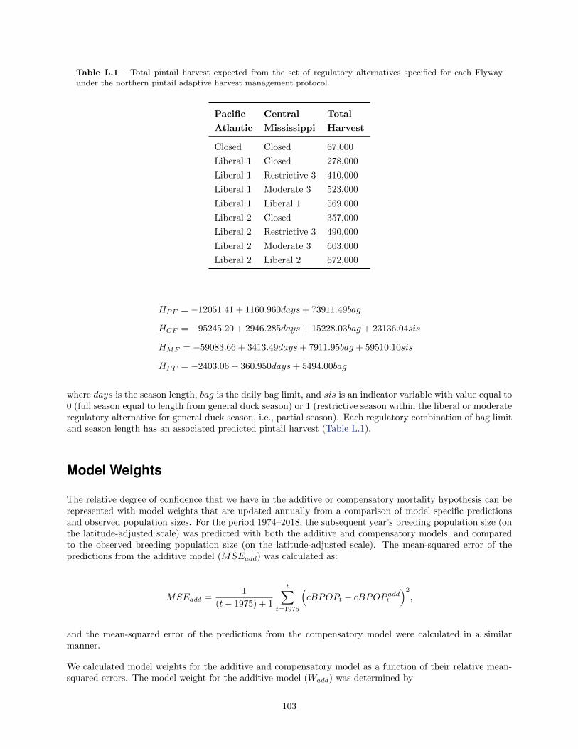
Table L.1 – Total pintail harvest expected from the set of regulatory alternatives specified for each Flywayunder the northern pintail adaptive harvest management protocol.
Pacific Central Total
Atlantic Mississippi Harvest
Closed Closed 67,000
Liberal 1 Closed 278,000
Liberal 1 Restrictive 3 410,000
Liberal 1 Moderate 3 523,000
Liberal 1 Liberal 1 569,000
Liberal 2 Closed 357,000
Liberal 2 Restrictive 3 490,000
Liberal 2 Moderate 3 603,000
Liberal 2 Liberal 2 672,000
𝐻𝑃𝐹 = −12051.41 + 1160.960𝑑𝑎𝑦𝑠+ 73911.49𝑏𝑎𝑔
𝐻𝐶𝐹 = −95245.20 + 2946.285𝑑𝑎𝑦𝑠+ 15228.03𝑏𝑎𝑔 + 23136.04𝑠𝑖𝑠
𝐻𝑀𝐹 = −59083.66 + 3413.49𝑑𝑎𝑦𝑠+ 7911.95𝑏𝑎𝑔 + 59510.10𝑠𝑖𝑠
𝐻𝑃𝐹 = −2403.06 + 360.950𝑑𝑎𝑦𝑠+ 5494.00𝑏𝑎𝑔
where 𝑑𝑎𝑦𝑠 is the season length, 𝑏𝑎𝑔 is the daily bag limit, and 𝑠𝑖𝑠 is an indicator variable with value equal to0 (full season equal to length from general duck season) or 1 (restrictive season within the liberal or moderateregulatory alternative for general duck season, i.e., partial season). Each regulatory combination of bag limitand season length has an associated predicted pintail harvest (Table L.1).
Model Weights
The relative degree of confidence that we have in the additive or compensatory mortality hypothesis can berepresented with model weights that are updated annually from a comparison of model specific predictionsand observed population sizes. For the period 1974–2018, the subsequent year’s breeding population size (onthe latitude-adjusted scale) was predicted with both the additive and compensatory models, and comparedto the observed breeding population size (on the latitude-adjusted scale). The mean-squared error of thepredictions from the additive model (𝑀𝑆𝐸𝑎𝑑𝑑) was calculated as:
𝑀𝑆𝐸𝑎𝑑𝑑 =1
(𝑡− 1975) + 1
𝑡∑𝑡=1975
(𝑐𝐵𝑃𝑂𝑃𝑡 − 𝑐𝐵𝑃𝑂𝑃 𝑎𝑑𝑑
𝑡
)2,
and the mean-squared error of the predictions from the compensatory model were calculated in a similarmanner.
We calculated model weights for the additive and compensatory model as a function of their relative mean-squared errors. The model weight for the additive model (𝑊𝑎𝑑𝑑) was determined by
103
𝑊𝑎𝑑𝑑 =
1
𝑀𝑆𝐸𝑎𝑑𝑑
1
𝑀𝑆𝐸𝑎𝑑𝑑+
1
𝑀𝑆𝐸𝑐𝑜𝑚𝑝
The model weight for the compensatory model was found in a corresponding manner, or by subtracting theadditive model weight from 1.0. As of 2019, the compensatory model did not fit the historic data as wellas the additive model; the model weights were 0.573 for the additive model and 0.427 for the compensatorymodel.
Equilibrium Conditions
Equilibrium analyses of the additive model suggest a carrying capacity of 7.33 million (on the latitude-adjusted scale), maximum sustained yield (MSY) of 446,000 at an equilibrium population size of 3.30 million,and harvest rate of 10.9% (Runge and Boomer 2005). The yield curve resulting from the compensatory modelis significantly skewed compared to the additive model (Figure L.1). Compared to the additive model, thecompensatory model results in a lower carrying capacity (4.67 million), a higher MSY (561 thousand) at alower equilibrium population size (2.99 million), and a higher maximum harvest rate (14.9%).
The average model, based on 2019 model weights, produces a yield curve that is intermediate between theadditive and compensatory models. An equilibrium analysis of the weighted model results in carrying capacity,MSY, equilibrium population size at MSY, and maximum harvest rate that are intermediate between theadditive and compensatory model results (5.45 million, 492 thousand, 3.11 million, and 12.6% respectively).
104

0 2 4 6 8
0.0
0.1
0.2
0.3
0.4
0.5
0.6
0.7
Latitude−adjusted BPOP(in millions)
Ann
ual h
arve
st (
in m
illio
ns)
Additive ModelCompensatory ModelWeighted Model
Figure L.1 – Harvest yield curves resulting from an equilibrium analysis of the northern pintail model set basedon 2019 model weights.
105

Appendix M Scaup Model
We use a state-space formulation of scaup population and harvest dynamics within a Bayesian estimationframework (Meyer and Millar 1999, Millar and Meyer 2000). This analytical framework allows us to repre-sent uncertainty associated with the monitoring programs (observation error) and the ability of our modelformulation to predict actual changes in the system (process error).
Process Model
Given a logistic growth population model that includes harvest (Schaefer 1954), scaup population and harvestdynamics are calculated as a function of the intrinsic rate of increase (r), carrying capacity (K ), and harvest(𝐻𝑡). Following Meyer and Millar (1999), we scaled population sizes by K (i.e., 𝑃𝑡 = 𝑁𝑡/𝐾) and assumed thatprocess errors (𝜖𝑡) are lognormally distributed with a mean of 0 and variance 𝜎2
𝑝𝑟𝑜𝑐𝑒𝑠𝑠. The state dynamicscan be expressed as
𝑃1974 = 𝑃0𝑒𝜀1974
𝑃𝑡 = (𝑃𝑡−1 + 𝑟𝑃𝑡−1 (1− 𝑃𝑡−1)−𝐻𝑡−1/𝐾) 𝑒𝜀𝑡 , 𝑡 = 1975, . . . , 2019,
where 𝑃0 is the initial ratio of population size to carrying capacity. To predict total scaup harvest levels, wemodeled scaup harvest rates (ℎ𝑡) as a function of the pooled direct recovery rate (𝑓𝑡) observed each year with
ℎ𝑡 = 𝑓𝑡/𝜆𝑡.
We specified reporting rate (𝜆𝑡) distributions based on estimates for mallards (Anas platyrhynchos) fromlarge scale historical and existing reward banding studies (Henny and Burnham 1976, Nichols et al. 1995b,P. Garrettson unpublished data). We accounted for increases in reporting rate believed to be associated withchanges in band type (e.g., from AVISE and new address bands to 1-800 toll free bands) by specifying yearspecific reporting rates according to
𝜆𝑡 ∼ 𝑁𝑜𝑟𝑚𝑎𝑙(0.38, 0.04), 𝑡 = 1974, . . . , 1996
𝜆𝑡 ∼ 𝑁𝑜𝑟𝑚𝑎𝑙(0.70, 0.04), 𝑡 = 1997, . . . , 2019.
We then predicted total scaup harvest (𝐻𝑡) with
𝐻𝑡 = ℎ𝑡 [𝑃𝑡 + 𝑟𝑃𝑡 (1− 𝑃𝑡)]𝐾, 𝑡 = 1974, . . . , 2019.
Observation Model
We compared our predictions of population and harvest numbers from our process model to the observationscollected by the Waterfowl and Breeding Habitat Survey (WBPHS) and the Harvest Survey programs withthe following relationships, assuming that the population and harvest observation errors were additive andnormally distributed. May breeding population estimates were related to model predictions by
𝑁𝑂𝑏𝑠𝑒𝑟𝑣𝑒𝑑𝑡 − 𝑃𝑡𝐾 = 𝜀𝐵𝑃𝑂𝑃
𝑡 ,
106

where
𝜀𝐵𝑃𝑂𝑃𝑡 ∼ 𝑁(0, 𝜎2
𝑡,𝐵𝑃𝑂𝑃 ), 𝑡 = 1974, . . . , 2019,
where 𝜎2𝑡,𝐵𝑃𝑂𝑃 is specified each year with the BPOP variance estimates from the WBPHS.
We adjusted our harvest predictions to the observed harvest data estimates with a scaling parameter (q)according to
𝐻𝑂𝑏𝑠𝑒𝑟𝑣𝑒𝑑𝑡 − (ℎ𝑡 [𝑃𝑡 + 𝑟𝑃𝑡 (1− 𝑃𝑡)]𝐾) /𝑞 = 𝜀𝐻𝑡 , 𝑡 = 1974, . . . , 2019,
where,
𝜀𝐻𝑡 ∼ 𝑁(0, 𝜎2𝑡,𝐻𝑎𝑟𝑣𝑒𝑠𝑡).
We assumed that appropriate measures of the harvest observation error 𝜎2𝑡,𝐻𝑎𝑟𝑣𝑒𝑠𝑡 could be approximated by
assuming a coefficient of variation for each annual harvest estimate equal to 0.15 (Paul Padding pers. comm.).The final component of the likelihood included the year specific direct recovery rates that were representedby the rate parameter (𝑓𝑡) of a Binomial distribution indexed by the total number of birds banded preseasonand estimated with,
𝑓𝑡 = 𝑚𝑡/𝑀𝑡,
𝑚𝑡 ∼ 𝐵𝑖𝑛𝑜𝑚𝑖𝑎𝑙(𝑀𝑡, 𝑓𝑡)
where 𝑚𝑡 is the total number of scaup banded preseason in year t and recovered during the hunting seasonin year t and 𝑀𝑡 is the total number of scaup banded preseason in year t.
Bayesian Analysis
Following Meyer and Millar (1999), we developed a fully conditional joint probability model, by first proposingprior distributions for all model parameters and unobserved system states and secondly by developing a fullyconditional likelihood for each sampling distribution.
Prior Distributions
For this analysis, a joint prior distribution is required because the unknown system states P are assumed tobe conditionally independent (Meyer and Millar 1999). This leads to the following joint prior distribution forthe model parameters and unobserved system states
𝑃 (𝑟,𝐾, 𝑞, 𝑓𝑡, 𝜆𝑡, 𝜎2𝑃𝑟𝑜𝑐𝑒𝑠𝑠, 𝑃0, 𝑃1,...,𝑇 ) =
𝑝(𝑟)𝑝(𝐾)𝑝(𝑞)𝑝(𝑓𝑡)𝑝(𝜆𝑡)𝑝(𝜎2𝑃𝑟𝑜𝑐𝑒𝑠𝑠)𝑝(𝑃0)𝑝(𝑃1|𝑃0, 𝜎
2𝑃𝑟𝑜𝑐𝑒𝑠𝑠)
×𝑛∏
𝑡=2
𝑝(𝑃𝑡|𝑃𝑡−1, 𝑟,𝐾, 𝑓𝑡−1, 𝜆𝑡−1, 𝜎2𝑃𝑟𝑜𝑐𝑒𝑠𝑠)
In general, we chose non-informative priors to represent the uncertainty we have in specifying the value ofthe parameters used in our assessment. However, we were required to use existing information to specify
107

informative priors for the initial ratio of population size to carrying capacity (𝑃0) as well as the reportingrate values (𝜆𝑡) specified above that were used to adjust the direct recovery rate estimates to harvest rates.
We specified that the value of 𝑃0, ranged from the population size at maximum sustained yield (𝑃0 =𝑁𝑀𝑆𝑌 /𝐾 = (𝐾/2)/𝐾 = 0.5) to the carrying capacity (𝑃0 = 𝑁/𝐾 = 1), using a uniform distribution on thelog scale to represent this range of values. We assumed that the exploitation experienced at this populationstate was somewhere on the right-hand shoulder of a sustained yield curve (i.e., between MSY and K ). Giventhat we have very little evidence to suggest that historical scaup harvest levels were limiting scaup populationgrowth, this seems like a reasonable prior distribution.
We used non-informative prior distributions to represent the variance and scaling terms, while the priors forthe population parameters r and K were chosen to be vague but within biological bounds. These distributionswere specified according to
𝑃0 ∼ 𝑈𝑛𝑖𝑓𝑜𝑟𝑚(𝑙𝑛(0.5), 0),
𝐾 ∼ 𝐿𝑜𝑔𝑛𝑜𝑟𝑚𝑎𝑙(2.17, 0.667),
𝑟 ∼ 𝑈𝑛𝑖𝑓𝑜𝑟𝑚(0.00001, 2),
𝑓𝑡 ∼ 𝐵𝑒𝑡𝑎(0.5, 0.5),
𝑞 ∼ 𝑈𝑛𝑖𝑓𝑜𝑟𝑚(0.0, 2),
𝜎2𝑃𝑟𝑜𝑐𝑒𝑠𝑠 ∼ 𝐼𝑛𝑣𝑒𝑟𝑠𝑒 𝐺𝑎𝑚𝑚𝑎(0.001, 0.001).
Likelihood
We related the observed population, total harvest estimates, and observed direct recoveries to the modelparameters and unobserved system states with the following likelihood function:
𝑃 (𝑁1,...,𝑇 , 𝐻1,...,𝑇 ,𝑚1,...,𝑇𝑀1,...,𝑇 |𝑟,𝐾, 𝑓𝑡, 𝜆𝑡, 𝑞, 𝜎2𝑃𝑟𝑜𝑐𝑒𝑠𝑠, 𝜎
2𝐻𝑎𝑟𝑣𝑒𝑠𝑡, 𝑃1,...,𝑇 ) =
×𝑇∏
𝑡=1
𝑝(𝑁𝑡|𝑃𝑡,𝐾, 𝜎2𝐵𝑃𝑂𝑃 )×
𝑇∏𝑡=1
𝑝(𝐻𝑡|𝑃𝑡, 𝑟,𝐾, 𝑞, 𝑓𝑡, 𝜆𝑡, 𝜎2𝐻𝑎𝑟𝑣𝑒𝑠𝑡)
×𝑇∏
𝑡=1
𝑝(𝑚𝑡|𝑀𝑡, 𝑓𝑡)
Posterior Evaluation
Using Bayes theorem we then specified a posterior distribution for the fully conditional joint probabilitydistribution of the parameters given the observed information according to
𝑃 (𝑟,𝐾, 𝑞, 𝑓𝑡, 𝜆𝑡, 𝜎2𝑃𝑟𝑜𝑐𝑒𝑠𝑠, 𝑃0, 𝑃1,...,𝑇 |𝑁1,...,𝑇 , 𝐻1,...,𝑇 ,𝑚1,...,𝑇 ,𝑀1,...,𝑇 ) ∝
𝑝(𝑟)𝑝(𝐾)𝑝(𝑞)𝑝(𝑓𝑡)𝑝(𝜆𝑡)𝑝(𝜎2𝑃𝑟𝑜𝑐𝑒𝑠𝑠)𝑝(𝑃0)𝑝(𝑃1|𝑃0, 𝜎
2𝑃𝑟𝑜𝑐𝑒𝑠𝑠)
×𝑛∏
𝑡=2
𝑝(𝑃𝑡|𝑃𝑡−1, 𝑟,𝐾, 𝑓𝑡−1, 𝜆𝑡−1, 𝜎2𝑃𝑟𝑜𝑐𝑒𝑠𝑠)×
𝑇∏𝑡=1
𝑝(𝑁𝑡|𝑃𝑡,𝐾, 𝜎2𝐵𝑃𝑂𝑃 )
×𝑇∏
𝑡=1
𝑝(𝐻𝑡|𝑃𝑡, 𝑟,𝐾, 𝑞, 𝑓𝑡, 𝜆𝑡, 𝜎2𝐻𝑎𝑟𝑣𝑒𝑠𝑡)×
𝑇∏𝑡=1
𝑝(𝑚𝑡|𝑀𝑡, 𝑓𝑡)
108

Table M.1 – Model parameter estimates resulting from a Bayesian analysis of scaup breeding population,harvest, and banding information from 1974 to 2019.
Parameter Mean SD 2.5% CI Median 97.5% CI
r 0.1342 0.0451 0.0634 0.1277 0.2409
K 8.7645 1.6932 6.2250 8.5055 12.5000
𝜎2 0.0078 0.0031 0.0034 0.0072 0.0151
q 0.7550 0.0402 0.6806 0.7536 0.8397
We used MCMC methods to evaluate the posterior distribution using WinBUGS (Spiegelhalter et al. 2003).We randomly generated initial values and simulated 5 independent chains each with 1,000,000 iterations. Wediscarded the first half of the simulation and thinned each chain by 250, yielding a sample of 10,000 points.We calculated Gelman-Rubin statistics (Brooks and Gelman 1998) to monitor for lack of convergence. Thestate-space formulation and Bayesian analysis framework provided reasonable fits to the observed breedingpopulation and total harvest estimates with realistic measures of variation. The 2019 posterior estimates ofmodel parameters based on data from 1974 to 2019 are provided in Table M.1.
We further summarized the simulation results for r, K, and the scaling parameter q to admit parametricuncertainty with a formal correlation structure within the optimization procedure used to calculate theharvest strategy. We first defined a joint distribution for 3 discrete outcomes for each of the 3 populationparameters. We used the 30 and 70 percent quantiles for each parameter as the cut points to define threebins for which to discretize 3 values of each posterior distribution. We then determined the frequency ofoccurrence of each of the 27 possible combinations of each parameter value falling within the 3 bins from theMCMC simulation results. These frequencies were then assigned parameter values based on the midpoint ofthe bin ranges (15, 50, 85 percent quantiles) to specify the joint distribution of the population parametervalues used in the optimization.
109