user's manual mexico landfill gas model - globalmethane.org · recovery recorded at the...
TRANSCRIPT

March 2009
Users Manual Mexico Landfill Gas Model
Version 20
Prepared on behalf of
Victoria Ludwig Landfill Methane Outreach Program
US Environmental Protection Agency Washington DC
Prepared by
G Alex Stege Jose Luis Davila SCS Engineers
Phoenix AZ 85008 EPA Contract EP-W-06-023
Task Order 30
Project Manager Dana L Murray PE
SCS Engineers Reston VA 20190
DISCLAIMER
This userrsquos guide has been prepared specifically for Mexico on behalf of the Landfill Methane
Outreach Program US Environmental Protection Agency as part of the Methane to
Markets program activities in Mexico The methods contained within are based on
engineering judgment and represent the standard of care that would be exercised by a
professional experienced in the field of landfill gas projections The US EPA and SCS
Engineers do not guarantee the quantity of available landfill gas and no other warranty is
expressed or implied No other party is intended as a beneficiary of this work product its
content or information embedded therein Third parties use this guide at their own risk
The US EPA and SCS Engineers assume no responsibility for the accuracy of information
obtained from compiled or provided by other parties
i
ABSTRACT
This document is a users guide for a computer model Mexico Landfill Gas Model Version
20 (Model) for estimating landfill gas (LFG) generation and recovery from municipal solid
waste landfills in Mexico The Model was developed by SCS Engineers under contract to the
US EPArsquos Landfill Methane Outreach Program (LMOP) The Model can be used to estimate
landfill gas generation rates from landfills and potential landfill gas recovery rates for
landfills that have or plan to have gas collection and control systems in Mexico
The Model is an Excelreg spreadsheet model that calculates LFG generation by applying a first
order decay equation The model requires the user to input site-specific data for landfill
opening and closing years refuse disposal rates landfill location and to answer several
questions regarding the past and current physical conditions of the landfill The model
provides default values for waste composition and input variables (k and L0) for each state
and estimates the collection efficiency based on the answers provided The default values
were developed using data on climate waste characteristics and disposal practices in
Mexico and the estimated effect of these conditions on the amounts and rates of LFG
generation Actual LFG recovery rates from four landfills in Mexico were evaluated to help
guide the selection of model k and L0 values
The Model was developed with the goal of providing accurate and conservative projections
of LFG generation and recovery Other models evaluated during the model development
process included the Mexico LFG Model Version 10 and the Intergovernmental Panel on
Climate Change (IPCC) 2006 Waste Model (IPCC Model) The Model incorporated waste
composition data used to develop the Mexico LFG Model Version 10 and expanded the data
to include information from additional cities and landfills throughout Mexico The Model also
incorporated the structure of the IPCC Model with revised input assumptions to make it
better reflect local climate and conditions at disposal sites in Mexico
ii
TABLE OF CONTENTS
Section Page
DISCLAIMER i ABSTRACT ii TABLE OF CONTENTS iii LIST OF FIGURESiii LIST OF TABLES iii GLOSSARY OF TERMSiv 10 Introduction 1 20 Model Description 5
21 Background on the Old (Version 10) Mexico LFG Model 5 22 Mexico LFG Model Version 20 6
221 Model k Values 6 222 Waste Composition and Potential Methane Generation Capacity (L0) 7 223 Methane Correction Factor 8 224 Adjustments for Fire Impacts 9 225 Estimating Collection Efficiency and LFG Recovery 9
30 Model Instructions 16 31 Inputs Worksheet 17 32 Disposal amp LFG Recovery Worksheet 17
321 Waste Disposal Estimates 17 322 Actual LFG Recovery 21 323 Collection Efficiency 21 324 Baseline LFG Recovery 21
33 Waste Composition 22 34 Model Outputs - Table 23 35 Model Outputs - Graph 25
40 References 27
LIST OF FIGURES
Figure Page
1 Mexico Climate Regions 3 2 Inputs Section Inputs Worksheet 18 3 Instructions Section Inputs Worksheet 19 4 Inputs Section Disposal amp LFG Recovery Worksheet 20 5 Instructions Section Disposal amp LFG Recovery Worksheet 22 6 Portion of Waste Composition Worksheet 23 7 Sample Model Output Table 24 8 Sample Model Output Graph 26
LIST OF TABLES
Table Page
1 Methane Generation Rate (k) Values by Waste Category and Region 7 2 Potential Methane Generation Capacity (L0) Values 8 3 Methane Correction Factor (MCF) 9
iii
GLOSSARY OF TERMS
Actual Landfill Gas (LFG) Recovery (m3hr at 50 CH4) - Annual average LFG recovery recorded at the blowerflare station in cubic meters per hour normalized at 50 methane For instructions on how to normalize to 50 see Section 22 of the manual
Baseline Landfill Gas (LFG) Recovery (m3hr at 50 CH4) - This term is applicable for projects looking to pursue carbon credits and is defined as the amount of LFG recovery that was occurring prior to the start up of the LFG project and would continue to occur (as required by applicable regulations or common practices) For a precise definition of baseline recovery and emissions for Clean Development Mechanism (CDM) projects please refer to the ldquoGlossary of CDM Termsrdquo available on the UNFCCC website at httpcdmunfcccintReferenceGuidclarifglos_CDM_v04pdf
Closure Year - The year in which the landfill ceases or is expected to cease accepting waste
Collection System Efficiency - The estimated percentage of generated landfill gas which is or can be collected in a gas collection system Collection efficiency is a function of both collection system coverage and the efficiency of collection system operations
Collection System Coverage - The estimated percentage of a landfillrsquos refuse mass that is potentially within the influence of a gas collection systemrsquos extraction wells
Design Capacity of the Landfill - The total amount of refuse that can be disposed of in the landfill calculated in terms of volume (m3) or mass (Mg)
Garden Waste ndash The fraction of the total waste stream that contains plants trimmings from homes or city parks (also known as green waste)
Landfill Gas - Landfill gas is a product of biodegradation of refuse in landfills and consists of primarily methane and carbon dioxide with trace amounts of non-methane organic compounds and air pollutants
Landfill Gas (LFG) Generation - Total amount of LFG produced by the decomposition of the organic waste present at a landfill
Landfill Gas (LFG) Recovery - The fraction of the LFG generation that is or can be captured by a landfill gas collection and control system Modeled LFG recovery is calculated by multiplying the LFG generation rate by the collection system efficiency
Managed Landfill - A managed landfill is defined as having controlled placement of waste (waste directed to specific disposal areas a degree of control of scavenging and fires) and one or more of the following cover material mechanical compacting or leveling of waste
Methane Correction Factor (MCF)- Adjustment to model estimates of LFG generation that accounts for the degree to which waste decays anaerobically (See section 1221 for more details)
iv
Methane Generation Rate Constant (k)- Model constant that determines the estimated rate at which waste decays and generates LFG The k value is related to the
ln(2)half-life of waste (t12) according to the formula t1 2 = The k is a function of the
k moisture content in the landfill refuse availability of nutrients for methanogens pH and temperature (Units = 1year)
Potential Methane Generation Capacity (Lo)- Model constant that represents the maximum amount of methane (a primary constituent of LFG) which can be generated from a fixed amount of waste given an infinite period of time for it to decompose Lo depends on the amount of cellulose in the refuse (Units = m3Mg)
Semi-Aerobic Landfill - A semi-aerobic landfill has controlled placement of waste and all of the following structures for introducing air into the waste layer permeable cover material leachate drainage system and gas ventilation system
Unmanaged Waste Disposal Site ndash An unmanaged waste disposal site is a dump site that does not meet the definition of a managed waste disposal site
Waste Disposal Estimates (Metric Tonnes or Mg)- Annual total waste disposal tonnages recorded at the scale-house or estimated using other methods
v
1 0 INTRODUCTION
Landfill gas (LFG) is generated by the decomposition of refuse in a landfill under anaerobic
conditions and can be recovered through the operation of gas collection and control
systems that typically burns the gas in flares Alternatively the collected gas can be used
beneficially Beneficial uses of LFG include use as fuel in energy recovery facilities such as
internal combustion engines gas turbines microturbines steam boilers or other facilities
that use the gas for electricity or heat generation
In addition to the energy benefits from the beneficial use of LFG collection and control of
generated LFG helps to reduce LFG emissions that are harmful to the environment The US
EPA has determined that LFG emissions from municipal solid waste (MSW) landfills cause or
contribute significantly to air pollution that may reasonably be anticipated to endanger
public health or welfare Some are known or suspected carcinogens or cause other nonshy
cancerous health effects Public welfare concerns include the odor nuisance from the LFG
and the potential for methane migration both on-site and off-site which may lead to
explosions or fires The methane emitted from landfills is also a concern because it is a
greenhouse gas thereby contributing to the challenge of global climate change
The main purpose of the Mexico LFG Model (Model) is to provide landfill owners and
operators in Mexico with a tool to use to evaluate the feasibility and potential benefits of
collecting and using the generated LFG for energy recovery or other uses To fulfill this
purpose the Model uses Excelreg spreadsheet software to calculate LFG generation by
applying a first order decay equation The Model provides LFG recovery estimates by
multiplying the calculated amount of LFG generation by estimates of the efficiency of the
collection system in capturing generated gas which is known as the collection efficiency
The Model uses the following information to estimate LFG generation and recovery from a
landfill (see the Glossary of Terms)
bull The amounts of waste disposed at the landfill annually
bull The opening and closing years of landfill operation
bull The methane generation rate (k) constant
bull The potential methane generation capacity (L0)
bull The methane correction factor (MCF)
bull The fire adjustment factor (F)
Mexico LFG Model Version 20 Userrsquos Manual 1 32009
bull The collection efficiency of the gas collection system
The model estimates the LFG generation rate in a given year using the following first-order
exponential equation which was modified from the US EPArsquos Landfill Gas Emissions Model
(LandGEM) version 302 (EPA 2005)
n 1 MiQLFG = sumsum2kL0[ ] (e-ktij) (MCF) (F)
t =1 j=01 10
Where QLFG = maximum expected LFG generation flow rate (m3yr) i = 1 year time increment n = (year of the calculation) ndash (initial year of waste acceptance) j = 01 year time increment k = methane generation rate (1yr) Lo = potential methane generation capacity (m3Mg) Mi = mass of solid waste disposed in the ith year (Mg) tij = age of the jth section of waste mass Mi disposed in the ith year (decimal
years) MCF = methane correction factor F = fire adjustment factor
The above equation is used to estimate LFG generation for a given year from cumulative
waste disposed up through that year Multi-year projections are developed by varying the
projection year and then re-applying the equation Total LFG generation is equal to two
times the calculated methane generation1 The exponential decay function assumes that
LFG generation is at its peak following a time lag representing the period prior to methane
generation The model assumes a six month time lag between placement of waste and LFG
generation For each unit of waste after six months the model assumes that LFG generation
decreases exponentially as the organic fraction of waste is consumed The year of maximum
LFG generation normally occurs in the closure year or the year following closure (depending
on the disposal rate in the final years)
The Model estimates of LFG generation and recovery in cubic meters per hour (m3hr) and
cubic feet per minute (cfm) It also estimates the energy content of generated and
recovered LFG in million British Thermal Units per hour (mmBtuhr) the system collection
efficiency the maximum power plant capacity that could be fueled by the collected LFG
(MW) and the emission reductions in tonnes of CO2 equivalent (CERs) achieved by the
collection and combustion of the LFG
1 The composition of landfill gas is assumed by the Model to consist of 50 percent methane (CH4) and 50 percent other gases including carbon dioxide (CO2) and trace amounts of other compounds
Mexico LFG Model Version 20 Userrsquos Manual 2 32009
The Model can either calculate annual waste disposal rates and collection efficiency
automatically using the information provided by the user in the ldquoInputsrdquo worksheet or the
user can manually input annual waste disposal rates and collection efficiency estimates in
the ldquoDisposal amp LFG Recoveryrdquo worksheet The model automatically assigns values for k
and L0 based on climate and waste composition data The k values vary depending on
climate and waste group The L0 values vary depending on waste group Climate is
categorized into one of five climate regions within Mexico based on average annual
precipitation and temperature (see Figure 1) Each state is assigned to a climate region
Waste categories are assigned to one of five groups including four organic waste groups
based on waste decay rates and one inorganic waste group If site-specific waste
composition data are available the user can enter the waste composition data in the ldquoWaste
Compositionrdquo worksheet Otherwise the model will assign the default waste composition
percentages for the selected state which are based on waste composition data gathered
from the state or from other states within the same climate region
Figure 1 Mexico Climate Regions
Mexico LFG Model Version 20 Userrsquos Manual 3 32009
The annual waste disposal rates k and L0 values methane correction and fire adjustment
factors and collection efficiency estimates are used to produce LFG generation and recovery
estimates for landfills located in each state in Mexico Model results are displayed in the
ldquoOutput-Tablerdquo and ldquoOutput-Graphrdquo worksheets
EPA recognizes that modeling LFG generation and recovery accurately is difficult due to
limitations in available information for inputs to the model However as new landfills are
constructed and operated and better information is collected the present modeling
approach can be improved In addition as more landfills in Mexico develop gas collection
and control systems additional data on LFG generation and recovery will become available
for model calibration and the development of improved model default values
Questions and comments concerning the LFG model should be directed to Victoria Ludwig of
EPAs LMOP at LudwigVictoriaepamailepagov
Mexico LFG Model Version 20 Userrsquos Manual 4 32009
2 0 MODEL DESCRIPTION
2 1 B a c k g r o u n d o n t h e O l d ( V e r s i o n 1 0 ) M e x i c o L F G M o d e l
The first version of the Mexico Landfill Gas Model (v 10) which was presented in
December 2003 was developed by SCS Engineers for the SEDESOL IIE and CONAE under
a contract with LMOP and USAID This model applied single k and L0 values to the LandGEM
equation which were assigned based on average annual precipitation at the landfill location
The k values were estimated based on models prepared for two landfills in Mexico and
general observations at US landfills regarding the variation in k with precipitation The L0
values were assigned based on the average composition of wastes in Mexico derived from
data from 31 cities
In 2008 LMOP contracted with SCS Engineers to develop an updated and improved version
of the Mexico LFG Model Some of the shortcomings of the original model which were
targeted for revision included the following
bull The model assumed an average waste composition for all of Mexico and did not
account for region or state-specific variations or allow for the user to input site-
specific waste composition values if available Variations in waste composition can
have a large impact on LFG generation For example Mexico City has a significantly
lower organic content in the waste stream
bull The application of a single k value in the LandGEM equation assumes a single decay
rate for all wastes in a landfill and does not account for variations in the average
decay rates over time This becomes a significant source of error when a large
percentage of wastes consists of food and other rapidly decaying materials In
Mexico and other developing countries with a large food waste component single k
models tend to over-estimate LFG generation in wet climates after the landfill closes
and under-estimate LFG generation in dry climates while the landfill is still receiving
wastes
bull The default k values were based on a limited amount of data from only two landfills
(Simeprodeso Landfill in Monterrey was the only site with complete flow data)
bull The model used an outdated version of the LandGEM equation
bull The model did not include estimates of certified emission reductions (CERs)
bull The model required the user to input detailed waste disposal rates and to evaluate
collection efficiency
Mexico LFG Model Version 20 Userrsquos Manual 5 32009
2 2 M e x i c o L F G M o d e l V e r s i o n 2 0
The Mexico LFG Model Version 20 (March 2009) provides an automated estimation tool for
quantifying LFG generation and recovery from MSW landfills in all states of Mexico The
Model applies separate equations to calculate LFG generation from each of the following four
organic waste2 categories that are grouped according to waste decay rates
1 Very fast decaying waste ndash food waste other organics 20 of diapers
2 Medium fast decaying waste ndash garden waste (green waste) toilet paper
3 Medium slow decaying waste ndash paper and cardboard textiles
4 Slowly decaying waste ndash wood rubber leather bones straw
Total LFG generation for all wastes is calculated as the sum of the amounts of LFG
generated by each of the four organic waste categories Each of the four organic waste
groups are assigned different k and L0 pairs that are used to calculate LFG generation The
Modelrsquos calculations of LFG generation also include an adjustment to account for aerobic
waste decay known as the methane correction factor (MCF) and an adjustment to account
for the extent to which the site has been impacted by fires LFG recovery is estimated by
the Model by multiplying projected LFG generation by the estimated collection efficiency
Each of these variables ndash k L0 MCF fire impact adjustments and collection efficiency ndash are
discussed in detail below
2 2 1 M o d e l k V a l u e s
The methane generation rate constant k determines the rate of generation of methane
from refuse in the landfill The units for k are in year-1 The k value describes the rate at
which refuse placed in a landfill decays and produces methane and is related to the half-life
of waste according to the equation half-life = ln(2)k The higher the value of k the faster
total methane generation at a landfill increases (as long as the landfill is still receiving
waste) and then declines (after the landfill closes) over time
The value of k is a function of the following factors (1) refuse moisture content (2)
availability of nutrients for methane-generating bacteria (3) pH and (4) temperature
Moisture conditions inside a landfill typically are not well known and are estimated based on
average annual precipitation Availability of nutrients is a function of waste amounts and
waste composition The pH inside a landfill is generally unknown and is not evaluated in the
model Temperature in a landfill is relatively constant due to the heat generated by
Mexico LFG Model Version 20 Userrsquos Manual 6 32009
anaerobic bacteria and tends to be independent of outside temperature except in shallow
landfills in very cold climates Therefore the Model estimates k values based on waste type
and climate
The four waste categories listed above have been assigned different k values to reflect
differences in waste decay rates The k values assigned to each of the four waste groups
also vary based on the average annual precipitation in the climate region where the landfill
is located Each state is assigned to one of the 5 climate regions shown in Figure 1 based
on average annual precipitation3 The k values that the Model uses for each waste category
and region are shown in Table 1
Table 1 Methane Generation Rate (k) Values by Waste Category and Region
Waste Category
Region 1 Region 2 Region 3 Region 4 Region 5
Southeas t
West Central Interior
Northeas t
Northeast amp Interior North
1 0300 0220 0160 0150 0100 2 0130 0100 0075 0070 0050 3 0050 0040 0032 0030 0020 4 0025 0020 0016 0015 0010
Includes Federal District
2 2 2 W a s t e C o m p o s i t i o n a n d P o t e n t i a l M e t h a n e G e n e r a t i o n C a p a c i t y ( L 0 )
The value for the potential methane generation capacity of refuse (L0) describes the total
amount of methane gas potentially produced by a tonne of refuse as it decays and depends
almost exclusively on the composition of wastes in the landfill A higher cellulose content in
refuse results in a higher value of L0 The units of L0 are in cubic meters per tonne of refuse
(m3Mg) The values of theoretical and obtainable L0 range from 62 to 270 m3Mg refuse
(EPA 1991)
The L0 values used in the Model are derived from waste composition data from 40 cities
(including 3 landfills in Mexico City) that represent 18 states and the Federal District
Average waste composition was calculated for each state and each region using population
2 Inorganic waste does not generate LFG and is excluded from the model calculations 3 A statersquos average annual precipitation was estimated using data from wwwworldclimatecom wwwweatherbasecom or wwwworldweatherorg from the statersquos largest cities Statersquos averages were calculated from the data using population as a weighting factor
Mexico LFG Model Version 20 Userrsquos Manual 7 32009
to weight the contribution of each data set to the average States that had no waste
composition data available were assigned the regional average waste composition Default
waste composition values for each state are used by the Model unless the user indicates
that they have site-specific waste composition data in the ldquoInputsrdquo worksheet and enters
the data in the ldquoWaste Compositionrdquo worksheet
The model uses the state default or site-specific waste composition data to calculate L0
values for each of the four waste categories The L0 values which are used by the Model are
shown in Table 2 The L0 values for each waste group are assumed to remain constant
across all climates except for Category 2 which will have some variation with climate due
to differences in the types of vegetation included in the green waste
Table 2 Potential Methane Generation Capacity (L0) Values
Waste Category
Region 1 Region 2 Region 3 Region 4 Region 5
Southeas t
West Central Interior
Northeas t
Northeast amp Interior North
1 69 69 69 69 69 2 115 126 138 138 149 3 214 214 214 214 214 4 202 202 202 202 202
Includes Federal District
2 2 3 M e t h a n e C o r r e c t i o n F a c t o r
The Methane Correction Factor (MCF) is an adjustment to model estimates of LFG
generation that accounts for the degree to which wastes decay aerobically The MCF varies
depending on waste depth and landfill type as defined by site management practices At
managed sanitary landfills all waste decay is assumed to be anaerobic (MCF of 1) At
landfills or dumps with conditions less conducive to anaerobic decay the MCF will be lower
to reflect the extent of aerobic conditions at these sites Table 3 summarizes the MCF
adjustments applied by the model based on information on waste depths and site
management practices that are provided by the user in response to Questions 11 and 12
in the ldquoInputsrdquo worksheet
Mexico LFG Model Version 20 Userrsquos Manual 8 32009
Table 3 Methane Correction Factor (MCF)
Site Management Depth lt5m Depth gt=5m
Unmanaged Disposal Site 04 08 Managed Landfill 08 10
Semi-Aerobic Landfill 04 05 Unknown 04 08
Waste depth of at least five meters promotes anaerobic decay at shallower sites waste
decay may be primarily aerobic A managed landfill is defined as having controlled
placement of waste (waste directed to specific disposal areas a degree of control of
scavenging and fires) and one or more of the following cover material mechanical
compacting or leveling of waste (IPCC 2006) A semi-aerobic landfill has controlled
placement of waste and all of the following structures for introducing air into the waste
layer permeable cover material leachate drainage system and gas ventilation system
(IPCC 2006)
2 2 4 A d j u s t m e n t s f o r F i r e I m p a c t s
Landfill fires consume waste as a fuel and leave behind ash that does not produce LFG LFG
generation can be significantly impacted at landfills that have had a history of fires Model
users are asked if the site has been impacted by fires in Question 13a in the ldquoInputsrdquo
worksheet If the answer is yes the user is asked to answer questions on the percent of
landfill area impacted by fires and the severity of fire impacts The Model discounts LFG
generation by the percent of landfill area impacted multiplied by an adjustment for severity
of impacts (13 for low impacts 23 for medium impacts and 1 for severe impacts)
2 2 5 E s t i m a t i n g C o l l e c t i o n E f f i c i e n c y a n d L F G R e c o v e r y
Collection efficiency is a measure of the ability of the gas collection system to capture
generated LFG It is a function of both system design (how much of the landfill does the
system collect from) and system operations and maintenance (is the system operated
efficiently and well-maintained) Collection efficiency is a percentage value that is applied
to the LFG generation projection produced by the model to estimate the amount of LFG that
is or can be recovered for flaring or beneficial use Although rates of LFG recovery can be
measured rates of generation in a landfill cannot be measured (hence the need for a model
Mexico LFG Model Version 20 Userrsquos Manual 9 32009
to estimate generation) therefore considerable uncertainty exists regarding actual
collection efficiencies achieved at landfills
In response to the uncertainty regarding collection efficiencies the US EPA (EPA 1998)
published what it believed are reasonable collection efficiencies for landfills in the US that
meet US design standards and have ldquocomprehensiverdquo gas collection systems According to
the EPA collection efficiencies at such landfills typically range from 60 to 85 with an
average of 75 More recently a report by the Intergovernmental Panel on Climate Change
(IPCC 2006) stated that ldquogt90 recovery can be achieved at cells with final cover and an
efficient gas extraction systemrdquo While modern sanitary landfills in Mexico can achieve
maximum collection efficiencies of greater than 90 under the best conditions unmanaged
disposal sites may never exceed 50 collection efficiency even with a comprehensive
system
The Model calculates collection efficiency automatically based on user responses to a series
of questions in the ldquoInputsrdquo worksheet The calculation method that the model uses is
described below in Subsection 2251 Alternatively the user can override the Modelrsquos
calculations and manually input estimated collection efficiencies We recommend that the
user keep the automatic collection efficiency calculations intact unless the site already has a
gas collection system in place and flow data is available The process for manually
adjusting collection efficiency so that the LFG recovery rates projected by the Model match
actual recovery are described in Subsection 2252
2251 Model Calculation of Collection Efficiency
The Model automatically calculates collection efficiency based on the following factors
bull Collection system coverage ndash collection efficiency is directly related to the extent of
wellfield coverage of the refuse mass
bull Waste depth ndash shallow landfills require shallow wells which are less efficient because
they are more prone to air infiltration
bull Cover type and extent ndash collection efficiencies will be highest at landfills with a low
permeable soil cover over all areas with waste which limits the release of LFG into
the atmosphere air infiltration into the gas system and rainfall infiltration into the
waste
bull Landfill liner ndash landfills with clay or synthetic liners will have lower rates of LFG
migration into surrounding soils resulting in higher collection efficiencies
Mexico LFG Model Version 20 Userrsquos Manual 10 32009
bull Waste compaction ndash uncompacted waste will have higher air infiltration and lower
gas quality and thus lower collection efficiency
bull Size of the active disposal (ldquotippingrdquo) area ndash unmanaged disposal sites with large
tipping areas will tend to have lower collection efficiencies than managed sites where
disposal is directed to specific tipping areas
bull Leachate management ndash high leachate levels can dramatically limit collection
efficiencies particularly at landfills with high rainfall poor drainage and limited soil
cover
Each of these factors are discussed below While answering the questions in the Inputs
worksheet which are described below the model user should understand that conditions
which affect collection efficiency can change over time as landfill conditions change For
example the landfill depth or the estimated percentages of area with each cover type (final
intermediate and daily) often will change over time We recommend that the model userrsquos
answers to the questions reflect current conditions if a gas collection system is already
installed If no system is installed the model user should try to estimate the future
conditions that will occur in the year that the system will begin operation The calculated
collection efficiency will then reflect conditions in the current year or the first year of system
operation Adjustments to later yearsrsquo collection efficiency estimates can be guided by
actual recovery data using a process that is described in Subsection 2252
Collection System Coverage
Collection system coverage describes the percentage of the waste that is within the
influence of the existing or planned extraction wells It accounts for system design and the
efficiency of wellfield operations Most landfills particularly those that are still receiving
wastes will have considerably less than 100 percent collection system coverage Sites with
security issues or large numbers of uncontrolled waste pickers will not be able to install
equipment in unsecured areas and cannot achieve good collection system coverage
The Model user is requested to estimate current or future collection system coverage in
Question 15 of the ldquoInputsrdquo worksheet which asks for ldquoPercent of waste area with wellsrdquo
Estimates of collection system coverage at landfills with systems already in operation should
include discounts for non-functioning wells The importance of a non-functioning well
should be taken into account when estimating the discount for non-functioning wells For
example a site with a non-functioning well in the vicinity of other wells that are functional
Mexico LFG Model Version 20 Userrsquos Manual 11 32009
should cause less of a collection efficiency discount than a site with a non-functioning well
that is the only well in the area available to draw LFG from a significant portion of the site
Evaluation of collection system coverage requires a fair degree of familiarity with the system
design Well spacing and depth are important factors The following describes the various
scenarios to consider
bull Deeper wells can draw LFG from a larger volume of refuse than shallow wells
because greater vacuum can be applied to the wells without drawing in air from the
surface
bull Landfills with deep wells (greater than about 20 meters) can effectively collect LFG
from all areas of the site with vertical well densities as low as two wells or less per
hectare
bull Landfills with shallower wells will require greater well densities perhaps more than 2
wells per hectare to achieve the same coverage
Although landfills with a dense network of wells will collect more total gas than landfills with
more widely spaced wells landfills with a small number of well-spaced wells typically collect
more gas per well (due to their ability to influence a larger volume of refuse per well) than
wells at landfills with a dense network of wells
Waste Depth
Deeper waste depths allow deeper wells to be installed As noted in the above discussion of
collection system coverage deeper wells can operate more effectively than shallow wells
because a greater vacuum can be applied to the wells Wells installed in shallow waste less
than about 10m will tend to have greater air infiltration Model users are requested to input
average landfill depth in Question 11 in the ldquoInputsrdquo worksheet The Model assumes a 5
discount to estimated collection efficiency for every 1m of waste depth less than 10m
Cover Type and Extent
The type and extent of landfill cover can have a significant influence on achievable collection
efficiency Unmanaged disposal sites with little or no soil cover will have high rates of LFG
emissions into the atmosphere and air infiltration into the collection system resulting in
lower rates of LFG capture Areas without a soil cover also will have high rates of rainfall
infiltration causing leachate levels to build up and cause the gas collection system to be
blocked with liquids Installation of a soil cover will decrease LFG emissions and lower air
and rainfall infiltration These effects will depend on cover permeability cover thickness
Mexico LFG Model Version 20 Userrsquos Manual 12 32009
and the percentage of landfill area with cover Typically a final cover will have the greatest
thickness and lowest permeability and will be the most effective in terms of increasing
collection efficiency Most landfills will have at least an intermediate soil cover installed over
areas that have not been used for disposal for an extended period intermediate soils
provide a moderate level of control over air infiltration LFG emissions and rainfall
infiltration Daily soil cover typically is a shallower layer of soil that is installed at the end of
the day in active disposal areas and provides a more permeable barrier to air and water
than final or intermediate cover soils
Model users are asked to estimate the percentage of landfill area with each soil cover type
in Questions 16 17 and 18 in the ldquoInputsrdquo worksheet The Model automatically calculates
the percentage of landfill area with no soil cover as the remaining area The Model
calculates a weighted average collection efficiency adjustment to account for the
percentages of each soil cover type by assigning 90 collection efficiency to the percentage
of landfill area with final cover 80 collection efficiency to the percentage of landfill area
with intermediate cover 75 collection efficiency to the percentage of landfill area with
daily soil cover and 50 collection efficiency to the percentage of landfill area with no soil
cover
Landfill Liner
Clay or synthetic bottom liners act as a low-permeability barrier which is effective at limiting
off-site LFG migration into surrounding soils particularly when there is an active LFG
collection system operating Model users are asked to estimate the percentage of landfill
area with a clay or synthetic bottom liner in Question 20 in the ldquoInputsrdquo worksheet The
Model calculates a discount to collection efficiency equal to 5 times the percent area
without a clay or synthetic liner
Waste Compaction
Waste compaction helps promote anaerobic waste decay and tends to improve collection
efficiency by limiting air infiltration and improving gas quality Model users are asked if
waste compaction occurs on a regular basis in Question 21 of the ldquoInputsrdquo worksheet
Collection efficiency is discounted by 3 if regular waste compaction does not occur
Focused Tipping Area
Mexico LFG Model Version 20 Userrsquos Manual 13 32009
Landfills where waste delivery trucks are directed to unload wastes in a specific area will
provide better management of disposed wastes including more efficient compaction more
frequent and extensive soil covering of exposed wastes and higher waste depths all of
which contribute to higher collection efficiencies Model users are asked if waste is
delivered to a focused tipping area in Question 22 of the ldquoInputsrdquo worksheet Collection
efficiency is discounted by 5 if waste is not delivered to a focused tipping area
Leachate
Leachate almost always limits effective collection system operations at landfills in
developing countries due to the high waste moisture content and the lack of proper
drainage Areas with heavy rainfall are especially susceptible to leachate buildup in the
landfill High leachate levels in a landfill can dramatically limit collection efficiency by
blocking well perforations and preventing wells from applying vacuum to draw in LFG from
the surrounding waste mass Unless the climate is extremely dry or the landfill has been
designed to provide good management of liquids through proper surface drainage and cost
effective systems for collection and treatment of leachate the landfill often will show signs
of the accumulation of liquids through surface seeps or ponding This evidence of high
leachate levels in the landfill may be temporary features that appear only after rainstorms
suggesting that leachate problems may be less severe or they may persist for longer
periods suggesting that high leachate levels are an ongoing problem
The impacts of leachate on collection efficiency are evaluated by the Model based on
evidence of leachate at the landfill surface whether the evidence appears only after
rainstorms and climate Model users are asked if the landfill experiences leachate surface
seeps or surface ponding in Question 23a of the ldquoInputsrdquo worksheet If the answer is yes
the Model user is asked in Question 23b if this occurs only after rainstorms If evidence of
leachate accumulation appears only after rainstorms the Model applies a 2 to 15
discount to collection efficiency depending on climate (rainy climates receive a higher
discount) If the evidence of leachate accumulation persists between rainstorms the Model
applies a 10 to 40 discount to collection efficiency depending on climate
Model Estimate of Collection Efficiency
The Model calculates collection efficiency as the product of all the factors listed above If
the collection efficiency factor involves a discount a value of one minus the discount is used
in the calculation Each step in the collection efficiency calculation and the resulting
Mexico LFG Model Version 20 Userrsquos Manual 14 32009
collection efficiency estimate are shown in Cells J15 through J22 of the ldquoDisposal amp LFG
Recoveryrdquo worksheet The calculated collection efficiency value also is displayed in Column
D of the ldquoDisposal amp LFG Recoveryrdquo worksheet for each year starting with the year of initial
collection system start up indicated by the Model user in response to Question 14 in the
ldquoInputsrdquo worksheet
2252 Adjustments to Collection Efficiency
Accurate estimates of collection efficiency can be difficult to achieve given all of the
influencing factors described above The accuracy of the estimate tends to be higher when
collection efficiency is high and lower when collection efficiency is low This is because
determining that collection system design and operations are being optimized is easier than
estimating how much discount should be applied to the collection efficiency estimate when
multiple factors create sub-optimal conditions for LFG extraction The Model is intended to
be used by non-professionals who are not trained in methods for evaluating collection
efficiency For this reason we recommend that the Modelrsquos calculations of collection
efficiency be left intact for most applications The one exception is for modeling sites with
active LFG collection systems installed and actual flow data available for comparison to the
Modelrsquos recovery estimates
If the flow data includes both LFG flows and the methane content of the LFG and includes
an extended period of system operation (enough to represent average recovery for a year)
we recommend adjusting the collection efficiency estimates Actual LFG recovery data
should be adjusted to 50 methane equivalent (by calculating methane flows and
multiplying by 2) and then averaged on an annual basis The resulting estimate of actual
LFG recovery should be entered into the appropriate row in Column E of the ldquoDisposal amp LFG
Recoveryrdquo worksheet Collection efficiency estimates in Column D of the ldquoDisposal amp LFG
Recoveryrdquo worksheet can then be adjusted so that the Modelrsquos projected LFG recovery rate
shown in Column F closely matches the actual LFG recovery rate
Mexico LFG Model Version 20 Userrsquos Manual 15 32009
3 0 MODEL INSTRUCTIONS
The LFG Model is a Microsoft Excelreg spreadsheet operated in a Windows XPreg or Vista
environment Open the Model file (ldquoMexico LFG Model v2xlsrdquo) by choosing ldquofilerdquo ldquoopenrdquo
and then ldquoopenrdquo when the correct file is highlighted The Model has five worksheets that are
accessible by clicking on the tabs at the bottom of the Excelreg window screen The five
worksheets are as follows
1 Inputs This worksheet will ask the user a series of 24 questions Depending on
the answers of these questions the Model will select the appropriate default values
for k L0 MCF fire adjustment factor and collection efficiency The Model also will
develop annual disposal rate estimates
2 Disposal amp LFG Recovery This worksheet will provide the user the opportunity to
enter annual disposal rates actual LFG recovery rates and baseline LFG recovery if
available If actual LFG recovery data are available the user also can make
adjustments to the Modelrsquos automated estimates of collection efficiency so that
projected recovery matches actual recovery
3 Waste Composition This worksheet will provide the user the opportunity to enter
site-specific waste characterization data if available
4 Output-Table This worksheet will provide the results of the model in a tabular
form
5 Output-Graph This worksheet will provide the results of the model in a graphic
form
All worksheets have been divided in the following two sections
bull Input Section This section has a blue background and is the location where
questions need to be answered or information must be provided Cells with text in
white provide instructions or calculations and cannot be edited Cells with text in
yellow require user inputs or edits In some instances dropdown menus are provided
to limit user inputs to ldquoYesrdquo or ldquoNordquo answers or to a specific list of possible inputs
(eg state names)
bull Instruction Section This section has a light blue background and provides specific
instructions on how to answer questions or input information
Mexico LFG Model Version 20 Userrsquos Manual 16 32009
3 1 I n p u t s W o r k s h e e t
The ldquoInputsrdquo worksheet has 27 rows of text which require user inputs in Column C for 24
items All 24 questions or phrases that have yellow text in Column C need to be responded
to with site-specific information (items 4 19 and 24 are calculated automatically and do
not require user inputs) Some questions will have drop-down menus in their answer cell to
guide the user and limit the range of answers A drop-down menu will appear when the
user selects cells with drop-down menus the user should select a response from the list of
items in the drop-down menu Figure 2 below shows the layout of the Inputs Section
showing all questions and user inputs
Instructions on each item in the Inputs Section are provided on the corresponding row in
the Instruction Section Figure 3 shows the layout of the Instruction Section
3 2 D i s p o s a l amp L F G R e c o v e r y W o r k s h e e t
The ldquoDisposal amp LFG Recoveryrdquo worksheet (Figure 4) does not require user inputs but
provides the user the ability to change automatically calculated annual estimates for waste
disposal and collection system efficiency and assumed values for actual LFG recovery and
baseline LFG recovery (0 m3hr) Each of these inputs are described below
3 2 1 W a s t e D i s p o s a l E s t i m a t e s
The user is encouraged to input annual disposal estimates in Column B for years that data
are available Enter the waste disposal estimates in metric tonnes (Mg) for each year with
disposal data leave the calculated disposal estimates for years without disposal data
including future years The disposal estimates should be based on available records of
actual disposal rates and be consistent with site-specific data on amounts of waste in place
total site capacity and projected closure year Disposal estimates should exclude soil and
other waste items that are not accounted for in the waste composition data (see ldquoWaste
Compositionrdquo worksheet)
Mexico LFG Model Version 20 Userrsquos Manual 17 32009
-
Mexico Landfill Gas Model v2
Release Date March 2009
Developed by SCS Engineers for the US EPA Landfill Methane Outreach Program
PROJECTION OF LANDFILL GAS GENERATION AND RECOVERY
INPUT WORKSHEET
1 Landfill name Simeprodeso Landfill
2 City Monterrey
3 State Nuevo Leon
4 Region Northeast 4
5 Site-specific waste composition data Yes
6 Year opened 1978
7 Annual disposal in 2008 or most recent year 200000 Mg
8 Year of disposal estimate 2006
9 Projected or actual closure year 2007
10 Estimated growth in annual disposal 20
11 Average landfill depth 20 m
12 Site design and management practices 2
13a Has site been impacted by fires Yes
13b If 13a answer is Yes indicate of landfill area impacted 30
13c If 13a answer is Yes indicate the severity of fire impacts 1
14 Year of initial collection system start up 2009
15 Percent of waste area with wells 90
16 Percent of waste area with final cover 0
17 Percent of waste area with intermediate cover 0
18 Percent of waste area with daily cover 100
19 Percent of waste area with no soil cover 0
20 Percent of waste area with clay or synthetic liner 100
21 Is waste compacted on a regular basis Yes
22 Is waste delivered to a focused tipping area Yes Does the landfill experience leachate surface seeps or surface
23a Yesponding
23b If 23a answer is yes does this occur only after rainstorms No
24 Collection efficiency estimate 57
Figure 2 Inputs Section Inputs Worksheet
Mexico LFG Model Version 20 Userrsquos Manual 18 32009
INSTRUCTIONS Edit all items with yellow lettering following the instructions next to each item Items with white lettering cannot be changed Instructions below describe input requirements
1 Enter landfill name This will feed into the Output Table
2 Enter city where the landfill is located This will feed into the Output Table
3 Select state from the dropdown menu Click on arrow and select state
4 Software will automatically assign the region based on the state location and climate
5 Select No if there is no data Yes if there is data If Yes input site specific data in Waste Composition worksheet
6 Enter year landfill began receiving waste
7 Enter disposal in 2008 or most recent year of disposal before site closure If multiple years of disposal data are available enter annual tonnes disposed for each year with data in Disposal amp LFG Recovery worksheet
8 Enter most recent year of disposal reflecting tonnes listed above
9 Enter actual or projected year landfill stops receiving waste
10 Enter estimated porcentage annual growth in disposal
11 Enter average waste depth in meters
12 Select value from dropdown menu 1=Unmanaged disposal site 2=Engineeredsanitary landfill 3=Semi-aerobic landfill 4=Unknown See Users Manual for definitions of each category
13a Select Yes or No from dropdown menu If unknown select No
13b If 13a answer is yes (impacted by fires) estimate area impacted
13c If 13a answer is yes estimate severity of impacts (1=low impacts 2=medium impacts 3=severe impacts)
14 If no system is installed give projected year of system installation
15 Enter a value up to 100 for current or future wellfield coverage of waste footprint (active disposal sites will be lt 100)
16 Enter a value up to 100 for of waste area with final cover
17 Enter a value up to 100 for of waste area with intermediate cover but no final cover
18 Enter a value up to 100 for of waste area with daily cover only
19 Value automatically calculated as the remaining area
20 Enter a value up to 100 for of waste area with clay or synthetic liner
21 Select Yes or No from dropdown menu
22 Select Yes or No from dropdown menu
23a Select Yes or No from dropdown menu
23b If 23a answer is yes indicate if seeps or ponding occur only immediately following rainstorms
24 This value is calculated based on the inputs above
Figure 3 Instructions Section Inputs Worksheet
Mexico LFG Model Version 20 Userrsquos Manual 19 32009
Mexico Landfill Gas Model v2
Release Date March 2009
Developed by SCS Engineers for the US EPA Landfill Methane Outreach Program
DISPOSAL AND LFG RECOVERY WORKSHEET Waste
Disposal Year Estimates
(Metric Tonnes)
1978 114900
1979 117200
1980 119500
1981 121900 1982 124300 1983 126800 1984 129300 1985 131900 1986 134500 1987 137200 1988 139900 1989 142700 1990 145600 1991 148500 1992 151500 1993 154500 1994 157600 1995 160800 1996 164000 1997 167300 1998 170600 1999 174000 2000 177500 2001 181100 2002 184700 2003 188400 2004 192200 2005 196000 2006 200000 2007 204000 2008 0 2009 0 2010 0 2011 0 2012 0
Cumulative Metric Tonnes
114900
232100
351600
473500 597800 724600 853900 985800
1120300 1257500 1397400 1540100 1685700 1834200 1985700 2140200 2297800 2458600 2622600 2789900 2960500 3134500 3312000 3493100 3677800 3866200 4058400 4254400 4454400 4658400 4658400 4658400 4658400 4658400 4658400
Collection System
Efficiency
0
0
0
0 0 0 0 0 0 0 0 0 0 0 0 0 0 0 0 0 0 0 0 0 0 0 0 0 0 0 0
57 57 57 57
Actual LFG Recovery (m3hr at 50 CH4)
Projected Baseline LFG
LFG Recovery
Recovery (m3hr at
(m3hr at 50 CH4)
50 CH4)
0 0
0 0
0 0
0 0 0 0 0 0 0 0 0 0 0 0 0 0 0 0 0 0 0 0 0 0 0 0 0 0 0 0 0 0 0 0 0 0 0 0 0 0 0 0 0 0 0 0 0 0 0 0 0 0 0 0 0 0 0 0
1147 0 1078 0 1015 0
958 0
Figure 4 Inputs Section Disposal amp LFG Recovery Worksheet
Mexico LFG Model Version 20 Userrsquos Manual 20 32009
3 2 2 A c t u a l L F G R e c o v e r y
If available actual LFG recovery data from operating LFG collection systems should be
converted to m3hr adjusted to 50 methane equivalent and averaged using the following
process
bull Multiply each measured value for the LFG flow rate by the methane percentage at
the time of the measured flow to calculate methane flow
bull Convert units to m3hr if necessary
bull Calculate the average methane flow rate using all data for the calendar year
bull Convert to LFG flow at 50 methane equivalent by multiplying by 2
The calculated average LFG recovery rate should be the average annual total LFG flow at
the flare station andor energy recovery plant (NOT the sum of flows at individual wells)
Enter the actual annual average LFG recovery rates in cubic meters per hour in Column E in
the row corresponding to the year represented in the flow data If methane percentage
data are not available the flow data are not valid and should not be entered The numbers
placed in these cells will be displayed in the graph output sheet so do not input zeros for
years with no flow data (leave blank)
3 2 3 C o l l e c t i o n E f f i c i e n c y
As described in Section 2252 adjustments to the automatically calculated collection
efficiency estimates are not recommended unless actual LFG recovery data are available
The Model user can make adjustments to collection system efficiency values in Column D for
each year with valid flow data The effects of the collection efficiency adjustments on
projected LFG recovery will be immediately visible in Column F (projected LFG recovery
values cannot be adjusted) Continue adjusting collection efficiency for each year with flow
data until projected recovery closely matches actual recovery shown in Column E The user
also may want to adjust collection efficiency estimates for future years to match the most
recent year with data
3 2 4 B a s e l i n e L F G R e c o v e r y
Baseline LFG recovery estimates are subtracted from projected LFG recovery to estimate
certified emission reductions (CERs) achieved by the LFG project The default value for
baseline LFG recovery is zero for all years which will be appropriate for most landfills in
Mexico that were not required to collect and flare LFG under any existing regulation
Mexico LFG Model Version 20 Userrsquos Manual 21 32009
Baseline LFG recovery can be adjusted in Column G Consult the most recent CDM
methodologies for estimating baseline LFG recovery
The Instructions Section (Figure 5) provides instructions on adjusting values for waste
disposal collection efficiency actual LFG recovery and baseline LFG recovery The
automatic calculation of default values for collection efficiency based on user inputs also is
shown
INSTRUCTIONS Waste Disposal Estimates Input annual waste disposal rates in Column B below only for years with available disposal data Inputs will override calculations based on estimates provided by user in Inputs worksheet
Collection System Efficiency Collection system effciency is calculated based on user inputs To override automatic calculations enter values by year in Column D below
Actual LFG Recovery If a collection system is installed input into Column E below the average annual biogas flows at 50 methane DO NOT PUT IN ZEROS
Baseline LFG Recovery Enter into Column F below the baseline LFG flows at 50 methane See UNFCCC CDM website for baseline methodologies
Account for waste depth Account for wellfield coverage of waste area
Account for soil cover type and extent Account for liner type and extent
Account for waste compaction Account for focused tip area
Account for leachate CALCULATED COLLECTION EFFICIENCY
Collection Efficiency
Calculation 100 90 68 68 68 68 57 57
Progressive discount if lt10 m deep (5 for each meter lt 10m) Coverage factor adjustment Final cover = 90 intermediate cover = 80 daily cover = 75 no cover = 50 Discount is 5 x area without liner Discount is 3 if no compaction Discount is 5 if no focused tip area Discount is up to 25 depending on climate and frequency of leachate pondingrunoff
Figure 5 Instructions Section Disposal amp LFG Recovery Worksheet
3 3 W a s t e C o m p o s i t i o n
Waste composition is used by the Model to automatically calculate L0 values and the
percentage of waste assigned to each of the four waste groups described in Section 22
Default waste composition values for each state are shown in the Waste Composition
worksheet The state default values are used by the Model to calculate L0 unless the user
selects ldquoYesrdquo in response to Question 5 in the ldquoInputsrdquo worksheet ldquoSite-specific waste
composition datardquo in which case site specific waste composition data are used The user
should enter the site-specific waste composition data in Column B of the ldquoWaste
Compositionrdquo worksheet (see Figure 6) Be sure that the percentages add up to 100
Mexico LFG Model Version 20 Userrsquos Manual 22 32009
A -
-
-
INSTRUCTIONS If site specific waste composition data are available Yes should be entered into Cell B10 of the Inputs worksheet and the percentages of indicated waste categories disposed (wet weight basis) should be entered into Cells B7 through B20 below
Mexico Landfill Gas Model v2
Release Date March 2009
Developed by SCS Engineers for the US EPA Landfill Methane Outreach Program
SITE-SPECIFIC AND DEFAULT WASTE COMPOSITION TABLE FOR MODEL INPUTS Enter Baja Baja
Waste Category Site Specific Nuevo Leon USA Aguascalientes California California Data North South
Food Waste 213 385 134 451 358 307 Paper and Cardboard 193 117 238 165 131 163 Garden Waste (Green Waste) 83 42 48 113 155 99 Wood Waste 05 22 101 03 05 11 Rubber Leather Bones Straw 07 22 28 07 07 12 Textiles 105 64 44 08 41 54 Toilet Paper 00 35 Other Organics 00 00 09 00 16 19 Diapers (assume 20 organics 80 inorganics) 49 00 28 119 64 Metals 28 312 63 22 32 Construction and Demolition Waste 15 00 128 01 00 Glass and Ceramics 30 00 54 46 35 269 Plastics 208 00 127 131 75 Other Inorganic Waste (bulky items) 64 00 27 25 27
Percent very fast decay organic waste (1) 223 385 143 457 397 340 Percent medium-fast decay organic waste (2) 83 77 48 113 155 99
Percent medium-slow decay organic waste (3) 297 181 282 173 172 217 Percent slow decay organic waste (4) 12 44 129 10 12 22
Total Organic Waste 615 688 602 753 735 679 Total Inorganic Waste 385 312 398 247 265 321
Average very fast decay organic waste moisture (1) 70 70 70 70 70 70 verage medium fast decay organic waste moisture (2) 40 40 45 40 35 35
verage medium-slow decay organic waste moisture (3) 7 7 7 7 7 7 Average slow decay organic waste moisture (4) 12 12 16 12 12 12
US Waste dry organics 44 Calculated Fast-decay Organic Waste Lo 69 69 69 69 69
Calculated medium fast decay Organic Waste Lo 138 138 138 149 149 Calculated medium slow decay Organic Waste Lo 214 214 214 214 214
Calculated Slow decay Organic Waste Lo 202 202 202 202 202
Figure 7 Portion of the Waste Composition Worksheet
3 4 M o d e l O u t p u t s - T a b l e
Model results are displayed in a table located in the ldquoOutputs-Tablerdquo worksheet that is ready
for printing with minimal editing (see Figure 8 for a sample table layout) The title of the
table has been set by user inputs in the Inputs worksheet
The table provides the following information which was either copied from the ldquoDisposal amp
LFG Recoveryrdquo worksheet or calculated by the model
bull Years starting with the landfill opening year and ending in a year the user selects
bull Annual disposal rates in Mg per year
bull Refuse in place in Mg
bull LFG generation for each projection year in m3hr cfm and mmBtuhr
bull Collection system efficiency estimates for each projection year
bull LFG recovery rates for each projection year in m3hr cfm and mmBtushr
bull Maximum power plant capacity that could be supported by this flow in MW
Mexico LFG Model Version 20 Userrsquos Manual 23 32009
INSTRUCTIONS Table title is linked to Inputs sheet Column titles cannot be changed Contents of print table cannot be changed (except for power plant capacity) and are derivedcalculated based on user inputs Print table format will need adjustment User will need to adjust page breaks and unhide or hide the rows at bottom of table as needed
Mexico Landfill Gas Model v2
Release Date March 2009
Developed by SCS Engineers for the US EPA Landfill Methane Outreach Program
PROJECTION OF LANDFILL GAS GENERATION AND RECOVERY
Mexico Landfill Guadalajara Jalisco
Collection Refuse LFG Generation
Disposal System Year In-Place
(Mgyr) Efficiency (Mg)
() (cfm) (mmBtuhr) (m3hr)
Predicted LFG Recovery
(m3hr) (cfm) (mmBtuhr)
Maximum Power Plant Capacity
(MW)
Baseline LFG Flow (m3hr)
Methane Emissions Reduction Estimates
(tonnes (tonnes CH4yr) CO2eqyr)
1978 114900 114900 0 0 00 0 0 0 00 00 0 0 0 1979 117200 232100 147 86 26 0 0 0 00 00 0 0 0 1980 119500 351600 279 164 50 0 0 0 00 00 0 0 0 1981 121900 473500 399 235 71 0 0 0 00 00 0 0 0 1982 124300 597800 510 300 91 0 0 0 00 00 0 0 0 1983 126800 724600 613 361 109 0 0 0 00 00 0 0 0 1984 129300 853900 709 417 127 0 0 0 00 00 0 0 0 1985 131900 985800 799 470 143 0 0 0 00 00 0 0 0 1986 134500 1120300 885 521 158 0 0 0 00 00 0 0 0 1987 137200 1257500 967 569 173 0 0 0 00 00 0 0 0 1988 139900 1397400 1046 615 187 0 0 0 00 00 0 0 0 1989 142700 1540100 1122 660 200 0 0 0 00 00 0 0 0 1990 145600 1685700 1195 704 214 0 0 0 00 00 0 0 0 1991 148500 1834200 1267 746 226 0 0 0 00 00 0 0 0 1992 151500 1985700 1338 787 239 0 0 0 00 00 0 0 0 1993 154500 2140200 1407 828 251 0 0 0 00 00 0 0 0 1994 157600 2297800 1475 868 264 0 0 0 00 00 0 0 0 1995 160800 2458600 1542 908 276 0 0 0 00 00 0 0 0 1996 164000 2622600 1609 947 288 0 0 0 00 00 0 0 0 1997 167300 2789900 1675 986 299 0 0 0 00 00 0 0 0 1998 170600 2960500 1741 1025 311 0 0 0 00 00 0 0 0 1999 174000 3134500 1806 1063 323 0 0 0 00 00 0 0 0 2000 177500 3312000 1872 1102 334 0 0 0 00 00 0 0 0 2001 181100 3493100 1937 1140 346 0 0 0 00 00 0 0 0 2002 184700 3677800 2002 1178 358 0 0 0 00 00 0 0 0 2003 188400 3866200 2067 1217 369 0 0 0 00 00 0 0 0 2004 192200 4058400 2133 1255 381 0 0 0 00 00 0 0 0 2005 196000 4254400 2198 1294 393 0 0 0 00 00 0 0 0 2006 200000 4454400 2264 1333 405 0 0 0 00 00 0 0 0 2007 204000 4658400 2331 1372 416 0 0 0 00 00 0 0 0 2008 0 4658400 2398 1411 428 0 0 0 00 00 0 0 0 2009 0 4658400 2199 1294 393 54 1188 699 212 20 0 3724 78214 2010 0 4658400 2028 1193 362 54 1095 644 196 18 0 3434 72105 2011 0 4658400 1878 1105 336 54 1014 597 181 17 0 3180 66777 2012 0 4658400 1746 1028 312 54 943 555 168 16 0 2957 62098 2013 0 4658400 1630 959 291 54 880 518 157 15 0 2760 57962 2014 0 4658400 1526 898 273 54 824 485 147 14 0 2585 54281 2015 0 4658400 1434 844 256 54 774 456 138 13 0 2428 50984 2016 0 4658400 1350 795 241 54 729 429 130 12 0 2286 48013 2017 0 4658400 1274 750 228 54 688 405 123 11 0 2158 45319 2018 0 4658400 1205 709 215 54 651 383 116 11 0 2041 42863 2019 0 4658400 1142 672 204 54 617 363 110 10 0 1934 40613 2020 0 4658400 1084 638 194 54 585 344 105 10 0 1835 38541 2021 0 4658400 1030 606 184 54 556 327 99 09 0 1744 36625 2022 0 4658400 980 577 175 54 529 311 95 09 0 1659 34847 2023 0 4658400 933 549 167 54 504 297 90 08 0 1580 33190 2024 0 4658400 890 524 159 54 480 283 86 08 0 1507 31641 2025 0 4658400 849 500 152 54 458 270 82 08 0 1438 30190 2026 0 4658400 811 477 145 54 438 258 78 07 0 1373 28826 2027 0 4658400 774 456 138 54 418 246 75 07 0 1312 27542 2028 0 4658400 740 436 132 54 400 235 71 07 0 1254 26330 2029 0 4658400 708 417 127 54 382 225 68 06 0 1199 25184 2030 0 4658400 678 399 121 54 366 215 65 06 0 1148 24098 2031 0 4658400 649 382 116 54 350 206 63 06 0 1099 23069 2032 0 4658400 621 366 111 54 335 197 60 06 0 1052 22092 2033 0 4658400 595 350 106 54 321 189 57 05 0 1008 21164 2034 0 4658400 570 336 102 54 308 181 55 05 0 966 20280 2035 0 4658400 547 322 98 54 295 174 53 05 0 926 19439
MODEL INPUT PARAMETERS Assumed Methane Content of LFG 50 Methane Correction Factor (MCF) 10
ModeratelyWaste Category Fast Decay Fast Decay
CH4 Generation Rate Constant (k) 0220 0100 CH4 Generation Potential (Lo) (m3Mg) 62 114
NOTES Maximum power plant capacity assumes a gross heat rate of 10800 Btus per kW-hr (hhv) Emission reductions do not account for electricity generation or project emissions and are
Moderately calculated using a methane density (at standard temperature and pressure) of 00007168 Slow Decay
Slow Decay Mgm3 0040 0020 192 182
Figure 7 Sample Model Output Table
bull Baseline LFG flow in m3hr
bull Methane emission reduction estimates in tonnes CH4year and in tonnes
CO2eyear (CERs)
bull The methane content assumed for the model projection (50)
bull The k values used for the model run
bull The L0 values used for the model run
Mexico LFG Model Version 20 Userrsquos Manual 24 32009
The table is set up to display up to 100 years of LFG generation and recovery estimates As
provided the table shows 53 years of information The last 47 years are in hidden rows
The user will likely want to change the number of years of information displayed depending
on how old the site is and how many years into the future the user wants to display
information Typically projections up to the year 2030 are adequate for most uses of the
model To hide additional rows highlight cells in the rows to be hidden and select ldquoFormatrdquo
ldquoRowrdquo ldquoHiderdquo To unhide rows highlight cells in rows above and below rows to be displayed
and select ldquoFormatrdquo ldquoRowrdquo ldquoUnhiderdquo
To print the table select ldquoFilerdquo ldquoPrintrdquo ldquoOKrdquo The table should print out correctly formatted
3 5 M o d e l O u t p u t s - G r a p h
Model results are also displayed in graphical form in the ldquoOutputs-Graphrdquo worksheet (see
Figure 8 for a sample graph layout) Data displayed in the graph includes the following
bull LFG generation rates for each projection year in m3hr
bull LFG recovery rates for each projection year in m3hr
bull Actual (historical) LFG recovery rates in m3hr
The graph title says ldquoLandfill Gas Generation and Recovery Projectionrdquo and shows the
landfill name and state The user can make edits by clicking on the graph title and typing
the desired title The timeline shown in the x-axis will need editing if the user wishes to not
have the projection end in 2030 or to change the start year To edit the x-axis for displaying
an alternative time period click on the x-axis and select ldquoFormatrdquo ldquox-axisrdquo Then select the
ldquoScalerdquo tab and input the desired opening and closing year for the projection Also because
the graph is linked to the table it will show data for all projection years shown in the table
(given the limits set for the x-axis) It will not show any hidden rows If the table shows
years beyond the range set for the x-axis the line of the graph will appear to go off of the
edge of the graph To correct this the user will need to either hide the extra rows or edit
the x-axis range to display the additional years
To print the graph click anywhere on the graph and select ldquoFilerdquo ldquoPrintrdquo OKrdquo If the user
does not click on the graph prior to printing the instructions will also appear in the printout
Mexico LFG Model Version 20 Userrsquos Manual 25 32009
Landfill Gas Generation and Recovery Projection Mexico LandfillGuadalajaraJalisco
INSTRUCTIONS
Graph needs x-axis scale formatting to start and end in the year of choice Lines will fall short of end date if rows in output table are hidden Hide rows in output table for years beyond desired end date or unhide rows to prevent this Actual landfill gas recovery data should be entered in the Disposal amp LFG Recovery worksheet if there is data If not delete from legend by clicking on the legend then clicking on Actual Landfill Gas Recovery then pressing the delete key
Landfill Gas Generation and Recovery Projection Mexico Landfill Guadalajara Jalisco
LFG
Flo
w a
t 5
0
Meth
an
e (
m3
h
r)
3000
2500
2000
1500
1000
500
0
1975 1980 1985 1990 1995 2000 2005 2010 2015 2020 2025 2030
Landfill Gas Generation Predicted Landfill Gas Recovery Actual Landfill Gas Recovery
Figure 8 Sample Model Output Graph
Mexico LFG Model Version 20 Userrsquos Manual 26 32009
4 0 REFERENCES
EPA 1991 Regulatory Package for New Source Performance Standards and III(d)
Guidelines for Municipal Solid Waste Air Emissions Public Docket No A-88-09 (proposed
May 1991) Research Triangle Park NC US Environmental Protection Agency
EPA 1998 Compilation of Air Pollutant Emission Factors AP-42 Volume 1 Stationary Point
and Area Sources 5th ed Chapter 24 Office of Air Quality Planning and Standards
Research Triangle Park NC US Environmental Protection Agency
EPA 2005 Landfill Gas Emissions Model (LandGEM) Version 302 Userrsquos Guide EPA-600Rshy
05047 (May 2005) Research Triangle Park NC US Environmental Protection Agency
IPCC 2006 2006 IPCC Guidelines for National Greenhouse Gas Inventories
Intergovernmental Panel on Climate Change (IPCC) Volume 5 (Waste) Chapter 3 (Solid
Waste Disposal) Table 31
Mexico LFG Model Users Manual 27 32009

-
Mexico Landfill Gas Model v2
Release Date March 2009
Developed by SCS Engineers for the US EPA Landfill Methane Outreach Program
PROJECTION OF LANDFILL GAS GENERATION AND RECOVERY
INPUT WORKSHEET
1 Landfill name Simeprodeso Landfill
2 City Monterrey
3 State Nuevo Leon
4 Region Northeast 4
5 Site-specific waste composition data Yes
6 Year opened 1978
7 Annual disposal in 2008 or most recent year 200000 Mg
8 Year of disposal estimate 2006
9 Projected or actual closure year 2007
10 Estimated growth in annual disposal 20
11 Average landfill depth 20 m
12 Site design and management practices 2
13a Has site been impacted by fires Yes
13b If 13a answer is Yes indicate of landfill area impacted 30
13c If 13a answer is Yes indicate the severity of fire impacts 1
14 Year of initial collection system start up 2009
15 Percent of waste area with wells 90
16 Percent of waste area with final cover 0
17 Percent of waste area with intermediate cover 0
18 Percent of waste area with daily cover 100
19 Percent of waste area with no soil cover 0
20 Percent of waste area with clay or synthetic liner 100
21 Is waste compacted on a regular basis Yes
22 Is waste delivered to a focused tipping area Yes Does the landfill experience leachate surface seeps or surface
23a Yesponding
23b If 23a answer is yes does this occur only after rainstorms No
24 Collection efficiency estimate 57
Figure 2 Inputs Section Inputs Worksheet
Mexico LFG Model Version 20 Userrsquos Manual 18 32009
INSTRUCTIONS Edit all items with yellow lettering following the instructions next to each item Items with white lettering cannot be changed Instructions below describe input requirements
1 Enter landfill name This will feed into the Output Table
2 Enter city where the landfill is located This will feed into the Output Table
3 Select state from the dropdown menu Click on arrow and select state
4 Software will automatically assign the region based on the state location and climate
5 Select No if there is no data Yes if there is data If Yes input site specific data in Waste Composition worksheet
6 Enter year landfill began receiving waste
7 Enter disposal in 2008 or most recent year of disposal before site closure If multiple years of disposal data are available enter annual tonnes disposed for each year with data in Disposal amp LFG Recovery worksheet
8 Enter most recent year of disposal reflecting tonnes listed above
9 Enter actual or projected year landfill stops receiving waste
10 Enter estimated porcentage annual growth in disposal
11 Enter average waste depth in meters
12 Select value from dropdown menu 1=Unmanaged disposal site 2=Engineeredsanitary landfill 3=Semi-aerobic landfill 4=Unknown See Users Manual for definitions of each category
13a Select Yes or No from dropdown menu If unknown select No
13b If 13a answer is yes (impacted by fires) estimate area impacted
13c If 13a answer is yes estimate severity of impacts (1=low impacts 2=medium impacts 3=severe impacts)
14 If no system is installed give projected year of system installation
15 Enter a value up to 100 for current or future wellfield coverage of waste footprint (active disposal sites will be lt 100)
16 Enter a value up to 100 for of waste area with final cover
17 Enter a value up to 100 for of waste area with intermediate cover but no final cover
18 Enter a value up to 100 for of waste area with daily cover only
19 Value automatically calculated as the remaining area
20 Enter a value up to 100 for of waste area with clay or synthetic liner
21 Select Yes or No from dropdown menu
22 Select Yes or No from dropdown menu
23a Select Yes or No from dropdown menu
23b If 23a answer is yes indicate if seeps or ponding occur only immediately following rainstorms
24 This value is calculated based on the inputs above
Figure 3 Instructions Section Inputs Worksheet
Mexico LFG Model Version 20 Userrsquos Manual 19 32009
Mexico Landfill Gas Model v2
Release Date March 2009
Developed by SCS Engineers for the US EPA Landfill Methane Outreach Program
DISPOSAL AND LFG RECOVERY WORKSHEET Waste
Disposal Year Estimates
(Metric Tonnes)
1978 114900
1979 117200
1980 119500
1981 121900 1982 124300 1983 126800 1984 129300 1985 131900 1986 134500 1987 137200 1988 139900 1989 142700 1990 145600 1991 148500 1992 151500 1993 154500 1994 157600 1995 160800 1996 164000 1997 167300 1998 170600 1999 174000 2000 177500 2001 181100 2002 184700 2003 188400 2004 192200 2005 196000 2006 200000 2007 204000 2008 0 2009 0 2010 0 2011 0 2012 0
Cumulative Metric Tonnes
114900
232100
351600
473500 597800 724600 853900 985800
1120300 1257500 1397400 1540100 1685700 1834200 1985700 2140200 2297800 2458600 2622600 2789900 2960500 3134500 3312000 3493100 3677800 3866200 4058400 4254400 4454400 4658400 4658400 4658400 4658400 4658400 4658400
Collection System
Efficiency
0
0
0
0 0 0 0 0 0 0 0 0 0 0 0 0 0 0 0 0 0 0 0 0 0 0 0 0 0 0 0
57 57 57 57
Actual LFG Recovery (m3hr at 50 CH4)
Projected Baseline LFG
LFG Recovery
Recovery (m3hr at
(m3hr at 50 CH4)
50 CH4)
0 0
0 0
0 0
0 0 0 0 0 0 0 0 0 0 0 0 0 0 0 0 0 0 0 0 0 0 0 0 0 0 0 0 0 0 0 0 0 0 0 0 0 0 0 0 0 0 0 0 0 0 0 0 0 0 0 0 0 0 0 0
1147 0 1078 0 1015 0
958 0
Figure 4 Inputs Section Disposal amp LFG Recovery Worksheet
Mexico LFG Model Version 20 Userrsquos Manual 20 32009
3 2 2 A c t u a l L F G R e c o v e r y
If available actual LFG recovery data from operating LFG collection systems should be
converted to m3hr adjusted to 50 methane equivalent and averaged using the following
process
bull Multiply each measured value for the LFG flow rate by the methane percentage at
the time of the measured flow to calculate methane flow
bull Convert units to m3hr if necessary
bull Calculate the average methane flow rate using all data for the calendar year
bull Convert to LFG flow at 50 methane equivalent by multiplying by 2
The calculated average LFG recovery rate should be the average annual total LFG flow at
the flare station andor energy recovery plant (NOT the sum of flows at individual wells)
Enter the actual annual average LFG recovery rates in cubic meters per hour in Column E in
the row corresponding to the year represented in the flow data If methane percentage
data are not available the flow data are not valid and should not be entered The numbers
placed in these cells will be displayed in the graph output sheet so do not input zeros for
years with no flow data (leave blank)
3 2 3 C o l l e c t i o n E f f i c i e n c y
As described in Section 2252 adjustments to the automatically calculated collection
efficiency estimates are not recommended unless actual LFG recovery data are available
The Model user can make adjustments to collection system efficiency values in Column D for
each year with valid flow data The effects of the collection efficiency adjustments on
projected LFG recovery will be immediately visible in Column F (projected LFG recovery
values cannot be adjusted) Continue adjusting collection efficiency for each year with flow
data until projected recovery closely matches actual recovery shown in Column E The user
also may want to adjust collection efficiency estimates for future years to match the most
recent year with data
3 2 4 B a s e l i n e L F G R e c o v e r y
Baseline LFG recovery estimates are subtracted from projected LFG recovery to estimate
certified emission reductions (CERs) achieved by the LFG project The default value for
baseline LFG recovery is zero for all years which will be appropriate for most landfills in
Mexico that were not required to collect and flare LFG under any existing regulation
Mexico LFG Model Version 20 Userrsquos Manual 21 32009
Baseline LFG recovery can be adjusted in Column G Consult the most recent CDM
methodologies for estimating baseline LFG recovery
The Instructions Section (Figure 5) provides instructions on adjusting values for waste
disposal collection efficiency actual LFG recovery and baseline LFG recovery The
automatic calculation of default values for collection efficiency based on user inputs also is
shown
INSTRUCTIONS Waste Disposal Estimates Input annual waste disposal rates in Column B below only for years with available disposal data Inputs will override calculations based on estimates provided by user in Inputs worksheet
Collection System Efficiency Collection system effciency is calculated based on user inputs To override automatic calculations enter values by year in Column D below
Actual LFG Recovery If a collection system is installed input into Column E below the average annual biogas flows at 50 methane DO NOT PUT IN ZEROS
Baseline LFG Recovery Enter into Column F below the baseline LFG flows at 50 methane See UNFCCC CDM website for baseline methodologies
Account for waste depth Account for wellfield coverage of waste area
Account for soil cover type and extent Account for liner type and extent
Account for waste compaction Account for focused tip area
Account for leachate CALCULATED COLLECTION EFFICIENCY
Collection Efficiency
Calculation 100 90 68 68 68 68 57 57
Progressive discount if lt10 m deep (5 for each meter lt 10m) Coverage factor adjustment Final cover = 90 intermediate cover = 80 daily cover = 75 no cover = 50 Discount is 5 x area without liner Discount is 3 if no compaction Discount is 5 if no focused tip area Discount is up to 25 depending on climate and frequency of leachate pondingrunoff
Figure 5 Instructions Section Disposal amp LFG Recovery Worksheet
3 3 W a s t e C o m p o s i t i o n
Waste composition is used by the Model to automatically calculate L0 values and the
percentage of waste assigned to each of the four waste groups described in Section 22
Default waste composition values for each state are shown in the Waste Composition
worksheet The state default values are used by the Model to calculate L0 unless the user
selects ldquoYesrdquo in response to Question 5 in the ldquoInputsrdquo worksheet ldquoSite-specific waste
composition datardquo in which case site specific waste composition data are used The user
should enter the site-specific waste composition data in Column B of the ldquoWaste
Compositionrdquo worksheet (see Figure 6) Be sure that the percentages add up to 100
Mexico LFG Model Version 20 Userrsquos Manual 22 32009
A -
-
-
INSTRUCTIONS If site specific waste composition data are available Yes should be entered into Cell B10 of the Inputs worksheet and the percentages of indicated waste categories disposed (wet weight basis) should be entered into Cells B7 through B20 below
Mexico Landfill Gas Model v2
Release Date March 2009
Developed by SCS Engineers for the US EPA Landfill Methane Outreach Program
SITE-SPECIFIC AND DEFAULT WASTE COMPOSITION TABLE FOR MODEL INPUTS Enter Baja Baja
Waste Category Site Specific Nuevo Leon USA Aguascalientes California California Data North South
Food Waste 213 385 134 451 358 307 Paper and Cardboard 193 117 238 165 131 163 Garden Waste (Green Waste) 83 42 48 113 155 99 Wood Waste 05 22 101 03 05 11 Rubber Leather Bones Straw 07 22 28 07 07 12 Textiles 105 64 44 08 41 54 Toilet Paper 00 35 Other Organics 00 00 09 00 16 19 Diapers (assume 20 organics 80 inorganics) 49 00 28 119 64 Metals 28 312 63 22 32 Construction and Demolition Waste 15 00 128 01 00 Glass and Ceramics 30 00 54 46 35 269 Plastics 208 00 127 131 75 Other Inorganic Waste (bulky items) 64 00 27 25 27
Percent very fast decay organic waste (1) 223 385 143 457 397 340 Percent medium-fast decay organic waste (2) 83 77 48 113 155 99
Percent medium-slow decay organic waste (3) 297 181 282 173 172 217 Percent slow decay organic waste (4) 12 44 129 10 12 22
Total Organic Waste 615 688 602 753 735 679 Total Inorganic Waste 385 312 398 247 265 321
Average very fast decay organic waste moisture (1) 70 70 70 70 70 70 verage medium fast decay organic waste moisture (2) 40 40 45 40 35 35
verage medium-slow decay organic waste moisture (3) 7 7 7 7 7 7 Average slow decay organic waste moisture (4) 12 12 16 12 12 12
US Waste dry organics 44 Calculated Fast-decay Organic Waste Lo 69 69 69 69 69
Calculated medium fast decay Organic Waste Lo 138 138 138 149 149 Calculated medium slow decay Organic Waste Lo 214 214 214 214 214
Calculated Slow decay Organic Waste Lo 202 202 202 202 202
Figure 7 Portion of the Waste Composition Worksheet
3 4 M o d e l O u t p u t s - T a b l e
Model results are displayed in a table located in the ldquoOutputs-Tablerdquo worksheet that is ready
for printing with minimal editing (see Figure 8 for a sample table layout) The title of the
table has been set by user inputs in the Inputs worksheet
The table provides the following information which was either copied from the ldquoDisposal amp
LFG Recoveryrdquo worksheet or calculated by the model
bull Years starting with the landfill opening year and ending in a year the user selects
bull Annual disposal rates in Mg per year
bull Refuse in place in Mg
bull LFG generation for each projection year in m3hr cfm and mmBtuhr
bull Collection system efficiency estimates for each projection year
bull LFG recovery rates for each projection year in m3hr cfm and mmBtushr
bull Maximum power plant capacity that could be supported by this flow in MW
Mexico LFG Model Version 20 Userrsquos Manual 23 32009
INSTRUCTIONS Table title is linked to Inputs sheet Column titles cannot be changed Contents of print table cannot be changed (except for power plant capacity) and are derivedcalculated based on user inputs Print table format will need adjustment User will need to adjust page breaks and unhide or hide the rows at bottom of table as needed
Mexico Landfill Gas Model v2
Release Date March 2009
Developed by SCS Engineers for the US EPA Landfill Methane Outreach Program
PROJECTION OF LANDFILL GAS GENERATION AND RECOVERY
Mexico Landfill Guadalajara Jalisco
Collection Refuse LFG Generation
Disposal System Year In-Place
(Mgyr) Efficiency (Mg)
() (cfm) (mmBtuhr) (m3hr)
Predicted LFG Recovery
(m3hr) (cfm) (mmBtuhr)
Maximum Power Plant Capacity
(MW)
Baseline LFG Flow (m3hr)
Methane Emissions Reduction Estimates
(tonnes (tonnes CH4yr) CO2eqyr)
1978 114900 114900 0 0 00 0 0 0 00 00 0 0 0 1979 117200 232100 147 86 26 0 0 0 00 00 0 0 0 1980 119500 351600 279 164 50 0 0 0 00 00 0 0 0 1981 121900 473500 399 235 71 0 0 0 00 00 0 0 0 1982 124300 597800 510 300 91 0 0 0 00 00 0 0 0 1983 126800 724600 613 361 109 0 0 0 00 00 0 0 0 1984 129300 853900 709 417 127 0 0 0 00 00 0 0 0 1985 131900 985800 799 470 143 0 0 0 00 00 0 0 0 1986 134500 1120300 885 521 158 0 0 0 00 00 0 0 0 1987 137200 1257500 967 569 173 0 0 0 00 00 0 0 0 1988 139900 1397400 1046 615 187 0 0 0 00 00 0 0 0 1989 142700 1540100 1122 660 200 0 0 0 00 00 0 0 0 1990 145600 1685700 1195 704 214 0 0 0 00 00 0 0 0 1991 148500 1834200 1267 746 226 0 0 0 00 00 0 0 0 1992 151500 1985700 1338 787 239 0 0 0 00 00 0 0 0 1993 154500 2140200 1407 828 251 0 0 0 00 00 0 0 0 1994 157600 2297800 1475 868 264 0 0 0 00 00 0 0 0 1995 160800 2458600 1542 908 276 0 0 0 00 00 0 0 0 1996 164000 2622600 1609 947 288 0 0 0 00 00 0 0 0 1997 167300 2789900 1675 986 299 0 0 0 00 00 0 0 0 1998 170600 2960500 1741 1025 311 0 0 0 00 00 0 0 0 1999 174000 3134500 1806 1063 323 0 0 0 00 00 0 0 0 2000 177500 3312000 1872 1102 334 0 0 0 00 00 0 0 0 2001 181100 3493100 1937 1140 346 0 0 0 00 00 0 0 0 2002 184700 3677800 2002 1178 358 0 0 0 00 00 0 0 0 2003 188400 3866200 2067 1217 369 0 0 0 00 00 0 0 0 2004 192200 4058400 2133 1255 381 0 0 0 00 00 0 0 0 2005 196000 4254400 2198 1294 393 0 0 0 00 00 0 0 0 2006 200000 4454400 2264 1333 405 0 0 0 00 00 0 0 0 2007 204000 4658400 2331 1372 416 0 0 0 00 00 0 0 0 2008 0 4658400 2398 1411 428 0 0 0 00 00 0 0 0 2009 0 4658400 2199 1294 393 54 1188 699 212 20 0 3724 78214 2010 0 4658400 2028 1193 362 54 1095 644 196 18 0 3434 72105 2011 0 4658400 1878 1105 336 54 1014 597 181 17 0 3180 66777 2012 0 4658400 1746 1028 312 54 943 555 168 16 0 2957 62098 2013 0 4658400 1630 959 291 54 880 518 157 15 0 2760 57962 2014 0 4658400 1526 898 273 54 824 485 147 14 0 2585 54281 2015 0 4658400 1434 844 256 54 774 456 138 13 0 2428 50984 2016 0 4658400 1350 795 241 54 729 429 130 12 0 2286 48013 2017 0 4658400 1274 750 228 54 688 405 123 11 0 2158 45319 2018 0 4658400 1205 709 215 54 651 383 116 11 0 2041 42863 2019 0 4658400 1142 672 204 54 617 363 110 10 0 1934 40613 2020 0 4658400 1084 638 194 54 585 344 105 10 0 1835 38541 2021 0 4658400 1030 606 184 54 556 327 99 09 0 1744 36625 2022 0 4658400 980 577 175 54 529 311 95 09 0 1659 34847 2023 0 4658400 933 549 167 54 504 297 90 08 0 1580 33190 2024 0 4658400 890 524 159 54 480 283 86 08 0 1507 31641 2025 0 4658400 849 500 152 54 458 270 82 08 0 1438 30190 2026 0 4658400 811 477 145 54 438 258 78 07 0 1373 28826 2027 0 4658400 774 456 138 54 418 246 75 07 0 1312 27542 2028 0 4658400 740 436 132 54 400 235 71 07 0 1254 26330 2029 0 4658400 708 417 127 54 382 225 68 06 0 1199 25184 2030 0 4658400 678 399 121 54 366 215 65 06 0 1148 24098 2031 0 4658400 649 382 116 54 350 206 63 06 0 1099 23069 2032 0 4658400 621 366 111 54 335 197 60 06 0 1052 22092 2033 0 4658400 595 350 106 54 321 189 57 05 0 1008 21164 2034 0 4658400 570 336 102 54 308 181 55 05 0 966 20280 2035 0 4658400 547 322 98 54 295 174 53 05 0 926 19439
MODEL INPUT PARAMETERS Assumed Methane Content of LFG 50 Methane Correction Factor (MCF) 10
ModeratelyWaste Category Fast Decay Fast Decay
CH4 Generation Rate Constant (k) 0220 0100 CH4 Generation Potential (Lo) (m3Mg) 62 114
NOTES Maximum power plant capacity assumes a gross heat rate of 10800 Btus per kW-hr (hhv) Emission reductions do not account for electricity generation or project emissions and are
Moderately calculated using a methane density (at standard temperature and pressure) of 00007168 Slow Decay
Slow Decay Mgm3 0040 0020 192 182
Figure 7 Sample Model Output Table
bull Baseline LFG flow in m3hr
bull Methane emission reduction estimates in tonnes CH4year and in tonnes
CO2eyear (CERs)
bull The methane content assumed for the model projection (50)
bull The k values used for the model run
bull The L0 values used for the model run
Mexico LFG Model Version 20 Userrsquos Manual 24 32009
The table is set up to display up to 100 years of LFG generation and recovery estimates As
provided the table shows 53 years of information The last 47 years are in hidden rows
The user will likely want to change the number of years of information displayed depending
on how old the site is and how many years into the future the user wants to display
information Typically projections up to the year 2030 are adequate for most uses of the
model To hide additional rows highlight cells in the rows to be hidden and select ldquoFormatrdquo
ldquoRowrdquo ldquoHiderdquo To unhide rows highlight cells in rows above and below rows to be displayed
and select ldquoFormatrdquo ldquoRowrdquo ldquoUnhiderdquo
To print the table select ldquoFilerdquo ldquoPrintrdquo ldquoOKrdquo The table should print out correctly formatted
3 5 M o d e l O u t p u t s - G r a p h
Model results are also displayed in graphical form in the ldquoOutputs-Graphrdquo worksheet (see
Figure 8 for a sample graph layout) Data displayed in the graph includes the following
bull LFG generation rates for each projection year in m3hr
bull LFG recovery rates for each projection year in m3hr
bull Actual (historical) LFG recovery rates in m3hr
The graph title says ldquoLandfill Gas Generation and Recovery Projectionrdquo and shows the
landfill name and state The user can make edits by clicking on the graph title and typing
the desired title The timeline shown in the x-axis will need editing if the user wishes to not
have the projection end in 2030 or to change the start year To edit the x-axis for displaying
an alternative time period click on the x-axis and select ldquoFormatrdquo ldquox-axisrdquo Then select the
ldquoScalerdquo tab and input the desired opening and closing year for the projection Also because
the graph is linked to the table it will show data for all projection years shown in the table
(given the limits set for the x-axis) It will not show any hidden rows If the table shows
years beyond the range set for the x-axis the line of the graph will appear to go off of the
edge of the graph To correct this the user will need to either hide the extra rows or edit
the x-axis range to display the additional years
To print the graph click anywhere on the graph and select ldquoFilerdquo ldquoPrintrdquo OKrdquo If the user
does not click on the graph prior to printing the instructions will also appear in the printout
Mexico LFG Model Version 20 Userrsquos Manual 25 32009
Landfill Gas Generation and Recovery Projection Mexico LandfillGuadalajaraJalisco
INSTRUCTIONS
Graph needs x-axis scale formatting to start and end in the year of choice Lines will fall short of end date if rows in output table are hidden Hide rows in output table for years beyond desired end date or unhide rows to prevent this Actual landfill gas recovery data should be entered in the Disposal amp LFG Recovery worksheet if there is data If not delete from legend by clicking on the legend then clicking on Actual Landfill Gas Recovery then pressing the delete key
Landfill Gas Generation and Recovery Projection Mexico Landfill Guadalajara Jalisco
LFG
Flo
w a
t 5
0
Meth
an
e (
m3
h
r)
3000
2500
2000
1500
1000
500
0
1975 1980 1985 1990 1995 2000 2005 2010 2015 2020 2025 2030
Landfill Gas Generation Predicted Landfill Gas Recovery Actual Landfill Gas Recovery
Figure 8 Sample Model Output Graph
Mexico LFG Model Version 20 Userrsquos Manual 26 32009
4 0 REFERENCES
EPA 1991 Regulatory Package for New Source Performance Standards and III(d)
Guidelines for Municipal Solid Waste Air Emissions Public Docket No A-88-09 (proposed
May 1991) Research Triangle Park NC US Environmental Protection Agency
EPA 1998 Compilation of Air Pollutant Emission Factors AP-42 Volume 1 Stationary Point
and Area Sources 5th ed Chapter 24 Office of Air Quality Planning and Standards
Research Triangle Park NC US Environmental Protection Agency
EPA 2005 Landfill Gas Emissions Model (LandGEM) Version 302 Userrsquos Guide EPA-600Rshy
05047 (May 2005) Research Triangle Park NC US Environmental Protection Agency
IPCC 2006 2006 IPCC Guidelines for National Greenhouse Gas Inventories
Intergovernmental Panel on Climate Change (IPCC) Volume 5 (Waste) Chapter 3 (Solid
Waste Disposal) Table 31
Mexico LFG Model Users Manual 27 32009

Mexico Landfill Gas Model v2
Release Date March 2009
Developed by SCS Engineers for the US EPA Landfill Methane Outreach Program
DISPOSAL AND LFG RECOVERY WORKSHEET Waste
Disposal Year Estimates
(Metric Tonnes)
1978 114900
1979 117200
1980 119500
1981 121900 1982 124300 1983 126800 1984 129300 1985 131900 1986 134500 1987 137200 1988 139900 1989 142700 1990 145600 1991 148500 1992 151500 1993 154500 1994 157600 1995 160800 1996 164000 1997 167300 1998 170600 1999 174000 2000 177500 2001 181100 2002 184700 2003 188400 2004 192200 2005 196000 2006 200000 2007 204000 2008 0 2009 0 2010 0 2011 0 2012 0
Cumulative Metric Tonnes
114900
232100
351600
473500 597800 724600 853900 985800
1120300 1257500 1397400 1540100 1685700 1834200 1985700 2140200 2297800 2458600 2622600 2789900 2960500 3134500 3312000 3493100 3677800 3866200 4058400 4254400 4454400 4658400 4658400 4658400 4658400 4658400 4658400
Collection System
Efficiency
0
0
0
0 0 0 0 0 0 0 0 0 0 0 0 0 0 0 0 0 0 0 0 0 0 0 0 0 0 0 0
57 57 57 57
Actual LFG Recovery (m3hr at 50 CH4)
Projected Baseline LFG
LFG Recovery
Recovery (m3hr at
(m3hr at 50 CH4)
50 CH4)
0 0
0 0
0 0
0 0 0 0 0 0 0 0 0 0 0 0 0 0 0 0 0 0 0 0 0 0 0 0 0 0 0 0 0 0 0 0 0 0 0 0 0 0 0 0 0 0 0 0 0 0 0 0 0 0 0 0 0 0 0 0
1147 0 1078 0 1015 0
958 0
Figure 4 Inputs Section Disposal amp LFG Recovery Worksheet
Mexico LFG Model Version 20 Userrsquos Manual 20 32009
3 2 2 A c t u a l L F G R e c o v e r y
If available actual LFG recovery data from operating LFG collection systems should be
converted to m3hr adjusted to 50 methane equivalent and averaged using the following
process
bull Multiply each measured value for the LFG flow rate by the methane percentage at
the time of the measured flow to calculate methane flow
bull Convert units to m3hr if necessary
bull Calculate the average methane flow rate using all data for the calendar year
bull Convert to LFG flow at 50 methane equivalent by multiplying by 2
The calculated average LFG recovery rate should be the average annual total LFG flow at
the flare station andor energy recovery plant (NOT the sum of flows at individual wells)
Enter the actual annual average LFG recovery rates in cubic meters per hour in Column E in
the row corresponding to the year represented in the flow data If methane percentage
data are not available the flow data are not valid and should not be entered The numbers
placed in these cells will be displayed in the graph output sheet so do not input zeros for
years with no flow data (leave blank)
3 2 3 C o l l e c t i o n E f f i c i e n c y
As described in Section 2252 adjustments to the automatically calculated collection
efficiency estimates are not recommended unless actual LFG recovery data are available
The Model user can make adjustments to collection system efficiency values in Column D for
each year with valid flow data The effects of the collection efficiency adjustments on
projected LFG recovery will be immediately visible in Column F (projected LFG recovery
values cannot be adjusted) Continue adjusting collection efficiency for each year with flow
data until projected recovery closely matches actual recovery shown in Column E The user
also may want to adjust collection efficiency estimates for future years to match the most
recent year with data
3 2 4 B a s e l i n e L F G R e c o v e r y
Baseline LFG recovery estimates are subtracted from projected LFG recovery to estimate
certified emission reductions (CERs) achieved by the LFG project The default value for
baseline LFG recovery is zero for all years which will be appropriate for most landfills in
Mexico that were not required to collect and flare LFG under any existing regulation
Mexico LFG Model Version 20 Userrsquos Manual 21 32009
Baseline LFG recovery can be adjusted in Column G Consult the most recent CDM
methodologies for estimating baseline LFG recovery
The Instructions Section (Figure 5) provides instructions on adjusting values for waste
disposal collection efficiency actual LFG recovery and baseline LFG recovery The
automatic calculation of default values for collection efficiency based on user inputs also is
shown
INSTRUCTIONS Waste Disposal Estimates Input annual waste disposal rates in Column B below only for years with available disposal data Inputs will override calculations based on estimates provided by user in Inputs worksheet
Collection System Efficiency Collection system effciency is calculated based on user inputs To override automatic calculations enter values by year in Column D below
Actual LFG Recovery If a collection system is installed input into Column E below the average annual biogas flows at 50 methane DO NOT PUT IN ZEROS
Baseline LFG Recovery Enter into Column F below the baseline LFG flows at 50 methane See UNFCCC CDM website for baseline methodologies
Account for waste depth Account for wellfield coverage of waste area
Account for soil cover type and extent Account for liner type and extent
Account for waste compaction Account for focused tip area
Account for leachate CALCULATED COLLECTION EFFICIENCY
Collection Efficiency
Calculation 100 90 68 68 68 68 57 57
Progressive discount if lt10 m deep (5 for each meter lt 10m) Coverage factor adjustment Final cover = 90 intermediate cover = 80 daily cover = 75 no cover = 50 Discount is 5 x area without liner Discount is 3 if no compaction Discount is 5 if no focused tip area Discount is up to 25 depending on climate and frequency of leachate pondingrunoff
Figure 5 Instructions Section Disposal amp LFG Recovery Worksheet
3 3 W a s t e C o m p o s i t i o n
Waste composition is used by the Model to automatically calculate L0 values and the
percentage of waste assigned to each of the four waste groups described in Section 22
Default waste composition values for each state are shown in the Waste Composition
worksheet The state default values are used by the Model to calculate L0 unless the user
selects ldquoYesrdquo in response to Question 5 in the ldquoInputsrdquo worksheet ldquoSite-specific waste
composition datardquo in which case site specific waste composition data are used The user
should enter the site-specific waste composition data in Column B of the ldquoWaste
Compositionrdquo worksheet (see Figure 6) Be sure that the percentages add up to 100
Mexico LFG Model Version 20 Userrsquos Manual 22 32009
A -
-
-
INSTRUCTIONS If site specific waste composition data are available Yes should be entered into Cell B10 of the Inputs worksheet and the percentages of indicated waste categories disposed (wet weight basis) should be entered into Cells B7 through B20 below
Mexico Landfill Gas Model v2
Release Date March 2009
Developed by SCS Engineers for the US EPA Landfill Methane Outreach Program
SITE-SPECIFIC AND DEFAULT WASTE COMPOSITION TABLE FOR MODEL INPUTS Enter Baja Baja
Waste Category Site Specific Nuevo Leon USA Aguascalientes California California Data North South
Food Waste 213 385 134 451 358 307 Paper and Cardboard 193 117 238 165 131 163 Garden Waste (Green Waste) 83 42 48 113 155 99 Wood Waste 05 22 101 03 05 11 Rubber Leather Bones Straw 07 22 28 07 07 12 Textiles 105 64 44 08 41 54 Toilet Paper 00 35 Other Organics 00 00 09 00 16 19 Diapers (assume 20 organics 80 inorganics) 49 00 28 119 64 Metals 28 312 63 22 32 Construction and Demolition Waste 15 00 128 01 00 Glass and Ceramics 30 00 54 46 35 269 Plastics 208 00 127 131 75 Other Inorganic Waste (bulky items) 64 00 27 25 27
Percent very fast decay organic waste (1) 223 385 143 457 397 340 Percent medium-fast decay organic waste (2) 83 77 48 113 155 99
Percent medium-slow decay organic waste (3) 297 181 282 173 172 217 Percent slow decay organic waste (4) 12 44 129 10 12 22
Total Organic Waste 615 688 602 753 735 679 Total Inorganic Waste 385 312 398 247 265 321
Average very fast decay organic waste moisture (1) 70 70 70 70 70 70 verage medium fast decay organic waste moisture (2) 40 40 45 40 35 35
verage medium-slow decay organic waste moisture (3) 7 7 7 7 7 7 Average slow decay organic waste moisture (4) 12 12 16 12 12 12
US Waste dry organics 44 Calculated Fast-decay Organic Waste Lo 69 69 69 69 69
Calculated medium fast decay Organic Waste Lo 138 138 138 149 149 Calculated medium slow decay Organic Waste Lo 214 214 214 214 214
Calculated Slow decay Organic Waste Lo 202 202 202 202 202
Figure 7 Portion of the Waste Composition Worksheet
3 4 M o d e l O u t p u t s - T a b l e
Model results are displayed in a table located in the ldquoOutputs-Tablerdquo worksheet that is ready
for printing with minimal editing (see Figure 8 for a sample table layout) The title of the
table has been set by user inputs in the Inputs worksheet
The table provides the following information which was either copied from the ldquoDisposal amp
LFG Recoveryrdquo worksheet or calculated by the model
bull Years starting with the landfill opening year and ending in a year the user selects
bull Annual disposal rates in Mg per year
bull Refuse in place in Mg
bull LFG generation for each projection year in m3hr cfm and mmBtuhr
bull Collection system efficiency estimates for each projection year
bull LFG recovery rates for each projection year in m3hr cfm and mmBtushr
bull Maximum power plant capacity that could be supported by this flow in MW
Mexico LFG Model Version 20 Userrsquos Manual 23 32009
INSTRUCTIONS Table title is linked to Inputs sheet Column titles cannot be changed Contents of print table cannot be changed (except for power plant capacity) and are derivedcalculated based on user inputs Print table format will need adjustment User will need to adjust page breaks and unhide or hide the rows at bottom of table as needed
Mexico Landfill Gas Model v2
Release Date March 2009
Developed by SCS Engineers for the US EPA Landfill Methane Outreach Program
PROJECTION OF LANDFILL GAS GENERATION AND RECOVERY
Mexico Landfill Guadalajara Jalisco
Collection Refuse LFG Generation
Disposal System Year In-Place
(Mgyr) Efficiency (Mg)
() (cfm) (mmBtuhr) (m3hr)
Predicted LFG Recovery
(m3hr) (cfm) (mmBtuhr)
Maximum Power Plant Capacity
(MW)
Baseline LFG Flow (m3hr)
Methane Emissions Reduction Estimates
(tonnes (tonnes CH4yr) CO2eqyr)
1978 114900 114900 0 0 00 0 0 0 00 00 0 0 0 1979 117200 232100 147 86 26 0 0 0 00 00 0 0 0 1980 119500 351600 279 164 50 0 0 0 00 00 0 0 0 1981 121900 473500 399 235 71 0 0 0 00 00 0 0 0 1982 124300 597800 510 300 91 0 0 0 00 00 0 0 0 1983 126800 724600 613 361 109 0 0 0 00 00 0 0 0 1984 129300 853900 709 417 127 0 0 0 00 00 0 0 0 1985 131900 985800 799 470 143 0 0 0 00 00 0 0 0 1986 134500 1120300 885 521 158 0 0 0 00 00 0 0 0 1987 137200 1257500 967 569 173 0 0 0 00 00 0 0 0 1988 139900 1397400 1046 615 187 0 0 0 00 00 0 0 0 1989 142700 1540100 1122 660 200 0 0 0 00 00 0 0 0 1990 145600 1685700 1195 704 214 0 0 0 00 00 0 0 0 1991 148500 1834200 1267 746 226 0 0 0 00 00 0 0 0 1992 151500 1985700 1338 787 239 0 0 0 00 00 0 0 0 1993 154500 2140200 1407 828 251 0 0 0 00 00 0 0 0 1994 157600 2297800 1475 868 264 0 0 0 00 00 0 0 0 1995 160800 2458600 1542 908 276 0 0 0 00 00 0 0 0 1996 164000 2622600 1609 947 288 0 0 0 00 00 0 0 0 1997 167300 2789900 1675 986 299 0 0 0 00 00 0 0 0 1998 170600 2960500 1741 1025 311 0 0 0 00 00 0 0 0 1999 174000 3134500 1806 1063 323 0 0 0 00 00 0 0 0 2000 177500 3312000 1872 1102 334 0 0 0 00 00 0 0 0 2001 181100 3493100 1937 1140 346 0 0 0 00 00 0 0 0 2002 184700 3677800 2002 1178 358 0 0 0 00 00 0 0 0 2003 188400 3866200 2067 1217 369 0 0 0 00 00 0 0 0 2004 192200 4058400 2133 1255 381 0 0 0 00 00 0 0 0 2005 196000 4254400 2198 1294 393 0 0 0 00 00 0 0 0 2006 200000 4454400 2264 1333 405 0 0 0 00 00 0 0 0 2007 204000 4658400 2331 1372 416 0 0 0 00 00 0 0 0 2008 0 4658400 2398 1411 428 0 0 0 00 00 0 0 0 2009 0 4658400 2199 1294 393 54 1188 699 212 20 0 3724 78214 2010 0 4658400 2028 1193 362 54 1095 644 196 18 0 3434 72105 2011 0 4658400 1878 1105 336 54 1014 597 181 17 0 3180 66777 2012 0 4658400 1746 1028 312 54 943 555 168 16 0 2957 62098 2013 0 4658400 1630 959 291 54 880 518 157 15 0 2760 57962 2014 0 4658400 1526 898 273 54 824 485 147 14 0 2585 54281 2015 0 4658400 1434 844 256 54 774 456 138 13 0 2428 50984 2016 0 4658400 1350 795 241 54 729 429 130 12 0 2286 48013 2017 0 4658400 1274 750 228 54 688 405 123 11 0 2158 45319 2018 0 4658400 1205 709 215 54 651 383 116 11 0 2041 42863 2019 0 4658400 1142 672 204 54 617 363 110 10 0 1934 40613 2020 0 4658400 1084 638 194 54 585 344 105 10 0 1835 38541 2021 0 4658400 1030 606 184 54 556 327 99 09 0 1744 36625 2022 0 4658400 980 577 175 54 529 311 95 09 0 1659 34847 2023 0 4658400 933 549 167 54 504 297 90 08 0 1580 33190 2024 0 4658400 890 524 159 54 480 283 86 08 0 1507 31641 2025 0 4658400 849 500 152 54 458 270 82 08 0 1438 30190 2026 0 4658400 811 477 145 54 438 258 78 07 0 1373 28826 2027 0 4658400 774 456 138 54 418 246 75 07 0 1312 27542 2028 0 4658400 740 436 132 54 400 235 71 07 0 1254 26330 2029 0 4658400 708 417 127 54 382 225 68 06 0 1199 25184 2030 0 4658400 678 399 121 54 366 215 65 06 0 1148 24098 2031 0 4658400 649 382 116 54 350 206 63 06 0 1099 23069 2032 0 4658400 621 366 111 54 335 197 60 06 0 1052 22092 2033 0 4658400 595 350 106 54 321 189 57 05 0 1008 21164 2034 0 4658400 570 336 102 54 308 181 55 05 0 966 20280 2035 0 4658400 547 322 98 54 295 174 53 05 0 926 19439
MODEL INPUT PARAMETERS Assumed Methane Content of LFG 50 Methane Correction Factor (MCF) 10
ModeratelyWaste Category Fast Decay Fast Decay
CH4 Generation Rate Constant (k) 0220 0100 CH4 Generation Potential (Lo) (m3Mg) 62 114
NOTES Maximum power plant capacity assumes a gross heat rate of 10800 Btus per kW-hr (hhv) Emission reductions do not account for electricity generation or project emissions and are
Moderately calculated using a methane density (at standard temperature and pressure) of 00007168 Slow Decay
Slow Decay Mgm3 0040 0020 192 182
Figure 7 Sample Model Output Table
bull Baseline LFG flow in m3hr
bull Methane emission reduction estimates in tonnes CH4year and in tonnes
CO2eyear (CERs)
bull The methane content assumed for the model projection (50)
bull The k values used for the model run
bull The L0 values used for the model run
Mexico LFG Model Version 20 Userrsquos Manual 24 32009
The table is set up to display up to 100 years of LFG generation and recovery estimates As
provided the table shows 53 years of information The last 47 years are in hidden rows
The user will likely want to change the number of years of information displayed depending
on how old the site is and how many years into the future the user wants to display
information Typically projections up to the year 2030 are adequate for most uses of the
model To hide additional rows highlight cells in the rows to be hidden and select ldquoFormatrdquo
ldquoRowrdquo ldquoHiderdquo To unhide rows highlight cells in rows above and below rows to be displayed
and select ldquoFormatrdquo ldquoRowrdquo ldquoUnhiderdquo
To print the table select ldquoFilerdquo ldquoPrintrdquo ldquoOKrdquo The table should print out correctly formatted
3 5 M o d e l O u t p u t s - G r a p h
Model results are also displayed in graphical form in the ldquoOutputs-Graphrdquo worksheet (see
Figure 8 for a sample graph layout) Data displayed in the graph includes the following
bull LFG generation rates for each projection year in m3hr
bull LFG recovery rates for each projection year in m3hr
bull Actual (historical) LFG recovery rates in m3hr
The graph title says ldquoLandfill Gas Generation and Recovery Projectionrdquo and shows the
landfill name and state The user can make edits by clicking on the graph title and typing
the desired title The timeline shown in the x-axis will need editing if the user wishes to not
have the projection end in 2030 or to change the start year To edit the x-axis for displaying
an alternative time period click on the x-axis and select ldquoFormatrdquo ldquox-axisrdquo Then select the
ldquoScalerdquo tab and input the desired opening and closing year for the projection Also because
the graph is linked to the table it will show data for all projection years shown in the table
(given the limits set for the x-axis) It will not show any hidden rows If the table shows
years beyond the range set for the x-axis the line of the graph will appear to go off of the
edge of the graph To correct this the user will need to either hide the extra rows or edit
the x-axis range to display the additional years
To print the graph click anywhere on the graph and select ldquoFilerdquo ldquoPrintrdquo OKrdquo If the user
does not click on the graph prior to printing the instructions will also appear in the printout
Mexico LFG Model Version 20 Userrsquos Manual 25 32009
Landfill Gas Generation and Recovery Projection Mexico LandfillGuadalajaraJalisco
INSTRUCTIONS
Graph needs x-axis scale formatting to start and end in the year of choice Lines will fall short of end date if rows in output table are hidden Hide rows in output table for years beyond desired end date or unhide rows to prevent this Actual landfill gas recovery data should be entered in the Disposal amp LFG Recovery worksheet if there is data If not delete from legend by clicking on the legend then clicking on Actual Landfill Gas Recovery then pressing the delete key
Landfill Gas Generation and Recovery Projection Mexico Landfill Guadalajara Jalisco
LFG
Flo
w a
t 5
0
Meth
an
e (
m3
h
r)
3000
2500
2000
1500
1000
500
0
1975 1980 1985 1990 1995 2000 2005 2010 2015 2020 2025 2030
Landfill Gas Generation Predicted Landfill Gas Recovery Actual Landfill Gas Recovery
Figure 8 Sample Model Output Graph
Mexico LFG Model Version 20 Userrsquos Manual 26 32009
4 0 REFERENCES
EPA 1991 Regulatory Package for New Source Performance Standards and III(d)
Guidelines for Municipal Solid Waste Air Emissions Public Docket No A-88-09 (proposed
May 1991) Research Triangle Park NC US Environmental Protection Agency
EPA 1998 Compilation of Air Pollutant Emission Factors AP-42 Volume 1 Stationary Point
and Area Sources 5th ed Chapter 24 Office of Air Quality Planning and Standards
Research Triangle Park NC US Environmental Protection Agency
EPA 2005 Landfill Gas Emissions Model (LandGEM) Version 302 Userrsquos Guide EPA-600Rshy
05047 (May 2005) Research Triangle Park NC US Environmental Protection Agency
IPCC 2006 2006 IPCC Guidelines for National Greenhouse Gas Inventories
Intergovernmental Panel on Climate Change (IPCC) Volume 5 (Waste) Chapter 3 (Solid
Waste Disposal) Table 31
Mexico LFG Model Users Manual 27 32009
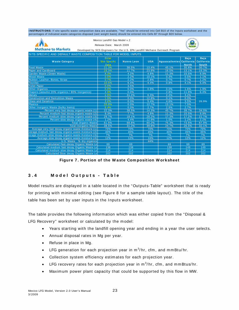